Embed Size (px)
Citation preview

Chapter 5Calculating Functional Programs
Jeremy Gibbons
Abstract. Functional programs are merely equations; they may be ma-nipulated by straightforward equational reasoning. In particular, one canuse this style of reasoning to calculate programs, in the same way thatone calculates numeric values in arithmetic. Many useful theorems forsuch reasoning derive from an algebraic view of programs, built arounddatatypes and their operations. Traditional algebraic methods concen-trate on initial algebras, constructors, and values; dual co-algebraic meth-ods concentrate on final co-algebras, destructors, and processes. Bothmethods are elegant and powerful; they deserve to be combined.
1 Introduction
These lecture notes on algebraic and coalgebraic methods for calculating func-tional programs derive from a series of lectures given at the Summer School onAlgebraic and Coalgebraic Methods in the Mathematics of Program Constructionin Oxford in April 2000. They are based on an earlier series of lectures given atthe Estonian Winter School on Computer Science in Palmse, Estonia, in 1999.
1.1 Why calculate programs?
Over the past few decades there has been a phenomenal growth in the use ofcomputers. Alongside this growth, concern has naturally grown over the cor-rectness of computer systems, for example as regards human safety, financialsecurity, and system development budgets. Problems in developing software anderrors in the final product have serious consequences; such problems are thenorm rather than the exception. There is clearly a need for more reliable meth-ods of program construction than the traditional ad hoc methods in use today.What is needed is a science of programming, instead of today’s craft (or perhapsblack art). As Jeremy Gunawardena points out [15], computation is inherentlymore mathematical than most engineering artifacts; hence, practising softwareengineers should be at least as familiar with the mathematical foundations ofsoftware engineering as other engineers are with the foundations of their ownbranches of engineering.By ‘mathematical foundations’, we do not necessarily mean obscure aspects
of theoretical computer science. Rather, we are referring to simple propertiesand laws of computer programs: equivalences between programming constructs,relationships between well-known algorithms, and so on. In particular, we areinterested in calculating with programs, in the same way that we calculate withnumeric quantities in algebra at school.
5. Calculating Functional Programs 149
1.2 Functional programming
One particularly appropriate framework for program calculation is functionalprogramming, simply because the absence of side-effects ensures referential trans-parency — all that matters of any expression is the value it denotes, not anyother characteristic such as the method by which it computed, the time taken toevaluate it, the number of characters used to express it, and so on. Expressionsin a functional programming language behave as they do in ordinary mathemat-ics, in the sense that an expression in a given context may be replaced with adifferent expression yielding the same value, without changing its meaning inthe surrounding context. This makes calculations much more straightforward.Functional programming is programming with expressions, which denote val-
ues, as opposed to statements, which denote actions. A program consists of acollection of equations defining new functions. For example, here is a simplefunctional program:
square x = x * x
This program defines the function square. The fact that it is written as anequation implies that any occurrence of an expression square x is equivalent tothe expression x * x, whatever the expression x.
1.3 Universal properties
Suppose one has to define a function satisfying a given specification. Two ap-proaches to solving this problem spring to mind. One, the explicit approach, isto provide an implementation of the function. The other, the implicit approach,is to provide a property that completely characterizes the function. Such a prop-erty is known as a universal property. The implicit approach is less direct, andrequires more machinery, but turns out to be more convenient for calculatingwith. Universal properties are a central theme of these lectures.
1.3.1 Example: fork
Given two functions f :: A→ B (which from an A computes a B) and g :: A→ C(which from an A computes a C), consider the problem of constructing a functionof type A→B×C (which from an A computes both a B and a C). We will writethis induced function ‘fork (f , g)’. We will think of fork itself as a higher-orderoperator, taking functions to functions.
1.3.2 Solution using explicit approach
The explicit approach to constructing this function fork consists of providing animplementation
fork (f , g) a = (f a, g a)

150 Jeremy Gibbons
That is, applying the function fork(f , g) to the argument a yields the pair whoseleft component is f a and whose right component is g a. Now the existence ofa solution to the problem is ‘obvious’. (Actually, the existence of solutions toequations like this is a central theme in semantics of functional programming,but that is beyond the scope of these lectures.) However, proofs of properties ofthe function can be rather laborious, as we show below.
1.3.3 Projections eliminate fork
We claim thatexl ◦ fork (f , g) = fexr ◦ fork (f , g) = g
where exl and exr are the pair projections or destructors, yielding the left andright components of a pair respectively. (Here, ◦ is function composition; exl ◦fork (f , g) is the composition of the two functions exl and fork (f , g), so that
(exl ◦ fork (f , g)) a = exl (fork (f , g) a)for any a.) The proof of the first property is as follows:
(exl ◦ fork (f , g)) a=
{composition
}
exl (fork (f , g) a)=
{fork
}
exl (f a, g a)=
{exl
}
f a
and so exl◦fork(f , g) = f as required. The proof of the second property is similar.
1.3.4 Any pair-forming function is a fork
We claim that, for pair-forming h (that is, h :: A→ B× C),fork (exl ◦ h, exr ◦ h) = h
To prove this, assume an arbitrary a, and suppose that h a = (b, c) for someparticular b and c; then
fork (exl ◦ h, exr ◦ h) a=
{fork, composition
}
(exl (h a), exr (h a))=
{h
}
(exl (b, c), exr (b, c))=
{exl, exr
}
(b, c)=
{h
}
h a
as required.

5. Calculating Functional Programs 151
1.3.5 Identity function is a fork
We claim that
fork (exl, exr) = id
The proof:
fork (exl, exr) (a, b)
={fork
}
(exl (a, b), exr (a, b))
={exl, exr
}
(a, b)
={identity
}
id (a, b)
1.3.6 Solution using implicit approach
The implicit approach to constructing the function fork consists of observingthat fork (f , g) is uniquely determined by the fact that it returns the pair withcomponents given by f and g . That is, fork (f , g) is the unique solution of theequations
exl ◦ h = fexr ◦ h = g
in the unknown h. Equivalently, we have the universal property of fork
h = fork (f , g)⇔ exl ◦ h = f ∧ exr ◦ h = g
It is perhaps not immediately obvious that the system of two equations above hasa unique solution (we address this problem later). But, once we can justify theuniversal property, calculations with forks become much more straightforward,as we illustrate below.
1.3.7 Projections eliminate fork
For the claim
exl ◦ fork (f , g) = fexr ◦ fork (f , g) = g
we have the proof
exl ◦ fork (f , g) = f ∧ exr ◦ fork (f , g) = g
⇔ {universal property, letting h = fork (f , g)
}
fork (f , g) = fork (f , g)

152 Jeremy Gibbons
1.3.8 Any pair-forming function is a fork
For the claim that, for pair-forming h,fork (exl ◦ h, exr ◦ h) = h
we have the proofh = fork (exl ◦ h, exr ◦ h)
⇔ {universal property, letting f = exl ◦ h and g = exr ◦ h
}
exl ◦ h = exl ◦ h ∧ exr ◦ h = exr ◦ h
1.3.9 Identity function is a fork
For the claim thatfork (exl, exr) = id
we have the proofid = fork (exl, exr)
⇔ {universal property, letting f = exl and g = exr
}
exl ◦ id = exl ∧ exr ◦ id = exr
The gain is even more impressive for recursive functions, where the explicitapproach requires inductive proofs that the implicit approach avoids. We willsee many examples of such gains throughout these lectures.
1.4 The categorical approach to datatypes
In these lectures we will be using category theory as an organizing principle. Forour purposes, the use of category theory can be summarized in three slogans:
• A model of computation is represented by a category.• Types and programs in the model are represented by the objects and arrowsof that category.
• A type constructor in the model is represented by a functor on that category.We will not rely on any deep results of category theory; we will only be usingthe theory to obtain a streamlined notation.
1.4.1 Definition of a category
A category C consists of a collection Obj(C) of objects and a collection Arr(C) ofarrows, such that
• each arrow f in Arr(C) has a source src(f ) and a target tgt(f ), both objectsin Obj(C) (we write ‘f : src(f )→ tgt(f )’);
• for every object A in Obj(C) there is an identity arrow idA : A→ A;• arrows g : A→ B and f : B→ C compose to form an arrow f ◦ g : A→ C;• composition is associative: f ◦ (g ◦ h) = (f ◦ g) ◦ h;• the appropriate identity arrows are units: for arrow f : A → B, we havef ◦ idA = f = idB ◦ f .

5. Calculating Functional Programs 153
1.4.2 An example category: SetThe category Set of sets and total functions is defined as follows.• The objects Obj(Set) are sets of values, or types.• The arrows f : A→B in Arr(Set) are total functions equipped with domain Aand range B.
• The identity arrows are the identity functions idA a = a.• Composition of arrows is functional composition: (f ◦ g) a = f (g a).
For example, addition is an arrow from the object Int × Int (the set of pairs ofintegers) to the object Int (the set of integers).
1.4.3 Definition of a functor
An (endo)-functor F is an operation on the objects and arrows of a category:
• F A is an object of C when A is an object of C;• F f is an arrow of C when f is an arrow of C.which respects source and target:
F f : F (src(f ))→ F(tgt(f ))
respects composition:
F (f ◦ g) = F f ◦ F g
and respects identities:
F idA = idF A
1.4.4 An example functor in Set : Pair
The Set functor Pair is defined as follows.• On objects, Pair A = {(a1, a2) | a1 ∈ A, a2 ∈ A}.• On arrows, (Pair f ) (a1, a2) = (f a1, f a2).We should check that the properties are satisfied (Exercise 1.7.1):
• source and target: Pair f : Pair A→ Pair B when f : A→ B;• composition: Pair (f ◦ g) = Pair f ◦ Pair g ;• identities: Pair idA = idPair A.
1.4.5 More functors
See Exercise 1.7.2 for the proofs that the following are functors.
Identity functor: The simplest functor Id is defined by
Id A = AId f = f

154 Jeremy Gibbons
Constant functor: The next most simple is the constant functor B for objectB, defined by
B A = BB f = idB
List functor: On an object A, this functor yields List A, the type of finite se-quences of values all of type A; on arrows, Listf : ListA→ListB when f : A→B‘maps’ f over a sequence.
Composition of functors: For functors F and G, functor F ◦ G is defined by
(F ◦ G) A = F (G A)(F ◦ G) f = F (G f )
1.4.6 Binary functors
The notion of a functor may be generalized to functors of more than one argu-ment. A bifunctor F is a binary operation on the objects and arrows of a categorywhich respects source and target:
F (f , g) : F(src(f ), src(g))→ F(tgt(f ), tgt(g))
respects composition:
F (f ◦ g , h ◦ k) = F (f , h) ◦ F (g , k)
and respects identities:
F (idA, idB) = idF(A,B)
1.4.7 Examples of bifunctors
See Exercise 1.7.3 for the proofs that the following are bifunctors.
Product: (a generalization of Pair)
A× B = {(a, b) | a ∈ A, b ∈ B}(f × g) (a, b) = (f a, g b)
Projection functors:
A� B = Af � g = f
1.4.8 Making monofunctors out of bifunctors
Here are two ways of constructing a monofunctor (that is, a functor of a singleargument) from a bifunctor.
Sectioning: for bifunctor ⊕ and object A, functor (A⊕) is defined by(A⊕) B = A⊕ B(A⊕) f = idA ⊕ f
(so (A�) = A, for example), and similarly in the other argument.
5. Calculating Functional Programs 155
Lifting: for bifunctor ⊕ and monofunctors F and G, functor F ⊕G is defined by
(F ⊕ G) A = F A⊕ G A(F ⊕ G) f = F f ⊕ G f
See Exercise 1.7.4 for the proofs that these do indeed define functors.
1.5 The pair calculus
The pair calculus is an elegant theory of operators on pairs. We have already seenthe product bifunctor, one of the two main ingredients of the calculus. The othermain ingredient is the coproduct bifunctor, the dual of the product, obtained by‘turning all the arrows around’ in the definition of product. Along with universalproperties, duality is another central theme of these lectures.
1.5.1 Product bifunctor
As we saw above, product × forms a bifunctor; in Set , for types A and B, thetype A × B consists of pairs (a, b) where a :: A and b :: B. We saw earlier theproduct destructors exl ::A×B→A and exr ::A×B→B. We also saw the productmorphisms (‘forks’) f � g :: A→ B × C when f :: A→ B and g :: A→ C, definedby the universal property
h = f � g ⇔ exl ◦ h = f ∧ exr ◦ h = g
(Some would write ‘〈f , g〉’ where we now write ‘f �g ’.) Now we can define productmap (that is, the action of the product bifunctor on arrows) using fork:
f × g = (f ◦ exl) � (g ◦ exr)
Here are some properties of fork and product:
exl ◦ (f � g) = fexr ◦ (f � g) = g(exl ◦ h) � (exr ◦ h) = hexl � exr = id(f × g) ◦ (h � k) = (f ◦ h) � (g ◦ k)id× id = id(f × g) ◦ (h × k) = (f ◦ h)× (g ◦ k)(f � g) ◦ h = (f ◦ h) � (g ◦ h)
The proofs are simple consequences of the universal property. We have seen someproofs already; see also Exercise 1.7.5.
1.5.2 Coproduct bifunctor
We define the Set bifunctor + on objects byA+ B = {inl a | a ∈ A} ∪ {inr b | b ∈ B}

156 Jeremy Gibbons
The intention here is that inl and inr are injections such that inl a and inr b aredistinct, even when a = b; thus, coproduct gives a disjoint union. (For example,one might define inl and inr by
inl a = (0, a)inr b = (1, b)
but we will not assume any particular definition.) The coproduct constructorsare the functions inl :: A→ A+ B and inr :: B→ A+ B. We define the coproductmorphisms (‘joins’) f � g :: A + B→ C when f :: A→ C and g :: B→ C, by theuniversal property
h = f � g ⇔ h ◦ inl = f ∧ h ◦ inr = g
(Some would write ‘[f , g ]’ where we write ‘f � g ’.) We can now define coproductmap using a join:
f + g = (inl ◦ f ) � (inr ◦ g)
Here are some properties of join and coproduct:
(f � g) ◦ inl = f(f � g) ◦ inr = g(h ◦ inl) � (h ◦ inr) = hinl � inr = id(f � g) ◦ (h + k) = (f ◦ h) � (g ◦ k)id+ id = id(f + g) ◦ (h + k) = (f ◦ h) + (g ◦ k)h ◦ (f � g) = (h ◦ f ) � (h ◦ g)
See Exercise 1.7.5 for the proofs.
1.5.3 Duality
Notice that each of the above properties of join and coproduct is the dual ofa property of fork and product, obtained by reversing the order of compositionand by exchanging products, forks, and destructors for coproducts, joins andconstructors. Duality gives a ‘looking-glass world’, in which everything is themirror image of something in the ‘everyday’ world.
1.5.4 Exchange law
Here is a law relating products and coproducts, a bridge between the everydayworld and the looking-glass world:
(f � g) � (h � j ) = (f � h) � (g � j )
⇔ {universal property of �
}
exl ◦ ((f � g) � (h � j )) = f � h ∧exr ◦ ((f � g) � (h � j )) = g � j

5. Calculating Functional Programs 157
⇔ {composition distributes over join
}
(exl ◦ (f � g)) � (exl ◦ (h � j )) = f � h ∧(exr ◦ (f � g)) � (exr ◦ (h � j )) = g � j
⇔ {projections eliminate forks
}
true
In fact, there is also a dual proof, using the universal property of joins (Exer-cise 1.7.6); one might think of it as a proof from the other side of the looking-glass.
1.5.5 Distributivity
In Set , the objects A × (B + C) and (A × B) + (A × C) are isomorphic. We saythat Set is a distributive category. The isomorphism in one direction,
undistl :: (A× B) + (A× C)→ A× (B+ C)
is easy to write, in two different ways (Exercise 1.7.7):
undistl = (exl � exl) � (exr + exr)= (id× inl) � (id× inr)
We could also have defined it in a pointwise style:
undistl (inl (a, b)) = (a, inl b)undistl (inr (a, c)) = (a, inr c)
The inverse operation
distl :: A× (B+ C)→ (A× B) + (A× C)
is straightforward to define in a pointwise style:
distl (a, inl b) = inl (a, b)distl (a, inr c) = inr (a, c)
Moreover, these two functions are indeed inverses, as is easy to verify.However, this inverse cannot be defined in a pointfree style in terms of the
product and coproduct operations alone. (Indeed, some categories have productsand coproducts, and hence a function undistl as defined above, but no inversefunction distl, and so are not distributive categories. Typically, such categoriesdo not support definitions in a pointwise style. The category Rel of sets andbinary relations is an example.)
1.5.6 Booleans and conditionals
In a distributive category, we can model the datatype of booleans by
Bool = 1+ 1true = inl ()false = inr ()

158 Jeremy Gibbons
where () is the unique element of the unit type 1. For predicate p :: A→ Bool,we define the guard
p? :: A→ (A+ A)p? = (exl+ exl) ◦ distl ◦ (id � p)
or, in an equivalent pointwise form,
p? x = inl x , if p x= inr x , otherwise
We can then define the conditionalif p then f else g = (f � g) ◦ p?
1.6 Bibliographic notes
The program calculation field is a flourishing branch of programming methodol-ogy. One recent textbook (based on a theory of relations rather than functions,but similar in spirit to the material presented in these lectures) is [4]. Also rel-evant are the proceedings of the Mathematics of Program Construction confer-ences [39, 2, 30, 21]. There are many good books on functional programming ; werecommend [5] in particular. The classic reference for category theory is [23], butthis is rather heavy going for non-mathematicians; for a computing perspective,we recommend [8, 9, 31, 45].The observation that universal properties are very convenient for calculating
programs was made originally by Backhouse [1]. The categorical approach todatatypes dates back to the ADJ group [13, 14] in the 1970’s, but was broughtback into fashion by Hagino [16, 17] and Malcolm [24, 25]. The pair calculus isprobably folklore, but our presentation of it was inspired by Malcolm’s thesis.The claim that distributive categories are the appropriate venue for discussingdatatypes is championed mainly by Walters [44–46].
1.7 Exercises
1. Check that Pair (as defined in §1.4.4) does indeed satisfy the propertiesrequired of a functor.
2. Check that operations claimed in §1.4.5 to be functors (identity, constant,list, composition) satisfy the necessary properties.
3. Check that operations claimed in §1.4.7 to be bifunctors (×, �) satisfy thenecessary properties.
4. Check that sectioning and lifting operations claimed in §1.4.8 to constructmonofunctors from bifunctors satisfy the necessary properties.
5. Prove the properties of product (from §1.5.1) and of coproduct (from §1.5.2)using the corresponding universal properties.
6. Prove the exchange law from §1.5.4(f � g) � (h � j ) = (f � h) � (g � j )
using the universal property of joins (instead of the universal property offorks).

5. Calculating Functional Programs 159
7. Prove the equivalence of the two characterizations of undistl from §1.5.5:(exl � exl) � (exr + exr) = (id× inl) � (id× inr)
In fact, there are two different proofs, one for each universal property.8. Prove the following properties of conditionals:
h ◦ if p then f else g = if p then h ◦ f else h ◦ g(if p then f else g) ◦ h = if p ◦ h then f ◦ h else g ◦ hif p then f else f = fif not ◦ p then f else g = if p then g else fif const true then f else g = fif p then (if q then f else g)
else (if q then h else j )= if q then (if p then f else h)
else (if p then g else j )
(Here, not is negation of booleans, and const is the function such thatconst a b = a for any b.)
2 Recursive datatypes in the category Set
The pair calculus is elegant, but not very powerful; descriptive power comes withrecursive datatypes. In this section we will discuss a simple first approximationto what we really want, namely recursive datatypes in the category Set . We willconstruct monomorphic and polymorphic datatypes, and their duals. However,there are inherent limitations in working within the category Set , which we willremedy in Section 3.
2.1 Overview
The Haskell-style recursive datatype definitions
data IntList = Nil | Cons Int IntListdata List a = Nil | Cons a (List a)
(one monomorphic, one polymorphic) give for free:
• a ‘map’ operator;• a ‘fold’ (like join for coproducts), to consume a data structure;• an ‘unfold’ (like fork for products), to generate a data structure;• universal properties for fold and unfold;• a number of theorems about fold and unfold.
Actually, we will discover that we cannot simultaneously achieve all of these goalsin Set , which will motivate the move to another category, Cpo, in Section 3.

160 Jeremy Gibbons
2.2 Monomorphic datatypes
We consider first the case of monomorphic datatypes. The first problem is toidentify a common form, encompassing all the datatype declarations in whichwe are interested. Consider the Haskell-style datatype definition
data IntList = Nil | Cons Int IntList
This defines two constructors
Nil :: IntListCons :: Int→ (IntList→ IntList)
Different datatype definitions, of course, will introduce different constructors.This raises some problems for a general theory:
• there may be arbitrarily many constructors;• the constructors may be constants or functions;• the constructor functions may be of arbitrary arities.
How can we circumvent these problems, and unify all datatype definitions intoa common form?
2.2.1 Unifying constructors
The third problem identified above, constructors of arbitrary arities, can beresolved by ‘uncurrying’ the constructor functions; that is, by tupling the argu-ments together using products. For example, the binary Cons constructor forlists introduced above is equivalent to the unary constructor
Cons :: Int× IntList→ IntList
The second problem, that some constructors may be constants rather than func-tions, can be resolved by treating a constant constructor such as Nil as a functionfrom the unit type 1:
Nil :: 1→ IntList
Now the first problem, of an arbitrary number of constructors, may be resolvedby taking the join of the existing collection of unary constructor functions (be-cause they all share a common target, the defined type):
Nil � Cons :: 1+ (Int× IntList)→ IntList
This yields a single constructor Nil � Cons. Being a constructor for the definedtype IntList, its target type is that type. Its source type 1+(Int× IntList) is sometype expression involving the target type IntList— in fact, some functor appliedto IntList.
5. Calculating Functional Programs 161
2.2.2 Datatype definitions
Therefore, it suffices to consider datatypes T with a single unified constructorinT :: F T→ T for some functor F. We write
T = data F
For example, for IntList, the functor is FIntList, where
FIntList X = 1+ (Int× X)
That is,
FIntList = 1 + (Int × Id)
so we could defineIntList = data (1 + (Int × Id))
2.3 Folds
We have identified a common form for all monomorphic datatype definitions.However, datatypes are not much use without functions over them. It is nowwidely accepted that program structure should, where possible, reflect datastructure [18]. Accordingly, we should identify a program structure that reflectsthe data structure of monomorphic datatypes. It turns out that the right kind ofstructure is one of homomorphisms between algebras, which we explore in thissection.
2.3.1 Fixpoints
The definition ‘T = data F’ defines T to be a fixpoint of the functor F; that is, Tis isomorphic to FT. In one direction, the isomorphism is given by inT ::FT→T.In the other direction, we suppose an inverse outT :: T → F T. (In fact, we seehow to define outT shortly.)However, to say that the datatype definition ‘T = data F’ defines T to be
a fixpoint of the functor F does not completely determine T, as a functor mayhave more than one fixpoint. For example, the types ‘finite sequences of integers’and ‘finite and infinite sequences of integers’ are both fixpoints of the functorFIntList (Exercise 2.9.3). Informally, what we want is the ‘least fixpoint’, thatis, the ‘smallest such type’ — finite rather than finite-and-infinite sequences ofintegers. How can we formalize this idea?
2.3.2 Algebras
We define an F-algebra to be a pair (A, f ) such that f :: F A → A. Thus, thedatatype definition T = data F defines (T, inT) to be an F-algebra. For example,(IntList,Nil � Cons) is an FIntList-algebra. However, F-algebras are not uniqueeither. For example, (Int, zero � plus) is another FIntList-algebra (Exercise 2.9.4),where zero ::1→Int and plus ::Int×Int→Int; that is, zero�plus ::1+(Int×Int)→Int.

162 Jeremy Gibbons
2.3.3 Homomorphisms
A homomorphism between F-algebras (A, f ) and (B, g) is a function h :: A→ Bsuch that
h ◦ f = g ◦ F h
Pictorially,
F Af ✲ A
F B
F h
❄
g✲ B
h
❄
For example, the function sum :: IntList→ Int, which sums an IntList,
sum (Nil ()) = 0sum (Cons (a, x )) = a + sum x
is a homomorphism from (IntList,Nil � Cons) to (Int, zero � plus), because
sum ◦ (Nil � Cons) = (zero � plus) ◦ FIntList sum
(see Exercise 2.9.5).
2.3.4 Initial algebras
We say that an F-algebra (A, f ) is initial if, for any F-algebra (B, g), there isa unique homomorphism from (A, f ) to (B, g). Then the datatype definition‘T = data F’ defines (T, inT) to be ‘the’ initial F-algebra. There may be morethan one initial algebra, but all initial algebras are equivalent (Exercise 2.9.6);thus, it does not really matter which one we pick.
2.3.5 Existence of initial algebras
It is well-known that for polynomial F (built out of identity and constant functorsusing product and coproduct) on many categories including Set and Rel , initialalgebras always exist. Malcolm [24] shows existence also for regular F (addingfixpoints), allowing us to define mutually recursive datatypes such as
data IntTree = Node Int IntForestdata IntForest = Empty | ConsF IntTree IntForest
2.3.6 Definition of folds
Suppose that (T, inT) is the initial F-algebra. Then there is a unique homomor-phism to any F-algebra (B, f ) — that is, for any such f , there exists a uniqueh such that h ◦ inT = f ◦ F h. We would like a notation for ‘the unique solution

5. Calculating Functional Programs 163
h of this equation involving f ’; we write ‘foldT f ’ for this unique solution. Thus,foldT f has type T→ B when f :: F B→ B. Pictorially,
F Tin ✲ T
F B
F (foldT f )
❄
f✲ B
foldT f
❄
Uniqueness provides the universal property
h = foldT f ⇔ h ◦ inT = f ◦ F h
2.4 Polymorphic datatypes
The type IntList has the ‘base type’ Int built in: it cannot be used for listsof booleans, lists of strings, and so on. We would like polymorphic datatypes,parameterized by an arbitrary base type A: lists of As, trees of As, and so on.For example, the Haskell-style type definition
data List a = Nil | Cons a (List a)
defines a type List A for each type A; now List is a type constructor, whereasIntList is just a type.
2.4.1 Using bifunctors
The essential idea in constructing polymorphic datatypes is to use a bifunctor ⊕.A polymorphic type T is then defined by sectioning ⊕ with the type parameteras one argument, and then taking the fixpoint:
T A = data (A⊕)Now the constructor has type
inT A :: A⊕ T A→ T A
though usually we will write just ‘inT’ as a polymorphic function, omitting theA. For example, we can define a polymorphic list type by
List A = data (A⊕)where
A⊕ B = 1+ (A× B)
Equivalently, we could write
List A = data (1 + (A × Id))
without naming the bifunctor.

164 Jeremy Gibbons
2.4.2 Polymorphic folds
Folds over monomorphic datatypes generalize in a straightforward fashion topolymorphic datatypes. The datatype definition
T A = data (A⊕)defines (T A, inT) to be the initial (A⊕)-algebra; therefore there exists a uniquehomomorphism foldT A f to any other (A⊕)-algebra (B, f ). (Again, we will usuallywrite just ‘foldT f ’, leaving the fold operator polymorphic in A.) The fold foldT fhas type T A→ B when f :: A⊕ B→ B; pictorially,
A⊕ T AinT ✲ T A
A⊕ B
id⊕ foldT f
❄
f✲ B
foldT f
❄
Uniqueness gives the universal propertyh = foldT f ⇔ h ◦ inT = f ◦ (id⊕ h)
2.4.3 Making it a functor: map
The datatype definition T A = data (A⊕) makes T a type constructor, anoperation on types. This suggests that perhaps we can make T a functor: all weneed is a corresponding operation on functions T f with type T A→ T B whenf ::A→B (satisfying the functor laws). We define T f = foldT A (inT B ◦ (f ⊕ id)).Pictorially,
A⊕ T AinT A ✲ T A
A⊕ T B
id⊕ T f
❄
f ⊕ id✲ B⊕ T B
inT B
✲ T B
T f
❄
(We should check that this does indeed satisfy the requirements for being afunctor; see Exercise 2.9.7.) For historical reasons, we will write ‘mapT f ’ ratherthan ‘T f ’.
2.5 Properties of folds
There are a number of general theorems about folds that arise as simple con-sequences of the universal property. These include: an evaluation rule, whichshows ‘one step of evaluation’ of a fold; an exact fusion law, which states whena function can be fused with a fold; a weak fusion law, a simpler but weakercorollary of the exact fusion law; the identity law, which states that the identityfunction is a fold; and a definition of the destructor of a datatype as a fold.

5. Calculating Functional Programs 165
2.5.1 Evaluation rule
The evaluation rule describes the composition of a fold and the constructors ofits type; informally, it gives ‘one step of evaluation’ of the fold.
foldT f ◦ inT
={universal property, letting h = fold f
}
f ◦ F (foldT f )
2.5.2 Fusion (exact version)
Fusion laws for folds are of the form
h ◦ foldT f = foldT g ⇔ . . .
(or sometimes with the composition the other way around). They give condi-tions under which one can fuse two computations, one a fold, to yield a singlemonolithic computation. In this case, we have
h ◦ foldT f = foldT g
⇔ {universal property
}
h ◦ foldT f ◦ inT = g ◦ F (h ◦ foldT f )
⇔ {functors
}
h ◦ foldT f ◦ inT = g ◦ F h ◦ F (foldT f )
⇔ {evaluation rule
}
h ◦ f ◦ F (foldT f ) = g ◦ F h ◦ F (foldT f )
2.5.3 Fusion (weaker version)
The above fusion law is an equivalence, so it is as strong as possible. However, itis a little unwieldy, because the premise (the last line in the calculation above)is rather long. Here is a fusion law with a simpler but stronger premise (whichtherefore is a weaker law).
h ◦ foldT f = foldT g
⇔ {exact fusion
}
h ◦ f ◦ F (foldT f ) = g ◦ F h ◦ F (foldT f )
⇐ {Leibniz
}
h ◦ f = g ◦ F h

166 Jeremy Gibbons
2.5.4 Identity
The identity function id is a fold:
id = foldT f⇔ {
universal property}
id ◦ inT = f ◦ F id
⇔ {identity
}
f = inT
That is, foldT inT = id.
2.5.5 Destructors
Also, the destructor outT of a datatype, the inverse of the constructor inT, canbe written as a fold; this is known as Lambek’s Lemma.
inT ◦ foldT f = id
⇔ {identity as a fold
}
inT ◦ foldT f = foldT inT
⇐ {weak fusion
}
inT ◦ f = inT ◦ F inT
⇐ {Leibniz
}
f = F inT
Therefore we can defineoutT = foldT (F inT)
We should check that this also makes out the inverse of in when the compositionis reversed:
outT ◦ inT
={above
}
foldT (F inT) ◦ inT
={evaluation rule
}
F inT ◦ F outT=
{functors
}
F (inT ◦ outT)=
{in ◦ out = id
}
id
Lambek’s Lemma is a corollary of the more general theorem that an injectivefunction (that is, a function with a post-inverse) on a recursive datatype is afold (Exercise 2.9.8). Since the destructor is by assumption the inverse of theconstructors, it is injective.

5. Calculating Functional Programs 167
2.6 Co-datatypes and unfolds
All of this theory of datatypes dualizes, to give a theory of co-datatypes andunfolds. The dualization is quite straightforward; nevertheless, we present thefacts here for completeness.
2.6.1 Co-algebras and homomorphisms
An F-co-algebra is a pair (A, f ) such that f ::A→FA. A homomorphism betweenF-co-algebras (A, f ) and (B, g) is a function h :: A→ B such that
F h ◦ f = g ◦ h
Pictorially,
Af ✲ F A
B
h
❄
g✲ F B
F h
❄
An F-co-algebra (A, f ) is final if, for any F-co-algebra (B, g), there is a uniquehomomorphism from (B, g) to (A, f ). The datatype definition T = codata Fdefines (T, outT) to be ‘the’ final F-co-algebra.
2.6.2 Unfolds
Suppose that (T, outT) is the final F-co-algebra. Then there is a unique homomor-phism to (T, outT) from any F-co-algebra (B, f ) — that is, there exists a uniqueh such that outT ◦ h = F h ◦ f . We write ‘unfoldT f ’ for this homomorphism. Theunfold unfoldT f has type B→ T when f :: B→ F B:
Bf ✲ F B
T
unfoldT f
❄
outT✲ F T
F (unfoldT f )
❄
Uniqueness provides the universal property
h = unfoldT f ⇔ outT ◦ h = F h ◦ f

168 Jeremy Gibbons
2.6.3 Polymorphic co-datatypes
In the same way,
T A = codata (A⊕)defines a polymorphic co-datatype, with destructor
outT A :: T A→ A⊕ T A
This induces a polymorphic unfold with universal property
h = unfoldT A f ⇔ outT ◦ h = (id⊕h) ◦ fThe typing is unfoldT f :: B→ T A when f :: B→ A⊕ B; pictorially,
Bf ✲ A⊕ B
T A
unfoldT f
❄
outT✲ A⊕ T A
id⊕ unfoldT f
❄
Co-datatypes too form functors; the map for f :: A→ B is given by
mapT A f = unfoldT B ((f⊕id) ◦ outT A)
2.6.4 An example: streams
The polymorphic datatype of streams (infinite lists) is defined
Stream A = codata (A×)Thus, the destructor for this type is outStream :: Stream A→ A × Stream A. Theunfold unfoldStream f has type A→ Stream B for f :: A→ B× A. For example,
from = unfoldStream Int (id � (1+))
yields increasing streams of naturals: from n = n,n + 1,n + 2, . . .. For anotherexample,
fibs = (unfoldStream Int (exl � (exr � plus))) (0, 1)
defines the Fibonacci sequence 0, 1, 1, 2, 3, 5, 8, . . ..
2.6.5 Properties of unfolds
The theorems dualize too, of course. See Exercise 2.9.10 for the proofs.
Evaluation rule:
outT ◦ unfoldT f = F (unfoldT f ) ◦ f

5. Calculating Functional Programs 169
Exact and weak fusion:unfoldT f ◦ h = unfoldT g
⇔ F (unfoldT f ) ◦ f ◦ h = F (unfoldT f ) ◦ F h ◦ g⇐ f ◦ h = F h ◦ g
Identity:
unfoldT outT = id
Constructors: (the dual of the ‘destructor’ law for folds)
inT = unfoldT (F outT)
Again, this dual is a corollary of a more general law (Exercise 2.9.11), thatany surjective function (one with a pre-inverse) to a recursive datatype is anunfold.
2.6.6 Example: insertion sort
Given the datatype List A = data (1 + (A × Id)), suppose we have an insertionoperation
ins :: 1+ (A× List A)→ List A
that gives an empty list, or inserts an element into a sorted list. Then insertionsort is defined by
insertsort = foldList ins
2.6.7 Example: selection sort
Given the codatatype CList A = codata (1 + (A × Id)), suppose we have anoperation
del :: CList A→ 1+ (A× CList A)
that finds and removes the minimum element of a non-empty list. Then selectionsort is defined by
selectsort = unfoldCList del
2.7 . . . and never the twain shall meet
Unfortunately, this elegant theory is severely limited when it comes to actualprogramming. Datatypes and co-datatypes are different things, so one cannotcombine them. For example, one cannot write programs of the form ‘unfold thenfold’; one instance of this scheme is quicksort, which builds a binary search tree(an unfold) then flattens it to a list (a fold), and another is mergesort, which re-peatedly halves a list (unfolding to a tree) then repeatedly merges the fragments(folding the tree). This pattern of computation is known as a hylomorphism, andis very common in programming.

170 Jeremy Gibbons
Moreover, Set is not a good model of programs. As it contains only totalfunctions, it necessarily suffers from some lack of power, and corresponds onlyvaguely to most programming languages. (Indeed, the selection sort given in§2.6.7 does not really work: the function del is necessarily partial, as it makesno sense on an infinite list, and so neither del nor selectsort are arrows in Set .)The solution to both problems is to move to the category Cpo, imposing more
structure on the objects and arrows of the category than there is in Set .
2.8 Bibliographic notes
As mentioned in the bibliographic notes for the previous section, the categori-cal approach to datatypes is due originally to the ADJ group [13, 14] and laterto Hagino [16, 17]. However, the presentation in these notes owes more to Mal-colm [24, 25]. The proof that, for the kinds of functor that interest us, initialalgebras and final coalgebras always exist, is (a corollary of a more generaltheorem) due to Smyth and Plotkin [34]. The term ‘hylomorphism’ is due toMeijer [27].
2.9 Exercises
1. Translate the following Haskell-style definition of binary trees with booleanexternal labels into the categorical style:
data BoolTree = Tip Bool | Bin BoolTree BoolTree
2. Translate the following categorical-style datatype definition
StringTree = data (1 + (Id × String × Id))
into your favourite programming languages (for example, Haskell, Modula 2,Java).
3. Show that the types ‘finite sequences of integers’ and ‘finite and infinitesequences of integers’ are both fixpoints of the functor 1 + (Int × Id).
4. Check that (IntList,Nil � Cons) and (Int, zero � plus) are FIntList-algebras,where
zero () = 0plus (m,n) = m + n
5. Check that sum, the function which sums an IntList,
sum (Nil ()) = 0sum (Cons (a, x )) = a + sum x
is an FIntList-homomorphism from (IntList,Nil � Cons) to (Int, zero � plus).6. Show that any two initial F-algebras are isomorphic. (Hint: the identity func-tion is a homomorphism from an F-algebra to itself; use uniqueness.) So,given the existence of an initial algebra, we are justified in talking about‘the’ initial algebra.

5. Calculating Functional Programs 171
7. Check that defining
T f = foldT A (inT B ◦ (f ⊕ id))
does indeed make T a functor.8. Show that if g ◦ h = idT for recursive datatype T, then h is a fold. Thus, anyinjective function on a recursive datatype is a fold.
9. In fact, one can say something stronger. Show that h is a fold for recursivedatatype data F if and only if ker (F h) ⊆ ker (h ◦ in), where the kernelker f of a function f ::A→B is the set of pairs { (a, a ′) ∈ A×A | f a = f a ′ }.Use this to solve Exercise 2.9.8.
10. Prove the properties of unfolds from §2.6.5, using the universal property.11. Dually to Exercise 2.9.8, show that any surjective function to a recursivedatatype is an unfold.
12. Dually to Exercise 2.9.9, show that h is a unfold for recursive codatatypecodata F if and only if img (F h) ⊇ img (out ◦ h), where the image img f ofa function f :: A→ B is the set { b ∈ B | ∃a ∈ A. f a = b }. Use this to solveExercise 2.9.11.
13. Prove that the fork of two folds is a fold:foldT f � foldT g = foldT ((f ◦ F exl) � (g ◦ F exr))
(This is known fondly as the ‘banana split theorem’, by those who know thefork operation as ‘split’ and write folds using ‘banana brackets’.)
14. Prove the special cases fold-map fusion
foldT f ◦ mapT g = foldT (f ◦ (g ⊕ id))
of the fusion law for folds, and map-unfold fusion
mapT g ◦ unfoldT f = unfoldT ((g ⊕ id) ◦ f )
of the fusion law for unfolds.15. For datatype T = data F, Meertens [26] defines the notion of a paramor-
phism paraT f :: T→ C when f :: F (C× T)→ C as follows:
paraT f = exl ◦ foldT (f � (inT ◦ F exr))
It enjoys the universal property
h = paraT f ⇔ h ◦ inT = f ◦ F (h � id)
Informally, a paramorphism is a generalization of a fold: the result on a largerstructure may depend on results on substructures, but also on the substruc-tures themselves. For example, the factorial function is a paramorphism overthe naturals:
fact = paraNat (const 1 � (mult ◦ (id× succ)))where constab = a and mult multiplies a pair of numbers. That is, fact0 = 1,and fact (succ n) = mult (fact n, succ n).(a) Show that the second component of the above fold is merely the identityfunction:exr ◦ foldT (f � (inT ◦ F exr)) = id
Hence foldT (f � (inT ◦ F exr)) = paraT f � id.

172 Jeremy Gibbons
(b) Show that the identity function is a paramorphism:
id = para (in ◦ F exl)
(c) Prove the (weak) fusion law for paramorphisms:
h ◦ para f = para g ⇐ h ◦ f = g ◦ F (h × id)
(d) Show that any fold is a paramorphism:
fold f = para (f ◦ F exl)
(This is a generalization of Exercise 2.9.15b.)(e) Show that any function on a recursive datatype can be written as aparamorphism:
h = para (h ◦ in ◦ F exr)
Thus, paramorphisms are extremely general.16. On the codatatype of lists from §2.6.7, define as an unfold the function
interval , such that
interval (1, 5) = [1, 2, 3, 4, 5]interval (5, 5) = [5]interval (6, 5) = [ ]
17. On the codatatype StreamA = codata (A×), the function iterate is definedby
iterate f = unfoldStream (id � f )
Using unfold fusion, prove that
map f ◦ iterate f = iterate f ◦ f
18. For codatatype T = codata F, Uustalu and Vene [40, 38] dualize paramor-phisms to get apomorphisms apoT f :: C → T when f :: C → F (C + T) asfollows:
apoT f = unfoldT (f � (F inr ◦ outT)) ◦ inl
They enjoy the universal property
h = apoT f ⇔ outT ◦ h = F (h � id) ◦ f
Informally, an apomorphism is a generalization of an unfold: a larger struc-ture may be generated recursively from new seeds, but may also be generated‘all at once’ without recursion. For example, on the codatatype CList A =codata (1 + (A × Id)) of lists, the append function is an apomorphism:
append = apoClist f
wheref (x , y) = inl (), if null x ∧ null y
= inr (head y , inr (tail y)), if null x ∧ not (null y)= inr (head x , inl (tail x , y)), if not (null x )
That is, append(x , y) is the empty list if both are empty, cons (head y , tail y)(which is just y) if only x is empty, and cons (head x , append (tail x , y)) if

5. Calculating Functional Programs 173
neither x nor y is empty. This definition copies just the first list; in contrast,the simple unfold characterization of append
append = unfoldCList g
whereg (x , y) = inl (), if null x ∧ null y
= inr (head y , (x , tail y)), if null x ∧ not (null y),= inr (head x , (tail x , y)), if not (null x )
copies both lists.(a) Show that on the second summand the above unfold acts merely as theidentity function:
unfoldT (f � (F inr ◦ outT)) ◦ inr = id
Hence unfoldT (f � (F inr ◦ outT)) = apoT f � id.(b) Show that the identity function is an apomorphism:
id = apo (F inl ◦ out)
(c) Prove the (weak) fusion law for apomorphisms:
apo f ◦ h = apo g ⇐ f ◦ h = F (h + id) ◦ g
(d) Show that any unfold is an apomorphism:
unfold f = apo (F inl ◦ f )
(This is a generalization of Exercise 2.9.18b.)(e) Show that any function yielding a recursive datatype can be written asan apomorphism:
h = apo (F inr ◦ out ◦ h)
(f) Write ins ::A×CListA→CListA, which inserts a value into a sorted list,as an apomorphism.
19. Datatypes and codatatypes for the same functor are different structures, butthey are not unrelated. Suppose we have the datatype definitions
T = data FU = codata F
Lambek’s Lemma shows how to write outT ::T→ F T, giving an F-coalgebra(T, outT) and hence a function unfoldU outT ::T→U. This function ‘coerces’an element of T to the type U. Give the dual construction, expressing thiscoercion as a fold. Prove (in two different ways) that these two coercions areequal. Thus, we have two ways of writing the coercion from the datatypeT to the codatatype U, and no way of going back again. This is what onemight expect: embedding finite lists into finite-or-infinite lists is easy, butthe opposite embedding is more difficult. In the following section we moveto a setting in which the two types coincide, and so the coercions becomethe identity function.

174 Jeremy Gibbons
3 Recursive datatypes in the category CpoAs we observed above, the simple and elegant model of datatypes and the cor-responding characterization of the ‘natural patterns’ of recursion over them inthe category Set has a number of problems. We solve these problems by movingto the category Cpo. This category is a refinement of the category Set . Somestructure is imposed on the objects of the category, so that they are no longermerely sets of unrelated elements, and correspondingly some structure is inducedon the arrows. Some things become neater (for example, we will be able to com-pose unfolds and folds) but some things become messier (specifically, strictnessconditions have to be attached to some of the laws).
3.1 The category Cpo
The category Cpo has as objects pointed complete partial orders: sets equippedwith a partial order on the elements, with a least element and closed under limitsof ascending chains. The arrows are continuous functions on these structuredsets: functions which distribute over limits of ascending chains. (We will explainthese notions below.)Intuitively, we will use the partial order to represent ‘approximations’ in a
‘definedness’ or ‘information’ ordering: x � y will mean that element x is anapproximation to (or less well defined than, or provides less information than)element y . Closure under limits means that we can consider complex, perhapsinfinite, structures as the limit of their finite approximations, and be assured thatsuch limits always exist. Continuity means that computations (that is, arrows)respect these limits: the behaviour of a computation on the limit of a chain ofapproximations can be understood purely in terms of its behaviour on each ofthe approximations.
3.1.1 Posets
A poset is a pair (A,�), where A is a set and � is a partial order on A. That is,the following properties hold of �:
reflexivity: a � atransitivity: a � b and b � c imply a � cantisymmetry: a � b and b � a imply a = b
The least element of a poset (A,�) is the a ∈ A such that a � a ′ for alla ′ ∈ A, if this element exists. By antisymmetry, a poset has at most one leastelement. The upper bounds in A of the poset (B,�) where B ⊆ A are the elements{a ∈ A | b � a for all b ∈ B}; note that they are elements of A, and notnecessarily of B. The least upper bound (lub)
⊔B in A of the poset (B,�) where
B ⊆ A is the least element of the upper bounds in A of (B,�), if this leastelement exists.

5. Calculating Functional Programs 175
3.1.2 Cpos and pcpos
A chain 〈ai〉 in a poset (A,�) is a sequence a0, a1, a2 . . . of elements in A suchthat a0 � a1 � a2 � · · ·. The lub of the chain 〈ai〉, if it exists, is denoted
⊔i〈ai〉.
A poset (A,�) is a complete partial order (cpo) if every chain of elements in Ahas a lub in A. A cpo is a pointed cpo (pcpo) if it has a least element (which isdenoted ⊥A). From now on, we will often write just ‘A’ instead of ‘(A,�)’ for apcpo.
3.1.3 Strictness, monotonicity and continuity
A function f :: A→ B between pcpos A and B is strict if
f ⊥A = ⊥B
A function f :: A→ B between pcpos (A,�A) and (B,�B) is monotonic if
a �A a ′ ⇒ f a �B f a ′
A monotonic function between pcpos A and B is continuous if
f (⊔
i〈ai〉) =⊔
i(〈f ai〉)
3.1.4 Examples of pcpos
The following are all pcpos:
• for set A such that ⊥ �∈ A, the lifted discrete set {⊥} ∪ A with ordering
a � b ⇔ a = ⊥ ∨ a = b
• for pcpos A and B, the cartesian product {(a, b) | a ∈ A ∧ b ∈ B} withordering
(a, b) � (a ′, b′)⇔ a �A a ′ ∧ b �B b′
(so the least element is (⊥A,⊥B));• for pcpos A and B, the separated sum {⊥}∪{(0, a) | a ∈ A}∪{(1, b) | b ∈ B}with ordering
x � y ⇔ (x = ⊥) ∨(x = (0, a) ∧ y = (0, a ′) ∧ a �A a ′) ∨(x = (1, b) ∧ y = (1, b′) ∧ b �B b′)
• for pcpos A and B, the set of continuous functions from A to B, with ordering
f � g ⇔ (f a �B g a for all a ∈ A)
(so the least element is the function f such that f a = ⊥B for any a).

176 Jeremy Gibbons
3.1.5 Modelling datatypes in CpoAs suggested above, the idea is that we will use pcpos to model datatypes. Theelements of a pcpo model (possibly partially defined) values of that type. Theordering � models ‘is no more defined than’ or ‘approximates’. For example,(⊥,⊥) � (1,⊥) � (1, 2) and (⊥,⊥) � (⊥, 2) � (1, 2), but (1,⊥) and (⊥, 2)are unrelated. ‘Completely defined’ values are the lubs of chains of approxima-tions. All ‘reasonable’ functions are continuous, so we are justified in restrictingattention just to continuous functions.
3.1.6 The category
We move from the category Set to the category Cpo. The objects Obj(Cpo) arepcpos; the arrows Arr(Cpo) are continuous functions between pcpos. Later, wewill also use the category Cpo⊥, which has the same objects, but only the strictcontinuous functions as arrows.
3.2 Continuous algebras
Fokkinga and Meijer [11] have generalized the Set-based definitions of datatypesand their morphisms to Cpo. This provides a number of advantages over Set :• we can now model partial functions, because all types have a least-definedelement that can be used as the ‘meaning’ of an undefined computation;
• unfolds generate and folds consume the same kind of entity, so they can becomposed to form hylomorphisms;
• we can give a meaning to arbitrary recursive definitions, not just to foldsand unfolds.
(However, these advantages come at the cost of a more complex theory.) In theselectures we will only use the middle benefit of the three.
3.2.1 The main theorem
A functor F is locally continuous if, for all objects A and B, the action of F onfunctions of type A → B is continuous. All functors that we will be using arelocally continuous.Suppose F is a locally continuous functor on Cpo. Suppose also that F pre-
serves strictness, that is, F f is strict when f is strict; so F is also a functoron Cpo⊥. Then there exists an object T, and strict functions inT :: F T→ T andoutT ::T→ F T, each the inverse of the other; hence T is isomorphic to F T. Thefunctor F determines T up to isomorphism, and T uniquely determines inT andoutT. We write
T = fix F
The pair (T, inT) is the initial F-algebra in Cpo⊥; that is, for any type A andstrict function f :: F A→ A, there is a unique strict h satisfying the equation

5. Calculating Functional Programs 177
h ◦ inT = f ◦ F h
We write foldT f for this unique solution. It has the universal property that
h = foldT f ⇔ h ◦ inT = f ◦ F h for strict f and h
(The strictness condition on f is necessary; see Exercise 3.6.1.)Also, the pair (T, outT) is the final F-co-algebra in Cpo; that is, for any type
A and (not necessarily strict) function f ::A→FA, there is a unique h satisfying
outT ◦ h = F h ◦ f
We write unfoldTf for this unique solution. It has the universal property (withoutany strictness conditions)
h = unfoldT f ⇔ outT ◦ h = F h ◦ f
(Apparently the strictness requirements of folds and unfolds are asymmetric.Exercise 3.6.2 shows that this apparent asymmetry is illusory.)
3.3 The pair calculus again
The cool, clear waters of the pair calculus are muddied slightly by the presenceof ⊥ and the possibility of non-strict functions. The cartesian product worksfine, as before; all the same properties hold. Unfortunately, the separated sum isno longer a proper coproduct, because the injections inl and inr are non-strict,and so the equations
h ◦ inl = f ∧ h ◦ inr = g
no longer have a unique solution (because they do not specify h ⊥). However,there is a unique strict solution, which is the one we take for join:
h = f � g ⇔ h ◦ inl = f ∧ h ◦ inr = g ∧ h strict
Such strictness conditions are the price we pay for the extra power and flexibilityof Cpo. In view of this, we use the term ‘sum’ instead of ‘coproduct’ from nowon.
3.3.1 Distributivity
Even worse than the extra strictness conditions, we no longer have a distributivecategory: product no longer distributes over sum. Because the function distl takes(a,⊥) to ⊥, there is no way of inverting it to retrieve the a. There is moreinformation in A× (B+C) than in (A×B) + (A×C); now distl ◦ undistl = id butundistl ◦ distl � id. Nevertheless, we continue to use the guard p?, but with care:for example, the equation
if p then f else f = f
now holds only for total p (more precisely, when p x = ⊥ implies f x = ⊥).

178 Jeremy Gibbons
3.4 Hylomorphisms
So much for the disadvantages. To compensate, we can now express the commonpattern of computation of an unfold followed by a fold, because now unfoldsproduce and folds consume the same kind of datatype. We present two exampleshere: quicksort and mergesort.
3.4.1 Lists
We use the datatype
List A = fix (1 + (A × Id))
of possibly-empty lists. For brevity, we define separate constructors
nil = in (inl ())cons (a, x ) = in (inr (a, x ))
and destructors
isNil = (const true � const false) ◦ outhead = (⊥ � exl) ◦ outtail = (⊥ � exr) ◦ out
We introduce the following syntactic sugar for folds on this type:
foldL :: (B× (A× B→ B))→ List A→ BfoldL (e, f ) = foldList (const e � f )
unfoldL :: ((B→ Bool)× (B→ A× B))→ B→ List AunfoldL (p, f ) = unfoldList ((const () + f ) ◦ p?)
For example, concatenation on these lists is given by
cat (x , y) = foldL (y , cons) x
3.4.2 Flatten
We also use the datatype
Tree A = fix (1 + (A × (Id × Id)))
of internally-labelled binary trees, for which the fold may be sweetened to
foldT :: (B× (A× (B× B)→ B))→ Tree A→ BfoldT (e, f ) = foldTree (const e � f )
The function flatten turns one of these trees into a possibly-empty list:
flatten :: Tree A→ List Aflatten = foldT (nil , glue)glue (a, (x , y)) = cat (x , cons (a, y))
5. Calculating Functional Programs 179
3.4.3 Partition
The function filter takes a predicate p and a list x , and returns a pair of lists:those elements of x that satisfy p, and those elements of x that do not.
filter :: (A→ Bool)→ List A→ List A× List Afilter p = foldL ((nil ,nil), step)step (a, (x , y)) = (cons (a, x ), y), if p a
= (x , cons (a, y)), otherwise
An alternative, point-free but perhaps less clear, definition of step is
step = if p then (cons ◦ (id× exl)) � (exr ◦ exr)else (exl ◦ exr) � (cons ◦ (id× exr))
For example, we can partition a non-empty list into those elements of the tailthat are less than the head, and those elements of the tail that are not:
partition :: List A→ List A× List Apartition x = filter (< head x ) (tail x )
3.4.4 Quicksort
The unfold on our type of trees is equivalent to
unfoldT :: ((B→ Bool)× (B→ A)× (B→ B× B))→ B→ Tree AunfoldT (p, f , g) = unfoldTree ((const () + (f � g)) ◦ p?)
Now we can build a binary search tree from a list:
buildBST :: List A→ Tree AbuildBST = unfoldT (isNil , head , partition)
(Note that partition is applied only to non-empty lists.) Then we can sort bybuilding then flattening a tree:
quicksort :: List A→ List Aquicksort = flatten ◦ buildBST
This is a fold after an unfold.
3.4.5 Merge
For this example, we define the datatype
PList A = fix (A + (A × Id))
of non-empty lists. Again, for brevity, we define separate destructors
isSing = (const true � const false) ◦ outhd = (id � exl) ◦ outtl = (⊥ � exr) ◦ out
We also specialize the unfold to
unfoldPL :: ((B→ Bool)×(B→ A)×(B→ B))→ B→ PList A

180 Jeremy Gibbons
unfoldPL (p, f , g) = unfoldPList ((f + (f � g)) ◦ p?)
Then the function merge, which merges a pair of sorted lists into a single sortedlist, is
merge :: PList A× PList A→ PList Amerge = unfoldPL (p, f , g) ◦ inl
wherep = const false � isSingf = (min ◦ (hd × hd)) � hdg (inl (x , y)) = inr y , if hd x ≤ hd y ∧ isSing x
= inl (tl x , y), if hd x ≤ hd y ∧ not (isSing x )= inr x , if hd x > hd y ∧ isSing y= inl (x , tl y), if hd x > hd y ∧ not (isSing y)
g (inr x ) = inr (tl x )
and min is the binary minimum operator. Note that the ‘state’ for the unfold iseither a pair of lists (which are to be merged) or a single list (which is simply tobe copied). Exercise 3.6.9 concerns the characterization of merge as an apomor-phism, whereby the single list is copied to the result ‘all in one go’ rather thanelement by element.
3.4.6 Split
Similarly, we define separate constructors
wrap a = in (inl a)cons (a, x ) = in (inr (a, x ))
and specialize the fold to
foldPL :: ((A→ B)× (A× B→ B))→ PList A→ BfoldPL (f , g) = foldPList (f � g)
Then non-singleton lists can be split into two roughly equal halves:
split :: PList A→ PList A× PList Asplit x = foldPL (step, start (hd x )) (tl x ) where
start a b = (wrap a,wrap b)step (a, (y , z )) = (cons (a, z ), y)
3.4.7 Mergesort
We also define the datatype
PTree A = fix (A + (Id × Id))
of non-empty externally-labelled binary trees. We use the specializations
foldPT :: ((A→ B)× (B× B→ B))→ PTree A→ BfoldPT (f , g) = foldPTree (f � g)
of fold, and

5. Calculating Functional Programs 181
unfoldPT :: ((B→ Bool)× (B→ A)× (B→ B× B))→ B→ PList AunfoldPT (p, f , g) = unfoldPTree ((f + g) ◦ p?)
of unfold. Then mergesort is
foldPT (wrap,merge) ◦ unfoldPT (isSing , hd , split)
(Note that split is applied only to non-singleton lists.)
3.5 Bibliographic notes
Complete partial orders are standard material from denotational semantics; seefor example [10] for a straightforward algebraic point of view, and [33, 35] forthe specifics of the applications to denotational semantics. Meijer, Fokkinga andPaterson [27] argue for the move from Set to Cpo. The Main Theorem above isfrom [11], where it is in turn acknowledged to be another corollary of the resultsof Smyth and Plotkin [34] and Reynolds [32] mentioned earlier.
3.6 Exercises
1. Show that, even for strict f , the equation
h ◦ inT = f ◦ F h
may have non-strict solutions for h as well as the unique strict solution.Thus, the strictness condition on the universal property of fold in §3.2.1 isnecessary.
2. Show that the categorical dual of the notion of ‘strictness’ vacuously holds ofany function. Therefore there really is no asymmetry between the universalproperties of fold and unfold in §3.2.1.
3. Show that the definitions of map as a fold (§2.4.3) and as an unfold (§2.6.3)are equal in Cpo.
4. Suppose T = fix F. Let functor G be defined by G X = F (X × T), and letU = fix G. Show that any paramorphism (Exercise 2.9.15) on T can bewritten as a hylomorphism, in the form of a fold (on U) after predsT, where
predsT = unfoldU (F (id � id) ◦ outT)
5. The datatype of natural numbers is Nat = fix (1+). (Actually, this typenecessarily includes also ‘partial numbers’ and one ‘infinite number’ as wellas all the finite ones.) We can define the following syntactic sugar for thefolds and unfolds:
foldN :: (A× (A→ A))→ Nat→ AfoldN (e, f ) = foldNat (const e � f )
unfoldN :: ((A→ Bool)× (A→ A))→ A→ NatunfoldN (p, f ) = unfoldNat ((const () + f ) ◦ p?)
Informally, foldN (e, f )n computes f n e, by n-fold application of f to e, andunfoldN (p, f )x returns the least n such that f n x satisfies p. Write addition,

182 Jeremy Gibbons
subtraction, multiplication, division, exponentiation and logarithms on nat-urals, using folds and unfolds as the only form of recursion. (Hint: define a‘predecessor’ function using the destructor outNat, but make it total, takingzero to zero. You may find it easier to make division and logarithms roundup rather than down.)
6. Using the datatype of lists from §3.4.1, write the insertion functionins :: 1+ (A× List A)→ List A
as an unfold. Hence write insertsort using folds and unfolds as the only formof recursion.
7. Using the same datatype as in Exercise 3.6.6, write the deletion function
del :: List A→ 1+ (A× List A)
as a fold. Hence write selectsort using folds and unfolds as the only form ofrecursion.
8. Eratosthenes’ Sieve is a method for generating primes. It maintains a col-lection of ‘candidates’ as a stream, initially containing [2, 3, . . .]. The firstelement of the collection is a prime; a new collection is obtained by deletingall multiples of that prime. Write this program using folds and unfolds onstreams as the only form of recursion. (You can use mod on natural num-bers.)
9. Write merge from §3.4.5 as an apomorphism rather than an unfold.10. Show that if
h = foldT g ◦ unfoldT f
thenh = g ◦ F h ◦ f
(Indeed, this is an equivalence, not just an implication; but the proof in theopposite direction requires some machinery that we have not covered.) Thisis a fusion law for hylomorphisms, sometimes known as deforestation: insteadof separate unfold and fold phases, the two can be combined into a singlemonolithic recursion, which does not explicitly construct the intermediatedata structure. The now absent datatype T is sometimes known as a virtualdata structure [36].
11. On Stream A = fix (A×), define as an unfold a functiondo :: (A→ A)→ A→ Stream A
such that dosa returns the infinite stream a, sa, s (sa) and so on. Also defineas a fold a function while :: (A→ Bool)→ Stream A→ A such that while p xyields the first element of stream x that satisfies p. Now while p ◦do s modelsa while loop in an imperative language. Use deforestation (Exercise 3.6.10)to calculate a function whiledo such that whiledo (p, s) = while p ◦ do s, butwhich does not generate the intermediate stream.
12. Write the function whiledo from Exercise 3.6.11 using the folds and unfoldson naturals (Exercise 3.6.5) instead of on streams. (Hint: whiledo (p, s) xapplies s a certain number n of times; the number n is the least such thatsn x fails to satisfy p.)

5. Calculating Functional Programs 183
13. Folds and unfolds on the datatype of streams are sufficient to compute arbi-trary fixpoints, so give the complete power of recursive programming. Thefixpoint-finding function fix is defined using explicit recursion by
fix :: (A→ A)→ Afix f = f (fix f )
Equivalently, given the function apply :: (A→B)×A→B, it may be defined
fix f = apply (f ,fix f )
Show that fix may also be defined as the composition of a stream fold (usingapply) and a stream unfold (generating infinitely many copies of a value).Use deforestation (Exercise 3.6.10) to remove the intermediate stream, andshow that this yields the explicitly recursive characterization of fix . (Thisexercise is due to Graham Hutton [20].)
14. Under certain circumstances, the post-inverse of a fold is an unfold, and thepre-inverse of an unfold is a fold:
unfoldT f ◦ foldT g = id ⇐ f ◦ g = id
Prove this law.15. The function cross takes two infinite streams of values, and returns an infinitestream containing every possible pair of values, the first component drawnfrom the first list and the second component drawn from the second list.The difficulty is in enumerating this two-dimensional collection in a suitableorder; the standard approach is diagonalization. Define
cross = concat ◦ diagonals
where
diagonals :: Stream A× Stream B→ Stream (List (A× B))concat :: Stream (List (A× B))→ Stream (A× B)
Express cross as a hylomorphism (that is, express diagonals as an unfold,and concat as a fold). (Hint: first construct the obvious stream of streamsincorporating all possible pairs. Then the ‘state’ of the iteration for diagonalsconsists of a pair, a finite list of those streams seen so far and a streamof streams not yet seen. At each step, strip another diagonal off from thestreams seen so far, and include another stream from those not yet seen.)This example is due to Richard Bird [3].
4 Applications
We conclude these lecture notes with three more substantial examples of theconcepts we have described: a simple compiler for arithmetic expressions; lawsfor monads and comonads; and efficient programs for breadth-first traversal oftrees.

184 Jeremy Gibbons
4.1 A simple compiler
In this example, we define a datatype of simple (arithmetic) expressions. Wepresent the obvious recursive algorithm for evaluating such expressions; it turnsout to be a fold. We also develop a compiler to translate such expressions intocode for a stack machine; this too turns out to be a fold. Clearly, running thecompiled code should be equivalent to evaluating the original expression. Theproof of this fact turns out to be a straightforward application of the universalproperties concerned.
4.1.1 Expressions and evaluation
We assume a datatype Op of operators. The arities of the operators are givenby a function arity ::Op→Nat. We also assume a datatype Val of values, and afunction apply ::Op×ListVal→Val (where List is as in §3.4.1) to characterize theoperators. Operator application is partial: apply (op, args) is defined only whenarity op = length args, where length computes the length of a list. Now we candefine a datatype of expressions
Expr = fix (Op × List)
on which evaluation, which provides the ‘denotational semantics’ of an expres-sion, is simply a fold:
eval = foldExpr apply :: Expr→ Val
4.1.2 Compilation
For the ‘operational semantics’, we assume a datatype Instr of instructions, andan encoding code :: Op→ Instr of operators as instructions. Then compilation isalso a fold:
compile :: Expr→ List Instrcompile = fold (cons ◦ (code × concat))
Here, concat :: List (List A)→ List A, and cons :: A× List A→ List A.
4.1.3 An example
For example, we might want to manipulate expressions like
2✍✌✎�
3✍✌✎�
4✍✌✎�
5✍✌✎�
+✍✌✎�
+✍✌✎�
×✍✌✎�
We could define in Haskell

5. Calculating Functional Programs 185
> data Op = Sum | Product | Num Int> type Val = Int
> arity Sum = 2> arity Product = 2> arity (Num x) = 0
> apply (Sum, [x,y]) = x+y> apply (Product, [x,y]) = x*y> apply (Num x, []) = x
> data Instr = Bop ((Val,Val)->Val) | Push Val
> code Sum = Bop (uncurry (+))> code Product = Bop (uncurry (*))> code (Num x) = Push x
and so the compiled code of the example expression will be
[Bop mul, Bop add, Push 2, Push 3, Bop add, Push 4, Push 5]where add = uncurry (+)
mul = uncurry (*)
4.1.4 Execution steps
We assume also a single-step execution function
exec :: Instr→ List Val→ List Val
such thatexec (code op) (cat args vals) = cons (apply (op, args), vals)
when arity op = length args. Continuing the example, we might have
> exec (Bop f) (x:y:xs) = f (x,y) : xs> exec (Push x) xs = x : xs
4.1.5 Complete execution
Now, running the program may be defined as follows:
run :: List Instr→ List Val→ List Valrun nil vals = valsrun (cons (instr , prog)) vals = exec instr (run prog vals)
Equivalently, discarding the last variable:

186 Jeremy Gibbons
run nil = idrun (cons (instr , prog)) = exec instr ◦ run prog
Define comp (f , g) = f ◦ g , and its curried version comp′ f g = comp (f , g); then
run = foldL′ (id, comp′ ◦ exec)
(where foldL′ :: (B× (A→B→B))→ List A→B, using a curried function as oneof its arguments). Equivalently again
run = compose ◦ map exec
where
compose :: List (A→ A)→ (A→ A)compose = foldL′ (id, comp′)
4.1.6 The correctness criterion
We assume that expressions are well-formed, each operator having exactly theright number of arguments. Then compiling an expression and running the re-sulting code on a given starting stack should have the effect of prefixing thevalue of that expression onto the stack:
run (compile expr) vals = cons (eval expr , vals)
Equivalently, discarding the last two variables,
run ◦ compile = cons ′ ◦ eval
where cons ′ is the curried version of cons.
4.1.7 Strategy
The universal property of fold on expressions is
h = fold f⇔h ◦ in = f ◦ (id×map h)
We will use this universal property to show that both operational semanticsrun ◦ compile and denotational semantics cons ′ ◦ eval above are folds. We wantto find an f such that
run ◦ compile ◦ in = f ◦ (id×map (run ◦ compile))
so that run ◦ compile = fold f . Then to complete the proof, we need only showthat, for the same f ,
cons ′ ◦ eval ◦ in = f ◦ (id×map (cons ′ ◦ eval))

5. Calculating Functional Programs 187
4.1.8 Operational semantics as a fold
Now,run ◦ compile ◦ in
={compile = fold (cons ◦ (code × concat))}
run ◦ cons ◦ (code × concat) ◦ (id×map compile)=
{run ◦ cons = comp ◦ (exec × run)}
comp ◦ (exec × run) ◦ (code × concat) ◦ (id×map compile)=
{pairs
}
comp ◦ ((exec ◦ code)× (run ◦ concat ◦ map compile))=
{run ◦ concat = compose ◦ map run
}
comp ◦ ((exec ◦ code)× (compose ◦ map run ◦ map compile))
and sorun ◦ compile = fold (comp ◦ ((exec ◦ code)× compose))
4.1.9 Denotational semantics as a fold
We have(cons ′ ◦ eval ◦ in) (op, exprs)
={eval = fold apply
}
cons ′ (apply (op,map eval exprs))=
{arity op = length exprs; requirement of exec
}
exec (code op) ◦ cat (map eval exprs)=
{cat = compose ◦ map cons ′
}
exec (code op) ◦ compose (map (cons ′ ◦ eval) exprs)=
{pairs
}
(comp ◦ ((exec ◦ code)× (compose ◦ map (cons ′ ◦ eval)))) (op, exprs)
and socons ′ ◦ eval = fold (comp ◦ ((exec ◦ code)× compose))
too, completing the proof.
4.2 Monads and comonads
Monads and comonads are categorical concepts; each consists of a type functorand a couple of operations that satisfy certain laws. They turn out to haveuseful applications in the semantics of programming languages. A monad canbe used to model a notion of computation; in a sense, monads correspond tooperational semantics. Dually, comonads correspond to denotational semanticsof programming languages. But we will not get into that here. Rather, we simplyobserve that many constructions in functional programming are either monadsor comonads, and that the proofs of the monad and comonad laws are oftensimple applications of the universal properties of the functors concerned. Wepresent two simple examples, one a monad and the other a comonad.

188 Jeremy Gibbons
4.2.1 Monads
A monad is a functor M together with two operationsunit :: A→MAmult :: M (MA)→MA
The two operations should be natural transformations, which is to say that thelaws
unit ◦ f = M f ◦ unitmult ◦ M (M f ) = M f ◦ mult
should be satisfied. Moreover, the following ‘coherence laws’ relating the twooperations should hold:
mult ◦ unit = idmult ◦ M unit = idmult ◦ mult = mult ◦ Mmult
4.2.2 The list monad
Ordinary lists are one example of a monad. The datatype is defined in §3.4.1.We define the two functions
wrap a = cons (a,nil)concat = foldL (nil , cat)
We claim that List is a monad, with unit wrap and multiplication concat .
4.2.3 Laws
We must verify the following five laws:wrap ◦ f = map f ◦ wrapconcat ◦ map (map f ) = map f ◦ concatconcat ◦ wrap = idconcat ◦ map wrap = idconcat ◦ concat = concat ◦ map concat
We address them one by one.
4.2.4 Naturality of unit
(map f ◦ wrap) a=
{wrap
}
map f (cons (a,nil))=
{map
}
cons (f a,nil)=
{wrap
}
(wrap ◦ f ) a

5. Calculating Functional Programs 189
4.2.5 Naturality of mult
map f ◦ concat
={concat
}
map f ◦ foldL (nil , cat)
={fusion: map f ◦ cat = cat ◦ (map f ×map f )
}
foldL (nil , cat ◦ (map f × id))
={fold-map fusion (Exercise 2.9.14)
}
foldL (nil , cat) ◦ map (map f )
={concat
}
concat ◦ map (map f )
4.2.6 Mult-unit
(concat ◦ wrap) x
={wrap
}
concat (cons (x ,nil))
={concat
}
x
={identity
}
id x
4.2.7 Mult-map-unit
concat ◦ map wrap
={fold-map fusion
}
foldL (nil , cat ◦ (wrap × id))
={cat ◦ (wrap × id) = cons
}
foldL (nil , cons)
={identity as a fold
}
id

190 Jeremy Gibbons
4.2.8 Mult-mult
concat ◦ concat
={concat
}
concat ◦ foldL (nil , cat)
={fold fusion: concat ◦ cat = cat ◦ (concat × concat)}
foldL (nil , cat ◦ (concat × id))
={fold-map fusion
}
concat ◦ map concat
4.2.9 Comonads
Dually, a comonad is a functor M together with two operations
extr :: MA→ Adupl :: MA→M (MA)
Again, the two operations should be natural transformations:
f ◦ extr = extr ◦ M fM (M f ) ◦ dupl = dupl ◦ M f
Moreover, the following coherence laws should hold:
extr ◦ dupl = idM extr ◦ dupl = iddupl ◦ dupl = M dupl ◦ dupl
4.2.10 The stream comonad
One example of a comonad is the datatype of streams:
Stream A = fix (A×)We introduce the separate destructors
head = exl ◦ outtail = exr ◦ out
Thus, the function tails, which turns a stream into the stream of streams of allof its infinite suffices, is an unfold:
tails = unfoldStream (id � tail)
We claim that Stream is a comonad, with extraction head and duplication tails.
5. Calculating Functional Programs 191
4.2.11 Laws
To say that the datatype of streams is a comonad with the above operations isto claim the following five laws:
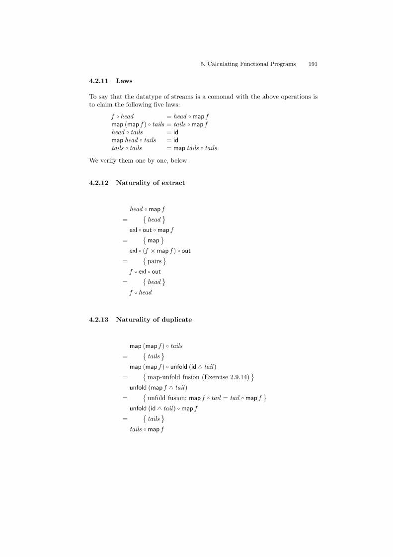
f ◦ head = head ◦ map fmap (map f ) ◦ tails = tails ◦ map fhead ◦ tails = idmap head ◦ tails = idtails ◦ tails = map tails ◦ tails
We verify them one by one, below.
4.2.12 Naturality of extract
head ◦ map f
={head
}
exl ◦ out ◦ map f
={map
}
exl ◦ (f ×map f ) ◦ out
={pairs
}
f ◦ exl ◦ out
={head
}
f ◦ head
4.2.13 Naturality of duplicate
map (map f ) ◦ tails
={tails
}
map (map f ) ◦ unfold (id � tail)
={map-unfold fusion (Exercise 2.9.14)
}
unfold (map f � tail)
={unfold fusion: map f ◦ tail = tail ◦ map f
}
unfold (id � tail) ◦ map f
={tails
}
tails ◦ map f

192 Jeremy Gibbons
4.2.14 Extract-duplicate
head ◦ tails=
{head , tails
}
exl ◦ out ◦ unfold (id � tail)=
{unfolds
}
exl ◦ (id× tails) ◦ (id � tail)=
{pairs
}
id
4.2.15 Map-extract-duplicate
map head ◦ tails=
{tails
}
map head ◦ unfold (id � tail)=
{map-unfold fusion
}
unfold (head � tail)=
{identity as unfold
}
id
4.2.16 Duplicate-duplicate
tails ◦ tails=
{tails
}
unfold (id � tail) ◦ tails=
{unfold fusion: tail ◦ tails = tails ◦ tail
}
unfold (tails � tail)=
{map-unfold fusion
}
map tails ◦ unfold (id � tail)=
{tails
}
map tails ◦ tails
4.3 Breadth-first traversal
As a final example, we discuss breadth-first traversal of a tree. Depth-first traver-sal is an obvious program to write recursively, but breadth-first traversal takesa little more thought; one might say that it ‘goes against the grain’. We presenta number of algorithms, and demonstrate their equivalence.

5. Calculating Functional Programs 193
4.3.1 Lists
Once again, we use the datatype of lists from §3.4.1. We will use the functionconcat , which concatenates a list of lists:
concat = foldL (nil , cat)
4.3.2 Trees
Of course, we will also require a datatype of trees:Tree A = fix (A × List)
for which we introduce the separate destructorsroot = exl ◦ outkids = exr ◦ out
Now, depth-first traversal is easy to write:df = fold (cons ◦ (id× concat))
but breadth-first traversal is a little more difficult.
4.3.3 Levels
The most profitable approach to solving the problem is to split the task into twostages. The first stage computes the levels of tree — a list of lists, organized bylevel:
levels :: Tree A→ List (List A)The second stage is to concatenate the levels. Thus,
bf = concat ◦ levels
4.3.4 Long zip
The crucial component for constructing the levels of a tree is a function lzw (for‘long zip with’), which glues together two lists using a given binary operator:
lzw :: (A× A→ A)→ List A× List A→ List A
Corresponding elements are combined using the binary operator; the remainingelements are merely ‘copied’ to the result. The length of the result is the greaterof the lengths of the arguments. We have
lzw op = unfoldL (p, f )where
p (x , y) = isNil x ∧ isNil yf (x , y) = (head x , (tail x , y)), if isNil y
= (head y , (x , tail y)), if isNil x= (op (head x , head y), (tail x , tail y)), otherwise
(This definition is rather inefficient, as the ‘remaining elements’ are copied one byone. It would be better to use an apomorphism, which would allow the remainderto be copied all in one go; see Exercise 4.5.8.)

194 Jeremy Gibbons
4.3.5 Levels as a fold
Now we can define level-order traversal by
levels = fold (cons ◦ (wrap × glue))where wrapa = cons (a,nil). Here, the function glue glues together the traversalsof the children:
glue = foldL (nil , lzw cat)
4.3.6 Levels as a fold, efficiently
The characterization of levels above is inefficient, because the traversals of chil-dren are re-traversed in building the traversal of the parent. We can use anaccumulating parameter to avoid this problem. We define
levels ′ (t , xss) = lzw cat (levels t , xss)
and so levels t = levels ′ (t ,nil). We can now calculate (Exercise 4.5.9) that
levels ′ (in (a, ts), xss) = cons (cons (a, ys), foldL (yss, levels ′) ts)where (ys, yss) = split xss
wheresplit xss = (nil ,nil), if isNil xss
= (head xss, tail xss), otherwise
With the efficient apomorphic definition of lzw from Exercise 4.5.8, taking timeproportional to the length of the shorter argument, this program for level-ordertraversal takes linear time. However, it is no longer written as a fold.
4.3.7 Levels as an unfold
A better solution is to use an unfold. We generalize to the level-order traversalof a forest :
levelsf :: List (Tree A)→ List (List A)
Again, we can calculate (using the universal property) that levelsf is an unfold:
unfoldL (isNil ,map root � (concat ◦ map kids))
See Exercise 4.5.11 for the details.
4.4 Bibliographic notes
The compiler example was inspired by Hutton [19]. The application of mon-ads to semantics is due to Moggi [28], and of comonads to Brookes [6, 7] andTuri [37]; Wadler [43, 41, 42] brought monads to the attention of functional pro-grammers. The programs for breadth-first tree traversal are joint work withGeraint Jones [12].

5. Calculating Functional Programs 195
4.5 Exercises
1. An alternative definition of compilation is as an unfold, from a list of ex-pressions to a list of instructions. Define compile in this way, and repeat theproof of correctness of the compiler.
2. Use fold-map fusion (Exercise 2.9.14) on lists to show that
foldL′ (id, comp′ ◦ exec) = foldL′ (id, comp) ◦ map exec
(so the two definitions of run in §4.1.5 are indeed equivalent).3. Show that
foldL′ (id, f ) ◦ concat = foldL′ (id, f ) ◦ map (foldL′ (id, f ))
when f is associative. (Hence run ◦ concat = compose ◦ map run).4. The compiler example would be more realistic and more general if the codefor each operation were a list of instructions instead of a single instruction.Repeat the proof for this scenario.
5. The datatype of externally-labelled binary trees from §3.4.7 forms a monad,with unit operation
leaf = in ◦ inl
and multiplication operation
collapse = fold (id � (in ◦ inr))
Prove that the monad laws are satisfied.6. The datatype TreeA = fix (A + (A × (Id × Id))) of homogeneous binary treesforms a comonad, with extraction operation
root = (id � exl) ◦ out
and duplication operation
subs = unfold ((leaf + (node � exr)) ◦ out)
where leaf and node are the separate constructors:
leaf = in ◦ inlnode = in ◦ inr
Prove that the comonad laws are satisfied.7. On the datatype of lists in §3.4.1 we defined concatenation of two lists as afold
cat (x , y) = fold (const y � (in ◦ inr)) x
Calculate a definition as an unfold, using the universal property. Also calcu-late a definition as an apomorphism.
8. Calculate a definition of lzw f (§4.3.4) as an apomorphism.9. Calculate the accumulating-parameter optimization of level-order traversal,from §4.3.6.
10. The program in Exercise 4.5.9 is not a fold. However, if we define insteadthe curried version levels ′′ t xss = levels ′ (t , xss), then levels ′′ is a fold. Usethe universal property to calculate the f such that levels ′′ = fold f .
11. Calculate the version of level-order traversal from §4.3.7 as an unfold.

196 Jeremy Gibbons
12. The final program for breadth-first traversal of a forest was of the form
bff = concat ◦ levelsf
where concat is a list fold and levelsf a list unfold. Use hylomorphism de-forestation (Exercise 3.6.10) to write this as a single recursion, avoiding theintermediate generation of the list of lists. (This program was shown to usby Bernhard Moller [29]; it is interesting that it arises as a ‘mere compileroptimization’ from the more abstract program developed here.)
13. To most people, breadth-first traversal is related to queues, but there are noqueues in the programs presented here. Show that in fact
bff = unfoldL (null , step)
where null holds precisely of empty forests, and step is defined by
step (cons (t , ts)) = (root t , cat (ts, kids ts))
(Hint: the crucial observation is that, for associative operator ⊕ with unite, the equation
foldL (e,⊕) (lzw (⊕) (cons (x , xs), ys))= x ⊕ foldL (e,⊕) (lzw (⊕) (ys, xs))
holds.)
5 Bibliography
1. Roland Backhouse. An exploration of the Bird-Meertens formalism. In Inter-national Summer School on Constructive Algorithmics, Hollum, Ameland. STOPproject, 1989. Also available as Technical Report CS 8810, Department of Com-puter Science, Groningen University, 1988.
2. R. S. Bird, C. C. Morgan, and J. C. P. Woodcock, editors. LNCS 669: Mathematicsof Program Construction. Springer-Verlag, 1993.
3. Richard Bird. Personal communication, 1999.4. Richard Bird and Oege de Moor. The Algebra of Programming. Prentice-Hall,1996.
5. Richard S. Bird. Introduction to Functional Programming Using Haskell. Prentice-Hall, 1998.
6. Stephen Brookes and Shai Geva. Computational comonads and intensional seman-tics. In M. P. Fourman, P. T. Johnstone, and A. M. Pitts, editors, Categories inComputer Science, London Mathematical Society Lecture Notes, pages 1–44. Cam-bridge University Press, 1992. Also Technical Report CMU-CS-91-190, School ofComputer Science, Carnegie Mellon University.
7. Stephen Brookes and Kathryn Van Stone. Monads and comonads in intensionalsemantics. Technical Report CMU-CS-93-140, CMU, 1993.
8. Rod Burstall and David Rydeheard. Computational Category Theory. Prentice-Hall, 1988.
9. Roy L. Crole. Categories for Types. Cambridge University Press, 1994.10. B. A. Davey and H. A. Priestley. Introduction to Lattices and Order. Mathematical
Textbooks Series. Cambridge University Press, 1990.11. Maarten M. Fokkinga and Erik Meijer. Program calculation properties of contin-
uous algebras. Technical Report CS-R9104, CWI, Amsterdam, January 1991.

5. Calculating Functional Programs 197
12. Jeremy Gibbons and Geraint Jones. The under-appreciated unfold. In Proceedingsof the Third ACM SIGPLAN International Conference on Functional Program-ming, pages 273–279, Baltimore, Maryland, September 1998.
13. J. A. Goguen, J. W. Thatcher, E. G. Wagner, and J. B. Wright. An introductionto categories, algebraic theories and algebras. Technical report, IBM Thomas J.Watson Research Centre, Yorktown Heights, April 1975.
14. J. A. Goguen, J. W. Thatcher, E. G. Wagner, and J. B. Wright. Initial algebrasemantics and continuous algebras. Journal of the ACM, 24(1):68–95, January1977.
15. Jeremy Gunawardena. Towards an applied mathematics for computer science. InM. S. Alber, B. Hu, and J. J. Rosenthal, editors, Current and Future Directions inApplied Mathematics. Birkhauser, Boston, 1997.
16. Tatsuya Hagino. A Categorical Programming Language. PhD thesis, Departmentof Computer Science, University of Edinburgh, September 1987.
17. Tatsuya Hagino. A typed lambda calculus with categorical type constructors. InD. H. Pitt, A. Poigne, and D. E. Rydeheard, editors, LNCS 283: Category Theoryand Computer Science, pages 140–157. Springer-Verlag, September 1987.
18. C. A. R. Hoare. Notes on data structuring. In Ole-Johan Dahl, Edsger W. Dijk-stra, and C. A. R. Hoare, editors, Structured Programming, APIC studies in dataprocessing, pages 83–174. Academic Press, 1972.
19. Graham Hutton. Fold and unfold for program semantics. In Proceedings of theThird ACM SIGPLAN International Conference on Functional Programming, Bal-timore, Maryland, September 1998.
20. Graham Hutton. Personal communication, 1999.21. Johan Jeuring, editor. LNCS 1422: Proceedings of Mathematics of Program Con-
struction, Marstrand, Sweden, June 1998. Springer-Verlag.22. Johan Jeuring and Erik Meijer, editors. LNCS 925: Advanced Functional Program-
ming. Springer-Verlag, 1995. Lecture notes from the First International SpringSchool on Advanced Functional Programming Techniques, Bastad, Sweden.
23. Saunders Mac Lane. Categories for the Working Mathematician. Springer-Verlag,1971.
24. Grant Malcolm. Algebraic Data Types and Program Transformation. PhD thesis,Rijksuniversiteit Groningen, September 1990.
25. Grant Malcolm. Data structures and program transformation. Science of ComputerProgramming, 14:255–279, 1990.
26. Lambert Meertens. Paramorphisms. Formal Aspects of Computing, 4(5):413–424,1992.
27. Erik Meijer, Maarten Fokkinga, and Ross Paterson. Functional programming withbananas, lenses, envelopes and barbed wire. In John Hughes, editor, LNCS 523:Functional Programming Languages and Computer Architecture, pages 124–144.Springer-Verlag, 1991.
28. Eugenio Moggi. Notions of computation and monads. Information and Computa-tion, 93(1), 1991.
29. Bernhard Moller. Personal communication, 1995.30. Bernhard Moller, editor. LNCS 947: Mathematics of Program Construction.
Springer-Verlag, 1995.31. Benjamin C. Pierce. Basic Category Theory for Computer Scientists. MIT Press,
1991.32. John C. Reynolds. Semantics of the domain of flow diagrams. Journal of the ACM,
24(3):484–503, 1977.

198 Jeremy Gibbons
33. David A. Schmidt. Denotational Semantics: A Methodology for Language Devel-opment. Allyn and Bacon, 1986.
34. M. B. Smyth and G. D. Plotkin. The category-theoretic solution of recursivedomain equations. SIAM Journal on Computing, 11(4):761–783, November 1982.
35. Joseph Stoy. Denotational Semantics: The Scott-Strachey Approach to Program-ming Language Theory. MIT Press, 1977.
36. Doaitse Swierstra and Oege de Moor. Virtual data structures. In Bernhard Moller,Helmut Partsch, and Steve Schumann, editors, LNCS 755: IFIP TC2/WG2.1State-of-the-Art Report on Formal Program Development, pages 355–371. Springer-Verlag, 1993.
37. Daniele Turi. Functorial Operational Semantics and its Denotational Dual. PhDthesis, Vrije Universiteit Amsterdam, June 1996.
38. Tarmo Uustalu and Varmo Vene. Primitive (co)recursion and course-of-value(co)iteration. Research Report TRITA-IT R 98:02, Dept of Teleinformatics, RoyalInstitute of Technology, Stockholm, January 1998.
39. J. L. A. van de Snepscheut, editor. LNCS 375: Mathematics of Program Construc-tion. Springer-Verlag, 1989.
40. Varmo Vene and Tarmo Uustalu. Functional programming with apomorphisms(corecursion). Proceedings of the Estonian Academy of Sciences: Physics, Mathe-matics, 47(3):147–161, 1998. 9th Nordic Workshop on Programming Theory.
41. Philip Wadler. Comprehending monads. Mathematical Structures in ComputerScience, 2(4):461–493, 1992. Earlier version appeared in ACM Conference on Lispand Functional Programming, 1990.
42. Philip Wadler. The essence of functional programming. In 19th Annual Symposiumon Principles of Programming Languages, 1992.
43. Philip Wadler. Monads for functional programming. In M. Broy, editor, ProgramDesign Calculi: Proceedings of the Marktoberdorf Summer School, 1992. Also in[22].
44. R. F. C. Walters. Datatypes in distributive categories. Bulletin of the AustralianMathematical Society, 40:79–82, 1989.
45. R. F. C. Walters. Categories and Computer Science. Computer Science TextsSeries. Cambridge University Press, 1991.
46. R. F. C. Walters. An imperative language based on distributive categories. Math-ematical Structures in Computer Science, 2:249–256, 1992.
6 Appendix: Implementation in Haskell
The programs we derive in these lectures are easily translated into a lazy func-tional programming language such as Haskell. We present one example, thequicksort program from §3.4, to illustrate.
6.1 Products
We start by encoding the pair calculus. Here are products:
> data Prod a b = Prod a b> exl (Prod a b) = a

5. Calculating Functional Programs 199
> exr (Prod a b) = b
> fork :: (a -> b) -> (a -> c) -> a -> Prod b c> fork f g a = Prod (f a) (g a)
> prod :: (a->c) -> (b->d) -> (Prod a b) -> (Prod c d)> prod f g = fork (f . exl) (g . exr)
6.2 Sums
Here are the definitions for sums:
> data Sum a b = Inl a | Inr b
> join :: (a -> c) -> (b -> c) -> Sum a b -> c> join l r (Inl x) = l x> join l r (Inr y) = r y
> dsum :: (a->c) -> (b->d) -> Sum a b -> Sum c d> dsum f g = join (Inl . f) (Inr . g)
> query :: (a -> Bool) -> a -> Sum a a> query p a | p a = Inl a> | otherwise = Inr a
We include a function query p to model p? (we cannot use the names sum orguard, because they are already used in the standard Haskell prelude).
6.3 Functors
Haskell’s type classes allow us to encode the property of being a functor. Thisallows us to use the same name mapf for the ‘map’ operation of any type functor.(The standard prelude defines the class Functor and the function fmap for thispurpose; we simply repeat the definition with different names here.)
> class TypeFunctor f where> mapf :: (a -> b) -> (f a -> f b)
Actually, all we can encode is the type of the corresponding map operations; wecannot express the laws that should hold.

200 Jeremy Gibbons
6.4 Datatypes
A type functor f induces a datatype Fix f; the constructor is In and the de-structor out. (The difference in capitalization is an artifact of Haskell’s rules foridentifiers.)
> data TypeFunctor f => Fix f = In (f (Fix f))
> out :: TypeFunctor f => Fix f -> f (Fix f)> out (In x) = x
6.5 Folds and unfolds
These are now straightforward translations:
> fold :: TypeFunctor f => (f a -> a) -> (Fix f -> a)> fold f = f . mapf (fold f) . out
> unfold :: TypeFunctor f => (a -> f a) -> (a -> Fix f)> unfold f = In . mapf (unfold f) . f
6.6 Lists
The encoding of a datatype is almost straightforward. The only wrinkle is thatHaskell requires a type constructor identifier (ListF below) in order to makesomething an instance of a type class, so we need to introduce a function toremove this constructor too:
> data ListF a b = ListF (Sum () (Prod a b))> unListF (ListF x) = x
> instance TypeFunctor (ListF a)> where> mapf f (ListF x) = ListF (dsum id (prod id f) x)
Now the datatype itself can be given as a mere synonym:
> type List a = Fix (ListF a)
We introduce some syntactic sugar for functions on lists:
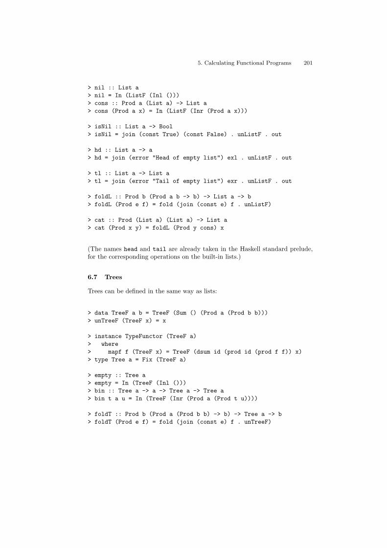
5. Calculating Functional Programs 201
> nil :: List a> nil = In (ListF (Inl ()))> cons :: Prod a (List a) -> List a> cons (Prod a x) = In (ListF (Inr (Prod a x)))
> isNil :: List a -> Bool> isNil = join (const True) (const False) . unListF . out
> hd :: List a -> a> hd = join (error "Head of empty list") exl . unListF . out
> tl :: List a -> List a> tl = join (error "Tail of empty list") exr . unListF . out
> foldL :: Prod b (Prod a b -> b) -> List a -> b> foldL (Prod e f) = fold (join (const e) f . unListF)
> cat :: Prod (List a) (List a) -> List a> cat (Prod x y) = foldL (Prod y cons) x
(The names head and tail are already taken in the Haskell standard prelude,for the corresponding operations on the built-in lists.)
6.7 Trees
Trees can be defined in the same way as lists:
> data TreeF a b = TreeF (Sum () (Prod a (Prod b b)))> unTreeF (TreeF x) = x
> instance TypeFunctor (TreeF a)> where> mapf f (TreeF x) = TreeF (dsum id (prod id (prod f f)) x)> type Tree a = Fix (TreeF a)
> empty :: Tree a> empty = In (TreeF (Inl ()))> bin :: Tree a -> a -> Tree a -> Tree a> bin t a u = In (TreeF (Inr (Prod a (Prod t u))))
> foldT :: Prod b (Prod a (Prod b b) -> b) -> Tree a -> b> foldT (Prod e f) = fold (join (const e) f . unTreeF)

202 Jeremy Gibbons
> unfoldT :: Prod (b -> Bool) (Prod (b -> a) (b -> Prod b b))> -> b -> Tree a> unfoldT (Prod p (Prod f g))> = unfold (TreeF . dsum (const ()) (fork f g) . query p)
6.8 Quicksort
The flattening stage of Quicksort encodes simply:
> flatten :: Tree a -> List a> flatten = foldT (Prod nil glue)> where glue (Prod a (Prod x y)) = cat (Prod x (cons (Prod a y)))
We define filtering as follows (the name filter is already taken):
> filt :: (a -> Bool) -> List a -> Prod (List a) (List a)> filt p = foldL (Prod (Prod nil nil) step)> where step = join (fork (cons . prod id exl) (exr . exr))> (fork (exl . exr) (cons . prod id exr))> . query (p . exl)
The definition of step here is a point-free presentation of the more perspicuousdefinition using variable names and pattern guards:
where step (Prod a (Prod x y))| p a = Prod (cons (Prod a x)) y| otherwise = Prod x (cons (Prod a y))
Now partitioning a non-empty list is an application of filter:
> partition :: Ord a => List a -> Prod (List a) (List a)> partition x = filt (< hd x) (tl x)
(The context ‘Ord a =>’ states that this definition is only applicable to orderedtypes, namely those supporting the operation <.)Then the remainder of the Quicksort algorithm translates naturally:
> build :: Ord a => List a -> Tree a> build = unfoldT (Prod isNil (Prod hd partition))

5. Calculating Functional Programs 203
> quicksort :: Ord a => List a -> List a> quicksort = flatten . build