Embed Size (px)
Citation preview

IN
SI
DE
T h e J o u r n a l o f A l i o n � s
4RMSQ Headlines
5A Brief Tutorial on
Impact, Spalling,Wear, Brinelling,
Thermal Shock, andRadiation Damage
6SRC Consulting
Services
12Independent
Reliability MaturityAssessment
19System and PartIntegrated Data
Resource (SPIDRTM)Released April 2006
21The iFR Method forEarly Prediction ofAnnualized Failure
Rates in FieldedProducts
27From the Editor
28Future Events
First Quarter - 2006
IntroductionRecently, the author attempted to calculate the fail-ure rate (FR) of a series/parallel (active redundant,without repair) reliability network using theReliability Toolkit: Commercial Practices Editionpublished by the System Reliability Center as aguide. The Toolkit’s approach for FR calculationfor a single branch seemed to be very thorough. Sothe FR for each individual branch was calculated.Since several branches were in series, the FRs thebranches were then added together. Closer exami-nation revealed that this approach was an oversim-plification and failed to account for all possiblecombinations (ways) that individual componentscould fail. A closer review of the ReliabilityToolkit revealed it treats FR calculations of singlebranches with n components in parallel very thor-oughly but lacks detail in describing a method forhandling multiple branches in series
A quick review of the software QuART ProVersion 2.0 Release 1 Build 70 was performed.It also seemed to deal with single branches verythoroughly but not multiple branches in series.
ObjectivesThe objectives of this article are to:
• Describe two erroneous approaches com-monly performed when calculating FR ofSerial/Parallel reliability networks.
• Provide an example of a correct approach.• Approximate the percent errors one can
expect when FR is calculated erroneously.
Nature of the ProblemSystem reliability is calculated as a combinationof series and parallel paths and can be expressed
as a failure rate. Calculating the FR of a seriesnetwork as shown in Figure 1 is a simple act ofjust adding all of the FRs in the series stringtogether, and should need no further explanation.
⇔ indicates equivalencyFigure 1. Series Network
However, calculating the reliability and/or FR ofparallel networks requires a little more work.The Toolkit contains excellent information fordoing this. See Reliability Toolkit Table 6.2-2for calculating reliability, and Table 6.2-3 for cal-culating FR for parallel networks.
For example, consider the network in Figure 2.
Figure 2. Parallel Network
From Table 6.2-2 we get R(t) = 2e-λt - e-2λt andfrom Table 6.2-3 (equation 4) we get
For the network in Figure 3, first collect (add) alllambdas in series as shown, and then from theReliability Toolkit tables get:
By: Vito Faraci, BAE Systems
Calculating Failure Rates of Series/ParallelNetworks
The SRC is a Center of Excellence for Reliability, Maintainability, and Supportability that hasserved the engineering and acquisition community for more than 37 years. The SRC is whol-
ly owned and operated by Alion Science and Technology. All rights reserved.
315.337.0900 General Information
888.722.8737 General Information
315.337.9932 Facsimile
315.337.9933 Technical Inquiries
[email protected] via E-mail
http://src.alionscience.com Visit SRC on the Web
System Reliability Center201 Mill StreetRome, NY 13440-6916
λ λ 2λ⇔
λ
λ2λ/3≈
3
2
21
11
FRλ=
+
λ=
3
4
21
11
2 FR and e - 2e R(t) t4-t2- λ=
+
λ== λλ

T h e J o u r n a l o f t h e S y s t e m R e l i a b i l i t y C e n t e r
F i r s t Q u a r t e r - 2 0 0 62
Figure 3. Network of Series Elements in Parallel
The tables provide correct solutions for the networks in Figures 1,2, and 3. However, a potential problem occurs when calculatingthe FR of a series/parallel network as shown in Figure 4. Analystscommit a very common error by intuitively calculating the FR ofeach parallel branch first, then add each branch FR together, sincethe branches are in series, and erroneously calculate FR = 4λ/3 asin this example. This FR calculation actually correlates to that forthe network in Figure 3. It is very important to understand that thenetwork in Figure 3 and the network in Figure 4 are not equivalent.
Figure 4. Series-Parallel Network
Root Cause of ProblemThe correct approach to calculate the FR of the network in Figure 4(or any other network for that matter) is to calculate the reliabilityof each branch first, then multiply together the reliability of eachbranch. Assume the reliability of Branch 1 is R1(t), the reliabilityof Branch 2 is R2(t), etc. Then network reliability = R(t) = R1(t) ·R2(t) ··· Rn(t). It is important to note that the reliability of eachbranch Ri(t) must be kept in terms of the failure rates of the com-ponents within the branch, and not in terms of the failure rate of thebranch itself. Therein lies the root cause of the problem. The net-work FR can then be computed using the following definition.
Correct Approach (Network in Figure 4)From the Reliability Toolkit Table 6.2-2, the reliability of eachbranch is:
Incorrect Approach A (Network in Figure 4)From the Reliability Toolkit Table 6.2-3, the FR of the eachbranch is 2λ/3. It is intuitive to add these failures rates since thetwo branches are in series. This erroneous approach yields 2λ/3+ 2λ/3 = 4λ/3 which is obviously not equal to 12λ/11. Thisapproach will yield an approximate 22% error.
Incorrect Approach B (Network in Figure 4)Another erroneous approach is to try to calculate FR as a func-tion of time. For example, given that t = 10 hours, and λ = 250fpmh (failures per million hours), one may be tempted to calcu-late network FR as follows:
Then using FR = -ln(R(t))/t:
FR = -ln(0.99998753)/10 = 1.246 x 10-6 = 1.246 fpmh
This does not equal 12λ/11 = 12*250/11 = 273 fpmh.
Note that 1.246 fpmh is only an “apparent” FR measured duringa period 10 hours, not to be confused with the FR as formallydefined previously.
Given t = 100 hours, then:
= 0.99878117 =>
FR = -ln(0.99878117)/100 = 12.196 x 10-6 = 12.196 fpmh.
Note that 12.196 fpmh is another “apparent” FR measured at 100hours. Notice also that the value of the “apparent” FR will varywith t.
Networks with all components having the same lambda are notvery common. An example of the correct approach on a morepractical (common) network is shown next.
A Correct Approach for Calculating NetworkFailure RateConsider the network shown in Figure 5 with failure rates a, b,and c. The definition of success for the network, is defined as atleast 1 of 2 components of the left branch, and at least 2 of 3 com-ponents of the middle branch must be functional. From theReliability Toolkit Table 6.2-2, the reliability of the left branch is2e-at - e-2at, and the middle branch is 3e-2bt − 2e-3bt. By definition, the
λ
λ4λ/3⇔
λ
λ
λ λ
λ λ3/4λ3/2λ 3/2λ
not equivalent(common error)
≈
symbol ofequivalence
∫
==∞
0dt R(t)
1
MTTF
1 FR
∫ ∫ ⇒+==∞ ∞ λλλ
0 0
t4-t3-t2- dt )e 4e - (4e R(t)dt MTTF
=>+== λλλλλλλ e 4e - 4e )e - (2e )e - (2e R(t) t-4t-3t-2t-2t-t-2t-
λ=⇒λ
=λ
+λλ
=11
12 FR True
12
11
4
1
3
4 -
2
4 MTTF
610/10*250*2-t4-t3-t2- 4e e 4e - 4e R(10) =+= λλλ
0.99998753 e 4e -610/10*250*4-610/10*250*3- =+
6100/10*250*4-6100/10*250*3-6100/10*250*2- e 4e - 4e R(100) +=
=>λλ e - 2e t-2t-
T h e J o u r n a l o f t h e S y s t e m R e l i a b i l i t y C e n t e r
F i r s t Q u a r t e r - 2 0 0 6 3
reliability of the right branch is e-ct. Network reliability R(t) is cal-culated by multiplying the three branch reliabilities together.
Figure 5. Example with Multiple Paths
Therefore:
The rest is algebra. Calculate MTTF using known values of a, b,and c, then take the reciprocal since FR = 1/MTTF.
Erroneous Method AA common error is performed when the analyst calculates the FRof each individual branch first, then adds all calculated branchFRs together. Note in the previous example, the FR of the leftbranch is 2a/3, FR of the middle branch is 6b/5, and the FR ofthe right branch is c.
Therefore, FR (erroneous) = 2a/3 + 6b/5 + c
= (10a + 18b + 15c)/15
Now simple algebra will show that (10a + 18b + 15c)/15 is notequal to:
Error Magnitude Estimation for ErroneousApproach AFive sample networks were chosen starting with a 2 row by 2column network as shown in Table 1. For the sake of simplici-ty, all network components were assigned the same lambda. Ineach case, the true FR was compared with the FR calculatederroneously by simply adding FRs of each branch. The % errorwas then measured. From the table, it can be easily seen, that thelarger the network, the larger the error.
Error Magnitude Estimation for ErroneousApproach BThe error magnitude for this approach will depend on the chosenvalue of t, and would be very difficult to express as an equation.Suffice to say that the FR calculated by this approach may notcome close, or even resemble the correct result.
ConclusionsCalculating the failure rate (FR) of a series/parallel (activeredundant, without repair) reliability network is not as simple asone might believe, an incorrect approach can lead to subtle butsubstantial errors. Closer examination reveals that one mustcarefully account for all possible paths of success for multiplenetworks having branches in series.
In general, the larger the network, the larger the potential errorwhen oversimplified approaches are used in calculating the reli-ability of these complex networks. The percent error, althoughnot proven here, is a function of network size, network configu-ration, values of lambdas, and in some cases, a function of time.
ReferenceReliability Engineering, ARINC Research Company, MichaelPecht, Editor, Prentice-Hall Inc, pages 202 to 226.
About the AuthorVito Faraci is a mathematician by education and electrical engineerby trade. He has worked as a Reliability and MaintainabilityEngineer for an aerospace company for 18 years. Mr. Faraci’saerospace work experience is concentrated on System FailureAnalyses and Built-In-Test design.
Mr. Faraci has given seminars to the Federal AviationAdministration on probability, reliability, Fault Tree Analysis(FTA), FMEA, and Markov Analysis. He has given seminars at
a
ab
b
b
c
1 of 2 2 of 3 1 of 1
-ct-3btbt2-2at-at e )2e - e3)(e - (2e R(t) •= −
c)t3b-(2ac)t2b-(2ac)t3b-(ac)t2b-(a 2e 3e - 4e - 6e ++++++++ +=
=∫=∞
R(t)dt MTTF and0
dt)2e 3e - 4e - 6e(0
c)t3b(2a-c)t2b(2a-c)t3b(a-c)t2b(a-∫ +∞ ++++++++
c 3b 2a
2
c 2b 2a
3 -
c 3b a
4 -
c 2b a
6 MTTF
+++
++++++=
Table 1. Error Magnitude Estimation Table for Erroneous Approach A
Network Configuration(Rows x Columns) True FR
Erroneous FR(adding FRs of each Branch) % Error
2x2 12/11 λ 2/3 λ + 2/3 λ = 4/3 λ 222x3 10/7 λ 2/3 λ + 2/3 λ +2/3 λ = 6/3 λ 402x4 280/163 λ 2/3 λ + 2/3 λ +2/3 λ +2/3 λ = 8/3 λ 553x2 60/73 λ 6/11 λ + 6/11 λ = 12/11 λ 323x3 2520/2467 λ 6/11 λ + 6/11 λ + 6/11 λ + 6/11 λ = 18/11 λ 60
c 3b 2a2
c 2b 2a
3 -
c 3b a4
- c 2b a
61
+++
++++++

T h e J o u r n a l o f t h e S y s t e m R e l i a b i l i t y C e n t e r
F i r s t Q u a r t e r - 2 0 0 64
various engineering symposiums on FTA vs. Markov Analysis(combinatorial vs. non-combinatorial type problems) and writtenseveral articles on FTA vs. Markov Analysis.
As a consultant, Mr. Faraci designed various pieces of test equip-ment for the Long Island Railroad. As a consultant, he wrotesoftware for a medical electronics firm.
Putting It All Together, UPTIME, NetExpressUSA, Inc., January2006, page 4. This article discusses how Condition-BasedMaintenance (CBM) is more than simply conducting conditionmonitoring activities and becoming proficient in the use of CBMtools and technology. It provides some guidelines for creating aCBM culture in production plants and other large facilities.
Recovering from Disaster, UPTIME, NetExpressUSA, Inc.,January 2006, page 28. Hurricanes Katrina, Rita, and Wilma leftmany plants along the Gulf Coast shut down and badly damagedelectric motors and generators. In this article, the authordescribes the creative solutions maintenance professionals usedto remove moisture from thousands of motors and restore themto operation.
Warming Up for Takeoff, Aerospace Engineering, SAE, Jan/Feb2006, page 17. The article describes how Chromalox and NASAworked to make the shuttle safer following the loss of Columbiain January of 2003. The target of the effort was the design, qual-ification, and installation of heaters to replace foam previouslyused to prevent the formation of ice.
FAA Actions Far from Inert on Fuel Tank Vapors, AerospaceEngineering, SAE, Jan/Feb 2006, page 20. For more than sevenyears, the FAA and private industry have been conductingresearch into technologies for making fuel tanks inert, prevent-ing flammable vapor fires. The article describes some of theresults of that research and how this safety improvement hasbeen determined to be economically as well as technically feasi-ble.
Maintaining Reliability, Aerospace Engineering, SAE, Jan/Feb2006, page 22. Regional airlines and operators of business jetsconsistently list engine reliability as their top priority. To do this,they take very specific maintenance actions intended to ensurethat their passengers can depend on safe flights with no engineanomalies.
After Six Sigma, What Next?, Quality Progress, ASQ, January2006, page 30. Six Sigma has evolved from Total QualityManagement and is widely used in a broad range of industry.Some critics, however, contend that Six Sigma is merely “oldwine in new bottles.” This article discusses the next step in thecontinuing evolution of Six Sigma in the never-ending quest toimprove an organization’s competitive position, satisfy cus-tomers, and reduce costs.
The House that Fraud Built, Quality Progress, ASQ, January2006, page 52. Quality Function Deployment (QFD) has long
been used to analyze customer needs and develop productrequirements. This article describes a rather unconventional useof QFD. Specifically, QFD was used to identify and prioritizewarning signs that an organization may be guilty of financialstatement fraud.
An Index to Measure and Monitor a System of Systems’Performance Risk, Defense Acquisition Review, DefenseAcquisition University, December 2005-March 2006, page 405.This article presents a method for combining individual systemTechnical Performance Measures (TPMs) into an overall meas-ure, and extends the approach to a system of systems.
Using Design of Experiments as a Process Road Map, QualityDigest, QCI International, February 2006, page 29. In this arti-cle, the author explains that factorial designs and/or orthogonalarrays may not be the most effective way to apply Design ofExperiments.
The V-22 Program, Defense AT&L, Defense AcquisitionUniversity, March-April 2006, page 18. The author discusseshow the V-22 Obsolescence Team proactively manages and mit-igates obsolescence problems in the V-22 weapon systems.
Project Management and the Law of UnintendedConsequences, Defense AT&L, Defense Acquisition University,March-April 2006, page 29. The article discusses how a strongrisk management program can deal with the Law of UnintendedConsequences. Although not named, the law was described byAdam Smith in 1776 in The Wealth of Nations. Smith wrote thatan individual was “led by an invisible hand to promote and endwhich was no part of his intentions.” Program managers todayconstantly face the possibility of unintended, and often undesir-able, consequences. Risk management provides the means fordealing with these consequences.
Link Satisfaction to Market Share and Profitability, QualityProgress, ASQ, February 2006, page 50. Increased market shareand profitability are two objectives common to every companyno matter the product or service. Capturing and keeping cus-tomers requires a focused, continuing effort to provide goodproducts at a fair price, while still ensuring a reasonable profit.This article discusses how customer satisfaction can lead to prof-itability and increased market share. The article discusses sever-al methods of linking satisfaction data to financial performancedata. Choosing the “best” method depends on the amount andtype of data available.
RMSQ Headlines

T h e J o u r n a l o f t h e S y s t e m R e l i a b i l i t y C e n t e r
F i r s t Q u a r t e r - 2 0 0 6 5
IntroductionThe purpose of this article is to briefly introduce several materialfailure modes. A better understanding of these failure mechanismswill enable more appropriate decisions when selecting materialsfor a particular application. Even a basic knowledge and aware-ness can help design engineers to be better equipped in delaying orpreventing the failure of a material or component. Failure canoccur in systems with moving or non-moving parts. In systemswith moving parts, friction often leads to material degradation suchas wear, and collisions between two components can result in sur-face or more extensive material damage. Systems with non-mov-ing parts are also prone to material failure, especially when certaintypes of materials are subjected to extreme temperature changes orto high energy radiation environments. Material failure often man-ifests itself in the form of cracking but can also appear as materialdisintegration, mechanical property degradation, or even physicaldeformation. For instance, impact failure can occur by fracture,deformation, or material disintegration, while radiation damagecan cause a severe degradation of a material’s properties. Thesefailure modes, and spalling, wear, brinelling, and thermal shock aredescribed throughout this article.
WearWear is a general term describing the deterioration of a materi-al’s surface caused by frictional forces generated by contactbetween two surfaces moving in relation to one another.Temperature has an effect on the wear rate (rate at which a mate-rial deteriorates under frictional forces) because friction gener-ates heat, which in turn can affect the microstructure of the mate-rial making it more susceptible to deterioration.
Components such as bearings, cams, and gears are often suscep-tible to wear. There are several different types of wear, includ-ing adhesive wear, abrasive wear, corrosive wear, surface fatiguewear, impact wear, and fretting wear. Most of these will be dis-cussed in some detail in the following sections.
Minimizing or protecting a material’s surface from wear can beaccomplished through several methods including the use of lubri-
cants and surface treatments (Reference 3). Selecting a materialthat is resistant to wear, such as one having high hardness (e.g.,ceramics), is also a good method to prevent excessive wear.Alternatively, hard coatings such as tungsten-carbide-cobalt can beused to augment the hardness of a component having a relativelysoft surface. Surface or heat treatments can also be used to increasethe hardness or smoothness of the surface. Examples include car-burizing and superfinishing, which is described in Reference 4.
Adhesive Wear Adhesive wear occurs between two surfaces in relative motion asthe result of high contact stresses, which are generated because ofthe inherent roughness of material surfaces. No matter how finelypolished a surface is, two materials in contact with each other donot mate completely. This allows localized areas on the surface tosustain a greater percentage of a mechanical load, while the areasthat are not in contact with the opposing surface absorb none of themechanical load. In adhesive wear, the peaks on the adjacent sur-faces that do come into contact will plastically deform under pres-sure and form atomic bonds at the interface (in some cases this isconsidered solid-phase welding). As the relative motion betweenthe surfaces continues, the shear stress at the now atomically bond-ed contact point increases until the shear strength limit of one of thematerials is reached and the contact point is broken bringing with ita piece of the opposing surface. The broken material can theneither be released as debris or remain bonded to the other material’ssurface. This process is demonstrated in Figure 1. Adhesive wearis also known as scoring, scuffing, galling or seizing (galling andseizure are described briefly below) (References 3 and 5).
High hardness and low strength are desirable properties forapplications requiring resistance to adhesive wear. However,these properties are somewhat mutually exclusive, which makescomposite materials desirable for such applications. Examplesof resistant monolithic materials include low strength, high duc-tility polymers, and high hardness, low density ceramics.Sintered copper infiltrated with polytetrafluoroethylene(Teflon™) and lead particle reinforced bronze materials are spe-cific examples of composite materials that are highly resistant toadhesive wear (Reference 3).
(Continued on page 10)
A Brief Tutorial on Impact, Spalling, Wear, Brinelling, Thermal Shock, and Radiation Damage
Editor’s Note: This is the second of a two-part article on failure modes and mechanisms in materials. It is based on a three partseries of articles by Benjamin D. Craig that appeared in issues of the AMPTIAC Quarterly.
Figure 1. Illustration of Adhesive Wear Mechanism (Reference 3)
Bonded Junction
Sheared Asperity
Horizontal arrows indicate directions of sliding
Bonded Asperitie s

T h e J o u r n a l o f t h e S y s t e m R e l i a b i l i t y C e n t e r
F i r s t Q u a r t e r - 2 0 0 66
SRC CONSULTING SERVICESIs your organization faced with the following?
• Specifying the reliability of an item you are contracting to an outside vendor.
• Developing a reliability program plan that focuses on cost-effective reliability tasks.
• Leveraging the “lessons learned” from historical data on your current system.
• Balancing deadlines associated with reliability, maintainability, and supportability (RMS) analysis tasks using anoverburdened staff.
• Wanting to develop “best-in-class” RMS practices without fully understanding the steps to reach this goal.
• Performing maintenance practices with fewer resources while ensuring that requirements are not compromised.
• Quantifying the reliability of your product through the development of effective accelerated life tests.
• Identifying the root cause of repeated warranty claims against your product.
Whether you are looking for subject matter expertise that your organization does not inherently contain or your staff isalready overburdened SRC consulting services continue to address your toughest RMS challenges. Beyond the publica-tions, databases, software, and training that you have relied on since 1968, the trained and experienced reliability profes-sionals at SRC provide expert support through:
• Reliability Goal/Requirement Development and Analysis: The Alion SRC reliability databases and tools aretrusted sources for providing a baseline to set realistic and achievable reliability goals and requirements for anyproduct. The SRC team also assesses a customer’s progress in achieving reliability goals and requirements and,when not being achieved, identifies ways to mitigate problems.
• Reliability, Maintainability, and Supportability Program Planning: The Alion SRC professionals develop,implement, support, and execute RMS program plans tailored to the specific product(s) or environment(s) of ourcustomers. Program plan tasks that SRC recommends include: benchmarking, life cycle planning, market survey,parts management, supplier control, and test strategy development.
• Integrated Data Management Systems: SRC works with customers to develop integrated data management sys-tems (web/PC-based) that transform their historical database into a tool that supports decisions throughout a sys-tem’s life cycle. SRC develops integrated data management systems from maintenance management/data collectionsystems to provide tailored results that monitor the field performance of systems and their components.
• Reliability, Maintainability, and Supportability Analysis Task Facilitation: Alion SRC supports all facets ofRMS analysis including: reliability modeling, reliability/maintainability assessment, failure modes and effects
T h e J o u r n a l o f t h e S y s t e m R e l i a b i l i t y C e n t e r
F i r s t Q u a r t e r - 2 0 0 6 7
analysis (FMEA), fault tree analysis (FTA), thermal analysis, reliability centered maintenance (RCM) analysis,testability analysis, human factors analysis, spares analysis, life cycle cost analysis, and maintenance task analysis.SRC develops on-site RMS training programs to facilitate analysis tasks in a hands-on, team-based environment.SRC engineers also develop industry standards for completing RMS analysis tasks (e.g., PRISM®).
• Reliability Maturity Assessment: SRC has developed a systematic approach for independently assessing the matu-rity of an organization’s process. In addition to providing a numerical rating of an organization’s current reliabilitymaturity, SRC provides an improvement roadmap for moving the organization forward to higher levels of maturity.SRC’s Reliability Maturity Assessment typically produces results in less than 30 days.
• Maintenance Optimization: The Alion SRC assesses maintenance and reliability data to determine the optimumtime for replacement of components before failure. The SRC team uses analytical techniques to determine the opti-mal mix of corrective and preventive maintenance activities needed to sustain the desired level of operational reli-ability of systems while ensuring their safe and economical operation and support.
• Accelerated Reliability Test Strategies: The Alion SRC staff work with customers to define practical accelerationmethodologies to shorten reliability tests and develops stress models tailored to the systems/components that achievetheir reliability goals and requirements without exceeding resource constraints. Statistical analysis of test resultsthen provides definitive answers about the long-term reliability of systems/components.
• Root Cause and Statistical Analysis: The Alion SRC team rapidly and effectively performs root cause failureanalysis on electrical, mechanical, and electromechanical components and utilizes several laboratories when formallaboratory analysis is required. To provide a comprehensive failure analysis solution the variability of the processare measured using statistical process control and when improvements are needed SRC’s statisticians apply thedesign of experiments (DOE) principles to effectively improve the parameter of interest.
The Alion SRC team is ready to help you improve the availability, readiness, and total cost of ownership for your prod-uct. To get started, contact us today.
System Reliability Center (SRC)http://src.alionscience.com/consulting (web)[email protected] (E-mail)
1.888.722.8737 (phone)315.337.9932 (fax)
Note: URLs and E-mail addresses in the Journal are hyperlinks. Click right on the hyper-link to visit a web site or send an E-mail.
T h e J o u r n a l o f t h e S y s t e m R e l i a b i l i t y C e n t e r
F i r s t Q u a r t e r - 2 0 0 610
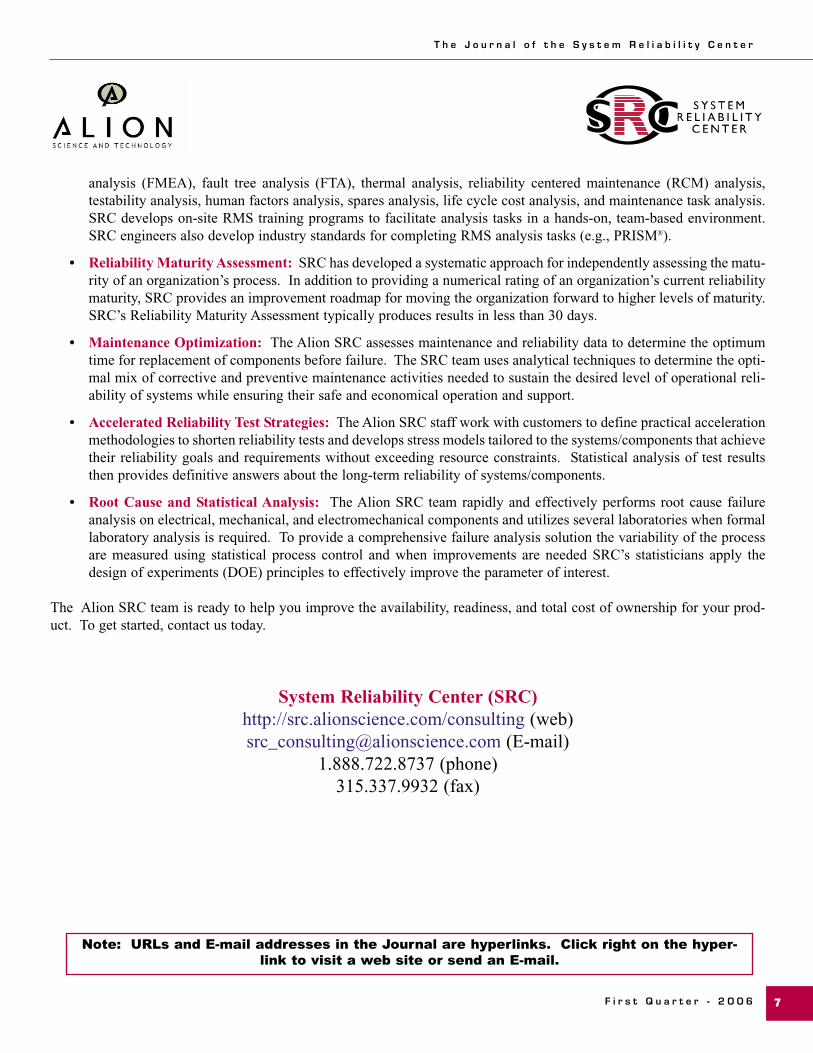
Abrasive Wear Gouging, grinding and scratching are examples of abrasive wear,which occurs when a solid surface experiences the displacementor removal of material as a result of a forceful interaction withanother surface or particle. Particles can become trapped inbetween the two surfaces in contact, and the relative motionbetween them results in abrasion (displacement and removal ofsurface material) of the surface that has a lower hardness. Thisprocess is demonstrated in Figure 2. Sources of particles caninclude foreign contaminants (particles originating outside thesystem), wear debris, or solid constituents suspended in a fluid.Alternatively, abrasive wear can occur in the absence of looseparticles when the roughness of one surface causes abrasionand/or removal of material from the other surface. This wearmechanism differs from adhesive wear in that there is no atomicbonding between the two surfaces. Abrasive erosion occurs whena fluid carrying solid particles is traveling in a direction parallel(as opposed to perpendicular which is impact wear) to the sur-face, and the particles gradually deteriorate the material’s surface.
Figure 2. Illustration of Abrasive Wear Mechanism (Reference 3)
Galling and Seizure Galling is an extreme form of adhesive wear that involves exces-sive friction between the two surfaces resulting in localizedsolid-phase welding and subsequent spalling of the mated parts.This process causes significant damage to the surface of one orboth materials. Seizure is even more extreme in that the two sur-faces experience a sufficient amount of solid-phase welding suchthat the two components can no longer move.
Material hardness is a critical factor in the abrasive wear rate of thesurface, as higher hardness results in a lower wear rate. Moreover,if the hardness of the material’s surface is higher than the hardnessof the abrading particles, then little wear is observed and the parti-cles are likely to be broken into smaller pieces. Materials withhigh hardness and toughness properties are well-suited to preventor minimize abrasive wear. Examples of materials that are inher-ently resistant to abrasive wear include high hardness or surfacehardened steels, cobalt alloys and ceramics. (Reference 3)
Corrosive Wear When the effects of corrosion and wear are combined, a morerapid degradation of the material’s surface may occur. Thisprocess is known as corrosive wear. Films or coatings are often
used to protect a base metal or alloy from harsh environments thatwould otherwise cause it to corrode. If such a coating were sub-jected to abrasive or adhesive wear causing a loss of coating fromthe material’s surface, for instance, the base metal or alloy couldbe exposed and consequently corroded. Alternatively, a surfacethat is corroded or oxidized may be mechanically weakened andmore likely to wear at an increased rate. Furthermore, corrosionproducts including oxide particles that are dislodged from thematerial’s surface can subsequently act as abrasive particles.
Surface Fatigue Wear Surface or contact fatigue occurs when two material surfaces thatare in contact with each other in a rolling or combined rollingand sliding motion create an alternating force or stress orientedin a direction normal to the surface. The contact stress initiatesthe formation of cracks slightly beneath the surface, which thengrow back toward the surface causing pits to form, as particles ofthe material are ejected or worn away. This form of fatigue iscommon in applications where an object repeatedly rolls acrossthe surface of a material resulting in a high concentration ofstress at each point along the surface. For example, rolling-ele-ment bearings, gears, and railroad wheels commonly exhibit sur-face fatigue (References 3 and 6). Figure 3 illustrates an exam-ple of the surface fatigue mechanism.
Figure 3. Illustration of Surface Fatigue Mechanism(Reference 3)
Impact Wear Impact wear is discussed in the section addressing impact failuremodes.
Fretting Wear Surfaces that are in intimate contact with each other and are subjectto a small amplitude relative motion that is cyclic in nature, such asvibration, tend to incur wear. Fretting wear is normally accompa-nied by the corrosion or oxidization of the debris and worn surface.Unlike normal wear mechanisms only a small amount of the debrisis lost from the system; instead the debris remains within the con-joined surfaces. The mated surfaces essentially exhibit adhesionthrough mechanical bonding, and the oscillatory motion causes thesurface to fragment, thereby creating oxidized debris. If the debrisbecomes embedded in the surface of the softer metal, the wear ratemay be reduced. If the debris remains free at the interface betweenthe two materials the wear rate may be increased. Fatigue cracksalso have a tendency to form in the region of wear, resulting in afurther degradation of the material’s surface. Liquid or solid lubri-
A Brief Tutorial on Impact, ... (Continued from page 5)
Abrasive particle
Asperity
Debris
Debris
Travel
Force/Pressure
Crack origin below surface
Solid
Air
Direction of rotation

T h e J o u r n a l o f t h e S y s t e m R e l i a b i l i t y C e n t e r
F i r s t Q u a r t e r - 2 0 0 6 11
cants (e.g., surface treatments, coatings, etc.), residual stresses(e.g., through shot or laser peening), surface grooving (e.g., toenable the release of debris), and/or appropriate material selectionfor the material pair can help to reduce the effects or prevent theoccurrence of fretting wear (Reference 7).
BrinellingBrinelling can be very basically defined as denting. When alocalized area of a material’s surface is repeatedly impacted or issubjected to a static load that overcomes the material’s yieldstrength causing it to permanently deform, it is considered tohave undergone brinelling. Bearings are often susceptible tofailure by brinelling since an indentation can cause an increase invibration, noise, and heating (Reference 7). Brinelling failurescan be caused by improper handling, such as forcing a bearinginto a housing, by dropping the bearing, or by severe vibrations,such as those produced during ultrasonic cleaning (Reference 8).Selecting a material with a high hardness or taking extra careduring handling and cleaning can help prevent brinelling.
Thermal ShockThermal shock is a failure mechanism that occurs in materials thatexhibit a significant temperature gradient (indicating a sudden anddramatic change in temperature has occurred). For instance, if thetemperature gradient is so large that the material experiences ther-mal stresses (or strains) great enough to overcome its strength, itmay lead to fracture, especially if the material is constrained. Anexample of the consequence of thermal shock is shown in Figure4. Awareness of a system or component’s operating conditionswhen selecting materials is important in order to prevent thermalshock failure from occurring. The designer should choose a mate-rial that has an appropriate thermal conductivity and heat capacityfor the intended environmental conditions. In addition, residualstresses (from shot or laser peening, for example) can help accom-modate thermal stresses that are generated during thermal shock,thereby potentially protecting the material from fracture.
Figure 4. Brittle Fracture of a Ductile Weld Material that IsConstrained – Caused by High Stresses Induced from a Rapid
1000°F Change in Temperature (Photo Courtesy of Sachs,Salvaterra & Associates, Inc.)
Radiation DamageThe space environment is very unfriendly to most materials due toan array of harsh conditions that can easily and rapidly degrade thematerial and/or its properties. Degradation of an exposed material
often comes as a result of the different types of radiation present inspace. Radiation is not limited to the space environment, howev-er, as there are a number of environments and specific applicationsthat subject materials to this damaging energy (Figure 5).
Figure 5. CO2 Laser Used to Study the Energy Incident on theEffects of Radiation on Materials (Reference 9)
High-energy radiation, such as neutrons in a nuclear reactor, candamage almost any material including metals, ceramics, and poly-mers (Reference 3). Typically, when a material is subjected to high-energy radiation its properties are altered through structural muta-tion in order to absorb some of the energy that is incident on thematerial. For instance, when a metal is exposed to neutron radia-tion from a nuclear reactor, atoms in the metal are displaced result-ing in the creation of defects. These defects can diffuse and coa-lesce to create crack initiation sites or can simply leave the metalbrittle and susceptible to failure through another mechanism.Another portion of metal is absorbed and converted to heat. Metalsare often better suited to withstand radiation energy than are ceram-ics. Typically, the ductility, thermal conductivity, and electricalconductivity are negatively impacted when a metal is exposed toradiation (Reference 3). Ceramics are affected by radiation to vary-ing extents depending on the type of inherent bonding (i.e., cova-lent or ionic). Ionically-bonded ceramics experience decreases inductility, thermal conductivity, and optical properties, but the dam-age can be reversed with proper heat treatment (similar to metals).Covalently-bonded ceramics experience similar damage; howeverthe damage is somewhat permanent (Reference 3).
Polymers are especially susceptible to radiation even at lowenergy levels, such as UV radiation. Damage from radiation inpolymers usually manifests itself as cracking. For this reason,polymers have been known for their cracking problems in out-door applications, where they are constantly exposed to UV radi-ation. UV blockers, absorbers, and stabilizers are often added topolymers used for outdoor applications to augment their abilityto withstand incident radiation energy.
CorrosionCorrosion is the deterioration of a metal or alloy and its proper-ties due to a chemical or electrochemical reaction with the sur-rounding environment. The most serious result of corrosion is asystem or component failure. Material failure can occur either
(Continued on page 13)

T h e J o u r n a l o f t h e S y s t e m R e l i a b i l i t y C e n t e r
F i r s t Q u a r t e r - 2 0 0 612
Independent Reliability Maturity Assessment
In today’s competitive global marketplace, profit and return-on-investment depend on effective and efficient design andmanufacturing processes. Effective, efficient reliability design processes result in better products, lower production costs,lower ownership costs, and fewer warranty and liability claims.
Product reliability is an important product characteristic because it:
• Is often cited as the reason customers should prefer one product over another.• Can be an important part of a comprehensive risk management program.• Is related to product safety and, hence, company liability.• Directly affects warranty costs and customer satisfaction.
To make reliability a key product requirement, an organization should first determine where it stands in terms of itsprocesses for designing and manufacturing for reliability.
An effective way to do this is through a reliability maturity assessment (RMA).
• Alion Science and Technology’s System Reliability Center (SRC) has developed and implemented a systematicapproach for independently assessing the maturity of an organization’s process for designing and manufacturing forreliability.
• An RMA evaluates the processes used to design and manufacture for reliability to identify shortcomings in thoseprocesses and provides a road map to improvement.
SRC engineers use documented procedures to ensure that our RMA is systematic, objective, and thorough. Our procedures:
• Identify the specific areas to be examined and how the results of the examination will be evaluated and documented.• Are based on objective evidence, not on hearsay or casual impressions.
SRC’s Reliability Maturity Assessment provides the following benefits to our customers:
• Objective identification of strengths and weaknesses• Benefit of lessons learned from a wide range of industries• A roadmap for improvement
For more information, please contact:
System Reliability CenterAlion Science & Technology
201 Mill StreetRome, NY 13440
Tel: 888.722.8737, Fax: 315.337.9932E-mail: <[email protected]>
T h e J o u r n a l o f t h e S y s t e m R e l i a b i l i t y C e n t e r
F i r s t Q u a r t e r - 2 0 0 6 13
by sufficient material property degradation such that the materi-al is rendered unable to perform its intended function, or by frac-ture that originates from or propagated by corrosive effects.
Uniform/General CorrosionUniform corrosion is a generalized corrosive attack that occursover a large surface area of a material. The result is a thinningof the material until failure occurs. Uniform corrosion can alsolead to changes in surface properties such as increased surfaceroughness and friction, which may cause component failureespecially in the case of moving parts that require lubricity.
In most cases corrosion is inevitable. Therefore, mitigating theeffects of corrosion or reducing the corrosion rate is essential toensuring material longevity. Protecting against uniform corro-sion can often be accomplished through selection of a materialthat is best suited for the anticipated environment. The selectionof materials for uniform corrosion resistance should simply takeinto consideration the susceptibility of the metal to the type ofenvironment that will be encountered.
Aside from selecting a uniform corrosion resistant material, protec-tion schemes such as barrier coatings can be implemented. Organicor metallic coatings should be used wherever feasible. When coat-ings are not used, surface treatments that artificially produce themetal oxide layer prior to exposure to the environment will result ina more uniform oxide layer with a controlled thickness. There arealso surface treatments where additional elements are incorporatedfor corrosion resistance, such as chromium. Also, vapor phaseinhibitors may be used in such applications as boilers to combatcorrosive elements and adjust the pH level of the environment.
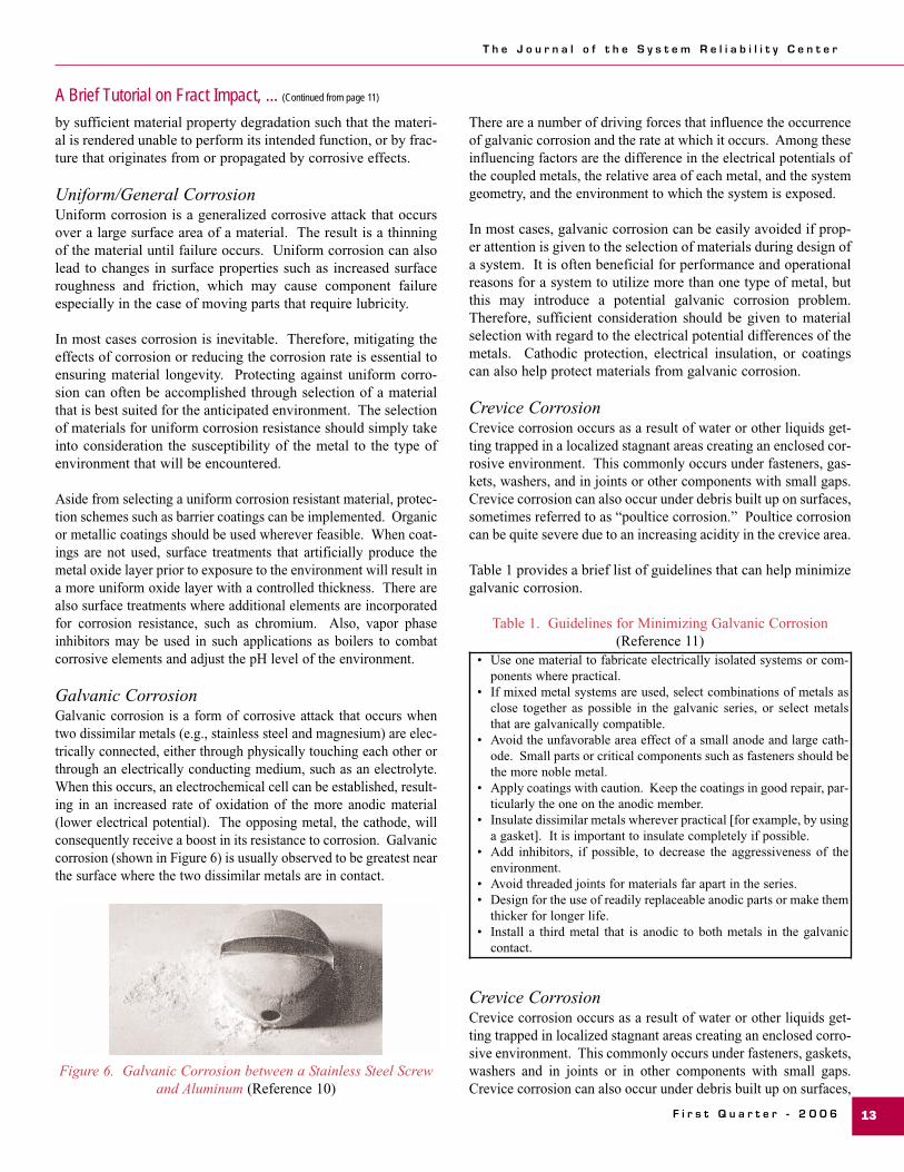
Galvanic CorrosionGalvanic corrosion is a form of corrosive attack that occurs whentwo dissimilar metals (e.g., stainless steel and magnesium) are elec-trically connected, either through physically touching each other orthrough an electrically conducting medium, such as an electrolyte.When this occurs, an electrochemical cell can be established, result-ing in an increased rate of oxidation of the more anodic material(lower electrical potential). The opposing metal, the cathode, willconsequently receive a boost in its resistance to corrosion. Galvaniccorrosion (shown in Figure 6) is usually observed to be greatest nearthe surface where the two dissimilar metals are in contact.
Figure 6. Galvanic Corrosion between a Stainless Steel Screwand Aluminum (Reference 10)
There are a number of driving forces that influence the occurrenceof galvanic corrosion and the rate at which it occurs. Among theseinfluencing factors are the difference in the electrical potentials ofthe coupled metals, the relative area of each metal, and the systemgeometry, and the environment to which the system is exposed.
In most cases, galvanic corrosion can be easily avoided if prop-er attention is given to the selection of materials during design ofa system. It is often beneficial for performance and operationalreasons for a system to utilize more than one type of metal, butthis may introduce a potential galvanic corrosion problem.Therefore, sufficient consideration should be given to materialselection with regard to the electrical potential differences of themetals. Cathodic protection, electrical insulation, or coatingscan also help protect materials from galvanic corrosion.
Crevice CorrosionCrevice corrosion occurs as a result of water or other liquids get-ting trapped in a localized stagnant areas creating an enclosed cor-rosive environment. This commonly occurs under fasteners, gas-kets, washers, and in joints or other components with small gaps.Crevice corrosion can also occur under debris built up on surfaces,sometimes referred to as “poultice corrosion.” Poultice corrosioncan be quite severe due to an increasing acidity in the crevice area.
Table 1 provides a brief list of guidelines that can help minimizegalvanic corrosion.
Table 1. Guidelines for Minimizing Galvanic Corrosion(Reference 11)
Crevice CorrosionCrevice corrosion occurs as a result of water or other liquids get-ting trapped in localized stagnant areas creating an enclosed corro-sive environment. This commonly occurs under fasteners, gaskets,washers and in joints or in other components with small gaps.Crevice corrosion can also occur under debris built up on surfaces,
A Brief Tutorial on Fract Impact, ... (Continued from page 11)
• Use one material to fabricate electrically isolated systems or com-ponents where practical.
• If mixed metal systems are used, select combinations of metals asclose together as possible in the galvanic series, or select metalsthat are galvanically compatible.
• Avoid the unfavorable area effect of a small anode and large cath-ode. Small parts or critical components such as fasteners should bethe more noble metal.
• Apply coatings with caution. Keep the coatings in good repair, par-ticularly the one on the anodic member.
• Insulate dissimilar metals wherever practical [for example, by usinga gasket]. It is important to insulate completely if possible.
• Add inhibitors, if possible, to decrease the aggressiveness of theenvironment.
• Avoid threaded joints for materials far apart in the series. • Design for the use of readily replaceable anodic parts or make them
thicker for longer life. • Install a third metal that is anodic to both metals in the galvanic
contact.
T h e J o u r n a l o f t h e S y s t e m R e l i a b i l i t y C e n t e r
F i r s t Q u a r t e r - 2 0 0 614
sometimes referred to as “poultice corrosion.” Poultice corrosioncan be quite severe, due to an increasing acidity in the crevice area.
Several factors including crevice gap, depth, and the surfaceratios of materials affect the severity or rate of crevice corrosion.Tighter gaps, for example, have been known to increase the rateof crevice corrosion of stainless steels in chloride environments.The larger crevice depth and greater surface area of metals willgenerally increase the rate of corrosion.
Materials typically susceptible to crevice corrosion include alu-minum alloys and stainless steels. Titanium alloys normallyhave good resistance to crevice corrosion. However, they maybecome susceptible in elevated temperature and acidic environ-ments containing chlorides. Copper alloys can also experiencecrevice corrosion in seawater environments.
To protect against problems with crevice corrosion, systemsshould be designed to minimize areas likely to trap moisture,other liquids, or debris. For example, welded joints can be usedinstead of fastened joints to eliminate a possible crevice. Wherecrevices are unavoidable, metals with a greater resistance tocrevice corrosion in the intended environment should be select-ed. Avoid the use of hydrophilic materials (strong affinity forwater) in fastening systems and gaskets. Crevice areas should besealed to prevent the ingress of water. Also, a regular cleaningschedule should be implemented to remove any debris build up.
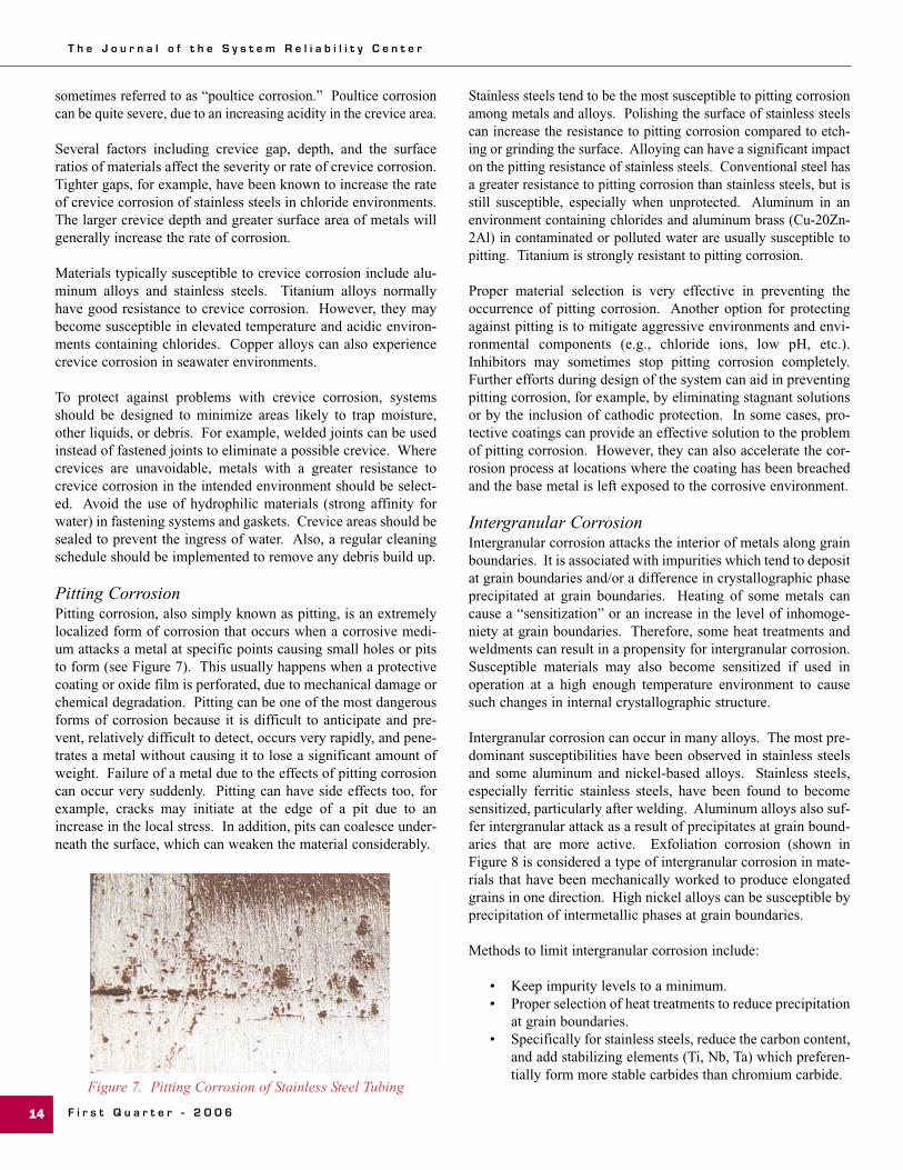
Pitting CorrosionPitting corrosion, also simply known as pitting, is an extremelylocalized form of corrosion that occurs when a corrosive medi-um attacks a metal at specific points causing small holes or pitsto form (see Figure 7). This usually happens when a protectivecoating or oxide film is perforated, due to mechanical damage orchemical degradation. Pitting can be one of the most dangerousforms of corrosion because it is difficult to anticipate and pre-vent, relatively difficult to detect, occurs very rapidly, and pene-trates a metal without causing it to lose a significant amount ofweight. Failure of a metal due to the effects of pitting corrosioncan occur very suddenly. Pitting can have side effects too, forexample, cracks may initiate at the edge of a pit due to anincrease in the local stress. In addition, pits can coalesce under-neath the surface, which can weaken the material considerably.
Figure 7. Pitting Corrosion of Stainless Steel Tubing
Stainless steels tend to be the most susceptible to pitting corrosionamong metals and alloys. Polishing the surface of stainless steelscan increase the resistance to pitting corrosion compared to etch-ing or grinding the surface. Alloying can have a significant impacton the pitting resistance of stainless steels. Conventional steel hasa greater resistance to pitting corrosion than stainless steels, but isstill susceptible, especially when unprotected. Aluminum in anenvironment containing chlorides and aluminum brass (Cu-20Zn-2Al) in contaminated or polluted water are usually susceptible topitting. Titanium is strongly resistant to pitting corrosion.
Proper material selection is very effective in preventing theoccurrence of pitting corrosion. Another option for protectingagainst pitting is to mitigate aggressive environments and envi-ronmental components (e.g., chloride ions, low pH, etc.).Inhibitors may sometimes stop pitting corrosion completely.Further efforts during design of the system can aid in preventingpitting corrosion, for example, by eliminating stagnant solutionsor by the inclusion of cathodic protection. In some cases, pro-tective coatings can provide an effective solution to the problemof pitting corrosion. However, they can also accelerate the cor-rosion process at locations where the coating has been breachedand the base metal is left exposed to the corrosive environment.
Intergranular CorrosionIntergranular corrosion attacks the interior of metals along grainboundaries. It is associated with impurities which tend to depositat grain boundaries and/or a difference in crystallographic phaseprecipitated at grain boundaries. Heating of some metals cancause a “sensitization” or an increase in the level of inhomoge-niety at grain boundaries. Therefore, some heat treatments andweldments can result in a propensity for intergranular corrosion.Susceptible materials may also become sensitized if used inoperation at a high enough temperature environment to causesuch changes in internal crystallographic structure.
Intergranular corrosion can occur in many alloys. The most pre-dominant susceptibilities have been observed in stainless steelsand some aluminum and nickel-based alloys. Stainless steels,especially ferritic stainless steels, have been found to becomesensitized, particularly after welding. Aluminum alloys also suf-fer intergranular attack as a result of precipitates at grain bound-aries that are more active. Exfoliation corrosion (shown inFigure 8 is considered a type of intergranular corrosion in mate-rials that have been mechanically worked to produce elongatedgrains in one direction. High nickel alloys can be susceptible byprecipitation of intermetallic phases at grain boundaries.
Methods to limit intergranular corrosion include:
• Keep impurity levels to a minimum.• Proper selection of heat treatments to reduce precipitation
at grain boundaries.• Specifically for stainless steels, reduce the carbon content,
and add stabilizing elements (Ti, Nb, Ta) which preferen-tially form more stable carbides than chromium carbide.

T h e J o u r n a l o f t h e S y s t e m R e l i a b i l i t y C e n t e r
F i r s t Q u a r t e r - 2 0 0 6 15(Continued on page 18)
Figure 8. Exfoliation of an Aluminum Alloy in a MarineEnvironment
Selective Leaching/DealloyingDealloying, also called selective leaching, is a rare form of corro-sion where one element is targeted and consequently extractedfrom a metal alloy, leaving behind an altered structure. The mostcommon form of selective leaching is dezincification (shown inFigure 9), where zinc is extracted from brass alloys or other alloyscontaining significant zinc content. Left behind are structures thathave experienced little or no dimensional change, but whose par-ent material is weakened, porous and brittle. Dealloying is a dan-gerous form of corrosion because it reduces a strong, ductile metalto one that is weak, brittle and subsequently susceptible to failure.Since there is little change in the metal’s dimensions dealloyingmay go undetected, and failure can occur suddenly. Moreover, theporous structure is open to the penetration of liquids and gasesdeep into the metal, which can result in further degradation.Selective leaching often occurs in acidic environments.
Figure 9. Dezincification of Brass Containing a High ZincContent (Reference 12)
Reducing the aggressive nature of the atmosphere by removingoxygen and avoiding stagnant solutions/debris buildup can pre-vent dezincification. Cathodic protection can also be used forprevention. However, the best alternative, economically, may beto use a more resistant material such as red brass, which onlycontains 15% Zn. Adding tin to brass also provides an improve-ment in the resistance to dezincification. Additionally, inhibitingelements, such as arsenic, antimony and phosphorous can beadded in small amounts to the metal to provide further improve-ment. Avoiding the use of a copper metal containing a signifi-cant amount of zinc altogether may be necessary in systemsexposed to severe dezincification environments.
Erosion CorrosionErosion corrosion is a form of attack resulting from the interactionof an electrolytic solution in motion relative to a metal surface. Ithas typically been thought of as involving small solid particles dis-persed within a liquid stream. The fluid motion causes wear andabrasion, increasing rates of corrosion over uniform (non-motion)corrosion under the same conditions. Erosion corrosion is evidentin pipelines, cooling systems, valves, boiler systems, propellers,impellers, as well as numerous other components. Specializedtypes of erosion corrosion occur as a result of impingement andcavitation. Impingement refers to a directional change of the solu-tion whereby a greater force is exhibited on a surface such as theoutside curve of an elbow joint. Cavitation is the phenomenon ofcollapsing vapor bubbles which can cause surface damage if theyrepeatedly hit one particular location on a metal.
There are several factors that influence the resistance of a materialto erosion corrosion including hardness, surface smoothness, fluidvelocity, fluid density, angle of impact, and the general corrosionresistance of the material to the environment are other propertiesthat factor in. Materials with higher hardness values typicallyresist erosion corrosion better than those that have a lower value.
There are some design techniques that can be used to limit ero-sion corrosion as follow:
• Avoid turbulent flow.• Add deflector plates where flow impinges on a wall.• Add plates to protect welded areas from the fluid stream.
Put piping of concentrate additions vertically into thecenter of a vessel.
Hydrogen DamageThere are a number of different ways that hydrogen can damagemetallic materials, resulting from the combined factors of hydro-gen and residual or tensile stresses. Hydrogen damage can resultin cracking, embrittlement, loss of ductility, blistering and flak-ing, and also microperforation.
Hydrogen induced cracking (HIC) refers to the cracking of aductile alloy when under constant stress and where hydrogen gasis present. Hydrogen is absorbed into areas of high triaxial stressproducing the observed damage. A related phenomenon, hydro-gen embrittlement is the brittle fracture of a ductile alloy duringplastic deformation in a hydrogen gas containing environment.In both cases, a loss of tensile ductility occurs with metalsexposed to hydrogen which results in a significant decrease inelongation and reduction in area. It is most often observed inlow strength alloys and has been witnessed in steels, stainlesssteels, aluminum alloys, nickel alloys, and titanium alloys.
High pressure hydrogen will attack carbon and low-alloy steels athigh temperatures. The hydrogen will diffuse into the metal andreact with carbon resulting in the formation of methane. This in turnresults in decarburization of the alloy and possibly cracks formation.

Relex Reliability Studio 2006
20 years in the making.Relex Reliability Studio 2006
Relex Software is proud to announce the highly
anticipated release of Relex Reliability Studio 2006.
From the company with a history of innovation and a
list of impressive firsts, Relex Reliability Studio does it
once again: redefines reliability engineering tools
with a package of unprecedented power and flexibility
(and a little pizzazz!).

StudioFault Tree/Event Tree
FMEA/FMECA
FRACAS Corrective Acti
Human Factors Risk Ana
Life Cycle Cost
Maintainability Prediction
Markov Analysis
Optimization and Simulation
Reliability Block Diagram
Reliability Prediction
Weibull Analysis
Relex ReliabRelex Reliab
Relex is a registered trademark of Relex Software Corporation. Other brand and product names are trademarks or registered trademarks of their respective holders.
excellence in reliability
Ready to learn more? Check out the Relex trailer at www.relexthemovie.com
and sign up at www.relex.com/news/seminars.asp to attend a preview showing
Studio 2006 – call – 724.836.8800 today!
www.relexthemovie.com See it. Experience it. View the trailer at
Want to see the best in action? With inventive features you hadn’t even
imagined before, our all new Relex Reliability Studio 2006 includes floating,
dockable, and tabbed control windows, the quick configure Relex Bar, the
indispensable Project Navigator, and a completely customizable desktop.
Want global collaboration? The Relex Enterprise Edition supports
both Oracle and SQL Server in a scalable, robust solution with enterprise
capabilities such as permission-based roles, customizable workflow,
alert notifications, audit tracking, and the new Relex iArchitect module
supporting a web browser interface.
T h e J o u r n a l o f t h e S y s t e m R e l i a b i l i t y C e n t e r
F i r s t Q u a r t e r - 2 0 0 618
Methods to deter hydrogen damage are to:
• Limit hydrogen introduced into the metal during processing.• Limit hydrogen in the operating environment.• Structural designs to reduce stresses (below threshold for
subcritical crack growth in a given environment)• Use barrier coatings• Use low hydrogen welding rods
Biological CorrosionMicrobiological corrosion is the acceleration of corrosion due tothe growth or existence of microorganisms in contact with amaterial. This form of corrosion can appear in any environmentcapable of supporting the life of microorganisms and is usually alocalized effect on the metal. Microorganisms may accelerate orimpede corrosion which is attributed to the oxygen concentrationand pH level of the microenvironment. Two types of bacteriaknown to increase corrosion rates are sulfate-reducing bacteriaand sulfate-oxidizing bacteria. Sulfate-reducing bacteria convertsulfates to sulfides which in turn create the metal sulfide corro-sion product. Sulfate-oxidizing bacteria convert sulfate ions toproduce sulfuric acid leading to a decrease in pH level. There arealso many other bacteria capable of producing reduction and oxi-dation type reactions that will affect metals.
Methods to combat microbiological corrosion include:
• Inhibitors/coatings that deter growth of microorganisms.• Preventive maintenance to remove microorganisms.
Stress Corrosion CrackingStress corrosion cracking (SCC) is an environmentally inducedcracking phenomenon that sometimes occurs when a metal issubjected to a tensile stress and a corrosive environment simul-taneously. This is not to be confused with similar phenomenasuch as hydrogen embrittlement, in which the metal is embrittledby hydrogen, often resulting in the formation of cracks.Moreover, SCC is not defined as the cause of cracking thatoccurs when the surface of the metal is corroded resulting in thecreation of a nucleating point for a crack. Rather, it is a syner-gistic effort of a corrosive agent and a modest, static stress.
Another form of corrosion similar to SCC, although with a sub-tle difference, is corrosion fatigue. The key difference is thatSCC occurs with a static stress, while corrosion fatigue requiresa dynamic or cyclic stress.
SCC is a process that takes place within the material, where thecracks propagate through the internal structure, usually leaving thesurface unharmed. Aside from an applied mechanical stress, a resid-ual, thermal, or welding stress along with the appropriate corrosiveagent may also be sufficient to promote SCC. Pitting corrosion,especially in notch-sensitive metals, has been found to be one causefor the initiation of SCC. SCC is a dangerous form of corrosion
because it can be difficult to detect, and it can occur at stress levelswhich fall within the range that the metal is designed to handle.
Stress corrosion cracking is dependent on the environment basedon a number of factors including temperature, solution, metallicstructure and composition, and stress (Reference 13). However,certain types of alloys are more susceptible to SCC in particularenvironments, while other alloys are more resistant to that sameenvironment. Increasing the temperature of a system oftenworks to accelerate the rate of SCC. The presence of chloridesor oxygen in the environment can also significantly influence theoccurrence and rate of SCC. SCC is a concern in alloys that pro-duce a surface film in certain environments, since the film mayprotect the alloy from other forms of corrosion, but not SCC.
There are several methods that may be used to minimize the riskof SCC. Some of these methods include:
• Choose a material that is resistant to SCC.• Employ proper design features for the anticipated forms of
corrosion (e.g., avoid crevices or include drainage holes).• Minimize stresses including thermal stresses.• Environment modifications (pH, oxygen content).• Use surface treatments (shot peening, laser shock peen-
ing) which increase the surface resistance to SCC.• Any barrier coatings will deter SCC as long as it remains
intact.• Reduce exposure of end grains (i.e., end grains can act as
initiation sites for cracking because of preferential corro-sion and/or a local stress concentration).
Corrosion FatigueCorrosion fatigue was discussed in the section addressing fatiguefailure modes.
Failure PreventionIn general, the most effective ways to prevent a material from fail-ing is proper and accurate design, routine and appropriate mainte-nance, and frequent inspection for defects and abnormalities.Each of these general methods will be described in further detail.
Proper design of a system should include a thorough materialsselection process in order to eliminate materials that could poten-tially be incompatible with the operating environment and toselect the material that is most appropriate for the operating andpeak conditions of the system. If a material is selected basedonly on its ability to meet mechanical property requirements, forinstance, it may fail due to incompatibility with the operatingenvironment. Therefore, all performance requirements, operat-ing conditions, and potential failure modes must be consideredwhen selecting an appropriate material for the system.
Routine maintenance will lessen the possibility of a material fail-ure due to extreme operating environments. For example, amaterial that is susceptible to corrosion in a marine environment
A Brief Tutorial on Impact, ... (Continued from page 15)

T h e J o u r n a l o f t h e S y s t e m R e l i a b i l i t y C e n t e r
F i r s t Q u a r t e r - 2 0 0 6 19
could be sustained longer if the salt is periodically washed off. Itis generally a good idea to develop a maintenance plan before thesystem is in service.
Finally, routine inspections can sometimes help identify if amaterial is at the beginning stages of failure. If inspections areperformed in a routine fashion then it is more likely to prevent itfrom failing while the system is in-service.
ConclusionA number of material failure modes were introduced in this articleincluding impact, spalling, wear, brinelling, thermal shock, andradiation damage. These mechanisms can affect metals, polymers,ceramics, and composites in various applications and in many dif-ferent environments. Thus, it is important to take these failuremodes into consideration during the design phases of a componentor system in order to make appropriate materials selection decisions.
From a research standpoint, researchers must consider all materi-al failure modes when developing and maturing a new material orwhen ‘evolving’ an old material. However, material failure canoften be the result of inadequate material selection by the designengineer or their incomplete understanding of the consequencesfor placing specific types of materials in certain environments.
Education and understanding of the nature of materials and howthey fail are essential to preventing it from occurring. Simplefracture or breaking into two pieces is not all-inclusive in terms offailure, because materials also fail by being stretched, dented orworn away. If potential failure modes are understood, then criti-cal systems can be designed with redundancy or with fail-safe fea-tures to prevent a catastrophic failure of the system. Furthermore,if appropriate effort is given to understanding the environment andoperating loads, keeping in mind potential failure modes, then asystem can be designed to be better suited to resist failure.
AcknowledgementThe author would like to thank Neville Sachs and Sachs,Salvaterra & Associates, Inc. for their contribution of photosincluded in this article.
References1. B.D. Craig, Material Failure Modes, Part I: A Brief Tutorial
on Fracture, Ductile Failure, Elastic Deformation, Creep, andFatigue, AMPTIAC Quarterly, Vol. 9, No. 1, AMPTIAC,2005, pages 9-16, <http://amptiac.alionscience.com/pdf/2005MaterialEASE29.pdf>.
2. NASA Spur Gear Fatigue Data, NASA Glenn Research Center,<http://www.grc.nasa.gov/WWW/5900/5950/Fatigue-data.htm>.
3. J.P. Shaffer, A. Saxena, S.D. Antolovich, T.H. Sanders, Jr.,and S.B. Warner, The Science and Design of EngineeringMaterials, 2nd Edition, McGraw-Hill, 1999.
4. P. Niskanen, A. Manesh, and R. Morgan, Reducing Wear WithSuperfinish Technology, AMPTIAC Quarterly, Vol. 7, No. 1,AMPTIAC, 2003, pp.3-9, <http://amptiac.alionscience.com/pdf/AMP Q7_1ART01.pdf>.
5. Wear Failures, Metals Handbook, 9th Edition, Vol. 11:Failure Analysis and Prevention, ASM International, 1986,pp. 145-162.
6. J.R. Davis (editor), ASM Materials Engineering Dictionary,ASM International, 1992.
7. J.A. Collins and S.R. Daniewicz, Failure Modes:Performance and Service Requirements for Metals, M. Kutz(editor), Handbook of Materials Selection, John Wiley andSons, 2002, pp. 705-773.
8. Failures of Rolling-Element Bearings, Metals Handbook,9th Edition, Vol. 11: Failure Analysis and Prevention, ASMInternational, 1986, pp. 490-513.
9. Projects Archive, Air Force Research Laboratory,<http://www.afrl.af. mil/projects.html>.
10. Corrosion Technology Testbed, NASA Kennedy SpaceCenter, <http://corrosion.ksc.nasa.gov/>.
11. E.B. Bieberich and R.O. Hardies, TRIDENT Corrosion ControlHandbook, David W. Taylor Naval Ship Research and Development Center, Naval Sea Systems Command,DTRC/SME-87-99, February 1988; DTIC Doc.: AD-B120 952.
12. Corrosion on Flood Control Gates, U.S. Army Corps of Engi-neers, <http://www.sam.usace.army.mil/en/cp/CORROSION_EXTRA.ppt>.
13. M.G. Fontana, Corrosion Engineering, 3rd Edition, McGraw-Hill, 1986.
System and Part Integrated Data Resource (SPIDRTM) Released April 2006
SPIDR is the NEW Alion SRC comprehensive database of reliabil-ity and test data for systems and components. SPIDR is a revolu-tionary improvement to existing reliability data resources. Withannual updates and twice the volume of data now is the time toupgrade from the four world-renowned data sources: NonelectronicPart Reliability Data (NPRD-95), Electronic Part Reliability Data(EPRD-97), Failure Mode and Mechanism Distributions (FMD-97), and Electrostatic Discharge Susceptibility Data 1995 (VZAP).
SPIDR is a Comprehensive Searchable Database of:
• Over 6,000 unique component types
• System and Component Field Experience Data (>200Krecords of data)
• More than 1016 hours of field reliability data• 33 Different Usage Environments• Environmental and Life Test Data (>82,000 systems and
components)• Electrostatic Discharge (ESD) Susceptibility Data
(>50,000 test results)• Failure Mode and Mechanism Distributions (>27,000
systems and components)• State-of-the-Art Components
(Continued on page 21)
T h e J o u r n a l o f t h e S y s t e m R e l i a b i l i t y C e n t e r
F i r s t Q u a r t e r - 2 0 0 6 21
T h e J o u r n a l o f t h e S y s t e m R e l i a b i l i t y C e n t e r
SPIDR addresses numerous data deficiencies that existed inprior data products. Some examples include:
• Nonelectronic Part Reliability Data (NPRD-95) andElectronic Part Reliability Data (EPRD) • Test data misclassified as field data. SPIDR address-
es this issue and includes a separate database of testdata for components and systems.
• Corrected and improved naming conventions associ-ated with all data. In some instances similar parts haddifferent or incomplete names.
• Reviewed part numbers associated with all data andvalidated that the same name was used for compo-nents with like part number.
• Failure Mode Data (FMD-97)• Failure modes associated with test data were separat-
ed out of SPIDR failure mode distributions. Two sep-arate failure mode data categories exist withinSPIDR, for test and field data.
• Where possible, SPIDR associates a usage environ-ment with failure mode data.
• Failure modes categories were updated. Failure mech-anisms have been separated from failure mode infor-mation. (e.g., prior data products used a failure mech-anism as the failure mode for a given component).
• Electrostatic Discharge Susceptibility Data (VZAP-95)• VZAP-95 includes no data on components manufac-
tured after 1995. SPIDR includes ESD susceptibilitydata for components tested through the end of calen-dar year 2005.
Improvements that you will find in SPIDR:
• More than double the amount of component and system fielddata. SPIDR contains over 1016 hours of field reliabilitydata. (Prior products had a total of only 1012 hours of data).
• Field failure rate data is presented in operational andcalendar hours.
• SPIDR includes the addition of test data for componentsand systems.
• SPIDR includes all “raw data”. SPIDR develops datasummaries based on a user search. Previous data prod-ucts provided predefined data results reducing flexibilityof searches and ease of product and data updates.
• Separate failure mode data resources exist in SPIDR fortest and field data.
• SPIDR provides additional details regarding componentusage. For example SPIDR includes the system applica-tion and the usage environment associated with field andfailure mode data.
• ESD susceptibility data for parts tested and manufacturedafter 1995 are included in SPIDR which more than dou-bles the amount of ESD susceptibility data contained byVZAP-95.
• Improved software interface. Multiple search capabilitiesallow users to find reliability data more efficiently andquickly.
• SPIDR will be updated annually. Prior products wereupdated sporadically.
The cost of SPIDR is $1,995 and data updates are provided annu-ally to maintenance subscribers. The SPIDR software includes auser manual and on-line help to assist the user in understandingthe software capabilities. Visit the SPIDR web site to order yourcopy today and take advantage of the complimentary 1 year ofmaintenance for all SPIDR purchases before June 30, 2006!<http://src.alionscience.com/spidr/>.
If you have additional questions, feel free to contact the SPIDRprogram manager at 315.339.7055 or by E-mail at<[email protected]>.
The iFR Method for Early Prediction of Annualized FailureRate in Fielded Products
By: Bill Lycette, Agilent Technologies
IntroductionAs with many manufacturers of complex electronic equipment,Agilent Technologies uses a non-parametric AFR (AnnualizedFailure Rate) metric for reporting product reliability. However,the AFR metric can be very sluggish in responding to changes incustomer-experienced reliability. When investments to improvereliability culminate in the implementation of an engineeringchange, it can take as many as 9 to 12 months before theimprovement is observed in the AFR. Equally important, degra-dation in reliability may be quickly detected by customers but itmay take several months before a change is observed in the man-ufacturer’s internal AFR measures.
The “instant Failure Rate” (iFR) is a parametric-based measuredeveloped for the express purpose of providing much quicker
feedback of changes in a product’s reliability. This paperexplains the iFR Method through analysis of actual field failuredata and demonstrates how a balance is struck between selectingiFR variables that yield the best possible combination of quickreliability feedback, effective AFR predictive power, and narrowconfidence bounds.
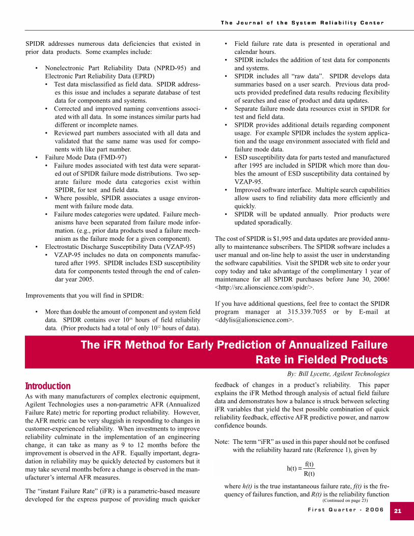
Note: The term “iFR” as used in this paper should not be confusedwith the reliability hazard rate (Reference 1), given by
where h(t) is the true instantaneous failure rate, f(t) is the fre-quency of failures function, and R(t) is the reliability function
(Continued on page 23)
R(t)
f(t) h(t) =

Accuracy
Accuracy
Support
Support
Total
Solution
Total
Solution
Scalability
Scalability
The World’s Most AdvancedRisk Management, Reliability, Availability,
Maintainability and Safety Technology
When you purchase Item products, you are not just buying software - you are expanding your team. Item delivers accuracy, knowledgeable and
dependable support, total solutions and scalability. Let us join your team!
• Solutions and Services • Integrated Software • Education and Training • Consulting
Item ToolKit: • Reliability Prediction • Mil-HDBK-217 (Electronics) • Bellcore / Telcordia (Electronics) • RDF 2000 (Electronics) • China 299b (Electronics) • NSWC (Mechanical) • Maintainability Analysis • SpareCost Analysis • Failure Mode Effect and Criticality Analysis • Reliability Block Diagram • Markov Analysis • Fault Tree Analysis • Event Tree Analysis
Item QRAS: • Quantitative Risk Assessment System • Event Sequence Diagram (ESD) • Binary Decision Diagram (BDD) • Fault Tree Analysis • Sensitivity Analysis • Uncertainty Analysis
Our #1 Mission:Commitment to you and your success
USA East, USA West and UK Regional locations to serve you effectively and efficiently.
Item Software Inc. US: Tel: 714-935-2900 • Fax: 714-935-2911 • [email protected]
UK: Tel: +44 (0) 1489 885085 • Fax: +44 (0) 1489 885065 • [email protected]
www.itemsoft.comwww.itemsoft.com
NowAvailable!
T h e J o u r n a l o f t h e S y s t e m R e l i a b i l i t y C e n t e r
F i r s t Q u a r t e r - 2 0 0 6 23
representing the probability that the product will survive untiltime t. In this paper, “iFR” is meant to signify a metric thatis much more responsive than the non-parametric AFR inmeasuring the reliability of products currently being shipped.
Annualized Failure Rate MetricsA widely-used method for measuring reliability of electronicequipment is calculating field failure rates using the AnnualizedFailure Rate (AFR). There are countless different variations onsuch non-parametric methods as explained in Reference 2, butthey generally rely upon simple calculations involving the num-ber of failures and the size of the installed base (Reference 3).
The advantages of such methods are their simplicity and ease ofunderstanding. No special software or graphing paper is requiredto make the calculation. The computation is straightforward andcan be performed by someone unfamiliar with reliability statis-tics. The calculation is quick, simple and can be easily explainedto the layperson. For these reasons, AFR is widely used in indus-try to measure the reliability of electronic equipment.
The disadvantages of such AFR methods are several. Thesemethods do not allow for quantification of confidence bounds.Additionally, many of such metrics make the potentially falseassumption that the underlying failure rate is constant over time.These methods also do not allow for conditional probability cal-culations.
Finally, a major disadvantage of AFR methods is that they can besluggish to respond to changes in product reliability (both degra-dation and improvement) during the product’s manufacturinglife cycle. The iFR Method provides a solution to sluggishresponse time.
The iFR MethodThe method is based on parametric techniques involving relia-bility statistics and principles. Reliability statistics are well doc-umented in textbooks and the literature (References 4, 5, and 6).
By using the iFR Method, changes in the reliability of complexelectronic measurement equipment can be detected by as manyas four to six months earlier than would be otherwise possibleusing some conventional AFR methods.
Keys to SuccessThe keys to the success of the iFR Method include selecting ashipment evaluation window that strikes the optimum balanceamong the following.
1. Providing timely feedback of reliability changes,2. Detecting the occurrence of new failure mechanisms,3. Providing acceptable confidence bounds,4. Minimizing reliability false alarms, and5. Providing useful predictive power for anticipating even-
tual changes in AFR.
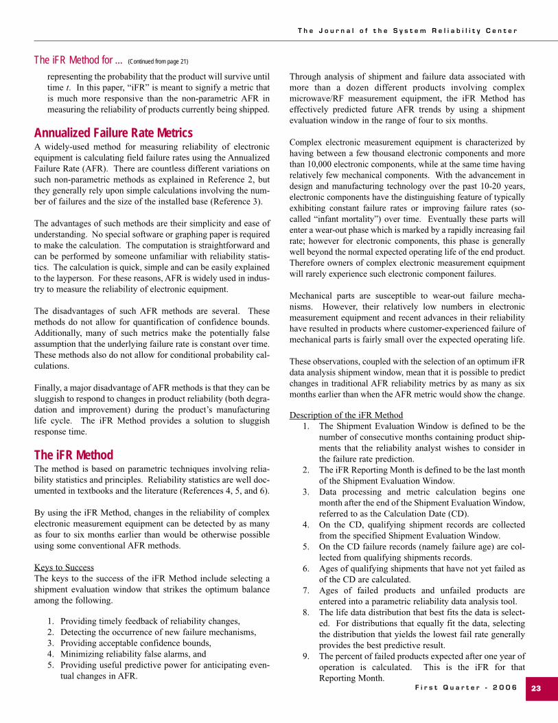
Through analysis of shipment and failure data associated withmore than a dozen different products involving complexmicrowave/RF measurement equipment, the iFR Method haseffectively predicted future AFR trends by using a shipmentevaluation window in the range of four to six months.
Complex electronic measurement equipment is characterized byhaving between a few thousand electronic components and morethan 10,000 electronic components, while at the same time havingrelatively few mechanical components. With the advancement indesign and manufacturing technology over the past 10-20 years,electronic components have the distinguishing feature of typicallyexhibiting constant failure rates or improving failure rates (so-called “infant mortality”) over time. Eventually these parts willenter a wear-out phase which is marked by a rapidly increasing failrate; however for electronic components, this phase is generallywell beyond the normal expected operating life of the end product.Therefore owners of complex electronic measurement equipmentwill rarely experience such electronic component failures.
Mechanical parts are susceptible to wear-out failure mecha-nisms. However, their relatively low numbers in electronicmeasurement equipment and recent advances in their reliabilityhave resulted in products where customer-experienced failure ofmechanical parts is fairly small over the expected operating life.
These observations, coupled with the selection of an optimum iFRdata analysis shipment window, mean that it is possible to predictchanges in traditional AFR reliability metrics by as many as sixmonths earlier than when the AFR metric would show the change.
Description of the iFR Method1. The Shipment Evaluation Window is defined to be the
number of consecutive months containing product ship-ments that the reliability analyst wishes to consider inthe failure rate prediction.
2. The iFR Reporting Month is defined to be the last monthof the Shipment Evaluation Window.
3. Data processing and metric calculation begins onemonth after the end of the Shipment Evaluation Window,referred to as the Calculation Date (CD).
4. On the CD, qualifying shipment records are collectedfrom the specified Shipment Evaluation Window.
5. On the CD failure records (namely failure age) are col-lected from qualifying shipments records.
6. Ages of qualifying shipments that have not yet failed asof the CD are calculated.
7. Ages of failed products and unfailed products areentered into a parametric reliability data analysis tool.
8. The life data distribution that best fits the data is select-ed. For distributions that equally fit the data, selectingthe distribution that yields the lowest fail rate generallyprovides the best predictive result.
9. The percent of failed products expected after one year ofoperation is calculated. This is the iFR for thatReporting Month.
The iFR Method for ... (Continued from page 21)
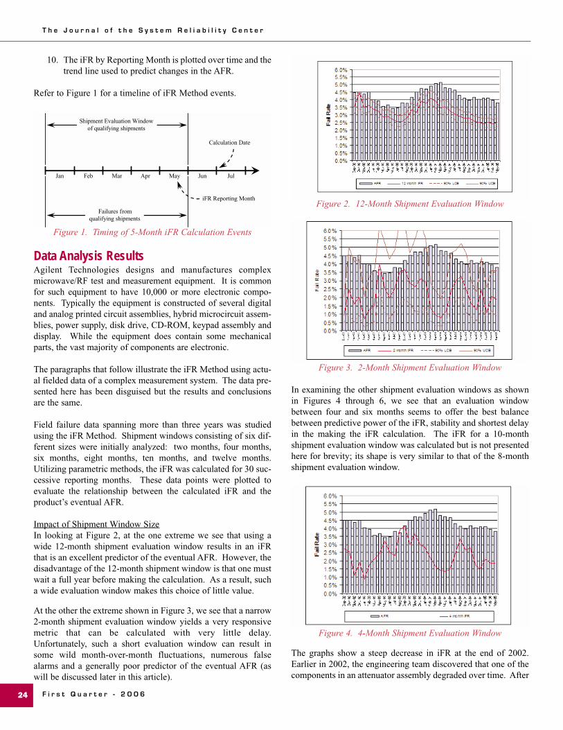
T h e J o u r n a l o f t h e S y s t e m R e l i a b i l i t y C e n t e r
F i r s t Q u a r t e r - 2 0 0 624
10. The iFR by Reporting Month is plotted over time and thetrend line used to predict changes in the AFR.
Refer to Figure 1 for a timeline of iFR Method events.
Figure 1. Timing of 5-Month iFR Calculation Events
Data Analysis ResultsAgilent Technologies designs and manufactures complexmicrowave/RF test and measurement equipment. It is commonfor such equipment to have 10,000 or more electronic compo-nents. Typically the equipment is constructed of several digitaland analog printed circuit assemblies, hybrid microcircuit assem-blies, power supply, disk drive, CD-ROM, keypad assembly anddisplay. While the equipment does contain some mechanicalparts, the vast majority of components are electronic.
The paragraphs that follow illustrate the iFR Method using actu-al fielded data of a complex measurement system. The data pre-sented here has been disguised but the results and conclusionsare the same.
Field failure data spanning more than three years was studiedusing the iFR Method. Shipment windows consisting of six dif-ferent sizes were initially analyzed: two months, four months,six months, eight months, ten months, and twelve months.Utilizing parametric methods, the iFR was calculated for 30 suc-cessive reporting months. These data points were plotted toevaluate the relationship between the calculated iFR and theproduct’s eventual AFR.
Impact of Shipment Window SizeIn looking at Figure 2, at the one extreme we see that using awide 12-month shipment evaluation window results in an iFRthat is an excellent predictor of the eventual AFR. However, thedisadvantage of the 12-month shipment window is that one mustwait a full year before making the calculation. As a result, sucha wide evaluation window makes this choice of little value.
At the other the extreme shown in Figure 3, we see that a narrow2-month shipment evaluation window yields a very responsivemetric that can be calculated with very little delay.Unfortunately, such a short evaluation window can result insome wild month-over-month fluctuations, numerous falsealarms and a generally poor predictor of the eventual AFR (aswill be discussed later in this article).
Figure 2. 12-Month Shipment Evaluation Window
Figure 3. 2-Month Shipment Evaluation Window
In examining the other shipment evaluation windows as shownin Figures 4 through 6, we see that an evaluation windowbetween four and six months seems to offer the best balancebetween predictive power of the iFR, stability and shortest delayin the making the iFR calculation. The iFR for a 10-monthshipment evaluation window was calculated but is not presentedhere for brevity; its shape is very similar to that of the 8-monthshipment evaluation window.
Figure 4. 4-Month Shipment Evaluation Window
The graphs show a steep decrease in iFR at the end of 2002.Earlier in 2002, the engineering team discovered that one of thecomponents in an attenuator assembly degraded over time. After
Failures from qualifying shipments
Shipment Evaluation Window of qualifying shipments
Jan Feb Mar Apr Jun May Jul
iFR Reporting Month
Calculation Date

T h e J o u r n a l o f t h e S y s t e m R e l i a b i l i t y C e n t e r
F i r s t Q u a r t e r - 2 0 0 6 25
evaluating alternative components, an improved device wasselected and implemented in mid-2002. To the engineeringteam’s relief, the AFR subsequently dropped as predicted by theiFR and the design change was affirmed.
Figure 5. 6-Month Shipment Evaluation Window
Figure 6. 8-Month Shipment Evaluation Window
The initial increase in iFR throughout the first half of 2003 accu-rately predicted an associated increase in AFR during the secondhalf of 2003. A Pareto analysis of failed assemblies showedincreasing failure rates of several printed circuit assemblies (PCA).Failure analysis of the PCAs revealed a fabrication problem withtantalum capacitors purchased from the same supplier. Other sup-pliers’ components were evaluated and devices with improved reli-ability implemented later in 2003. The iFR gave advance notice ofthe problem and confirmed that the solution would be effective.
To further optimize predictive results, the iFR Method wasrefined by calculating failure rates using a 5-month shipmentevaluation window. The results are shown in Figure 7.
Confidence BoundsAnother important aspect when considering what size of evalua-tion period to select is the width of the iFR confidence bounds.Confidence bounds on failure rates are inversely proportional tothe number of field failures observed.
Consequently, narrowest confidence bounds will occur with thelargest shipment evaluation windows.
Figure 7. 5-Month Shipment Evaluation Window
For a failure process that follows the exponential distribution,the two-sided upper limit on the failure rate is:
where χ2 is the Chi square distribution, α is the significancelevel, 2r+2 is the degrees of freedom (r is the number of failuresobserved) and T is the total product exposure time.4
The two-sided lower limit on the failure rate is given by:
Larger shipment evaluation windows will provide greater preci-sion in the metric. Again, we have the tradeoff between usingsmall shipment windows (quick reliability feedback) and largershipment windows. The effect of evaluation window size onconfidence bounds can be seen in Figures 2 and 3.
The confidence bounds for shipment evaluation windows of fourmonths, five months and six months were also calculated (notpresented here for brevity). These confidence bounds were allroughly the same and therefore did not play a significant factorin selecting the optimum shipment evaluation window.
iFR Predictive PowerWe want a shipment evaluation period that affords the best pos-sible predictive power (using iFR to predict the eventual AFR)while at the same time minimizing calculation delay time andconfidence bound widths. A correlation analysis using linearregression was performed where iFR and eventual AFR werecompared using the previously described shipment evaluationwindows. For each shipment evaluation window, correlationcoefficients were calculated using five different iFR lead times.iFR lead time represents the amount of advance notice that theiFR metric provides with respect to predicting the eventual AFRnumber. Analysis results are shown in Table 1.
Similar to a long range weather forecast, iFR predictive accura-cy declines as we attempt to predict further into the future about
2T
22 ,2r 2/
U+αχ
=λ
2T
2,2r2/ - 1
Lαχ
=λ

T h e J o u r n a l o f t h e S y s t e m R e l i a b i l i t y C e n t e r
F i r s t Q u a r t e r - 2 0 0 626
what the AFR will eventually be. We also see that the iFR pre-dictive power improves with larger shipment evaluation win-dows. Larger evaluation windows tend to yield better resultsbecause 1) greater customer-use time (i.e., exposure time) pro-vides for more latent failure mechanisms to manifest themselves,and 2) larger data sets drive smaller random variation (confi-dence bounds) in the calculated iFR.
Table 1. Correlation Coefficients to Assess the PredictivePower of the iFR
It would make little sense to use a shipment evaluation windowof 10 or 12 months because one would have to wait for nearlyone year in order to make an accurate statement about what theAFR is likely to do in the following month.
In this example, we see that the sweet spot for predicting AFR(highest predictive power, shortest iFR calculation delay andacceptable confidence bounds) is achieved by selecting a fivemonth shipment evaluation window. This results in an optimumAFR lead time indicator of four months. Slightly inferior, butnevertheless useful, results can be obtained with four and sixmonth shipment evaluation windows.
LimitationsMethods for predicting field failure rates are based on failuremechanisms that have already manifested themselves. If a spe-cific failure mechanism, e.g., the wear out of a disk drive bear-ing, has not already presented itself in the data, then such meth-ods have no way of knowing that the failure mechanism canoccur. As such, predictive methods would not be effective onproducts that have failure mechanisms occurring beyond theedge of the shipment evaluation window.
While complex electronic measurement equipment is typicallyconstructed of electronic components that exhibit constant ordecreasing failure rates, there are occasions when such compo-nents may exhibit an increasing failure rate during the product’snormal expected operating life. Likewise, one of the product’shandful of mechanical parts may enter a wear out phase unex-pectedly early. Either of these two scenarios would likely notprovide for an accurate AFR prediction based on only a fewmonths of early field data used in the iFR Method.
ConclusionsReliability metrics such as the widely used Annualized FailureRate can be extremely sluggish to respond to changes in the prod-
uct’s reliability over the course of its manufacturing life cycle.The iFR Method described in this paper has been shown to beeffective in providing a more responsive leading indicator of cus-tomer-experienced reliability in complex electronic equipment.
Waiting six, nine or even 12 months for a reliability problem to bereflected in traditional AFR metrics represents a huge delay insolving the root cause of the problem. In the mean time, shipmentsof the problem continue thus increasing the installed base and asso-ciated exposure to higher warranty costs, greater customer dissat-isfaction and lost future sales. Additionally, it is costly and frus-trating to wait long periods of time to determine if a recently-implemented fix was actually successful. Metrics such as AFR areslow to reflect the effectiveness of such a fix, and several monthsof patiently monitoring the AFR may give way to making costly,unnecessary investments in additional reliability improvements.
The iFR Method provides timely, valuable feedback to manufac-turers thus enabling them to 1) quickly take action in response todegradation in product reliability, and 2) avoid costly, unneces-sary engineering changes when recent improvements are judgedto be effective and adequate.
References1. Reliability Engineering Handbook, Volume 1, Dimitri
Kececioglu, Prentice-Hall, 1991.2. “AFR: Problems of Definition, Calculation and
Measurement in a Commercial Environment”, J.G. Elerath,Reliability and Maintainability Symposium AnnualProceedings, January 24-27 2000, pp. 71-76.
3. IEEE Guide for Selecting and Using Reliability PredictionsBased on IEEE 1413™, The Institute of Electrical andElectronics Engineers Inc, 2003.
4. Applied Reliability, Second Edition, Paul A. Tobias andDavid C. Trindade, CRC Press, 1995.
5. Practical Reliability Engineering, Fourth Edition, PatrickD.T. O’Connor, John Wiley & Sons, Inc., 2002.
6. “Practical Considerations in Calculating Reliability ofFielded Products”, Bill Lycette, The Journal of the RAC,Second Quarter 2005, pp. 1-6.
About the AuthorBill Lycette is a Senior Reliability Engineer with AgilentTechnologies. He has 25 years of engineering experience withHewlett-Packard and Agilent Technologies, including positionsin reliability and quality engineering, process engineering, andmanufacturing engineering of microelectronics, printed circuitassemblies and system-level products. Mr. Lycette is an ASQCertified Reliability Engineer and Certified Quality Engineer.
Shipment WindowSize (in Months)
AFR Advance Warning Lead Time (in months)0 1 2 3 4 5 6 7 8
2 - - - - 0.48 0.57 0.59 0.47 0.344 - - - 0.53 0.67 0.68 0.65 0.53 -5 - - 0.55 0.74 0.79 0.70 0.60 - -6 - 0.39 0.60 0.71 0.68 0.53 - - -8 0.45 0.58 0.70 0.64 0.49 - - - -10 0.71 0.69 0.72 0.62 - - - - -12 0.71 0.67 0.61 - - - - - -

T h e J o u r n a l o f t h e S y s t e m R e l i a b i l i t y C e n t e r
F i r s t Q u a r t e r - 2 0 0 6 27
How Did I Get Here!I’ve heard it said that life is a funny dog. It takes some twists andturns that we can neither plan nor expect. So in looking back onone’s career, it is not surprising that we find our careers havetaken a twisty path.
I did not choose to be a reliability engineer – that career path sortof chose me. While I was a First Lieutenant in the United StatesAir Force, stationed at Wright-Patterson AFB and working ontest bed modifications, I was centrally selected for the SystemsEngineering-Reliability Master’s Degree program at the AirForce Institute of Technology. At the time, I had never heard ofreliability and had planned to get my Master’s Degree in thesame area as my Bachelor’s Degree – Mechanical Engineering.However, a Master’s Degree at Government expense is nothingto turn down. So I accepted the opportunity.
That was nearly 37 years ago. In those three plus decades, I havecome to be an avid and enthusiastic supporter of the reliabilityand related disciplines. Like my colleagues in the field, I knowthat understanding the causes of failure and taking action to mit-igate or prevent those failures, first through design changes andlater through improvements in production, operation, or mainte-nance, is vital to the defense of our country and the economicvitality of our economy.
Like many of my colleagues, I also have come to realize that reli-ability is not consistently or even readily embraced by managersand those holding the purse strings. In part, this reluctance toaccept reliability as a necessary performance parameter is due tothe probabilistic nature of reliability and our inability to forecastprecisely when a failure will occur or how many failures willoccur in a given interval of time.
Another reason reliability is not a top priority with managers isthat the benefits of a robust reliability program are long term andnot seen until after a product is sold or a system is fielded. Thecosts, however, are immediate. Training, reliability softwaretools, growth testing, redesign, data collection, root cause failureanalysis, and other essential reliability tasks require resourcestoday, not tomorrow.
Consequently, as a result of these two reasons and a third which Iwill touch upon in a minute, much of my reliability career, andthose of many of my colleagues, has been spent in trying to “sell”reliability to management. As a proponent, I have expounded onthe long-term benefits of reliability and the costs and risks incurredby ignoring reliability. I have worked to educate managers andengineers in the reliability discipline, trying to dispel the manymyths that surround the subject. I have had some success but notnearly as much as I would have liked or I think is needed.
Those who know me well know my thirdreason for this unsatisfactory level ofsuccess in making reliability a part ofevery program. They know that I lay theblame on our society’s penchant forimmediate gratification. Whether it beadult stockholders or teenage children,members of our society seem unable tolook much beyond tomorrow. Why savefor the future when we can spend today,even if it means living on credit? Whyinvest in our companies to help ensuretheir future and that of the employeeswhen we can make huge profits today tokeep the stockholders happy?
Reliability requires looking to the future, not dwelling on the pres-ent. Reliability requires that one recognizes that “you must pay nowor pay even more later.” Many a system has required considerableinvestment of resources to achieve a reasonable level of availabilityduring its operational life, simply because little or no attention wasdevoted to reliability during acquisition and production.
Perhaps some of our readers have similar stories and perceptionsregarding their career in reliability. And despite the times thatwe have failed to convince managers to spend money now tosave money, reduce risks, and increase performance later, wepersevere. We persevere because we believe in what we aredoing. We persevere because we have seen the dire conse-quences of neglecting a basic part of system engineering. Theseconsequences are, unfortunately, not limited to higher costs.They include loss of life, injury, unsuccessful military missions,and gut-wrenching scenes of a space vehicle self-destructing inthe clear blue skies over Florida.
Many may regard the passion that reliability engineers bring totheir job as overdone or excessive. We are too focused, theycomplain, and too zealous. Perhaps. But I think that everyonewhose life depends on the reliable operation of a system may seeus in a different light.
Reliability engineers may not receive the recognition or creditgiven to those in other branches of engineering. However,recognition and credit are not the reasons I have stayed in theprofession and I doubt they are what motivate my colleagues.
I may have started down the path of reliability engineering byaccident. But I have stayed the course on purpose. I have takenand continue to take great pride in the work that my colleaguesand I do. I know how I got here and I know why I stayed.
Ned H. Criscimagna
From the Editor
The appearance of advertising in this publication does not constitute endorsement by SRCof the products or services advertised.
T h e J o u r n a l o f t h e S y s t e m R e l i a b i l i t y C e n t e rT h e J o u r n a l o f t h e S y s t e m R e l i a b i l i t y C e n t e r
For a complete listing of upcomingRMS events, click on
the following link:<http://src.alionscience.com/
calendar>
2006 DoD Standardization ConferenceMay 23-25, 2006Arlington, VAContact: Nancy EibenSAE InternationalSAE World Headquarters400 Commonwealth DriveWarrendale, PA 15096-0001Tel: 724.772.8525Fax: 724.776.1830E-mail: <[email protected]>On the Web: <http://www.sae.org/
events/dsp/>
Safety 2006June 11-14, 2006Seattle, WAContact: The American Society of Safety
EngineersCustomer Service1800 E Oakton StreetDes Plaines, IL 60018 Tel: 847.699.2929Fax: 847.768.3434E-mail: <[email protected]>On the Web: <http://www.safety2006.org>
2006 International Applied Reliability Symposium
June 14-17, 2006Orlando, FLContact: Patrick HetheringtonAlion System Reliability Center201 Mill StreetRome, NY 13440Tel: 315.339.7084Fax: 315.337.9932E-mail: <[email protected]>On the Web: <http://www.arsymposium.
org>
Human Factors in DefenceJune 14-15, 2006Contact: Horun MeahSMi Group Ltd, Unit 009Great Guildford Business Square30 Great Guildford StreetLondon SE1 0HSUnited KingdomTel: 44.0.20.7827.6192Fax: 44.0.20.7827.6001E-mail: <[email protected]>On the Web: <http://www.smi-online.co.
uk/events/overview.asp?is=1&ref=2348>
CMMI Technology Conference & Users Group
November 13-16, 2006Denver, COContact: Emily BrownNDIAArlington, VA 22201-3061 Tel: 703.247.9476Fax: 703.522.1885E-mail: <[email protected]> On the Web: <http://www.ndia.org/
Template.cfm?Section=7110&Template=/ContentManagement/ContentDisplay.cfm&ContentID=10838>
Future Events in Reliability, Maintainability, and Supportability