CADMIUM JUMP FREQUENCIES IN L12

INTERMETALLIC COMPOUNDS

By

XIA JIANG

A thesis submitted in partial fulfillment of the requirements for the degree of

MASTER OF SCIENCE IN PHYSICS

WASHINGTON STATE UNIVERSITY Department of Physics and Astronomy

May 2008

ii

To the Faculty of Washington State University:

The members of the Committee appointed to examine the thesis of XIA JIANG find it satisfactory and recommend that it be accepted.

___________________________________ Chair ___________________________________ ___________________________________

iii

ACKNOWLEDGMENTS

I am grateful to Prof. Gary S. Collins for introducing me into the field of nuclear

condensed matter physics, for his guidance in the selection of research topics and the

interpretation of experimental results, and for his patience in answering my many

questions.

I would like to thank Prof. Matthew O. Zacate for his helpful comments on jump

mechanisms.

My thanks go to John Bevington for his help with sample preparation and data

processing, and for sharing his expertise on the instruments. I owe my thanks to Randal

Newhouse for his kind help with experiments.

I would also like to thank Arriety Lowell, , Benjamin Norman and Justin Ann for

the constructive discussions with them.

This work is supported in part by the National Science Foundation under grant

DMR 05-04843 (Metals Program)

iv

CADIMIUM JUPM FREQUENCIES IN L12

INTERMETALLIC COMPOUNDS

Abstract

by Xia Jiang, M.S.

Washington State University May 2008

Chair: Gary S. Collins

Perturbed angular correlation spectroscopy was applied to study atomic

movement in L12 type rare earth indides, gallides and aluminides. Nuclear relaxations

were measured as a function of temperature and were related to the jump frequencies of

111In/Cd tracers by the XYZ model. Activation enthalpies were obtained by fitting jump

frequencies to the Arrhenius temperature dependence. Measurements were made on

opposing phase boundaries of the indide phases and the jump frequency was found to be

highly dependent on the composition of the samples. Higher jump frequency and lower

activation enthalpy were observed at the more In-rich phase boundary for the early rare

earth indides and at the less In-rich phase boundary for the late rare earth indides. This

reversal of behavior strongly suggests the existence of different diffusion mechanisms.

The behavior of the late rare earth indides can be explained by a simple monovacancy

diffusion mechanism. Three mechanisms are discussed in order to explain the behavior

of the early rare earth indides, among which the six jump cycle mechanism is decided to

be the most feasible one. With the assumption of this mechanism, the differences

between activation enthalpies for the opposing phase boundaries are attributed to

formation enthalpies of rare earth vacancies.

v

TABLE OF CONTENTS

Acknowledgements...................................................................................................... iii

Abstract .........................................................................................................................iv

List of figures.............................................................................................................. vii

List of tables............................................................................................................... viii

1. Introduction................................................................................................................1

2. Theory ........................................................................................................................4

2.1 Perturbed angular correlation spectroscopy......................................................4

2.1.1 Spin alignment and unperturbed angular correlation of gamma-rays.....4

2.1.2 Spin precession and perturbed angular correlation of gamma-rays........5

2.1.3 Electric quadrupole interaction of 111In/111Cd.........................................6

2.1.4 Dynamic perturbation function and the XYZ model ..............................9

2.1.5 Inhomogeneous broadening ..................................................................10

2.2 Diffusion mechanisms and point defects in L12 phases..................................10

3. Experimental methods .............................................................................................15

3.1 PAC instrumentation .......................................................................................15

3.2 Data reduction.................................................................................................17

3.3 Sample preparation .........................................................................................18

3.4 Measurement at high temperature...................................................................20

4. Results......................................................................................................................21

4.1 PrIn3 ................................................................................................................21

vi

4.2 NdIn3 ...............................................................................................................26

4.3 TmIn3 ..............................................................................................................29

4.4 GdIn3 ...............................................................................................................31

4.5 DyGa3, ErGa3, LuGa3 and ErAl3.....................................................................32

5. Discussion ................................................................................................................35

5.1 Cd jump frequencies in various L12 intermetallics.........................................35

5.2 Actual compositions of the A and B phase boundaries ...................................39

5.3 Diffusion mechanisms.....................................................................................41

6. Summary ..................................................................................................................47

References....................................................................................................................49

vii

LIST OF FIGURES

Fig. 1. Unit cell of L12 type A3B phase ........................................................................... 2

Fig. 2. Angular correlation of two gamma-ray emissions. .............................................. 5

Fig. 3. Decay scheme of 111In .......................................................................................... 6

Fig. 4. Energy splitting of the 5 / 2I = intermediate state............................................. 8

Fig. 5. Scheme of B-vacancy six jump cycle mechanism ............................................. 12

Fig. 6. Scheme of 3-ring and 4-ring diffusion in fcc metals.......................................... 13

Fig. 7. Diagram of PAC electronics............................................................................... 16

Fig. 8. Coincidence rate curve of 111In/Cd in ferromagnetic iron.................................. 17

Fig. 9. Phase diagram of Pr-In system........................................................................... 21

Fig. 10. PAC spectra of PrIn3. ....................................................................................... 23

Fig. 11. Arrhenius plot of Cd jump frequencies in PrIn3............................................... 25

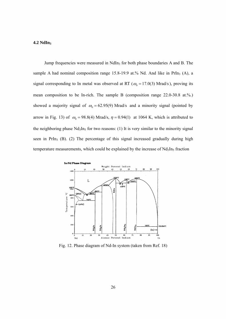
Fig. 12. Phase diagram of Nd-In system ....................................................................... 26

Fig. 13. PAC spectra of NdIn3. ...................................................................................... 27

Fig. 14. Arrhenius plot and of Cd jump frequencies in NdIn3....................................... 28

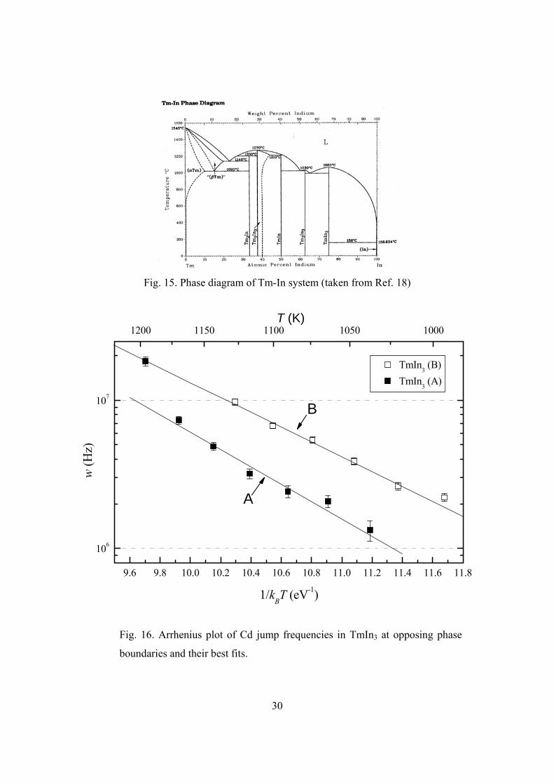
Fig. 15. Phase diagram of Tm-In system....................................................................... 30

Fig. 16. Arrhenius plot of Cd jump frequencies in TmIn3............................................. 30

Fig. 17. Arrhenius plot of Cd jump frequencies in GdIn3............................................. 31

Fig. 18. PAC spectra of ErGa3....................................................................................... 32

Fig. 19. Arrhenius plot and of Cd jump frequencies in DyGa3, ErGa3, LuGa3 and

ErAl3. ..................................................................................................................... 34

Fig. 20. Cd jump frequencies in L12 intermetallics....................................................... 36

viii

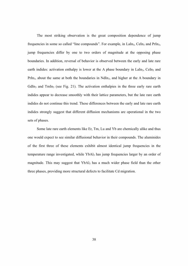
Fig. 21 Activation enthalpies of Cd jump in RIn3 systems vs. lattice parameters......... 39

Fig. 22. Determination of phase boundaries of RIn3 using free energy curves............. 40

LIST OF TABLES

Table 1. Prefactors and activation enthalpies for Cd jump in various L12 phases.. .37

Table 2. Formation enthalpies of thermal defects in RIn3 ........................................46

1

1. Introduction

Diffusion in solids has traditionally been studied by using radioactive tracers and

depth profiling techniques. More recently, it has also been studied on a microscopic level

by such techniques as mechanical spectroscopy, nuclear magnetic relaxation and

Mossbauer spectroscopy.10 The latter methods usually measure a physical quantity that is

sensitive to atomic movement in solids. In this work, Perturbed Angular Correlation (PAC)

Spectroscopy was employed to study atomic movements.

PAC measures the electric field gradient (EFG) at a certain probe atom site. When

probe atoms jump among lattice sites that possess different EFGs, nuclear relaxation is

caused and PAC may be applied to measure the atomic jump frequency. This method was

first applied to study diffusion in solids by Zacate, Favrot and Collins.1 A review of the

advantages and disadvantages of PAC method for diffusion study was given by Zacate et

al.1 and is summarized here. The advantages include: 1, PAC is sensitive to bulk

diffusion and thus one need not worry about the effect of atom migration on irregular

sites such as in lattice dislocations or grain boundaries. 2, PAC gives information that

helps to identify the sublattice on which probes jump through the nuclear quadrupole

interaction. 3, Measurements are made at thermal equilibrium. The disadvantages are: 1,

PAC can only be applied to situations where the EFG changes for moving tracer atoms. 2,

There is a limited number of PAC isotopes. 3, The jump frequency accessible to PAC is

limited by inhomogeneous broadening and the quadrupole interaction frequency, being in

the range 1-1000 MHz using the 111In/Cd probe.2

Diffusion in metals is a process of both theoretical interest and technical

2

importance, especially for their applications at high temperatures. Most studies in this

area have concentrated on pure metals and dilute alloys, while relatively little information

has been accumulated on intermetallics.3 The present work focuses on diffusion in a type

of binary intermetallic compounds which have the L12 structure (prototype: AuCu3).

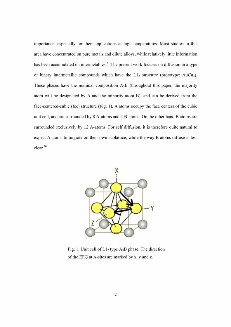
These phases have the nominal composition A3B (throughout this paper, the majority

atom will be designated by A and the minority atom B), and can be derived from the

face-centered-cubic (fcc) structure (Fig. 1). A atoms occupy the face centers of the cubic

unit cell, and are surrounded by 8 A-atoms and 4 B-atoms. On the other hand B atoms are

surrounded exclusively by 12 A-atoms. For self diffusion, it is therefore quite natural to

expect A atoms to migrate on their own sublattice, while the way B atoms diffuse is less

clear.10

Fig. 1. Unit cell of L12 type A3B phase. The direction

of the EFG at A-sites are marked by x, y and z.

3

In previous work of Collins and coworkers1, 2, 4 PAC was applied to L12 type rare

earth indides RIn3 (R=La, Ce, Pr, Nd, Gd, Er, Y) and LaSn3. All these phases appear in

binary phase diagrams as “line” compounds, which means a compound having a definite

composition, such as : 75 : 25A B = . These compounds usually have phase fields

narrower than 1 at.% and are commonly assumed to have properties independent of

composition. However it has been found that jump frequencies in some of the indide and

stanide phases mentioned above can vary significantly when measured at different phase

boundary compositions. The present work extends jump frequency measurement to

additional rare earth indides and also to rare earth gallides and aluminides in an effort to

understand the systematics of jump frequencies, including activation enthalpies.

Measurements were made for both more indium rich (designated as A) and less indium

rich (designated as B) phase boundary compositions in order to shed light on the jump

mechanism.

4

2. Theory

2.1 Perturbed angular correlation spectroscopy

Perturbed angular correlation spectroscopy is a time domain spectroscopy

technique. It measures the coincidence rate of the emission of gamma rays from the probe

nuclear decay, which gives information on the hyperfine interactions between the nuclear

moments of probe atoms and the internal magnetic field and/or electric field gradient at

the probe atom sites.

2.1.1 Spin alignment and unperturbed angular correlation of gamma-rays

In PAC spectroscopy, radioactive nuclides which emit two consecutive gamma-rays

during their decay process are used as probes. The gamma rays are detected by two or

more detectors and the coincidence rate is recorded as a function of time. Between the

emissions of the two gamma-rays, the nuclides stay at on an intermediate energy level.

The detection of the first gamma-ray amounts to a selection of preferred nuclear spin

substates of the intermediate level, or in other words, a spin alignment with respect to the

direction of the first gamma-ray is produced.5 As a result the angular distribution of the

second gamma-ray emission is no longer random, but correlated to the direction of the

first gamma-ray (Fig. 2). The probability of detecting the second gamma-ray at an angle θ

with respect to the first one is described by the angular correlation function

( ) 1 (cos ),k kk even

W A Pθ θ

= + ∑ (2.1)

5

in which Pk’s are even order Legendre polynomials and Ak’s describe the degree of

anisotropy and are functions of the spin quantum numbers of the initial, intermediate and

final levels of the decay.

γ2

Stop dectector

Start dectector

γ1

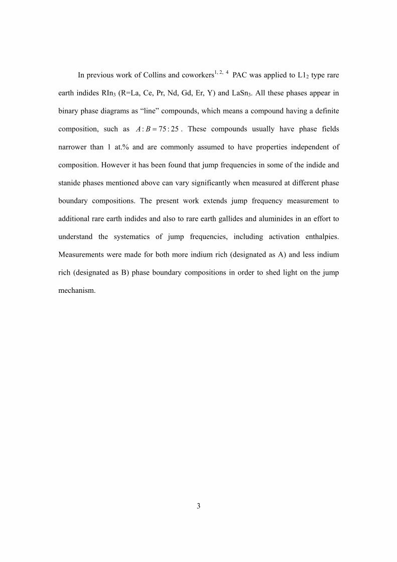
Fig. 2. Angular correlation of two gamma-ray emissions.

2.1.2 Spin precession and perturbed angular correlation of gamma-rays

An magnetic field or electric field gradient present at the site of the probe nuclei

will cause hyperfine splitting of the energy level of the intermediate state. As a result the

populations of the nuclear spin substates evolve with time and W(θ) becomes

time-dependent. This is analogous to classical spin precession in an external field. For a

random distribution of internal field orientations, Eq.(2.1) becomes5

( , ) 1 ( ) (cos ).k k kk even

W t A G t Pθ θ

= + ∑ (2.2)

Gk(t) is called the perturbation function and its detailed form depends on the type of

hyperfine interaction in question and the spin quantum numbers of the initial,

6

intermediate and final states of the decay.

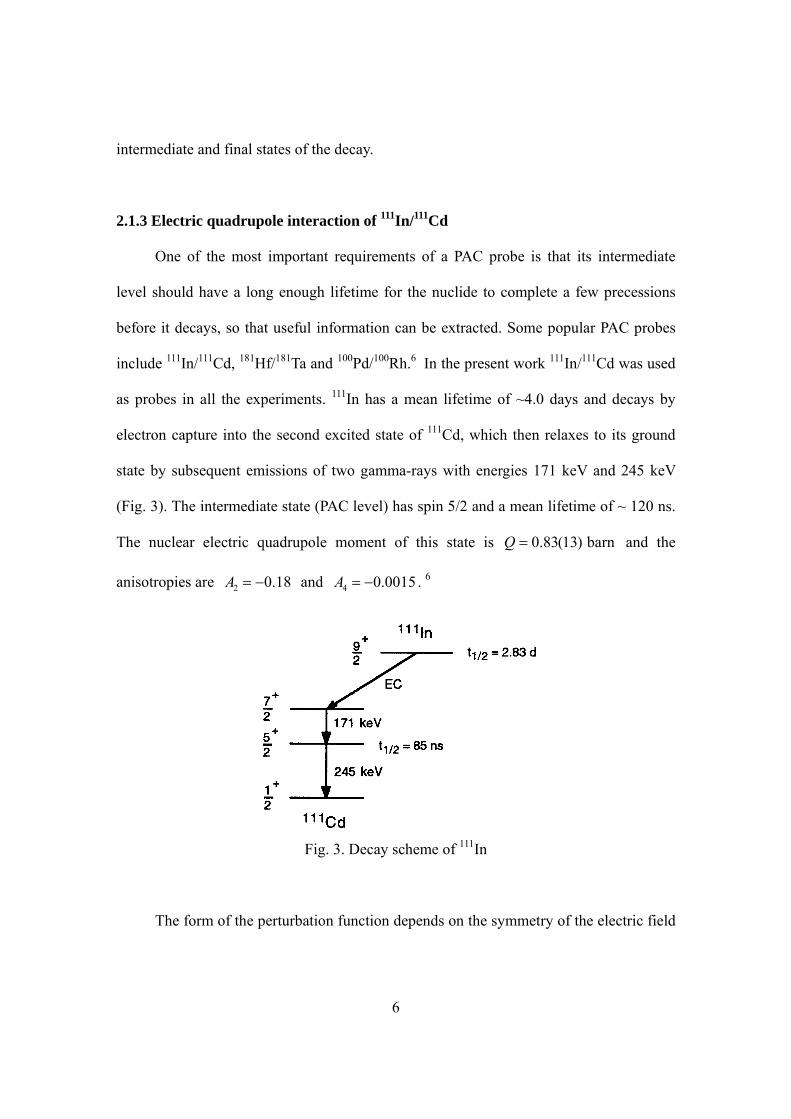
2.1.3 Electric quadrupole interaction of 111In/111Cd

One of the most important requirements of a PAC probe is that its intermediate

level should have a long enough lifetime for the nuclide to complete a few precessions

before it decays, so that useful information can be extracted. Some popular PAC probes

include 111In/111Cd, 181Hf/181Ta and 100Pd/100Rh.6 In the present work 111In/111Cd was used

as probes in all the experiments. 111In has a mean lifetime of ~4.0 days and decays by

electron capture into the second excited state of 111Cd, which then relaxes to its ground

state by subsequent emissions of two gamma-rays with energies 171 keV and 245 keV

(Fig. 3). The intermediate state (PAC level) has spin 5/2 and a mean lifetime of ~ 120 ns.

The nuclear electric quadrupole moment of this state is 0.83(13) barnQ = and the

anisotropies are 2 0.18A = − and 4 0.0015A = − . 6

Fig. 3. Decay scheme of 111In

The form of the perturbation function depends on the symmetry of the electric field

7

gradient tensor. The EFG is a second-order tensor whose nine components are the second

derivatives of the electric potential V(r). When diagonalized by choosing a proper

coordinate system the EFG can be fully described by three diagonal elements Vxx, Vyy,

and Vzz with the convention zz yy xxV V V≥ ≥ . With the Poisson equation

0zz yy xxV V V+ + = , the EFG can be further reduced to two elements, namely zzV and η ,

where η is the EFG asymmetry parameter, defined by:

( ) / .xx yy zzV V Vη = − (2.3)

Note that by definition 0 1η≤ ≤ . It can be shown that for a site having a three-fold or

higher axis of symmetry, 0η = . The magnitude of Vij can be estimated using a simple

point charge model:

2

5lattice ions

( )(3 )(1 ) ,i j ij

ij

q x x rV

rδ

γ ∞

−= − ∑

r (2.4)

in which the summation gives the contribution from lattice ions and the factor γ ∞

accounts for the polarization of the probe atoms’ inner-shell electrons due to an external

EFG. The term (1 )γ ∞− is of order -10 to -100 and thus determines the magnitude of the

EFG.6

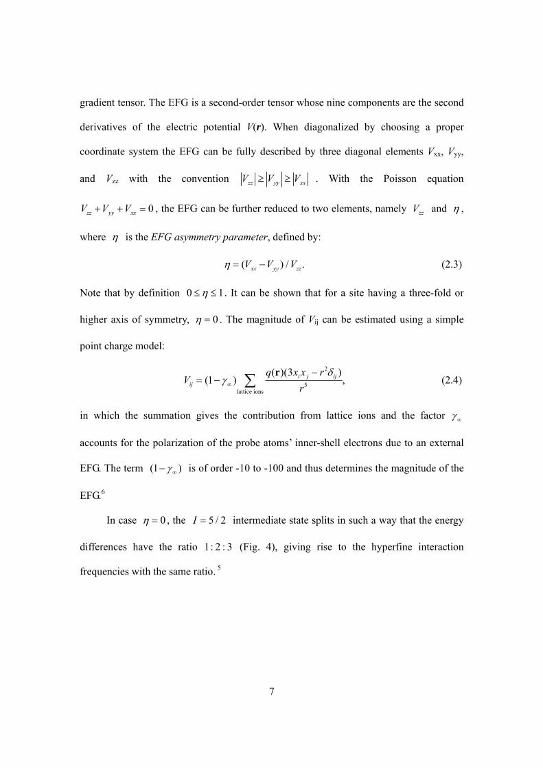
In case 0η = , the 5 / 2I = intermediate state splits in such a way that the energy

differences have the ratio 1: 2 : 3 (Fig. 4), giving rise to the hyperfine interaction

frequencies with the same ratio. 5

8

Fig. 4. Energy splitting of the 5 / 2I = intermediate state.

Moreover, for axially symmetric case ( 0η = ) in a random polycrystalline sample, the

perturbation function can be shown to have the following form:

21( ) [7 13cos(6 ) 10cos(12 ) 5cos(18 )],35

staticQ Q QG t t t tω ω ω= + + + (2.5)

in which Qω is the quadrupole interaction frequency. For half odd integer spin Qω is

defined by5

6 / 4 (2 1)Q zzeQV I Iω = −

The 2( )G t function here is labeled “static” so as to be distinguished from the dynamic

perturbation function to be introduced in the next section. 2 ( 0)G t = is always equal to 1.

And for lattice sites with cubic symmetry the perturbation function is time independent:

2 ( ) 1G t = , since no torque is exerted on the quadrupole moment. Finally if 111In/Cd

probes occupy more than one sublattice, the resultant 2 ( )G t function will be a

superposition of the 2 ( )G t functions for the individual sublattices, weighed by the

fractions of probes staying on each sublattice.

9

2.1.4 Dynamic perturbation function and the XYZ model

The rare earth indides, gallides and aluminides studied in this work have the L12

structure, shown in Fig. 1. 111In/111Cd probes naturally occupy the A-sublattice in the

indides. In the gallides and aluminides the probe atoms were made to mostly occupy also

the A-sublattice by making the sample deficient in A elements (see section 3.3). At

A-sites the EFG is axially symmetric and perpendicular to the faces of the unit cell. Thus

there are three orthogonal EFG directions, labeled as X, Y and Z in Fig. 1. The jump of a

probe atom to a nearest neighbor site always results in reorientation of the EFG by 90º.

Thus the probe experiences a fluctuating EFG instead of a steady one as it jumps. This

leads to damping of the PAC spectrum and can be described by introducing a parameter λ

into the 2 ( )G t function:

2 2( ) ( )t staticG t e G tλ−= (2.6)

Winkler and Gerdau7 first studied such a situation and developed a model later called the

XYZ model8. Baudry and Boyer9 obtained an empirical relation between λ and the mean

frequency at which the EFG changes to a single other orientation for a given probe

( EFGw ). Approximate expressions of λ were found for the slow fluctuation regime

( EFG Qw ω ) and the fast fluctuation regime ( 20EFG Qw ω ) respectively:

( 1) in slow fluctuation regimeEFGN wλ − (2.7)

and

2100( / 6) (1 / ) in fast fluctuation regime,Q EFGNwλ ω (2.8)

where N is the number of different orientations of the EFG. No analytic expression can be

10

given for the intermediate regime ( 20Q EFG Qwω ω< < ), where maximum damping occurs.

The jump frequency of a probe atom w is equal to the product of the frequency at which

the EFG changes to a specific orientation and number of different EFG orientations that a

probe can jump to, other than its original one. Therefore ( 1) EFGw N w= − , so that for the

slow fluctuation regime we have the simple relation w λ= .

2.1.5 Inhomogeneous broadening

Defects in samples cause distortion to the EFG, the degree of which differs for different

probe atoms depending on their distance to the defect. This causes inhomogeneous

broadening of the PAC spectrum, which can be described by

1 32 2

21( ) [7 13cos(6 )e 10cos(12 )e 5cos(18 )e ],35

t tstatic tQ Q QG t t t t

σ σσω ω ω− −−= + + + (2.9)

where σ is a parameter that describes the degree of inhomogeneous broadening. σ

was found to be less than ~ 1 Mrad/s in all the samples studied in the present work. When

fitting the spectrum, it is difficult to separate the damping caused by inhomogeneous

broadening from that caused by dynamic broadening, and thus only one parameter,

namely λ , was used in the fitting to describe the damping. Therefore the fitted value of

λ may be slightly higher than its true value. This effect can be ignored when λ is large,

but may be important at low temperature.

2.2 Diffusion mechanisms and point defects in L12 phases

11

This section will briefly discuss possible diffusion mechanisms feasible in A3B

compounds of L12 type. We are mainly concerned with the majority constituent diffusion,

since probe atoms mostly occupy the A-sublattice.

(1) The most elementary diffusion mechanism is an A-monovacancy mechanism.

Probe atoms can diffuse as a consequence of random walks of A-vacancies (VA) on their

own sublattice. The jump frequency of probe atoms is proportional to the concentration of

A-vacancies [VA], the number of near neighbor A sites z and the rate of exchange between

an A-vacancy and a neighboring probe atom w2:

2[ ]Aw z V w= (2.10)

For this mechanism, the probe jump frequency can be related to the macroscopic quantity

diffusivity D by10

216

D fd w= (2.11)

where d is the jump length (1 / 2 of lattice parameter) and f is the correlation factor,

which is between 1 and 0 and accounts for the nonrandomness of direction selection

when a probe atom jumps. For vacancy self-diffusion on the A-sublattice f is equal to

0.68911, and for impurity diffusion it is a function of temperature and can be calculated

using the five frequency model12.

(2) A similar mechanism is the divacancy mechanism. Two monovacancies VA and

VB can combine to form a divacancy due to energy advantage. The two members of the

vacancy pair then move together but always on their own sublattice, leading to probe

migration. Generally the concentration of divacancy rises faster than that of

monovacancy10 and is thus more important at high temperature. However the long

12

distance jump required of VB in the L12 structure makes the migration of divacancies

difficult to happen.

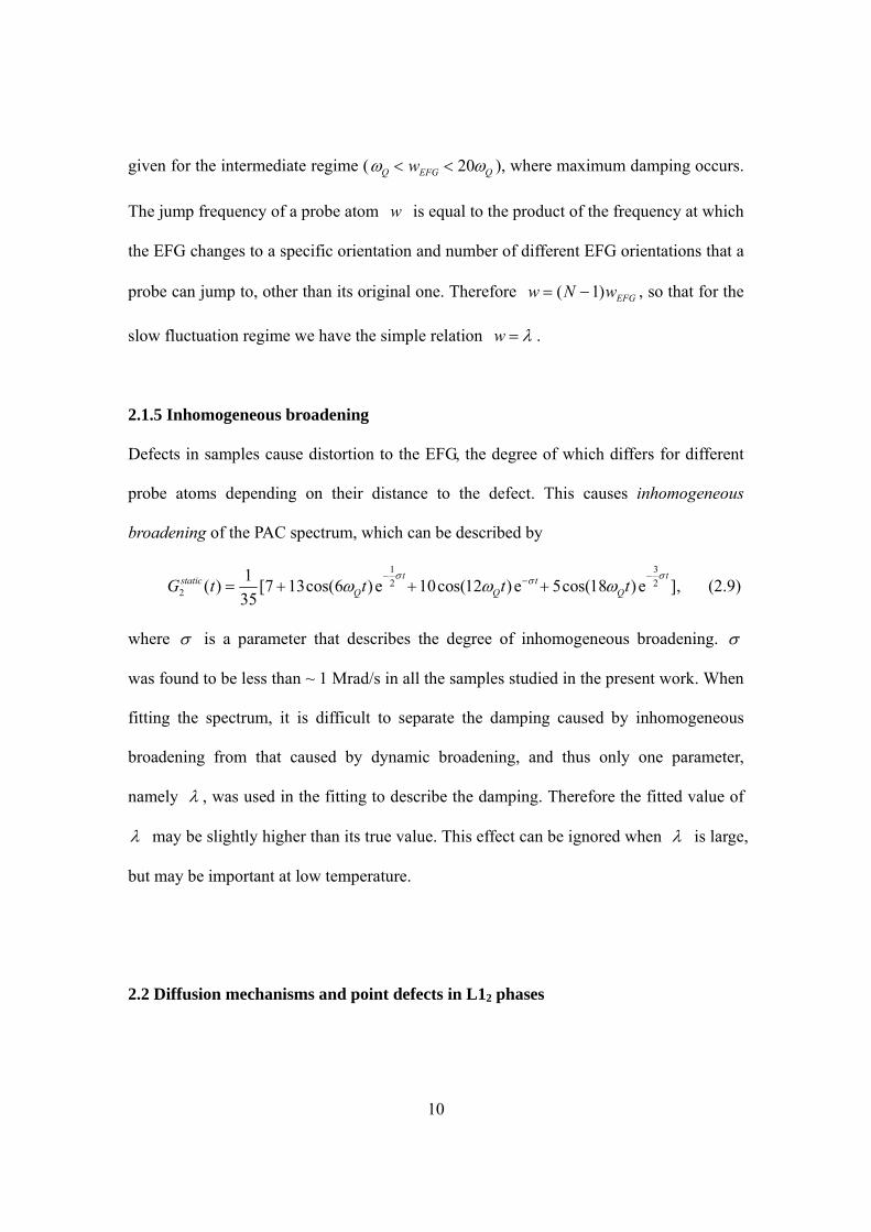
(3) A six jump cycle mechanism12 could also lead to 111Cd probe migration. Fig. 5

shows an example of a B-vacancy six jump circle. Here a B-vacancy makes six

consecutive jumps to near neighbor sites, resulting in the exchange of two B atoms and

the exchange of the vacancy and an A atom. Similarly an A-vacancy six jump circle leads

to exchange of two B atoms and migration of the A-vacancy.

1,52,6

34

Fig. 5. Scheme of B-vacancy six jump cycle mechanism

(4) In a vacancy conversion mechanism, point defects may react with each other to

form new types of point defects, if such a reaction can lead to lower total free energy. The

reaction that concerns us here is V + In VB A B AA→ + , in which B-vacancies are

converted into A-vacancies and thus contribute to the diffusion on the A-sublattice

through the A-monovacancy mechanism.

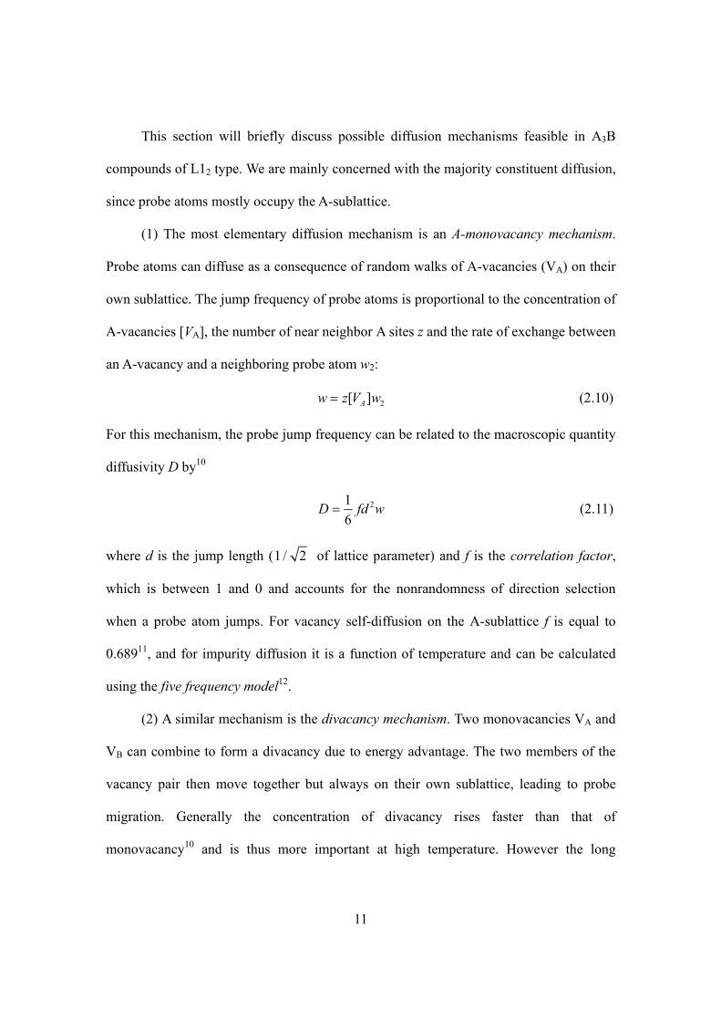
(5) Zener13 proposed the ring exchange mechanism for bcc and fcc metals, in

which two or more atoms jump simultaneously on a ring to their near neighbor sites. It is

13

possible to think of 2-ring, 3-ring or 4-ring diffusion (Fig. 6) in fcc metals. The exchange

mechanism is usually dismissed as an unrealistic picture since direct exchange of

neighboring atoms in a close-packed crystal would cause great distortion of the lattice

and require considerable amount of energy.10 Zener showed in his early calculation for Cu

metal that 3-ring and 4-ring diffusion are much less energetically costly per atom than

2-ring diffusion (the direct exchange of two atoms) and thus might be a feasible

mechanism in the fcc structure, with the 4-ring mechanism requiring the lowest energy of

all. 13

Fig. 6. Scheme of 3-ring and 4-ring diffusion in fcc metals (taken from Ref.13)

Except for the ring exchange mechanism, all the other mechanisms mentioned

above are vacancy-mediated, which justifies a short discussion of point defects in solids.

At least four types of point defects can form in ordered binary intermetallics, namely

vacancies defects VA and VB, and anti-site defects BA and AB. The most likely defect to

form in L12 crystals is probably a five-defect:

0 4 ,A AV B→ + (2.12)

with equilibrium constant

45 5[ ] [ ] exp( / ),A B BK V A G k T= = − (2.13)

14

in which [ ]AV is the mole fraction of vacancies on the A-sublattice, etc. At stoichiometry,

3[ ] [ ]4B AA V= , so that one has

1/50 5[ ] exp( / ) (3 / 4) exp( / 5 ),eff

A F B BV C G k T G k T≡ − = − (2.14)

where 0C is a constant and effFG is the effective free energy of formation of an

A-vacancy.

At nonstoichiometry, structural defects arise to compensate for the deviation form

stoichiometry. These defects could be the dominant type of defects when the compound is

sufficiently off-stoichiometry and when temperature is not too high. It can be shown by

thermodynamic consideration that [VB] and [AB] increase monotonically, and [VA] and

[BA] decrease monotonically as the compound becomes more A-rich.14

15

3. Experimental methods

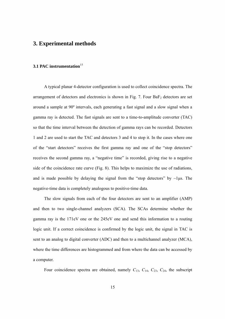
3.1 PAC instrumentation15

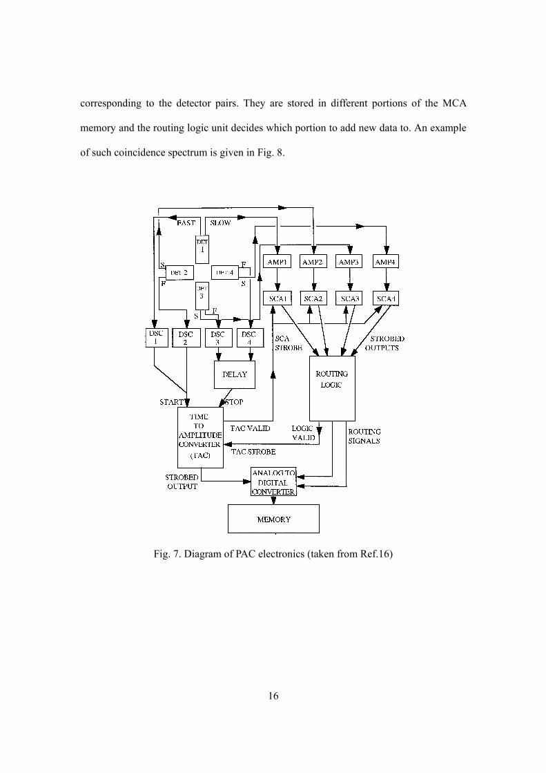
A typical planar 4-detector configuration is used to collect coincidence spectra. The

arrangement of detectors and electronics is shown in Fig. 7. Four BaF2 detectors are set

around a sample at 90º intervals, each generating a fast signal and a slow signal when a

gamma ray is detected. The fast signals are sent to a time-to-amplitude converter (TAC)

so that the time interval between the detection of gamma rays can be recorded. Detectors

1 and 2 are used to start the TAC and detectors 3 and 4 to stop it. In the cases where one

of the “start detectors” receives the first gamma ray and one of the “stop detectors”

receives the second gamma ray, a “negative time” is recorded, giving rise to a negative

side of the coincidence rate curve (Fig. 8). This helps to maximize the use of radiations,

and is made possible by delaying the signal from the “stop detectors” by ~1μs. The

negative-time data is completely analogous to positive-time data.

The slow signals from each of the four detectors are sent to an amplifier (AMP)

and then to two single-channel analyzers (SCA). The SCAs determine whether the

gamma ray is the 171eV one or the 245eV one and send this information to a routing

logic unit. If a correct coincidence is confirmed by the logic unit, the signal in TAC is

sent to an analog to digital converter (ADC) and then to a multichannel analyzer (MCA),

where the time differences are histogrammed and from where the data can be accessed by

a computer.

Four coincidence spectra are obtained, namely C13, C14, C23, C24, the subscript

16

corresponding to the detector pairs. They are stored in different portions of the MCA

memory and the routing logic unit decides which portion to add new data to. An example

of such coincidence spectrum is given in Fig. 8.

Fig. 7. Diagram of PAC electronics (taken from Ref.16)

17

-400 400

Coi

ncid

ence

rate

Time (ns)0

Fig. 8. Coincidence rate curve of 111In/Cd in ferromagnetic iron

for two detectors at 180º

3.2 Data reduction17

For actual experiments, Eq.(2.2) is modified by an angular attenuation factor aγ

which accounts for the solid angles that the detectors subtend to the sample:

2 2 2( , ) 1 ( ) (cos ).aW t A G t Pθ γ θ= + (3.1)

aγ was about 0.7 in our experiments. (The 4 4( )A G t term is omitted as it is not detected

for the 4-detector configuration mentioned above.) The coincidence rate curve shown in

Fig. 8 can be described by

/( , ) ( , ) ( , ) ,tij ij ij ij ijC t C t B N e W t Bτθ θ θ−= + = + (3.2)

18

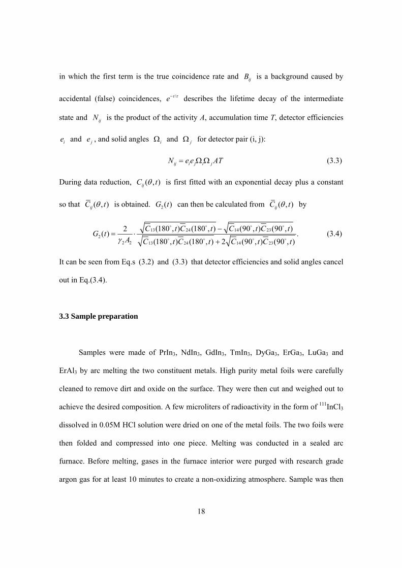
in which the first term is the true coincidence rate and ijB is a background caused by

accidental (false) coincidences, /te τ− describes the lifetime decay of the intermediate

state and ijN is the product of the activity A, accumulation time T, detector efficiencies

ie and je , and solid angles iΩ and jΩ for detector pair (i, j):

ij i j i jN e e AT= Ω Ω (3.3)

During data reduction, ( , )ijC tθ is first fitted with an exponential decay plus a constant

so that ( , )ijC tθ is obtained. 2 ( )G t can then be calculated from ( , )ijC tθ by

13 24 14 232

2 2 13 24 14 23

(180 , ) (180 , ) (90 , ) (90 , )2( ) .(180 , ) (180 , ) 2 (90 , ) (90 , )

C t C t C t C tG tA C t C t C t C tγ

−= ⋅

+ (3.4)

It can be seen from Eq.s (3.2) and (3.3) that detector efficiencies and solid angles cancel

out in Eq.(3.4).

3.3 Sample preparation

Samples were made of PrIn3, NdIn3, GdIn3, TmIn3, DyGa3, ErGa3, LuGa3 and

ErAl3 by arc melting the two constituent metals. High purity metal foils were carefully

cleaned to remove dirt and oxide on the surface. They were then cut and weighed out to

achieve the desired composition. A few microliters of radioactivity in the form of 111InCl3

dissolved in 0.05M HCl solution were dried on one of the metal foils. The two foils were

then folded and compressed into one piece. Melting was conducted in a sealed arc

furnace. Before melting, gases in the furnace interior were purged with research grade

argon gas for at least 10 minutes to create a non-oxidizing atmosphere. Sample was then

19

melted by passing through it a DC current of 45A or 55A for ~1sec, depending on the

melting point of the metals involved. Sample was then turned over and melted once more

for ~1sec. The thus obtained sample was usually in a spherical shape, indicating that the

two constituent metals had fully mixed.

Each sample was weighed again after the melting and the mass loss was calculated.

The composition range of the sample was then calculated by assuming the mass loss was

entirely due to loss of one constituent or the other. The masses of the samples were

between 40 mg to 80 mg and mass losses were between 1mg to 4 mg. Compared with arc

melting of many rare earth-aluminum alloys, in which mass losses were usually less than

1 mg, the relatively large mass losses in gallide and indide samples were most likely

caused by evaporation of gallium and indium during melt, as these two elements have

high vapor pressures.

A3B samples were prepared to have either A-rich or A-poor mean compositions,

usually a few percent away from the stoichiometry. So the actual samples were a mixture

of the desired A3B phase and a small amount of its adjacent phases.

20

3.4 Measurement at high temperature

Spectra were collected from RT to 1200 K. High temperature measurement was

carried out in a high vacuum (~10-8 mBar) chamber. The sample was heated by three

tungsten filaments about 1 cm away from it and was in touch with a K-type or R-type

thermocouple which was used to measure and control the temperature. The high

temperature and high vacuum environment could lead to significant In or Ga evaporation

for some samples and could give rise to two problems: 1, The sample tends to lose In or

Ga over time and its composition changes. 2, 111In/Cd probes that diffuse into the wall of

the vacuum chamber can produce an artificial cubic signal. In order to reduce evaporation,

samples were wrapped in 0.001 inch thick iron foil. Iron was chosen because indium is

insoluble in it and indium and iron liquids are immiscible. Coincidence spectra were

collected for ~24 hours per measurement for most samples, and for ~ 8 hours per

measurement for samples which tend to have significant In outdiffusion.

21

4. Results

4.1 PrIn3

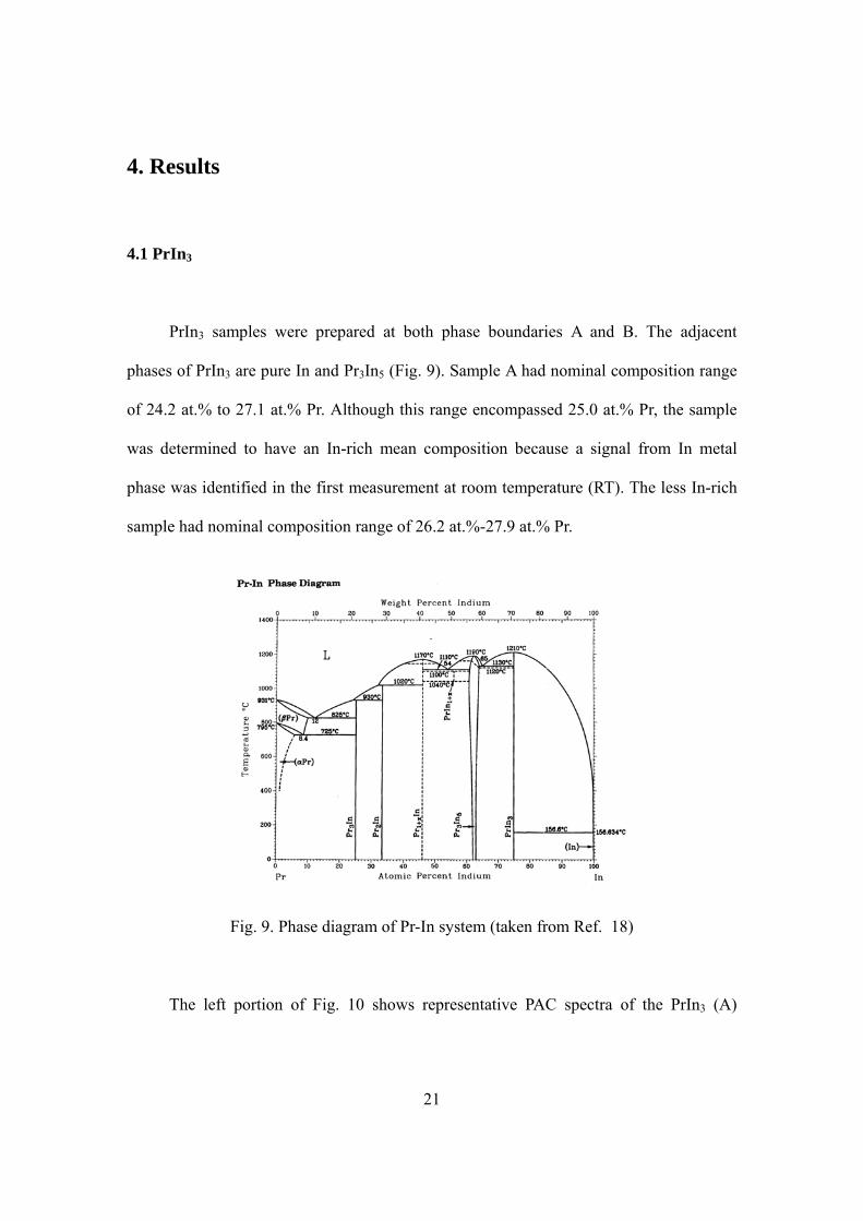
PrIn3 samples were prepared at both phase boundaries A and B. The adjacent

phases of PrIn3 are pure In and Pr3In5 (Fig. 9). Sample A had nominal composition range

of 24.2 at.% to 27.1 at.% Pr. Although this range encompassed 25.0 at.% Pr, the sample

was determined to have an In-rich mean composition because a signal from In metal

phase was identified in the first measurement at room temperature (RT). The less In-rich

sample had nominal composition range of 26.2 at.%-27.9 at.% Pr.

Fig. 9. Phase diagram of Pr-In system (taken from Ref. 18)

The left portion of Fig. 10 shows representative PAC spectra of the PrIn3 (A)

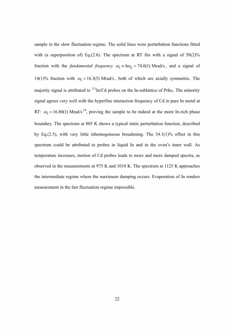
22

sample in the slow fluctuation regime. The solid lines were perturbation functions fitted

with (a superposition of) Eq.(2.6). The spectrum at RT fits with a signal of 58(2)%

fraction with the fundamental frequency 0 6 74.0(1) Mrad/sQω ω≡ = , and a signal of

14(1)% fraction with 0 16.3(5) Mrad/sω = , both of which are axially symmetric. The

majority signal is attributed to 111In/Cd probes on the In-sublattice of PrIn3. The minority

signal agrees very well with the hyperfine interaction frequency of Cd in pure In metal at

RT: 0 16.80(1) Mrad/sω = 19, proving the sample to be indeed at the more In-rich phase

boundary. The spectrum at 805 K shows a typical static perturbation function, described

by Eq.(2.5), with very little inhomogeneous broadening. The 34.1(1)% offset in this

spectrum could be attributed to probes in liquid In and in the oven’s inner wall. As

temperature increases, motion of Cd probes leads to more and more damped spectra, as

observed in the measurements at 975 K and 1018 K. The spectrum at 1125 K approaches

the intermediate regime where the maximum damping occurs. Evaporation of In renders

measurement in the fast fluctuation regime impossible.

23

Fig. 10. PAC spectra of PrIn3 at phase boundary compositions A and B. Solid lines

are best fits of perturbation functions. The arrow indicates a signal from the

adjacent Pr3In5 phase.

0.00

0.25

0.50

0.75

1.00

1.25

0.00

0.25

0.50

0.75

1.00

0.00

0.25

0.50

0.75

1.00

0.25

0.50

0.75

1.00

1.25

0.25

0.50

0.75

1.00

1.25

0.25

0.50

0.75

1.00

1.25

1.50

0.00

0.25

0.50

0.75

1.00

400 300 200 100 0 -100 -200 -300 -4000.00

0.25

0.50

0.75

1.00

400 300 200 100 0 -100 -200 -300 -4000.25

0.50

0.75

1.00

1.25

PrIn3 (A)

G2(t) 975 K

1178 K

G2(t)

1082 K

1231 K1125 K

1018 K

PrIn3 (B)

t [ns]

1018 K

RT

805 K

t [ns]

24

The spectra of PrIn3 (B) sample (Fig. 10 right) fit with two signals. The dominant

signal is identical to the high frequency signal in the sample A and is naturally attributed

to probes on the In-sublattice of PrIn3. The other signal (indicated by arrow in Fig. 10)

has a fundamental frequency 0 100.0(5) Mrad/sω = and 0.929(7)η = at 1082 K, and is

attributed to probes in the neighboring phase Pr3In5. It takes about 100 K increase in

temperature for sample B to show the same amount of damping as sample A does.

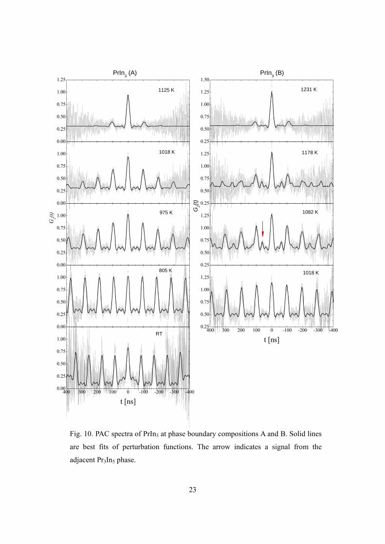
The fitted values of λ (equal to jump frequency w) are shown in Fig. 11. The

three measurements at high temperature of the B sample fall on a straight trend line. The

deviation of the two measurements at lower temperature could be explained by misfit due

to inhomogeneous broadening.

The sequence of measurement on the A sample is numbered in Fig. 11 (The first

measurement at RT is not included). The first four measurements fall on a straight trend

line. The 5th and 6th measurements fall below this trend line, opposite to what one would

expect if there was inhomogeneous broadening. The 7th approached the trend line of the B

sample, and the last three measurements fall very well on it. This could be understood by

taking into consideration the volatility of Indium. High temperature and high vacuum

condition caused In to evaporate out of the In-rich sample, turning it from the A phase

boundary to the B phase boundary, and thus moved w from one trend line toward the

other. This change of behavior and the consistency of the last three measurements of the

B sample with those of the A sample is further proof that the two samples were indeed at

the less In-rich and more In-rich phase boundaries respectively. The straight lines in Fig.

11 are jump frequencies fitted with an Arrhenius temperature dependence

0 exp( / ),w w Q kT= − (4.1)

25

in which 0w is a prefactor and Q is the activation enthalpy for Cd probes to jump. Points

1-4 were used in the fitting for the A boundary. Points 8-10 together with the three

triangle points at high temperature were used in the fitting for the B phase boundary. The

best fit values of 0w and Q are listed in Table 1.

9.0 9.5 10.0 10.5 11.0 11.5 12.0 12.5 13.0 13.5 14.0 14.5 15.0105

106

107

1250 1200 1150 1100 1050 1000 950 900 850 800

PrIn3 (B) PrIn3 (A)

10

9

87

6

5

4

3

1

w (H

z)

1/kBT (eV-1)

2

B

T (K)

A

Fig. 11. Arrhenius plot of Cd jump frequencies in PrIn3 at two phase boundaries and their

best fits. The numbers designate the order of measurement on the B sample.

26

4.2 NdIn3

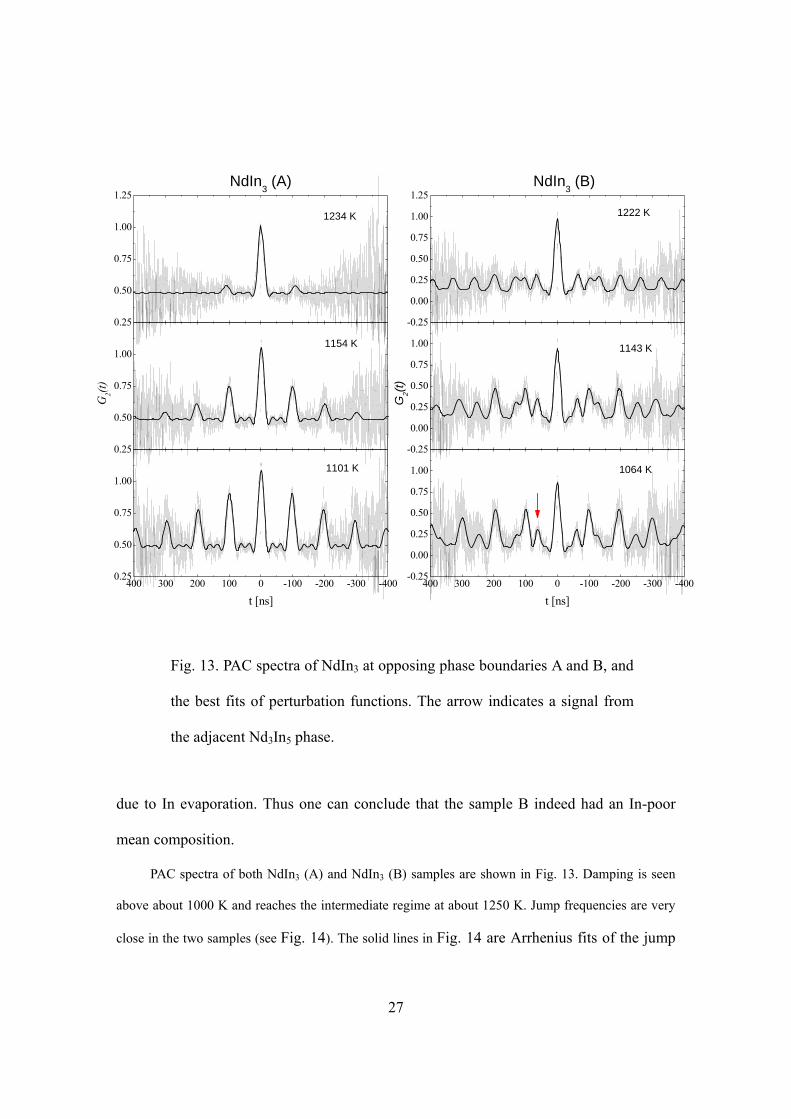
Jump frequencies were measured in NdIn3 for both phase boundaries A and B. The

sample A had nominal composition range 15.8-19.9 at.% Nd. And like in PrIn3 (A), a

signal corresponding to In metal was observed at RT ( 0 17.0(3) Mrad/sω = ), proving its

mean composition to be In-rich. The sample B (composition range 22.0-30.8 at.%.)

showed a majority signal of 0 62.95(9) Mrad/sω = and a minority signal (pointed by

arrow in Fig. 13) of 0 98.8(4) Mrad/s, 0.94(1)ω η= = at 1064 K, which is attributed to

the neighboring phase Nd3In5 for two reasons: (1) It is very similar to the minority signal

seen in PrIn3 (B). (2) The percentage of this signal increased gradually during high

temperature measurements, which could be explained by the increase of Nd3In5 fraction

Fig. 12. Phase diagram of Nd-In system (taken from Ref. 18)

27

0.25

0.50

0.75

1.00

1.25

0.25

0.50

0.75

1.00

400 300 200 100 0 -100 -200 -300 -4000.25

0.50

0.75

1.00

-0.25

0.00

0.25

0.50

0.75

1.00

400 300 200 100 0 -100 -200 -300 -400-0.25

0.00

0.25

0.50

0.75

1.00

-0.25

0.00

0.25

0.50

0.75

1.00

1.25NdIn3 (A)

G2(t)

t [ns]

1101 K

1143 K

G2(t)

1064 K

t [ns]

1222 K1234 K

1154 K

NdIn3 (B)

Fig. 13. PAC spectra of NdIn3 at opposing phase boundaries A and B, and

the best fits of perturbation functions. The arrow indicates a signal from

the adjacent Nd3In5 phase.

due to In evaporation. Thus one can conclude that the sample B indeed had an In-poor

mean composition.

PAC spectra of both NdIn3 (A) and NdIn3 (B) samples are shown in Fig. 13. Damping is seen

above about 1000 K and reaches the intermediate regime at about 1250 K. Jump frequencies are very

close in the two samples (see Fig. 14). The solid lines in Fig. 14 are Arrhenius fits of the jump

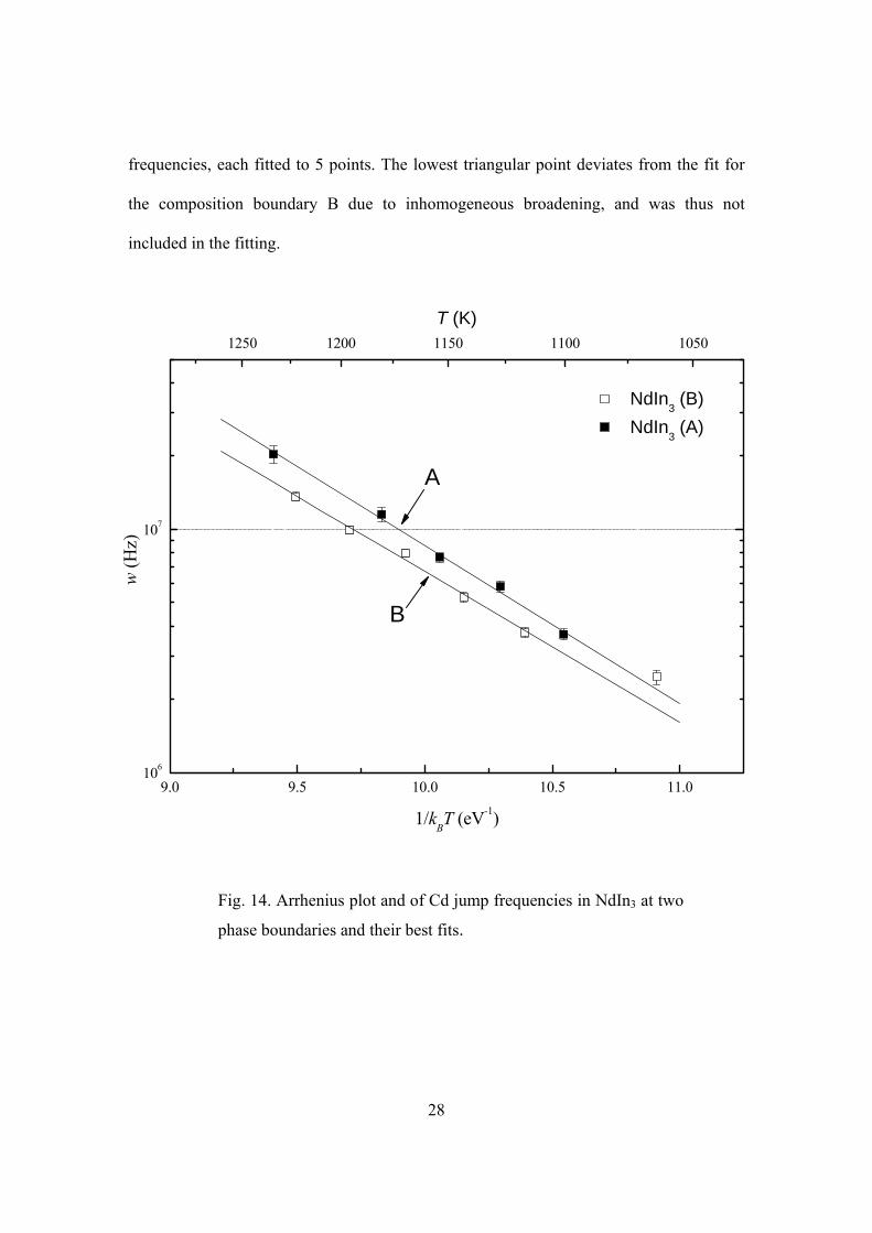
28

frequencies, each fitted to 5 points. The lowest triangular point deviates from the fit for

the composition boundary B due to inhomogeneous broadening, and was thus not

included in the fitting.

9.0 9.5 10.0 10.5 11.0106

107

1250 1200 1150 1100 1050

B

NdIn3 (B) NdIn3 (A)

w (H

z)

1/kBT (eV-1)

A

T (K)

Fig. 14. Arrhenius plot and of Cd jump frequencies in NdIn3 at two

phase boundaries and their best fits.

29

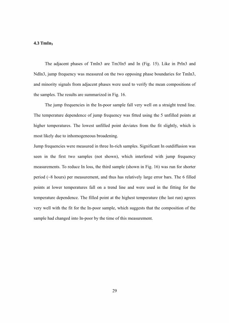
4.3 TmIn3

The adjacent phases of TmIn3 are Tm3In5 and In (Fig. 15). Like in PrIn3 and

NdIn3, jump frequency was measured on the two opposing phase boundaries for TmIn3,

and minority signals from adjacent phases were used to verify the mean compositions of

the samples. The results are summarized in Fig. 16.

The jump frequencies in the In-poor sample fall very well on a straight trend line.

The temperature dependence of jump frequency was fitted using the 5 unfilled points at

higher temperatures. The lowest unfilled point deviates from the fit slightly, which is

most likely due to inhomogeneous broadening.

Jump frequencies were measured in three In-rich samples. Significant In outdiffusion was

seen in the first two samples (not shown), which interfered with jump frequency

measurements. To reduce In loss, the third sample (shown in Fig. 16) was run for shorter

period (~8 hours) per measurement, and thus has relatively large error bars. The 6 filled

points at lower temperatures fall on a trend line and were used in the fitting for the

temperature dependence. The filled point at the highest temperature (the last run) agrees

very well with the fit for the In-poor sample, which suggests that the composition of the

sample had changed into In-poor by the time of this measurement.

30

Fig. 15. Phase diagram of Tm-In system (taken from Ref. 18)

9.6 9.8 10.0 10.2 10.4 10.6 10.8 11.0 11.2 11.4 11.6 11.8

106

107

1200 1150 1100 1050 1000

TmIn3 (B)TmIn3 (A)

w (H

z)

1/kBT (eV-1)

A

T (K)

B

Fig. 16. Arrhenius plot of Cd jump frequencies in TmIn3 at opposing phase

boundaries and their best fits.

31

4.4 GdIn3

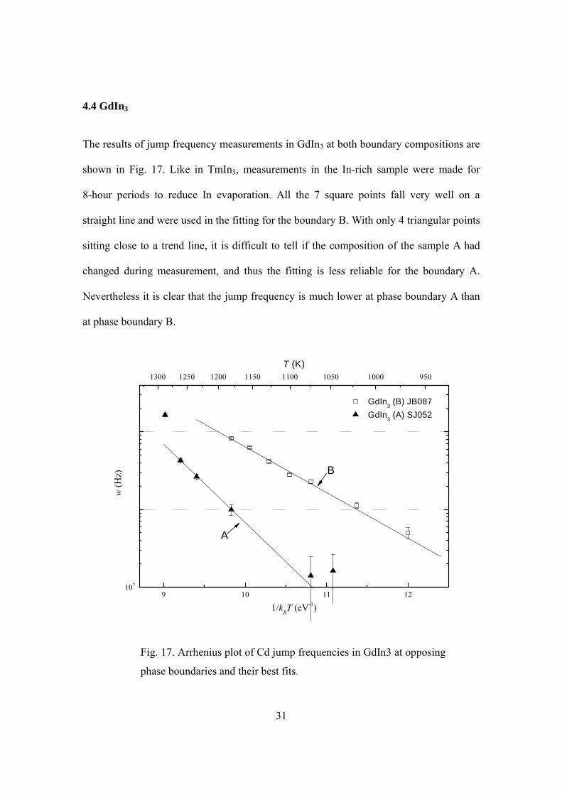
The results of jump frequency measurements in GdIn3 at both boundary compositions are

shown in Fig. 17. Like in TmIn3, measurements in the In-rich sample were made for

8-hour periods to reduce In evaporation. All the 7 square points fall very well on a

straight line and were used in the fitting for the boundary B. With only 4 triangular points

sitting close to a trend line, it is difficult to tell if the composition of the sample A had

changed during measurement, and thus the fitting is less reliable for the boundary A.

Nevertheless it is clear that the jump frequency is much lower at phase boundary A than

at phase boundary B.

9 10 11 12105

1300 1250 1200 1150 1100 1050 1000 950

GdIn3 (B) JB087 GdIn3 (A) SJ052

w (H

z)

1/kBT (eV-1)

B

T (K)

A

Fig. 17. Arrhenius plot of Cd jump frequencies in GdIn3 at opposing

phase boundaries and their best fits.

32

4.5 DyGa3, ErGa3, LuGa3 and ErAl3

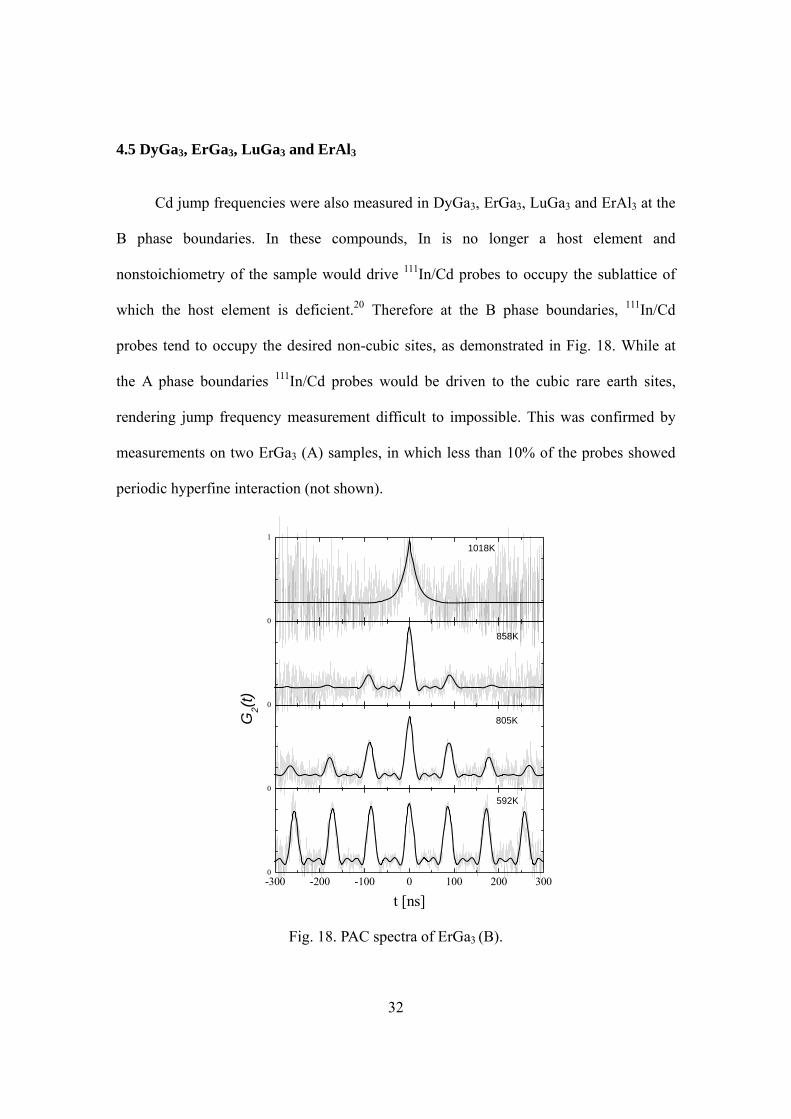
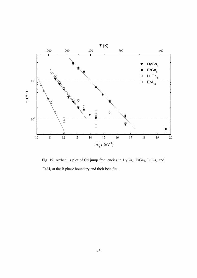
Cd jump frequencies were also measured in DyGa3, ErGa3, LuGa3 and ErAl3 at the

B phase boundaries. In these compounds, In is no longer a host element and

nonstoichiometry of the sample would drive 111In/Cd probes to occupy the sublattice of

which the host element is deficient.20 Therefore at the B phase boundaries, 111In/Cd

probes tend to occupy the desired non-cubic sites, as demonstrated in Fig. 18. While at

the A phase boundaries 111In/Cd probes would be driven to the cubic rare earth sites,

rendering jump frequency measurement difficult to impossible. This was confirmed by

measurements on two ErGa3 (A) samples, in which less than 10% of the probes showed

periodic hyperfine interaction (not shown).

0

1

0

0

-300 -200 -100 0 100 200 3000

1018K

858K

G2(t)

805K

t [ns]

592K

Fig. 18. PAC spectra of ErGa3 (B).

33

Fig. 18 shows representative PAC spectra and fitted perturbation functions of

ErGa3 (B). The three spectra at the bottom exhibited typical behavior in the slow

fluctuation regime, where damping increases with temperature. The spectrum on the top

is an example of behavior in the fast fluctuation regime, where the periodic interaction is

no longer visible and the damping decreases with temperature. Similar spectra were

obtained for DyGa3, LuGa3 and ErAl3 in the slow fluctuation regime, however damping

in these phases was seen at much higher temperature. The jump frequencies in all the four

phases and the fits to Arrhenius temperature dependence are shown in Fig. 19. Only

points that fall close to the straight lines were used in the fitting. The fitted values of Q

and 0w are listed in Table 1. Jump frequencies in all the four samples deviate from their

trend lines at low temperatures. This could be caused by inhomogeneous broadening due

to distant defects. It is also possible that there exists a second jump mechanism, which

has much lower an activation enthalpy and thus is not visible at high temperature but

becomes important at low temperature.

34

10 11 12 13 14 15 16 17 18 19 20

106

107

1000 900 800 700 600

DyGa3

ErGa3

LuGa3

ErAl3

w (H

z)

1/kBT (eV-1)

T (K)

Fig. 19. Arrhenius plot of Cd jump frequencies in DyGa3, ErGa3, LuGa3 and

ErAl3 at the B phase boundary and their best fits.

35

5. Discussion

5.1 Cd jump frequencies in various L12 intermetallics

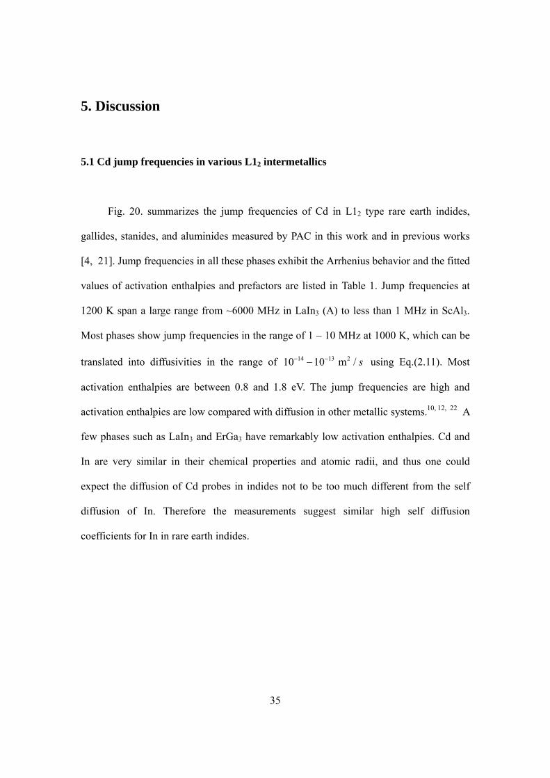
Fig. 20. summarizes the jump frequencies of Cd in L12 type rare earth indides,

gallides, stanides, and aluminides measured by PAC in this work and in previous works

[4, 21]. Jump frequencies in all these phases exhibit the Arrhenius behavior and the fitted

values of activation enthalpies and prefactors are listed in Table 1. Jump frequencies at

1200 K span a large range from ~6000 MHz in LaIn3 (A) to less than 1 MHz in ScAl3.

Most phases show jump frequencies in the range of 1 – 10 MHz at 1000 K, which can be

translated into diffusivities in the range of 14 13 210 10 m / s− −− using Eq.(2.11). Most

activation enthalpies are between 0.8 and 1.8 eV. The jump frequencies are high and

activation enthalpies are low compared with diffusion in other metallic systems.10, 12, 22 A

few phases such as LaIn3 and ErGa3 have remarkably low activation enthalpies. Cd and

In are very similar in their chemical properties and atomic radii, and thus one could

expect the diffusion of Cd probes in indides not to be too much different from the self

diffusion of In. Therefore the measurements suggest similar high self diffusion

coefficients for In in rare earth indides.

36

Fig. 20. Cd jump frequencies in L12 intermetallics

Fig.

20.

Cd

jum

p fr

eque

ncie

s in

vario

us L

12 in

term

etal

lics m

easu

red

by P

AC

37

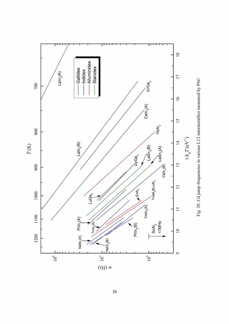
Phases

Q [eV]

w0 [THz]

Lattice Parameter23

[Å]

Source of

Data

DyGa3 (B) 1.04(9) 1.6(1.7) 4.271 This work

ErGa3 (B) 0.86(5) 1.7(1.3) 4.206 This work

LuGa3 (B) 1.10(6) 3.5(2.5) 4.180 This work

ErAl3 (B) 1.6(2) 106(208) 4.215 This work

TmAl3 1.6(1) 100(+100,-50) 4.200 [19]

LuAl3 1.6(1) 100(+100,-50) 4.187 [19]

YbAl3 1.2(1) 27(+17,-11) 4.202 [19]

LaSn3 (A) 1.22(5) 7(+5,-3) 4.769 [4]

LaSn3 (B) 1.2(1) 8(+21,-6) [4]

LaIn3 (A) 0.535(2) 1.02(0.05) 4.732 [4]

LaIn3 (B) 0.81(1) 1.4(0.2) [4]

CeIn3 (A) 0.91(4) 1.7(+1.2,-0.7) 4.691 [4]

CeIn3 (B) 1.30(7) 11(+13,-6) [4]

PrIn3 (A) 1.17(3) 3.5(1.3) 4.671 This work

PrIn3 (B) 1.75(9) 240(120) This work

NdIn3 (A) 1.50(9) 27(25) 4.653 This work

NdIn3 (B) 1.4(1) 10(10) This work

GdIn3 (A) ~2.3 ~8000 4.607 This work

GdIn3 (B) 1.36(1) 5.2(4.5) This work

ErIn3 (B) 1.13(4) 0.77(0.33) 4.564 This work

TmIn3 (A) 1.4(2) 5(8) 4.548 This work

TmIn3 (B) 1.2(1) 1.5(1.5) This work

YIn3 1.43(5) 34(+26,-15) 4.592 [4]

Table 1. Prefactors and activation enthalpies for Cd jump in

various L12 phases. Composition is unknown if not listed.

38

The most striking observation is the great composition dependence of jump

frequencies in some so called “line compounds”. For example, in LaIn3, CeIn3 and PrIn3,

jump frequencies differ by one to two orders of magnitude at the opposing phase

boundaries. In addition, reversal of behavior is observed between the early and late rare

earth indides: activation enthalpy is lower at the A phase boundary in LaIn3, CeIn3 and

PrIn3, about the same at both the boundaries in NdIn3, and higher at the A boundary in

GdIn3 and TmIn3 (see Fig. 21). The activation enthalpies in the three early rare earth

indides appear to decrease smoothly with their lattice parameters, but the late rare earth

indides do not continue this trend. These differences between the early and late rare earth

indides strongly suggest that different diffusion mechanisms are operational in the two

sets of phases.

Some late rare earth elements like Er, Tm, Lu and Yb are chemically alike and thus

one would expect to see similar diffusional behavior in their compounds. The aluminides

of the first three of these elements exhibit almost identical jump frequencies in the

temperature range investigated, while YbAl3 has jump frequencies larger by an order of

magnitude. This may suggest that YbAl3 has a much wider phase field than the other

three phases, providing more structural defects to facilitate Cd migration.

39

4.75 4.70 4.65 4.60 4.550.0

0.5

1.0

1.5

2.0

2.5

Er TmPr GdNdCe

Act

ivat

ion

enth

alpy

(eV

)

Lattice Parameter (Anstrom)

Phase boundary A Phase boundary B ?

La

Fig. 21 Activation enthalpies of Cd jump in RIn3 systems vs. lattice

parameters. (The point with ? may be subject to systematic error.)

5.2 Actual compositions of the A and B phase boundaries

Although rare earth indide samples were made to have either In-rich (A) or In-poor

(B) mean compositions, and were proven to be so by identifying signals from adjacent

phases, the actual compositions of the RIn3 phases do not necessarily have to be

absolutely In-rich or In-poor accordingly, but depends on the shapes and relative

positions of the free energy curves of the RIn3 phase and its adjacent phases. Phase field

boundaries are determined by the common tangents of the free energy curves of the phase

in question and its neighboring phases (illustrated in Fig. 22). If the free energy curve of a

40

phase is sharp and has its minimum close to that of its next phase, then the phase

boundary will be very close to stoichiometry; On the other hand if the free energy curve

is less sharp and its minimum differs much from that of its next phase, then the phase

boundary tends to be off stoichiometry. No ready information is available about the free

energy curves of the rare earth - indium systems presently studied. However it is possible

to make a rough estimation of the relative positions of the minima of these curves using

the melting points of neighboring phases. The free energy of formation of a phase is

f f fG H T SΔ = Δ − Δ , where fHΔ and fSΔ are the enthalpy and entropy of formation.

If one ignores the difference in fSΔ , then fGΔ could be roughly measured by the heat

of formation (equal to fHΔ ) , which is decided largely by the melting point of the phase,

if one further ignores the differences in the latent heat and the specific heat.

50 60 70 80 90 100B A

In

RIn3

At.% In

Mol

ar G

ibbs

ene

rgy

R3In5

Phase field of RIn3

Fig. 22. Determination of phase boundaries of RIn3 using free energy curves.

41

The phase diagrams of Pr-In, Nd-In and Tm-In are shown in Fig. 9, Fig. 12 and Fig.

15. The phase diagrams of La-In, Ce-In, Gd-In and La-Sn are not shown but are very

similar to those shown in that all the A3B phases are adjacent to a high melting point

phase A5B3 (A2B in the case of Ce-In) and a phase with very low melting point (In or Sn),

with the melting point of A3B being very close to that of A5B3. Therefore, by the rough

estimation developed above, we would expect the free energy curves of A3B and A5B3 to

have close minima while the minimum of the pure B phase is well above the other two, as

is depicted in Fig. 22. It then follows that the phase boundary B is very close to

stoichiometry (may be slightly A-rich or A-poor) and the phase boundary A is indeed on

the A-rich side and relatively far away from stoichiometry.

5.3 Diffusion mechanisms

As was suggested above, different diffusion mechanisms may prevail in the early

and late rare earth indides. The most natural (and widely accepted) mechanism for the

diffusion of the majority element would be the A-monovacancy mechanism, in which the

111In/Cd probe jumps on its own sublattice by fast passage of A-vacancies. In this

mechanism, the jump frequency of Cd would be proportional to [VA], which itself

increases monotonically as the composition of the sample moves from the phase

boundary A to B. Therefore this mechanism is consistent with the observations in GdIn3,

TmIn3 and LaSn3, in which jump frequencies are higher at the B boundary. For this

mechanism, one would expect the activation enthalpies at the A and B phase boundaries

AQ and BQ to be approximately equal. Since VA is not a structural defect and has to be

42

thermally activated at both phase boundaries in the fashion of Eq.(2.14), one has

[ ]exp( / ) exp[ ( ) / )],A A A

m f mA V B V V Bw V Q k T Q Q k T∝ − ∝ − +

in which A

fVQ is the formation enthalpy of an A-vacancy and

A

mVQ is the enthalpy barrier

that a probe atom has to overcome to migrate to an adjacent empty A-site. It follows that

A A

f mA B V VQ Q Q Q= = +

This interpretation is supported by the fact that the measured activation enthalpies in

TmIn3 and LaSn3 at the two phase boundaries are fairly close (see Table 2). GdIn3 is not

included in Table 2 because reliable Q value was obtained for only one phase boundary.

The early rare earth indides have higher jump frequencies and lower activation

enthalpies at the more In-rich phase boundary, and consequently require more

complicated jump mechanism. Since [VB] and [AB] increase monotonically as

composition changes from B to A,14 it is most likely that the jumping of Cd is mediated

by either VB or AB in these phases. Three mechanisms are consistent with the “abnormal”

behavior in the early rare earth indides: the six jump cycle mechanism, the ring exchange

mechanism, and the vacancy conversion mechanism.

(1) In the six jump cycle mechanism, a combination of defects is produced as the

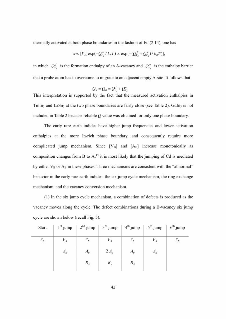
vacancy moves along the cycle. The defect combinations during a B-vacancy six jump

cycle are shown below (recall Fig. 5):

Start 1st jump 2nd jump 3rd jump 4th jump 5th jump 6th jump

BV AV BV AV BV AV BV

BA BA 2 BA BA BA

AB AB AB

43

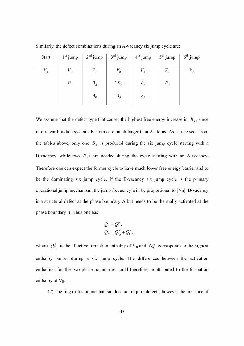
Similarly, the defect combinations during an A-vacancy six jump cycle are:

Start 1st jump 2nd jump 3rd jump 4th jump 5th jump 6th jump

AV BV AV BV AV BV AV

AB AB 2 AB AB AB

BA BA BA

We assume that the defect type that causes the highest free energy increase is AB , since

in rare earth indide systems B-atoms are much larger than A-atoms. As can be seen from

the tables above, only one AB is produced during the six jump cycle starting with a

B-vacancy, while two AB s are needed during the cycle starting with an A-vacancy.

Therefore one can expect the former cycle to have much lower free energy barrier and to

be the dominating six jump cycle. If the B-vacancy six jump cycle is the primary

operational jump mechanism, the jump frequency will be proportional to [VB]. B-vacancy

is a structural defect at the phase boundary A but needs to be thermally activated at the

phase boundary B. Thus one has

6

6

,

,B

mA

f mB V

Q Q

Q Q Q

=

= +

where B

fVQ is the effective formation enthalpy of VB and 6

mQ corresponds to the highest

enthalpy barrier during a six jump cycle. The differences between the activation

enthalpies for the two phase boundaries could therefore be attributed to the formation

enthalpy of VB.

(2) The ring diffusion mechanism does not require defects, however the presence of

44

certain types of defects may facilitate the exchange process. In Zener’s analysis of ring

diffusion in copper13, the energy barrier for the ring exchange mainly arises from the

(non-coulombic) repulsive interaction between positive ions, which could in principle be

reduced by replacing large lattice ions with smaller ones or by taking them away. Since

rare earth atoms are much larger than indium atoms, an antisite defect AB or vacancy VB

could serve to reduce the energy barrier to ring exchange for the twelve A atoms

surrounding it, which may form six 4-ring circles and/or eight 3-ring circles. Moreover,

an AB itself could form twenty-four 3-ring circles with the surrounding A-atoms. If this is

the principal jump mechanism, then Cd jump frequencies should be proportional to [VB]

or [AB]. Like in the six jump cycle mechanism, [VB] and [AB] are abundant as structural

defects at the boundary A but need thermal activation at the boundary B, and one has

,

(or ) ,B B

mA ring

f f mB V A ring

Q Q

Q Q Q Q

=

= +

where mringQ corresponds to the maximal enthalpy increase during a ring rotation. And

the differences between the activation enthalpies for the two phase boundaries could be

attributed to the formation enthalpy of either VB or AB.

(3) The vacancy conversion reaction V + VB A B AA A→ + allows B-vacancies to be

turned into A-vacancies. Even if only a small fraction of B-vacancies are converted, the

so produced A-vacancies may still greatly outnumber thermal A-vacancies at not too high

a temperature at the phase boundary A, where B-vacancies are abundant as structural

defects. One then has

,A

tr mA VQ Q Q= +

45

in which trQ is the transfer enthalpy required for the conversion reaction and A

mVQ is

the migration enthalpy of A-vacancies. At the phase boundary B, A-vacancies still have to

be thermally activated and one has

.A A

f mB V VQ Q Q= +

Therefore for this mechanism the differences between BQ and AQ could be attributed

to A

f trVQ Q− .

All the three mechanisms discussed above would lead to jump frequencies higher

at A boundaries than at B boundaries. However one more condition must be met in order

for these mechanisms to be functioning: that VB or AB must jump at a frequency

comparable to that of Cd. Otherwise part of the Cd probes that are in the vicinity of VB or

AB will jump at a high frequency, while the probes that are away from defects will hardly

jump at all. This would lead to two-signal spectra or significant inhomogeneous

broadening of the spectra, which was not observed in the experiments. The migration of

VB is included in the six jump mechanism. But in the other two mechanisms, the

movement of AB or VB would be difficult as it requires jump distance longer than the

nearest neighbor distance for defects on the A-sites to migrate. Based on this

consideration, the B-vacancy six jump cycle mechanism is most likely to be the

operational mechanism for Cd diffusion in the three early rare earth indides. Calculated

values of QB - QA and interpretations according to the analysis above are given in Table 2.

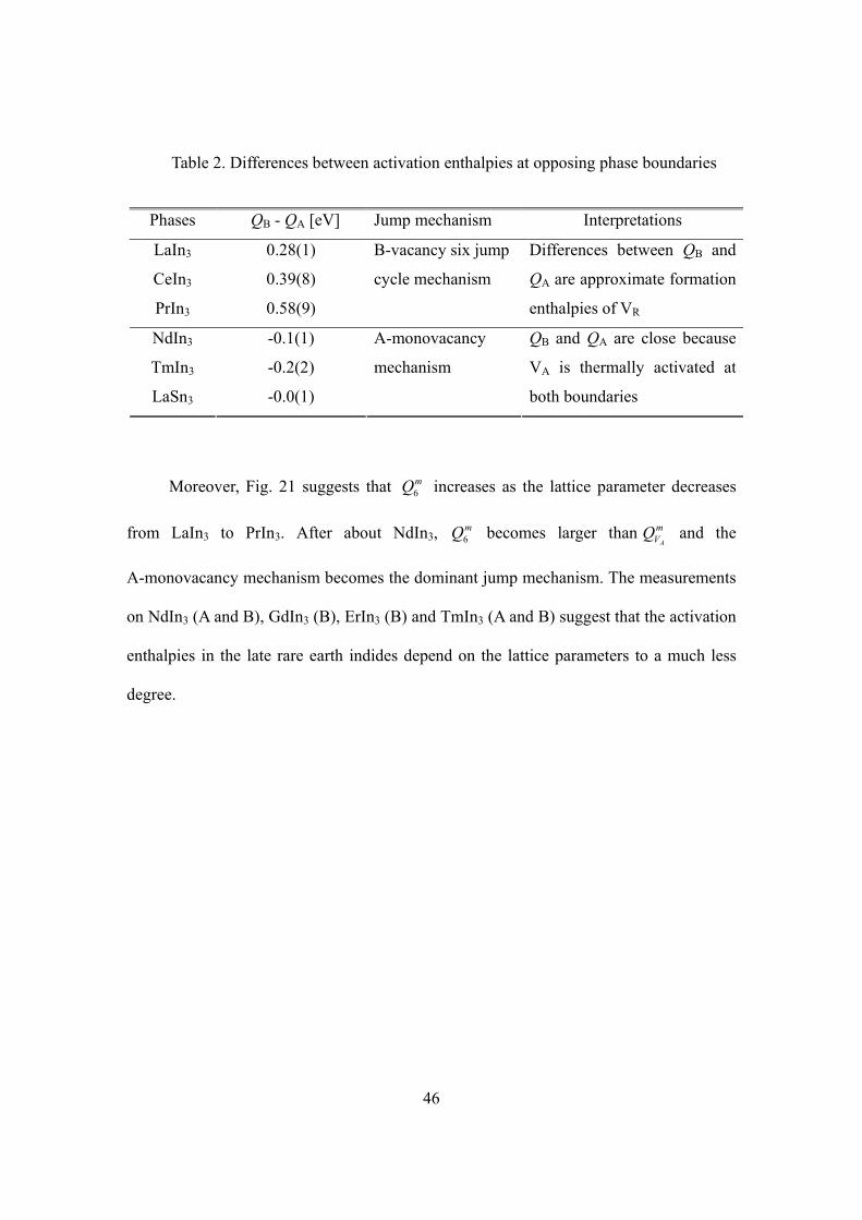
46

Table 2. Differences between activation enthalpies at opposing phase boundaries

Moreover, Fig. 21 suggests that 6mQ increases as the lattice parameter decreases

from LaIn3 to PrIn3. After about NdIn3, 6mQ becomes larger than

A

mVQ and the

A-monovacancy mechanism becomes the dominant jump mechanism. The measurements

on NdIn3 (A and B), GdIn3 (B), ErIn3 (B) and TmIn3 (A and B) suggest that the activation

enthalpies in the late rare earth indides depend on the lattice parameters to a much less

degree.

Phases QB - QA [eV] Jump mechanism Interpretations

LaIn3 0.28(1)

CeIn3 0.39(8)

PrIn3 0.58(9)

B-vacancy six jump

cycle mechanism

Differences between QB and

QA are approximate formation

enthalpies of VR

NdIn3 -0.1(1)

TmIn3 -0.2(2)

LaSn3 -0.0(1)

A-monovacancy

mechanism

QB and QA are close because

VA is thermally activated at

both boundaries

47

6. Summary

Cd jump frequencies were measured in L12 type rare earth indides, gallides and

aluminides, and compared with previous measurements on indides and aluminides. They

were found to span a large range from ~6000 MHz in LaIn3 (A) to less than 1 MHz in

ScAl3 at 1200 K. Activation enthalpies were fitted using the Arrhenius temperature

dependence and were in the range 0.5 – 1.8 MeV, which are low compared with other

metallic systems.

Measurements in rare earth indides were made at the opposing phase boundaries A

and B, which were decided to have compositions that were significantly A-rich or very

close to stoichiometry, respectively, using the free energy curves. A reversal in

composition dependence was seen between the early and late rare earth indides, crossing

over at about NdIn3. GdIn3, TmIn3 and LaSn3 have higher jump frequencies at the less

A-rich boundary, which is in agreement with the widely accepted A-vacancy diffusion

mechanism.

LaIn3, CeIn3 and PrIn3 have lower activation enthalpies at the more A-rich

boundary, which necessitates a more complicated diffusion mechanism. Three

mechanisms were considered to explain the observed behavior, namely the B-vacancy six

jump mechanism, the ring exchange mechanism and the vacancy conversion mechanism.

These mechanisms lead to jump frequencies that are proportional to either [VB] or [AB],

which increase monotonically with In mole fraction. The B-vacancy six jump cycle

mechanism was decided to be the most likely mechanism as a result of the homogeneity

of the spectra. Based on this mechanism, the differences in activation enthalpies at the

48

two phase boundaries, namely 0.28(1) eV for LaIn3, 0.39(8) eV for CeIn3, and 0.58(9) eV

for PrIn3 were attributed to formation enthalpies of rare earth vacancies.

49

References

1 M.O. Zacate, A. Favrot and G.S. Collins, Phys. Rev. Lett. 92 (2004), 225901

2 G.S. Collins, A. Favrot, L. Kang, D. Solodovnikov and M.O. Zacate, Defect and

Diffusion Forum 237-240, 195-200 (2005)

3 H. Mehrer, Mater. Trans. JIM, 37, 1259 (1996)

4 G.S. Collins, A. Favrot, L. Kang, E. Niewenhuis, D. Solodovnikov, J. Wang, and M.O.

Zacate, Hyperfine Interact. 159, 1, (2004)

5 Th. Wichert and E. Recknagel in Microscopic Methods in Metals, U. Gonser (Ed.),

Springer-Verlag Berlin Heidelberg (1986)

6 G. Schatz and A. Weidinger, Nuclear Condensed Matter Physics, J. Gardner (Ed.),

Johns Wiley & Sons (1996)

7 H. Winkler and E. Gerdau, Z. Physik 262, 363 (1973)

8 W. Evenson, J. Gardner, R. Wang, H.-T. Su, and A. McKale, Hyp. Int. 62, 283 (1990)

9 A. Baudry and P. Boyer, Hyp. Int. 35, 803 (1987)

10 H. Mehrer, Diffusion in Solids, Springer-Verlag Berlin Heidelberg (2007)

11 T. Ito, S. Ishioka and M. Koiwa, Philos. Mag. A 62, 499 (1990)

12 M. Koiwa, H. Numakura and S. Ishioka, Defect Diffus. Forum 143-147, 209 (1997)

13 C. Zener, Acta Cryst 3, 346 (1950)

14 G.S. Collins and M.O. Zacate, Hyperfine Interact. 136/137, 641 (2004)

15 E. Nieuwenhuis, Technical report, Lattice locations and diffusion of 111In/Cd atoms in

Ga7Pd3 (2004)

16 S.L.Shropshire, Studies of point defects and defect interactions in metals using

50

perturbed gamma-gamma angular correlations, Ph.D. dissertation, Washington State

University (1991)

17 G.S. Collins, PAC data reduction at WSU, lecture notes (2006)

18 Binary Alloy Phase Diagrams, 2ed edition, T.B. Massalski (Ed.), ASM International

(1990)

19 R. Vianden, Hyp. Int. 15/16, 1080 (1983)

20 G.S. Collins, J. Mater. Sci., 42, 1915 (2007)

21 M. Forker and P. de la Presa, Phys. Rev. B, 76 115111 (2007)

22 J.B. Adams, S.M. Foiles and W.G. Wolfer, J. Mater. Res., 4, 1, 102 (1989)

23 P. Villars and L.D. Calvert, Pearson’s handbook of crystallographic data for

intermetallic phases (1985)