Caching in Ubiquitous Computing Environments: Light and Shadow

5

Caching in Ubiquitous Computing Environments: Light and Shadow

Mianxiong Dong, Long Zheng, Kaoru Ota, Jun Ma, Song Guo, and Minyi Guo

School of Computer Science and Engineering, University of Aizu Japan

1. Introduction

The word ubiquitous [1] means an interface, an environment, and a technology that can

provide all benefits anywhere and anytime without you are aware of what it is, and the

ubiquitous computing is the term which is a concept to let computer exist everywhere in the

real world [2]. In recent years, ubiquitous devices such as RFID, sensors, cameras, T-engine,

and wearable computer have progressed rapidly and have begun to play important roles at

everywhere and at any time in our daily life [3-5]. Although there are potential ubiquitous

applications in nearly every aspect of our world, it is not so easy to build such an

application over infrastructure-less networks.

As our earlier research, we proposed a ubiquitous computing scenario which consists of

many heterogeneous processing nodes, named Ubiquitous Multi-Processor (UMP).We

introduced a basic framework of multiprocessor simulator system based on a multi-way

cluster for the research of heterogeneous multiprocessor system with both high scalability

and high performance [6]. The objective of [6] is to organize a basic simulator system

framework. Furthermore, as the next step, we proposed and implemented a double-buffered

communication model to improve communication speed keeping independence from each

processor model on the system. The proposed model showed over 50% system performance

improvement rate compared with the basic framework integrated with the single-buffered

model [7]. As the further stage of the hardware simulation, we implemented a ubiquitous

multi-processor network based pipeline processing framework to support the development

of high performance pervasive application [8]. In [8], we also developed a distributed JPEG

encoding application successfully based on the proposed framework. Based on these

previous researches, the next work would be improving the performance of the UMP

system. In the research of the evaluation of the network transmission speed [13-14], we

focused on the performance of the network communication part of the UMP system.

Through our experiment, we have found the best way to decide the packet size of the UMP

network.

Continuously to [13-15] in this article we evaluated four algorithms of the UMP system

which the purpose is to find an optimal solution considering the loading balance of the

Resource Router, total execution time, execution efficiency and task waiting time (delay).

www.intechopen.com

Ubiquitous Computing

96

2. An overview of the ubiquitous multi-processor system

The final goal of the UMP project is to provide a network framework for the coming ubiquitous society. In the ubiquitous society, services could be likened the air, i.e., they will exist everywhere and anytime to meet each user's request. In order to fill such requests, computing resources are necessarily provided under two conflicting conditions: higher performance and lower power consumption. To this end, we have proposed the UMP system which is introduced in detail in this section.

2.1 Software architecture of UMP system

Fig. 1. UMP system overview

Fig. 1 is an overview of the UMP system. In our system, there are three kinds of nodes. One is the Client Node which works instead of the mobile users. This node requests tasks through mobile terminals on a wireless network. The other is the Resource Router (RR) which is a gateway of the system. There exists only one node of RR in one subnet. This node received task requests from the Client Nodes. Then, the node manages a list of tasks and determines which tasks should be executed currently on the subnet. The last one is the Calculation Node which actually executes tasks requested from the Client Nodes. Every task is allocated by the RR on the subnet. When a task is executed, several Calculation Nodes are connected to each other like a chain. For example, to encode a bitmap file into JPEG file, the whole steps are six. So it means the chain has six Calculation Nodes. Combination of the Calculation Nodes is always unique so that actions of tasks can be changed flexibly by the demands of the Client Nodes. We call the Calculation Nodes as Processing Elements (PEs) afterwards.

www.intechopen.com


97

2.2 Motivation of our work

As a case study of the UMP system, we implemented a prototype application of the JPEG

encoding [8]. The application is developed to convert bitmap format image to JPEG format

image. At that stage, the implementation was simple and the algorithm of the processing

schedule was not considered enough. The scale of the prototype system was small; it

couldn’t server a large request of tasks. In the real world, many users will request the

service/task at simultaneously to the UMP system. So, it is obviously optimizing the time

efficiency, loading balance of the RR, reducing the delay of task execution, total execution

time of the whole task are pressing needs. Of course, there is a trade off between these

factors. How to design the UMP system to meet the providing of the real service is a

challenge thing. Generally speaking, processing speed would be quite faster than network

speed in usual. One of benchmarks of network performance is the network overhead [9]. In

[13-14], we compared processing time of using stand-alone application to processing time of

using UMP system. The result shows the difference between processing time of the former

and later is network overhead time. So, increasing the usage of each PE is one way to

generate the good performance. In other words, assign tasks as much as possible under the

limitation of the processing ability and reducing the communication cost.

3. Resource allocation algorithms for the resource router

In this section, we introduce two resource allocation algorithms for the RR to find single PE whose state is idle. Resource allocating should be optimized since time consumption for that is not trivial over total execution time. We propose an optimized algorithm and evaluate it by probability analysis. Resource allocation algorithms with multi PEs are also introduced in the following section 4.

3.1 Basic algorithm for the RR to search idle PEs

The RR has a role to look for a PE necessary to execute a task as the following steps.

1. The RR searches an idle PE randomly and sends a PE a message to check its state. 2. The PE sends the RR an answer of idle/busy. 3. After the RR gets the answer of idle, it finishes the search. If the answer is busy, back to

(1) and continue.

Firstly, the RR randomly searches a PE in a state of the idle by sending a message to ask a PE whether the PE is in an idle state or a busy state. The PE replies to the RR with its current state when it receives the message. When a response from PE is an idle state, the RR sends the PE a message to request execution of the task. Otherwise, the RR looks for other available PE. It keeps retrieving idle PEs until the execution of all tasks ends. We can consider two possible scenarios for the RR to search an idle PE: the best case and the

worst case. The best case means the RR successfully finds an idle PE at the first search, i.e.,

the first retrieved PE is in the idle state so that the RR no longer looks for other PE. In

contrast, the worst case means the RR finds an idle PE after searching every PE on the

subnet, i.e., it retrieves the idle PE at last although the all other PEs are busy.

In the basic algorithm, the RR looks for an available PE at random. Therefore, the best case can be not always expected and the worst case cannot be avoided. One reason for the worst

www.intechopen.com


98

case is there exist PEs being often in the busy state. A long delay can be generated if the RR keeps retrieving such a busy PE instead of other idle ones. We consider that if the RR omits such PEs to retrieve, it can find an idle PE quickly and efficiently. The basic idea can be described as follows: 1) firstly making a group of PEs being often in a busy state, and 2) the RR does not retrieve any PE from the group. A concrete method is needed for finding such busy PEs and presented in the following subsection.

3.2 Optimized algorithm

In the optimized algorithm, firstly the RR searches an idle PE randomly and checks each PE's state. After the RR repeats this procedure many times, it makes a group of busy PEs based on a history of each PE's state the RR checked. In the next search, the RR tries to find an idle PE excluding from the group. If the RR cannot find any idle PE, it searches an idle PE from inside and outside of the group. This algorithm is based on an assumption that there exists at least one idle PE of all. Details of the algorithm are described as the following steps.

1. The RR secures a storage region of each PE to save its degree of idle state, which starts from 0. 2. The RR searches an idle PE randomly and sends a PE a message to check its state. 3. The PE sends the RR an answer of idle/busy. 4. If the RR gets the answer of idle from the PE, it finishes the search and the PE's degree

of busy state is decremented by 1. If the answer is busy, the PE's degree is incremented by 1 and the RR searches the next PE.

5. If repeating from Step 2 to Step4 $s$ times, the RR looks into each PE's storage. If a PE's degree of busy state is more than a threshold, the PE is regarded as ``PE with high probability of busy''

6. After the end of looking into storages, the RR makes a group of PEs with high probability of busy.

7. The RR searches an idle PE again expect for PEs belonging to the group $t$ times. If the RR cannot find any idle PE, it begins to search for an idle PE including inside of the group.

8. Step5-7 are repeated until the entire search ends.

In the optimized algorithm, we can also consider the best case and the worst case for the RR to spend time for searching an idle PE. The best case can occur when the RR finds an idle PE at the first search like the best case of the basic algorithm. On the other hand, the worst case is the RR firstly searches an idle PE from outside of the group but all PEs are in the busy state. Hence, the RR starts to look for an idle PE from the group and then it finally finds an idle PE after the all other PEs in the group are queried by the RR.

3.2 Probability analyses and discussion

As the first stage, we evaluate the optimized algorithm with probability analyses using

probabilities of finding an idle PE in the best case and the worst case with the basic

algorithm and the optimized algorithm respectively. Both probabilities depend on

probabilities of a PE in an idle state and a busy state respectively.

We use the queuing theory \cite{11} to obtain the probabilities of a PE in an idle state and a

busy state. The queuing theory is used to stochastically analyze congestion phenomena of

queues and allows us to measure several performances such as the probability of

www.intechopen.com


99

encountering the system in certain states like idle and busy. Here, we consider one PE as on

one system and then its queuing model can be described as M/M/1(1) by Kendall's

notation. That means each PE receives a message from the RR randomly and deals with only

one task at once. Hence, when a PE processes a task and at same time a message comes from

the RR, the message is not accepted by the PE because of the busy state.

P0 Probability that a PE is in an idle state where $0 \leq P_0 \leq 1$.

P1 Probability that a PE is in a busy state where $P_1=1-P_0$.

n The total number of PEs in a subset.

m Number of PEs in the group (regarded as a PE with high

probability of busy).

P’1 Probability that a PE in the group is busy.

λ Average arrival rate of a message from the RR to a PE.

μ Average task execution rate of a PE.

ρ Congestion condition.

'ρ Congestion condition of the group

Table 1. The notations used in equations

Before the analysis, some notations are defined in Table 1. Equation (1) and (2) show the

probabilities of finding an idle PE from one subnet in the best case and the worst case

respectively when the basic algorithm is used.

In the best case of the probability of finding an idle PE:

P = P0 (1)

In the worst case of the probability of finding an idle PE:

( 1)1

nP P −= (2)

On the other hand, Equation (3) and (4) show the probabilities of the best case and the worst

case respectively when the optimized algorithm is used. Here, we have new notations as

follows.

In the best case of the probability of finding an idle PE:

P = P0 (3)

In the worst case of the probability of finding an idle PE:

( ) ( 1)1 1*n m mP P P− −= (4)

The best case is just the same as the one using the basic algorithm since the RR finds an idle

PE at the first search in the both algorithms. Therefore, we consider only the worst cases to

comparing the optimized algorithm with the basic algorithm.

The range of m in the worst case, since PEs in the group is a part of all PEs in the subnet, can

be 0 m n≤ ≤ . In the case of m=0 or m=n, it is just the same as the worst case using the basic

www.intechopen.com


100

algorithm. Moreover, we assume 1 1'P P< since PEs in the group are regarded as PEs with

high probability of busy and should encounter a busy state more than else PEs in the subnet. From the queuing theory,

1 (1 )P ρ ρ= − (5)

'1 '(1 ')P ρ ρ= − (6)

A notation ρ can be calculated as

/ρ λ μ= (7)

And 'ρ in Equation (6) shows the congestion condition of a PE in the group. We also

assume 'ρ ρ< from the condition 1 1'P P< as mentioned before.

Here we can consider ρ as each PE's degree of busy state, since the RR classifies PEs based

on the degree by comparing with a threshold decided beforehand. Therefore, 'ρ of all PEs

in the group should be more than or equal to the threshold, so that thresholdρ < for other

PEs. To always keep these conditions, we assume ' thresholdρ = and simply fixed the

relation between 'ρ and ρ as follows.

' 0.1ρ ρ= + (8)

where 0.1 0.9ρ< < and 0.2 ' 1.0ρ< < with considering possible values of threshold in a

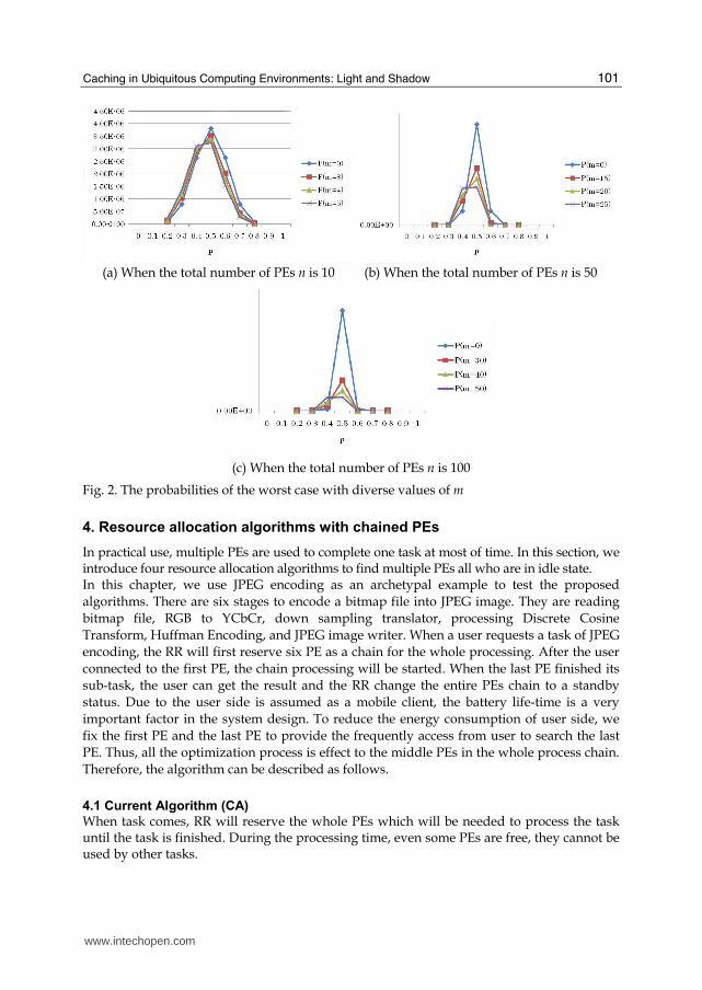
practical use. Based on the assumption, we obtain the probabilities of the worst case in the basic algorithm and the optimized algorithm using the Equation (2) and the Equation (4) respectively. Fig. 2 shows the probabilities with changing n, the total number of PEs in a subnet, from 10 to 100. In each case of n, we also change m, the number of PEs in the group, from 0% to 50% of n. When m is 0% of n, i.e., m=0 in Fig. 2, that means the basic algorithm is applied since there is no PE in the group. For example, Fig. 2(a) shows the probabilities of the worst case for each m from 0 to 5 with n=10.

In Fig. 2, we focus on the three parameters which are ρ , n, and m for discussion of the

results. Firstly, when 0.4 0.8ρ< < , the probabilities where m>0 become lower than one

where m=0 in most cases, so that the threshold of ρ should be set to more than 0.5 and less

than 0.9 to avoid the worst case using the optimized algorithm. Secondly, the more the total number of PEs n, the bigger difference of the probabilities between the basic algorithm (m=0) and the optimized algorithm (m>0) as shown in Fig. 2. Therefore, we can conclude the optimized algorithm has less risk of the worst case than the basic algorithm as the total number of PEs is larger. Finally, the number of PEs in the group m gives less impact on results comparing to other two parameters. However, in Fig. 2, we can see slightly less probabilities of the worst case as m is larger. As a result, using the optimized algorithm encounters the worst case less than using the basic algorithm if the following conditions are met; (1) the threshold to make a busy group by checking of each PE ranges from 0.6 to 0.8, and (2) the total number of PEs in a subnet is relatively large. Considering these two conditions in implementation, effective performance using the optimized algorithm can be expected.

www.intechopen.com


101

(a) When the total number of PEs n is 10 (b) When the total number of PEs n is 50

(c) When the total number of PEs n is 100

Fig. 2. The probabilities of the worst case with diverse values of m

4. Resource allocation algorithms with chained PEs

In practical use, multiple PEs are used to complete one task at most of time. In this section, we introduce four resource allocation algorithms to find multiple PEs all who are in idle state. In this chapter, we use JPEG encoding as an archetypal example to test the proposed algorithms. There are six stages to encode a bitmap file into JPEG image. They are reading bitmap file, RGB to YCbCr, down sampling translator, processing Discrete Cosine Transform, Huffman Encoding, and JPEG image writer. When a user requests a task of JPEG encoding, the RR will first reserve six PE as a chain for the whole processing. After the user connected to the first PE, the chain processing will be started. When the last PE finished its sub-task, the user can get the result and the RR change the entire PEs chain to a standby status. Due to the user side is assumed as a mobile client, the battery life-time is a very important factor in the system design. To reduce the energy consumption of user side, we fix the first PE and the last PE to provide the frequently access from user to search the last PE. Thus, all the optimization process is effect to the middle PEs in the whole process chain. Therefore, the algorithm can be described as follows.

4.1 Current Algorithm (CA)

When task comes, RR will reserve the whole PEs which will be needed to process the task until the task is finished. During the processing time, even some PEs are free, they cannot be used by other tasks.

www.intechopen.com


102

The characteristic of the current resource allocation algorithm can be analyzed into two parts: i. Mean delay:

/

1

1( 1) ( / ) /

n m

i

d m i t n n m m n m tn

⎢ ⎥⎣ ⎦=

⎛ ⎞⎜ ⎟= ⋅ − + − ⋅⎢ ⎥ ⎢ ⎥⎣ ⎦ ⎣ ⎦⎜ ⎟⎝ ⎠∑ (9)

where m is the number of tasks RR can handle at one time, t is the time to handle m tasks. So the first m tasks wait 0 time, the second m tasks wait t time, the i-th m tasks should wait (i-1)t time. We can also get task execution efficiency as follows:

ii. Task Execution Efficiency:

1

, 11 1 1

n n n

i i i ii i i

f e e c−

+= = =⎛ ⎞= +⎜ ⎟⎜ ⎟⎝ ⎠∑ ∑ ∑ (10)

Where ei (1 ≤ i ≤ n) is the execution time in i-th PE, , 1j jc + is the communication time

between j-th PE and (j+1)-th (1 ≤ j ≤ n) PE. In our simulation, we assume the communication time between any two PEs is the same, i.e.

, 1 , , , ,j j m nc c c i j m n N+ = = ∀ ∈ , N is the natural number set. Hence,

1 1

( 1)n n

i ii i

f e e n c= =

⎛ ⎞= + − ⋅⎜ ⎟⎜ ⎟⎝ ⎠∑ ∑ (11)

Abstract of the CA is described as follows.

1. Router retrieves a new task from the task queue. If there is no task in the task queue, then ends.

2. Router generates a PE chain which is used to process a task. Set the PEs in the PE chain as busy, which means these PE can not do any other task until they are released.

3. Router sends the PE chain information and task to PE1. 4. PE1 finishes its work and follows the PE chain information to transfer the task to PE2. 5. PE2 finishes its work and follows the PE chain information to transfer the task to PE3. 6. PE4 finishes its work and follows the PE chain information to transfer the task to PE5. 7. PE5 finishes its work and follows the PE chain information to transfer the task to PE6. 8. PE6 finishes its work and sends the processed task back to router. 9. Router sets all PEs in the PE chain as idle. 10. Remove the task from the task queue. If there is no task left in the task queue, then

terminates. Otherwise go to Step (1).

4.2 Randomly Allocating Algorithm (RAA)

The biggest limitation of the current policy is that if the RR allocates the PEs to the users once, the all PEs are reserved until the whole task will be finished. This is obviously a big useless of the computational resource. To regard as this point, we apply a randomly distribute algorithm to the UMP system. The concept of RAA is after the PE finished the

www.intechopen.com


103

execution of the process, the PE will ask the RR for the next phase of PE. The usage rate of PE is quite high, but the load balance is heavy for the RR. We can get task execution efficiency as follows: i. Task execution efficiency:

1

1,1 1 1 2

n n n n

i i i i ii i i i

f e e cr c−

−= = = =⎛ ⎞= + +⎜ ⎟⎜ ⎟⎝ ⎠∑ ∑ ∑ ∑ (12)

where niei

≤≤1 , is the execution time, nicii

≤≤− 2,1 is the communication time between i-th

PE and RR, nicri

≤≤1 is the communication time between (i-1)-th PE and i-th PE. Abstract of the RAA is described as follows.


2. Router finds an idle PE1 and any PE6 and then transfers the task to this PE1. 3. After getting the task from router, this PE1 sends a busy status message to router. 4. After processing the task, this PE1 send an idle status message to router and meantime

ask the router for the next PE. 5. Router finds an idle PE2, and then tells the PE1. 6. PE2 sends the status busy to router; PE1 transfers the task to PE2, and sends idle status

message to router. 7. PE2, PE3, PE4 act the same. 8. After PE5’s processing the task, PE5 transfers the task the PE6 which is decided by

router at Step 2. 9. After PE6’s processing the task, transfer the processed task back to router. 10. Remove the task from the task queue. If there is no task left in the task queue, then


4.3 Randomly Allocating Algorithm with Cache technology (RAA-C).

To improve the RAA, we introduce a cache concept of the resource allocating algorithm. For every PE, we assign a cache for them to memorize the next stage’s PE. When they finished their sub-task, they will search the next phase of PE in their cache. If the all PEs in the cache are at the busy status, it will ask RR to assign one free PE as the next phase PE. We can get task execution efficiency as follows: i. The best case of task execution efficiency:

1,1 1 2

(3 )n n n

i i i ii i i

f e e c −= = =⎛ ⎞= +⎜ ⎟⎜ ⎟⎝ ⎠∑ ∑ ∑ (13)

where niei

≤≤1 is the execution time, nicii

≤≤− 2,1 is the communication time between (i-1)-th

PE and i-th PE. The best case means each (i-1)-th PE can access each i-th PE memorized in their cache because i-th PE is not busy. (i-1)-th PE is supposed to have communication with i-th PE three times in total. As the first communication, (i-1)-th PE asks i-th PE whether or not it is busy currently. Then, i-th PE replays to (i-1)-th PE in the second communication. Since this is the best case so that i-th PE’s answer must be “available”, (i-1)-th PE starts to send data to i-th PE in the third communication.

www.intechopen.com


104

ii. The worst case of task execution efficiency:

1

1,1 1 2 1

(3 )n n n n

i i i i ii i i i

f e e c cr−

−= = = =⎛ ⎞= + +⎜ ⎟⎜ ⎟⎝ ⎠∑ ∑ ∑ ∑ (14)

where niei

≤≤1 is the execution time, 11 −≤≤ nicri is the communication time between i-th

PE and RR, nicii

≤≤− 2,1 is the communication time between (i-1)-th PE and i-th PE. The worst

case means each (i-1)-th PE cannot access each i-th PE memorized in their cache because i-th

PE is busy. Therefore, each (i-1)-th PE has to ask RR for a free PE. Abstract of the RAA-C is described as follows.

1. Router retrieves a new task from the task queue. If there is no task in the task queue,

then ends.

2. Router finds an idle PE1 and any PE6 and then transfers the task to this PE1.

3. After getting the task from router, this PE1 sends a busy status message to router.

4. After processing the task, this PE1 sends an idle status message to router.

5. Find the idle PE from its cache.

6. If the PE1 finds an idle PE2, then send a request message to verify whether the PE2 is

truly idle or not.

7. If the response from PE2 is yes, then go to step 10; or send a request message to router,

by which router will look for an idle PE2 without restriction of PE1’s cache.

8. If router finds one, then tell PE1, otherwise, repeat steps from Step (5).

9. Router finds an idle PE2, and then tells the PE1.

10. PE2 send the busy status message to router; PE1 transfers the task to PE2, and then

sends the idle status message to router.

11. PE2, PE3, PE4 act the same, besides updates the information of cache of PE1, PE2, PE3,

respectively.

12. After PE5’s processing the task, PE5 updates the information of cache of PE4; and then

transfers the task the PE6 which is decided by router at Step 2.

13. After PE6’s processing the task, transfer the processed task back to router.

14. Remove the task from the task queue. If there is no task left in the task queue, then


4.4 Randomly Allocating Algorithm with Grouping method (RAA-G).

The RAA-G is slightly different from RAA-C. We use a grouping method to group the PEs.

The difference between the RAA-G and RAA-C is the restriction of jumping to the PEs

which is out of the cache that current PE has. That means when a certain PE finished its sub-

task and the whole PEs in the cache (group) are busy, the PE will not ask RR to assign a free

PE out of the cache. For example, assume every cache at each phase has four PEs. When a

certain PE at one stage finished the sub-task, it can search the next phase PE in the same

cache. If the next phase PE is all busy status, it has to wait. This is the biggest difference

between RAA-C and RAA-G. And the Efficiency of RAA-G in the best case is the same to

RAA-C. Here, the best case means each (i-1)-th PE succeeds to find the next phase PE in only

one access without asking all PE members in the cache.

www.intechopen.com


105

i. The worst case of task execution efficiency:

1, 1,1 1 2 1

2n n n l

i i i j i ii i i j

f e e c c− −= = = =⎛ ⎞⎛ ⎞⎜ ⎟⎜ ⎟= + +⎜ ⎟⎜ ⎟⎝ ⎠⎝ ⎠∑ ∑ ∑ ∑ (15)

where 1ie i n≤ ≤ is the execution time, 1, 2i ic i n− ≤ ≤ is the communication time between (i-1)-

th PE and i-th PE, 1, 2 ,1i ijc i n j l− ≤ ≤ ≤ ≤ where l is the number of PEs in one group, is also the

communication time between (i-1)-th PE and i-th PEs in the group. The worst case means each

(i-1)-th PE asks all next phase PEs in a group at every stage. It is because (i-1)-th PE checks

whether or not PE in the group is busy one by one in order to seek one available PE. Abstract of the RAA-G is described as follows.


2. Router finds an idle PE1 and any PE6 and then transfers the task to this PE1. 3. After getting the task from router, this PE1 sends a busy status message to router. 4. After processing the task, this PE1 sends an idle status message to router. 5. Find the idle PE from its cache. 6. If the PE1 finds an idle PE2, then send a request message to verify whether the PE2 is

truly idle or not. 7. If the response from PE2 is yes, then go to step 10; or waits a particular time, then go to

step 5. 8. PE1 transfers the task to PE2. 9. PE2, PE3, PE4 act the same, besides updates the information of cache of PE1, PE2, PE3,

respectively. 10. After PE5’s processing the task, PE5 updates the information of cache of PE4; and then

transfers the task the PE6 which is decided by router at Step (2). 11. After PE6’s processing the task, transfer the processed task back to router. 12. Remove the task from the task queue. If there is no task left in the task queue, then


4.5 Performance evaluation and discussion

We built a simulation system to evaluate the 4 algorithms. We used the Poisson Distribution to generate the tasks because the Poisson Distribution arises in connection with Poisson processes. It applies to various phenomena of discrete nature (that is, those that may happen 0, 1, 2, 3, ... times during a given period of time or in a given area) whenever the probability of the phenomenon happening is constant in time or space. After run the generator, we got 291 tasks for the evaluation. And we set 240 PEs. Each processing needs 6 PEs, therefore the total chains of PEs are 40. We also set the network delay as 100. Table 2 shows the environment of the simulation. Fig. 3 shows the loading balance of RR from the simulation result. We can see the sum loading balance of CA and RAA-G perform a good result because the algorithms their self restrict the communication with RR. And it is naturally the RAA had worst result, because almost every time the PE should ask RR to know the next phase PE which should be connected to.

www.intechopen.com


106

OS Windows Vista Business (32-bit)

CPU AMD Athlon64 3200+

Memory DDR SDRAM 2GB

Language JAVA 1.5

Network Localhost

Table 2. The experiment environment

Fig. 3. The loading balance of RR of four algorithms

www.intechopen.com


107

Fig. 4. The efficiency of tasks

Fig. 4 is a distribution view of efficiency of tasks. Because the efficiency is highly related

with the communication cost, CA shows a best result as well as it doesn’t have much

communication with RR and the other PEs. The average efficiency of RAA-C and RAA-G

are almost the same, it is perfect matching the mathematic model we have described above.

RAA also has a better result than RAA-C and RAA-G. But consider the loading balance of

RR it is still not acceptable.

www.intechopen.com


108

From the left part of Fig. 5, we can see the proposed algorithms have a significant

improvement compared with the current implementation. Also, from the right part of Fig. 5,

we can see the RAA-G and RAA-C are slightly performing a good result than RAA.

Fig. 5. The total processing time of the tasks

5. Conclusion

In this chapter, we propose an optimized algorithm for resource allocation to a processing

node, which can improve the overall performance of the UMP system. Using the optimized

algorithm, the RR can effectively find a single PE in an idle state, which actually can process

an assigned task. As a result, the RR saves the time to search for an idle node so that total

performance of resource allocation can be improved. Finally, we evaluated the optimized

algorithm with probability analyses and figured out conditions for the optimized algorithm

to be better than the basic algorithm.

Also, as the further step our previous works, we evaluated the performance with four

different resource (PE) allocating algorithm for multiple PEs and analyzed these algorithms

from three points of view. Though these huge experiments, we have successfully proofed

our proposed algorithms are meaning while. Considering those three key factors (the time

efficiency, loading balance of the RR, and total processing time of the whole task), each

algorithm has its merit and demerit. There is always a trade off between these factors.

Taking into account the balanced point of all factors, we found the RAA-G is the best

algorithm to allocating resources (PEs) when the condition is the system has many users and

many task to process. The next better algorithm is RAA-C, following by RAA. For other

cases, it is difficult to say which algorithm is the best, because it is truly case by case. One

more things we have realized through the experiments are we can set the allocating policy

flexibly answering to the user’s request. Maybe that is the best solution to design the UMP

system. In the future, we will focus on the above layer of the UMP system - the service layer,

to deal with the context information from users, resources and environments.

www.intechopen.com


109

4. Acknowledgment

This work is supported in part by Japan Society for the Promotion of Science (JSPS) Research Fellowships for Young Scientists Program, JSPS Excellent Young Researcher Overseas Visit Program, National Natural Science Foundation of China (NSFC) Distinguished Young Scholars Program (No. 60725208) and NSCF Grant No. 60811130528.

5. References

[1] M. Weiser, “The Computer for the 21st Century,” Scientific Am., pp. 94-104, September,

1991.; reprinted in IEEE Pervasive Computing, pp. 19-25, January-March 2002.

[2] Wikipedia, the free encyclopedia, http://ja.wikipedia.org/wiki/

[3] M. Satyanarayanan, “Pervasive Computing: Vision and Challenges”, IEEE Personal

Communication, pp. 10-17, August 2001.

[4] S. R. Ponnekanti, et.al, "Icrafter: A service framework for ubiquitous computing

environments", In Proc. of Ubicomp 2001, pp. 56–75, Atlanta, Georgia, October

2001.

[5] V. Stanford, “Using Pervasive Computing to Deliver Elder Care”, IEEE Pervasive

Computing, pp. 10-13, January-March, 2002.

[6] A. Shinozaki, M. Shima, M. Guo, and M. Kubo, "A High Performance Simulator System

for a Multiprocessor System Based on a Multi-way Cluster", Advances in Computer

Systems Architecture, Lecture Notes in Computer Science vol. 4186, pages 231-243,

Springer Berlin/Heidelberg, September, 2006.

[7] A. Shinozaki, M. Shima, M. Guo, and M. Kubo, “Multiprocessor Simulator System Based

on Multi-way Cluster Using Double-buffered Model”, Proceeding of AINA 2007,

Niagara Falls, Canada, May 2007, pp. 893-900.

[8] M. Kubo, B. Ye, A. Shinozaki, T. Nakatomi and M. Guo, “UMP-PerComp: A Ubiquitous

Multiprocessor Network-Based Pipeline Processing Framework for Pervasive

Computing Environments”, Proceeding of AINA 2007, Niagara Falls, Canada, May

2007, pp. 611-618.

[9] Wikipedia, the free encyclopedia, ”Computational overhead”, Available:

http://en.wikipedia.org/wiki/Computational overhead.

[10] Wikipedia, the free encyclopedia, ”Maximum transmission unit”,

http://en.wikipedia.org/wiki/Maximumtransmissionunit.

[11] Microsoft, ”Default MTU Size for Dierent Network Topology”, Knowledge Base Article,

ID.140375.

[12] Lawrence S. Husch and University of Tennessee, Knoxville, Mathematics Department,

”Horizontal Asymptotes”,

http://archives.math.utk.edu/visual.calculus/1/horizontal.5/.

[13] M. Dong, S. Guo, M. Guo and S. Watanabe, “Design of the Ubiquitous Multi-Processor

System Focusing on Transmission Data Size”, In Proc. of HPSRN, pp. 158-166,

Sendai, Japan, March 2008

[14] M. Dong, S. Watanabe, and M. Guo, “Performance Evaluation to Optimize the UMP

System Focusing on Network Transmission Speed”, In Proc. of FCST, pp. 7-12,

Wuhan, China, November 2007

www.intechopen.com


110

[15] M. Dong, M. Guo, L. Zheng, S. Guo, “Performance Analysis of Resource Allocation

Algorithms Using Cache Technology for Pervasive Computing System”, in

Proceedings of ICYCS 2008, pp. 671-676, November 2008

www.intechopen.com

Ubiquitous ComputingEdited by Prof. Eduard Babkin

ISBN 978-953-307-409-2Hard cover, 248 pagesPublisher InTechPublished online 10, February, 2011Published in print edition February, 2011

InTech EuropeUniversity Campus STeP Ri Slavka Krautzeka 83/A 51000 Rijeka, Croatia Phone: +385 (51) 770 447 Fax: +385 (51) 686 166www.intechopen.com

InTech ChinaUnit 405, Office Block, Hotel Equatorial Shanghai No.65, Yan An Road (West), Shanghai, 200040, China

Phone: +86-21-62489820 Fax: +86-21-62489821

The aim of this book is to give a treatment of the actively developed domain of Ubiquitous computing.Originally proposed by Mark D. Weiser, the concept of Ubiquitous computing enables a real-time globalsensing, context-aware informational retrieval, multi-modal interaction with the user and enhancedvisualization capabilities. In effect, Ubiquitous computing environments give extremely new and futuristicabilities to look at and interact with our habitat at any time and from anywhere. In that domain, researchers areconfronted with many foundational, technological and engineering issues which were not known before.Detailed cross-disciplinary coverage of these issues is really needed today for further progress and wideningof application range. This book collects twelve original works of researchers from eleven countries, which areclustered into four sections: Foundations, Security and Privacy, Integration and Middleware, PracticalApplications.

How to referenceIn order to correctly reference this scholarly work, feel free to copy and paste the following:

Mianxiong Dong, Long Zheng, Kaoru Ota, Jun Ma, Song Guo and Minyi Guo (2011). Caching in UbiquitousComputing Environments: Light and Shadow, Ubiquitous Computing, Prof. Eduard Babkin (Ed.), ISBN: 978-953-307-409-2, InTech, Available from: http://www.intechopen.com/books/ubiquitous-computing/caching-in-ubiquitous-computing-environments-light-and-shadow

© 2011 The Author(s). Licensee IntechOpen. This chapter is distributedunder the terms of the Creative Commons Attribution-NonCommercial-ShareAlike-3.0 License, which permits use, distribution and reproduction fornon-commercial purposes, provided the original is properly cited andderivative works building on this content are distributed under the samelicense.

https://creativecommons.org/licenses/by-nc-sa/3.0/

Documents

Caching in Ubiquitous Computing Environments: Light and Shadow