Embed Size (px)
Citation preview

Cable Stay Fatigue Analysis for the
Fred Hartman Bridge
by
John C. Eggers, B.S.C.E.
Thesis
Presented to the Faculty of the Graduate School of
The University of Texas at Austin
in Partial Fulfillment
of the Requirements
for the Degree of
Master of Science in Engineering
The University of Texas at Austin
August 2003

Cable Stay Fatigue Analysis for the
Fred Hartman Bridge
Approved by Supervising Committee:
Dr. Sharon Wood, Supervisor
Dr. Karl Frank, Supervisor

Dedication
I would like to dedicate this thesis to my parents, my father and mother in-
law, and my beautiful, patient, and loving wife, Jennifer.

iv
Acknowledgements
I would like to thank the Texas Department of Transportation for
sponsoring this project at the Ferguson Structural Engineering Laboratory (FSEL)
at The University of Texas at Austin.
I would like to also give my appreciation to the many professors that
assisted in my research. Specifically I would like to thank Dr. Sharon Wood and
Dr. Karl Frank for their advice and dedication to this project.
A large amount of manual labor was required for this project. I would like
to thank Tammer Botros and Meg Warpinski for their companionship, labor, and
ideas throughout the project. The lab technicians who include Blake Stassney,
Mike Bell, and Dennis Fillip provided invaluable assistance throughout the
project. Their experience and knowledge of the laboratory environment provide
an enormous amount of assistance to every research project at FSEL.
I would also like to thank my fellow graduate students for making life at
FSEL and The University of Texas enjoyable.
May 2003
v
Abstract
Cable Stay Fatigue Analysis for the
Fred Hartman Bridge
John C. Eggers, M.S.E.
The University of Texas at Austin, 2003
Supervisors: Sharon Wood, Karl Frank
Topics covered in this thesis include analysis and testing of single-strand specimens under tension and static bending loads, including the development of closed-form solutions to estimate the bending moment in a single strand under tension and bending. It also includes tensile fatigue characterization of strand. In addition, there is the characterization and analysis of vibration data from the Fred Hartman Bridge, including integration of acceleration data to attain displacement records and rainflow cycle counting analyses.

vi
Table of Contents
CHAPTER 1 INTRODUCTION ...............................................................................1
1.1 Fred Hartman Bridge ......................................................................................1
1.2 Cable Vibration Problems ..............................................................................3
1.3 Research Conducted at The University of Texas ...........................................5
1.3.1 Field Measurments ................................................................................5
1.3.2 Full-Scale Bending Fatigue Testing ......................................................6
1.3.3 Computational Models ..........................................................................7
1.4 Topics Covered in this Thesis ........................................................................7
1.4.1 Single Strand Bending Tests .................................................................7
1.4.2 Fatigue Tests of Strand in Tension........................................................8
1.4.3 Characterization of Cable Vibration Data from the Fred Hartman Bridge 8
CHAPTER 2 SINGLE-STRAND BENDING TESTS ...............................................10
2.1 Introduction ..................................................................................................10
2.2 Closed-form Solutions ..................................................................................11
2.2.1 Fixed End Beam Subjected to Axial Tension and Bending ................14
2.2.2 Simply-Supported Beam Subjected to Axial Tension and Bending ...16
2.3 Single-strand Tests .......................................................................................17
2.3.1 Test Apparatus .....................................................................................18
2.3.2 Measured Response .............................................................................20

vii
2.4 Comparison of Measured and Calculated Response ....................................28
2.4.1 Stiffness Comparison...........................................................................28
2.4.2 Moment Comparison...........................................................................31
2.5 Summary 33
CHAPTER 3 STRAND TENSION FATIGUE TEST ...............................................35
3.1 Introduction ..................................................................................................35
3.2 Test Program ................................................................................................35
3.2.1 Test Set-up ...........................................................................................36
3.2.2 Aluminum Clamps...............................................................................37
3.3 Results 41
CHAPTER 4 CHARACTERIZATION OF CABLE VIBRATION DATA FROM THE FRED HARTMAN BRIDGE ...................................................................45
4.1 Introduction ..................................................................................................45
4.2 Data 46
4.2.1 Statistical Database..............................................................................46
4.2.2 Acceleration Histories for Seven Cables .............................................47
4.2.3 Integration of Acceleration Histories ..................................................49
4.2.4 Characterization of Motion..................................................................53
4.3 Rain-flow Analysis .......................................................................................57
4.3.1 Rainflow Algorithms ...........................................................................57
4.3.2 Rainflow Analysis Results ..................................................................58
4.4 Estimated Fatigue Damage ...........................................................................60
4.4.1 Equivalent Displacements ...................................................................60
4.4.2 Estimated Fatigue ................................................................................62

viii
4.5 Comparison with Tests.................................................................................63
4.6 Recommendation for Future Research.........................................................64
CHAPTER 5 SUMMARY AND CONCLUSIONS ....................................................66
5.1 Single-Strand Bending Tests ........................................................................66
5.2 Strand Tension Fatigue Tests .......................................................................68
5.3 Fred Hartman Cable Vibration Characterization.......................................... 68
APPENDIX A CLOSED-FORM SOLUTIONS ..........................................................71
A.1 Fixed-Fixed Beam with Axial Tension and Bending ...................................71
A.1.1Derivation............................................................................................72
A.1.2Fixed-Fixed Beam Deflected Shape ....................................................74
A.1.3Moment Diagram.................................................................................75
A.2 Simply Supported Beam with Axial Tension and Bending..........................77
A.2.1Derivation............................................................................................78
A.2.2Simply-Supported Beam Defected Shape ...........................................80
A.2.3Moment Diagram.................................................................................81
APPENDIX B SINGLE-STRAND BENDING TESTS ................................................83
APPENDIX C RAINFLOW ANALYSIS RESULTS ...................................................95
REFERENCES ......................................................................................................106
VITA ...................................................................................................................108

ix
List of Tables
Table 1.1Full-Sized Specimen Test Summary........................................................6 Table 2.1 Difference between FEM and Measured Response ..............................11 Table 2.2 Measured Stiffness of Various Specimens ............................................22 Table 2.3 Stiffnesses of Closed-form Solution and Measured Response..............29 Table 2.4 Estimated Moments in Strand 3, Test 2 ................................................32 Table 3.1 Single-strand Fatigue Test Results........................................................41 Table 3.2 PTI Specification Strand Fatigue Requirements ...................................43 Table 4.1 Cable Identification and Lengths ..........................................................47 Table 4.2 Maximum Displacements at Accelerometer Locations (in.) .................54 Table 4.3 Measured Natural Frequency of Stay-Cables........................................55 Table 4.4 Primary Vibration Mode of Cables .......................................................56 Table 4.5 Rainflow Results for File No. 199710010.............................................58 Table 4.6 Rainflow Results for File No. 199710010.............................................60 Table 4.7 Equivalent Displacements for each Cable During ................................61 Table 4.8 Overall Equivalent Displacements and .................................................62 Table 4.9 Total Number of Wind-Rain Cycles for Each Cable ............................63 Table 4.10 Summary of the Number of Cycles to the First Wire Break in...........63 Table 4.11 Summary of Estimated Fatigue for .....................................................64 Table B.1 Single Strand Test Summary................................................................84

x
List of Figures
Figure 1.1 Fred Hartman Bridge .............................................................................1 Figure 1.2 Two Independent Deck of the Fred Hartman Bridge .............................2 Figure 2.1 Model for Tension Strut with Transverse Load at Mid-Span ..............13 Figure 2.2 Free Body Diagram Including Initial Deformation..............................13 Figure 2.3 Model for Fixed End Beam..................................................................15 Figure 2.4 Moment Diagram for Fixed end Beam................................................16 Figure 2.5 Model for Simply-Supported Beam.....................................................17 Figure 2.6 Test Frame with Specimen Installed ....................................................19 Figure 2.7 Stressing of Single-strand ....................................................................20 Figure 2.8 Stiffness vs. Prestress Force .................................................................21 Figure 2.9 Stiffness vs. Deflection of Single-strand for a .....................................23 Figure 2.10 Tensile Load vs. Deflection of Single-strand for a ............................24 Figure 2.11 Location of Strain Gages for Strand 3, ..............................................24 Figure 2.12 Strain Measured at Location A, Strand 3, Test 2 ...............................25 Figure 2.13 Approximate Location of Strain Gages at Location A ......................26 Figure 2.14 Strain Measured at Location B, Strand 3, Test 2 ...............................27 Figure 2.15 Strain Measured at Location A, Strand 1, Test 1 ...............................28 Figure 2.16 Comparison of Load-Deflection Curves for Test 2 of Strand 3 and the
Fixed End Solution........................................................................................30 Figure 2.17 Cross-section Stress Diagram for a Single-Strand in Bending Figure 3.1 Schematic of Test Set-up .....................................................................36 Figure 3.2 Schematic of Aluminum Clamp...........................................................38 Figure 3.3 Aluminum Clamp in Position on Strand ..............................................39 Figure 3.4 Aluminum Clamp under Pressure in MTS Grips .................................40 Figure 3.5 Photograph of Aluminum Clamp After Fatigue Test...........................40 Figure 3.6 Tensile Fatigue Test Results ................................................................44 Figure 4.1 Schematic of South Tower Profile View .............................................48 Figure 4.2 Schematic of South Tower Plan View .................................................48 Figure 4.3 Acceleration-time Record for Cable AS9 ............................................49 Figure 4.4 Velocity Record for Cable AS9 without Filtering or Smoothing ........51 Figure 4.5 Velocity Record for Cable AS9 with Filtering and Smoothing ...........51 Figure 4.6 Lissajous Diagram of Cable AS9 for 1 Second of Time......................53 Figure 4.7 Accelerometer Locations vs. Possible Mode Shapes ...........................56 Figure A.1 Fixed-Fixed Beam Free Body Diagram..............................................72 Figure A.2 Fixed-Fixed Beam Deflection Diagram..............................................74 Figure A.3 Fixed-Fixed Beam Moment Diagram .................................................75 Figure A.4 Fixed-Fixed Beam Moment Diagram for T ˜ 0 kip ............................76 Figure A.5 Simply-Supported Beam Free Body Diagram ....................................77 Figure A.6 Simply-Supported Deflected Shape ....................................................80

xi
Figure A.7 Simply-Supported Beam Moment Diagram........................................81 Figure A.8 Simply-supported Beam Moment Diagram for T ˜ 0 kip ...................82 Figure B.1 Strand 1, Test 1 at a Prestress of 7.5 kip .............................................85 Figure B.2 Strand 1, Test 1 at a Prestress of 7.5 kip .............................................85 Figure B.3 Strand 1, Test 2 at a Prestress of 21.4 kip ...........................................86 Figure B.4 Strand 1, Test 2 at a Prestress of 21.4 kip ...........................................86 Figure B.5 Strand 2, Test 1 at a Prestress of 14.5 kip ...........................................87 Figure B.6 Strand 2, Test 1 at a Prestress of 14.5 kip ...........................................87 Figure B.7 Strand 2, Test 2 at a Prestress of 20.9 kip ...........................................88 Figure B.8 Strand 2, Test 2 at a Prestress of 20.9 kip ...........................................88 Figure B.9 Strand 2, Test 3at a Prestress of 23.3 kip ............................................89 Figure B.10 Strand 2, Test 3 at a Prestress of 23.3 kip .........................................89 Figure B.11 Strand 3, Test 1 at a Prestress of 21.9 kip .........................................90 Figure B.12 Strand 3, Test 1 at a Prestress of 21.9 kip .........................................90 Figure B.13 Strand 3, Test 2 at a Prestress of 23.5 kip .........................................91 Figure B.14 Strand 3, Test 2 at a Prestress of 23.5 kip .........................................91 Figure B.15 Strand 3, Test 3 at a Prestress of 30.8 kip .........................................92 Figure B.16 Strand 3, Test 3 at a Prestress of 30.8 kip .........................................92 Figure B.17 Strand Specification Sheet.................................................................93 Figure B.17 Strand Size Verification ....................................................................94

1
CHAPTER 1
Introduction
1.1 FRED HARTMAN BRIDGE
Construction was completed on the Fred Hartman Bridge (Fig. 1.1) on
September 27, 1995. The bridge crosses the Houston shipping channel between
Baytown and La Port, Texas and was constructed to replace the Baytown-La
Porte Tunnel.
Figure 1.1 Fred Hartman Bridge

2
One of the most remarkable aspects of the Fred Hartman Bridge is its
extreme width of 160 ft (49 m). The bridge is composed of two independent
decks, each 78 ft (24 m) wide (Fig. 1.2). Each deck accommodates four lanes of
traffic and two emergency lanes. In terms of overall deck area, the Fred Hartman
Bridge is one of the largest cable-stayed bridges in the world.
Figure 1.2 Two Independent Deck of the Fred Hartman Bridge

3
The following is a summary of information about the Fred Hartman
Bridge (National Web Window, 2001):
o Total length: 2,475 ft
o Main span: 1250 ft
o Building time: 9 years from 1986 until 1995
o Capacity: 200,000 vehicles per day (Baytown tunnel: 25,000 per day)
o Cost: 100 million US Dollars
o Double diamond towers - 436 ft (133 m) tall
o Fan-type arrangement of the stay cables
o 192 cables, the longest stretching 650 ft (198 m)
o Over 618 miles of cable strand
o More than 40,000,000 pounds (18,145 t) of steel
o More than 3,000,000 ft3 (48,951 m3) of concrete
1.2 CABLE VIBRATION PROBLEMS
Since construction, wind-rain induced vibrations have been observed in
the stay-cables of the Fred Hartman Bridge. Wind-rain induced vibrations are
produced when rainwater forms rivulets under the influence of the airflow around
the cable, which then changes the aerodynamic cross section of the stay cable in
such a way that it is susceptible to vibrations (Poser 2002). The Texas Department
of Transportation (TXDoT) has since initiated a research project to:
o Design repair solutions for existing damage caused by the vibrations

4
o Design structural and aerodynamic solutions to eliminate or control
cable vibrations
o Characterize the vibrations so the mechanics are better understood and
efficient damping can be designed to control the vibrations
o Characterize the fatigue behavior of the cables and estimate the
amount of fatigue damage caused by the wind-rain induced vibrations
Engineers from Whitlock, Dalrymple, Poston, and Associates (WDP),
Johns Hopkins University (JHU), Texas Tech University (TTU), and the
University of Texas at Austin (UT) form the team developed by TxDOT to
investigate the wind-rain induced vibration phenomenon observed on the Fred
Hartman Bridge.
WDP developed designs to repair the existing damage, and reduce the
cable vibrations. Solutions that have been installed include the following:
o stiffened guide pipe connections to withstand the large forces induced
by cable vibrations
o installation of cable restrainers which allow cables that are excited by
wind-rain induced vibration to be restrained by adjacent cables to
reduce the effective length of the cables
o installation of dampers which reduce the amplitude of the vibrations
Researchers from Johns Hopkins University instrumented several cables
on the Fred Hartman Bridge in October of 1997 to identify the vibrational
characteristics. The vibrational characteristics are essential for understanding the
mechanics of the wind-rain vibrations and to design efficient damping solutions.
Researchers from JHU have developed a statistical database containing cable

5
vibration characteristics and weather data for each recorded vibration event since
October 1997.
Researchers from Texas Tech University developed an aerodynamic
damping solution. Their proposed solution consists of a number of rings wrapped
around the cable to prevent the formation of the rainwater rivulets (Sarker 1999).
The research team from the University of Texas (UT) has focused on
characterizing the fatigue behavior of the cables. The research program consists
of three phases:
1. Instrument the stay cables on the Fred Hartman Bridge to
determine the relationship between measured strains and
accelerations dur ing a wind-rain vibration event
2. Assemble and test ten full-size fatigue tests in the laboratory to
determine their fatigue behavior
3. Develop computational models of the full-sized test specimens
and the Fred Hartman stay cables. Use the models to relate the
observed fatigue behavior of the test specimens to cables with
different lengths and diameters on the bridge.
1.3 RESEARCH CONDUCTED AT THE UNIVERSITY OF TEXAS
1.3.1 Field Measurments
As of May 2003, the research team at UT has attempted to measure strains
at various locations on the Fred Hartman Bridge. The exterior polyethylene (PE)
sheathing of the stay cables, the surface of the grout just below the PE sheathing,
and the guide pipes attaching the cables to the deck. The field measurements
were largely unsuccessful. For various reasons, the strain gages either did not
6
adhere correctly, corroded rapidly, or provided limited data (Poser 2001). Future
attempts to gage the cables are not planned.
The accelerations of the stay cables were monitored by the JHU research
team. Although the monitoring system was not completely reliable, these
accelerometers have provided useful data during wind-rain induced vibrations. It
is anticipated that researchers at the University of Texas will be able to correlate
these data to stress with using the computational models.
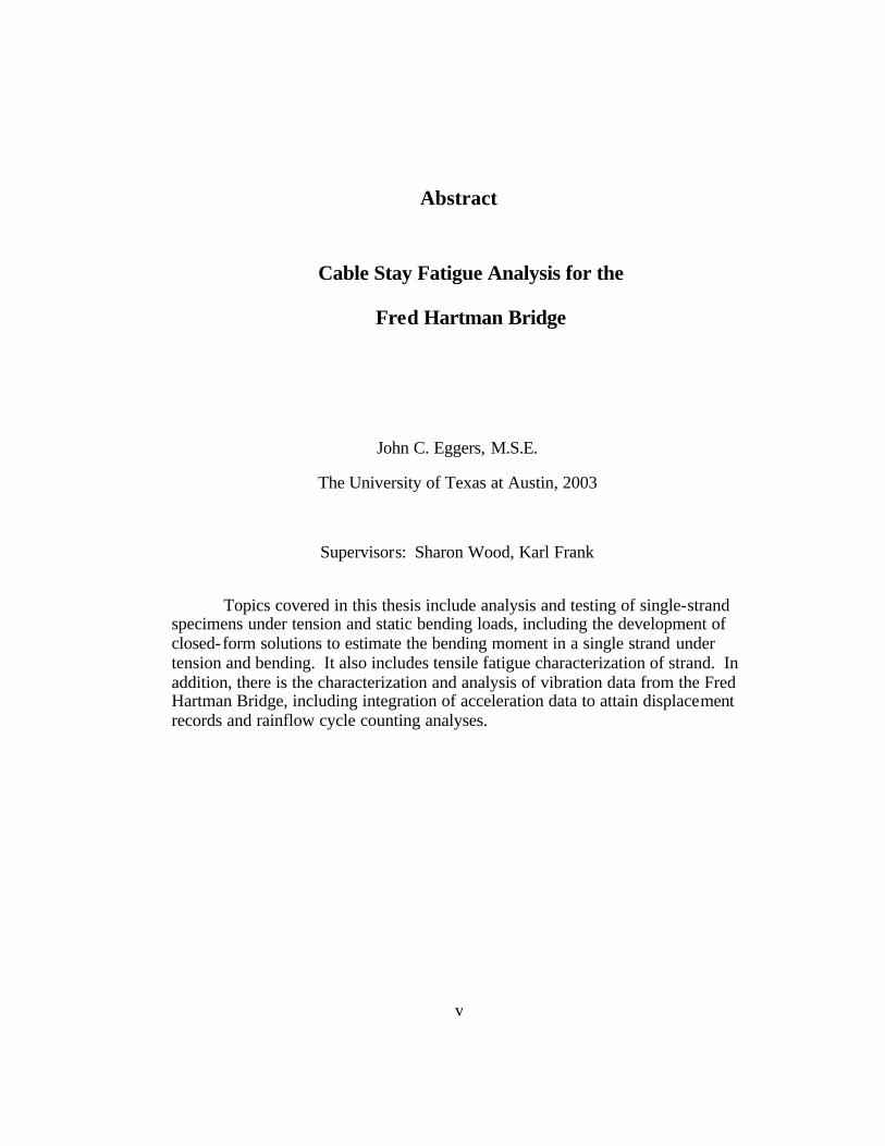
1.3.2 Full-Scale Bending Fatigue Testing
As of May 2003, five full-size cable stay fatigue tests have been
completed. Each test specimen was constructed similar to the smallest stay cable
on the bridge, and the length of each specimen was approximately 33 ft. For each
test, parameters such as the grout mix design, transverse displacement amplitude,
and other construction variables were varied. An overview of the 5 full-sized
tests is shown in Table 1.1. The 2001 thesis by Poser documents the behavior of
the first two specimens.
Table 1.1Full-Sized Specimen Test Summary
Specimen Displacement Testing Total NumberNo. Amplitude (+/- in.) Frequency (Hz) of Cycles1 1.60 0.9 2,808,3982 1.60 0.7 2,865,1033 1.60 2.2 4,961,5604 1.10 3.0 8,775,2455* 1.60 3.0 5,211,056
* Specimen 5 was ungrouted and there were no wire failures

7
1.3.3 Computational Models
Previously on this project, Dowd (2001) developed a finite element model
(FEM) of the full-scale strand specimen using beam elements and transformed
sections. Comparison of the FEM model and the results of the full-scale test
described above indicated that the FEM model overestimates the cable stiffness
by nearly a factor of 2. Further refinement of the FEM model is needed to
develop a more realistic model of the test specimens.
1.4 TOPICS COVERED IN THIS THESIS
This thesis describes research activities related to three different
components of the UT research project. While this thesis does not discuss the
results of the full-scale tests or the development of the computational models
specifically, it does describe research related to the research at UT. Topics
covered in this thesis include analysis and testing of single-strand specimens
under tension and static bending loads, tensile fatigue characterization of strand
used to construct full-scale specimens 1 through 6, and characterization and
analysis of vibration data from the Fred Hartman Bridge.
1.4.1 Single Strand Bending Tests
Chapter 2 of this thesis describes the testing of three single-strand
specimens under tension and static bending and the development of closed-form
solutions. The closed-form solutions are intended to bound the stiffness of the
single-strand specimens and are used to estimate the moment in the strand.
Comparisons are made between the closed-form solutions, single-strand results,
and the results of the full-scale specimens.
An estimate of the single-strand stiffness is developed based on the
closed-form solution, using an effective moment of inertia and modulus (effective

8
EI). The results from this phase of the research will be used by the research team
to refine the computational models.
1.4.2 Fatigue Tests of Strand in Tension
Tension fatigue tests were used to establish the fatigue characteristics of
the strand used to construct the first six, 19-strand stay cable specimens. Chapter
3 describes the testing procedure, presents the results, and compares the results
with specified design criteria and othe r published strand fatigue data. The results
of the strand fatigue tests will be used by the research team to characterize the
axial fatigue performance of the strand.
1.4.3 Characterization of Cable Vibration Data from the Fred Hartman
Bridge
Data from JHU is used to characterize the cable motions in Chapter 4 of
this thesis. Acceleration data from wind-rain vibration events are used to
calculate the displacement history during ten different wind-rain events. The
displacement histories are used to characterize the vibration of the cables in terms
of Lissajous diagrams and mode number.
The displacement histories for each cable are characterized using rainflow
counting and the results are used to develop an equivalent displacement for each
cable. Next, statistical data compiled by researchers at JHU are used to estimate
the amount of time that each of the cables has experienced wind-rain induced
vibrations. These results are compared with the observed fatigue life of the first
five stay cable specimens.
The result s of the vibration characterization are in the form of an
equivalent displacement at the location of the accelerometer and an estimated
number of cycles that the cable has experienced since construction. After
refinement of the computational model, the research team should be able to use

9
the results of the cable fatigue characterization and the cable stay tests to estimate
fatigue damage and the remaining life of the stay cables that support the Fred
Hartman Bridge.

10
CHAPTER 2
Single-strand Bending Tests
This chapter explains the development of simplified closed-form solutions
for single-strand bending and describes the testing of single 0.6- in., 7-wire strand
under tension and bending.
2.1 INTRODUCTION
Analysis of stay cables under tension and bending loads is a complex
problem. The interactions between the grout and strands and the relative
movement of the wires within each strand are not fully understood. Previously on
this project, analysis and testing of full-scale cable specimens was performed
(Dowd 2001, Poser 2001). The full-scale specimens were 19-strand cables, 33
feet in length and similar in design to cables constructed on the Fred Hartman
Bridge. Each was pre-stressed to 40 percent of the guaranteed ultimate strength
and bending was induced by imposing a mid-span deflection.
Dowd (2001) developed a finite element model of the full-scale strand
specimen using beam elements and transformed sections. Table 2.1 shows a
comparison of the transverse load calculated using that FEM model for a mid-
span deflection of 1.6 in. (Dowd 2001) and the measured transverse load for
specimens one and two for a mid-span deflection of 1.6 in. (Poser 2001).

11
Table 2.1 Difference between FEM and Measured Response
FEM Measured* DifferencePrestress Force (kip): 445 445 -
Mid-span Deflection (+/- in.): 1.6 1.6 -Transverse Force (+/- kip): 16.0 7.6 8.4
*Measured values are identical for both specimen 1 and specimen 2
As shown in Table 2.1, the transverse load estimate from the FEM
analysis overestimates the measured transverse load by more than a factor of 2.
Further refinement of the FEM model is needed to develop a more realistic model
of the test specimens. In order to understand the response of the cable, attempts
were made to measure the strain in the strand at various locations in the grouted
specimen. Unfortunately, it was difficult to obtain useful strain data. Grouting
and stressing the strand damaged the strain gages attached to the strand and the
research team was unable to find an appropriate adhesive for attaching the strain
gages to the polyethylene pipe.
Because of the difficulties encountered in measuring the strain response of
the grouted, 19-strand specimens, tests of an ungrouted, single-strand specimen
were planned. The results of these tests should assist the development of a
refined FEM model for the grouted 19-strand specimen. For comparison, closed-
form solutions were also developed for a single strand under tension and bending.
2.2 CLOSED-FORM SOLUTIONS
Two closed-form solutions were developed for a single strand subjected to
tension and bending due to lateral loading. In the first solution, a simply-
supported beam with axial tension was subjected to a transverse load at mid-span.
In the second, the ends of the beam were assumed to be fixed against rotation.
12
The two solutions represent lower and upper bounds for the stiffness of a single
strand.
The simply-supported solution is meant to be the lower bound for the
stiffness because the strand has some rotational restraint at the ends due to the
face of the chucks bearing on the test frame. Note that the simply-supported
solution has no reaction moment.
The fixed end beam solution is meant to be the upper bound solution for
two reasons. First, it is believed that the ends of the strand are only partially
restrained against rotation. Second, the EI used in the fixed end beam solution
assumes a solid beam cross section but the strand is composed of seven separate
wires. These wires can slip relative to each other unlike a solid cross section,
resulting in a response that is less stiff than the fixed end solution (Papaoliou,
1999). Note that because the fixed end solution does have reaction moments, the
moment diagram near the supports should also be an upper bound solution for the
moment in the strand.
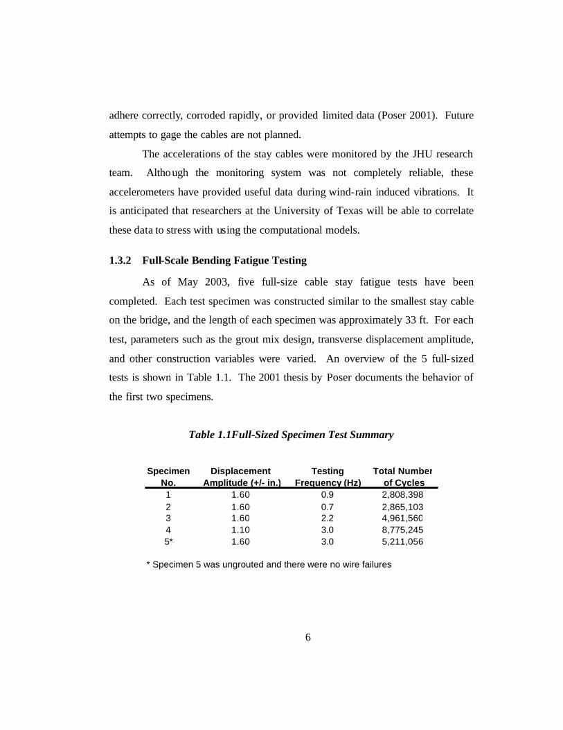
The derivation of both closed-form solutions assumes the same basic
parameters. First, the strand is viewed as a tens ion strut with a transverse force at
mid-span (Fig. 2.1). Second, to include secondary bending effects due to the
tension in the strand, the free-body diagram (FBD) includes an initial deflection
due to the transverse load (Fig. 2.2). This is similar to the derivation of a
compression member with secondary bending (i.e. Euler buckling), except the
solution is stable due to the tension in the strand. Deformation due to shear was
ignored due to the large span-to-depth ratio of the strand. Because the transverse
load is located at mid-span, the solutions are symmetric. Therefore the solutions
are derived for only half of the beam, and 2/0 Lx ≤≤ .
13
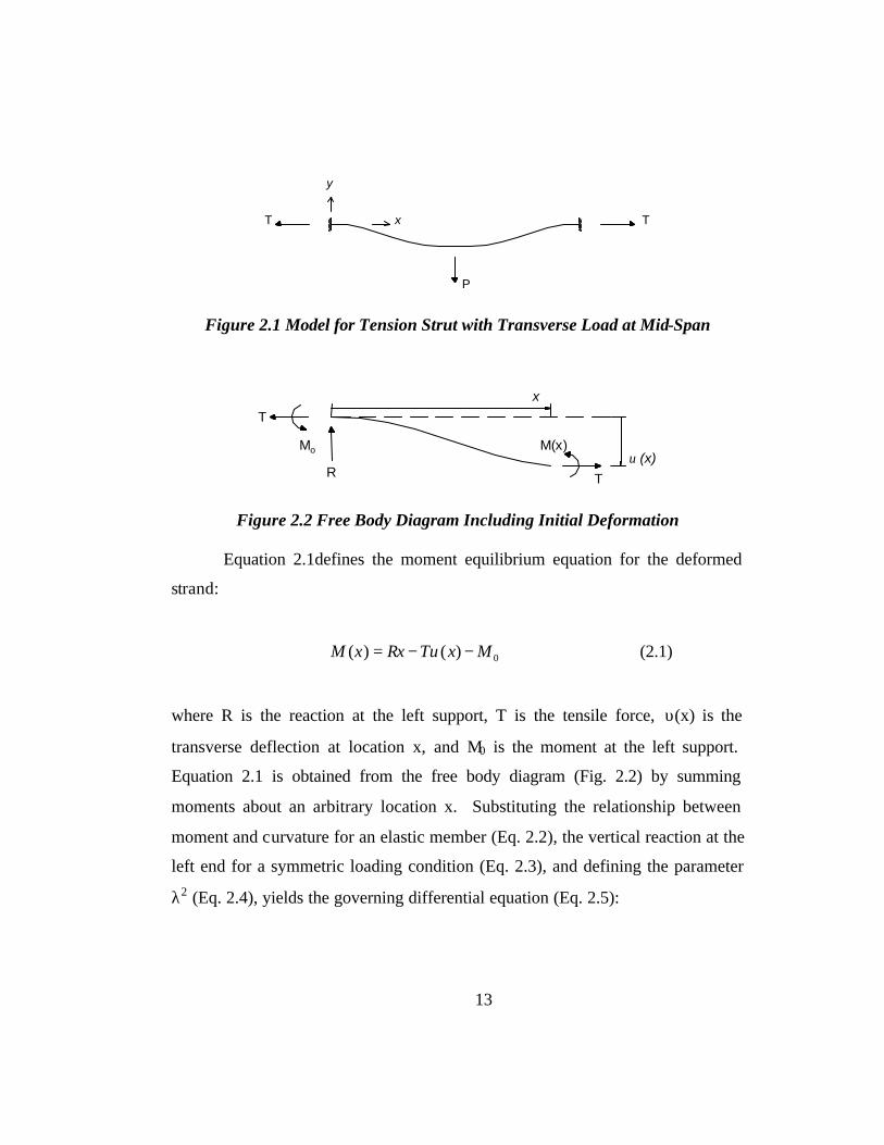
Figure 2.1 Model for Tension Strut with Transverse Load at Mid-Span
Figure 2.2 Free Body Diagram Including Initial Deformation
Equation 2.1defines the moment equilibrium equation for the deformed
strand:
0)()( MxTRxxM −−= υ (2.1)
where R is the reaction at the left support, T is the tensile force, υ(x) is the
transverse deflection at location x, and M0 is the moment at the left support.
Equation 2.1 is obtained from the free body diagram (Fig. 2.2) by summing
moments about an arbitrary location x. Substituting the relationship between
moment and curvature for an elastic member (Eq. 2.2), the vertical reaction at the
left end for a symmetric loading condition (Eq. 2.3), and defining the parameter
λ2 (Eq. 2.4), yields the governing differential equation (Eq. 2.5):
T T
P
x
y
T
TR
Mo M(x)
x
υ (x)
14
2
2 )()(
dxxd
EIxMυ
−= (2.2)
2P
R = (2.3)
EIT
=2λ (2.4)
EIM
xEIP
xdx
xd 022
2
2)(
)(+
−=− υλ
υ (2.5)
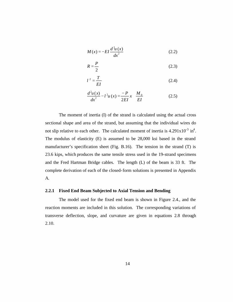
The moment of inertia (I) of the strand is calculated using the actual cross
sectional shape and area of the strand, but assuming that the individual wires do
not slip relative to each other. The calculated moment of inertia is 4.291x10⁻³ in4.
The modulus of elasticity (E) is assumed to be 28,000 ksi based in the strand
manufacturer’s specification sheet (Fig. B.16). The tension in the strand (T) is
23.6 kips, which produces the same tensile stress used in the 19-strand specimens
and the Fred Hartman Bridge cables. The length (L) of the beam is 33 ft. The
complete derivation of each of the closed-form solutions is presented in Appendix
A.
2.2.1 Fixed End Beam Subjected to Axial Tension and Bending
The model used for the fixed end beam is shown in Figure 2.4., and the
reaction moments are included in this solution. The corresponding variations of
transverse deflection, slope, and curvature are given in equations 2.8 through
2.10.

15
Figure 2.3 Model for Fixed End Beam
T
Mx
TP
xT
Mx
TP
x 00
2)cosh()sinh(
2)( −++
−= λλ
λυ (2.5)
TP
xT
Mx
TP
xdxd
2)sinh()cosh(
2)( 0 ++
−= λλυ (2.6)
)cosh()sinh(2
)( 02
2
xT
Mx
TP
xdxd
λλλυ +−
= (2.7)
The transverse stiffness corresponding to this model with a tension force
of 23.6 kip is 257 lb/in. The maximum moment for the fixed end beam, which
occurs at the ends, is 586 lb- in. for a transverse load of 514 lb. Figure 2.5 shows
the moment for the first 12 in. of the fixed end solution. Note that the moment is
essentially zero at 12 in. from the face of the chuck. The deflected shape and
moment diagrams for the fixed end beam solution are plotted for a mid-span
deflection of 2.0 in. are in Appendix A.
T T
P
x
y

16
-600
-550
-500
-450
-400
-350
-300
-250
-200
-150
-100
-50
00 1 2 3 4 5 6 7 8 9 10 11 12
Length from Face of Chuck (in.)
Mo
men
t (ki
p-i
n.)
Figure 2.4 Moment Diagram for Fixed end Beam
2.2.2 Simply-Supported Beam Subjected to Axial Tension and Bending
The model used for the simply-supported beam is shown in Figure 2.3,
and the reaction moments are zero. The corresponding variations of transverse
deflection, slope, and curvature are given in equations 2.5 through 2.7. Although
presented in a different form, the results are identical to those given by
Timoshenko (1956). Note that equations 2.8 through 2.10 are identical to
equations 2.5 through 2.7 with the exception that the end moment, M0, is equal to
zero for the simply-supported beam.

17
Figure 2.5 Model for Simply-Supported Beam
xTP
Lx
TP
x2)2/cosh(
)sinh(2
)( +−
=λ
λλ
υ (2.8)
TP
Lx
TP
xdxd
2)2/cosh()cosh(
2)( +
−=
λλ
υ (2.9)
)2/cosh(
)sinh(2
)(2
2
Lx
TP
xdxd
λλλ
υ−
= (2.10)
The transverse stiffness corresponding to a model with a tensile force of
23.6 kip is 241 lb/in., where transverse bending stiffness is defined as P divided
by mid-span deflection. The deflected shape and moment diagram for the simply-
supported solution are plotted for a mid-span deflection of 2.0 in. are in Appendix
A. The simply-supported solution provides a lower bound for the transverse
bending stiffness of the single-strand. The maximum moment for the simply-
supported beam, which occurs at the mid-point, is 549 lb- in. for a transverse load
of 482 lb. Because the end moments are zero, the moment diagram represents the
upper bound for the moment at mid-span of the strand.
2.3 SINGLE-STRAND TESTS
Static load tests were performed on single-strands and then compared with
the results of the closed-form solutions. The tests were comprised of a single-
strand under tension with an applied load at mid-span.
T T
P
x
y

18
2.3.1 Test Apparatus
The test frames used for the single-strand tests were the same frames used
for the full-scale, bending fatigue tests (Poser 2001). Test frames consisting of
two longitudinal wide flange columns and built up crossbeams at both ends were
used to react the initial stressing force and the forces from the single-strand test.
Two longitudinal W14x90 columns serve as axial compression members to
provide reaction to the prestress force in the strand (Fig. 2.6). The built up
crossbeams at both ends consist of two W18x97 beams with welded stiffeners and
a load distribution plate with an opening for the strand. The load distribution plate
is in direct contact with the strand chuck and directs the forces from the strand
into the test frame (Fig. 2.7). To provide reaction to the vertical shear forces the
frame was anchored to the laboratory floor.
For each test, a chain hoist hanging from an overhead arm was attached to
the strand and used to impose deformations at mid-span of the strand (Figure 2.6).
The magnitude of the tensile load in the strand and the applied transverse load
were measured using load cells. The mid-span deflection was measured using a
linear potentiometer. In addition, strain gages were attached to individual wires
of the strand near the face of the chuck at the dead end of the specimen.

19
Figure 2.6 Test Frame with Specimen Installed
For each test, a single 0.6 in., 270 ksi, 7-wire strand was placed in the test
frame. The strand was then tensioned to approximately 23.6 kips which is 40% of
the guaranteed ultimate tensile strength, the same stress used for the full-sized
specimens and the Fred Hartman Bridge stay cables. The area of the strand used
to calculate the stress was 0.2185 in. and this area was verified by UT researchers
(Fig. B.17). Stressing was performed using a single-strand hydraulic ram and
held in place with reusable chucks (Fig. 2.7). The total length of each specimen
was 33 feet, which was measured from the inside face of chuck to the inside face
of chuck. The transverse displacement at mid-span was increased from 0 to 2 in.
in increments of approximately 0.1 in. during each test. All loads were applied
statically.
Strand
Longitudinal Beams
20
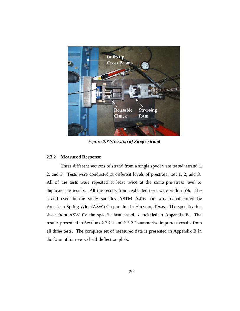
Figure 2.7 Stressing of Single-strand
2.3.2 Measured Response
Three different sections of strand from a single spool were tested: strand 1,
2, and 3. Tests were conducted at different levels of prestress: test 1, 2, and 3.
All of the tests were repeated at least twice at the same pre-stress level to
duplicate the results. All the results from replicated tests were within 5%. The
strand used in the study satisfies ASTM A416 and was manufactured by
American Spring Wire (ASW) Corporation in Houston, Texas. The specification
sheet from ASW for the specific heat tested is included in Appendix B. The
results presented in Sections 2.3.2.1 and 2.3.2.2 summarize important results from
all three tests. The complete set of measured data is presented in Appendix B in
the form of transverse load-deflection plots.
Reusable Chuck
Stressing Ram
Built-Up Cross Beams

21
2.3.2.1 Strand Stiffness
The single-strand tests included static tests at values of axial prestress
ranging from 7.5 kips to 30.8 kips. The observed stiffness of the strand increased
nearly linearly with prestress force as seen in Figure 2.8. Because of the
inaccuracies in the stressing equipment, it was difficult to stress the strand to the
desired level so a least-squares approach was used to relate the observed stiffness
to the applied prestress force (Fig. 2.8). The resulting least-squares linear
approximation is shown in Equation 2.11. The corresponding R2 value is 0.99.
Based on these results, the average stiffness of the strand with an axial tension of
23.6 kip was 251 lb/in.
0
50
100
150
200
250
300
350
0 5 10 15 20 25 30 35
Tension (kip)
Stif
fnes
s (lb
/in)
Figure 2.8 Stiffness vs. Prestress Force

22
max
86.35.10υ
PTk =+= (2.11)
Where k is the transverse stiffness of the strand and T is the initial
prestress axial force.
The measured stiffness of the single-strand is compared with the measured
stiffness of cable stay specimens 1 through 5 in Table 2.2. For comparison the
equivalent stiffness per strand is calculated as the measured stiffness of the
specimen divided by the number of strands in that specimen. Note that the
prestress tension is 108 ksi, 23.6 kip/strand, for all the specimens in Table 2.2.
The information about the ungrouted specimen is from cable stay specimen 5,
which was constructed and tested in early 2003.
Table 2.2 Measured Stiffness of Various Specimens
Measured Number of Stiffness/Strand Difference fromGrouted/Ungrouted Stiffness (lb/in.) Strands (lb/in.) Single Strand (%)
Single Strand: Ungrouted 251 1 251 -Cable Stay 1*: Grouted 4750 19 250 -0.4%Cable Stay 2*: Grouted 4750 19 250 -0.4%Cable Stay 3: Grouted 4685 19 247 -1.8%Cable Stay 4: Grouted 4535 19 239 -4.9%Cable Stay 5: Ungrouted 4083 19 215 -14.4%
* (Poser 2001)
The effective stiffness per strand is essentially the same for the four
grouted specimens and the single-strand in Table 2.2. The full-scale ungrouted
specimen (Cable Stay 5) had the largest difference from the single-strand results.
The reason for this is unknown and further investigation needs to be performed to
identify the cause of this apparent difference.
Note that the measured lateral bending stiffness of the strand was
dependent on the amplitude of the lateral deformation. Data are plotted in Figure
2.9 for one loading and unloading cycle. This trend was observed with all the

23
single-strand tests. The stiffness increases slightly with deflection due to
lengthening of the cable and hence increasing its tension (Fig. 2.10). This
increase in axial tension due to lengthening was not included in the closed-form
solutions. Because the increase in stiffness was approximately 2%, it was
considered to be insignificant. The average stiffness is used in all comparisons.
Also, all the tests indicated a reduction in stiffness of between 2% and 5%
after the first cycle of deflection (Fig. 2.9). However, the amplitude of the
variation decreased after repeated cycles. This may be due to additional seating
of the wedges during the first few cycles of each test.
232
233
234
235
236
237
238
239
240
241
242
0.0 0.5 1.0 1.5 2.0 2.5
Defection (in.)
Stif
fnes
s (lb
/in)
Figure 2.9 Stiffness vs. Deflection of Single-strand for a
Prestress Force of 23.3 kip
Loading
Unloading

24
23.10
23.15
23.20
23.25
23.30
23.35
23.40
23.45
23.50
0.0 0.5 1.0 1.5 2.0 2.5
Defection (in)
Stif
fnes
s (k
ip/in
)
Figure 2.10 Tensile Load vs. Deflection of Single-strand for a
Prestress Force of 23.3 kip
2.3.2.2 Strand Strain
Two sets of strain gages were attached to the individual wires of the strand
located near the face of the chuck at the dead end of the specimen. The gage
location closest to the chuck was labeled location A and the location further from
the chuck was labeled location B (Figure 2.11). The distances shown in Figure
2.10 were measured during Test 2 and Test 3 for Strand 3. The actual location of
each gage was determined after each test by measuring the distance from the gage
to the teeth marks corresponding to the first wedge.
Figure 2.11 Location of Strain Gages for Strand 3,
Test 2 and 3

25
Note that the strain data from the tests of strand 3 represent the most
complete set of data. For various reasons many of the strain gages from tests of
strand 1 and 2 were damaged or not functioning correctly. For this reason, only
the data from strand 3 will be discussed in this section. Note that the strain data
from the other tests are plotted in Appendix B. All the strains discussed in this
section represent the change in strain due to bending; only initial strains due to the
prestress force are not included. Note that the strains due to prestress from each
of the gages were within 5% for each test.
Strain gages were placed on each of the outer 6 wires to monitor the
response of the strand during bending. Figure 2.12 shows the variation of strain
with mid-span deflection for a strand with a prestress force of 23.5 kip. The data
are plotted such that increases in strain due to tension are positive.
-400
-300
-200
-100
0
100
200
300
400
0.00 0.50 1.00 1.50 2.00 2.50
Deflection (in.)
Str
ain
(10
-6) A1
A2A3A5
A6
Figure 2.12 Strain Measured at Location A, Strand 3, Test 2
As expected, the strain gages attached to the extreme top and bottom wires
experienced the highest absolute strains. Gages A1 and A5 were the furthest from
the center of the cross section (Fig. 2.13). Note that the exact location of the

26
gages relative to the cross section was difficult to determine because the cross
beams at the end of the frame prevented direct observation (Figure 2.7).
A1A2
A3
A4
A6
A5
A1A2
A3
A4
A6
A5
Figure 2.13 Approximate Location of Strain Gages at Location A
for Strand 3, Test 2
It is important to note that the maximum strain measured by gage A1 is
higher than the maximum strain measured by gage A5. This is because gage A1
was located almost directly below the centroid of the strand, while gage A5 was
slightly off center of the centroidal axis. In addition, the strains are affected by
the increase in tension during each test, so the measured strains are slightly higher
than the actual bending strains. Similarly to the other tests, at least one of the
strain gages did not adhere properly to the strand and data are not available for
strain gage A4.
The data recorded at location B during the same loading cycle are plotted
in Figure 2.14. The tensile strains increased in all gages at location B, although
the magnitude of the variation was significantly less than that measured at
location A. In tests of strands 1 and 2, it was shown that the bending strain in the
strand is essentially zero approximately 12 in. from the face of the chuck, which
agrees with the closed-form solution for a fixed end beam.

27
0
10
20
30
40
50
60
70
80
90
100
0.00 0.50 1.00 1.50 2.00 2.50
Deflection (in.)
Str
ain
(10
-6) B1
B2
B3B4
B5
Figure 2.14 Strain Measured at Location B, Strand 3, Test 2
An interesting event that occurred frequently during the single-strand tests
was that the measured strain did not return to zero after unloading of the
specimen. The result is an apparent residual strain. Figure 2.15 shows one such
example. Note that the apparent residual strain appeared for three of the five
strain gages. The maximum residual strain in this example was 77 microstrain
and occurred on strain gage A5. Possible sources are mechanics of the strand
during bending or partial release of the strain gages, but the reason for the
apparent residual strain was not positively identified.

28
-200
-100
0
100
200
300
400
0 0.5 1 1.5 2 2.5
Deflection (in.)
Str
ain
(10-
6)A1
A2
A3
A5
A6
Figure 2.15 Strain Measured at Location A, Strand 1, Test 1
Showing Residual Strain
2.4 COMPARISON OF M EASURED AND CALCULATED RESPONSE
The measured response of the strands are compared with the expected
response calculated using the closed-form solutions in this section. Two types of
comparisons are discussed: stiffness of the strand and moments inferred from the
measured strains. The stiffness from the closed-form solutions corresponds to an
initial axial tension of 23.6 kip. In addition, the moment of inertia used in the
closed-form solution corresponds to a solid section of the same area and shape as
the 7-wire strand.
2.4.1 Stiffness Comparison
The average measured stiffness is compared with the stiffness calculated
using the closed-form solutions in Table 2.3. As expected, the closed-form
solutions bound the measured response of the strand. As stated earlier, the
average measured stiffness of the strand is based on a linear least-squares
approximation of measured data for six values of axial tension between 7.5 and
30.8 kip (Fig. 2.8).

29
Table 2.3 Stiffnesses of Closed-form Solution and Measured Response
with a Prestress of 23.6 kip
Stiffness (lb/in.)Tests: 251 -
Simply-Supported: 241 -4.0%Fixed End Solution: 257 2.4%
Difference from Measured Stiffness (%)
The actual moment of inertia of the strand is expected to be less than the
moment of inertia of a solid section because the individual wires of a strand slip
relative to each other as the load is applied. While it was not possible to measure
the slip between wires, the effective EI of the strand can be estimated from the
fixed end solution such that the measured and calculated strand stiffnesses are
equal. Figure 2.16 shows the load-deflection curve for the fixed end solution and
the measured response of a strand with a prestress force of 23.5 kip. Note that
23.5 kip was the closest to the desired level of 23.6 kip obtained during the single-
strand tests. The fixed end solution is linear and can be described with Equation
2.13.
max8.256 υ=P (2.13)
where P is the transverse load and υmax is the mid-span deflection. Note that the
measured response is less stiff than the fixed end solution. This implies that wire
slip did influence the bending response of the single strand.

30
0
100
200
300
400
500
600
0.0 0.5 1.0 1.5 2.0 2.5
Strand Deflection at Mid-Point (in.)
Lo
ad a
t Mid
-Po
int o
f Str
and
(lb
)
F-F Solution
Measured
Figure 2.16 Comparison of Load-Deflection Curves for Test 2 of Strand 3 and
the Fixed End Solution
The difference in stiffness between the fixed end beam solution and the
measured results for test 2 of strand 3 is approximately 6%. In order for the
observed response to match the fixed end solution an effective EI of 0.94EI
should be used. Note that this effective EI is based on only one test.
An interesting thing to note is that the comparisons presented in this
section are only applicable to single-strand bending. It is unknown how these
results relate to the larger 19-strand tests. With the increased section size, the
amount of wire slip could be significantly different. It is recommended that
further testing be performed on multiple-strand specimens, with less than 19
strands, to define the relationship between the single-strand and 19-strand
specimens.

31
2.4.2 Moment Comparison
Before the moments from the closed-form solutions can be compared with
the measured data, moments must be calculated from the measured strain. The
following assumptions were made to estimate moments from the strain data:
o The cross section of the strand is idealized as three separate layers and
slip is ignored within each layer (Figure 2.17).
o The strain profile within each layer is assumed to be constant;
however, the strains in adjacent layers are not equal.
o The strains in the top and bottom layers are assumed to be the
maximum measured strains. The strain in the middle layer is
calculated to satisfy equilibrium within the cross section.
o The longitudinal stress in the strand is related to the measured strain in
the wires using Equation 2.13:
)cos(φεσ E= (2.13)
where σ is the effective longitudinal stress in the strand, φ is the
orientation of the wires relative to the longitudinal axis of the strand
(approximately 9°), ε is measured strain in the wires oriented along the
axis of the wires, and E corresponds to the effective longitudinal
modulus of the strand (28,000 ksi).

32
Figure 2.17 Cross-section Stress Diagram for a Single-Strand in Bending
(ignoring prestress)
Moments were calculated at location A. During cycles 1 and 2 location A
was approximately 2.5 in. from the face of the chuck. During cycles 3 and 4
location A was approximately 1.8 in. from the face of the chuck. The calculated
moments are summarized in Table 2.4 and are compared with the moments
calculated using the closed form solutions for the fixed end beam. The strains
used to calculate the moments in Table 2.4 were obtained during a mid-span
deflection of 2.0 in. The moments in the simply-supported beam are essentially
zero near the ends, so these results are not included in the summary.
Table 2.4 Estimated Moments in Strand 3, Test 2
Compared with Closed-form Solution
Distance from Moment DifferenceChuck (in.) (lb-in) (%)
Fixed-Fixed Solution: 1.8 271 -Fixed-Fixed Solution: 2.5 204 -
Test 2, Cycle 1: 2.5 196 4%Test 2, Cycle 2: 2.5 200 2%Test 2, Cycle 1: 1.8 241 11%Test 2, Cycle 2: 1.8 241 11%
The moments calculated using the closed-form solution exceeded the
moments inferred from the measured strains. Note that as the distance from the

33
face of the chuck increases, the difference between the moment and the fixed end
solution decreases. One reason for this correlation is that slip between the wire
layers increases with additional curvature. The relationship between the wire slip
and curvature may be empirically estimated with more testing performed at other
distances from the chuck. The empirical relationship between wire slip and
curvature may be better understood with additional tests with multiple strands as
discussed in Section 2.4.1.
2.5 SUMMARY
This chapter explains the development of closed-form solutions for a
single 7-wire strand under tension and bending. In addition, closed-form
solutions for a beam under tension and bending are used to bound the results of
the tests. Based on the results, the following conclusions were made:
o The single-strand tests indicated that the strain due to bending is
essentially zero at a distance of 12 in. from the face of the chuck,
which agrees with the FEM model developed by Dowd (2001).
o When comparing the estimated average stiffness of the single-strand
specimens, it was noted that the single-strand is approximately 2% less
stiff than a fixed end classical model and approximately 4% more stiff
than the simply-supported classical model. This concludes that the
two models are upper and lower bounds to the actual stiffness of the
strand.
o When comparing the fixed end beam solution to the results of test 2
from strand specimen 3, it was found that the fixed end solution was
stiffer than the response of the strand. The difference in stiffness at
2.0 in. of deflection was approximately 6%. An effective EI of 0.94 EI

34
can be used to predict the response of a single strand using the fixed
end beam solution. In addition, it was noted that the relation between
the single-strand response and the 19-strand response is unknown with
respect to wire slip.
o Based on the moment comparison between the single-strand tests and
the closed-form solutions, it appears that the actual moment in the
strand is between 2% and 9% less than the fixed end closed form
solution. This indicates that the fixed end solution can be used for an
adequate approximation of the single-strand specimens since the
simply-supported solution has an end moment of zero.

35
CHAPTER 3
Strand Tension Fatigue Test
3.1 INTRODUCTION
Tension fatigue tests were conducted to establish the fatigue
characteristics of the strand used to construct the first six, 19-strand stay cable
specimens. This chapter describes the testing procedure, presents the results, and
compares the results with specified design criteria and other published strand
fatigue data. The results of the strand fatigue tests will be used by the research
team to interpret the fatigue response of the stay-cable specimens. Specifically,
the results will be used to determine if bending of the stay-cable specimens causes
a reduction of fatigue life due to fretting or another mechanical interaction.
3.2 TEST PROGRAM
A total of twelve strand specimens were subjected to tensile fatigue
loading. Each test was performed with an average stress of 104 ksi, the same
tension as the prestress tension used in the bending fatigue tests. Stress ranges for
the individual tests were 20, 30, and 40 ksi. The test specimens were subjected to
cyclic loads with the prescribed stress range until at least one wire fractured or the
number of cycles exceeded 6,000,000. Data from eight fatigue tests are used to
evaluate the strand. Of the remaining four specimens, three tests ended
prematurely when the strand failed within the grips and one specimen was
inadvertently loaded to more than 95% of the guaranteed ultimate tensile strength
before the fatigue loads were applied. The data from these tests are presented for
completeness, but are not used to evaluate the strand.
36
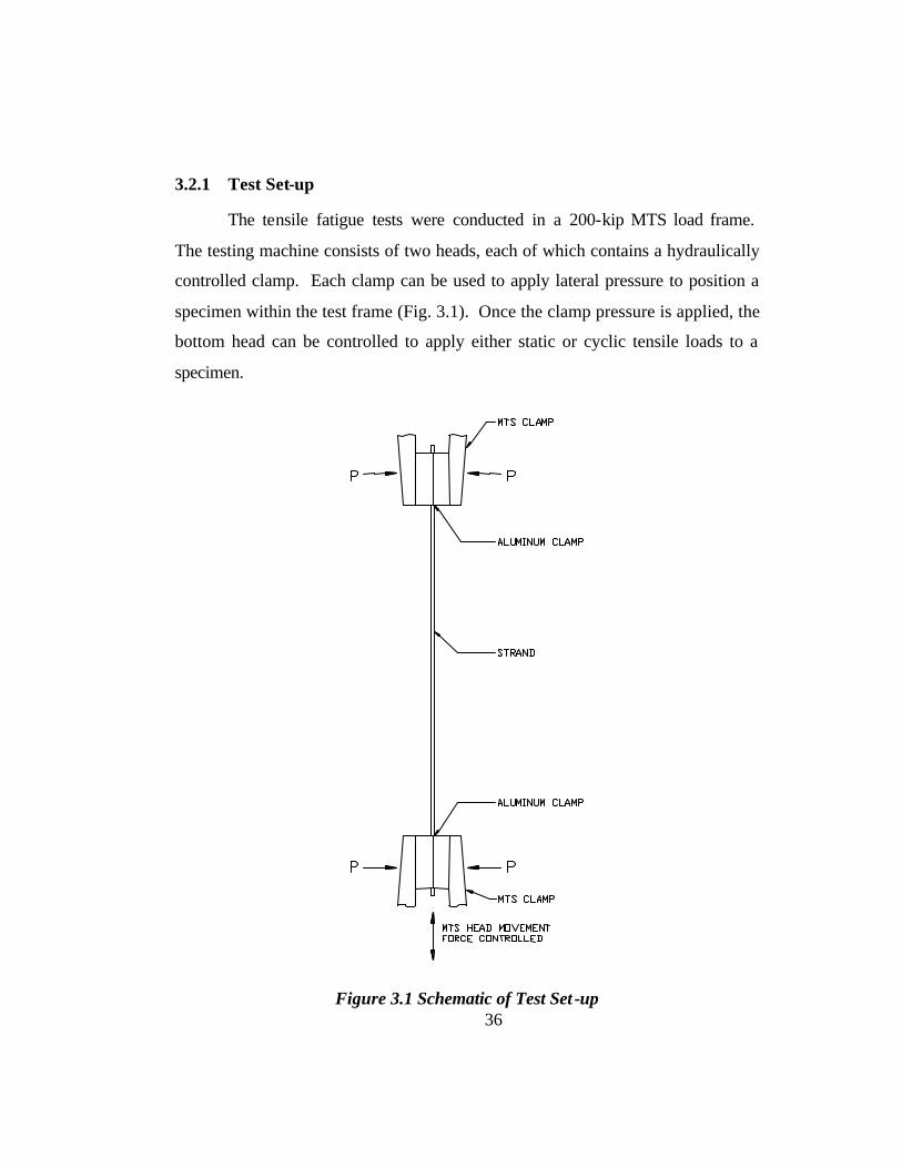
3.2.1 Test Set-up
The tensile fatigue tests were conducted in a 200-kip MTS load frame.
The testing machine consists of two heads, each of which contains a hydraulically
controlled clamp. Each clamp can be used to apply lateral pressure to position a
specimen within the test frame (Fig. 3.1). Once the clamp pressure is applied, the
bottom head can be controlled to apply either static or cyclic tensile loads to a
specimen.
Figure 3.1 Schematic of Test Set -up

37
The cyclic loading was controlled using PC-based software developed by
MTS (Test Star II). The load for each of the tests was applied using a load-
controlled sine wave with feedback compensation. The feedback compensation
corrects for errors between the input function and the actual motion of the test
frame. The frequency of the load is also controlled by the software. In each test,
the highest testing frequency possible was used. This frequency was limited by
degradation of the sine wave function or inducing excessive dynamic motions in
the test frame. Frequencies for the tests were between 1.5 and 4 Hz.
Each strand specimen was approximately 48” long from face-of-clamp to
face-of-clamp. During installation special care was taken to position each
specimen in the test frame vertically to minimize eccentricity. A special clamp
system was developed so that the MTS grips could hold the strand without
crushing the specimen. The aluminum clamps are discussed in the following
section.
3.2.2 Aluminum Clamps
Aluminum clamps were built to hold the strand within the test machine
grips. The aluminum clamps were designed based on recommendations by Lamb
(1985). A general schematic of the clamp design is shown in Figure 3.2. Note
that the dimensions of the clamp may be adjusted for different sized strand. Also,
Lamb makes further recommendations to improve on the design shown below, but
those modifications were not made because the simple aluminum clamp system
worked well.

38
Figure 3.2 Schematic of Aluminum Clamp
The clamps were fabricated from a 5-in. long section of 2-in. square
aluminum bar. A ? ”-diameter hole was drilled longitudinally through the center
of the aluminum block. The hole was tapped approximately ? ” larger than the
hole, providing a rough surface with which to grip the strand. Additional smaller
holes are drilled near one end of the bar to hold the aluminum clamp on the strand
before grip pressure is applied. The bar is then cut in half along the longitudinal
axis (Fig. 3.2) and the strand is sandwiched between the two pieces of aluminum
(Figure 3.3).

39
Figure 3.3 Aluminum Clamp in Position on Strand
As seen in Figure 3.4, when the grip pressure is applied to the aluminum
clamps, the edges of the clamp come in contact with one another. The grip
pressure must be controlled so that the aluminum does not crush. Figure 3.5
shows the inside surface of a clamp after testing. Note that the threads in the
longitudinal hole allow the aluminum to conform to the shape of the strand. The
lower modulus of the aluminum compared with that of the steel reduces the stress
concentration at the clamp face which reduces the chance that a fatigue failure
will occur near the grips. An attempt was made to reuse the aluminum clamps for
more than one test, but the strand slipped through clamps that had been used
previously. The results presented in this chapter refer only to tests using new
aluminum clamps.

40
Figure 3.4 Aluminum Clamp under Pressure in MTS Grips
Figure 3.5 Photograph of Aluminum Clamp After Fatigue Test

41
3.3 RESULTS
The fatigue tests were performed at three different stress ranges: 20, 30,
and 40 ksi. The stress range and number of cycles for each test is shown in Table
3.1. As stated previously, four specimens failed prematurely (2, 5, 7, and 11).
The data from these tests are included in Table 3.1 for completeness, but are not
used to evaluate the strand. The area used to calculate the strand stress was
0.2185 in2 based on the manufacturer’s specification sheet (Fig. B.16). The strand
area was verified by researchers at UT (Fig. B.17).
Table 3.1 Single-strand Fatigue Test Results
Test No. Sr (ksi) N (cycles) Notes1 20 6,276,532 test stopped w/o failure2 40 187,873 Grip Failure3 40 365,3534 40 323,4695 40 145,098 Grip Failure6 30 3,301,9277 30 90,942 Accidentally loaded to 265 ksi before test8 30 1,009,6009 30 808,328
10 40 232,77311 40 142,987 Grip Failure12 30 848,521
The results from the tests are compared with three other established strand
fatigue standards: Paulson et al. (1983), PTI (1986), and PTI (2000). Tests
described in Paulson characterize the fatigue life of ½-in., 270 ksi, low-relaxation
strand. Paulson’s test procedures were nearly identical to those used in this thesis.
Paulson identified a mean fatigue life model (Eq. 3.1) and a lower bound
relationship (Eq. 3.2):

42
)(40.328.11)( rSLogNLog ⋅−= (3.1)
)(50.300.11)( rSLogNLog ⋅−= (3.2)
Where N is the number of cycles and Sr is the stress range in ksi.
The Post-Tensioning Institute (PTI) specifies a lower limit for fatigue life
for ASTM A416 uncoated, seven-wire, low-relaxation strand used to construct
stay cables (PTI 2001 and 1986). For comparison, the results of the tensile
fatigue tests are compared with the PTI specifications for 1986 and 2001. The
reason for providing both the 1986 and the 2001 PTI specifications is that there is
a significant difference between the fatigue requirements for the two editions. For
the same given minimum number of cycles, the 1986 PTI specification requires a
lower stress range than the requirements in the 2001 PTI specification. The 2001
stress ranges are between 14 and 16 percent higher than the 1986 stress ranges.
Another interesting note is that while fatigue requirements for individual strands
increased between the 1986 and 2001 specification, other related design limits did
not change. The maximum allowable stress range for assembled stay cables
remained unchanged and the assembled stay cable fatigue test stress range did not
change. It is the research team’s understanding that the 1986 PTI specification
was based on the results of Paulson’s data. The basis for the 2001 PTI strand
fatigue requirements is currently unknown.
Both PTI Specifications require that the maximum stress in each cycle be
0.45 f’ s (121.5 ksi), where f’s is the guaranteed ultimate tensile strength. In each
of the tests described in this report, the average stress was 0.4 f’s (108 ksi) and the
maximum stresses were 0.44 f’s, 0.46 f’s, and 0.47 f’s for the 20, 30, and 40 ksi
tests respectively. So the PTI test procedures and the test procedures used in this

43
thesis were nearly identical. The 1986 and 2001 PTI specification requirements
are summarized in Table 3.2.
Table 3.2 PTI Specification Strand Fatigue Requirements
2001 PTI Test 1986 PTI TestNo. of Cycles Stres Range (ksi) Stres Range (ksi) % Decrease
2,000,000 + 30.9 26.0 15.9%2,000,000 33.1 28.0 15.4%
500,000 43.8 37.5 14.4%100,000 64.3 55.0 14.5%
The test data are plotted in Figure 3.6. The lower bound and mean
relationship developed by Paulson and the PTI minimums are plotted. The
majority of the measured data fall between the mean and lower bound reported by
Paulson. This indicates that the strand had lower than average strength relative to
the sample population of strand that Paulson tested. In addition, the majority of
the tests also fell below the minimums set by the PTI specifications. It is
important to note that while only strand test number 1 satisfied the 2001 PTI
specification, strand test numbers 1 and 6 satisfied the 1986 specification. In
conclusion, the overall results indicate that the strand used in the full-sized
specimen tests have a lower than average fatigue life and do not satisfy either the
1986 or the 2001 PTI specifications.
It is recommended that further testing be performed on the strand to
construct the 19-strand specimens 1 through 6 to verify these results. In addition,
the PTI governing body should be contacted to verify the source of the 2001 PTI
strand fatigue requirements. If the 2001 fatigue requirements are correct, it may
be very difficult to obtain strand that satisfy the specification. It is also

44
recommended that strand used to construct future 19-strand specimens should be
tested in a similar manner and compared to the results presented in this thesis.
Single Strand Axial Fatigue Life
0
10
20
30
40
50
60
70
100000 1000000 10000000
Cycles
Str
ess
Ran
ge
(ksi
)
Test Data
Paulson Lower Limit
Paulson Mean Model
2001 PTI Lower Limit
1986 PTI Lower Limit
Eliminated Data
Figure 3.6 Tensile Fatigue Test Results
Note that Test 1 was stopped at 6,276,532 cycles without failure. This is indicated with
an arrow in Figure 3.6.
Test 6
Test 1

45
CHAPTER 4
Characterization of Cable
Vibration Data from the Fred
Hartman Bridge
4.1 INTRODUCTION
Researchers from Johns Hopkins University (JHU) instrumented the Fred
Hartman Bridge stay cables with accelerometers in October 1997. In this chapter,
the data from the accelerometers are used to characterize the motion of the stay
cables and estimate the number of wind-rain induced vibration cycles that each
cable has experienced since construction in September 1995.
The measured acceleration data are integrated numerically to calculate the
displacement response of each cable. Displacement histories are then used to
characterize the motion of the cables in terms of frequency, primary mode of
vibration, and maximum modal displacement. A rain-flow algorithm is then used
to count the number of displacement cycles experienced during each wind-rain
event.
The results of the rain-flow analyses are then used to develop an
equivalent displacement and calculate the average number of cycles per minute
for each cable. Next, the statistical data compiled by researchers at JHU are used
to estimate the amount of time that each of the cables has undergone wind-rain
induced vibrations. The estimated total number of cycles that each cable has
experienced is then compared with the observed fatigue life of the first five stay
cable specimens. After further cable stay testing, the research team should be
able to use the results of the cable fatigue characterization and the cable stay tests

46
to estimate fatigue damage and the remaining life of the stay cables that support
the Fred Hartman Bridge.
4.2 DATA
Researchers from JHU University instrumented and began collecting data
on the Fred Hartman Bridge in October 1997. Instrumentation includes 19 two-
axis accelerometers attached to the stay cables and a data acquisition system
(DAQ) with a sampling frequency of 40 Hz. The DAQ continually monitors each
transducer and saves the data to a disk whenever predetermined wind speed or
cable acceleration thresholds are exceeded. Each time the predetermined
thresholds are exceeded, the DAQ saves data for 5-minutes (Main et al. 2000).
Data received from JHU include a statistical database of all the records obtained
since instrumentation was installed and ten files, each with the acceleration
histories for seven different cables during wind-rain events. For each cable, the
acceleration history includes acceleration in two perpendicular planes.
4.2.1 Statistical Database
Researchers at JHU compiled a database of statistical information for each
5-minute record obtained since the Fred Hartman Bridge was instrumented in
October of 1997. Each record was divided into one-minute segments and
statistical data were calculated for each segment. This database is used to estimate
the number of times each cable experienced wind-rain induced vibration. The
following statistics were compiled for each one-minute segment:
o Maximum displacement (measured and modal)
o Primary vibration modes
o Rainfall and rate of rainfall during event
o Wind speed and direction
o Date and time of each record

47
o Other information not applicable to this report
Note that the DAQ system thresholds were set so that all the vibration
events that occurred while rain was falling were recorded. The vast majority of
the recordings are not large amplitude events such as wind-rain events, but are
small amplitude events. For this reason, wind-rain induced vibrations must be
identified within the database using some statistical criteria. The statistical
criteria used here is maximum displacement. The displacement criteria and the
development of the criteria are discussed in Section 4.4.1.
4.2.2 Acceleration Histories for Seven Cables
Researchers at JHU also provided the research team with ten sets of
acceleration histories from wind-rain induced vibration events. Each file consists
of a 5-minute acceleration time history with two axes of acceleration from seven
separate cables on the Fred Hartman Bridge (14 records in total). The cables
included in the records their associated lengths, and the location of the
accelerometers on each cable is listed in Table 4.1. ASX indicates a cable on the
south bridge tower and ANX indicates a cable on the north bridge tower. For
example, AS1 is the 1st cable (from south to north) on the west side of the south
towers. All the instrumented cables are located on cable plane A (Fig. 4.2).
Table 4.1 Cable Identification and Lengths
Location ofCable Identification Length (ft) Accelerometer (ft)*
AS1 564 51AS5 448 52AS9 285 37AS16 286 38AS23 599 65AS24 647 60AN24 647 63
* Measured from Deck Anchorage

48
For each cable, a separate record exists for each axis of the two-axis
accelerometers. The axes are identified as in-plane or out-of-plane. In-plane
indicates that the acceleration is in the plane of the cables and out-of-plane
indicates that the acceleration is perpendicular to the plane of the cables. Figures
4.1 and 4.2 identify the in-plane and out-of-plane directions and the cable
identification scheme for the south bridge tower. Note that the cables are not in a
vertical plane, but they are all within a single plane (Fig. 1.2). For conciseness,
the out-of-plane direction is called the lateral direction for the rest of this report.
In-PlaneDirection
AS1 AS2 AS11 AS12 AS13 AS14 AS23 AS24
North
Mid-span of Bridge
In-PlaneDirection
AS1 AS2 AS11 AS12 AS13 AS14 AS23 AS24
In-PlaneDirection
AS1 AS2 AS11 AS12 AS13 AS14 AS23 AS24
NorthNorth
Mid-span of Bridge
Figure 4.1 Schematic of South Tower Profile View
Out -of-PlaneDirection
North
Cable Plane A
Cable Plane B
Cable Plane C
Cable Plane D
Out -of-PlaneDirection
Out -of-PlaneDirection
NorthNorth
Cable Plane A
Cable Plane B
Cable Plane C
Cable Plane D
Figure 4.2 Schematic of South Tower Plan View

49
Figure 4.3 shows a representative example of a 15-second acceleration
history of one axis of cable AS9 during a wind-rain event.
0 2 4 6 8 10 12 144
3
2
1
0
1
2
3
4
Time (sec)
Acc
eler
atio
n (g
)
1
Figure 4.3 Acceleration-time Record for Cable AS9
4.2.3 Integration of Acceleration Histories
The acceleration data from the ten wind-rain induced vibration files were
used to calculate velocity and displacement records using numerical integration.
There were some challenges involved with numerical integration of the measured
acceleration. First, a small offset was identified in most of the acceleration
records. The offset can be seen in records when the signal is not centered about
zero acceleration. Note that a constant error in the acceleration record becomes a
linear error in the velocity record and a quadratic error in the displacement record.
Over a five-minute duration even a small offset in the acceleration record
becomes significant in the resulting displacement signal. This issue was
overcome by subtracting a running average from each data point (Equation 4.1).
The running average was calculated using data adjacent to each data point.
Correcting the acceleration record with this method creates a record that is
centered about zero without changing any other important parameters of the
record. It was found that a running average of approximately 21 points was

50
effective in eliminating the offset. Note that a running average was used as
opposed to an overall average because it was not definite that each offset was
constant.
21
10
10∑+
−=−=
i
inn
ii
aaa (4.1)
,where ai is an arbitrary data point.
Next, the acceleration signals contain low-frequency noise components
that can overpower the high-frequency signal which represents the response. This
issue can be addressed by using a high-pass filter to eliminate the low-frequency
noise (Hudson 1979). The filter used in this research was a high-pass, 5th order,
Butterworth filter. Based on recommendations from researchers at JHU, a cutoff
frequency equal to half the natural frequency was used (Main et al. 2000). This
filter and cutoff frequency were found to be effective at eliminating the low-
frequency noise without distorting the useful high-frequency components (Main
et al. 2000). Figure 4.4 shows a calculated velocity history before adjustment.
Figure 4.5 shows the same record after subtracting a running average and
filtering. Note that after integration of the raw acceleration record, the constant
offset created an unusable velocity record. With smoothing and filtering the
velocity record is centered at zero and only includes the high frequency signal
which represents vibration of the stay cables. The results of the filtering are
difficult to notice in Figures 4.4 and 4.5.

51
0 50 100 150 200 250 3001170
780
390
0
390
780
1170AS9, Velocity vs. Time
Time (sec)
Vel
ocity
(in.
/sec
)1
Figure 4.4 Velocity Record for Cable AS9 without Filtering or Smoothing
0 50 100 150 200 250 30090
60
30
0
30
60
90AS9, Velocity vs. Time
Time (sec)
Vel
ocity
(in.
/sec
)
1
Figure 4.5 Velocity Record for Cable AS9 with Filtering and Smoothing
The procedure used to obtain a displacement record from an
acceleration record is as follows:

52
o Smooth the original acceleration record by subtracting a running
average.
o Use a high-pass filter to remove the low-frequency noise from the
acceleration record.
o Numerically integrate the acceleration record to obtain velocity.
o Use a high-pass filter to remove the low-frequency noise from the
velocity record.
o Numerically integrate the velocity record to obtain displacement.
o Use a high-pass filter to remove the low-frequency noise from the
displacement record.
It is important to note that the accelerometers used on the Fred Hartman
Bridge cables have a maximum range of ± 4g. In most records of large amplitude
vibration, the 4g limit was exceeded by some of the cables. This resulted in
saturation of the signal. The entire records were included in the displacement
analysis to obtain the maximum measurable displacement. Note that while the
maximum displacement from a saturated record is lower than actual displacement,
it will at least provide an estimate of the displacement amplitude.
Recommendations for further research include instrumentation using
accelerometers with a larger range.
The procedure used to calculate the final displacement record was
developed primarily by researchers at Johns Hopkins. In order to verify that the
procedure did not significantly alter the resulting displacement ranges and
vibration frequencies, the calculated displacement of a filtered record was
compared to the calculated displacement of an unfiltered record. After further
investigation, it was discovered that filtering of the records did not significantly
change the overall displacement record and there was no difference when the

53
maximum displacements were occurring. In addition, the displacement ranges
were not noticeably altered. This was confirmed by comparing the rainflow cycle
counting results of the filtered and unfiltered displacements. This is important
because the displacement range is the controlling factor the fatigue analysis
presented in this thesis. Rainflow cycle counting is explained in Section 4.3.
4.2.4 Characterization of Motion
After obtaining displacement records for each of the cables, the cable
motions were analyzed. First, the in-plane and lateral displacement signals were
plotted against each other to obtain a Lissajous diagram for each record (Fig. 4.6).
Figure 4.6 shows a displacement signal from Cable AS9 for 1 second of motion
and does not correspond to a time of maximum displacement. The Lissajous
diagrams were created to verify that the cable vibrations existed in both planes.
4 2 0 2 4
4
2
2
4
Lateral Displacement (in.)
In-P
lane
Dis
plac
emen
t (in
.)1
Figure 4.6 Lissajous Diagram of Cable AS9 for 1 Second of Time
Because the overall displacement of each cable does not occur in only the
in-plane or lateral direction, the total displacement record was calculated for each
cable by vector addition of the displacement. Table 4.2 provides the maximum
displacement calculated at the location of the accelerometer for each cable during

54
each event. The file numbers correlate to the date the file was recorded. The
first 8 numbers represent the year, month, and day respectively that the file was
recorded. The last one or two digits corresponds to the number of the recording
on that date. For example file number 1997100111 is the 11th file recorded on
October 1, 1997. The in-plane and lateral signals were combined by using
Equation 4.2:
22latiptotal DDD += (4.2)
Where Dtotal is the total displacement of the cable at the accelerometer
location, Dip is the displacement in the in-plane direction, and Dlat is the
displacement in the lateral direction. Note that the location of the accelerometer
on each cable is provided in Table 4.1.
Table 4.2 Maximum Displacements at Accelerometer Locations (in.)
File No. AS1 AS5 AS9 AS16 AS23 AS24 AN241997100111 0.34 0.43 1.07 8.90 12.67 8.01 2.831997100628 0.09 0.29 0.15 2.96 5.23 3.69 0.52199710071 11.73 11.13 8.37 0.77 0.91 2.47 8.74
1997100713 9.33 8.36 10.05 1.11 1.28 2.61 7.111997112880 0.13 0.89 0.54 10.12 2.98 0.87 0.531997120718 7.51 11.87 10.97 1.18 1.92 3.46 8.991997120746 6.94 16.95 11.36 1.30 3.67 2.78 9.181998062816 0.68 0.04 0.04 10.48 13.40 12.11 2.641998062818 0.39 0.01 0.06 8.94 12.03 9.07 2.60199807038 0.24 0.01 0.00 5.43 4.77 6.68 12.34
Cable Identification
Frequency content of the total displacement records was determined using
a Fast Fourier Transform (FFT). Frequencies corresponding to the five highest
peaks in the FFT were recorded, which correspond to the frequencies of the
modes that dominate the displacement response. Note that the mode with the
highest amplitude in the FFT of the displacement record may not be the same as

55
the modes with the highest amplitude in the FFT of the acceleration response.
Acceleration amplitude may be a misleading indicator of actual vibration
amplitude because participation of the higher frequency components is
exaggerated in the acceleration records (Main 2000).
Once the five dominant frequencies were identified, the modes in which
each cable was vibrating were identified. The mode number can be obtained
using Equation 4.3:
n
Dm F
Fi = (4.3)
,where im is the vibration mode number, FD is the dominant frequency of the
displacement response, and Fn is the measured natural frequency of the cable.
Table 4.3 provides the natural frequencies for the stay-cables (Poston 1990).
Table 4.3 Measured Natural Frequency of Stay-Cables
NaturalCable Frequency (Hz)AS1 0.668AS5 0.810AS9 1.255
AS16 1.263AS23 0.654AS24 0.585AN24 0.585
Table 4.4 shows the primary mode of vibration for each cable during each
event. Note that not all of the cables experienced large-amplitude vibrations
during every event. However, each cable did undergo at least some small
vibration during each event. These low-level vibrations are most likely attributed
to vortex shedding. Each vibration event with a maximum displacement more

56
than 3.0 in. is highlighted in Table 4.4. The location of the each accelerometer
and all the primary mode shapes for each cable are provided in Figure 4.7. Note
that all the accelerometers are located before the maximum amplitude of any of
the mode shapes.
Table 4.4 Primary Vibration Mode of Cables
File No. AS1 AS5 AS9 AS16 AS23 AS24 AN241997100111 3 4 2 2 5 5 51997100628 4 4 2 2 5 5 51997100710 2 3 2 2 4 3 41997100713 3 3 2 2 3 3 31997112880 4 3 2 2 3 3 31997120718 4 3 3 2 3 4 31997120746 3 3 2 2 4 4 41998062816 3 3 2 2 3 5 41998062818 4 3 2 2 3 5 51998070380 2 3 2 2 4 3 3
Cable Identification
Figure 4.7 Accelerometer Locations vs. Possible Mode Shapes
-1.0
-0.8
-0.6
-0.4
-0.2
0.0
0.2
0.4
0.6
0.8
1.0
0 20 40 60 80 100 120 140 160 180 200

57
4.3 RAIN-FLOW ANALYSIS
As in any measured response, the amplitude of the cycles is not constant.
Therefore, some type of cycle counting scheme must be employed to reduce the
irregular displacement history into a series of constant amplitude events
(Downing et al., 1982). Rainflow cycle counting may be used for this purpose.
Several other algorithms are available to perform cycle counting; however,
rainflow counting is commonly used in fatigue analyses. The result of a rainflow
analysis is a matrix providing the number of cycles in various ranges of
displacement, strain, stress, or other parameter.
Fatigue damage is commonly related to stress range and not the mean or
maximum stress. For the cables studied in this project, the research team has not
been able to measure stress or strain directly from the test specimens or the bridge
cables. As a result, this report uses the displacement at the location of the
accelerometer to describe the number of displacement cycles experienced by each
cable. It is anticipated that other researchers on this project will be able to relate
this displacement to stress near the anchorage, after further refinement of the
finite element models.
4.3.1 Rainflow Algorithms
The most commonly used algorithm for rainflow analysis is published in
ASTM E 1049. The program that was utilized for this project is called CRUNCH.
It is a statistical program for fatigue analysis developed at the National Wind
Technology Center (Buhl 2002). Rainflow cycle counting is one of many
functional options included in the program. To verify the validity of the rainflow
cycle counting algorithm used by CRUNCH, the results of the program were
compared to the results of a program written according to ASTM E 1049. The
differences identified between the results of the two programs were minor and

58
considered insignificant. For this reason and because CRUNCH has a user-
friendly interface, it was used to perform all the rainflow analyses described in
this report.
4.3.2 Rainflow Analysis Results
The results of the rainflow analyses include the number of cycles for a set
of predetermined displacement ranges for each cable in each record. An example
of a rainflow counting output is provided in Table 4.5. Each displacement range
is called a bin. Each bin in Table 4.5 is 1.0 in. except the first bin which is only
0.5 in. The number of cycles counted for each bin is provided for each cable.
Note that for each cable, the cycle counts for each bin are given as cycles/time. In
all the rainflow analyses performed for this thesis the amount of time is 5 minutes.
Table 4.5 Rainflow Results for File No. 199710010
AS1 AS5 AS9 AS16 AS23 AS24 AN24(cyc/time) (cyc/time) (cyc/time) (cyc/time) (cyc/time) (cyc/time) (cyc/time)
0.0 0.5 425 3 1 1310 723 1059 4680.5 1.5 45 0 0 41 200 46 611.5 2.5 35 0 0 0 118 0 792.5 3.5 27 1 0 0 47 0 683.5 4.5 25 3 0 0 9 0 524.5 5.5 27 3 0 0 0 0 585.5 6.5 24 10 0 0 0 0 466.5 7.5 28 13 0 0 0 0 217.5 8.5 24 21 12 0 0 0 108.5 9.5 52 28 81 0 0 0 229.5 10.5 46 39 135 0 0 0 29
10.5 11.5 47 51 164 0 0 0 3011.5 12.5 38 44 153 0 0 0 2212.5 13.5 24 55 95 0 0 0 1913.5 14.5 26 69 71 0 0 0 214.5 15.5 20 94 33 0 0 0 015.5 16.5 5 86 2 0 0 0 116.5 17.5 1 85 0 0 0 0 017.5 18.5 1 66 0 0 0 0 018.5 19.5 0 47 0 0 0 0 0
Σ(cyc/time) : 920 718 747 1351 1097 1105 988
DisplacementRange
(in)

59
From the results, it is evident which cables were experiencing both wind-
rain induced vibration and other low amplitude vibrations. During the low
amplitude vibrations, the cable undergoes very small displacements for a very
large number of cycles. During a wind-rain event, the cable undergoes larger
displacements and significantly fewer cycles. Because only the wind-rain
induced vibrations are important for this report, a threshold had to be established
to distinguish between the two types of vibrations. After review of the rainflow
analysis for each displacement record, it was noted that most of the cables
appeared to have a threshold between 3 and 5 in. An example of this
phenomenon can be seen in Table 4.5. In Table 4.5, cables AS5 and AS9 have
only large displacements because they were experiencing only wind-rain
vibrations. Cables AS16, AS23 and AS24 have only small displacements because
they were not experiencing wind-rain vibrations. Cables AS1 and AN24 have
both small and large displacements because they were experiencing wind-rain
vibrations for only a portion of the record.
To be conservative, a threshold of 3 in. was used to distinguish between
wind-rain induced vibrations and small amplitude vibrations. An example of
rainflow results without the bins smaller than 3 in. is provided in Table 4.6. The
following sections discuss analyses using only the results from bins with a
midpoint of 3 in. or greater. The summarized results of the rainflow analysis for
each displacement record are presented in Appendix C.
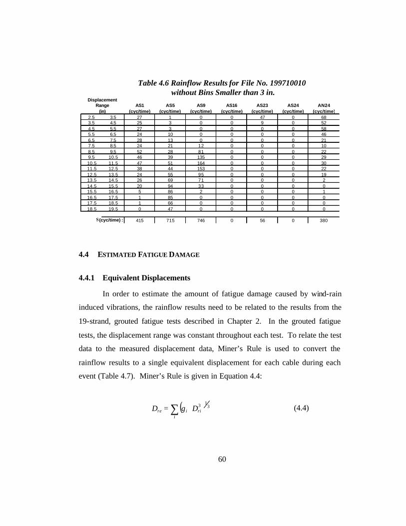
60
Table 4.6 Rainflow Results for File No. 199710010 without Bins Smaller than 3 in.
AS1 AS5 AS9 AS16 AS23 AS24 AN24(cyc/time) (cyc/time) (cyc/time) (cyc/time) (cyc/time) (cyc/time) (cyc/time)
2.5 3.5 27 1 0 0 47 0 683.5 4.5 25 3 0 0 9 0 524.5 5.5 27 3 0 0 0 0 585.5 6.5 24 10 0 0 0 0 466.5 7.5 28 13 0 0 0 0 217.5 8.5 24 21 12 0 0 0 108.5 9.5 52 28 81 0 0 0 229.5 10.5 46 39 135 0 0 0 2910.5 11.5 47 51 164 0 0 0 3011.5 12.5 38 44 153 0 0 0 2212.5 13.5 24 55 95 0 0 0 1913.5 14.5 26 69 71 0 0 0 214.5 15.5 20 94 33 0 0 0 015.5 16.5 5 86 2 0 0 0 116.5 17.5 1 85 0 0 0 0 017.5 18.5 1 66 0 0 0 0 018.5 19.5 0 47 0 0 0 0 0
Σ(cyc/time) : 415 715 746 0 56 0 380
Range(in)
Displacement
4.4 ESTIMATED FATIGUE DAMAGE
4.4.1 Equivalent Displacements
In order to estimate the amount of fatigue damage caused by wind-rain
induced vibrations, the rainflow results need to be related to the results from the
19-strand, grouted fatigue tests described in Chapter 2. In the grouted fatigue
tests, the displacement range was constant throughout each test. To relate the test
data to the measured displacement data, Miner’s Rule is used to convert the
rainflow results to a single equivalent displacement for each cable during each
event (Table 4.7). Miner’s Rule is given in Equation 4.4:
( )∑ ⋅=i
riire DD 313γ (4.4)

61
,where Dre is the equivalent displacement and Dri is the midpoint of each
displacement bin. γi is the proportion of the number of cycles in bin i to the total
number of cycles in all the bins and is calculated using Equation 4.5:
∑
=
ii
ii timecycles
timecycles)/(
)/(γ (4.5)
Table 4.7 Equivalent Displacements for each Cable During each Wind-Rain Vibration Event
File AS1 AS5 AS9 AS16 AS23 AS24 AN24
1997100111 8.5 13.5 13.6 -- 4.3 -- 8.51997100628 10.7 10.5 12.5 -- 4.0 -- 8.21997100710 10.6 14.8 11.7 -- 4.0 -- 8.71997100713 -- -- -- 4.1 4.9 6.9 --199711288 -- -- -- 9.0 10.2 16.0 4.1
1997120718 -- -- -- 6.8 8.7 6.1 13.41997120746 -- -- -- 11.9 -- 4.3 --1998062816 -- -- -- 9.6 11.0 11.5 4.61998062818 -- -- -- 15.1 14.7 17.7 4.0199807038 17.9 19.7 19.4 -- 5.0 6.6 12.3
Once the equivalent displacement amplitude for each cable during each
event was obtained, Miner’s Rule was used again to obtain the overall equivalent
displacement for each cable from all the events combined. To do this the
equivalent displacement for each event was used for Dri and the number of cycles
for each event was used for (cycles/time)i in Equations 4.4 and 4.5 respectively.
The over all equivalent displacement for each cable is provided in Table 4.8.
In addition to the equivalent displacement, the number of cycles that each
cable experiences during a wind-rain event is needed to define the fatigue
damage. To estimate the number of cycles associated with each equivalent
displacement, the average cycles/minute for each cable during each wind-rain

62
vibration event was calculated. The average number of cycles/minute for each
cable is also provided in Table 4.8.
Table 4.8 Overall Equivalent Displacements and Average Cycles per Minute for each Cable
AS1 AS5 AS9 AS16 AS23 AS24 AN24Dre: 9.4 12.1 11.5 11.1 11.6 13.4 7.9
Cycles/min: 33 64 58 70 53 55 41
4.4.2 Estimated Fatigue
To estimate the fatigue damage to the cables due to wind-rain induced
vibration, the overall equivalent displacement for each cable is assumed to be
applied to the cable at the associated cycles per minute during each wind-rain
vibration event. The number of events and length of each event that each of the
cables has undergone is estimated using the JHU database. The length of each
event is conservatively estimated at one minute. One minute is the estimate since
it is the length of each of the records used to create the statistics in the JHU
database and hence it is the maximum possible length of each of the events. The
database has 163,230 records from October 30, 1997 to December 13, 2002. The
number of events is extrapolated to include all the time since the bridge was
constructed in September of 1995.
However, the DAQ system used to record each record was not
operational during the entire period. For that reason, the estimate for the number
of cycles may actually be low and should be increased a reasonable amount to
ensure a conservative estimate. Based on the number of times that the
instrumentation on each cable was discovered to be inoperative, a The total
number of cycles estimated for each cable is increased by certain percentage

63
based on the number of times the instrumentation on each cable was inoperable
between October 30, 1997 and December 13, 2002. Table 4.9 shows the number
of events from the database and the resulting number of cycles for each of the
cables analyzed.
Table 4.9 Total Number of Wind-Rain Cycles for Each Cable
AS1 AS5 AS9 AS16 AS23 AS24 AN24No. of Events: 779 4,182 1,551 1,103 1,103 410 410
Cycles/Min.: 33 64 58 70 53 55 41Total Cycles: 26,027 269,316 90,689 77,534 58,895 22,548 16,702Increase by: 29% 12% 18% 12% 6% 6% 6%
Adjusted Total Cycles: 33,575 301,634 107,013 86,838 62,429 23,901 17,704
4.5 COMPARISON WITH TESTS
So far in the 19-strand grouted tests, less than 2% of the wires had failed at
the anchorage after 500,000 cycles (Poser 2002). Table 4.10 provides a summary
of the number of cycles until the first wire break for the first five 19-strand
specimen. For comparison, Table 4.11 provides a summary of the estimated
fatigue of the Fred Hartman stay-cables. In both tables the “Location of
Displacement” is the distance from the end of the cable to the imposed
displacement or the accelerometer location.
Table 4.10 Summary of the Number of Cycles to the First Wire Break in Test Specimen 1 through 6
Number Displacement Location of First Wire
Specimen Number of Strands (+/- in.) Displacement (ft) BreakCable Stay 1 (grouted)*: 19 1.6 16.5 300,000Cable Stay 2 (grouted)*: 19 1.6 16.5 420,000Cable Stay 3 (grouted): 19 1.6 16.5 1,100,000Cable Stay 4 (grouted): 19 1.1 16.5 2,850,000
Cable Stay 5 (ungrouted): 19 1.6 16.5 **
* (Poser 2002)** No wire breaks occurred in specimen 5 after 5,210,000 Cycles

64
Table 4.11 Summary of Estimated Fatigue for Seven Fred Hartman Stay Cables
Cable Number Equivalent Location of Total Number
ID of Strands Displacement (in.) Displacement (ft) of CyclesAS1: 61 9.4 51 31,233AS5: 43 12.1 52 323,179AS9: 31 11.5 37 108,827
AS16: 31 11.1 38 93,041AS23: 55 11.6 65 70,674AS24: 55 13.4 60 27,057AN24: 55 7.9 63 20,042
Note that all the test specimens experienced a relatively high number of
cycles compared to the bridge cables but the amount of displacement and the
location of the displacements are not the same for both the specimens and the
bridge cables. It is important to note that all of the cables in Table 4.10 are larger
in diameter and have more strands than the 19-strand test specimen. Because of
this difference, the stress induced by the same displacement will be higher in the
bridge cables for the same displacement. Because the FEM models developed on
this project are not able to correlate the displacement of a cable to the stress at the
ends, there is no way to compare these results. Future FEM models should be
able to estimate the stresses in any size cable based on a given displacement and
displacement location. It is anticipated that future researchers will be able to
evaluate the fatigue damage based on a refined FEM model and the results
presented in this chapter.
4.6 RECOMMENDATION FOR FUTURE RESEARCH
Further research needs to be performed to verify the results of this chapter.
The equivalent displacement and cycles/minute are based on a limited number of
records and should include more records of wind-rain induced vibration. To do
this the process should be automated to improve efficiency. In addition the
65
analysis should include all of the cables that were instrumented with
accelerometers so the results can be more easily applied to all the cables on the
bridge.
Another improvement for the analysis would be to analyze each one-
minute segment included in the JHU database. While this may be an arduous
task, it would lead to a much more accurate estimate of the amount of time each
cable has undergone wind-rain induced vibrations. The more accurate estimate
should be less than the estimate presented in this chapter and should also provide
a better confidence level.
When a refined FEM model is complete, these results should be analyzed.
When the stress in the Fred Hartman cables is better understood, the 19-strand
tests can be modified to better resemble the stresses in the bridge cables. In
addition, the results presented in this chapter can be used to estimate the fatigue
damage of each bridge cable due to wind-rain induced vibrations.

66
CHAPTER 5
Summary and Conclusions
This thesis was prepared to assist the research team with the fatigue
analysis of the Fred Hartman Bridge stay cables. While this thesis does not report
the results of any full-scale cable tests, it does provide information to assist the
research team with future research. The three topics discussed in this thesis
include:
1. Static tests of single-strand specimens under tension and bending
and the development of the associated closed-form solutions for a
simply-supported beam and a fixed-fixed beam. The results of the
single-strand test are compared with the 19-strand specimens and
the closed-form solutions.
2. Tensile fatigue testing of representative strand used to construct
the full-scale specimens 1 through 6. The results are compared
with published strand fatigue data and PTI specifications.
3. Characterization of the cable stay vibration data from the Fred
Hartman Bridge. The vibration data were used to estimate the
fatigue damage to the Fred Hartman cables due to wind-rain
induced vibration.
5.1 SINGLE-STRAND BENDING TESTS
The single-strand bending tests provided information about the bending
characteristics of single-strand specimens under tension. The results of these tests

67
and the associated closed-form solutions should assist the research team with
improving the FEM models for the 19-strand specimen. Important information
obtained with these tests includes:
o The strain due to bending is essentially zero 12 in. from the face of
the chuck, which agrees with the closed-form solution, for a fixed-
fixed beam.
o Based on the stiffness comparison between the single-strand tests
and grouted and ungrouted 19-strand tests, it appears that the grout
has only a minor influence on the stiffness of the 19-strand
specimens.
o The single-strand specimens were approximately 2% less stiff than
the stiffness calculated using the closed form solution for a fixed-
fixed beam and approximately 4% more stiff than the stiffness
calculated using the closed-form solution for a simply-supported
beam. This concludes that the two models are upper and lower
bounds to the actual stiffness of the strand.
o The measured response of individual single-strand indicated that
the single-strand specimen became slightly stiffer as mid-point
deflection increased. The most probable reason for the increase in
stiffness is an increase in tension during bending. This
phenomenon was not considered in the closed-form solution.
o An effective EI of 0.94EI can be used in the fixed-fixed beam
solution to attain the observed response of a single strand.
o Based on the moment comparison between the single-strand tests
and the closed-form solutions, it appears that the calculated

68
moment in the strand is less than the closed form solution for the
fixed-fixed beam.
5.2 STRAND TENSION FATIGUE TESTS
The strand tension fatigue tests were used to develop the fatigue
characteristics of the strand used to construct Stay Cable Tests 1 through 6.
Results of the tests indicate that the fatigue characteristic of the strand do not meet
the 1986 or the 2001 PTI specifications. The strand however does fall between
the minimum and mean of strand fatigue data published by Paulson (1983).
Recommendations for the strand tension fatigue tests include:
o Additional strand fatigue tests should be performed at stress ranges
other than 20, 30, and 40 ksi. to develop a complete S-N curve for
the strand
o When the stress in the strands of the 19-strand specimens is better
defined, strand fatigue tests should be performed at those stress
ranges. With the additional information from these tests, the
failure mechanism of the wires in the 19-strand specimens and
hence the Fred Hartman bridge should be better understood.
o A test should be developed to conduct fatigue tests of grouted
single strands. These results will assist in the identification of
fretting and the associated reduction in fatigue life due to fretting.
5.3 FRED HARTMAN CABLE VIBRATION CHARACTERIZATION
Acceleration records from cable vibration events on the Fred Hartman
Bridge were characterized in terms of the following characteristics:

69
o The displacement of cable at the accelerometer location
o Primary vibration frequencies and mode of the cable vibration
o The equivalent displacement and the associated cycles/minute for
each cable
o The total number of cycles that each cable has undergone since
construction of the bridge in September of 1995.
After characterization of the cable stay vibrations the calculated
displacement record was used to estimate the equivalent displacement of each
bridge cable analyzed. Using the database developed by researchers at Johns
Hopkins the total number of cycles that each cable experienced was also
estimated. It is not possible to relate these results to fatigue damage because of
the differences in calculated displacement location and cable size. However, it
was concluded that a refined FEM model needs to be developed to relate the
deflection of the cables to stress at the ends. With this refined model, the results
presented in Chapter 4 can be used to evaluate the fatigue damage in the Fred
Hartman stay-cables.
The following are recommendations for improving this analysis:
o More than ten wind-rain vibrations records should be
characterized. If possible, the process should be automated for
efficiency. In addition, all the cables that had accelerometers
should be included in the analysis.
o The one-minute acceleration records from the database should be
analyzed for a better prediction of the total number of cycles that
each cable has undergone. This process should also be automated
to improve efficiency.

70
o After the refined FEM model is complete, the stresses in the Fred
Hartman cables should be estimated so that the 19-strand tests can
be adjusted to simulate the bending stresses seen in the bridge
cables. The results of these improved tests should provide better
estimates of the actual fatigue damage.

108
Appendix A
Closed-Form Solutions
The derivation of both closed-form solutions were developed with the
following parameters:
o The strand is viewed as a tension strut with a transverse force at mid-
span
o To include secondary bending effects due to the tension in the strand,
the free-body diagram (FBD) includes an initial deflection due to the
transverse load. This is similar to the derivation of a compression
member with secondary bending (i.e. Euler buckling), except the
solution is stable due to the tension in the strand.
o Deformation due to shear was ignored due to the large span-to-depth
ratio of the strand.
o Because the transverse load is located at mid-span, the solutions for
both cases are symmetric. Therefore the solutions are derived for only
half of the beam.
A.1 FIXED-FIXED BEAM WITH AXIAL TENSION AND BENDING
Figure A.1 shows the free body diagram used to establish the equilibrium
equation for the fixed-fixed beam. The equilibrium equation is developed by
summing the moments about an arbitrary point at a distance x, along the beam.

109
Figure A.1 Fixed-Fixed Beam Free Body Diagram
A.1.1 Derivation
Equilibrium Equation Substitutions
M x( ) R x⋅ T ν x( )⋅− Mo−
E− I⋅ 2x
ν x( )d
d
2⋅ R x⋅ T ν x( )⋅− Mo− M x( ) E− I 2
xν x( )d
d
2⋅
2x
ν x( )d
d
2 T
E I⋅ν x( )⋅−
P−
2 E⋅ I⋅x⋅
Mo
E I⋅+ R
P
2
Governing Differential Equation
2x
ν x( )d
d
2λ
2ν x( )⋅−
P−
2 E⋅ I⋅x⋅
Mo
E I⋅+ λ
2 T
E I⋅
General Solutions
ν x( ) A sinh λ x⋅( )⋅ B cosh λ x⋅( )⋅+ C x⋅+ D+
xν x( )d
dA λ⋅ cosh λ x⋅( )⋅ B λ⋅ sinh λ x⋅( )⋅+ C+
2x
ν x( )d
d
2A λ
2⋅ sinh λ x⋅( )⋅ B λ
2⋅ cosh λ x⋅( )⋅+
T
TR
Mo M(x)
x
υ (x)

110
Solve for C and D
2x
ν x( )d
d
2λ
2ν x( )⋅− C x⋅ D+( )− λ
2⋅
C− λ2
⋅ D λ2
⋅−P−
2 E⋅ I⋅x⋅
Mo
E I⋅+
C− λ2
⋅P−
2 E⋅ I⋅x⋅ D− λ
2⋅
Mo
E I⋅
CP
2TD
Mo−
T
Use Boundry Conditions to Solve for A and B
ν 0( ) 0
BMo
T
xν 0( )d
d0
AP−
2T λ⋅
Particular Solutions for Fixed-Fixed Beam
ν x( )P−
2T λ⋅sinh λ x⋅( )⋅
Mo
Tcosh λ x⋅( )⋅+
P
2Tx⋅+
Mo
T−
xν x( )d
d
P−
2 T⋅cosh λ x⋅( )⋅
Mo
Tλ⋅ sinh λ x⋅( )⋅+
P
2 T⋅+
2x
ν x( )d
d
2 P−
2 T⋅λ⋅ sinh λ x⋅( )⋅
Mo
Tλ
2⋅ cosh λ x⋅( )⋅+

111
Solve for Mo
since load is at mid-span,
Mo ML
2
and,
xν
L
2
dd
0
MoP L⋅
2
coshL
2λ⋅
1−
sinhL
2λ⋅
⋅
A.1.2 Fixed-Fixed Beam Deflected Shape
0.0
0.2
0.4
0.6
0.8
1.0
1.2
1.4
1.6
1.8
2.0
0 1/8 1/4 3/8 1/2
Location, (x/L)
Def
lect
ion
(in
.)
Figure A.2 Fixed-Fixed Beam Deflection Diagram
T = 23.6 kip
P = 514 lb
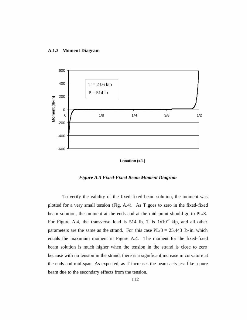
112
A.1.3 Moment Diagram
-600
-400
-200
0
200
400
600
0 1/8 1/4 3/8 1/2
Location (x/L)
Mom
ent (
lb-in
)
Figure A.3 Fixed-Fixed Beam Moment Diagram
To verify the validity of the fixed-fixed beam solution, the moment was
plotted for a very small tension (Fig. A.4). As T goes to zero in the fixed-fixed
beam solution, the moment at the ends and at the mid-point should go to PL/8.
For Figure A.4, the transverse load is 514 lb, T is 1x10⁻⁷ kip, and all other
parameters are the same as the strand. For this case PL/8 = 25,443 lb- in. which
equals the maximum moment in Figure A.4. The moment for the fixed-fixed
beam solution is much higher when the tension in the strand is close to zero
because with no tension in the strand, there is a significant increase in curvature at
the ends and mid-span. As expected, as T increases the beam acts less like a pure
beam due to the secondary effects from the tension.
T = 23.6 kip
P = 514 lb

113
-30,000
-20,000
-10,000
0
10,000
20,000
30,000
0 1/8 1/4 3/8 1/2
Location (x/L)
Mom
ent
(lb-in
)
Figure A.4 Fixed-Fixed Beam Moment Diagram for T ˜ 0 kip
T = 0 kip
P = 514 lb

114
A.2 SIMPLY SUPPORTED BEAM WITH AXIAL TENSION AND BENDING
Figure A.4 shows the free body diagram used to develop the equilibrium
equation for the simply-supported solution. The primary difference between the
fixed-fixed solution and the simply-supported solution is the reaction moment at
the beam ends. The deflection diagram (Fig. A.4) and the moment diagram (Fig.
A.6) are associated with a transverse load of 482 lb which results in a stiffness of
241 lb/in.
Figure A.5 Simply-Supported Beam Free Body Diagram
T
TR
M(x)
x
υ (x)

115
A.2.1 Derivation
Equilibrium Equation Substitutions
M x( ) R x⋅ T ν x( )⋅−
M x( ) E− I 2x
ν x( )d
d
2⋅
E− I⋅ 2x
ν x( )d
d
2⋅ R x⋅ T ν x( )⋅−
2x
ν x( )d
d
2 T
E I⋅ν x( )⋅−
P−
2 E⋅ I⋅x⋅ R
P
2
Governing Differential Equation
λ2 T
E I⋅2x
ν x( )d
d
2λ
2ν x( )⋅−
P−
2 E⋅ I⋅x⋅
General Solutions
ν x( ) A sinh λ x⋅( )⋅ B cosh λ x⋅( )⋅+ C x⋅+
xν x( )d
dA λ⋅ cosh λ x⋅( )⋅ B λ⋅ sinh λ x⋅( )⋅+ C+
2x
ν x( )d
d
2A λ
2⋅ sinh λ x⋅( )⋅ B λ
2⋅ cosh λ x⋅( )⋅+

116
Solve for C
2xν x( )d
d
2λ
2ν x( )⋅− C− x⋅ λ
2⋅
C− λ2
⋅P−
2 E⋅ I⋅x⋅
C− λ2
⋅P−
2 E⋅ I⋅x⋅
CP2T
Use Boundry Conditions to Solve for A and B
ν 0( ) 0
B 0
xν
L
2
dd
0
AP−
2T λ⋅ cosh λL2
⋅
⋅
Particular Solutions for Simply-Supported Beam
ν x( )P−
2 T⋅ λ⋅
sinh λ x⋅( )
cosh λL2
⋅
⋅P
2 T⋅x⋅+
xν x( )d
d
P−2 T⋅
cosh λ x⋅( )
cosh λL2
⋅
⋅P
2 T⋅+
2x
ν x( )d
d
2 P−2 T⋅
λ⋅sinh λ x⋅( )
cosh λL2
⋅
⋅

117
A.2.2 Simply-Supported Beam Defected Shape
Figure A.6 shows the deflected shape for a simply-supported beam with a
tension of 23.6 kip and a transverse load at the midpoint of 482 lb. This correlates
to a maximum deflection of 2.0 in.
0.0
0.2
0.4
0.6
0.8
1.0
1.2
1.4
1.6
1.8
2.0
0 1/8 1/4 3/8 1/2
Location (x/L)
Def
lect
ion
(in)
Figure A.6 Simply-Supported Deflected Shape
T = 23.6 kip
P = 482 lb

118
A.2.3 Moment Diagram
0
100
200
300
400
500
600
0 1/8 1/4 3/8 1/2
Location (x/L)
Mom
ent (
lb-in
.)
Figure A.7 Simply-Supported Beam Moment Diagram
T = 23.6 kip
P = 482 lb

119
To verify the validity of the simply-supported beam solution, the moment
was plotted for a very small tension (Fig. A.8). As T goes to zero in the simply-
supported beam solution, the moment at the mid-point should go to PL/4. For
Figure A.4, the transverse load is 482 lb, T is 1x10⁻⁷ kip, and all other parameters
are the same as the strand. For this case PL/4 = 47,713 lb- in. which equals the
maximum moment in Figure A.8. Similar to the fixed-fixed solution, when T is
close to zero the moment in the strand is significantly increased due to the
increase in curvature at mid-span. As expected, as T increases the beam acts less
like a pure beam due to the secondary effects from the tension.
0
10,000
20,000
30,000
40,000
50,000
60,000
0 1/8 1/4 3/8 1/2
Location (x/L)
Mom
ent (
lb-in
.)
Figure A.8 Simply-supported Beam Moment Diagram for T ˜ 0 kip
T = 23.6 kip
P = 482 lb

120
Appendix B
Single-Strand Bending Tests
The single-strand bending tests were performed with three different strand
specimens. For each specimen two or three tests were performed at different
prestress levels. Note that each test was repeated at least twice. Only one cycle
of each test is included in this appendix because the responses of the tests were
within 5 % of each other for each cycle. Also note that tests performed at low
prestress levels (less than 4 kip) are not included in this appendix because the
variation in strain was extremely small.
Strains measured by all functioning gages are plotted against mid-span
deflection of the strand in this appendix. Note that at least one of the strain gages
failed to yield useful data due to damage or de-bonding from the strand in all the
tests. Data from these gages are not plotted. The strand specimen number and the
test number are indicated in the title of each plot and the gage location is indicated
within each plot. Table B.1 provides a summary of the tests and indicates which
strain gage data was plotted for each test.
Also included in this appendix is a copy of the manufacturer’s
specification sheet for the strand used in the single-strand bending tests, the strand
tension fatigue tests, and the full-sized stay-cable bending fatigue tests
(Fig. B.17).
In addition, this appendix includes data collected for verification of the
size of the strand. For a strand sample, the area of each wire was measured and
tabula ted (Fig. B.18).

121
Table B.1 Single Strand Test Summary
Prestress
Strand Test (kip) A1 A2 A3 A4 A5 A6 B1 B2 B3 B4 B5 B61 1 7.5 X X X X X X X1 2 21.4 X X X X X X X2 1 14.5 X X X X X X X X2 2 20.9 X X X X X X X X2 3 23.3 X X X X X X X X3 1 21.9 X X X X X X X X X X3 2 23.5 X X X X X X X X X X3 3 30.9 X X X X X X X X X X
X indicates a strain gage that worked throughout the test. These strain gages are plotted.
Strain Gages

122
-80
-60
-40
-20
0
20
40
60
80
100
120
0.0 0.5 1.0 1.5 2.0
Deflection (in.)
Str
ain
(10-6
) A1A3A5A6
Figure B.1 Strand 1, Test 1 at a Prestress of 7.5 kip
-40
-20
0
20
40
60
80
0.0 0.5 1.0 1.5 2.0
Deflection (in.)
Str
ain
(10
-6)
B1
B2B3
Figure B.2 Strand 1, Test 1 at a Prestress of 7.5 kip
Location B 2.5 in. from chuck.
Location A 1.6 in. from chuck.

123
-250
-200
-150
-100
-50
0
50
100
150
200
250
300
0.0 0.5 1.0 1.5 2.0
Deflection (in.)
Str
ain
(10
-6) A1
A3A5A6
Figure B.3 Strand 1, Test 2 at a Prestress of 21.4 kip
-100
-50
0
50
100
150
200
250
0.0 0.5 1.0 1.5 2.0
Deflection (in.)
Str
ain
(10-6
)
B1
B2B3
Figure B.4 Strand 1, Test 2 at a Prestress of 21.4 kip
Location A 1.6 in. from chuck.
Location B 2.5 in. from chuck.

124
-60
-40
-20
0
20
40
60
80
100
120
140
0.0 0.2 0.4 0.6 0.8 1.0 1.2 1.4 1.6 1.8 2.0 2.2
Deflection (in)
Str
ain
(10
-6) A1
A2
A3
A5
A6
Figure B.5 Strand 2, Test 1 at a Prestress of 14.5 kip
-20
-10
0
10
20
30
40
50
60
0.0 0.2 0.4 0.6 0.8 1.0 1.2 1.4 1.6 1.8 2.0 2.2
Deflection (in)
Str
ain
(10-6
)
B1
B2
B3
Figure B.6 Strand 2, Test 1 at a Prestress of 14.5 kip
Location A 2.1 in. from chuck.
Location B 3.1 in. from chuck.

125
-200
-100
0
100
200
300
400
500
0.0 0.5 1.0 1.5 2.0 2.5
Deflection (in.)
Str
ain
(10-6
) A1A2A3A5A5
Figure B.7 Strand 2, Test 2 at a Prestress of 20.9 kip
-50
0
50
100
150
200
250
0.0 0.5 1.0 1.5 2.0 2.5
Deflection (in.)
Str
ain
(10-6
)
B1B2B3
Figure B.8 Strand 2, Test 2 at a Prestress of 20.9 kip
Location A 2.1 in. from chuck.
Location B 3.1 in. from chuck.

126
-200
-100
0
100
200
300
400
500
600
0.0 0.5 1.0 1.5 2.0 2.5
Deflection (in.)
Str
ain
(10
-6) A1
A2A3A5A6
Figure B.9 Strand 2, Test 3at a Prestress of 23.3 kip
-50
0
50
100
150
200
250
300
350
0.0 0.5 1.0 1.5 2.0 2.5
Deflection (in.)
Str
ain
(10
-6)
B1
B2B3
Figure B.10 Strand 2, Test 3 at a Prestress of 23.3 kip
Location A 2.1 in. from chuck.
Location B 3.1 in. from chuck.

127
-300
-200
-100
0
100
200
300
400
500
0 0.5 1 1.5 2 2.5
Deflection (in.)
Str
ain
(10
-6) A1
A2
A3
A5
A6
Figure B.11 Strand 3, Test 1 at a Prestress of 21.9 kip
-20
0
20
40
60
80
100
120
0 0.5 1 1.5 2 2.5
Deflection (in.)
Str
ain
(10-6
) B1
B2
B3
B4
B5
Figure B.12 Strand 3, Test 1 at a Prestress of 21.9 kip
Location A 1.8 in. from chuck.
Location B 2.5 in. from chuck.

128
-400
-300
-200
-100
0
100
200
300
400
0.00 0.50 1.00 1.50 2.00 2.50
Deflection (in.)
Str
ain
(10
-6) A1
A2A3
A5A6
Figure B.13 Strand 3, Test 2 at a Prestress of 23.5 kip
0
10
20
30
40
50
60
70
80
90
100
0.00 0.50 1.00 1.50 2.00 2.50
Deflection (in.)
Str
ain
(10-6
) B1B2B3B4
B5
Figure B.14 Strand 3, Test 2 at a Prestress of 23.5 kip
Location A 1.8 in. from chuck.
Location B 2.5 in. from chuck.

129
-300
-200
-100
0
100
200
300
400
500
0 0.5 1 1.5 2 2.5
Deflection (in.)
Str
ain
(10
-6) A1
A2A3A5A6
Figure B.15 Strand 3, Test 3 at a Prestress of 30.8 kip
-20
0
20
40
60
80
100
120
140
0 0.5 1 1.5 2 2.5
Deflection (in.)
Str
ain
(10
-6) B1
B2
B3B4
B5
Figure B.16 Strand 3, Test 3 at a Prestress of 30.8 kip
Location A 1.8 in. from chuck.
Location B 2.5 in. from chuck.

130
Figure B.17 Strand Specification Sheet

131
A sample strand was used to measure the area of each wire to verify the
size of the strand used in the single strand tests and the full-scale specimens 1
through 6. The measure the area of each wire, the sample strand was unwound
into 7 separate wires. Each wire was measured to be 6 1/16-in. long. Each wire
was placed in a graduated cylinder filled with water. The displacement of each
wire was recorded and the area of each wire was ten calculated (Fig. B.18). The
total measured area of the strand was essentially the same as the area provided by
the manufacturer (Fig. B.17).
Wire No. Wire Location Length (in) Volume (mL) Volume (in3) Area (in2)1 outer 6.1875 3.13 0.191 0.0312 outer 6.1875 3.12 0.190 0.0313 outer 6.1875 3.13 0.191 0.0314 outer 6.1875 3.12 0.190 0.0315 outer 6.1875 3.14 0.192 0.0316 outer 6.1875 3.13 0.191 0.0317 inner 6.1875 3.30 0.201 0.033
Total Area (in2): 0.218 Figure B.18 Strand Size Verification

132
Appendix C
Rainflow Analysis Results
The rainflow analysis results from CRUNCH (Buhl 2002) are presented in
this appendix. For each wind-rain vibration file there are two rainflow results
tables provided. The first is the raw output from CRUNCH and the second is the
modified rainflow counts excluding all cycles with a displacement range of less
than 3 in. For a thorough explanation of the CRUNCH rainflow algorithm see
Buhl (2002).
In each table, the amplitude range of each bin is 1 in. except the first bin
which has an amplitude range of ½ in. The cycle counts for each cable are
provided in units of cycles per time. Because each displacement record is 5
minutes, the number of cycles occurring in 5 minutes is tabulated. The file
numbers associated with each table correlate to the date the file was recorded.
The first 8 numbers represent the year, month, and day respectively that the file
was recorded. The last one or two digits corresponds to the number of the
recording on that date. For example file number 1997100111 is the 11th file
recorded on October 1, 1997. The “D_” prefix on each file name indicates that
the file was a displacement history.
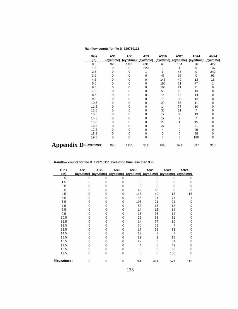
133
Appendix D
Rainflow counts for file D_199710111
Bins AS1 AS5 AS9 AS16 AS23 AS24 AN24(in) (cyc/time) (cyc/time) (cyc/time) (cyc/time) (cyc/time) (cyc/time) (cyc/time)0.5 926 1151 691 60 184 26 4221.5 0 0 220 0 1 0 1372.5 0 0 1 1 45 0 2423.5 0 0 0 42 58 0 934.5 0 0 0 148 40 13 185.5 0 0 0 196 21 77 16.5 0 0 0 108 21 21 07.5 0 0 0 53 15 13 08.5 0 0 0 14 13 14 09.5 0 0 0 16 36 12 0
10.5 0 0 0 29 83 11 011.5 0 0 0 14 77 10 012.5 0 0 0 30 51 7 013.5 0 0 0 17 38 13 014.5 0 0 0 17 7 7 015.5 0 0 0 29 1 15 016.5 0 0 0 27 0 31 017.5 0 0 0 4 0 49 018.5 0 0 0 0 0 98 019.5 0 0 0 0 0 180 0
Σ(cyc/time) : 926 1151 912 805 691 597 913
Rainflow counts for file D_199710111 excluding bins less than 3 in.
Bins AS1 AS5 AS9 AS16 AS23 AS24 AN24(in) (cyc/time) (cyc/time) (cyc/time) (cyc/time) (cyc/time) (cyc/time) (cyc/time)0.5 0 0 0 0 0 0 01.5 0 0 0 0 0 0 02.5 0 0 0 0 0 0 03.5 0 0 0 42 58 0 934.5 0 0 0 148 40 13 185.5 0 0 0 196 21 77 16.5 0 0 0 108 21 21 07.5 0 0 0 53 15 13 08.5 0 0 0 14 13 14 09.5 0 0 0 16 36 12 010.5 0 0 0 29 83 11 011.5 0 0 0 14 77 10 012.5 0 0 0 30 51 7 013.5 0 0 0 17 38 13 014.5 0 0 0 17 7 7 015.5 0 0 0 29 1 15 016.5 0 0 0 27 0 31 017.5 0 0 0 4 0 49 018.5 0 0 0 0 0 98 019.5 0 0 0 0 0 180 0
Σ(cyc/time) : 0 0 0 744 461 571 112

134
Rainflow counts for file D_199807038
Bins AS1 AS5 AS9 AS16 AS23 AS24 AN24(in) (cyc/time) (cyc/time) (cyc/time) (cyc/time) (cyc/time) (cyc/time) (cyc/time)0.5 986 605 38 0 69 474 4931.5 0 0 0 0 89 30 302.5 0 0 0 0 46 36 83.5 0 0 0 1 21 31 34.5 0 0 0 0 22 16 15.5 0 0 0 170 35 38 36.5 0 0 0 231 41 78 17.5 0 0 0 187 45 52 08.5 0 0 0 91 72 6 19.5 0 0 0 61 97 0 2
10.5 0 0 0 2 87 0 211.5 0 0 0 0 44 0 112.5 0 0 0 0 9 0 113.5 0 0 0 0 0 0 014.5 0 0 0 0 0 0 015.5 0 0 0 0 0 0 116.5 0 0 0 0 0 0 017.5 0 0 0 0 0 0 118.5 0 0 0 0 0 0 019.5 0 0 0 0 0 0 4
Σ(cyc/time) : 986 605 38 743 677 761 552
Rainflow counts for file D_199807038 excluding bins less than 3 in.
Bins AS1 AS5 AS9 AS16 AS23 AS24 AN24(in) (cyc/time) (cyc/time) (cyc/time) (cyc/time) (cyc/time) (cyc/time) (cyc/time)0.5 0 0 0 0 0 0 01.5 0 0 0 0 0 0 02.5 0 0 0 0 0 0 03.5 0 0 0 1 21 31 34.5 0 0 0 0 22 16 15.5 0 0 0 170 35 38 36.5 0 0 0 231 41 78 17.5 0 0 0 187 45 52 08.5 0 0 0 91 72 6 19.5 0 0 0 61 97 0 210.5 0 0 0 2 87 0 211.5 0 0 0 0 44 0 112.5 0 0 0 0 9 0 113.5 0 0 0 0 0 0 014.5 0 0 0 0 0 0 015.5 0 0 0 0 0 0 116.5 0 0 0 0 0 0 017.5 0 0 0 0 0 0 118.5 0 0 0 0 0 0 019.5 0 0 0 0 0 0 4
Σ(cyc/time) : 0 0 0 743 473 221 21

135
Rainflow counts for file D_199711288
Bins AS1 AS5 AS9 AS16 AS23 AS24 AN24(in) (cyc/time) (cyc/time) (cyc/time) (cyc/time) (cyc/time) (cyc/time) (cyc/time)0.5 1042 1068 1227 48 888 941 8731.5 0 55 3 78 28 58 02.5 0 0 0 94 0 43 03.5 0 0 0 49 0 23 04.5 0 0 0 19 0 14 05.5 0 0 0 19 0 4 06.5 0 0 0 34 0 0 07.5 0 0 0 79 0 0 08.5 0 0 0 47 0 0 09.5 0 0 0 55 0 0 0
10.5 0 0 0 40 0 0 011.5 0 0 0 22 0 0 012.5 0 0 0 9 0 0 013.5 0 0 0 8 0 0 014.5 0 0 0 48 0 0 015.5 0 0 0 63 0 0 016.5 0 0 0 49 0 0 017.5 0 0 0 21 0 0 018.5 0 0 0 2 0 0 019.5
Σ(cyc/time) : 1042 1123 1230 784 916 1083 873
Rainflow counts for file D_199711288 excluding bins less than 3 in.
Bins AS1 AS5 AS9 AS16 AS23 AS24 AN24(in) (cyc/time) (cyc/time) (cyc/time) (cyc/time) (cyc/time) (cyc/time) (cyc/time)0.5 0 0 0 0 0 0 01.5 0 0 0 0 0 0 02.5 0 0 0 0 0 0 03.5 0 0 0 49 0 23 04.5 0 0 0 19 0 14 05.5 0 0 0 19 0 4 06.5 0 0 0 34 0 0 07.5 0 0 0 79 0 0 08.5 0 0 0 47 0 0 09.5 0 0 0 55 0 0 0
10.5 0 0 0 40 0 0 011.5 0 0 0 22 0 0 012.5 0 0 0 9 0 0 013.5 0 0 0 8 0 0 014.5 0 0 0 48 0 0 015.5 0 0 0 63 0 0 016.5 0 0 0 49 0 0 017.5 0 0 0 21 0 0 018.5 0 0 0 2 0 0 019.5 0 0 0 0 0 0 0
Σ(cyc/time) : 0 0 0 564 0 41 0

136
Rainflow counts for file D_1997100628
Bins AS1 AS5 AS9 AS16 AS23 AS24 AN24(in) (cyc/time) (cyc/time) (cyc/time) (cyc/time) (cyc/time) (cyc/time) (cyc/time)0.5 1390 1128 1249 209 356 10 5571.5 0 0 0 146 58 1 02.5 0 0 0 135 165 17 03.5 0 0 0 175 125 44 04.5 0 0 0 70 45 43 05.5 0 0 0 5 99 72 06.5 0 0 0 0 13 99 07.5 0 0 0 0 0 133 08.5 0 0 0 0 0 121 09.5 0 0 0 0 0 39 0
10.5 0 0 0 0 0 0 011.5 0 0 0 0 0 0 012.5 0 0 0 0 0 0 013.5 0 0 0 0 0 0 014.5 0 0 0 0 0 0 015.5 0 0 0 0 0 0 016.5 0 0 0 0 0 0 017.5 0 0 0 0 0 0 018.5 0 0 0 0 0 0 019.5 0 0 0 0 0 0 0
Σ(cyc/time) : 1390 1128 1249 740 861 579 557
Rainflow counts for file D_1997100628 excluding bins less than 3 in.
Bins AS1 AS5 AS9 AS16 AS23 AS24 AN24(in) (cyc/time) (cyc/time) (cyc/time) (cyc/time) (cyc/time) (cyc/time) (cyc/time)0.5 0 0 0 0 0 0 01.5 0 0 0 0 0 0 02.5 0 0 0 0 0 0 03.5 0 0 0 175 125 44 04.5 0 0 0 70 45 43 05.5 0 0 0 5 99 72 06.5 0 0 0 0 13 99 07.5 0 0 0 0 0 133 08.5 0 0 0 0 0 121 09.5 0 0 0 0 0 39 0
10.5 0 0 0 0 0 0 011.5 0 0 0 0 0 0 012.5 0 0 0 0 0 0 013.5 0 0 0 0 0 0 014.5 0 0 0 0 0 0 015.5 0 0 0 0 0 0 016.5 0 0 0 0 0 0 017.5 0 0 0 0 0 0 018.5 0 0 0 0 0 0 019.5 0 0 0 0 0 0 0
Σ(cyc/time) : 0 0 0 250 282 551 0

137
Rainflow counts for file D_1997100710
Bins AS1 AS5 AS9 AS16 AS23 AS24 AN24(in) (cyc/time) (cyc/time) (cyc/time) (cyc/time) (cyc/time) (cyc/time) (cyc/time)0.5 425 3 1 1310 723 1059 4681.5 45 0 0 41 200 46 612.5 35 0 0 0 118 0 793.5 27 1 0 0 47 0 684.5 25 3 0 0 9 0 525.5 27 3 0 0 0 0 586.5 24 10 0 0 0 0 467.5 28 13 0 0 0 0 218.5 24 21 12 0 0 0 109.5 52 28 81 0 0 0 2210.5 46 39 135 0 0 0 2911.5 47 51 164 0 0 0 3012.5 38 44 153 0 0 0 2213.5 24 55 95 0 0 0 1914.5 26 69 71 0 0 0 215.5 20 94 33 0 0 0 016.5 5 86 2 0 0 0 117.5 1 85 0 0 0 0 018.5 1 66 0 0 0 0 019.5 0 47 0 0 0 0 0
Σ(cyc/time) : 920 718 747 1351 1097 1105 988
Rainflow counts for file D_1997100710 excluding bins less than 3 in.
Bins AS1 AS5 AS9 AS16 AS23 AS24 AN24(in) (cyc/time) (cyc/time) (cyc/time) (cyc/time) (cyc/time) (cyc/time) (cyc/time)0.5 0 0 0 0 0 0 01.5 0 0 0 0 0 0 02.5 0 0 0 0 0 0 03.5 27 1 0 0 47 0 684.5 25 3 0 0 9 0 525.5 27 3 0 0 0 0 586.5 24 10 0 0 0 0 467.5 28 13 0 0 0 0 218.5 24 21 12 0 0 0 109.5 52 28 81 0 0 0 2210.5 46 39 135 0 0 0 2911.5 47 51 164 0 0 0 3012.5 38 44 153 0 0 0 2213.5 24 55 95 0 0 0 1914.5 26 69 71 0 0 0 215.5 20 94 33 0 0 0 016.5 5 86 2 0 0 0 117.5 1 85 0 0 0 0 018.5 1 66 0 0 0 0 019.5 0 47 0 0 0 0 0
Σ(cyc/time) : 415 715 746 0 56 0 380

138
Rainflow counts for file D_1997100713
Bins AS1 AS5 AS9 AS16 AS23 AS24 AN24(in) (cyc/time) (cyc/time) (cyc/time) (cyc/time) (cyc/time) (cyc/time) (cyc/time)0.5 251 22 72 1051 59 561 721.5 59 24 27 167 172 416 472.5 30 25 46 1 248 24 253.5 28 17 60 0 267 0 364.5 20 27 43 0 94 0 335.5 42 53 50 0 3 0 646.5 30 52 15 0 0 0 567.5 37 93 27 0 0 0 1138.5 59 66 42 0 0 0 1469.5 57 91 42 0 0 0 12810.5 38 89 27 0 0 0 8711.5 53 120 59 0 0 0 2612.5 21 106 100 0 0 0 613.5 29 80 61 0 0 0 514.5 23 60 79 0 0 0 015.5 28 22 40 0 0 0 016.5 12 1 33 0 0 0 017.5 9 0 24 0 0 0 018.5 2 0 37 0 0 0 019.5 0 0 4 0 0 0 0
Σ(cyc/time) : 828 948 888 1219 843 1001 844
Rainflow counts for file D_1997100713 excluding bins less than 3 in.
Bins AS1 AS5 AS9 AS16 AS23 AS24 AN24(in) (cyc/time) (cyc/time) (cyc/time) (cyc/time) (cyc/time) (cyc/time) (cyc/time)0.5 0 0 0 0 0 0 01.5 0 0 0 0 0 0 02.5 0 0 0 0 0 0 03.5 28 17 60 0 267 0 364.5 20 27 43 0 94 0 335.5 42 53 50 0 3 0 646.5 30 52 15 0 0 0 567.5 37 93 27 0 0 0 1138.5 59 66 42 0 0 0 1469.5 57 91 42 0 0 0 12810.5 38 89 27 0 0 0 8711.5 53 120 59 0 0 0 2612.5 21 106 100 0 0 0 613.5 29 80 61 0 0 0 514.5 23 60 79 0 0 0 015.5 28 22 40 0 0 0 016.5 12 1 33 0 0 0 017.5 9 0 24 0 0 0 018.5 2 0 37 0 0 0 019.5 0 0 4 0 0 0 0
Σ(cyc/time) : 488 877 743 0 364 0 700

139
Rainflow counts for file D_1997120718
Bins AS1 AS5 AS9 AS16 AS23 AS24 AN24(in) (cyc/time) (cyc/time) (cyc/time) (cyc/time) (cyc/time) (cyc/time) (cyc/time)0.5 87 5 9 1250 527 538 2111.5 0 0 1 203 248 418 272.5 0 4 0 2 144 71 333.5 1 7 0 0 65 6 1034.5 16 18 0 0 42 0 855.5 44 27 0 0 12 0 916.5 90 42 0 0 1 0 537.5 102 72 15 0 0 0 778.5 113 59 29 0 0 0 939.5 74 77 55 0 0 0 5410.5 49 57 70 0 0 0 3011.5 26 55 61 0 0 0 2912.5 29 69 110 0 0 0 2213.5 10 80 87 0 0 0 1014.5 3 63 65 0 0 0 2015.5 0 64 73 0 0 0 716.5 0 81 88 0 0 0 117.5 0 51 54 0 0 0 018.5 0 48 34 0 0 0 019.5 0 72 6 0 0 0 0
Σ(cyc/time) : 644 951 757 1455 1039 1033 946
Rainflow counts for file D_1997120718 excluding bins less than 3 in.
Bins AS1 AS5 AS9 AS16 AS23 AS24 AN24(in) (cyc/time) (cyc/time) (cyc/time) (cyc/time) (cyc/time) (cyc/time) (cyc/time)0.5 0 0 0 0 0 0 01.5 0 0 0 0 0 0 02.5 0 0 0 0 0 0 03.5 1 7 0 0 65 6 1034.5 16 18 0 0 42 0 855.5 44 27 0 0 12 0 916.5 90 42 0 0 1 0 537.5 102 72 15 0 0 0 778.5 113 59 29 0 0 0 939.5 74 77 55 0 0 0 5410.5 49 57 70 0 0 0 3011.5 26 55 61 0 0 0 2912.5 29 69 110 0 0 0 2213.5 10 80 87 0 0 0 1014.5 3 63 65 0 0 0 2015.5 0 64 73 0 0 0 716.5 0 81 88 0 0 0 117.5 0 51 54 0 0 0 018.5 0 48 34 0 0 0 019.5 0 72 6 0 0 0 0
Σ(cyc/time) : 557 942 747 0 120 6 675

140
Rainflow counts for file D_1997120746
Bins AS1 AS5 AS9 AS16 AS23 AS24 AN24(in) (cyc/time) (cyc/time) (cyc/time) (cyc/time) (cyc/time) (cyc/time) (cyc/time)0.5 486 34 40 839 810 110 2551.5 74 5 0 218 292 111 142.5 54 0 0 17 104 119 283.5 67 3 0 0 26 161 184.5 49 8 0 0 2 199 425.5 17 9 0 0 1 137 456.5 8 11 2 0 0 13 397.5 4 9 23 0 0 1 428.5 18 17 61 0 0 0 619.5 36 31 55 0 0 0 6210.5 81 24 78 0 0 0 5111.5 39 32 60 0 0 0 3612.5 10 34 72 0 0 0 3113.5 5 19 73 0 0 0 2414.5 0 25 51 0 0 0 1115.5 0 14 64 0 0 0 216.5 0 12 77 0 0 0 217.5 0 10 83 0 0 0 018.5 0 14 38 0 0 0 019.5 0 442 10 0 0 0 0
Σ(cyc/time) : 948 753 787 1074 1235 851 763
Rainflow counts for file D_1997120746 excluding bins less than 3 in.
Bins AS1 AS5 AS9 AS16 AS23 AS24 AN24(in) (cyc/time) (cyc/time) (cyc/time) (cyc/time) (cyc/time) (cyc/time) (cyc/time)0.5 0 0 0 0 0 0 01.5 0 0 0 0 0 0 02.5 0 0 0 0 0 0 03.5 67 3 0 0 26 161 184.5 49 8 0 0 2 199 425.5 17 9 0 0 1 137 456.5 8 11 2 0 0 13 397.5 4 9 23 0 0 1 428.5 18 17 61 0 0 0 619.5 36 31 55 0 0 0 6210.5 81 24 78 0 0 0 5111.5 39 32 60 0 0 0 3612.5 10 34 72 0 0 0 3113.5 5 19 73 0 0 0 2414.5 0 25 51 0 0 0 1115.5 0 14 64 0 0 0 216.5 0 12 77 0 0 0 217.5 0 10 83 0 0 0 018.5 0 14 38 0 0 0 019.5 0 442 10 0 0 0 0
Σ(cyc/time) : 334 714 747 0 29 511 466

141
Rainflow counts for file D_1998062816
Bins AS1 AS5 AS9 AS16 AS23 AS24 AN24(in) (cyc/time) (cyc/time) (cyc/time) (cyc/time) (cyc/time) (cyc/time) (cyc/time)0.5 1278 788 209 62 28 32 4341.5 6 0 0 6 18 3 3242.5 0 0 0 0 25 0 1743.5 0 0 0 0 28 0 454.5 0 0 0 0 37 0 25.5 0 0 0 0 26 0 06.5 0 0 0 0 20 0 07.5 0 0 0 34 42 0 08.5 0 0 0 59 36 1 09.5 0 0 0 50 24 7 010.5 0 0 0 19 24 0 011.5 0 0 0 22 54 9 012.5 0 0 0 25 52 14 013.5 0 0 0 48 55 18 014.5 0 0 0 64 40 13 015.5 0 0 0 108 50 18 016.5 0 0 0 74 49 37 017.5 0 0 0 79 25 70 018.5 0 0 0 89 60 112 019.5 0 0 0 80 150 272 0
Σ(cyc/time) : 1284 788 209 819 843 606 979
Rainflow counts for file D_1998062816 excluding bins less than 3 in.
Bins AS1 AS5 AS9 AS16 AS23 AS24 AN24(in) (cyc/time) (cyc/time) (cyc/time) (cyc/time) (cyc/time) (cyc/time) (cyc/time)0.5 0 0 0 0 0 0 01.5 0 0 0 0 0 0 02.5 0 0 0 0 0 0 03.5 0 0 0 0 0 0 04.5 0 0 0 0 37 0 25.5 0 0 0 0 26 0 06.5 0 0 0 0 20 0 07.5 0 0 0 34 42 0 08.5 0 0 0 59 36 1 09.5 0 0 0 50 24 7 010.5 0 0 0 19 24 0 011.5 0 0 0 22 54 9 012.5 0 0 0 25 52 14 013.5 0 0 0 48 55 18 014.5 0 0 0 64 40 13 015.5 0 0 0 108 50 18 016.5 0 0 0 74 49 37 017.5 0 0 0 79 25 70 018.5 0 0 0 89 60 112 019.5 0 0 0 80 150 272 0
Σ(cyc/time) : 0 0 0 751 744 571 2
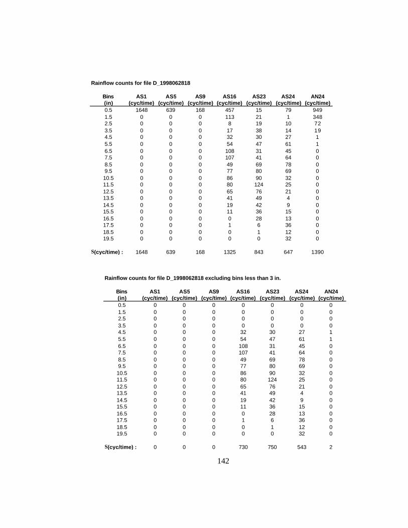
142
Rainflow counts for file D_1998062818
Bins AS1 AS5 AS9 AS16 AS23 AS24 AN24(in) (cyc/time) (cyc/time) (cyc/time) (cyc/time) (cyc/time) (cyc/time) (cyc/time)0.5 1648 639 168 457 15 79 9491.5 0 0 0 113 21 1 3482.5 0 0 0 8 19 10 723.5 0 0 0 17 38 14 194.5 0 0 0 32 30 27 15.5 0 0 0 54 47 61 16.5 0 0 0 108 31 45 07.5 0 0 0 107 41 64 08.5 0 0 0 49 69 78 09.5 0 0 0 77 80 69 010.5 0 0 0 86 90 32 011.5 0 0 0 80 124 25 012.5 0 0 0 65 76 21 013.5 0 0 0 41 49 4 014.5 0 0 0 19 42 9 015.5 0 0 0 11 36 15 016.5 0 0 0 0 28 13 017.5 0 0 0 1 6 36 018.5 0 0 0 0 1 12 019.5 0 0 0 0 0 32 0
Σ(cyc/time) : 1648 639 168 1325 843 647 1390
Rainflow counts for file D_1998062818 excluding bins less than 3 in.
Bins AS1 AS5 AS9 AS16 AS23 AS24 AN24(in) (cyc/time) (cyc/time) (cyc/time) (cyc/time) (cyc/time) (cyc/time) (cyc/time)0.5 0 0 0 0 0 0 01.5 0 0 0 0 0 0 02.5 0 0 0 0 0 0 03.5 0 0 0 0 0 0 04.5 0 0 0 32 30 27 15.5 0 0 0 54 47 61 16.5 0 0 0 108 31 45 07.5 0 0 0 107 41 64 08.5 0 0 0 49 69 78 09.5 0 0 0 77 80 69 010.5 0 0 0 86 90 32 011.5 0 0 0 80 124 25 012.5 0 0 0 65 76 21 013.5 0 0 0 41 49 4 014.5 0 0 0 19 42 9 015.5 0 0 0 11 36 15 016.5 0 0 0 0 28 13 017.5 0 0 0 1 6 36 018.5 0 0 0 0 1 12 019.5 0 0 0 0 0 32 0
Σ(cyc/time) : 0 0 0 730 750 543 2
143
References
ASTM E 1049-85 (1985), “Standard Practices for Cycle Counting in Fatigue Analysis,” American Society for Testing and Materials, West Conshohocken, PA, Reapproved 1999.
Buhl M. (2002), “CRUNCH Users Manual,” National Wind Technology Center at the National Renewable Energy Laboratory, Golden, Colorado
Downing, S. D. and Socie, D. F. (1982), “Simple Rainflow Counting Algorithms,” International Journal of Fatigue, Vol. 4, No. 1, pp. 31-40.
Hudson, D. E. (1979), “Reading and Interpreting Strong Motion Accelerograms,” Earthquake Engineering Research Institute, Engineering Monograph No. 1, Berkeley, CA.
Lamb, J. L. (1985), “Study of Simple Fatigue Resistant Anchorage for Cable-Stayed Applications”, M.S. Thesis, Department of Civil Engineering, The University of Texas at Austin.
Main, J. A. (2000), “Characterization of Rain-Wind Induced Stay-Cable Vibrations from Full-Scale Measurements,” NSF/STA Summer Institute Research Report, Saitama University, Saitama, Japan.
Main, J. A., Jones, N. P., and Yamaguchi, H., (2000), “Characterization of Rain-Wind Induced Stay-Cable Vibrations from Full-Scale Measurements”, Johns Hopkins University, Baltimore, MD and Saitama University, Urawa, Saitama, Japan.
Papailiou, K. O. (1999), “On the Bending of Multi-Layer Strands,” Wire, Vol. 49, No. 5, pp. 44-47.
Paulson, C., Frank, K., and Breen, J. (1983), “A Fatigue Study of Prestressing Strand,” Research Report 300-1, Center for Transportation Research, Bureau of Engineering Research, The University of Texas at Austin, Austin, TX, April 1983.
Poser, Marcel (2001), “Full-Scale Bending Fatigue Tests on Stay Cables”, M.S. Thesis, Department of Civil Engineering, The University of Texas at Austin.

144
Poston, R. W. and Kesner, Keith (1990), “Progress Report Number Two, Evaluation and Repair of Stay-Cable Vibrations, Fred Hartman Bridge, Veterans Memorial Bridge”, Whitlock Dalrymple Poston and Associates, Inc., Manassas, Virginia
PTI Guide Specification (2001), “Recommendations for Stay Cable Design, Testing and Installation”, Post-Tensioning Institute, Phoenix, AZ.
Sarker, P.P., Mehta, K.C., Zhao, Z., (1999), “Aerodynamic Approach to Control Vibrations in Stay-Cables,” Wind Engineering Research Center, Department of Civil Engineering, Texas Tech University, Lubbock, TX.
Timoshenko, S. (1956). "Strength of Materials: Part II - Advanced Theory and Problems," D.Van Nostrand Co., Inc., Princeton, NJ.