CA50 Estimation on HCCI Engine using Engine Speed Variations

Aron Håkansson

1

Acknowledgements First of all I would like to thank all employees, master and PhD students working at the Division of Combustion Engines at LTH. The have all contributed to this thesis by always being helpful to me and by creating a stimulating working environment in general. Furthermore I express my gratitude towards my supervisors Associate Professor Per Tunestål for his valuable support and opinions, PhD Student Hans Aulin & PhD Student Thomas Johansson for their support and cooperation with the engine and measurements. I would like to address special thanks to Richard Backman at GM Powertrain for initiating and letting me carry out this thesis and professor Bengt Johansson for his support and letting me experience the Division of Combustion Engines at LTH. I would also like mention M.Sc. Fredrik Bengtsson who helped me understand his data collection. Special thanks also go to my office colleagues PhD Student Kent Ekholm and PhD student Uwe Horn who have contributed by being helpful and creating a stimulating environment Lund, December 2007 Aron Håkansson

2

Notation α Angular acceleration [rad] β Angle between rod and cylinder axis [rad] θ Crank Angular acceleration [rad/s2] ρ Coefficient of Correlation [-] φ Crank Angle [rad] ω Crank Angular velocity [rad/s] Ji Mass moments of inertia of body i [kgm2] fsampling Sampling frequency [Hz] Nrpm Engine speed stated in rpm [rpm] rencoder Encoder resolution [°] e Sampling error [%] A/D Analog to Digital ATDC After Top Dead Center C(X, Y) Covariation between Stochastic variable X and Y. [-] CA50 Crank Angle for 50% heat release ATDC [°] CAD Crank Angle Degree [°] D(X, Y) Standard deviation between Stochastic variable X and Y. [-] HCCI Homogeneous Charge Compression Ignition IMEP Indicated Mean Effective Pressure (here net) [bar] RPM Revolutions Per Minute TDC Top Dead Center

3

CONTENTS ACKNOWLEDGEMENTS ......................................................................................................................... 1 NOTATION .................................................................................................................................................. 2 ABSTRACT .................................................................................................................................................. 5

1.1 BACKGROUND ..................................................................................................................................... 6 1.1.1 HCCI Engine............................................................................................................................... 6

1.2 PURPOSE AND GOAL ............................................................................................................................ 7 1.3 OUTLINE .............................................................................................................................................. 7 1.4 TEST SETUP .......................................................................................................................................... 8

1.4.1 Data Acquisition Board ............................................................................................................... 8 1.4.2 Crank Angle Encoder ................................................................................................................. 8 1.4.3 Cylinder Pressure Sensors .......................................................................................................... 8 1.4.4 Electric Brake .............................................................................................................................. 9

1.5 HEAT RELEASE AND CA50 ................................................................................................................. 9 2. METHODS .............................................................................................................................................. 11

2.1 ION CURRENT SENSING ..................................................................................................................... 11 2.2 KNOCK SENSOR MEASUREMENTS .................................................................................................... 11 2.3 ENGINE SPEED ................................................................................................................................... 11

2.3.1 Energy model............................................................................................................................. 11 2.3.2 Mechanical Model ..................................................................................................................... 13 2.3.3 Working principle ..................................................................................................................... 16

2.4 EVALUATION OF METHOD ................................................................................................................ 18 2.4.1 Correlation Coefficient ............................................................................................................. 18 2.4.2 Cycle to Cycle Characteristics ................................................................................................... 19 2.4.3 Parameter influence on Correlation Coefficient ...................................................................... 20 2.4.4 Parameter influence on CAD offset ......................................................................................... 20 2.4.5 CAD offset and Correlation Coefficient ................................................................................... 21 2.4.6 Linear Behavior ........................................................................................................................ 23

3. RESULTS ................................................................................................................................................ 24 3.1 MODEL ENGINE IN HCCI MODE ....................................................................................................... 24

3.1.1 Operating point 2500 rpm 4.1 bar IMEP ................................................................................. 24 3.1.2 Summary of all operating points .............................................................................................. 25

3.2 MODEL ENGINE IN OTTO MODE ....................................................................................................... 26 3.2.1 Operating point 1500 rpm and 2.5 bar IMEP .......................................................................... 26 3.2.2 Summary of all operating points .............................................................................................. 27

3.3 HCCI ENGINE EXPERIMENTS ........................................................................................................... 28 3.3.1 Operating point 1525 rpm and 4.5 bar IMEP .......................................................................... 28 3.3.2 Operating point 2527 rpm and 4.1 bar IMEP .......................................................................... 31 3.3.3 Summary of all operating points .............................................................................................. 34

3.4 OTTO-ENGINE .................................................................................................................................... 35 3.4.1 Test Cell Measurements Summary ........................................................................................... 35

4. DISCUSSION .......................................................................................................................................... 36 4.1 POSSIBLE SOURCES OF ERROR ......................................................................................................... 36

4.1.1 Deviation from Rigid Body Behavior ....................................................................................... 36 4.1.2 Variations in Brake Torque ...................................................................................................... 38 4.1.3 Measurement Equipment Limitations ...................................................................................... 39 4.1.4 Influence of Hardy Disc ............................................................................................................ 39 4.1.5 Engine Imperfections ................................................................................................................ 39 4.1.6 Influence of Control Method .................................................................................................... 39 4.1.7 Deviation of geometric parameters ........................................................................................... 40

4

4.2 MODEL ENGINE RESULTS ................................................................................................................. 41 4.3 HCCI ENGINE RESULTS ................................................................................................................... 41 4.4 OTTO ENGINE RESULTS ..................................................................................................................... 42

5. CONCLUSION ....................................................................................................................................... 43 6. FUTURE WORK.................................................................................................................................... 44

6.1 IMPROVING SIGNAL/NOISE RATIO ................................................................................................... 44 6.2 ENGINE IN VEHICLE ANALYSIS ........................................................................................................ 44 6.3 FREQUENCY ANALYSIS ..................................................................................................................... 44

APPENDIX: ................................................................................................................................................ 45 ENGINE SPECIFICATIONS ........................................................................................................................ 45 ENERGY MODEL ...................................................................................................................................... 45

REFERENCES ........................................................................................................................................... 46

5

Abstract This thesis is about estimation of CA50 from engine speed variations on a HCCI engine. The HCCI (Homogeneous Charge Compression Ignition) engine concept requires a combustion control system operating on a cycle to cycle basis. The prevailing method of achieving this control is based upon the combustion parameter CA50. CA50 describes the crank angle at which 50 % of the heat from combustion has been released. The dominating technique of receiving this parameter is from the use of pressure sensors. The disadvantages with these sensors are that the technique is not yet mature for mass production from a cost and reliability perspective. The search for other methods of receiving combustion feedback is therefore of interest. Focus has been directed to other, indirect, methods of estimating CA50. This thesis evaluates a method using variations in engine speed for the purpose of estimating CA50. The method’s working principle is founded on the expected variations in engine speed increase that occurs due to different combustion phasing. The method is evaluated on a four cylinder turbocharged 2.2 litre GM HCCI engine. The result reveals that this method’s accuracy even though it is showing high correlations under favorable conditions does not cover a wide load range with preserved accuracy and robustness and thereby does not meet the high demands that are needed for this vital control parameter. Keywords: HCCI control, CA50 estimation, Indirect Methods, Engine Speed Variations

6

1. Introduction 1.1 Background 1.1.1 HCCI Engine Modern cars are currently experiencing increasing demands concerning fuel efficiency and low emissions from both consumers and governments. The two dominating engine concepts on the market today are the Diesel- and Otto principles. A comparison between the two engines show that the Otto engine equipped with a catalytic converter provides low emissions but lacks in efficiency. The Diesel engine on the other hand provides high efficiency but also produces high emissions of NOx and particles. An engine concept capable of combining the efficiency of a diesel engine with the emissions levels of an Otto engine is the HCCI engine (Homogeneous Charge Compression Ignition).

Figure 1: Diesel, Otto and HCCI combustion principles, adapted from New Scientist Magazine (January 2006) The HCCI engine is highly sensitive to variations in parameters that have an influence on the combustion. A temperature variation less than 5 degrees Celsius could be sufficient for the combustion to go from too early to too late and possibly no combustion at all. To be able to work properly the HCCI engine needs an active combustion control system based on feedback on a cycle to cycle basis, see [1] p.624. To be able to fulfill this feedback pressure sensors, mounted in the cylinder head, are currently used in laboratory environments. Pressure sensors have the disadvantage of being expensive and furthermore contribute to an increased level of complexity and possible sources of error.

7

1.2 Purpose and Goal The purpose of this master thesis is to estimate the combustion parameter CA50 based on already existing sensors on the engine. This indirect method should, if successful, be utilized in the feedback control system of the combustion. The basic idea is to make use of the crankshaft angular position sensor for determination of the crankshaft acceleration. Other possible indirect methods are ion current measurement with the spark plugs and vibration analysis based on the knock sensor signal. If possible it should also be investigated what crank angle resolution is needed for the estimation of CA50. Initially the maximum available resolution of 0.2 CAD is used. Ideally, however, a resolution of only 6 CAD for the speed sensor would be preferred. Another interesting topic is to decide the load range for which each method is suitable. Perhaps a combination of methods is applicable and required. 1.3 Outline This thesis consists of a significant share of experimental work. Measurements have been performed and the collected data have been studied and analyzed in a MATLAB environment. The measurements were carried out on a four cylinder turbocharged 2.2 litre GM HCCI engine. The engine is placed in a test cell at the division of combustion engines at Lund University. The procedure includes gathering and analysis of measurement data for a variety of different engine speed and load cases. Data from the master thesis Estimation of Indicated and Load Torque from Engine Speed Variations [2] by Fredrik Bengtsson is to some extent used for verification of the presented method. This data is from a four cylinder turbocharged Otto engine.

8

1.4 Test setup A schematic view of the test cell setup is shown in Figure 2 below.

Figure 2: Schematic Test Cell Setup 1.4.1 Data Acquisition Board The pressure signals and crank angle position were collected using a DAP5400a Data Acquisition Board from Microstar Laboratories. The DAP5400a board is capable of eight A/D conversions simultaneously with a resolution of 14 bit at a sampling frequency of 1.25 MHz. 1.4.2 Crank Angle Encoder The crankshaft position was measured using a Leine & Linde 520 sensor. The sensor is located at the free end of the crankshaft. It produces a binary signal from 0 to 5V every 0.2°. This resolution results in 1800 pulses per revolution and 3600 pulses per engine cycle. 1.4.3 Cylinder Pressure Sensors The cylinder pressure was measured using four Kistler-6043Asp pressure sensors. The signals from the pressure sensors were transformed and amplified using a Kistler Multichannel Charge Amplifier type 5011B. The Charge Amplifier converts the electric charge induced in the pressure sensor into a voltage proportional to the pressure in the cylinder. This voltage is measured by the DAP5400a board which converts the voltage level into data bits, stored in the log file of the current measurement session.

9

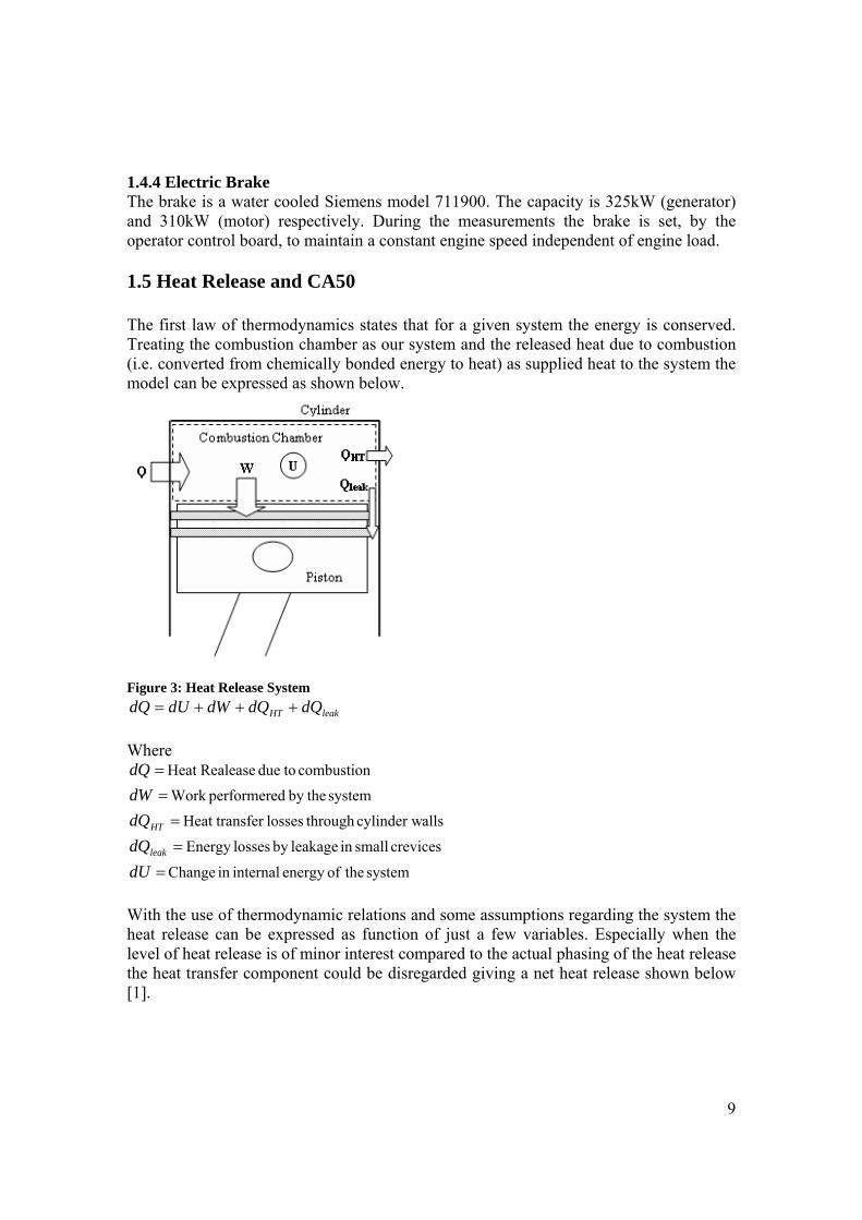
1.4.4 Electric Brake The brake is a water cooled Siemens model 711900. The capacity is 325kW (generator) and 310kW (motor) respectively. During the measurements the brake is set, by the operator control board, to maintain a constant engine speed independent of engine load. 1.5 Heat Release and CA50 The first law of thermodynamics states that for a given system the energy is conserved. Treating the combustion chamber as our system and the released heat due to combustion (i.e. converted from chemically bonded energy to heat) as supplied heat to the system the model can be expressed as shown below.

Figure 3: Heat Release System

leakHT dQdQdWdUdQ +++= Where

systemtheofenergyinternalinChange

crevicessmallinleakagebylossesEnergy

allscylinder wthroughlossestransferHeatsystemthebydperformereWork

combustion todueRealeaseHeat

===

==

dUdQdQdWdQ

leak

HT

With the use of thermodynamic relations and some assumptions regarding the system the heat release can be expressed as function of just a few variables. Especially when the level of heat release is of minor interest compared to the actual phasing of the heat release the heat transfer component could be disregarded giving a net heat release shown below [1].

10

VdppdVdQ1

11 −

+−

=γγ

γ

chambercombustiontheingasmixturetheofpropertymicthermodyna

chambercombustioninPressurevolumechamberCombustion

==

==

v

p

CC

pV

λ

Taking the heat release function above calculated from measured data from the engine and then plotting the accumulated heat release during a section in the region of the TDC position of the combustion stroke will create a typical appearance of the cumulative heat release shown below. The position where the accumulated heat release reaches 50% of the total released heat is called CA50 which is the parameter that is of interest in this study.

Figure 4: Definition of CA50

11

2. Methods 2.1 Ion Current Sensing The ion sensing technique is in modern engine control systems used as a knock and misfire detection system. The ion sense system is based around the spark plug and suitable measurement electronics. The working principle is to apply a voltage, after the spark has been fired, to the spark plug and then measure the current trough the measurement circuit. The current is dependent on the amount of free charges produced during the combustion. In the thesis Ion Current and Torque Modeling for Combustion Engine Control [3] engine parameters such as peak pressure and start of combustion are mentioned as other information that has been extracted from ion current measurements. 2.2 Knock Sensor Measurements The knock sensor is an accelerometer based upon a piezoelectric or piezoresistive crystal. A piezoelectric crystal induces a charge when exposed to movement i.e. vibrations of the engine block. The charge is converted to a voltage by circuitry inside the knock sensor. A piezoresistive crystal responds to vibrations by changing its resistance. Knocking is from an engine perspective a harmful state caused by self ignition of the fuel air mixture in the cylinder. Knocking causes high-amplitude pressure oscillation inside the combustion chamber which can be detected using the knock sensor. In the SAE paper titled In-Cylinder Pressure Estimation from Structure-Born Sound [4] a model for estimation cylinder pressure is proposed based on measurements on a spark ignited four cylinder engine equipped with four accelerometers. 2.3 Engine Speed 2.3.1 Energy model The basic idea behind extracting the combustion phasing, i.e. CA50 from the engine speed variations is described trough a simplified model. The engine is here treated as a rotating shaft at an average angular velocity ω with a moment of inertia given by Jengine. Due to the combustion there is an applied torque defined as Min and a corresponding braking torque from the dyno Mout.

12

Figure 5: Torque equilibrium of a rotating rigid body

Equilibration for the system gives us an expression for the angular acceleration α

( ) ( ) ( )

( ) ( )( )

( )( )ϕϕ

ϕϕϕα

ωααϕϕϕ

engineengine

outin

engineoutin

JM

JMM

dtdJMM

Δ=

−=

=⋅=− ,

The average torque delivered from the engine to the dyno during a full engine cycle is under normal operating conditions assumed to be constant from cycle to cycle.

( )out

out

averagedyno MconstdM

M ≈≈=∫

.4

4

0, π

ϕϕπ

To maintain a constant average operating speed of the engine the dyno control system is assumed to apply this average torque to the engine. Considering this applied torque to be constant rules out the effect of the dyno control system of the model1. This will leave the engine speed variations as function of the applied torque due to the combustion. The hypothesis of this method is that the angular acceleration α and the corresponding increase in engine speed thereby will be dependent on the phasing of the applied torque from the combustion. The torque phasing and duration is then assumed to be related to the combustion phasing, CA50.

1 A rapid dyno control system would cancel out all speed variations by adjusting the brake torque to maintain the constant angular velocity, set by the operator.

13

2.3.2 Mechanical Model The combustion engine will, due to its reciprocating nature, cause a fluctuating speed and acceleration of its moving internal parts. The piston as an example will vary its linear velocity between zero and up to 1.5 times the mean piston speed during one stroke (180° turn of crankshaft) of the engine. The masses of these components will according too Newton’s law

maF =

create oscillating forces acting on the crankshaft. In addition to the mass forces the driving force from the pressure generated by the combustion will also contribute to the oscillation since both the pressure acting on the piston and the leverage on the crankshaft will vary during a cycle. With the knowledge of the geometry and mass of the crank mechanism of the engine it is possible to create a basic mechanical model, consisting of rigid bodies, of the engine at hand. Figure 6 shows gas forces acting on a crank mechanism and Figure 7 shows a geometrical model of the crank mechanism.

Figure 6: Forces acting on a crankshaft mechanism, Förbränningsmotorer, Johansson

14

Figure 7: Geometrical crankshaft mechanism, Förbränningsmotorer, Johansson Starting from these models one could derive an expression for the torque acting on the crankshaft (for the full derivation consult [1] chapter 12). The resulting torque acting on the crankshaft will consist of terms from gas forces, mass forces and forces from friction according to

frictionmassgascrank MMMM ++=

where the average torque from mass forces during a full engine cycle will be zero but, dependent on engine speed, instantaneously will create a significant torque acting on the crank. Figure 8 shows the torque variation during a series of cycles created from the actual pressure trace with data from a test cell run at 1500 rpm and 120Nm (data from Estimation of … F. Bengtsson [2]).

Figure 8: Torque variations in mechanical model based on measured pressure trace

15

These torque variations will create a variation in engine speed according to the torque equilibrium

brakeengine

crank

JM

+

=α

with the assumption that the brake torque and moment of inertia are constant a synthetic engine speed could be expressed as

∫+

−+= dt

JMM

brakeengine

brakecrank0ωω

where ω0 is the speed at time zero (in this case set to the set point speed of the brake) Figure 9 below shows the engine speed variations during a motored run from a measured speed signal and the speed variation based on the mechanical model computed from the pressure trace from the same measured run.

Figure 9: Measured and computed engine speed variations, motored run at 1500 rpm

16

2.3.3 Working principle The working principle of extracting CA50 estimation starts by looking at a section of engine speed variations close to the top dead center for each cylinder at its combustion stroke. See Figure 10.

Figure 10: Engine speed variations with Top Dead Centers, TDC, circled.

17

Figure 11: Working principle of CA50 estimation. The idea based upon the physical model is that there will be an increase in engine speed from the torque applied due to the combustion and that the timing of this engine speed increase will vary due to the combustion phasing, i.e. CA50. For this reason an algorithm consisting of the following steps was created:

1) Establish a suitable engine speed increase, the “threshold rpm”. 2) Select a position near TDC as a reference point. 3) Start to measure the engine speed difference between the reference point

engine speed and the actual engine speed by moving in a positive direction (increasing crank angle) until the difference matches the “threshold rpm”.

4) Estimate CA50 by the position of where the threshold rpm is reached.

18

2.4 Evaluation of Method 2.4.1 Correlation Coefficient The reference point and the threshold rpm are adjusted to give the best possible correlation between the estimated CA50 and the indicated (measured by pressure signals) CA50 for each cylinder, load and engine speed during a measurement (about 30 engine cycles). The correlation coefficient defined by

( ) ( )( ) ( )YDXD

YXCYX ,, =ρ

is used as a performance measure. The correlation coefficient does not depend on the amplitudes (different from zero) of the compared signals. Figure 12 shows correlation coefficients between various sine based functions to illuminate that the amplitude has no influence. In this thesis the coefficient of correlation will be abbreviated with one of the following expressions, “c.o.c”, “Corr” or “CorrCoeff”.

Figure 12: Correlation coefficients between different functions

19

2.4.2 Cycle to Cycle Characteristics Figure 13 shows how the indicated CA50 (blue line) varies from cycle to cycle. The red line shows how the estimated CA50 varies for the same cycles. The correlation coefficient between the two lines is named “Corr” and is in this case equal to 0.85. For each cycle there is a significant deviation between the indicated and estimated CA50. The average deviation for all cycles is calculated and is named “CAD offset”. If the estimated CA50 is adjusted for this offset the result looks like the one displayed in Figure 14. In the following results the estimated CA50 is adjusted the same manner. Figures represents operating point 1525 rpm and 4.5 bar IMEP.

Figure 13: Cycle to Cycle variations in indicated (blue) and estimated (red) CA50

Figure 14: Cycle to Cycle variations in indicated (blue) and estimated (red) CA50 with offset correction.

20

2.4.3 Parameter influence on Correlation Coefficient When varying the two parameters in the method the combination of these two will result in a corresponding correlation coefficient. Figure 15 displays what effect the setting of the two parameters has on the correlation coefficient at operating point 1525 rpm and 4.5 bar IMEP. The diagonal ridge like shape of the figure is a consequence of the working principle of the method.

Figure 15: Coefficient of correlation variation due to varying parameter settings, blue line indicates highest c.o.c. 2.4.4 Parameter influence on CAD offset Figure 16 displays how the CAD offset varies with the parameter settings. Typically the CAD offset increases with increased RPM threshold since a high RPM threshold is reached at a CAD position further away from TDC and hereby increasing the CAD offset.

Figure 16: CAD offset variation due to varying parameter settings, blue line indicates highest c.o.c.

21

2.4.5 CAD offset and Correlation Coefficient The correlation coefficient is calculated over a wide range of settings of the threshold and reference point variables. For each individual setting there is a corresponding correlation coefficient and related offset. Plotting the correlation coefficient and the offset together gives a sense of how suitable the CA50 estimation method is for the particular cylinder. Figure 17 displays the result of Cylinder 1 when the engine is operated at 1500 rpm and 4.5 bar IMEP. Figure 18 shows the behavior of the mechanical model engine being simulated to run with the pressure trace from the real engine at the same operating point. The results reveal that the model engine produces high correlations for a much wider range of parameter setting compared to the real engine. The CAD offset are however somewhat similar for the offset corresponding to the top correlations.

Figure 17: Displaying CAD offset and coefficient of correlation for the HCCI engine

22

Figure 18: CAD offset and correlation coefficient for the model engine running in HCCI mode

23

2.4.6 Linear Behavior The linear behavior in the relation between indicated and estimated CA50 is displayed in Figure 19, operating point 1525 rpm and 4.5 bar IMEP. The blue line represents straight line least squares fit between indicated and estimated CA50. The slope, k, represents the relationship between the changes of indicated CA50 and the corresponding changes of estimated CA50.

Figure 19: Linearity between indicated and estimated CA50

24

3. Results 3.1 Model Engine in HCCI mode 3.1.1 Operating point 2500 rpm 4.1 bar IMEP Figure 20 displays results from running the model engine with the measured pressure trace from the HCCI engine at 4.1 bar IMEP and 2500 rpm.

Figure 20: Model engine running in HCCI mode at 4.1 bar IMEP at 2500 rpm. Plots show Cylinder 1 (left) and Cylinder 3 (right).

25

3.1.2 Summary of all operating points In the following two figures the coefficient of correlation and CAD offset is displayed. The results indicate that the method of estimating CA50 presented here correlates well with indicated CA50. Figure 21 displays the correlation coefficient and Figure 22 the CAD offset for different operating points. Each circle represents the average value for all cylinders.

Coefficent of Correlation Average

0,99

0,98

0,97

0,990,99 0,99

0,990,99

0,95

0,960,98

2,5

3

3,5

4

4,5

5

1250 1500 1750 2000 2250 2500 2750

Speed [rpm]

Load

[bar

]

0,990,980,970,990,990,990,990,990,950,960,98

Figure 21: Correlation coefficient for the model engine running in HCCI mode for all operating points. Values represent averages for all cylinders.

CAD offset Average

5,0

4,5

4,3

4,04,5 4,5

4,04,5

5,0

5,05,0

2,5

3

3,5

4

4,5

5

1250 1500 1750 2000 2250 2500 2750

Speed [rpm]

Load

[bar

]

5,04,54,34,04,54,54,04,55,05,05,0

Figure 22: CAD offset for the model engine running in HCCI mode for all operating points. Values represent averages for all cylinders.

26

3.2 Model Engine in Otto mode 3.2.1 Operating point 1500 rpm and 2.5 bar IMEP Figure 23 displays results from running the model engine a test bench pressure trace from the Otto engine at 2.5 bar IMEP and 1500 rpm. Note that the slope, k, is almost twice the value received with a pressure trace from HCCI combustion. This is probably due to the fact that the actual system consisting of engine, brake and accompanying transmission is flexible. This is not further studied however.

Figure 23: Model engine running in Otto mode at 4.1 bar IMEP and 2500 rpm. Plots show Cylinder 1 (left) and Cylinder 3 (right). Lower figure: Estimated CA50 (red line) and indicated CA50 (blue line).

27

3.2.2 Summary of all operating points Figure 24 and Figure 25 show the correlation coefficients and CAD offsets are, respectively, for various operating points. The results indicate that the method of estimating CA50 presented here correlates well with indicated CA50. Each circle represents the average value for all cylinders. There is a large amount of data from measurements on the Otto engine. The result presented here is just to give a load range overview.

Coefficent of Correlation Average

0,98

0,99

0,99

0,98

1

3

5

7

9

11

1250 1500 1750 2000 2250 2500 2750

Speed [rpm]

Load

[bar

] 0,980,990,990,98

Figure 24: Correlation coefficients for the model engine running in Otto mode for all operating points. Values represent averages for all cylinders.

CAD Offset Average

10,0

10,0

10,0

10,0

1

3

5

7

9

11

1250 1500 1750 2000 2250 2500 2750

Speed [rpm]

Load

[bar

] 10,010,010,010,0

Figure 25: CAD offsets for the model engine running in Otto mode for all operating points. Values represent averages for all cylinders.

28

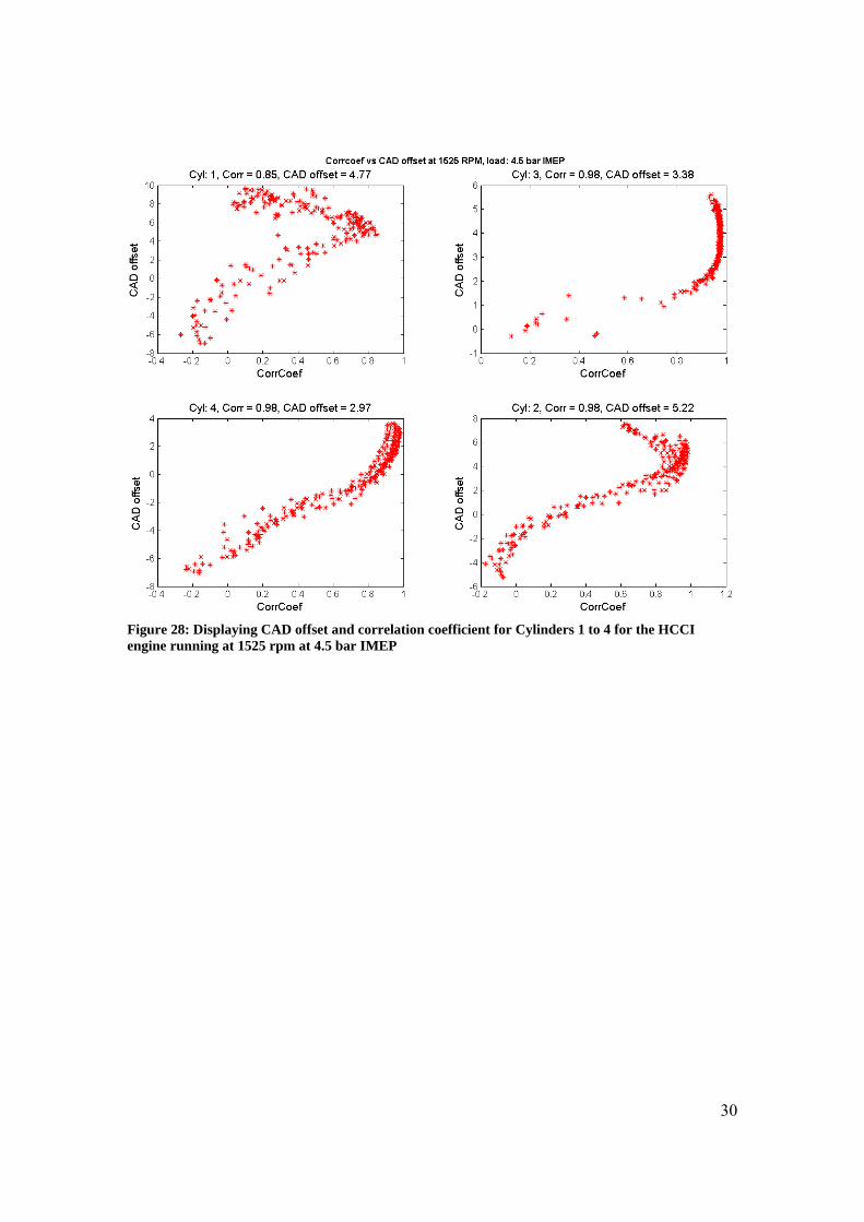
3.3 HCCI Engine experiments 3.3.1 Operating point 1525 rpm and 4.5 bar IMEP Figures 26-28 display the result from an operating point giving high correlation between indicated and estimated CA50.

Figure 26: Estimated CA50 (red line) and indicated CA50 (blue line) for 30 consecutive cycles on Cylinders 1 to 4. HCCI engine running at 1525 rpm and 4.5 bar IMEP.

29

Figure 27: Linear relation between the estimated and indicated CA50 for Cylinders 1 to 4. HCCI engine running at 1525 rpm and 4.5 bar IMEP.

30

Figure 28: Displaying CAD offset and correlation coefficient for Cylinders 1 to 4 for the HCCI engine running at 1525 rpm at 4.5 bar IMEP

31

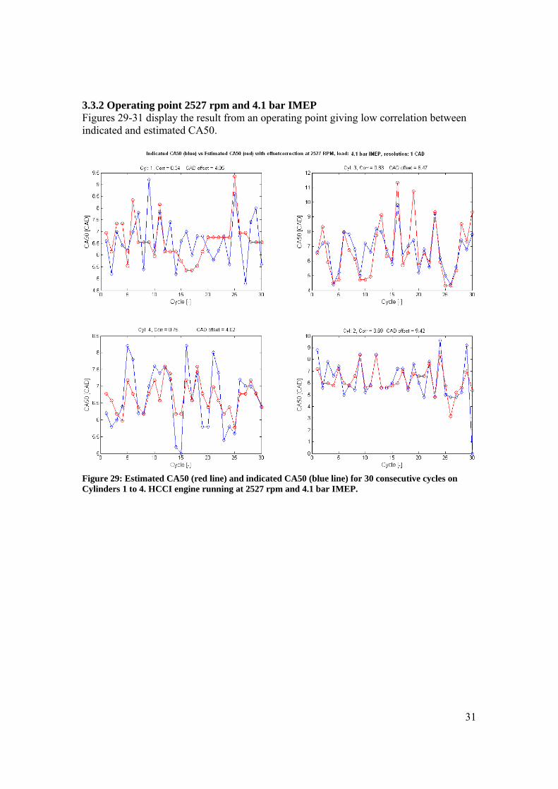
3.3.2 Operating point 2527 rpm and 4.1 bar IMEP Figures 29-31 display the result from an operating point giving low correlation between indicated and estimated CA50.

Figure 29: Estimated CA50 (red line) and indicated CA50 (blue line) for 30 consecutive cycles on Cylinders 1 to 4. HCCI engine running at 2527 rpm and 4.1 bar IMEP.

32

Figure 30: Linear relation between the estimated and indicated CA50 for Cylinders 1 to 4. HCCI engine running at 2527 rpm and 4.1 bar IMEP.

33

Figure 31: CAD offset and correlation coefficient for Cylinders 1 to 4 for the HCCI engine running at 2527 rpm at 4.1 bar IMEP

34

3.3.3 Summary of all operating points In the following two figures the coefficient of correlation and CAD offset are displayed. Figure 32 displays the correlation coefficient and Figure 33 the CAD offset for various operating points. Each circle represents the average value for all cylinders.

Coefficent of Correlation Average

0,65

0,88

0,83

0,760,93 0,77

0,700,95

0,47

0,520,72

2,5

3

3,5

4

4,5

5

1250 1500 1750 2000 2250 2500 2750

Speed [rpm]

Load

[bar

]

0,650,880,830,760,930,770,700,950,000,470,520,72

Figure 32: Correlation coefficients for the HCCI engine for all operating points. Values represent averages for all cylinders.

CAD Offset Average

6

5

5

34 4

56

6

66

2,5

3

3,5

4

4,5

5

1250 1500 1750 2000 2250 2500 2750

Speed [rpm]

Load

[bar

]

65534456

666

Figure 33: CAD offsets for the HCCI engine for all operating points. Values represent averages for all cylinders.

35

3.4 Otto-engine 3.4.1 Test Cell Measurements Summary In the following two figures the correlation coefficient and CAD offset are displayed. Figure 34 displays the correlation coefficient and Figure 35 the CAD offset for various operating points. Each circle represents the average value for all cylinders. The correlation is generally very low. The value of the CAD offset is however similar to the value of the mechanical model engine running in Otto mode (Figure 25, Section 3.2.2).

Coefficent of Correlation Average

0,28

0,54

0,40

0,46

1

4

7

10

1250 1500 1750 2000 2250 2500 2750

Speed [rpm]

Load

[bar

] 0,280,540,400,46

Figure 34: Correlation coefficient for the Otto engine for all operating points. Values represent averages for all cylinders.

CAD Offset Average

10,0

11,5

9,9

10,0

1

3

5

7

9

11

1250 1500 1750 2000 2250 2500 2750

Speed [rpm]

Load

[bar

] 10,011,59,910,0

Figure 35: CAD offset for the HCCI engine for all operating points. Values represent averages for all cylinders.

36

4. Discussion 4.1 Possible Sources of Error 4.1.1 Deviation from Rigid Body Behavior The method of CA50 estimation from engine speed variations presented here is simple in nature and shows good results for a basic mechanical engine model. Using the same method for CA50 estimation on a real engine will only produce good results for a narrow operating range. The reasons for this could be several and in this chapter the ones that are believed to have the greatest impacts on the results will be discussed. Figure 36 shows the engine speed variations at 2072 rpm and 4.3 bar IMEP. It is obvious that the real engine variations do not behave like the ones from the basic mechanical model consisting of interconnected rigid bodies. In Figure 37 the speed variation is shown for an operating point of 2527 rpm and 4 bar IMEP.

Figure 36: Measured and modeled engine speed variations at 4.3 bar IMEP and 2072 rpm

37

Figure 37: Measured and modeled engine speed variations at 4.0 bar IMEP and 2527 rpm (crank angle resolution: 6 CAD) The above figures indicate that the real engine speed variation is more complex than can be described by a basic mechanical model. For example the influence of the torque variations from driving the balance shafts and camshafts is not considered in the model but could influence the real results.

38

4.1.2 Variations in Brake Torque Even though one could find a dynamic model fully describing the engine speed variations the impact from the load torque from the brake is not considered. In the engine model this torque is assumed to be constant. When the brake is adjusting its load torque it is also effecting the engine speed variations. Figure 38 shows how the engine model suddenly drops in speed due to a torque decrease caused by misfiring in one of the cylinders, this is however barely noticeable in the measured engine speed variation since the control system of the brake is active. The impact from the continuous speed control on the engine speed variations is unknown.

Figure 38: Misfire at cylinder 3 halfway into a measurement cycle. The black line shows the expected speed drop if the brake torque would be constant. The red line shows the actual measured engine speed. Measurement at 2.9 bar IMEP and 1500 rpm

39

4.1.3 Measurement Equipment Limitations The DAP 5400a data acquisition board has a maximum sampling frequency of 1.25MHz. Depending on the selected resolution of the crank angle decoding and the engine speed this will create a typical maximum error e. This error in percent could approximately be described as

samplingencoder

rpm

frN

e⋅

⋅=

600

For a resolution of 0.2 CAD the error becomes 3.6 % at 1500 rpm and 0.12 % at resolution of 6 CAD. In the result presented in the previous chapter the resolution is set to 1 CAD giving a maximum error of 0.7 %. The calculated speed is then filtered through a moving average filter ranging over 6 CAD. Since calculation of engine speed only needs a binary signal from the crank angle encoder a separate time based system could be used for the engine speed signal measurement. Additional sources of error could occur in the pressure transducers with accompanying amplification. 4.1.4 Influence of Hardy Disc The Hardy Disc connects the brake with the crankshaft and is supposed to create a softer connection between the engine and the brake. This soft connection will have an influence on the engine speed variations. The magnitude of this influence is however unknown. An unfavorable situation would result in a flexibility of the connection that depends on the crank position. The high frequency variations that appear in the engine speed could thus originate not only from the engine flexing but also from the flexing in the Hardy disc. 4.1.5 Engine Imperfections During later research carried out on the HCCI engine the piston in cylinder 1 broke down. It can not be ruled out that there existed a previous damage on this piston affecting the results. 4.1.6 Influence of Control Method The charge temperature is controlled using a technique called NVO (Negative Valve Overlap). The working principle of this method is to use an adjustable amount of hot residual gases from the combustion as a heat source. By varying the amount of residual gases in the cylinder the temperature conditions will also be affected. Hereby it is possible to control the combustion timing. The residual volume is controlled using variable camshaft timing during the exhaust stroke. In the engine configuration studied the residual gases will be compressed and expanded simultaneously with a cylinder in its compression and working stroke, see Figure 39 . This implies that the engine speed variation is caused not just by the actual CA50 at the cylinder studied but also dependent on the previous CA50 at the parallel cylinder.

40

Figure 39: Figure showing pressure traces for all cylinders. Note that there is two pressure peaks occurring every 180 degrees. Note the lower pressure occurring due to the NVO and the top pressure due to combustion. 4.1.7 Deviation of geometric parameters Due to erroneous in geometric parameter value in the analysis the calculation of indicated CA50 deviates from the correct value. The error is caused by this deviation is however small, see Figure 40.

Figure 40: Figure showing CA50 calculations based on correct and incorrect geometrical parameters. The difference varies between 0 – 0.2 degrees.

41

4.2 Model Engine Results The hypothesis of the method presented in this thesis was that the variation in combustion phasing results in a corresponding variation in speed increase phasing. The engine model indicates that this relation exists under ideal circumstances. Since it is a “mathematical” model one could ask oneself the question why the correlation is less than 100%. A likely reason is that the threshold and reference point variables are only varied in increments of 1 CAD and 1 rpm respectively in the numerical analysis and thereby not finding the optimal setting. 4.3 HCCI Engine Results The results from applying the CA50 estimation method presented here show that it could detect variations in CA50 within a narrow operating range. The correlation coefficient seems to decrease during (see Figure 32 section 3.3.3) decreased load and/or increased engine speed. The nature of this behavior could be explained by just considering the energy ratio between the energy supplied from the combustion and the energy of the rotating engine. It could also be understood knowing that the mass forces (from the oscillating engine parts) increase as the square of the engine speed. The gas forces will thereby rapidly decrease its chances of influencing the engine speed variations. Figure 41 displays a principal model (see appendix for derivation) of how the engine speed increase would vary depending on supplied energy and operating speed. The model just considers the engine as a homogeneous rigid body but clearly illustrates the principal nature of the problem.

Figure 41: Illustrating the nature of how the engine speed increase drops due to increased speed and/or decreased load.

42

4.4 Otto engine results The results from applying the CA50 estimation method presented here show that it can not detect variations in CA50 during Otto engine measurements. Since simulations with pressure traces from the Otto engine measurements show very good results this outcome is, at first, surprising. The reason for the poor result can perhaps be seen in Figure 42 below. The figure shows the engine speed variations during similar operating points (1500 rpm and 4.5 bar IMEP) for both engine types. The basic engine geometry is equal except for a higher compression ratio in the HCCI engine.

Figure 42: Engine speed variations from HCCI engine (blue line) and Otto engine (green line) with equal load, 4.5 bar IMEP, and speed, 1500rpm. The engines have been tested at different locations.

43

5. Conclusion The method of estimating CA50 presented here does not fulfill the robustness and accuracy one should demand when it comes to such a vital control function as estimating CA50 for mass production applications. The failure of this model could perhaps be explained by its simplicity. The underlying problem when it comes to analyzing engine speed variations is that there are several, perhaps too many, variables that affect the engine speed variations e.g. load, speed and inertia. The complexity behind the resulting engine speed variations should be possible to describe with the right model, but the computational effort and robustness requirements might still not be met. One major drawback with estimating CA50 from engine speed variations is that the engine speed will vary even though there is no combustion. The method presented here would not detect a misfire in such an obvious way that a pressure transducer would. Still the method presented here could be of some value perhaps as a complementary method or for diagnosis in a future application.

44

6. Future Work 6.1 Improving Signal/Noise Ratio Basically it is all about extracting the pressure signal from the engine speed variation. One could consider all the factors, except the pressure, influencing the speed variation as noise. If this noise could be reduced the useful signal from the pressure could be better analyzed. One way to do this is to reduce the actual speed variation with the expected speed signal from a cycle without the combustion, this requires an accurate model. Another method suggested by the author has been to subtract the engine speed behavior before TDC from the engine speed behavior after TDC leaving the signal from pressure and friction left to analyze. A third suggested method could be to filter out the natural frequency caused by the torsion movements in the crank shaft. 6.2 Engine in Vehicle Analysis The environment in a test cell differs in many ways from the one in an actual vehicle. Regarding engine speed variations the obvious difference is the effect of the transmission flex and inertia compared to the one existing in a test cell with a large brake. The effect that this different boundary condition has on the engine speed variations is of interest. 6.3 Frequency Analysis Previous successful studies have been carried out using frequency analysis with FFT techniques for estimation of crankshaft torque. Frequency analysis requires a higher precision in the data acquisition system than the one used in this study. A time based data acquisition system is suggested for this purpose.

45

Appendix: Engine Specifications Table 1: Engine specifications. Engine Type Four cylinder in line, turbocharged HCCI Cylinder Head 16 valve DOHC Bore × Stroke 86 × 94.6 [mm] Displacement Volume 2.198 [L] Compression ratio 11.75 Connecting rod length 145.5 [mm] Firing order 1-3-4-2 Fuel Type unleaded 95 Piston mass (including bolt and rings) 457 [g] Connecting rod mass 640 [g] Connecting rod mass center 42 [mm] (from big end center) Energy model

limittheatzerobecomesdifferenceThe0limcombustionbeforeandafterspeedtheComparing

combustionafterspeedenginetheSolving

combustionafterlevelEnergyidleengineatexistinglevelenergytheto

factor withrelated,combustionfromsuppliedlevelEnergy

combustionbeforelevelEnergy

1

120

2113

20

213

20

21

23

213

2002

211

=Δ

−+=−=Δ

+=⇒

⋅⋅+⋅=⋅

+=

⋅⋅=⋅=

⋅=

∞→ω

ωδωωωωω

δωωω

ωδωω

δωδ

ω

ω

JJJ

EEE

JEkE

JE

46

References [1] Bengt Johansson, Förbränningsmotorer, Lecture material from: Department of Energy Sciences, Division of Combustion Engines, Lund Institute of Technology 2006 [2] Fredrik Bengtsson, Estimation of Indicated and Load Torque from Engine Speed Variations, Vehicular Systems, Department of Electrical Engineering, Linköping Institute of Technology [3] Ingemar Andersson, Ion Current and Torque Modeling for Combustion Engine Control, Department of Signals and Systems, Signal processing Group, Chalmers University of Technology, 2005 [4] Michael Wagner, Johann F. Böhme, Jürgen Förster, In-Cylinder Pressure Estimation from Structure-Born Sound, SAE paper 2000-01-0930 [5] Dinu Taraza, Naeim A. Henein, Walter Bryzik, Determination of the Gas-Pressure Torque of a Multicylinder Engine from Measurements of the Crankshaft’s Speed Variation, SAE paper 980164