Embed Size (px)
Citation preview

C82MCP Diploma Statistics
School of PsychologyUniversity of Nottingham
1
Linear Regression and Linear Prediction
• Predicting the score on one variable when the score on another variable is called regression
• In general, statistical prediction is achieved through the production of a simplified statement of the relationship between two variables
• The most commonly assumed relationship is a linear (straight line) relationship

C82MCP Diploma Statistics
School of PsychologyUniversity of Nottingham
2
The Linear Equation
• A linear equation is defined in the following way
• whereX is the independent variableY is the dependent variableb is the slope of the linea is the intercept
Y bX a

C82MCP Diploma Statistics
School of PsychologyUniversity of Nottingham
3
An Example of a Positive Relationship
• The graph below shows the plot of an equation
-4 -3 -2 -1 0 1 2 3 4 5
-1
0
1
2
3
4
5
6
7
8
y = 3 + 1x
C82MCP Diploma Statistics
School of PsychologyUniversity of Nottingham
4
An Example of a Negative Relationship
• The graph below shows the plot of an equation
-4 -3 -2 -1 0 1 2 3 4 5
-4
-3
-2
-1
0
1
2
3
4
5
y = 1 - 1x

C82MCP Diploma Statistics
School of PsychologyUniversity of Nottingham
5
Simple Linear Regression Coefficients
• Since we are trying to achieve an equation of the form
• We need to find coefficients , a and b, that lead the equation to • pass through the mean of the dependent
variable scores• minimise the “error of prediction”
ˆ Y bXa

C82MCP Diploma Statistics
School of PsychologyUniversity of Nottingham
6
Simple Linear Regression Coefficients
• The following values for the coefficients :
• and
• Minimise the “error of prediction”
a Y bX
b N XY X YN X2 ( X )2

C82MCP Diploma Statistics
School of PsychologyUniversity of Nottingham
7
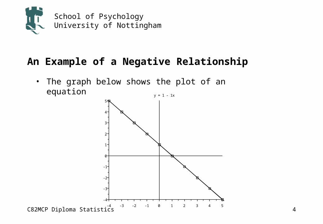
Example Data
• The data on the right is the mean number of words recalled by primary school children after listening to a spoken list of words
• Is there a linear relationship between these two variables
Age Mean Recalled5 5.75 66 5.86 6.17 6.27 6.88 78 7.39 79 7.7
C82MCP Diploma Statistics
School of PsychologyUniversity of Nottingham
8
Example Data
• When the data is plotted on a scattergraph the points do not all fit on a straight line
• We need to find a way to describe the best fitting straight line relationship.
44.55
5.56
6.57
7.58
8.59
4 5 6 7 8 9
Age
Mea
n R
ecal
led

C82MCP Diploma Statistics
School of PsychologyUniversity of Nottingham
9
Example Linear RegressionAge (X) Mean Recalled (Y) X squared Y squared XY
5 5.7 25 32.49 28.55 6 25 36 306 5.8 36 33.64 34.86 6.1 36 37.21 36.67 6.2 49 38.44 43.47 6.8 49 46.24 47.68 7 64 49 568 7.3 64 53.29 58.49 7 81 49 639 7.7 81 59.29 69.3
Sum 70 65.6 510 434.6 467.6Mean 7 6.56 51 43.46 46.76

C82MCP Diploma Statistics
School of PsychologyUniversity of Nottingham
10
Calculating the Slope
• The slope is given by:
• From the example calculations we get
• Therefore there is a positive relationship between age and the mean number of recalled words
b N XY X YN X2 ( X )2
b 10(467.6) (70)(65.6)
10(510) (70)2 0.42

C82MCP Diploma Statistics
School of PsychologyUniversity of Nottingham
11
Calculating the Intercept
• The intercept for the example data is given by:
• The intercept is
• For this data the regression line crosses the y axis at y=3.62
a Y bX
a 6.56 0.42(7) 3.62

C82MCP Diploma Statistics
School of PsychologyUniversity of Nottingham
12
Example Linear Equation
• For this example data the complete regression equation is given by
• If we look at one of the five year olds who scored a mean number of recalled words of 6 we find that the equation predicts that they should score 5.81
• The residual (i.e. the difference between the predicted score and the actual score) for this five year old is 0.19 which is small.
Predicted Mean Recalled(0.42)(Age)3.62

C82MCP Diploma Statistics
School of PsychologyUniversity of Nottingham
13
The Statistical Test of the Regression Equation
• "Does the regression equation significantly predict the data that have been obtained?"
• The way to approach this problem is on the basis of the variability in the Y scores that the regression equation accounts for.

C82MCP Diploma Statistics
School of PsychologyUniversity of Nottingham
14
Estimates of Variability
• The differences between the predicted and the observed scores are known as the residuals
• We can use the residuals as a measure of variability of the scores around the regression line

C82MCP Diploma Statistics
School of PsychologyUniversity of Nottingham
15
Testing the Regression Equation
• We can test the amount of variability that the regression equation accounts for using an F-ratio
• The estimate of variance used in the F-ratio is known as a Mean Square
• Mean Squares are defined as:
F Variance due to RegressionVariance due to Residuals
Mean Square =Sum of Squares
Degrees of Freedom
C82MCP Diploma Statistics
School of PsychologyUniversity of Nottingham
16
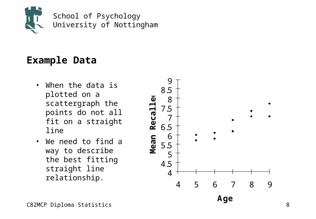
Sum of Square of the Regression
• The sum of squares of the regression can be calculated using the following formula
• where
SSRegression XY
X YN
2
SSX
SSX (X X )2 X2 ( X )2
N

C82MCP Diploma Statistics
School of PsychologyUniversity of Nottingham
17
Sum of Squares of the Residual
• The sum of squares of the residual can be calculated using the following formula
• where
SSResidual SSY SSRegression
SSY Y 2 ( Y )2
N

C82MCP Diploma Statistics
School of PsychologyUniversity of Nottingham
18
The Mean Squares
• The mean square for the regression is given by:
• The degrees of freedom for the residual are N-2, so the mean square for the residuals is:
MSRegression SSRegression
1
MSResidual SSResidual
N 2

C82MCP Diploma Statistics
School of PsychologyUniversity of Nottingham
19
Testing the Regression Equation
Age (X) Mean Recalled (Y) X squared Y squared XY5 5.7 25 32.49 28.55 6 25 36 306 5.8 36 33.64 34.86 6.1 36 37.21 36.67 6.2 49 38.44 43.47 6.8 49 46.24 47.68 7 64 49 568 7.3 64 53.29 58.49 7 81 49 639 7.7 81 59.29 69.3
Sum 70 65.6 510 434.6 467.6Mean 7 6.56 51 43.46 46.76
C82MCP Diploma Statistics
School of PsychologyUniversity of Nottingham
20
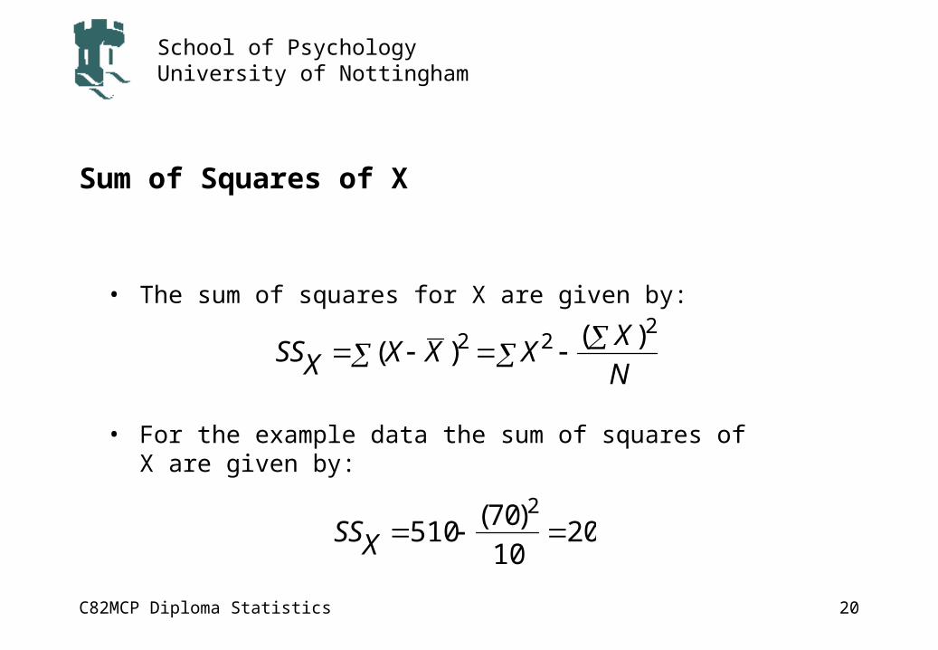
Sum of Squares of X
• The sum of squares for X are given by:
• For the example data the sum of squares of X are given by:
SSX 510 (70)2
1020
SSX (X X )2 X2 ( X )2
N
C82MCP Diploma Statistics
School of PsychologyUniversity of Nottingham
21
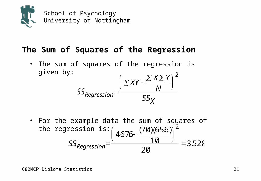
The Sum of Squares of the Regression
• The sum of squares of the regression is given by:
• For the example data the sum of squares of the regression is:
SSRegression XY
X YN
2
SSX
SSRegression 467.6 (70)(65.6)
10
2
203.528

C82MCP Diploma Statistics
School of PsychologyUniversity of Nottingham
22
The Sum of Squares of the Residual
• The sum of squares of the residual is given by:
• where
• For the example data the sum of squares of the residual is:
SSResidual SSY SSRegression
SSY Y 2 ( Y )2
N
SSResidual 434.6 (65.6)2
10 3.5280.736

C82MCP Diploma Statistics
School of PsychologyUniversity of Nottingham
23
The Mean Squares• The mean square for the regression is given by:
• The mean square for the residual is given by:
• The F-ratio is given by:
MSRegression SSRegression
13.528
MSResidual SSResidual
N 20.736
80.092
F MSRegressionMSResidual
3.5280.092
38.348
C82MCP Diploma Statistics
School of PsychologyUniversity of Nottingham
24
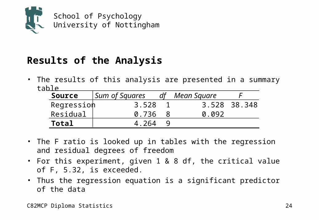
Results of the Analysis
• The results of this analysis are presented in a summary table
• The F ratio is looked up in tables with the regression and residual degrees of freedom
• For this experiment, given 1 & 8 df, the critical value of F, 5.32, is exceeded.
• Thus the regression equation is a significant predictor of the data
Source Sum of Squares df Mean Square FRegression 3.528 1 3.528 38.348Residual 0.736 8 0.092Total 4.264 9

C82MCP Diploma Statistics
School of PsychologyUniversity of Nottingham
25
Proportion of Variability accounted for
• One index of the success of the regression equation is the proportion of variability accounted for:
• This means the 83% of the variability in the dependent variable scores can be accounted for by the regression equation:
83.0264.4528.32
TotalSSRegressionSS
R
Predicted Mean Recalled(0.42)(Age)3.62

C82MCP Diploma Statistics
School of PsychologyUniversity of Nottingham
26
Summary
• The regression equation is a significant predictor of this data.
• There is a linear relationship between the mean number of words recalled and the age of the child
Predicted Mean Recalled(0.42)(Age)3.62