Embed Size (px)
Citation preview

C6 - Supply/Demand Market Model
Changes in Market Conditions using
Demand and Supply Concepts
Analysis - elasticities
Expanded Market Framework
Derived Demand and Supply
Marketing margin

Simple Market Model
Demand and Supply shifts
Quantitative analysis
Qualitative implications for equilibrium Price and QuantityInferences – Is S/D responsible for change in conditions?
using elasticities (own, cross, income)
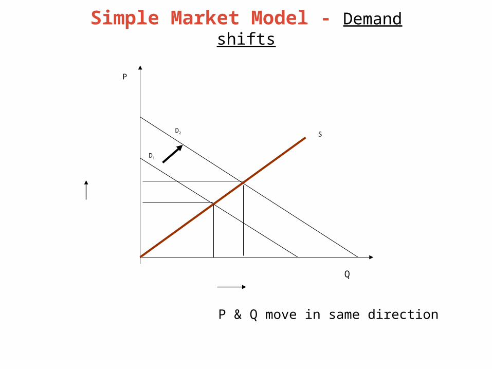
Simple Market Model - Demand shifts
P & Q move in same direction
D2
P
D1
S
Q

Simple Market Model - Supply shifts
P & Q move in opposite direction
D
P
S2
Q
S1

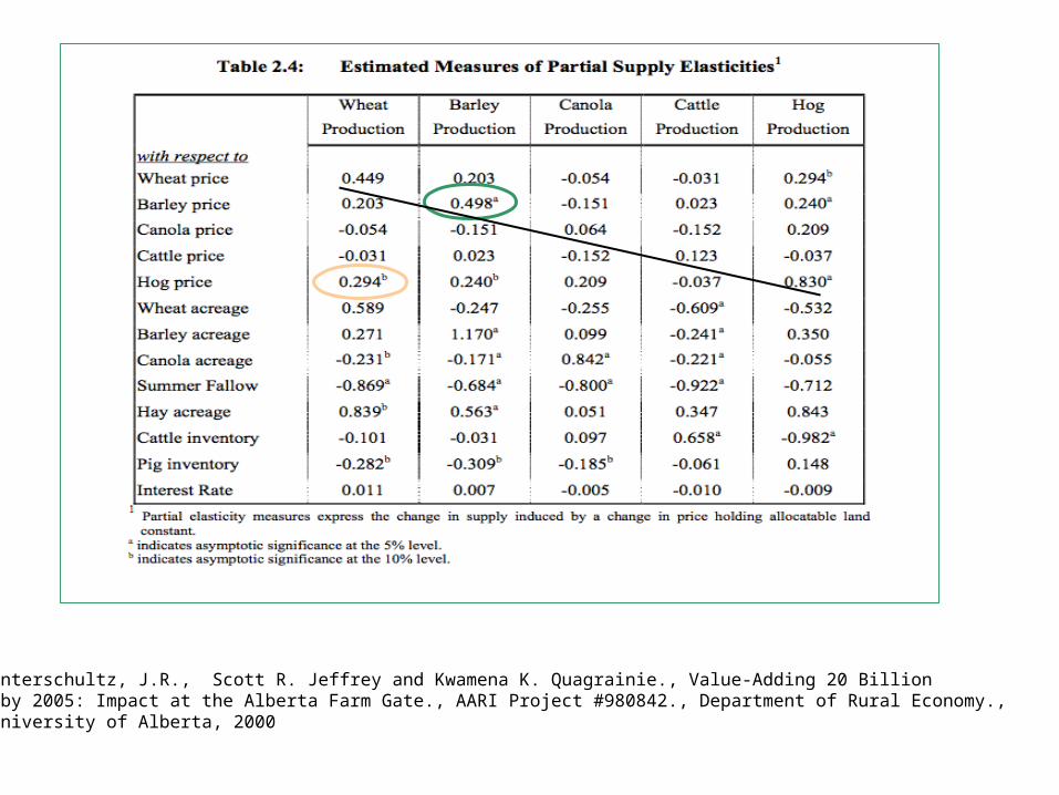
Unterschultz, J.R., Scott R. Jeffrey and Kwamena K. Quagrainie., Value-Adding 20 Billion by 2005: Impact at the Alberta Farm Gate., AARI Project #980842., Department of Rural Economy.,University of Alberta, 2000
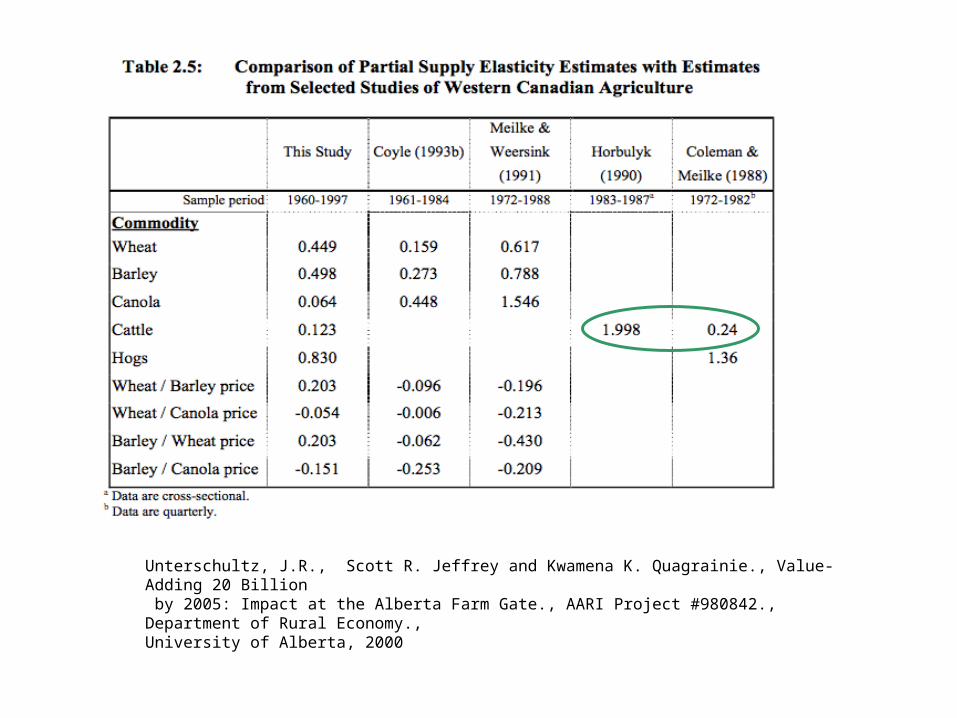
Unterschultz, J.R., Scott R. Jeffrey and Kwamena K. Quagrainie., Value-Adding 20 Billion by 2005: Impact at the Alberta Farm Gate., AARI Project #980842., Department of Rural Economy.,University of Alberta, 2000
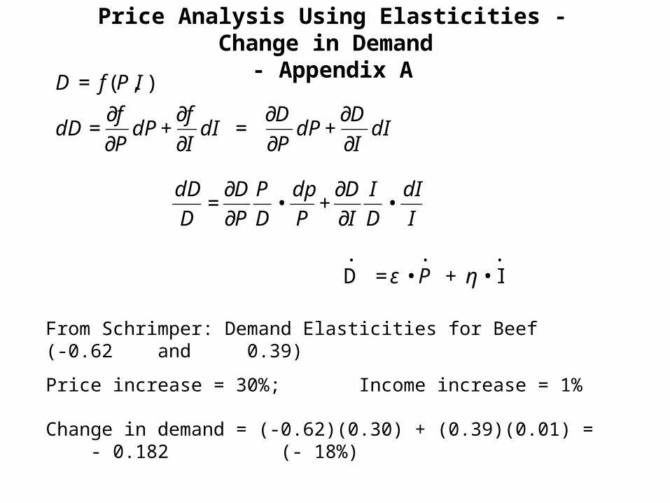
Price Analysis Using Elasticities - Change in Demand - Appendix A
€
D = f (P,I )
dD =∂f
∂PdP +
∂f
∂IdI =
∂D
∂PdP +
∂D
∂IdI
€
dD
D=∂D
∂P
P
D•dp
P+∂D
∂I
I
D•dI
I
From Schrimper: Demand Elasticities for Beef (-0.62 and 0.39)
Price increase = 30%; Income increase = 1%
Change in demand = (-0.62)(0.30) + (0.39)(0.01) = - 0.182 (- 18%)
€
D•
= ε • P•
+ η • I•
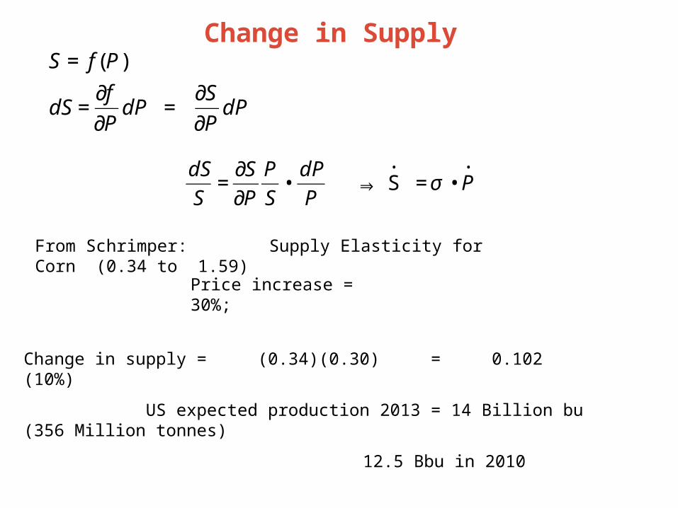
Change in Supply
€
S = f (P)
dS =∂f
∂PdP =
∂S
∂PdP
€
dS
S=∂S
∂P
P
S•dP
P ⇒ S
•
=σ • P•
From Schrimper: Supply Elasticity for Corn (0.34 to 1.59)
Price increase = 30%;
Change in supply = (0.34)(0.30) = 0.102 (10%)
US expected production 2013 = 14 Billion bu (356 Million tonnes)
12.5 Bbu in 2010
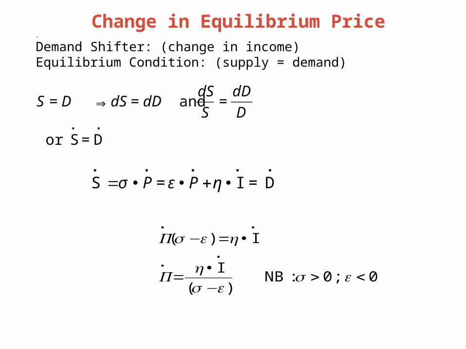
Change in Equilibrium Price.
Demand Shifter: (change in income)Equilibrium Condition: (supply = demand)
€
S = D ⇒ dS = dD and dS
S=dD
D
or S•
= D•
•••••
•+••= D = I = S ηεσ PP
0 ; 0 :NB )(
I
I)(
<>−•
=
•=−•
•
••
εσεσ
η
ηεσ
P
P
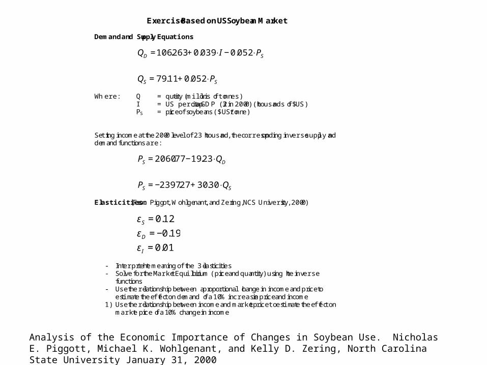
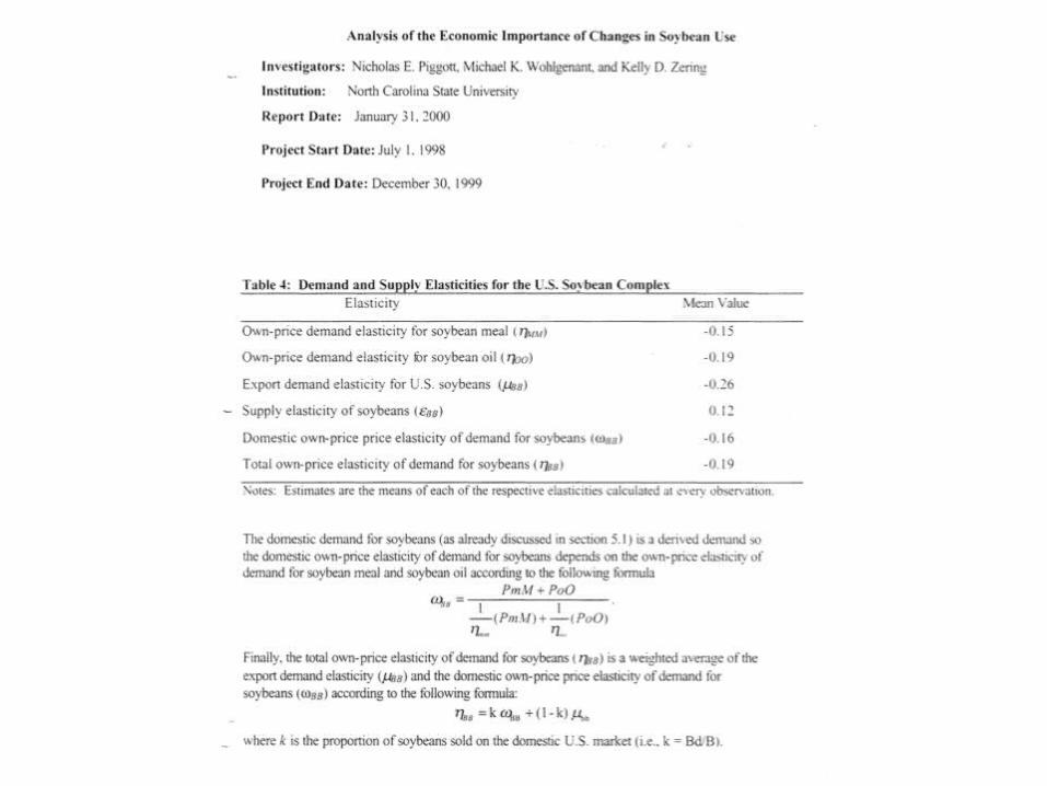
Exercise: Based on US Soybean Market Demand and Supply Equations
€
QD =106.263 + 0.039 ⋅ I − 0.052 ⋅PS
QS = 79.11+ 0.052 ⋅PS
Where: Q = quatity (millions of tonnes) I = US percapita GDP (23 in 2000) (thousands of $US) PS = price of soybeans ($US/tonne) Setting income at the 2000 level of 23 thousand, the corresponding inverse supply and demand functions are:
€
PS = 2060.77 −19.23⋅QD
PS = −2397.27 + 30.30 ⋅QS
Elasticities: (From Piggot, Wohlgenant, and Zering, NCS University, 2000)
€
εS = 0.12
εD = −0.19
ε I = 0.01
- Interpret the meaning of the 3 elasticities - Solve for the Market Equili brium (price and quantity) using the inverse
functions - Use the relationship between a proportional change in income and price to
estimate the eff ect on demand of a 10% increase in price and income 1) Use the relationship between income and market price to estimate the eff ect on
market price of a 10% change in income
Analysis of the Economic Importance of Changes in Soybean Use. Nicholas E. Piggott, Michael K. Wohlgenant, and Kelly D. Zering, North Carolina State University January 31, 2000
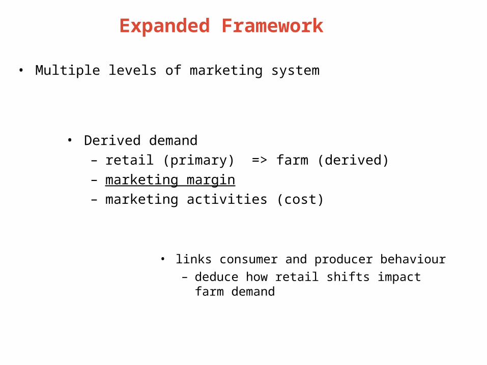
Expanded Framework
• Multiple levels of marketing system
• Derived demand
– retail (primary) => farm (derived)
– marketing margin
– marketing activities (cost)
• links consumer and producer behaviour
– deduce how retail shifts impact farm demand
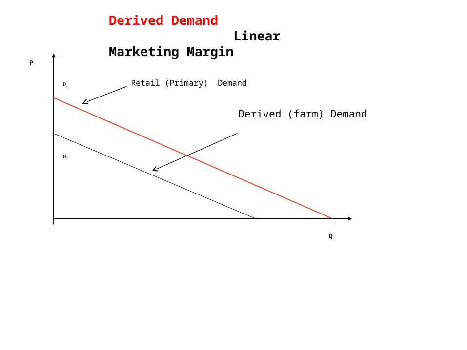
Derived (farm) Demand
Dr
P
Df
Q
Retail (Primary) Demand
Derived Demand Linear Marketing Margin

Assumptions: Linear Marketing Margin• Inputs: used in fixed proportions
– Retail Price = farm price + marketing inputs– constant returns - no economies of scale (marketing activities)
Implications
–fixed absolute margin
–Price elasticity - market levels
• Prices (marketing inputs)
– fixed/constant => perfectly elastic supply (competitive markets)
• Margin– temporal invariance

Elasticity and Derived Demand
Dr
P
Df
ε = 1
(P/Q)r
(P/Q)f
Demand elasticity at retail higher than farm level
ε =dQ
dP•P
Q and
P
Q
⎛
⎝ ⎜
⎞
⎠ ⎟r
> P
Q
⎛
⎝ ⎜
⎞
⎠ ⎟f ⎟⎟
⎠
⎞⎜⎜⎝
⎛•=
R
FRF P
Pεε
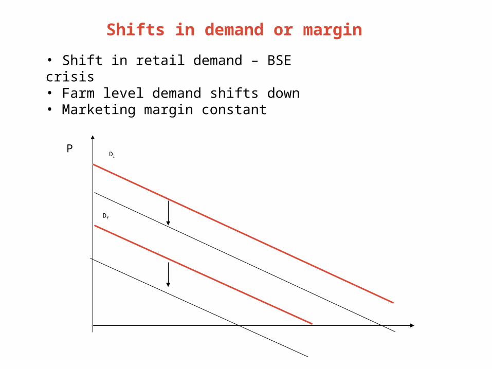
Shifts in demand or margin
• Shift in retail demand – BSE crisis• Farm level demand shifts down• Marketing margin constant
Dr
P
Df
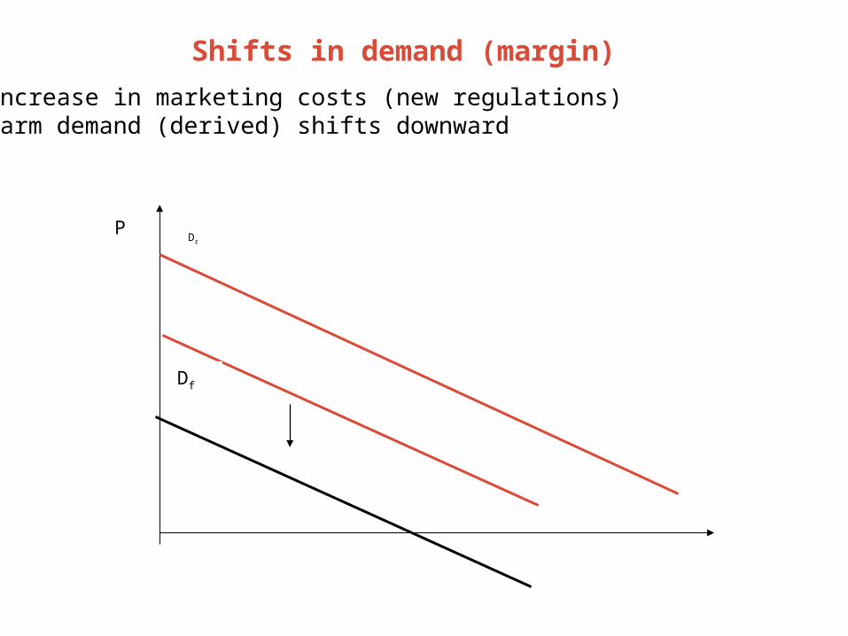
Shifts in demand (margin)
• Increase in marketing costs (new regulations)• Farm demand (derived) shifts downward
Dr
P
Df

Alternative Models
• Margin varies with quantity (proportional markup)• Decrease in marketing costs – as output expands
Demand elasticity at retail still higher than farm level
Dr
P
Q
Dfε=1

Derived Supply
Farm supply (primary)
Retail supply (derived)

Derived Supply and Demand
Quantity
DF
DR
PR
PSR
SF
Q*
PF
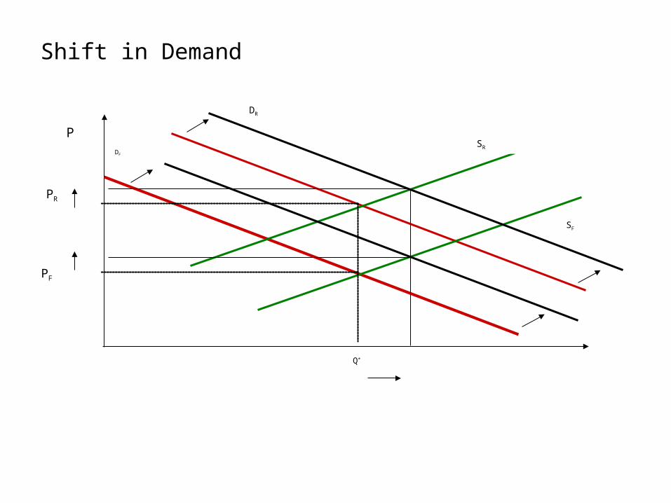
Shift in Demand
DF
DR
PR
PSR
SF
Q*
PF
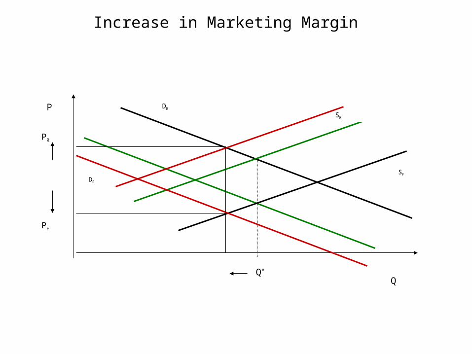
Increase in Marketing Margin
DF
DR
PR
PSR
SF
Q*
PF
Q
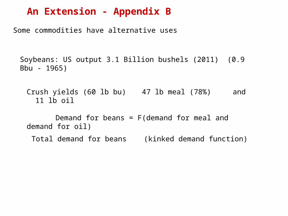
Some commodities have alternative uses
An Extension - Appendix B
Soybeans: US output 3.1 Billion bushels (2011) (0.9 Bbu - 1965)
Crush yields (60 lb bu) 47 lb meal (78%) and 11 lb oil
Demand for beans = F(demand for meal and demand for oil)
Total demand for beans (kinked demand function)

CBOT Soybean Price (2003 – 2011)
$ 13
$ 6
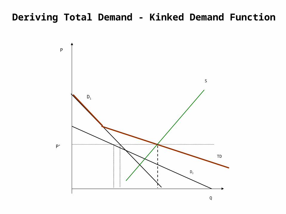
S
D1
D2
TD
P*
P
Q
Deriving Total Demand - Kinked Demand Function