Embed Size (px)
Citation preview

No d’ordre : ANNEE 2017
HABILITATION A DIRIGER DES RECHERCHES
UNIVERSITE DE RENNES 1sous le sceau de l’Universite Europeenne de Bretagne
Mention InformatiqueEcole doctorale Matisse
presentee par
Cedric Tedeschi
preparee a l’unite de recherche IRISA (UMR 6074)Composante universitaire: ISTIC
Distributed
Chemically-Inspired
Runtimes for
Large Scale Adaptive
Computing Platforms
HDR soutenue le 11 avril 2017 a Rennesdevant le jury compose de :
Claudia Di NapoliChargee de recherche / CNR / Rapporteuse
Jean-Louis GiavittoDirecteur de recherche / CNRS / Rapporteur
Jean-Marc JezequelProfesseur / U. de Rennes 1 / President
Johan MontagnatDirecteur de recherche / CNRS / Examinateur
Christine MorinDirectrice de recherche / Inria / Examinatrice
Thierry PriolDirecteur de recherche / Inria / Examinateur
Pierre SensProfesseur / U. Pierre et Marie Curie / Rapporteur

2

A Abiga[e]l, telle qu’en elle-meme.
3

4

Take me by the hand nowIt’s been a long, long time since I’ve stepped outsideTo the morning sun
— Babyshambles
5

6

Contents
Introduction 9
1 The Chemical Programming Style 171.1 Chemically-inspired programming . . . . . . . . . . . . . . . . . . . . . . . . . . . . . . . . . 171.2 HOCL . . . . . . . . . . . . . . . . . . . . . . . . . . . . . . . . . . . . . . . . . . . . . . . . . 181.3 Close models . . . . . . . . . . . . . . . . . . . . . . . . . . . . . . . . . . . . . . . . . . . . . 19
2 On the Runtime Complexity of Concurrent Multiset Rewriting 212.1 The complexity problem . . . . . . . . . . . . . . . . . . . . . . . . . . . . . . . . . . . . . . . 212.2 Model . . . . . . . . . . . . . . . . . . . . . . . . . . . . . . . . . . . . . . . . . . . . . . . . . 22
2.2.1 Modeling of the rule’s condition . . . . . . . . . . . . . . . . . . . . . . . . . . . . . . . 222.2.2 Structuring of the multiset . . . . . . . . . . . . . . . . . . . . . . . . . . . . . . . . . 232.2.3 NP-hardness and the subgraph isomorphism problem . . . . . . . . . . . . . . . . . . . 24
2.3 Calibre and the PMJA Algorithm . . . . . . . . . . . . . . . . . . . . . . . . . . . . . . . . . . 252.3.1 Calibre of a rule . . . . . . . . . . . . . . . . . . . . . . . . . . . . . . . . . . . . . . . 252.3.2 The PMJA algorithm . . . . . . . . . . . . . . . . . . . . . . . . . . . . . . . . . . . . 27
2.4 Discussion . . . . . . . . . . . . . . . . . . . . . . . . . . . . . . . . . . . . . . . . . . . . . . 302.4.1 Summary . . . . . . . . . . . . . . . . . . . . . . . . . . . . . . . . . . . . . . . . . . . 302.4.2 Approximation and distribution . . . . . . . . . . . . . . . . . . . . . . . . . . . . . . . 30
3 Adaptive Atomic Capture of Multiple Molecules 333.1 The importance of being atomic . . . . . . . . . . . . . . . . . . . . . . . . . . . . . . . . . . . 333.2 System model . . . . . . . . . . . . . . . . . . . . . . . . . . . . . . . . . . . . . . . . . . . . . 35
3.2.1 Data and Rules Dissemination . . . . . . . . . . . . . . . . . . . . . . . . . . . . . . . 353.2.2 Discovery Protocol . . . . . . . . . . . . . . . . . . . . . . . . . . . . . . . . . . . . . . 353.2.3 Fault tolerance . . . . . . . . . . . . . . . . . . . . . . . . . . . . . . . . . . . . . . . . 36
3.3 Protocol . . . . . . . . . . . . . . . . . . . . . . . . . . . . . . . . . . . . . . . . . . . . . . . . 363.3.1 Pessimistic sub-protocol . . . . . . . . . . . . . . . . . . . . . . . . . . . . . . . . . . . 363.3.2 Optimistic sub-protocol . . . . . . . . . . . . . . . . . . . . . . . . . . . . . . . . . . . 373.3.3 Sub-protocol mixing . . . . . . . . . . . . . . . . . . . . . . . . . . . . . . . . . . . . . 393.3.4 Dormant nodes . . . . . . . . . . . . . . . . . . . . . . . . . . . . . . . . . . . . . . . . 403.3.5 Multiple-rules programs . . . . . . . . . . . . . . . . . . . . . . . . . . . . . . . . . . . 403.3.6 Protocol’s safety and liveness . . . . . . . . . . . . . . . . . . . . . . . . . . . . . . . . 41
3.4 Evaluation . . . . . . . . . . . . . . . . . . . . . . . . . . . . . . . . . . . . . . . . . . . . . . . 423.4.1 Single-rule experiments . . . . . . . . . . . . . . . . . . . . . . . . . . . . . . . . . . . 433.4.2 Multiple-rules experiments . . . . . . . . . . . . . . . . . . . . . . . . . . . . . . . . . 46
3.5 Conclusion . . . . . . . . . . . . . . . . . . . . . . . . . . . . . . . . . . . . . . . . . . . . . . 47
4 Implementing Distributed Chemical Machines 494.1 The need for chemical run-time environments . . . . . . . . . . . . . . . . . . . . . . . . . . . 49
4.1.1 Physical parallelism . . . . . . . . . . . . . . . . . . . . . . . . . . . . . . . . . . . . . 50
7

4.1.2 Physical distribution . . . . . . . . . . . . . . . . . . . . . . . . . . . . . . . . . . . . . 504.2 A hierarchical reactor . . . . . . . . . . . . . . . . . . . . . . . . . . . . . . . . . . . . . . . . 50
4.2.1 Overview . . . . . . . . . . . . . . . . . . . . . . . . . . . . . . . . . . . . . . . . . . . 514.2.2 Efficient condition checking and inertia detection . . . . . . . . . . . . . . . . . . . . . 514.2.3 Tree reorganisation . . . . . . . . . . . . . . . . . . . . . . . . . . . . . . . . . . . . . . 534.2.4 Prototype . . . . . . . . . . . . . . . . . . . . . . . . . . . . . . . . . . . . . . . . . . . 544.2.5 Experimental evaluation . . . . . . . . . . . . . . . . . . . . . . . . . . . . . . . . . . . 55
4.3 A fully-decentralised higher-order reactor . . . . . . . . . . . . . . . . . . . . . . . . . . . . . 574.3.1 General execution scheme . . . . . . . . . . . . . . . . . . . . . . . . . . . . . . . . . . 584.3.2 Molecule searching and inertia detection . . . . . . . . . . . . . . . . . . . . . . . . . . 594.3.3 Higher-order . . . . . . . . . . . . . . . . . . . . . . . . . . . . . . . . . . . . . . . . . 604.3.4 Prototype . . . . . . . . . . . . . . . . . . . . . . . . . . . . . . . . . . . . . . . . . . . 624.3.5 Experimental evaluation . . . . . . . . . . . . . . . . . . . . . . . . . . . . . . . . . . . 63
4.4 Conclusion . . . . . . . . . . . . . . . . . . . . . . . . . . . . . . . . . . . . . . . . . . . . . . 65
5 Decentralising Workflow Execution 675.1 Workflows, workflow managers, and decentralisation . . . . . . . . . . . . . . . . . . . . . . . 675.2 Shared-space based coordination . . . . . . . . . . . . . . . . . . . . . . . . . . . . . . . . . . 685.3 Chemical workflow specification . . . . . . . . . . . . . . . . . . . . . . . . . . . . . . . . . . . 695.4 GinFlow . . . . . . . . . . . . . . . . . . . . . . . . . . . . . . . . . . . . . . . . . . . . . . . . 71
5.4.1 The HOCL distributed engine . . . . . . . . . . . . . . . . . . . . . . . . . . . . . . . 725.4.2 Resilience . . . . . . . . . . . . . . . . . . . . . . . . . . . . . . . . . . . . . . . . . . . 735.4.3 The executors . . . . . . . . . . . . . . . . . . . . . . . . . . . . . . . . . . . . . . . . 735.4.4 Client interfaces . . . . . . . . . . . . . . . . . . . . . . . . . . . . . . . . . . . . . . . 74
5.5 Experimental validation . . . . . . . . . . . . . . . . . . . . . . . . . . . . . . . . . . . . . . . 745.5.1 Performance . . . . . . . . . . . . . . . . . . . . . . . . . . . . . . . . . . . . . . . . . 765.5.2 Impact of the executor and messaging middleware . . . . . . . . . . . . . . . . . . . . 765.5.3 Resilience . . . . . . . . . . . . . . . . . . . . . . . . . . . . . . . . . . . . . . . . . . . 77
5.6 Decentralising workflow execution in literature . . . . . . . . . . . . . . . . . . . . . . . . . . 775.7 Conclusion . . . . . . . . . . . . . . . . . . . . . . . . . . . . . . . . . . . . . . . . . . . . . . 78
6 Injecting Adaptiveness in (Decentralised) Workflow Execution 816.1 The need for dynamically adapting workflows . . . . . . . . . . . . . . . . . . . . . . . . . . . 81
6.1.1 Cold adaptation . . . . . . . . . . . . . . . . . . . . . . . . . . . . . . . . . . . . . . . 816.1.2 Hot adaptation . . . . . . . . . . . . . . . . . . . . . . . . . . . . . . . . . . . . . . . . 82
6.2 HOCL-based adaptive workflows . . . . . . . . . . . . . . . . . . . . . . . . . . . . . . . . . . 836.2.1 HOCL abstract adaptive workflow . . . . . . . . . . . . . . . . . . . . . . . . . . . . . 836.2.2 Adaptation rules . . . . . . . . . . . . . . . . . . . . . . . . . . . . . . . . . . . . . . . 846.2.3 Execution . . . . . . . . . . . . . . . . . . . . . . . . . . . . . . . . . . . . . . . . . . . 846.2.4 Generalising . . . . . . . . . . . . . . . . . . . . . . . . . . . . . . . . . . . . . . . . . . 85
6.3 Adaptiveness in GinFlow . . . . . . . . . . . . . . . . . . . . . . . . . . . . . . . . . . . . . . 866.3.1 Implementation . . . . . . . . . . . . . . . . . . . . . . . . . . . . . . . . . . . . . . . . 866.3.2 Client interfaces . . . . . . . . . . . . . . . . . . . . . . . . . . . . . . . . . . . . . . . 86
6.4 Experimental evaluation . . . . . . . . . . . . . . . . . . . . . . . . . . . . . . . . . . . . . . . 876.5 Adapting the workflow shape in literature . . . . . . . . . . . . . . . . . . . . . . . . . . . . . 886.6 Conclusion . . . . . . . . . . . . . . . . . . . . . . . . . . . . . . . . . . . . . . . . . . . . . . 89
Conclusion 91
Bibliography 95
8

Introduction
The quest for distributed programming styles
Every time a new type of computing platforms appears, the challenge comes back: increasing the amount ofcomputing resources does not guarantee that such a computing power will be adequately exploited. There isa crucial need to offer programming tools, styles, abstractions that will allow the user to easily specify andefficiently run programs over the platform.
The difficulty stands in the self-contradiction conveyed by such a venture: ease most of the time meansraise the level of abstraction, while being efficient requires sometimes to have a manual control over thedetails of the platform’s architecture. The quest for the right level of abstraction can be traced back to thefoundational crisis traversed by mathematicians in the early twentieth century, and which saw the rise ofthe field of computability, which was trying to formally decide what can be computed and what cannot. Atthat time, the question of the programming style was not the primary concern.
In his 1936 seminal paper about computability [100], Alan Turing describes first his abstract machines inthe most basic way possible, to avoid any misunderstanding. In particular, a machine includes a very limitedinstruction set : move to the next symbol left or right, read one symbol on the tape, change its inner state.Yet, at some point, and for the sake of describing his machines in a more concise way, Turing introduceswhat he refers to as an abbreviation: the skeleton tables, which allows to describe more easily machines, withgeneric functionalities that can take parameters. The key point is that, as he states [100]:
The skeleton tables are to be regarded as nothing but abbreviations: they are not essential. Solong as the reader understands how to obtain the complete tables from the skeleton tables, thereis no need to give any exact definitions in this connection.
While Turing presents the skeleton tables as not essential (in the sense that it will not change anythingin terms of computability), it is still a small step towards raising the level of abstraction, towards moreexpressiveness.
A few years later, two main families of programming languages emerged. One was based on what is nowreferred to as the Von Neumann architecture model of a computer [102], which, while simple, offered a modelencompassing most computer architectures in those days of rapidly changing technology. The Von Neumannmodel paved the way for the family of imperative languages. The second family of programming style tookits roots in Lambda-calculus, developed by Alonzo Church in an attempt at building a formal ground tocomputability and generally considered equivalent to other mathematical model of computability such aspartial recursive functions [34]. While less correlated to the physical architecture of a digital computer,lambda-calculus was the ground the other family of programming languages, called functional programming.
To put it simply, while imperative programming requires the programmer to deal with explicit machineryinstructions such as reading and writing memory cells and incrementing pointers, functional programmingfocus on building a functional solution to a problem, i.e., a solution involving merely the evaluation of acomposition of functions. While the passionate debate about the pros and cons of these two styles is not theprimary concern of the present dissertation, the point is that the functional style abstracts out the detailsof the underlying architecture. This is not true in the case of imperative programming which explicitlydeal with memory manipulation, even if some imperative languages, such as C, offers an increased level ofabstractions when compared with assembly languages.
9

More generally, functional programming is to be considered as a declarative paradigm. Declarativeprogramming [68] tries to separates the logic of a computation (“what we want to do”) from its control (“howto achieve it”). More precisely, in such an approach, while the “what” is to be defined by the programmer,the “how” is ideally left to the runtime system, the engine of the execution environment. Unfortunately,increasing the level of abstraction comes at a price: the more declarative (or expressive) a language is, themore difficult it becomes to have it executed, in average, in an efficient way.
This picture can be extended to distributed computing. Even if of a higher-level of abstraction, messagepassing can be thought of as the assembly language of distributed systems: one computer sending bits toanother one through a channel. Message passing does not constitute a programming model in itself, in thesense that it was not developed to ease the programmer’s specification work. Remote Procedure Call (RPC)is a programming model allowing to call procedures to be run on distant computing facilities from within alocal program. It operates in a client-server fashion: the client, which is running a program locally, relies onsome remote procedure for parts of its execution. When this remote procedure needs to be called, the clientsends the parameters on which to apply the function. The server receives them, runs the function on them,and sends the result of the execution back to the client, that can now use it for subsequent local computationsteps. RPC was also developed as an extension of the object-oriented model, as proposed by RMI [42] in theJava world or by CORBA [92]. The principles of RMI and CORBA are similar to those of RPC except thatfunctions called are methods from objects, these objects being hosted by distinct computers, or at least bydistinct Java virtual machines in the case of RMI.
CORBA and similar mechanisms were used in the development of Grid computing, in which the com-puting power of heterogeneous geographically distributed computing facilities (clusters or desktops) is ag-gregated into a single entity: the grid. Taking into account the extra requirements related to the scale, theheterogeneity and the unreliable nature of large scale platforms, led to the rise of the component model [98].
Concretely speaking, the component model [98] and its different flavours and implementations [15, 24, 14]were developed to answer to the need to compose existing pieces of stand-alone software. As for the Object-Oriented programming style, reuse and ease of composition were the main drivers behind the development ofthe component model. However, new needs were also to be tackled, mainly heterogeneity and distribution:the software services to be composed can rely on different languages and run on different computing facilities.Yet, we need a way to encapsulate them so as to make them communicate transparently. A common case forcomponents is code coupling, as explained in the paper by Denis et. al [37]: the authors describe a simplecode coupling-based application that simulates the transport of chemical products in a porous medium inthe context of a chemical 3D simulation. In this example, two codes have been developed separately bydifferent teams in different languages: a first code computes the chemical product’s density and a second onesimulates the medium’s porosity. These two codes typically run on different distant computing facilities. Torun the whole simulation, an appealing solution would be to combine these two codes (instead of trying tobuild another code from scratch. Still, we have to solve the heterogeneity and communication issues. In ourexample, two components are to be deployed. Each service will be encapsulated into a component able tocommunicate with the other, following the use and provide paradigm, each component having a set of portsof two possible kinds: ports providing data to others, called facets, and ports receiving data from others,called receptacles.
The Internet of Services
The last shift the world witnessed in terms of digital ecosystem led to the rise of a global platform deliveringa virtually unlimited computing power including on one side very large centralised infrastructures, resultingfrom the morphing of computing clusters into utility computing centers (or clouds), and on the other side amyriad of less heavy devices such as smartphones, tablets and TVs. This global digital ecosystem revolvesaround the Internet backbone and supports a boundless number of computing services ranging from allpossible brands of on-line business services to scientific data storing and processing services helping scientistswith their researches.
In the context of the Internet of Services, the term service encompasses a large set of functionalities,implemented by various languages, supported by heterogeneous software stacks and systems running on
10
different hardware. Still, they tend to have a set of common characteristics. Let us try to define what aservice is. I think we can safely state three basic characteristics a service must have: i) an unambiguousself-contained functionality, ii) a network-enabled, well-defined API, iii) the ability to be composed withother services.
The last point raises a lot of questions related to the programming abstractions, concepts, architecturesand tools that could enact a service composition in such an environment. Interconnecting computing serviceshas been a major topic in both industrial and academic environments since the rise of the dot-com era in themiddle of the 1990s. Component architectures and workflows have appeared to be the two major paradigmsto handle this problem.
Components vs workflows
The limitation of the component models stands primarily in that these ports mentioned above are specificto an application and can only be statically defined. In other words, a component is compatible only with apredefined set of other components which have been constrained with a symmetric set of ports, in order tobuild the targeted application. At run time, the components cooperate in a remote procedure call fashion.This can be seen as spatial composition: services are all present at the same time, and these service boxesare interconnected in the application plane, so that they can call each others. Spatial composition relieson the encapsulation of the services to be composed: the details of the bindings between components aredeveloped inside the components, through stubs and skeletons acting as proxies to the other components.Unfortunately, this static encapsulation hinders the possibility for one service to communicate with servicesother than those predefined for this specific application’s purpose.
The other kind of composition, still as described in [22], is temporal composition. By temporal, it is meantthat this kind of composition expresses the actual control flow between the set of services involved: it focuson when services need each others, in other words, what are the data and control dependencies betweenthem. This paradigm is also known as distributed workflow computing. A workflow is most of the time adirected acyclic graph where each vertex is a task and each edge is a dependency between two tasks, eithera control dependency or a data dependency.
In workflow computing, composed services are not really encapsulated: the composition of the servicesitself is described in a distinct file, to be read and enacted by a workflow engine, or service orchestrator,which is external to the services. The services do not know themselves how to take part in the executionand its coordination (i.e., the mechanisms enforcing the satisfaction of the dependencies expressed in theworkflow). Basically, a service does nothing except waiting for a call. This is where the orchestrator isbrought into the picture. The orchestrator enacts the workflow described in the description file. At runtime, it takes care of the coordination by triggering the tasks in the order specified. It acts as a centralcoordinator. Every notification of the completion of a service, or even intermediate data produced will gothrough it.
We generally distinguish two kinds of workflow: abstract ones and concrete ones. An abstract workflowis typically a DAG of tasks where tasks represent what is to be done. This is the functional specificationof the workflow. A fully abstract workflow does not include any technical information such as how to enactthese tasks or what specific executable file will actually get called to realise each task. On the other side ofthe spectrum, a concrete workflow contains all the technical details needed to actually execute the workflowand answers questions such as where are the data?, where is the executable file to be used?, what computingnodes will host the execution of what task?
This discussion leads us to Table 0.1 which summarizes the differences between component-based appli-cations and workflows. The first dimension, the type of composition, is the essence of each paradigm. It hasbeen discussed above and in some way subsumes the two following dimensions: binding and coupling.
The second dimension in Table 0.1, binding, refers to when the communication between two servicestaking part in the workflow is actually established. In workflows, it can be done just-in-time. It is useless tobind any service to perform some task before its incoming dependencies are satisfied. Late binding bringsflexibility to the execution as it allows to choose the best service available on the platform when the enactment
11
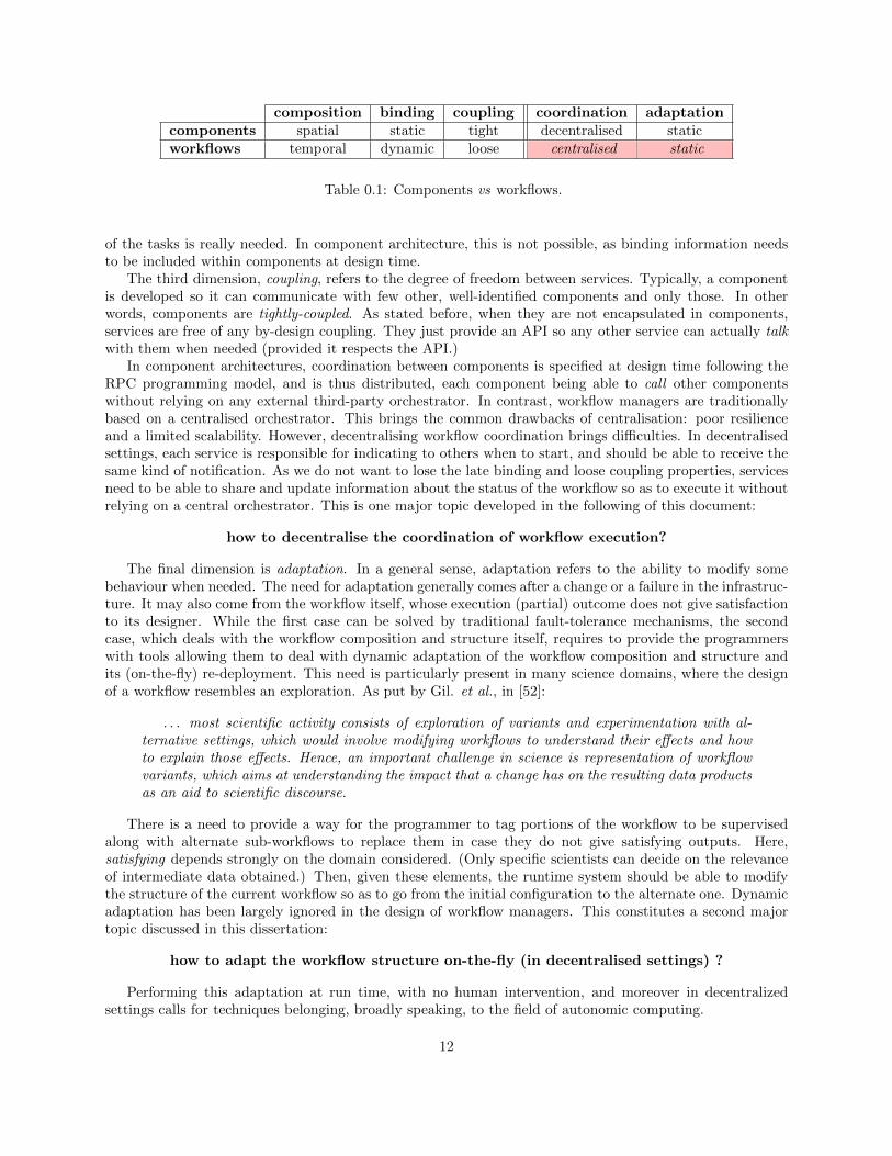
composition binding coupling coordination adaptationcomponents spatial static tight decentralised staticworkflows temporal dynamic loose centralised static
Table 0.1: Components vs workflows.
of the tasks is really needed. In component architecture, this is not possible, as binding information needsto be included within components at design time.
The third dimension, coupling, refers to the degree of freedom between services. Typically, a componentis developed so it can communicate with few other, well-identified components and only those. In otherwords, components are tightly-coupled. As stated before, when they are not encapsulated in components,services are free of any by-design coupling. They just provide an API so any other service can actually talkwith them when needed (provided it respects the API.)
In component architectures, coordination between components is specified at design time following theRPC programming model, and is thus distributed, each component being able to call other componentswithout relying on any external third-party orchestrator. In contrast, workflow managers are traditionallybased on a centralised orchestrator. This brings the common drawbacks of centralisation: poor resilienceand a limited scalability. However, decentralising workflow coordination brings difficulties. In decentralisedsettings, each service is responsible for indicating to others when to start, and should be able to receive thesame kind of notification. As we do not want to lose the late binding and loose coupling properties, servicesneed to be able to share and update information about the status of the workflow so as to execute it withoutrelying on a central orchestrator. This is one major topic developed in the following of this document:
how to decentralise the coordination of workflow execution?
The final dimension is adaptation. In a general sense, adaptation refers to the ability to modify somebehaviour when needed. The need for adaptation generally comes after a change or a failure in the infrastruc-ture. It may also come from the workflow itself, whose execution (partial) outcome does not give satisfactionto its designer. While the first case can be solved by traditional fault-tolerance mechanisms, the secondcase, which deals with the workflow composition and structure itself, requires to provide the programmerswith tools allowing them to deal with dynamic adaptation of the workflow composition and structure andits (on-the-fly) re-deployment. This need is particularly present in many science domains, where the designof a workflow resembles an exploration. As put by Gil. et al., in [52]:
. . . most scientific activity consists of exploration of variants and experimentation with al-ternative settings, which would involve modifying workflows to understand their effects and howto explain those effects. Hence, an important challenge in science is representation of workflowvariants, which aims at understanding the impact that a change has on the resulting data productsas an aid to scientific discourse.
There is a need to provide a way for the programmer to tag portions of the workflow to be supervisedalong with alternate sub-workflows to replace them in case they do not give satisfying outputs. Here,satisfying depends strongly on the domain considered. (Only specific scientists can decide on the relevanceof intermediate data obtained.) Then, given these elements, the runtime system should be able to modifythe structure of the current workflow so as to go from the initial configuration to the alternate one. Dynamicadaptation has been largely ignored in the design of workflow managers. This constitutes a second majortopic discussed in this dissertation:
how to adapt the workflow structure on-the-fly (in decentralised settings) ?
Performing this adaptation at run time, with no human intervention, and moreover in decentralizedsettings calls for techniques belonging, broadly speaking, to the field of autonomic computing.
12

Autonomic Computing
As stated before, as systems get more complicated, alternate programming models need to be proposed. Moreprecisely, above a certain level of complexity, a top-down approach for specification may appear necessary:the system’s specification is refined step by step starting from a high level view of how the system is supposedto behave. In other words, it supposes having several levels of specifications for the same system, as thewhole system cannot be specified in detail at once using a unique language. Also, facing such a complexitymeans that human intervention at run time is not desirable and simply not feasible. Systems must be ableto manage themselves, they need to become autonomic. As written in IBM’s whitepaper on autonomiccomputing [57]:
Autonomic Computing helps to address complexity by using technology to manage technology.The term autonomic is derived from human biology. The autonomic nervous system monitorsyour heartbeat, checks your blood sugar level and keeps your body temperature close to 98.6 ◦Fwithout any conscious effort on your part. In much the same way, self-managing autonomiccapabilities anticipate IT system requirements and resolve problems with minimal human inter-vention.
When autonomic computing gained momentum in the early 2000s, it echoed the pioneering works incybernetics conducted fifty years earlier. In the 1950s, nature was already a source of inspiration, and inparticular the human brain, as developed by William Ross Ashby in his book Design for a Brain [6]. Theanalogy between a digital autonomic system and the autonomous nervous system was exposed through anexample of homeostasis, namely glucose regulation:
. . . if the concentration should fall below about 0.06 percent, the tissues will be starved of theirchief source of energy; if the concentration should rise above about 0.18 percent, other undesirableeffects will occur. If the blood-glucose concentration falls below about 0.07 percent, the adrenalglands secrete adrenaline, which causes the liver to turn its stores of glycogen into glucose. Thispasses into the blood and the blood glucose concentration drop is opposed. Further, a fallingblood-glucose also removed by muscles and skin, and if the blood-glucose concentration exceeds0.18 percent, the kidneys excrete excess glucose . . .
Let us linger a bit on this description: It mixes two questions: what are the threshold values to startregulating? and how the regulation is achieved? Actually, it seems that the what to do could be simplifiedby the two following rules (let c the blood glucose concentration):{
c < 0.07%→ secrete adrenalin
c > 0.15%→ secrete insulin
These two simple lines may constitute the high-level rules the brain needs to adhere to in order to maintainglucose blood concentration in survival areas: it is the specification. To actually achieve the constraintsexpressed by the rules, it relies on complex chemistry taking place within the body: it is the implementation.Autonomic systems advocate the separation of concerns between specification and implementation, whichshould not be addressed at once. As stated by Parashar and Hariri in [80] in 2004:
Conceptual research issues and challenges include defining appropriate abstractions and mod-els for specifying, understanding, controlling, and implementing autonomic behaviors.
The need for adequate programming models, in particular for specification purposes, has been raisedonce again with the rise of autonomic computing.
13

Chemically-inspired Programming
So what? What programming style should be used to bring decentralization and adaptiveness to large scale(workflow) coordination? The old debate between imperative and declarative programming is still highlyrelevant when it comes to separate specification from implementation in large distributed systems. In a 2010paper devising a rule-based language to specify distributed applications such as communication protocols,Grumbach and Wang wrote [54]:
Rule-based languages allow to obtain code about two orders of magnitude more concise thanstandard imperative programming languages.
Rule-based languages are a typical example of a declarative language where the what is explicitly statedthrough a set of rules to be satisfied. This is why it has been extensively used in expert systems [55]. Whilerule-based programming styles are appealing in our case, we still need one which can easily capture thedistributed nature of the coordination while offering ways to express dynamic adaptation. This is where theprogramming style brought about by artificial chemistries comes into the picture [39].
The chemically-inspired programming style was initially proposed with the objective of offering a declar-ative programming style for highly parallel programs. In a 1988 paper [9], the authors propose a chemically-inspired programming style based on multiset rewriting. They establish the absence of structure in data andof sequentiality in control as the norm. And because no data structuring and plain parallelism is the rule,they can become implicit. In the end, the programming style proposed can be summarized as a set of rulesto be applied concurrently on some input unstructured data, more formally a multiset.
At design time, the programmer just needs to define the set of rules to be applied on the multiset,and specifies the initial content of the multiset (in more traditional terms, input data). The programmerassumes that, at run time, these rules are to be applied in no specific order on the multiset. There is onlyone assumption: if one rule can be applied given the state of the data, one rule will be applied in a finitetime. It is the duty of the runtime implementor to make the relevant choices to implement this relativefreedom efficiently.
The higher order in chemical programming was introduced in 2007 [11], through the proposal of theHigher-Order Chemical Language (HOCL). In HOCL, rules can be applied to other rules. In other words,rules can appear or disappear from the program depending on the state of the multiset. This paves the wayfor dynamic adaptation when using a rule-based programming style.
Chemical computing at the rescue; At the rescue of chemical computing
This dissertation presents a series a works conducted between 2009 and 2016 pursuing the idea that higher-order chemical programming is a relevant programming style for the autonomous execution of applicationsat large scale. Still, until recently, a significant barrier towards the actual adoption of the chemical stylestood in the lack of runtime systems supporting it, especially at large scale. This is another major topicdeveloped in this dissertation:
what are the concepts, algorithmics and software pilots needed towards a largely distributedruntime system supporting the chemical programming style ?
Outline
The first part of this dissertation presents the results obtained on this specific research tracks. Chapter 1presents the chemical programming model in more detail. Chapter 2 discusses its complexity at run time.Chapter 3 goes large scale and addresses the algorithmic challenges raised by distributing the runtime ofchemical programs. Chapter 4 presents the design, implementation and experimental validation of actualdistributed chemical machines.
14

The second part of this dissertation builds upon the idea that the chemical model, as a representativeof concurrent rule-based programming eases the design of decentralised and adaptive coordination modelsand environments for workflow execution. Chapter 5 describes the design, implementation and experimentalvalidation of GinFlow, a decentralised workflow executor whose execution agents rely on a chemical engine attheir core. Chapter 6 shows how such a decentralised workflow execution can be enhanced with adaptivenessat the workflow level to provide workflow developers with a flexible design tool where different workflowalternatives can be designed and enacted dynamically.
15

Chapter 1
The Chemical Programming Style
In this chapter, we discuss the chemical programming style and present the Higher-Order Chemical Language(HOCL), the language chosen to underlie our work on workflow execution and adaptation and prototype theGinFlow software, as presented later in Chapters 5 and 6. We finally mention few close models from theliterature.
1.1 Chemically-inspired programming
Chemical programming was born from the idea that trying to bring sequential programming models to theparallel world is not just a matter of extension. Approaches such as Open-MP [82], in which parallelizableparts of a sequential program can be delimited by the programmer through the insertion of pragmas, cannotbe an effective solution if the program can be made massively parallel. In this case, one appealing optionis to change the semantics of the order of instructions. In imperative programs, sequentiality does not needto be made explicit: the order of statements settles it. The idea followed by chemical programming is tochange this fundamental semantic rule: the order in which instructions are written no longer matters. Theywill be parallel by default.
Like other declarative programming style, chemical programming allows the programmer to concentrateon the very essence of the algorithmics needed to solve a given problem. It takes after the idea of minimalism:in particular, when no control or data structuring is needed, then no structuring will be used. Note thatstructuring often comes from the fact that things has to be made sequential. This is particularly striking withimperative language. Let us consider the problem of extracting the highest value among a set of integers.Using a programming language such as C, one will end up with a function somehow resembling the codebelow:
int getMax (int tab [], int size) {
int max = tab[0];
for (int i = 1; i < size; i++) {
if (tab[i] > max)
max = tab[i];
}
return(max);
}
In this example, the structuring of the data (a set of integers) into a table comes from the need to readthe elements one by one. A table is not necessary to solve the problem, whose only inherent structuring (orabsence thereof) is embodied in the set, or multiset if some integers can appear more than once. GetMax isa problem whose solving can be made highly parallel, due to its associative nature. The very essence of thealgorithmics behind this problem is comparison, and these comparisons can be done in any order. In fact,we can express the processing needed as a single (HOCL) rule (let us call this rule max ):
17
let max = replace x, y by x if x ≥ y (1.1)
The rule selects two elements from the multiset and keeps only the one with the highest value. It capturesthe fundamental concepts behind solving the getMax problem. If the rule is applied a sufficient number oftimes, the multiset will necessarily end up containing a single integer, having the highest value of the initialmultiset of integers provided. The max rule is actually a valid rule of a chemical program. Let us complete itwith some values in the initial multiset, or chemical solution (described after the in keyword and delimitedby 〈 and 〉). We obtain the following program:
let max = replace x, y by x if x ≥ y in 〈2, 3, 9, 5, 8〉
At run time, the engine responsible for its execution will try to apply the rule on the multiset, i.e., findmolecules in the solution satisfying the pattern and condition of the rule. Note that the pair in the pattern isordered and that the first element of the ordered pair found needs to be at least equal to the second elementin order for the rule to be applied. Of course, any pair of integers works if we are able to test its two possibleorders, or if a maximum function is available, in which case Rule 1.1 can be reformulated as following:
let max = replace x, y by maximum(x, y)
Initially, several reactions are possible in the provided solution: between 2 and 3, 2 and 5, 8 and 9, etc. Atrun time, the rule will be applied in some order (unknown, left to the interpreter’s developer). Whatever theorder is, the final content of the multiset will be 〈9〉. In other words, one possible evolution of the multisetduring execution is the following:
〈2, 3, 9, 5, 8〉 →∗ 〈3, 9, 8〉 →∗ 〈9〉
→∗ denotes the fact that several reactions took place (in an unknown order). What we can infer from thisfragmented observation is that 2 and 5 disappeared first (and we do not know what was their counterpartin the reaction) and that, in a second phase, 3 and 8 disappeared. What we know for sure is that the lastreaction involved 9.
Summing up, the execution model assumes that whatever the number of rules of one program is, theserules are to be applied concurrently in no particular order on the multiset, until no reactions can be appliedanymore, i.e., until no subset of elements satisfying any of the reaction rules’ condition can be found in thesolution. The program is then said to be inert. In this state, the solution will not change anymore andcontains the final result of the program. There are however, two limitations to this concurrency: (1) Theapplication of some rule cannot be delayed indefinitely if some rule is enacted. (2) A molecule cannot takepart in more than one reaction during its lifetime. You may have noticed that molecules are not mutable.They are produced in a reaction, and then possibly consumed in another reaction. It means that, if severalrules are to be applied at the same time, they cannot share a part of their reactants. This assumption calledatomic capture, is crucial for the correctness of the programs. In distributed settings, enforcing it bringsabout interesting problems that we tackle in Chapter 3.
To make our program a valid HOCL program, we actually need to add the rule into the multiset, dueto the fact that HOCL provides the higher order: rules are first-class citizens in the multiset. In fact, maxmust be present in the solution from the beginning to the end of the execution, as a rule can be applied onlyif it actually appears in the solution. We only omitted it for the sake of clarity.
1.2 HOCL
The Higher Order Chemical Language (HOCL) was proposed in 2006 as a step towards more expressivenessand usability of the chemical programming style [11]. The main extra feature of HOCL added to previouschemical programming languages such as Gamma [8] is the higher-order: In HOCL, rules are first classcitizens in the solution, and a rule can apply on other rules. Consequently, rules can appear and disappearfrom the solution, enabling or disabling them dynamically. Let us illustrate the higher order on our running
18

example. As mentioned before, the max rule remains in the solution at the end of the execution. Removingit (so as to only keep the greatest integer) calls for higher-order mechanisms, in our case, an extra cleanrule consuming the max rule. A problem is that clean should be enabled only when max rule is no longernecessary, which is not the case by default. If one rule is present in the multiset, it may be triggered.Envisioned differently, we need to inject a bit of sequentiality into the execution: first, apply max until itcannot react anymore, and secondly apply clean to remove max. This is achieved through subsolutioning.Another problem is that this new rule must be removed in its turn. This can be achieved by specifying thatthe clean rule can be triggered only once. This leads to the following program:
let max = replace x, y by x if x ≥ y in
let clean = replace-one 〈max, ω〉 by ω in
〈〈2, 3, 5, 8, 9,max〉, clean〉
The program has been restructured to encapsulate our initial program in an outer multiset containing theclean rule which extracts the result from the inner multiset, and removes max at the same time. The ω symbolhas some special semantics: it can match any multiset. In our case, it will match the molecule remainingafter the repeated application of the max rule within the subsolution. HOCL ensures, by definition, that thecontent of a subsolution cannot react as long as this subsolution is not inert. Consequently, the clean rulecannot react as long as the subsolution containing the max rule is not inert, and, in our specific example,the 9 is extracted and the max rule is removed. Finally, note that the clean rule is a replace-one rule: Itis one-shot and will disappear from the multiset once triggered, leaving the solution as 〈9〉.
This example shows how a program change dynamically through the injection or removal of some rules,paving the way for online reconfiguration. It also suggests that the multiset is a container for the state ofthe program, on which an engine (or multiple engines) can apply rules (concurrently).
To complete this overview of HOCL, let us give a summary of what we can find within an HOCL solution.The solution is a multiset of atoms. An atom can be either a simple one such as a number, a string, anda rule, or a structured one. A structured atom can be either a subsolution (a multiset inside the multiset),denoted 〈A1, A2, . . . , An〉 or a tuple (an ordered multiset) denoted A1 : A2 : · · · : An. HOCL can also useexternal functions that, given a set of atoms as input will return another set of atoms. For instance, theHOCL interpreter used within GinFlow (the subject of Chapter 5) can call Java methods.
1.3 Close models
Since the pioneering work [9] that led to the development of Gamma [8], several series of works developedthe chemical style in different directions. The CHAM (CHemical Abstract Machine) model formalised thechemical programming style while being able to model locality: Solutions can be nested (within membranes)and evolve independently [16]. Also, the CHAM introduces airlocks allowing to move molecules from onemembrane to another one. Pushing the chemical metaphor, the CHAM includes particular rules to heatmolecules so as to break complex ones into their components and to cool a set of components to rebuildthe compound molecule from them. In the same vein, P-systems propose a programming model based onnested independently evolving membranes (or cells by analogy with biology) [81]. P-systems can have rulesexpressing molecules to move in and out a cell, and membranes to get constructed or dissolved. One of thescheduling model proposed in P-Systems consists in a discrete time execution where at each step, the set ofrules applied is the one that consumes the largest possible amount of molecules. Note that the atomic captureis still required. However, other models of parallelism have been proposed in the literature of P-systems [81].
Many works went into exploring artificial chemistries (ACs), building similar models, but in an attemptto model real chemical processes (just as an artificial life tries to model real life mechanisms). Generallyspeaking, an AC is fully characterised by (i) its molecules, (ii) its possible reactions, and (iii) the way theyappear in time i.e., how its dynamics are modelled [39]. These three components are indeed influencedby the goal of an AC. To take an example, some simple ACs were developed to study the emergence andevolution of a metabolism [7]. In this case, molecules are simple strings, in which characters are taken
19

from a finite alphabet representing the possible monomers composing the molecules. Possible reactionsare 1) the concatenation and 2) the cleavage of such strings. These reactions appear as in a well-stirredtank, i.e., the dynamics consist in generating a set of realistic sequences of reactions. As studying all thepossible sequences of reactions is intractable, some meta-dynamics are introduced to limit the number ofspecies present in the solution and their concentration at a given point in time, in turn limiting the possiblesequences. While such an AC is relevant for metabolism modelling, it cannot be used to model concurrentcomputations due to its restrictive meta-dynamics. In the same vein, let us mention the work of Suzukiand Tanaka about the emergence of cycles in chemical systems through the random generation of rewritingrules [97]. Fontana defined a rewriting-based AC built on top of λ-calculus, and aimed at giving a minimalformalisation of biological organisation : in this system, two λ-expressions can react together to produce anew λ-expression [49].
The MGS language is dedicated to the simulation of biological processes and offers a unification of severalmodels inspired by biology and chemistry (Gamma, CHAM, P-systems, Lindenmayer systems and cellularautomata). In MGS, the basic operation is the local transformation: replacing a sub-collection of elementsby another one in a global collection. MGS includes the possibility to express topological information aboutthe elements in a collection, so as to constrain transformations on topologically related elements (elementsrelated in some way through a neighbourhood relationship) [51].
Besides HOCL, the higher order has been introduced independently in [65] and [31], but none of theseworks fully integrate the higher order, neither conceptually (programs and data are still separated in [65])nor practically (the goal of the calculus presented in [31] is not to build an actual programming language).
Let us finally mention that all these models share similarities with Petri Nets (PNs) in the sense that PNscan be seen as multiset rewriting models: Places are multisets of tokens and transitions are the applicationsof some rules on these multisets, producing new tokens to appear in destination places. If you add types andconditions to these multisets of tokens, you obtain coloured PNs [60].
20
Chapter 2
On the Runtime Complexity of ConcurrentMultiset Rewriting
In this chapter, we study the runtime complexity of the chemical programming model and characterise itusing an analogy with the subgraph isomorphism problem.
Joint work with:
? Matthieu Perrin (Master student, ENS de Rennes)? Marin Bertier (Associate professor, INSA de Rennes)
2.1 The complexity problem
While the chemical programming model is envisioned as a promising way to specify autonomic systems, oneof the main barrier towards its actual adoption is related to its execution complexity : each computationstep (i.e., the application of one rewriting rule) assumes that some reactants satisfying the rule’s conditionare found in the multiset. Let us assume the number of objects in the multiset is n, and the arity of therule, (i.e., the number of reactants needed for its application) is k. Then, in the worst case, an exhaustiveexploration of all possible combinations of k molecules among n is needed, and the complexity involved isin O(nk) (assuming n � k), which makes it, when k increases, an intractable problem. One question leftlargely open about the model is the possibility to improve the time of reactants search (at least in somecases to be identified). The present work targets chemical models based on multiset processing allowing tohave complex conditions on rules, such as [8, 11, 31].
In this chapter, we explore the possibility of improving the complexity of searching reactants througha static analysis of the reaction condition. In particular, we give a characterisation of this complexity, byanalogy to the subgraph isomorphism problem. Given a rule R, we define the rank rk(R) and the calibreC(R), allowing us to exhibit an algorithm with a complexity in O(nrk(R)+C(R)) for searching reactants, whileshowing that rk(R) + C(R) ≤ k, and that rk(R) + C(R) < k most of the time.
The rest of the chapter is organised as follows. Section 2.2 devises a model of a chemical program.In Section 2.3, based on this model, a characterisation of its runtime complexity, by analogy with thesubgraph isomorphism problem, is given. Then, we describe the PMJA (Purification of the Minimal JunctureAssignment) algorithm putting this result into practice and discuss its complexity. Finally, Section 2.4provides a brief discussion about the relevance of not reaching inertia, in particular in distributed settings.
21

2.2 Model
A chemical program can be represented by the triple CP = (T ,M,R), where T is the set of possible typesof molecules, M is the complete multiset of molecules in the initial solution and R is a set of rules to beapplied on M . The general form for R ∈ R is:
replace x1 :: T1, . . . , xk :: Tk by P (x1, . . . , xk) if C(x1, . . . , xk) (2.1)
R is composed of three parts : (1) a pattern multiset x1 :: T1, . . . , xk :: Tk of molecules to find in the solutionto apply the rule, where Ti ∈ T and xi is the name of the variable, (2) a multiset of molecules P (x1, . . . , xk)produced by the rule and (3) the reaction’s condition C(x1, . . . , xk), a formula of the propositional logic, inwhich each literal is the application of a boolean function on some of the variables x1 to xk. The rule canbe applied at run time only if we can find a multiset of molecules satisfying both the pattern and condition.In this chapter, we restrict our study to chemical programs having only one rule. Extending this work tomultiple-rules chemical programs does not present major difficulties.
The problem to be solved is to find elements in the multiset satisfying a rule’s condition. The algorithmto be designed takes two input parameters, namely, a chemical rule R, as described by Expression 2.1 anda multiset M composed of n molecules. It returns either a tuple (m1, . . . ,mk) of molecules in M , where mi
is of type Ti for all i and C(m1, . . . ,mk) is true if such a tuple exists in M . Otherwise, it returns ⊥.
2.2.1 Modeling of the rule’s condition
Notice first that the case where the condition is absent is simple to solve, since it is only necessary to comparethe number of available molecules for each type to the number of molecules required. Then, recall that, anypropositional formula can be put in disjunctive normal form1, so:
C(x1, . . . , xn) =
L∨i=1
li∧j=1
fij(Xij)
where, for all i and j, Xij is a subset of variables of R. Since molecules m1, . . . ,mk verify C1(x1, . . . , xk) ∨C2(x1, . . . , xk) if and only if they verify either C1(x1, . . . , xk) or C2(x1, . . . , xk), the various terms of thedisjunction can be searched separately. We can consequently replace R by an equivalent set of L rules{Ri} where the condition of each rule is one distinct term amongst the L terms of the disjunction, i.e., aconjunction of boolean functions applied to a subset of variables:
Ri = replace x1, . . . , xk by P (x1, . . . , xk) if f1(X1) ∧ · · · ∧ fl(Xl). (2.2)
While the number L of such rules can be high, it only depends on the condition of the initial rule, andnot on the size of the multiset. Also, the inertia is detected if and only if reactants cannot be found forany of the rule. Consequently, the searching of molecules for each rule is independent, and rules can beprocessed in parallel. Let us introduce some accessors to the elements of a rule R like the one illustrated byExpression 2.2:
• var(R) = {x1, . . . , xk} denotes the set of its variables. |var(R)| is called the arity of R.
• pred(R) =⋃li=1 {(fi, Xi)} denotes the set of predicates to be tested on var(R). Each predicate p =
(f,X), associated with a literal in the condition, has a function func(p) = f and arguments arg(p) =X ⊆ var(R).
Definition 1 (rank of a rule). The rank of a rule R, denoted by rk(R), is the greatest arity of its predicates:rk(R) = maxp∈pred(R) |arg(p)|.
1Note that the type of a molecule can be seen as an individual condition on this molecule.
22

A rule can be represented by a hypergraph, in which the vertices are the variables and the hyperedgesare the predicates, as illustrated in Figure 2.1. Note that most of the problems encountered in the literatureon artificial chemistries are solved by rules with a rank of 1, 2 or 3, as their predicates mostly involvecomparisons of pairs of variables [39]. When the rank is 2, the representation is a simple graph (as the oneon the left in Figure 2.1).
Figure 2.1: The rule replace x, y, z, t by P (x, y, z, t) if f(z, y) ∧ g(x, z) ∧ h(x, t) ∧ i(y, t) ∧ j(z, t)has an arity of 4 and a rank of 2 and can be represented as a graph (left). The rulereplace x, y, z, t by P (x, y, z, t) if f(x, y, z) ∧ g(x, y, t) ∧ h(x, z, t) ∧ i(y, z, t) has an arity of 4 and a rank of3 and needs a hypergraph to be represented (right).
2.2.2 Structuring of the multiset
Until here, we focused on defining the rules. We now devise a model for the multiset of molecules, and howto structure it according to the rule processed. The key concept in the following is the axiom. An axiomcan be seen as an instantiated predicate. In other words, it is a predicate for which an actual molecule hasbeen found for each of its variables so as to make the predicate true. Note that, as reflected by the chosenterm axiom, it can be seen as a minimal set of truth in regards to the rule’s condition.
Definition 2 (axiom). Let p = (f,X) be a predicate. An axiom is a pair (p,m) where m is a function thatassociates a molecule to each variable of p, such that f(m(x1), . . . ,m(xn)) is true.
We extend to axioms, the notations previously defined for predicates. Let an axiom a = (p,m). Then,func(a) = func(p) and arg(a) = arg(p). Also, pred(a) = p. We define a convenient notation to access tomolecules chosen: a[x] = m(x) for all x ∈ arg(p) and mols(a) = {a[x] : x ∈ arg(p)}. Let for instancea predicate p = (f,X) with X = (x, y) and f(x, y) returning true when x + y = 0 and false otherwise.Provided they are in the multiset, molecules 3 and −3 can be used to build an axiom a = (p,m), wherem(x) = a[x] = 3 and m(y) = a[y]− 3, and we have mols(a) = {3,−3}. We finally extend these notations tosets of axioms: Let A be a set of axioms. The set of molecules of A is the union of molecules in each axiom:
mols(A) =⋃a∈A
mols(a)
Given a rule R and a set of molecules M , we can define the set of all the axioms that can be constructed.
Definition 3 (set of axioms induced). For a solution M and a rule R, we define the set of axioms inducedby R in M as the set of axioms composed of a predicate of R and of molecules of M :
A(R,M) = {a : pred(a) ∈ pred(R) ∧ ∀x ∈ arg(a), a[x] ∈M} (2.3)
Continuing with our example, let us add another predicate p2 to our rule R such that p2(y, z) returns trueif z = y2, and false otherwise. Assuming M = {−3, 3, 6, 9}, A(R,M) will be composed of four axioms a1,a2, a3 and a4 such that mols(a1) = {−3, 3}, mols(a2) = {3,−3}, mols(a3) = {−3, 9} and mols(a4) = {3, 9}.
The goal is to associate each variable with a molecule such that this molecule is used in at least oneaxiom for each predicate of the rule. In this case, the variable is said to be satisfied. In our last example,Variable y is satisfied by Molecule 3 (and Molecule −3).
23
Definition 4 (satisfaction of a variable). Let x ∈ var(R), A be a set of axioms and m ∈ mols(A). Themolecule m is said to satisfy x in A, denoted m |=A x, if for every predicate of the rule pertaining x, we canfind at least one axiom in A in which x is associated with m:
∀p ∈ pred(R), x ∈ arg(p)⇒ (∃a ∈ A,pred(a) = p ∧ a[x] = m). (2.4)
We are interested in finding sets of axioms leading to a possible reaction. A set of axioms specifies apossible reaction if there is a one-to-one relation between its variables and its molecules. Let us characterisesets of axioms so as to be able to define the subsets of axioms that can actually lead to a reaction.
• A set of axioms is refined if ∀m ∈ mols(A), |{x ∈ var(R) : m |=A x}| ≥ 1
• A set of axioms is exclusive if ∀m ∈ mols(A), |{x ∈ var(R) : m |=A x}| ≤ 1
Ensuring exclusivity can be done by adding inequality constraints in the rule so the same molecule cannotsatisfy several variables. In a both refined and exclusive set of axioms, all molecules are assigned to one andonly one variable. This does not mean that it specifies a possible reactions, as some variables may not besatisfied in it. Let us define sets of axioms that can lead to reactions:
• A set of axioms is reactive if ∀x ∈ var(R), |{m ∈ mols(A) : m |=A x}| ≥ 1
• A set of axioms is purified if ∀x ∈ var(R), |{m ∈ mols(A) : m |=A x}| ≤ 1
In other words, a reactive set of axioms contains at least one subset of axioms that specifies a reaction.Extracting one of these subsets can be done by purifying it. The algorithm presented later in Section 2.3consists in taking the set of induced axioms and trying to assign molecules to variables so as to refine it, andthen test the reactivity of such an assignment :
Definition 5 (assignment). Let A be a set of axioms, x1, . . . , xp ∈ var(R) and m1, . . . ,mp ∈ mols(A). Anassignment of m1, . . . ,mp to x1, . . . , xp, denoted A′ = A[x1 := m1, . . . , xp := mp], is the largest (in the senseof inclusion) refined subset of A verifying ∀i ≤ p,∀m,m |=A′ xi ⇒ m = mi.
Algorithmically speaking, and as detailed in Section 2.3, given a set A of induced axioms, an assignmentof A is obtained by removing all the molecules and axioms from A that cannot be in any refined subsetof A, given the set of molecules chosen Mchosen for the subset Vassigned of variables assigned. Firstly itmeans, given Vassigned, removing all the axioms corresponding to predicates containing variables in Vassignedbut built using molecules not in Mchosen. Secondly, it means removing all molecules consequently not usedanymore, and the axioms in which they were, making in turn other molecules unused. This refinementprocess is repeated until no more refinement is needed.
2.2.3 NP-hardness and the subgraph isomorphism problem
The reactants searching problem can be reduced to the subgraph isomorphism problem. Similarly to thehypergraph of the rules, a set of axioms can be modeled by a hypergraph of molecules, where the verticesare the molecules contained in the set and each vertex corresponds to an axiom that links its argumentsand is labelled by the predicate it satisfies. Under this formalism, a purified reactive assignment is a sub-hypergraph in the hypergraph of molecules that is isomorphic to the hypergraph of the rule, with respect tothe labels of the edges.
The subgraph isomorphism problem is one of the early problems to be known to be NP-complete [33].This property gives clues on the intrinsic complexity of the reactants searching problem. The subgraph iso-morphism problem has been well documented [32] since the first algorithm proposed by Ullman in 1976 [101],which was based on backtracking. In [72], a solution is proposed based on the construction of a decisiontree, allowing the search for isomorphic subgraphs in polynomial time, after a pre-treatment in exponentialtime. This work cannot be applied in our case, as the pre-treatment would have to be made on the graph ofthe molecules, which constantly changes depending on the reactions arising during the computation.
24

As shown in [64], it is possible to reformulate the subgraph isomorphism problem as a Constraint SearchProblem (CSP). The distributed version of CSP, disCSP [23], is very close to the reactants searching problem.The disCSP problem is generally treated through an exhaustive exploration of the nodes of the network [40,106], possibly with an optimisation using back-tracking [105].
To show that the reactant searching problem is NP-hard, let consider a graph G = (V,E). Let us definea chemical program with M = V and the following rule:
R = replace x1, . . . , xk by P (x1, . . . , xk) if
k−1∧i=1
k∧j=i+1
(xi, xj) ∈ E
This rule’s condition is a conjunction of predicates on every possible pairs of the rule’s variables. Conse-quently, it can be applied on M if and only if G contains a clique. This shows that the reactants searchingproblem is NP-hard, depending on its arity k. It is actually NP-complete under the assumption that theevaluation of reaction conditions terminates in a time which is independent of both n and k. If this is thecase, a non-deterministic Turing machine can do all tests between molecules in polynomial time.
The rule used to show the NP-hardness of the reactants searching problem has a rank of 2, and its graphis a clique. In other words, it can be considered as a complicated rule since its reaction condition has asmany literals as there are pairs of variables. We should therefore find a way to characterize the complexityof a rule. This is what we do in the next section, which provides a study of the calibre of a rule, and analgorithm solving the reactants searching problem, based on it.
2.3 Calibre and the PMJA Algorithm
In this section, we present an algorithm for the reactants searching problem, based on a characterizationof the complexity of a rule, using the notion of calibre of the rule. Then, we present the PMJA algorithm,which levers this characterisation to allow for a better complexity than the basic O(nk) case, most of thetime. For brevity, we will not exhibit the complete proofs of properties and theorems in this document.Please refer to the research report [18] for the details.
2.3.1 Calibre of a rule
Determining the calibre of a rule relies on determining its minimal juncture:
Definition 6 (juncture of a rule). Assuming the variables of a rule are completely sorted by an order l, wedefine the juncture of R for the order l, denoted Jl(R), as the set of variables which are not the smallestin several of their predicates:
Jl(R) = {x ∈ var(R) : |{p ∈ pred(R) : ∃y l x, {x, y} ⊂ arg(p)}| ≥ 2} . (2.5)
Definition 7 (calibre of a rule). The calibre of a rule is the size of its smallest juncture considering allpossible orders:
C(R) = minl|Jl(R)|. (2.6)
A juncture Jl(R) such that |Jl(R)| = C(R) is said to be minimal.
Let us illustrate the two previous definitions. As rules with a rank of 2 represent most of rules found inchemical programs in practice, we will discuss the calibre of some of these rules, by having a look at theircorresponding graph:
• The calibre of a rule having a tree shape is 0. By definition, each node of a tree has a single parentexcept the root which is an orphan. Therefore, following the topological order, we find no node in thepotential juncture.
25

2↗ ↘
1 2 5 1 5↙ ↘ ↗ ↘ ↙ ↖ ↙ ↘ ↙ ↘
2 ↓ 3 1 7 4 3 8 6↘ ↙ ↘ ↗ ↖ ↙ ↘ ↗ ↘ ↙
4 3 6 4 9↘ ↗
7
Figure 2.2: The bridge, the eight and the lattice with their minimal juncture.
• The calibre of a rule whose graph is a cycle shape is one. On one hand, regardless of the order chosen,the greatest element has necessarily two smaller neighbours: its predecessor and its successor in thecycle, making the calibre is at least equal to 1. On the other hand, for an order that follows the cycle,all the other elements have 0 or 1 parent, so the calibre is at most 1.
• As illustrated in Figure 2.2, other examples of graphs include the bridge and the eight, whose calibreis 1, as well as the lattice, whose calibre is 2.
Let us compare the calibre of a rule to its arity. As detailed soon, the complexity of our algorithmdepends on C(R) + rk(R). It is possible to group predicates: it is equivalent to search for reactants x and ythat verify both f(x, y) and g(x, y) or only (f ∧g)(x, y). This grouping may have an effect on both C(R) andrk(R). A direct remark is that, if we group all the predicates into a single one, we have rk(R) = |var(R)|and C(R) = 0, so it is always possible to find a grouping such that C(R) + rk(R) ≤ |var(R)|. The particularcase of rules of rank 2 requires no particular grouping:
Theorem 1 (upper bound on the calibre of a rule with a rank of 2). Let R be a rule of rank 2. The followinginequality is verified, with equality if and only if the graph of R is a clique:
C(R) + 2 ≤ |var(R)|.
Proof. Regardless the shape of the graph and the order chosen, the two smallest variables have at most onesmaller neighbour, so they cannot be part of any juncture. Let us be more precise: either the graph is aclique or it is not. If the graph is a clique, then all other variables have at least these two nodes as smallerneighbours, and so are in the juncture, whatever the order is chosen, in which case the calibre is exactlyequal to the number of variables minus 2.
Conversely, if the graph of R is not a clique, then there exists x and y that are not connected. Let R′ be arule with the same variables as R and a predicate connecting all pairs of variables, except (x, y). Firstly, letus remark that C(R) ≤ C(R′). Secondly, let z be a variable different from x and y, and l an order in whichthe three smallest variables are zlxly in that order. Then, C(R′) = |var(R)|−3, so C(R) ≤ C(R′) ≤ k−3.
Theorem 2 (purification of the juncture’s assignment). Let R be a rule of arity k whose variables areordered by l with {x1, . . . , xc} = Jl(R). Let A be a set of axioms. For all m1, . . . ,mc ∈ mols(A), Ac =A[x1 := m1, . . . , xc := mc] is reactive if and only if there are mc+1, . . . ,mk ∈ mols(A) such that Ak =A[x1 := m1, . . . , xn := mk] is reactive and purified.
Proof. If Ak is reactive, given that Ak ⊂ Ac, clearly Ac is reactive too. Conversely, suppose Ac is reactive.The goal is to show that Ac can get purified by choosing one and only one molecule for every variable. Thiscan be done by choosing one molecule for each variable, one by one, following the order l. When choosinga molecule for xi, three cases can occur, depending on the number of predicates containing xi and a smallervariable xj :
26

1. If xi has no smaller neighbour, since Ac is reactive, there exists at least one molecule mi |=Ac xi. Wecan choose any one of them.
2. If there is one (and only one) such predicate p, since Ac is reactive, there is at least one axiom a suchthat pred(a) = p in Ac. Then, one can choose mi = a[xi].
3. Otherwise, xi ∈ Jl(R), so xi is already assigned in Ac. Since the assignment is reactive, there existsmi ∈ mols(Ac) that is suitable with all the already chosen variables.
2.3.2 The PMJA algorithm
In this section, we present the PMJA (Purification of the Minimal Juncture Assignment) algorithm thatsolves the reactants searching problem. Algorithm 1 shows the global PMJA algorithm for a rule R, withan arity k and a juncture Jl(R) = {x1, . . . , xc}. It takes as argument a set of axioms A of type AxiomSetorganised like a graph when the rank is 2. A gives access to all the molecules used in these axioms, sortedby the variables they satisfy. Each molecule gives in turn access to a set of references to the axioms in whichit is an argument, sorted by predicate. In terms of implementation, an AxiomSet could be implementedthrough a structure having: 1) a hash table of molecules, where a molecule is retrieved using the variable itsatisfies as the key, 2) a hash table of the axioms these molecules satisfy retrieved using the predicate theyimplement as a key, 3) cross-references from molecules to axioms, and from variables to predicates.
According to this structuring, the physical size of the AxiomSet A for a rule R and a set of moleculesM , is in O(|A(R,M)| + |mols(A(R,M))|), and getting predicates and molecules from variables as well asgetting axioms from molecules can be assumed to be done in constant time, apart from cloning the structureitself which is necessarily linear in the size of A. By convention, the indices of an array vary between 1 andtab.size.
Algorithm 1: Reactants searching for R with var(R) = {x1, . . . , xk} and Jl(R) = {x1, . . . , xc}.
1 Molecule[] : findReactants(AxiomSet A) :2 forall the m1 |= x1, . . . ,mc |= xc do
// mi variables are global
3 AxiomSet A′ ← A.clone()4 buildAssignment(A′)5 if ¬(refineAndTestReactivity(A’)) then6 continue
7 return(purify(A’))
Algorithm 2: Assignment building given an AxiomSet.
1 AxiomSet : buildAssignment(AxiomSet A) :// A is passed by reference
2 for i← 1 to c do3 forall the Molecule m ∈ A.molecules(i) s.t. m 6= mi do4 m.removed← true5 forall the Axiom a ∈ m.axioms(∗) do6 a.removed← true
Algorithm 1 is based on Theorem 2, that suggests to test the reactivity of all the possible assignmentsof a juncture to detect inertia. The details of the functions it calls are detailed in Algorithms 2, 3 and 4.It is composed of a main loop, which is executed once for each tuple of molecules (m1, . . . ,mc) that canpotentially be an assignment of Jl(R). More precisely, as can be seen in Algorithm 1, the loop is composedof two main parts:
27

Algorithm 3: Refining and testing the reactivity of an AxiomSet.
1 Boolean : refineAndTestReactivity( AxiomSet A) :// A is passed by reference
2 Boolean reactive, changed3 repeat4 changed← false5 for i← 1 to k do6 reactive← false7 forall the Molecule m ∈ A.molecules(i) s.t. ¬m.removed do8 reactive← true9 forall the Predicate p ∈ xi.predicates() do
10 Axiom at[ ]← m.axioms(p)11 while m.first(p) ≤ at.size ∧ at[m.first(p)].removed do12 m.incrementFirst(p)
13 if m.first(p) > at.size then // m.axioms(p) is empty
14 changed← true15 m.removed← true16 forall the Axiom a ∈ m.axioms(∗) do17 a.removed← true
18 if ¬reactive break
19 until ¬reactive ∨ ¬changed20 return(reactive)
Algorithm 4: Purifying a reactive AxiomSet.
1 Molecule [] : purify(AxiomSet A) :2 Molecule M [k]3 for i← 1 to k do // xσ(1) l · · · l xσ(k)4 switch
{p ∈ pred(R) : ∃xσ(j) l xσ(i), {xσ(i), xσ(j)} ⊂ arg(p)
}do
5 case ∅ : // choose any
6 forall the Molecule m ∈ A.molecules(σ(i)) do7 if ¬m.removed then M [i]← m; break;
8 break
9 case {p} : // xσ(i) m xσ(j) ∈ arg(p)10 M [i]←M [j].axioms(p)[M [j].first(p)].get(xi); break
11 otherwise // xσ(i) ∈ Jl(R)12 M [i]← mi;
13 return M
1. In the first part of the loop (Lines 3-6), the assignment A′ = A[x1 ← m1, . . . , xc ← mc] is computed. Ifit is not reactive, it is dropped. The assignment is computed by a successive elimination of molecules,through two steps:
a) First, through the use of the buildAssignment() function, the assignment is built from the Ax-iomSet. As detailed in Algorithm 2, this function takes the cloned AxiomSet by reference, andremoves all molecules that were not chosen from it. Subsequently, all axioms the removed moleculewere in are removed on their turn.
b) Secondly, through the use of the refineAndTestReactivity() function detailed in Algorithm 3, thebuilt assignment, still stored in the same AxiomSet variable is refined by removing all the moleculesthat cannot be in any refined subset of A′. It is done by repeatedly removing molecules that arenot a member of any axiom left after removals made in the buildAssignment() function. Whenmolecules are removed, all the axioms they took part in are also removed, making it potentiallypossible to remove other molecules, and so on, until either we cannot find any more non-used
28

molecule or some variable cannot get satisfied anymore.2 Remind that the axiomSet passed asa parameter to both buildAssignment() and refineAndTestReactivity() is passed by reference. Inaddition to refining the AxiomSet, the refineAndTestReactivity() function finally returns true ifthe refined AxiomSet is reactive, false otherwise.
2. The second part in Algorithm 1 starts after the refinement in case the refineAndTestReactivity() func-tion returned true. Indeed, if all molecules are still satisfied, according to Theorem 2, this assignmentof the juncture can be purified so as to make a reaction. The purify() function, detailed in Algorithm 4,achieves this purification and returns a set of molecules that can react. This set is finally returned bythe global algorithm.
If no assignment of the juncture is reactive, the solution is inert and the algorithm returns ⊥. From theseobservations, it can be inferred that the algorithm correctly returns a reactive purified assignment if thereis one, and ⊥ otherwise.
Proposition 1 (Time complexity). In the worst case, the time complexity of Algorithm 1 is:
T (R,A) = O(|mols(A)|C(R)+rk(R)
).
Proof. If the solution is inert, which is the worst case for searching reactants, there are∏x∈Jl(R) |{m |=
x}| ≤ |mols(A)|C(R) executions of the main loop. We will now show that the complexity of one iteration ofthe main loop is proportional to the size of the axiom set.
• In the buildAssignment() function, where the molecules that do not match the current choice areremoved, each axiom is considered at most once for each argument, leading to a complexity in rk(R)×|A|, where |A| is to be interpreted as the number of axioms, not the size of the AxiomSet structure.
• The complexity of the refineAndTestReactivity() function is defined by the complexity of its two innerloops. On Line 11 of Algorithm 3, the field m.first(p) can only grow, so each axiom is again checkedonly once for each molecule in its arguments. In the loop of Line 16, an axiom can only be removedonce for each argument.
• The complexity of the purify() function is only |var(R)| � |A|.
To sum up, the complexity of the main loop does not exceed rk(R) × |A| and is executed less than|mols(A)| times, so the complexity of the whole algorithm is at most |mols(A)|C(R) × rk(R) × |A|. Giventhat:
|A| ≤(|mols(A)|
rk(R)
)≤ |mols(A)|rk(R)
rk(R)!,
we can finally bound the complexity by
T (R,A) =|mols(A)|rk(R)
rk(R)!× |mols(A)|C(R) × rk(R)
=1
(rk(R)− 1)!|mols(A)|C(R)+rk(R)
= O(|mols(A)|C(R)+rk(R)
).
2For each molecule m and predicate p for which m can be an argument, we keep an index on the first non-removed axiomcorresponding for p and containing m, with m.first(p) initialised to 1, in order to check efficiently if a molecule must be removed.
29

We have seen that it was possible to modify any rule R so that C(R) + rk(R) ≤ |var(R)|. This establishesthat the proposed algorithm has a complexity which is either similar or better than O(nk). Note that inpractice, we have actually C(R)+rk(R) < |var(R)|most of the time. Note also that this gain can be evaluatedat compile time (it depends on the rank and the calibre of a rule, both obtained by static analysis of therule).
2.4 Discussion
2.4.1 Summary
Chapters 1 and 2 presented and illustrated the chemical programming style and the HOCL programminglanguage. Secondly, it focused on multiset rewriting, the main concept used to enact the paradigm behindthe chemical metaphor. We have shown, through a static analysis of the reaction condition, that multisetrewriting, using a rule of arity k can be solved in a time bounded by nrk(R)+C(R), with rk(R) + C(R) ≤ k,and we exhibited the PMJA algorithm for this. For rules of rank 2, we were able to characterise the caseof equality. An interesting point is that we are able to estimate the execution complexity at compile time,which makes it possible to provide the programmer with optimisation recommendations.
This work opens questions. In particular, there is a need to deal with compilation. So far we have onlypresented the effective search of molecules when the graph of the rule is known. We used arguments fromlogics to claim that compilation was indeed possible. It would be interesting to find efficient algorithms tochoose an optimal order of the variables in the rule. Choosing an order for which the juncture is minimalneeds to be done only once, at compile time, while providing guarantees on the complexity of the algorithm.Note that, however, the algorithm is flexible and works regardless of the juncture used. The complexity couldbe further reduced by a finer choice of the order, with respect to the quantity of molecules for each variable.(Among several minimal junctures, prefer those for which the number of actual molecules is minimised.)Note also that this work did not deal with higher-order. This subject will be tackled later in Chapter 4, butin distributed settings.
2.4.2 Approximation and distribution
The above work is fully relevant only if you actually need to reach inertia: the PMJA algorithm is adeterministic inertia checker: if it returns ⊥, it means that it is no longer possible to find reactants in thesolution. Depending on what is to be computed, reaching inertia may not be worth its cost. Sometimes, asufficiently precise estimation of the result can be obtained without having to reach inertia. Ergo, relaxingthis inertia constraint allows to define lazier approaches to make molecules react, the key point being thatglobally, we do our best to find reactants. At some point in the execution, the engine can decide to stopsearching for reactants without being sure that some reactants cannot be found anymore.
In distributed settings, gossip protocols [61] perfectly illustrate this. They are simple local informationexchange protocols, that allow to compute an aggregated global value from dispersed small bits of infor-mation. In a gossip protocol, every node periodically exchanges information with another node uniformlychosen at random among the set of its neighbours. Provided the neighbours are well chosen, and the period-icity of exchanges is relatively uniform among nodes, a gossip protocol can converge exponentially quickly,independently of the network size, towards the actual aggregated value [59].
A simple example of a gossip protocol is the estimation of the size of the network: every node starts withvalue 0 except one which starts with value 1. One round consists in exchanging values (with one neighbour)and then locally computing an estimated average value. Quickly, the value hold by one node will tendtowards some v ≈ 1/N . The last step consists in everyone calculating 1/v to find a local approximation ofN . Such a simple calculation is easily translatable into a chemical program:
let count = replace x, y by (x+ y)/2, (x+ y)/2
Applying this rule repeatedly on a set of values which is initially a multiset of many 0s and a single 1 willresult in having many good approximations of 1/N , N being the cardinality of the multiset. In this example,
30

inertia cannot be reached. We can always find two molecules on which to apply the rule (even if a reactiondoes not modify the values of molecules chosen).
The previously described gossip protocol can be seen as a distributed implementation of this chemicalprogram. Note that the atomic capture is easily ensured as a node cannot communicate with multiple nodesat the same time. It can start a new gossip round only after the previous one is completed. Gossiping isactually a very good candidate when it comes to build a distributed chemical machine. The key point insuch a venture is to build a stirrer to disseminate molecules across nodes so that potential reactants canmeet on a node and become actual reactants. Of course, the highest the arity of a rule is, the more difficultit is to have all the needed reactants together on one node, and more complex gossiping strategies need tobe elaborated. The challenges of a gossip-based stirrer was explored in a work in collaboration with AntoineChatalic, whose results are available in [30].
In the two following chapters, we devise the construction of a distributed chemical machine, based on adistributed hash table for molecule discovery, and on a custom algorithm for a distributed adaptive atomiccapture of molecules. The runtime environment to be presented does not take the bias of approximation andattempts at providing the capability of inertia detection.
31

Chapter 3
Adaptive Atomic Capture of MultipleMolecules
In this chapter, we address the problem of atomic capture in distributed settings. More concretely, it meansthat a set of nodes can apply the rules in parallel on the mutiset, itself distributed. It constitutes an importantmilestone towards the construction of a distributed chemical machine. We devise an adaptive capture protocolthat takes into account the changing density of reactants over the course of the execution. When the densityis high, an optimistic, light protocol is used. When it drops, a pessimistic approach ensures the liveness ofthe system. Protocol’s properties are formally established and its behaviour is studied through an extensiveset of simulations.
Joint work with:
? Marko Obrovac (PhD student, Inria)? Marin Bertier (Associate professor, INSA de Rennes)
3.1 The importance of being atomic
The max example given in Chapter 2 does not need the atomic capture to output a correct result. If aninteger takes part in several reactions at the same time, due to the fact that the highest value will notdisappear anyway in a reaction, the execution will actually get speeded up without any problem. This is nottrue for other kinds of aggregation such as counting aggregations. Let us give another example of a chemicalprogram mimicking a MapReduce program that counts the number of characters in a text composed of a setof words:
let count = replace s :: string by len(s) in
let aggregate = replace x :: int, y :: int by x+ y in
〈”maecenas”, ”ligula”, ”massa”, ”varius”, ”a”,
”semper”, ”congue”, ”euismod”, ”non”, ”mi”,
count, aggregate〉
The rule named count consumes a string element and introduces an integer representing its length intothe solution. The aggregate rule consumes two integers to produce their sum. By its repeated execution,this rule aggregates sums to produce the final count. At run time, these rules are executed repeatedly andconcurrently, the first one producing inputs for the second one. Again, while the result of the computationis deterministic, the order of its execution is not. A possible execution is the following. Let us consider that
33

the first rule is applied on the first three strings as represented above, and on the last one. The state of themultiset is then the following (rules are omitted for the sake of brevity):
〈 ”varius”, ”a”, ”semper”, ”congue”, ”euismod”, ”non”, 8, 6, 5, 2 〉.
Then, let us assume, still arbitrarily, that the aggregate rule is triggered three times on the previouslyintroduced integers, producing their sum. Meanwhile, the remaining strings are scanned by the count rule.The multiset is then:
〈 6, 1, 6, 6, 7, 3, 21 〉.
With the repeated application of the aggregate rule, inertia is reached and the final solution is:
〈 50 〉.
In this example, the atomic capture is clearly a fundamental condition. If the same string were to becaptured by different nodes running the count rule in parallel, the count for a word would appear more thanonce in the solution, leading to an incorrect result.
Let us slightly refine the problem to be tackled in this chapter: we consider a chemical program made ofa multiset of objects (molecules), and a set of rules to be applied concurrently on them. Both the objectsand the rules are distributed over a set of nodes on which the program runs. Each node periodically tries tofetch molecules needed for the reactions it is trying to perform. As several molecules can satisfy the patternand conditions of several reactions performed concurrently by different nodes, the same molecule can getpotentially requested by several nodes at the same time, inevitably leading to conflicts. Mutual exclusionon the molecules is thus mandatory. Our problem resembles some classic mutual exclusion problems, inparticular the drinking philosopher’s problem [29] and k-out of-M problem [85]. Still, it differs from themin several aspects. Firstly, the molecules are interchangeable to some extent. The requested molecules mustmatch a pattern defined in the reaction rule a node wants to perform; if two molecules, say A and B, bothmatch the rule’s pattern, any of the two may be used in the actual reaction. Then, we differentiate twoprocesses which are:
1. finding molecules matching a pattern (achieved by a discovery protocol);
2. obtaining/allocating them to perform reactions (achieved by a capture protocol).
Consequently, if one node cannot manage to grab some specific molecules, it will switch to another set ofmolecules. We are not so much interested in avoiding one node’s starvation as in the liveness of the wholesystem : some node should be able to perform one reaction in a finite time in order to move the computationforward.
Secondly, the resources (the molecules) are dynamic : molecules are deleted when they react, and newones are created. Likewise, the number of resources/molecules (and of possible reactions) will fluctuate overtime. This fluctuation can significantly influence the efficiency of the capture protocol. Bear in mind thatonce the holder of a matching molecule is located, the scale of the network is of less importance, since onlythe nodes requesting the molecules and their holders are involved in the capture protocol.
To sum up, our objective is to define a protocol for the atomic capture of multiple molecules thatdynamically and efficiently adapts to the density of reactants in the system.
Contribution. The protocol proposed in this chapter combines two sub-protocols inspired by previousworks on distributed resource allocation, and adapted to the distributed runtime of chemical programs.The first sub-protocol, called the optimistic protocol, assumes that the number of molecules satisfying somereaction’s pattern and condition is high, so only few conflicts for molecules will arise, nodes being likely to beable to grab distinct sets of molecules. While this protocol is simple, fast, and has a limited communicationoverhead, it does not ensure liveness when the number of conflicts increases. The second one, referred toas pessimistic is slower, more costly in terms of communication, but ensures liveness in the presence of anarbitrary number of conflicts (nodes trying to capture sets of molecules with an overlap). Switching from one
34

protocol to the other is achieved in a scalable, distributed fashion and is based on local success histories ingrabbing molecules. Furthermore, we analyse chemical programs containing multiple rules and the possibleinput/output dependencies they might have and propose a rule-changing mechanism instructing nodes as towhich rule to execute. A proof of the protocol’s correctness is given, and its efficiency is discussed througha set of simulation results.
Outline. The next section presents the system model used throughout the chapter. Section 3.3 detailsthe sub-protocols, their coexistence, and the mechanism allowing to switch between them. It also proposesa communication-minimisation scheme when the number of conflicts is high as well as the rule-selectionmechanism. Proofs of safety and liveness are also given. Then, Section 3.4 presents the simulation resultsand discusses the efficiency and overhead of the protocol.
3.2 System model
We consider a distributed system DS consisting of n nodes communicating via message passing. They areinterconnected in such a way that a message sent from a node can be delivered, in finite time, to any othernode in DS. Moreover, we suppose that a communication channel between any two nodes is a FIFO queue —a message sent at time t is always delivered strictly before a message sent at time t+ ε. At large scale, sucha fully-connected network can be built by relying on a P2P susbtrate such as an overlay network protocol asused for distributed hash tables (DHTs) [88, 96]. They allow us to focus on the atomic capture of moleculesand to not worry about the underlying communications’ details.
3.2.1 Data and Rules Dissemination
In the following, we assume data and rules are distributed over the nodes. Even if data and rules are initiallyheld by a single external application node, it can contact any of the nodes taking part in the environmentand transfer it the chemical solution to be executed. This node in turn can start spreading the molecules andrules to the other nodes. For the rules, a simple out-of-band mechanism, such as a web server from which todownload them, can be used. Several nodes will try to apply, at the same time, a subset of the rules of theprogram (each rule being present in the subset of at least one node). In contrast to rules dissemination, weassume only one node is responsible to grant access to a particular data item (would it exist one or severalcopies of the item). A DHT can then typically achieve this distribution, each data item being hashed andinserted into the DHT. Chapter 4 focuses on the actual implementation of a distributed chemical machine,and discusses the distribution of rules and data in more details. In the rest of the chapter, we simply assumethat every rule of the program is present on all of the nodes in the system, and that each data item ismanaged by one specific holder.
3.2.2 Discovery Protocol
In order for the reaction to happen, a suitable combination of molecules has to be found. While the details ofthe discovery process are also abstracted out in the remainder of this chapter, they deserve to be preliminarilydiscussed. The basic lookup mechanism offered by DHTs allows the retrieval of an object according to its(unique) identifier. Unlike the exact match functionality provided by DHTs, we require nodes to be able tofind some molecule satisfying a pattern (e.g., one integer) and condition (e.g., greater than 3). This can bedone through range queries on top of the overlay network, i.e., mechanisms to find some molecule(s) fallingwithin a range, provided the molecules are ordered on a (possibly complex, multi-dimensional) criterion, asfor instance provided in [89]. This mechanism can be easily extended to support patterns and conditionsinvolving several molecules. For instance, when trying to capture two molecules, we need to construct therange query to be sent over the DHT based on the given rule and a firstly obtained molecule. If a secondmolecule is found matching the rule when associated to the first molecule, the capture protocol is triggered.
35

3.2.3 Fault tolerance
DHT systems inherently provide fault-tolerance mechanisms. If nodes join, leave or crash, the propertiesof the communication pattern will be preserved. On top of that, we assume that there exists a higher-levelresilience mechanism which prevents the loss of molecules, such as state machine replication [70, 90]. Eachnode replicates its complete state — the molecules and its current actions — across k neighbouring nodes,where the definition of a neighbour depends on the actual DHT scheme used. Thus, in case of a node’sfailure, one of its neighbours is able to detect it and assume its responsibilities to continue the computation.
3.3 Protocol
Here, the protocol in charge of the atomic capture of molecules is discussed. The protocol can run in twomodes, based on two different sub-protocols: an optimistic one and a pessimistic one. The former is asimplified sub-protocol which is employed while the number of possible reactions is high enough to renderthe possibility of conflicts negligible. When the reaction rate drops below a given threshold, the pessimisticsub-protocol is activated. While being the heavier of the two in terms of network traffic, this sub-protocolensures the liveness of the system, even when an elevated number of nodes compete for the same subset ofmolecules.
3.3.1 Pessimistic sub-protocol
To some extent inspired by the three-phase commit protocol [93] used in database systems, this sub-protocolensures that at least one node wanting to execute a reaction will succeed. Molecule fetching is done in threephases — the query, commitment, and fetch phases — and involves at least two nodes — the node requestingthe molecules, called requester, and at least one node holding the molecules, called holder(s). Figure 3.1delivers the time diagram of a pessimistic molecule fetching (where the requester depicted is the one whichis granted the molecule). Algorithms 5 and 6 gives the pseudo-code of each side of the protocol, respectively.Note that a node acts at times as a requester (when it executes rules), and at others as a holder (when itholds a molecule requested by another node).
When molecules suitable for a reaction have been found using the discovery protocol (Line 1 in Algo-rithm 5), the query phase begins (Line 10). The requester sends QUERY messages asynchronously to allof the holders to inform them it is interested in their molecule. Depending on the state of the moleculerequested, each of the holders evaluates separately the received message (Lines 1–13 in Algorithm 6) andreplies with one of the following messages:
• RESP OK : the requested molecule is available;
• RESP REMOVED : the requested molecule no longer exists;
• RESP TAKEN : the molecule has already been promised to another node.
Unless it received only RESP OK messages, the requester aborts the fetch and sends GIVE UP messagesto holders, informing them it no longer intends to fetch their molecules (Line 14 in Algorithm 5).
Following the query phase is the commitment phase, when the requester tries to secure its position byasking the guarantee from the holders that it will be able to fetch the molecules (line 19 in Algorithm 5).It does so using COMMITMENT messages. Upon its receipt, each holder sorts all of the requests receivedduring the query phase (line 14 in Algorithm 6) according to the conflict resolution policy (described below).Holders reply, once again, with RESP OK, RESP REMOVED or RESP TAKEN messages. A RESP OKresponse represents a holder’s commitment to deliver its molecule in the last phase. Thus, subsequentQUERY and COMMITMENT requests from other nodes will be resolved with a RESP TAKEN message.Naturally, if a requester does not receive only RESP OK responses to its COMMITMENT requests, it abortsthe fetch with GIVE UP messages. The holder then removes the requester from the list, in this way allowingothers to fetch the molecule.
36
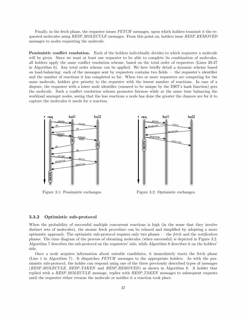
Finally, in the fetch phase, the requester issues FETCH messages, upon which holders transmit it the re-quested molecules using RESP MOLECULE messages. From this point on, holders issue RESP REMOVEDmessages to nodes requesting the molecule.
Pessimistic conflict resolution. Each of the holders individually decides to which requester a moleculewill be given. Since we want at least one requester to be able to complete its combination of molecules,all holders apply the same conflict resolution scheme, based on the total order of requesters (Lines 20-27in Algorithm 6). Any total order scheme can be applied. We here briefly detail a dynamic scheme basedon load-balancing: each of the messages sent by requesters contains two fields — the requester’s identifierand the number of reactions it has completed so far. When two or more requesters are competing for thesame molecule, holders give priority to the requester with the lowest number of reactions. In case of adispute, the requester with a lower node identifier (ensured to be unique by the DHT’s hash function) getsthe molecule. Such a conflict resolution scheme promotes fairness while at the same time balancing theworkload amongst nodes, seeing that the less reactions a node has done the greater the chances are for it tocapture the molecules it needs for a reaction.
Figure 3.1: Pessimistic exchanges. Figure 3.2: Optimistic exchanges.
3.3.2 Optimistic sub-protocol
When the probability of successful multiple concurrent reactions is high (in the sense that they involvedistinct sets of molecules), the atomic fetch procedure can be relaxed and simplified by adopting a moreoptimistic approach. The optimistic sub-protocol requires only two phases — the fetch and the notificationphases. The time diagram of the process of obtaining molecules (when successful) is depicted in Figure 3.2.Algorithm 7 describes the sub-protocol on the requesters’ side, while Algorithm 8 describes it on the holders’side.
Once a node acquires information about suitable candidates, it immediately starts the fetch phase(Line 1 in Algorithm 7). It dispatches FETCH messages to the appropriate holders. As with the pes-simistic sub-protocol, the holder can respond using one of the three previously described types of messages(RESP MOLECULE, RESP TAKEN and RESP REMOVED) as shown in Algorithm 8. A holder thatreplied with a RESP MOLECULE message, replies with RESP TAKEN messages to subsequent requestsuntil the requester either returns the molecule or notifies it a reaction took place.
37

Algorithm 5: Pessimistic sub-protocol: requester.
1 on event combination found2 QueryPhase(combination)
3 on event response received4 if phase = query then5 QueryPhaseResp(resp mol)
6 else if phase = commitment then7 CommitmentPhaseResp(resp mol)
8 else if phase = fetch then9 FetchPhaseResp(resp mol)
10 begin QueryPhase(combination)11 phase⇐ query12 foreach molecule in combination do13 dispatch QUERY(molecule)
14 begin QueryPhaseResp(resp mol)15 if resp mol 6= RESP OK then16 Abandon(combination)
17 else if all responses have arrived then18 CommitmentPhase(combination)
19 begin CommitmentPhase(combination)20 phase⇐ commitment21 foreach molecule in combination do22 dispatch COMMITMENT(molecule)
23 begin CommitmentPhaseResp(resp mol)24 if resp mol 6= RESP OK then25 Abandon(combination)
26 else if all responses have arrived then27 FetchPhase(combination)
28 begin FetchPhase(combination)29 phase⇐ fetch30 foreach molecule in combination do31 dispatch FETCH(molecule)
32 begin FetchPhaseResp(resp mol)33 add resp mol to reaction args34 if all responses have arrived then35 Reaction(reaction args)
36 begin Abandon(combination)37 phase⇐ none38 foreach molecule in combination do39 dispatch GIVE UP(molecule)
Algorithm 6: Pessimistic sub-protocol: holder.
1 on event message received2 if message = GIVE UP then3 remove sender from molecule.list
4 else if message.molecule does not exist then5 reply with RESP REMOVED
6 else if message = FETCH then7 clear molecule.list8 reply with molecule
9 else if molecule has a commitment then10 reply with RESP TAKEN
11 else if message = QUERY then12 add sender to molecule.list13 reply with RESP OK
14 else if message = COMMITMENT then15 SortRequesters(molecule)16 if molecule.locker = sender then17 reply with RESP OK
18 else19 reply with RESP TAKEN
20 begin SortRequesters(molecule)21 foreach pair of requesters in molecule.list do22 if req j.no r < req i.no r then23 put req j before req i24 continue
25 if req j.id < req i.id then26 put req j before req i
27 molecule.locker ⇐ molecule.list (0)
38

If the requester acquires all of the molecules, the reaction is subsequently performed, and the requestersends out REACTION messages to holders to notify them the molecules are being consumed. This causesholders to reply with RESP REMOVED messages to subsequent requests from other requesters. In case therequester received a RESP REMOVED or a RESP TAKEN message, it aborts the reaction and returns theobtained molecules by enclosing them in GIVE UP messages, which allows holders to give them to others.
Optimistic conflict resolution. Given the fact that the optimistic sub-protocol is designed to be executedby nodes in a highly reactive stage, there is no need for a strict conflict resolution policy. Instead, the nodethe request of which first reaches a holder obtains the desired molecule. However, the optimistic sub-protocoldoes not ensure that a reaction will be performed in case of a conflict. In the worst case, all attempts atfetching molecules might be aborted, for instance when three nodes try to fetch three molecules A,B and C,each node trying to get two of them in a cyclic way: a situation where N1 succeeds to fetch A, N2 succeedsto fetch B and N3 succeeds to fetch C, will inevitably lead to a general abort.
Algorithm 7: Optimistic sub-protocol: requester.
1 on event combination found2 foreach molecule in combination do3 dispatch FETCH(molecule)
4 on event response received5 if response 6= RESP MOLECULE then6 Abandon(combination)7 return
8 add response.molecule to reaction args9 if all responses have arrived then
10 NotifyHolders(combination)11 Reaction(reaction args)
12 begin NotifyHolders(combination)13 foreach molecule in combination do14 dispatch REACTION(molecule)
15 begin Abandon(combination)16 foreach molecule in combination do17 dispatch GIVE UP(molecule)
Algorithm 8: Optimistic sub-protocol: holder.
1 on event message received2 if message = GIVE UP then3 molecule.state⇐ free
4 else if message = REACTION then5 remove molecule
6 else if message.molecule does not exist then7 reply with RESP REMOVED
8 else if molecule.state = taken then9 reply with RESP TAKEN
10 else11 molecule.state⇐ taken12 reply with RESP MOLECULE
3.3.3 Sub-protocol mixing
During its execution, a program typically passes through two different stages. The first one is the highlyreactive stage, which is characterised by a high volume of possible concurrent reactions. In such a scenario,the use of the pessimistic sub-protocol would lead to superfluous network traffic, since the probability of areaction’s success is rather high. Thus, the optimistic approach is enough to deal with concurrent accesses tomolecules. The second stage is the quiet stage, when there is a relatively small number of possible reactions.Since this entails highly probable conflicts between nodes, the pessimistic sub-protocol has to be employedin order to ensure the liveness of the system. Thus, the execution environment has to be able to adapt tochanges and switch to the desired protocol accordingly. Moreover, these protocols have to be able to coexistin the same environment, as different nodes may act according to a different protocol at the same time.
Switching. Ideally, the execution environment could be perceived as a whole in which the switch happensunanimously and simultaneously. Obviously, a global view of the reaction potential cannot be maintainedin a large-scale system. Instead, each node independently decides which sub-protocol to employ for eachreaction. The decision is first based on a node’s local success rate, denoted σlocal, computed on the basis ofthe success history of the last queries the node issued. In order not to base the decision only on its local
39

observations, a node also keeps track of local success rates of other nodes; each time a node receives a requestor a reply message, the sender supplies it with its own current history-based success rate, stored into a list (oftunable size). Note that when there are multiple rules being executed, the node takes into account only theinformation relevant to the rule it is currently executing. We denote σ the overall success rate, computed asthe weighted arithmetic mean of a node’s local success rate and the ones collected from other nodes. Finally,the decision as to which protocol to employ depends on the rule a node wishes to execute. More specifically,it is determined by the arity of a rule, since the more molecules the rule needs, the harder it is to assurethey will all be obtained. To grab r molecules, a node employs the optimistic sub-protocol if and only ifσr ≥ s, where r is the number of arguments the chosen rule has and s is a predefined threshold value. Ifthe inequality is not satisfied, the node employs the pessimistic sub-protocol. Even though a more in-depthdiscussion about the value of the switch threshold falls out of the scope of the present work, we show itsinfluence on the protocol’s performance in Section 3.4.
Coexistence. Due to the locality of the decision of switching between sub-protocols, not all participantsin the system will perform it in the exact same moment, leading to a state where some nodes try to grabthe same molecules using different sub-protocols. In order to distinguish between optimistic and pessimisticrequests, each requester incorporates a request type field into messages. Based on this field, the node holdingthe conflicting molecule gives priority to nodes employing the more conservative, pessimistic algorithm, soas not to jeopardise pessimistic protocol’s liveness. More concretely, let O and P two nodes, respectivelyoptimistic and pessimistic, trying to fetch the same molecule M from holder H. We can distinguish two cases:Firstly, if M receives O’s FETCH message before P ’s QUERY message, O will receive the molecule and Pwill receive RESP TAKEN, making it give up the reaction right away. In the inverse scenario, P is insertedin the list of requesters for M . If O’s FETCH message reaches H before P ’s subsequent COMMITMENTmessage, O’s message will be set back temporarily waiting for the end of the pessimistic round initiatedby P . Doing so ensures that a pessimistic node (P or another node in M ’s requester list) will be able tograb the molecules it needs eventually, by preventing O (or any other optimistic node) to interfere in thepessimistic protocol.
3.3.4 Dormant nodes
During the quiet stage, the system might reach a point where n � m (n denotes the number of nodes inthe system, while m represents the number of molecules). In this extreme scenario, having many nodesrepresents a burden for the system, as most of the requests sent for molecules will ultimately be rejectedby holders, elevating the network traffic without speeding up the progression of the computation. Thus weintroduce the notion of dormant pessimistic nodes — nodes which are using the pessimistic sub-protocol tocapture molecules, but do so less often than usual. When a node switches to the pessimistic sub-protocol,it starts counting the number of consecutively aborted reactions. Once this number reaches a threshold a,it puts itself to sleep for a predefined amount of time δ — it becomes a dormant node. It then wakes upand tries to capture another combination of molecules. In case it succeeds, it becomes an active pessimisticnode again. Otherwise, it returns to the dormant state for another δ amount of time, and so forth. In orderto avoid massive awakenings of nodes, i.e. the simultaneous resumption of activities of a large number ofdormant nodes, we allow the actual amount of time a node spends as dormant to vary by a constant εδ fromδ: before putting itself to sleep, a node randomly chooses the number of steps it is going to sleep for fromthe interval [δ − εδ, δ + εδ]. Dormant nodes do not put their entire execution on hold — they are still activein the system as molecule holders. Note that a discussion about concrete values of δ, εδ and a and theirfine-tuning is here out of scope.
3.3.5 Multiple-rules programs
Thus far we focused on the protocol and its various aspects carrying the assumption that there is only onerule in the program. We need to extend the protocol to programs with multiple rules. As every node triesto carry out reactions, when multiple rules are present, each of them has to decide which of the rules it is
40
going to employ in a given cycle. Recall n denotes the number of nodes. Let nr � n be the number ofrules. We refer to the rule being executed by a node at a given moment as its active rule. While decidingwhich of the sub-protocols to employ, a node should take into account exclusively the capture attempts madewhile executing the active rule. Thus, the calculation of the success rate is adapted as follows: each nodemaintains multiple success rates σi, one per rule i, and bases its switch decision on the relevant one. Notethat this requires to expand the exchanged messages with one more field, namely the identifier of the rulefor which the success rate is contained in the message.
Initial rule assignment. Nodes pick randomly one of the rules in the program with which to start theexecution, except nr nodes that are each permanently assigned a different rule. These rule keepers canbe selected based on the hash identifiers assigned to the rules: a node is the rule keeper for a rule if thenode identifier is numerically the closest to the rule’s hash identifier. In case a node, according to the hashfunction, should be the rule keeper for more than one rule, it may delegate the responsibility for all but oneof them to other randomly-selected nodes. Rule keepers try to execute their assigned rules all throughoutthe computation — they behave as if only one rule (the one they execute) is present in the system.
Changing the active rule. The reaction potential of a rule varies throughout the computation; dependingon the state of the program at a given moment, more reactants may be present for one rule than another.Thus, nodes ought to be able to change their active rules during the execution based on the reaction potentialof the rules. While a node is trying to obtain molecules using the optimistic sub-protocol, a change of theactive rule is not being considered, as using this sub-protocol is an indicator of the active rule’s high reactionpotential. Hence, a change may occur when and only when a node is employing the pessimistic sub-protocol.A node changes its active rule if the following conditions are met:
1. the node is currently using the pessimistic sub-protocol;
2. the node did not succeed to perform a reaction in the previous cycle;
3. the success rate for the active rule observed by the node is the smallest amongst all rules’ observedsuccess rates.
The node then switches for the rule with the highest success rate known, If the current σi value of the newlyselected active rule i permits the node to employ the optimistic protocol, it resets its grab history and setsσi to 1, since it means that its reaction potential is high, entailing a fair amount of reactions to be donewith this rule. If even the new active rule’s reaction potential is low, the node will become a dormant nodeimmediately after changing its active rule. When it wakes up, it will start trying to apply the new activerule pessimistically.
3.3.6 Protocol’s safety and liveness
A capture protocol needs to satisfy the two following properties:
• safety : a molecule is used in at most one reaction (we consider that every reaction consumes all of themolecules entering it);
• liveness: if at least one reaction is continuously possible, a reaction is performed in a finite time.
Theorem 3. A molecule is consumed in at most one reaction.
Proof. Let us concentrate first on the optimistic case (Algorithms 7 and 8) and assume by contradiction thata molecule is consumed twice. It follows that the same molecule was captured by at least two nodes. This inturn means that a RESP MOLECULE message was sent by the holder to these two nodes for this molecule.This message can be sent only in case the molecule’s state is free. A molecule cannot be in the free state
41
after being sent except in case the requester which obtained it finally abort the reaction and sends it backto the holder. It is consequently impossible for two nodes to obtain the same molecule at the same time.
Let us now consider the pessimistic case (Algorithms 5 and 6). Similarly assume by contradiction thattwo pessimistic nodes obtain the same molecule. It follows that they both entered the fetch phase, and thatconsequently, prior to that, they both received a COMMITMENT message sent by the holder. This meansthat both nodes were ranked first by the SortRequesters() function which can be true only if both nodesare not in the list of requesters for this molecule at the same time. Once one node enters the list, it can beremoved from the list only upon reaction or if it abandons the reaction, making it impossible for the secondnode to be ranked first and thus obtain molecule if it was not either sent back to the holder or consumed inthe reaction and removed on the holder’s side. A contradiction.
Finally, there are two cases of conflict between the two protocols. Following our argument about thecoexistence of the protocol, we see that when an optimistic request arrives before a pessimistic one, thepessimistic request is aborted because the molecule has already been reserved by the optimistic requester.On the other hand, if a pessimistic request arrives first, the optimistic request is aborted in favour of thepessimistic one.
Theorem 4. If at least one reaction is continuously possible, one reaction is performed in a finite time.
Proof. Let us first remark that under the assumptions that nodes are reliable and links are reliable FIFOchannels, the protocol is deadlock-free. We can observe from algorithms that a requester will always get aresponse for each sent request. Based on the received responses, it will either perform the reaction or abortit and continue its execution, i.e., retry to fetch molecules.
If at least reaction is possible, then it means that there exists a multiset M of molecules that is reactive,i.e., matches the pattern and satisfies the condition of a rule.
Initially, nodes are all optimistic. In this configuration, either some node actually perform some reactionor all attempt at fetching molecules fail until all nodes switch for the pessimistic protocol (which necessarilyarrives in a finite time in this case as optimistic nodes continuously try to fetch molecules and decreasestheir σ in case of failures.
Once all nodes are pessimistic, either part of the molecules in M are consumed, which means a reactionoccurred, or M remains complete until the molecules in M constitutes the only reactants left in the solution.In the latter case, at least the rule keeper rk for this reaction will try to grab the molecules (we assumea perfect discovery protocol). Either it is alone trying to grab the molecules in which case it will actuallysucceed, or it is not. In this last case, either rk or another one succeeds to grab the molecules (due to thepessimistic resolution scheme) and perform the reaction.
3.4 Evaluation
Our protocol was simulated in order to better capture its performance. We developed a Python-based,discrete-time simulator, including a DHT layer performing the random dissemination of a set of moleculesover the nodes, on top of which the capture protocol was implemented. The simulator adopted a discrete-timeapproach: any message issued at time t is received and processed by the destination node at time t+1. Also,after a reaction is performed or aborted at time t, the node tries to fetch another set of reactants. Unlessotherwise noted, all presented experiments simulate a system of 250 nodes trying to execute a chemicalprogram containing a solution with 15000 molecules.
The reactions’ durations are assumed negligible, as our goal is to evaluate the capture protocol itself. Forall of the simulations, we set the threshold between optimism and pessimism at s = 0.7, and the followingvalues for constants related to dormant nodes: a = 10; δ = 20; εδ = 4. Figures presented below show thevalues obtained by averaging result data over 50 runs. As the deviation for each simulation is negligible, wekept only the averaged values.
42
There are two sets of experiments. In the first one, we tested the protocol’s behaviour, its performanceand the network traffic generated by a simple program with a single rule. The second set of experimentsexamines the system’s behaviour when executing programs with multiple rules. We simulated five differentprograms on top of the protocol. Note that the programs do not represent concrete implementations ofapplications since the actual reactions and their results are not taken into account. Rather, they wereconceived in such a way as to examine the protocol in detail.
3.4.1 Single-rule experiments
In the first set of experiments we focused on the characteristics of the protocol itself, namely the performanceand network overhead of each sub-protocol and the switch between them. Thus, the single-rule program wasused throughout this set of experiments. It consists only of a simple rule which consumes two moleculeswithout producing anything.
Experiment 1 (execution time). Firstly we evaluate separately the performance characteristics of bothsub-protocols. Figure 3.3 shows the averaged number of reactions left to execute at each step, until inertia,using only the optimistic mode, only the pessimistic mode, and the complete protocol with switches betweenprotocols (using s = 0.7), with and without the optimisation of dormant nodes, respectively. The theoreticoptimum curve represents the amount of steps needed to complete the execution in an ideal distributedsystem, i.e., with the highest possible parallelism degree and no conflicts during the whole computation:Considering that we need at least two steps to fetch molecules (one to request them and one to receivethem), this hypothetical ideal system needs 2 ∗ m
nr steps to complete, where m is the number of molecules,n the number of nodes and r the arity of the rule. This represents a lower bound on the number of steps,regardless of the model of computation, be it chemical or not. Note that a logarithmic scale is used for thenumber of reactions left. The figure shows that, when using only the optimistic protocol, there is a strongdecline in the number of reactions left at the beginning of the computation, i.e., when a lot of reactionsare possible and thus there are only few conflicts. While this number declines, it gets harder for nodes tograb molecules, up to the point where the system is not able to move forward in the computation, as thefew reactions left constantly generate conflicts and prevent termination. When the nodes are all pessimistic,there is a steady, linear decrease in the number of reactions left. The system is able to reach inertia, thanks tothe liveness property of the pessimistic protocol. For most steps, the mixed curve traces the exact same pathas the optimistic one, which means that during this period the nodes employ the optimistic sub-protocol.Towards the end, the system is able to quickly finish the execution as an aftermath of switching to thepessimistic sub-protocol. After the switch, it diverges from the optimistic curve to mimic the pessimisticone, exhibiting a 42% performance boost compared to the performance of the pessimistic sub-protocol.Comparing the theoretic optimum to our protocol, we notice an increase of 166% in the number of stepsneeded to reach inertia, which is not very conclusive, and can be seen as the cost of distributed coordination.Finally, as far as performance is concerned, including dormant nodes leads to similar results.
Experiment 2 (Switch threshold impact). Next, we want to assess the impact of the switch thresholds on the overall performance of the system. Figure 3.4 depicts, in the same logarithmic scale, the number ofreactions left after each step for different threshold values, varying from 0.1 to 0.9. As suspected, the curvesoverlap during most steps, most nodes employing the optimistic sub-protocol. The first curve to diverge isthe one where the switch threshold is set very high, to s = 0.9. Because the system depicted by that curvedid not fully exploit the optimistic sub-protocol, it is the last to finish the execution. Conversely, a lowvalue for s can lead to avoidable yet costly conflicts and impact negatively the performance of the execution.Although slightly, besides the one for s = 0.9, the curves start diverging at different moments, and, thus,complete the execution after a different number of steps. Figure 3.4 shows that, out of the five values testedfor the switch threshold, s = 0.7 yields the best performance results in this particular scenario. Finding theoptimal value for any application falls out of the scope of this study.
43

0.01
0.1
1
10
100
1000
10000
0 50 100 150 200 250 300 350 400 450 500
Re
ac
tio
ns
left
Time (in steps)
DormantMixed
PessimistOptimist
Theoretic Optimum
Figure 3.3: Performance of protocol’s variants.
0.01
0.1
1
10
100
1000
10000
0 20 40 60 80 100 120 140 160 180 200
Re
ac
tio
ns
left
Time (in steps)
s = 0.1s = 0.3s = 0.5s = 0.7s = 0.9
Figure 3.4: Influence of the switch threshold.
0
50
100
150
200
250
300
0 20 40 60 80 100 120 140 160
Nu
mb
er
of
no
de
s
Time (in steps)
OptimistsPessimistsDormant
Figure 3.5: Evolution of the node population.
0
200
400
600
800
1000
1200
1400
1600
0 1 2 3 4 5 6 7 8 9 10
Sw
itc
he
s p
er
ste
p
Number of nodes (x1000)
Switch speed
Figure 3.6: Switch speed.
Experiment 3 (Switch behaviour). Here we examine the behaviour of the process of switching fromone protocol to the other. Figure 3.5 depicts the evolution of the number of nodes in each mode during theexecution. We can see that, at the beginning of the execution, all of the nodes start grabbing molecules byusing the optimistic sub-protocol. About half way through the execution, optimistic nodes start abortingmore and more reactions, so they switch to the pessimistic sub-protocol. We observe that, thanks to thesystematic exchanges of local σ values, nodes in the system reach a global consensus rather quickly — for asystem with 250 nodes, at most 15 steps are needed for all of the nodes to switch to the pessimistic protocol.For the following 15 steps all of the nodes are active – and pessimistic – and try to capture molecules.However, as the concentration of molecules further drops, the number of dormant nodes increases, in thisway reducing network traffic and allowing the still active nodes to capture the wanted molecules with moreease. Note that, while the overall number of dormant nodes increases, nodes wake up after a certain periodand become pessimistic again. Figure 3.6 illustrates the number of nodes that switch from the optimisticto the pessimistic sub-protocol at each step during the transition period. One can observe that the morenodes in the system, the greater the number of nodes that switch per step. This behaviour comes from thefact that an increase in the number of nodes implies a greater accuracy of the system’s state estimation σ aseach node communicates with a wider spectre of nodes. This shows that the system, regardless of its size,can react quickly to changes, even though there is no global view of the situation.
Experiment 4 (communication costs). Next, we investigate the communication costs involved in theprocess. Figures 3.7, 3.8, 3.9 and 3.10 depict the number of messages sent per cycle in a system of 250 nodes.By cycle, we here means 12 simulation steps, as it is the lowest common multiple of 4 and 6; at most 4steps are needed for the optimistic sub-protocol to complete, and at most 6 for the pessimistic sub-protocol.
44

Figure 3.7: Number of messages when using the opti-mistic sub-protocol only.
Figure 3.8: Number of messages when using the pes-simistic sub-protocol only.
Figure 3.9: Number of messages when using the pro-posed protocol (without the dormant state).
Figure 3.10: Number of messages when using theproposed protocol (with the dormant state).
The messages are classified into two categories: useful messages (ones which led to a reaction, in black) anduseless messages (those which did not induce a reaction, in grey). When looking at the communication costswhen only the optimistic sub-protocol is used (Figure 3.7), one can observe that a high volume of reactions isdone in the beginning of the execution with a small percentage of conflicts, and thus a small amount of uselessmessages. However, as the execution progresses, the percentage of useful messages drops rapidly, while thetotal number of messages is kept high. Figure 3.8 shows that the exclusive use of the pessimistic sub-protocolconsumes less messages, with the percentage of useful messages dropping steadily and slowly. At the sametime, as there are less and less molecules in the system, the total number of messages slowly grows beforepeaking at around 8000 messages per cycle and then rapidly decreasing towards the end of the execution.When comparing Figure 3.9 to the previous two, we note again that the full protocol takes over the bestproperties of both of its sub-protocols: an elevated number of useful messages at optimistic times and adecrease in the total number of messages at pessimistic ones. A decrease of 30% in the number of messagescan be observed when compared to the pessimistic sub-protocol alone. In addition, Figure 3.10 reveals thatusing the policy of dormant nodes further improves the scalability of the protocol, as it significantly reducesthe total number of messages towards the end of the execution where there is the highest potential numberof conflicts.
45

3.4.2 Multiple-rules experiments
In order to examine the behaviour of the rule-changing mechanism described earlier, we conducted a set ofexperiments with several multiple-rule programs. One of them was the simple split-merge workflow illustratedin Figure 3.11. It consists of four rules: R0, R1, R2 and R3. The rule R0 consumes two molecules of typeT0 and produces two molecules: one of type T1, the other of type T2. These are used as input by R1 andR2, respectively. These rules can, thus, be run concurrently and independently of each other. R1 producesone molecule of type T3, while R2 produces one of type T4. Finally, their outputs are merged by the ruleR3, which consumes one molecule per type — T3 and T4 — and produces no output.
Figure 3.11: A rule-based workflow program. 0
50
100
150
200
250
300
0 50 100 150 200 250 300N
um
be
r o
f n
od
es
Time (in steps)
R0R1R2R3
Figure 3.12: Number of nodes executing each rule.
0
50
100
150
200
250
300
0 50 100 150 200 250 300
Nu
mb
er
of
no
de
s
Time (in steps)
OptimistsPessimistsDormant
Figure 3.13: Number of nodes in each mode.
0.01
0.1
1
10
100
1000
10000
100000
0 50 100 150 200 250 300
Nu
mb
er
of
no
de
s
Time (in steps)
T0T1T2T3T4
Figure 3.14: Number of molecules of each type (loga-rithmic scale).
The results of the execution of these programs are depicted in Figures 3.12—3.14. The rule-changingpattern reveals that the nodes first massively execute R0 until the concentration of T0-molecules drops belowthose of T1- and T2-molecules. The nodes then distribute themselves over the rules in such a way as toconsume mostly these molecules — around 100 nodes per rule for R1 and R2. As they produce T3- andT4-molecules, about 50 nodes start executing the last rule, R3. As T1- and T2-molecules are consumed at afaster pace, nodes start abandoning R1 and R2 and pick R3. All the while, most of the nodes are employingthe optimistic sub-protocol. Then, in between steps 200 and 250 about half of the nodes change back toR1 and R2 in order to consume the remaining T1- and T2-molecules, respectively, causing a decrease inthe number of optimists, due to the globally low concentration of molecules. At the end of the executionalmost all of the nodes use R3, most of them being dormant. Indeed, as there are only a few reactions leftat that point, it is impossible for most of the nodes to perform reactions in spite of the fact that they have
46
correctly picked the rule to execute. This experiment shows that the rule-changing mechanism is able tofollow the dependency patterns of a program with multiple rules. Moreover, we can see that during most ofthe execution the majority of nodes uses the optimistic sub-protocol, confirming that the protocol is able toadapt itself to the current situation in the system.
Experiments were conducted with other programs containing different dependency patterns. Please referto the journal article [17] for the whole set of results we obtained.
3.5 Conclusion
This chapter proposed and validated the fundamental building block of our future distributed chemical ma-chine: the atomic capture protocol. This protocol assumes molecules are already known by the nodes tryingto capture them. A missing element towards a distributed chemical machine is the discovery mechanism.Another aspect ignored in this chapter is the detection of termination. While we studied it without any no-tion of decentralisation in Chapter 2, we now need to make the detection happen in distributed settings. Thenext chapter is about filling these two gaps, the implementation and experimental evaluation of a softwareprototype of a distributed chemical machine.
47


Chapter 4
Implementing Distributed Chemical Machines
This chapter describes two distributed chemical machines we have designed, developed and experimented inreal settings, over the Grid’5000 platform. The first one is shaped as a hierarchical reactor where reactionsstart at the leaves of a tree of compute nodes, and where inert subsolutions are then merged and reactivated asthey move up the hierarchy until reaching the top level, the root of the tree. The second one fully decentralizesthe discovery, capture and reactions of molecules, building a flat reactor. This second reactor supports thehigher-order.
Joint work with:
? Marko Obrovac (PhD student, Inria)
4.1 The need for chemical run-time environments
Despite a large spectrum of applications (see [10] for an overview of them), the chemical model severelysuffers from a lack of means for its execution over large-scale platforms and yet executing chemical programsis crucial on the road to its adoption in real contexts. This is particularly true in regard to its potentialuse in the specification of service coordination, to be detailed in Chapters 5 and 6. Without a distributedchemical machine able to execute the coordination, such works remain conceptual. In other words, we wantto build a machine able to execute any chemical specification over large scale platforms, transparently forthe programmer.
In [12], to introduce the philosophy of chemical programming, Banatre and Le Metayer distinguishedlogical parallelism from physical parallelism:
Physical parallelism is related to the implementation; it corresponds to the distribution of taskson several processors. By logical parallelism, we mean the possibility of describing a program as acomposition of several independent tasks. Of course, a particular implementation can turn logicalparallelism into physical parallelism, but these notions have very different natures: the former isa program-structuring tool, whereas the latter is an implementation technique.
It appears that this distinction holds for distribution as well: reactions are implicitly local and au-tonomous. Time has come to offer an implementation to the chemical model, in other words, to turn itslogical parallelism and distribution into physical ones. While the chemical model has been implemented overparallel machines (we review these works in the following), this has not been the case on more distributedplatforms.
49
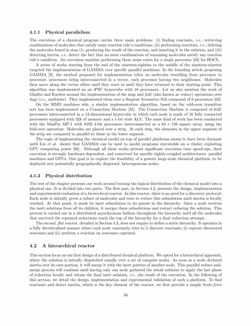
4.1.1 Physical parallelism
The execution of a chemical program carries three main problems: (i) finding reactants, i.e., retrievingcombinations of molecules that satisfy some reaction rule’s conditions, (ii) performing reactions, i.e., deletingthe molecules found in step (i), producing the result of the reaction, and inserting it in the solution, and (iii)detecting inertia, i.e. detect the fact that no more combinations of remaining molecules satisfy any reactionrule’s condition. An execution machine performing these steps exists for a single processor [83] for HOCL.
A series of works starting from the end of the nineteen-eighties to the middle of the nineteen-ninetiestargeted the implementation of GAMMA over specific parallel machines: In the founding article proposingGAMMA [9], the method proposed for implementation relies on molecules travelling from processor toprocessor, processors being interconnected in a vector, each processor having two neighbours. Moleculesthen move along the vector either until they react or until they have returned to their starting point. Thisalgorithm was implemented on an iPSC hypercube with 16 processors. Let us also mention the work ofGladitz and Kuchen around the implementation of the map and fold (also known as reduce) operations overbags (i.e., multisets). They implemented them over a Sequent Symmetry S16 composed of 6 processors [63].
On the SIMD machines side, a similar implementation algorithm, based on the odd-even transitionsort has been implemented on a Connection Machine [35]. The Connection Machine is composed of 64Kprocessors interconnected in a 12-dimensional hypercube in which each node is made of 16 fully connectedprocessors equipped with 32k of memory and a 1-bit wide ALU. The same kind of work has been conductedwith the MasPar MP-1 with 8192 4-bit processors interconnected as a 64 × 128 square array, using thefold-over operation: Molecules are placed over a strip. At each step, the elements in the upper segment ofthe strip are compared in parallel to those in the lower segment.
The topic of implementing the chemical model on top of parallel platforms seems to have been dormantuntil Lin et al. shown that GAMMA can be used to model programs executable on a cluster exploitingGPU computing power [66]. Although all these works present significant execution time speed-ups, theirexecution is strongly hardware-dependent, and conceived for specific tightly-coupled architectures: parallelmachines and GPUs. Our goal is to explore the feasibility of a generic large-scale chemical platform, to bedeployed over potentially geographically dispersed, heterogeneous nodes.
4.1.2 Physical distribution
The rest of the chapter presents our work around turning the logical distribution of the chemical model into aphysical one. It is divided into two parts. The first part, in Section 4.2, presents the design, implementationand experimental evaluation of a hierarchical reactor. In this reactor, there is no need for a discovery protocol:Each node is initially given a subset of molecules and tries to reduce this subsolution until inertia is locallyreached. At that point, it sends its inert subsolution to its parent in the hierarchy. Once a node receivesthe inert solutions from all its children, it merges these subsolutions and restart reducing the solution. Thisprocess is carried out in a distributed asynchronous fashion throughout the hierarchy until all the moleculesthat survived the repeated reductions reach the top of the hierarchy for a final reduction attempt.
The second, flat reactor, detailed in Section 4.3, does not require to define a static hierarchy. It operates ina fully decentralized manner where each node constantly tries to i) discover reactants, ii) capture discoveredreactants and iii) perform a reaction on reactants captured.
4.2 A hierarchical reactor
This section focus on our first design of a distributed chemical platform. We opted for a hierarchical approach,where the solution is initially dispatched equally over a set of compute nodes. As soon as a node declaredinertia over its own portion, it will merge it with the inert portion of another node. This parallel reduce-and-merge process will continue until having only one node gathered the whole solution to apply the last phaseof reduction locally and obtain the final inert solution, i.e., the result of the execution. In the following ofthis section, we detail the design, implementation and experimental validation of such a platform. To findreactants and detect inertia, which is the key element of the reactor, we first provide a simple brute-force
50
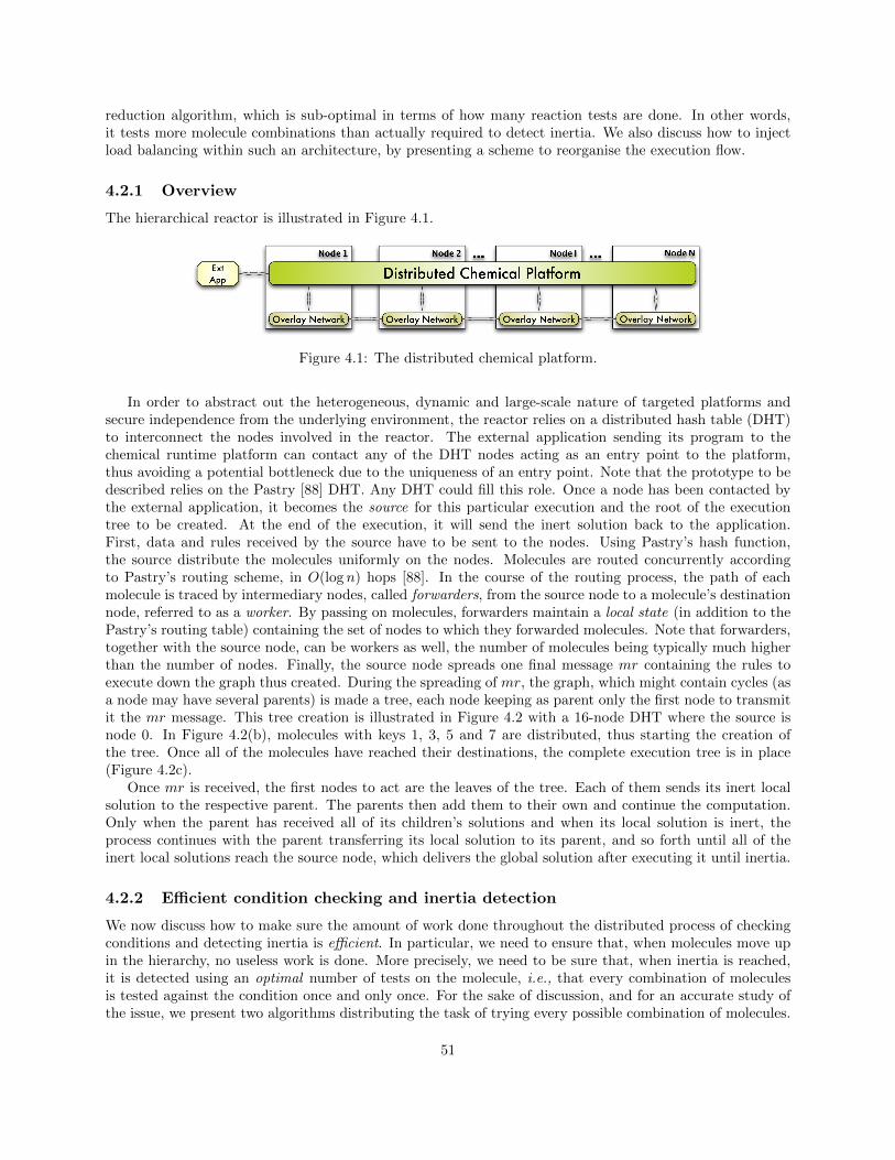
reduction algorithm, which is sub-optimal in terms of how many reaction tests are done. In other words,it tests more molecule combinations than actually required to detect inertia. We also discuss how to injectload balancing within such an architecture, by presenting a scheme to reorganise the execution flow.
4.2.1 Overview
The hierarchical reactor is illustrated in Figure 4.1.
Figure 4.1: The distributed chemical platform.
In order to abstract out the heterogeneous, dynamic and large-scale nature of targeted platforms andsecure independence from the underlying environment, the reactor relies on a distributed hash table (DHT)to interconnect the nodes involved in the reactor. The external application sending its program to thechemical runtime platform can contact any of the DHT nodes acting as an entry point to the platform,thus avoiding a potential bottleneck due to the uniqueness of an entry point. Note that the prototype to bedescribed relies on the Pastry [88] DHT. Any DHT could fill this role. Once a node has been contacted bythe external application, it becomes the source for this particular execution and the root of the executiontree to be created. At the end of the execution, it will send the inert solution back to the application.First, data and rules received by the source have to be sent to the nodes. Using Pastry’s hash function,the source distribute the molecules uniformly on the nodes. Molecules are routed concurrently accordingto Pastry’s routing scheme, in O(log n) hops [88]. In the course of the routing process, the path of eachmolecule is traced by intermediary nodes, called forwarders, from the source node to a molecule’s destinationnode, referred to as a worker. By passing on molecules, forwarders maintain a local state (in addition to thePastry’s routing table) containing the set of nodes to which they forwarded molecules. Note that forwarders,together with the source node, can be workers as well, the number of molecules being typically much higherthan the number of nodes. Finally, the source node spreads one final message mr containing the rules toexecute down the graph thus created. During the spreading of mr, the graph, which might contain cycles (asa node may have several parents) is made a tree, each node keeping as parent only the first node to transmitit the mr message. This tree creation is illustrated in Figure 4.2 with a 16-node DHT where the source isnode 0. In Figure 4.2(b), molecules with keys 1, 3, 5 and 7 are distributed, thus starting the creation ofthe tree. Once all of the molecules have reached their destinations, the complete execution tree is in place(Figure 4.2c).
Once mr is received, the first nodes to act are the leaves of the tree. Each of them sends its inert localsolution to the respective parent. The parents then add them to their own and continue the computation.Only when the parent has received all of its children’s solutions and when its local solution is inert, theprocess continues with the parent transferring its local solution to its parent, and so forth until all of theinert local solutions reach the source node, which delivers the global solution after executing it until inertia.
4.2.2 Efficient condition checking and inertia detection
We now discuss how to make sure the amount of work done throughout the distributed process of checkingconditions and detecting inertia is efficient. In particular, we need to ensure that, when molecules move upin the hierarchy, no useless work is done. More precisely, we need to be sure that, when inertia is reached,it is detected using an optimal number of tests on the molecule, i.e., that every combination of moleculesis tested against the condition once and only once. For the sake of discussion, and for an accurate study ofthe issue, we present two algorithms distributing the task of trying every possible combination of molecules.
51
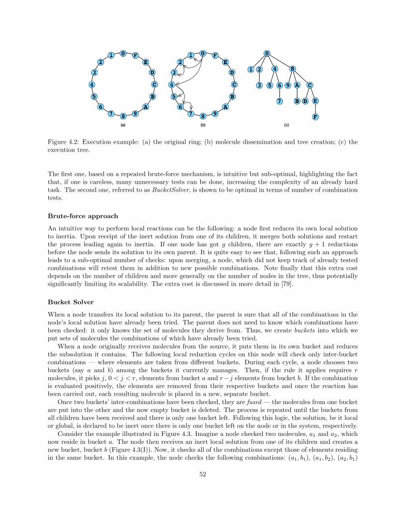
Figure 4.2: Execution example: (a) the original ring; (b) molecule dissemination and tree creation; (c) theexecution tree.
The first one, based on a repeated brute-force mechanism, is intuitive but sub-optimal, highlighting the factthat, if one is careless, many unnecessary tests can be done, increasing the complexity of an already hardtask. The second one, referred to as BucketSolver, is shown to be optimal in terms of number of combinationtests.
Brute-force approach
An intuitive way to perform local reactions can be the following: a node first reduces its own local solutionto inertia. Upon receipt of the inert solution from one of its children, it merges both solutions and restartthe process leading again to inertia. If one node has got g children, there are exactly g + 1 reductionsbefore the node sends its solution to its own parent. It is quite easy to see that, following such an approachleads to a sub-optimal number of checks: upon merging, a node, which did not keep track of already testedcombinations will retest them in addition to new possible combinations. Note finally that this extra costdepends on the number of children and more generally on the number of nodes in the tree, thus potentiallysignificantly limiting its scalability. The extra cost is discussed in more detail in [79].
Bucket Solver
When a node transfers its local solution to its parent, the parent is sure that all of the combinations in thenode’s local solution have already been tried. The parent does not need to know which combinations havebeen checked: it only knows the set of molecules they derive from. Thus, we create buckets into which weput sets of molecules the combinations of which have already been tried.
When a node originally receives molecules from the source, it puts them in its own bucket and reducesthe subsolution it contains. The following local reduction cycles on this node will check only inter-bucketcombinations — where elements are taken from different buckets. During each cycle, a node chooses twobuckets (say a and b) among the buckets it currently manages. Then, if the rule it applies requires rmolecules, it picks j, 0 < j < r, elements from bucket a and r− j elements from bucket b. If the combinationis evaluated positively, the elements are removed from their respective buckets and once the reaction hasbeen carried out, each resulting molecule is placed in a new, separate bucket.
Once two buckets’ inter-combinations have been checked, they are fused — the molecules from one bucketare put into the other and the now empty bucket is deleted. The process is repeated until the buckets fromall children have been received and there is only one bucket left. Following this logic, the solution, be it localor global, is declared to be inert once there is only one bucket left on the node or in the system, respectively.
Consider the example illustrated in Figure 4.3. Imagine a node checked two molecules, a1 and a2, whichnow reside in bucket a. The node then receives an inert local solution from one of its children and creates anew bucket, bucket b (Figure 4.3(I)). Now, it checks all of the combinations except those of elements residingin the same bucket. In this example, the node checks the following combinations: (a1, b1), (a1, b2), (a2, b1)
52
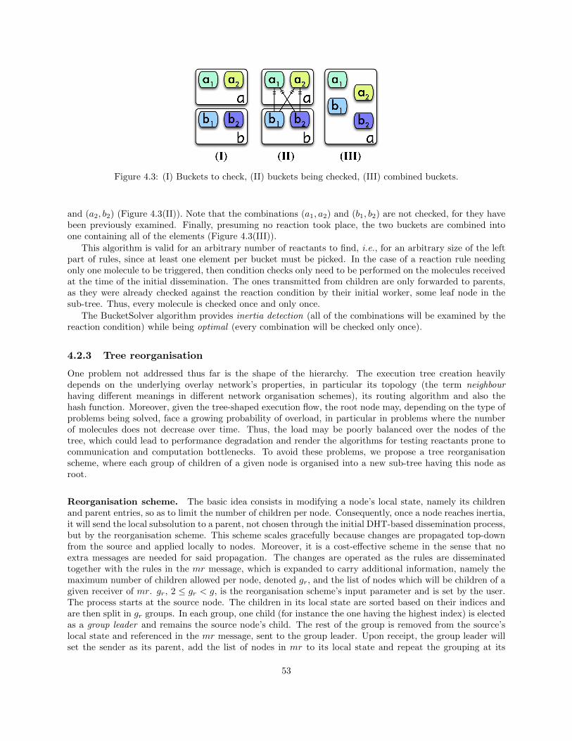
Figure 4.3: (I) Buckets to check, (II) buckets being checked, (III) combined buckets.
and (a2, b2) (Figure 4.3(II)). Note that the combinations (a1, a2) and (b1, b2) are not checked, for they havebeen previously examined. Finally, presuming no reaction took place, the two buckets are combined intoone containing all of the elements (Figure 4.3(III)).
This algorithm is valid for an arbitrary number of reactants to find, i.e., for an arbitrary size of the leftpart of rules, since at least one element per bucket must be picked. In the case of a reaction rule needingonly one molecule to be triggered, then condition checks only need to be performed on the molecules receivedat the time of the initial dissemination. The ones transmitted from children are only forwarded to parents,as they were already checked against the reaction condition by their initial worker, some leaf node in thesub-tree. Thus, every molecule is checked once and only once.
The BucketSolver algorithm provides inertia detection (all of the combinations will be examined by thereaction condition) while being optimal (every combination will be checked only once).
4.2.3 Tree reorganisation
One problem not addressed thus far is the shape of the hierarchy. The execution tree creation heavilydepends on the underlying overlay network’s properties, in particular its topology (the term neighbourhaving different meanings in different network organisation schemes), its routing algorithm and also thehash function. Moreover, given the tree-shaped execution flow, the root node may, depending on the type ofproblems being solved, face a growing probability of overload, in particular in problems where the numberof molecules does not decrease over time. Thus, the load may be poorly balanced over the nodes of thetree, which could lead to performance degradation and render the algorithms for testing reactants prone tocommunication and computation bottlenecks. To avoid these problems, we propose a tree reorganisationscheme, where each group of children of a given node is organised into a new sub-tree having this node asroot.
Reorganisation scheme. The basic idea consists in modifying a node’s local state, namely its childrenand parent entries, so as to limit the number of children per node. Consequently, once a node reaches inertia,it will send the local subsolution to a parent, not chosen through the initial DHT-based dissemination process,but by the reorganisation scheme. This scheme scales gracefully because changes are propagated top-downfrom the source and applied locally to nodes. Moreover, it is a cost-effective scheme in the sense that noextra messages are needed for said propagation. The changes are operated as the rules are disseminatedtogether with the rules in the mr message, which is expanded to carry additional information, namely themaximum number of children allowed per node, denoted gr, and the list of nodes which will be children of agiven receiver of mr. gr, 2 ≤ gr < g, is the reorganisation scheme’s input parameter and is set by the user.The process starts at the source node. The children in its local state are sorted based on their indices andare then split in gr groups. In each group, one child (for instance the one having the highest index) is electedas a group leader and remains the source node’s child. The rest of the group is removed from the source’slocal state and referenced in the mr message, sent to the group leader. Upon receipt, the group leader willset the sender as its parent, add the list of nodes in mr to its local state and repeat the grouping at its
53

Figure 4.4: Tree reorganisation example: (a) initial state, (b) first levelestablished, (c) tree completely reorganised
Figure 4.5: Software architec-ture of the hierarchical reactorprototype.
level, and so forth until reaching the bottom of the tree. The reorganisation stops once all of the nodes havereceived an mr message, which marks the beginning of the execution (using the BucketSolver algorithm).
Example. Let us demonstrate the reorganisation process on a simple example. Figure 4.4a depicts theexecution tree built after disseminating molecules with ids 0 through 8 in a 9-node system. Let node 0 be thesource node and let gr = 2. Node 0 splits its children list in two groups. It keeps node 4 from the first group(1-4) and node 8 from the second (5-8). It then sends one mr message including the list of non-leader nodesof the first group, i.e., the list 1, 2, 3, to their group leader — node 4. Another mr message containing thelist 5, 6, 7, is sent to node 8. Node 0 can now starts its execution. Concurrently, nodes 4 and 8 update theirlocal states by setting parent id = 0 and copying the respective lists they receive lists to their respectivechildren entries (Figure 4.4b). Node 4 now splits its children list into two groups (< 1, 2 > and < 3 >) andelects the leaders (2 and 3). Two mr messages are then constructed; the first one containing only 1 in itslist is sent to node 2, while the other is sent to node 3 with an empty list. Node 4 now starts the execution.Nodes 2 and 3 set their parent to 4. Node 3 starts reducing its local solution, while node 2 sends mr to node1 which sets its parent and starts the execution. The exact same effect is achieved on the right side of tree:node 8 splits its children list into two groups, sending 5 to node 6 and no list to node 7 (Figure 4.4c).
4.2.4 Prototype
To better capture the viability and performance of the hierarchical reactor, a software prototype of thearchitecture and algorithms presented above was developed1. Its components are depicted in Figure 4.5.The overlay network was implemented with FreePastry [2], an implementation developed by the originalauthors of Pastry. Its facilities are used by the two units directly above it — the central unit and the flowunit, both present on every node.
Central Unit. The central unit is the entry point of the solver, it is in charge of accepting and takingover the requests originating from external applications. It hashes the molecules and send them over toFreePastry that will actually route them to appropriate nodes. It also initiates the dissemination of the rulesby forwarding them to the flow unit which will actually perform the multicast. Once global inertia has beenachieved, it is informed by the flow unit and delivers the solution to the application.
Flow Unit. Meanwhile, each flow unit monitors the traffic in the DHT and builds its state, i.e., its viewof the execution tree, based on routing decisions taken by the overlay network. Once the disseminationprocess has completed, the flow unit holds the list of its direct tree descendants and the parent’s identity. As
1The sources are available in the branches/devel-distrib directory of the svn repository located athttp://gforge.inria.fr/scm/?group id=2125.
54

specified before, this list is used at execution time as a synchronisation barrier: the flow unit forbids sendingthe local inert solution to the parent until all of its children’s results have been received. The flow unit isalso naturally responsible for the tree reorganisation (during the rules dissemination): it elects the groupleaders, removes the rest from its children list and passes their identities on to the new group leaders.
Solver Unit. The key role in the execution is played by the solver unit, which is the implementation ofthe algorithms proposed in Section 4.2.2. The unit has two different implementations, one for each of thetwo condition checking algorithms. After the dissemination process, the central unit triggers its executionof the local solution. Once inert, the solution is transferred to the flow unit. Also, when a result froma child is received, the flow unit hands it over to the solver unit, triggering a new execution cycle. TheBucketSolver algorithm has been implemented in the solver unit in a multithreaded version: the well-definedbucket boundaries imply that two disjoint groups of buckets, each containing at least two bucket, can beprocessed independently one from the other. As a result, the solver unit implements a thread pool whichschedules the execution of groups of buckets on free threads in the pool as long as the local solution is notinert, i.e., as long as there are at least two buckets left to fuse. The synchronization this parallelizationrequires is very light. Note that such a mechanism cannot be applied to the brute-force algorithm that hasno recollection of the combinations previously checked. Parallelizing the brute-force approach would callfor a more complex synchronization, as two threads could try combinations containing the same molecule,leading to inevitably poor speed-ups.
4.2.5 Experimental evaluation
This section presents the results of an experimental evaluation of the prototype of the hierarchical reactorpresented in Section 4.2.4. The goal of this experimental campaign is fourfold: (i) examine the viability ofthe architecture, (ii) compare the reactant finding algorithms, (iii) look at the network traffic generated and(iv) test the tree reorganisation scheme laid out in Section 4.2.3. The experiments were conducted on theFrench nation-wide Grid’5000 [27] computation platform, connecting nine geographical-distant sites throughthe RENATER network2, which offers a 10 GBit/s communication channel between the sites. We varied thenumber of chemical nodes taking part in the reactor from 100 to 1000 scattered randomly across the ninesites, each Grid’5000 node hosting up to its number of cores as chemical nodes. The results represent valuesaveraged over 6 runs. The configuration of the overlay network was changed upon each run. The prototypewas tested on two chemical programs presented hereafter.
Test Programs
The evaluation of the proposed architecture and algorithms was conducted using two chemical programs.While the programs tested might seem rather simple, their interest stands in that they belong to a broaderclass of programs having a specific behaviour at run time. Even though their expression is quite simple(thanks to the uncluttered style of the chemical model), their runtime’s complexity is similar to many otherchemical programs with a more complex logic. Put simply, what matters here is the complexity of findingreactants over time. The first class of applications has a complexity that decreases over time, while thesecond exhibits a constant complexity over time.
Programs with a decreasing density. A large collection of real-world applications solve problems thecomplexity of which gradually decreases as computation progresses. In our experiments we chose to representthis class of applications with the getmax program discussed in Chapter 2. getmax is a so-called reducer rulesince each reaction decreases the total number of molecules, and consequently the density of reactants (andreactions). This is a typical scenario for many data-processing applications where the amount of data tobe processed diminishes over time. In the experiments, the getmax program was performed over a solutioninitially containing 50,000 molecules. Data processing itself was simulated through a local one-second pauseafter each reaction.
2http://www.renater.fr
55
Programs with a constant density. Our second test program is a program made of one rule acting onmolecules composed of two integers — an index and a value associated with it. The goal of the program isto sort the value through the indices. The sort rule is given below:
let sort = replace {x.i, x.v}, {y.i, y.v}by {x.i, y.v}, {y.i, x.v}if (x.i > y.i ∧ x.v < y.v) ∨ (x.i < y.i ∧ x.v > y.v)
The rule consumes two molecules if they are not already sorted in ascending order. Two new molecules arethen created, holding the same indices as the original ones, but with swapped values. Although simple, thisprogram is relevant for our experiments as it keeps the number of molecules in the solution constant — everytime two molecules are consumed, two new are created. This means that the complexity of finding reactantsremains constant throughout the execution, which allows us to better compare BucketSolver to the naiveapproach. Also, keeping constant the number of molecules and thus the amount of data, gives unbiasedinsight into possible bottlenecks and performance degradations.
Results
The four metrics evaluated so as to capture the behaviour of the hierarchical reactor prototype and verify theproperties we devised before are: (i) execution speed-up, (ii) inertia detection complexity, (iii) communicationcost and (iv) effect of tree reorganisation.
Execution speed-up. Firstly, we examined the speed-up that can be obtained using the hierarchicalreactor. Figures 4.6 and 4.7 show the speed-up in execution time achieved by comparison to the executiontime of a single executor. Using getmax (see Figure 4.6), we observe that both reactant finding algorithmsachieve significant speed-ups, linearly growing with the number of nodes. However, while the brute-forcereaches a maximum speed-up of 150, BucketSolver is able to reduce the execution time by a factor of upto 900. Although both algorithms perform the same number of reactions, when using BucketSolver, theruntime benefits from the implementation’s optimisation of multi-threading, which allows it to performmultiple reactions at a time. On the other hand, Figure 4.7 shows that in the case of the sort test programdistribution of the execution does not induce a significant speed-up. Concretely, the brute-force algorithm isbarely able to match a single instance’s execution time regardless of the number of nodes, while BucketSolverachieves speed-ups in the range 5−8. In contrast to getmax where parents in the tree have got less work to doafter receiving the results from their children, a node receives the same amount of molecules they forwardedto their children during the initial dissemination. Thus, even though the total number of molecules in thesystem is constant, the complexity of the program per active node increases over time. Consequently, parentshave got to wait longer and longer on their children’s responses as the computation is moving up in the tree,increasing the global execution time. BucketSolver still performs better due to its optimality and ability toexploit multi-threading.
Inertia Detection. Next, we wanted to experimentally verify our finding that the BucketSolver is optimalin terms of number of tests when the solution is inert. We did so using the sort program on an inert solution,i.e., an already sorted one. As expected, our observations — results are depicted in Figures 4.8 and 4.9 —were that the brute-force algorithm induced a systematically slower execution (by a factor between 4 and5 compared to BucketSolver). The exact extra-cost over BucketSolver yet fluctuated as a result of buildingdifferent execution trees for each run, due to the different overlay network’s initial configuration. Also, aspredicted, the total amount of combinations tested by BucketSolver matches that of a single executor, whilethat of the brute-force algorithm fluctuates again wildly. Finally, as already suggested by our experimenta-tions about the speed-up, the number of nodes in the case of the sort program does not greatly reduce theexecution time, suggesting that nodes spend a lot of time waiting for results from nodes in their subtree.
Let us briefly mention our experimental findings on communication overhead and the impact of the treereorganisation. These aspects are reviewed in more detail in [79]. We observed that the communicationoverhead is linear in the number of nodes and depends on the type of programs executed. In particular,
56

0
100
200
300
400
500
600
700
800
900
100 200 300 400 500 600 700 800 900 1000
Speed-u
p
Number of nodes
Brute-forceBucketSolver
Figure 4.6: Speed-up in execution time for thegetmax program.
0
1
2
3
4
5
6
7
8
9
100 200 300 400 500 600 700 800 900 1000
Speed-u
p
Number of nodes
Brute-forceBucketSolver
Figure 4.7: Speed-up in execution time for thesort program.
20
40
60
80
100
120
140
160
100 200 300 400 500 600 700 800 900 1000
Tim
e (
s)
Number of nodes
Brute-forceBucketSolver
Figure 4.8: Execution time on an inert solution(sort program).
1.2e+07
1.25e+07
1.3e+07
1.35e+07
1.4e+07
1.45e+07
1.5e+07
1.55e+07
1.6e+07
1.65e+07
1.7e+07
1.75e+07
100 200 300 400 500 600 700 800 900 1000
Num
ber
of com
bin
ations
Number of nodes
Brute-force
BucketSolver
Figure 4.9: Number of checks done on an inertsolution (sort program).
the overhead of adding new nodes is smaller for getmax since its complexity decreases over time. For bothprograms, the overhead per node decreases, showing that no bottleneck due to traffic is to be expected whenthe platform grows. Finally, our experiments involving the tree organization led us to the conclusion thatthe improvement it brings in terms of load balancing is significant, in particular on the source node: thepercentage of reactions done by the source for the sort program with 400 nodes is reduced from 65 to 25.Still, it does not bring a significant speed-up as long as the upper part of the hierarchy does not constitute abottleneck. Also, while the reorganization leads to a better load balancing, it also deepens the tree, makingpath from the leaves to the source longer.
4.3 A fully-decentralised higher-order reactor
The hierarchical reactor presented was the result of building a proof of concept of a decentralised chemicalmachine. While it constituted a significant first step, several issues were still to be solved. Firstly, decen-tralisation is still limited in the hierarchical reactor: the load on the nodes is by construction, not uniformlydispersed. In particular, a higher node in the tree is likely to experience a higher load. In other words,the hierarchical reactor suffers from its hierarchical shape. Even if all nodes apply the same algorithm,they might end up having a very different workload. Secondly, the hierarchical reactor does not guide thesearch. The molecules are randomly dispatched and moved when they cannot react any more without beingfused with other buckets. The algorithm does not search for reactants but rather checks in parallel all thecombinations in an exhaustive manner. By some simple pre-analysis of the rule, guiding the search towardsmolecules that has an actual chance of implying a reaction may significantly reduce the global complexity
57

of the reactor. Thirdly, the hierarchical reactor does not take higher-order into account. Modifying the setof enable rules dynamically is not possible. Actually, it would require a significant cost for synchronization:If some node applies a higher-order rule removing a rule, no other node should apply it anymore, calling formechanisms to inform every node of this change, such as another broadcast.
The flat reactor presented in the following addresses these problems so as to offer a fully-decentralisedplatform to execute higher-order chemical programs. Although, as the hierarchical reactor, it is based ona DHT to abstract out the details of the infrastructure, it does not build a rigid hierarchical structure todispatch and gather molecules. Instead, it builds a second DHT layer on top of the first one to store meta-data about the molecules and their state of reactiveness. Based on a specific way to order them, searchingfor reactants and detecting inertia is achieved through exploring this second layer. Once reactants are found,they still need to be acquired. This is done through the use of the adaptive capture protocol detailed inChapter 3. To make it possible to support higher-order rules, mechanisms to track a rule’s existence areincluded.
The rest of the current section is structured as follows: Section 4.3.1 presents the general executionscheme followed by a node in the flat reactor. Section 4.3.2 presents in detail how molecules are retrievedand how inertia is detected using the two-layer DHT. Section 4.3.3 presents the mechanisms enhancing thereactor with higher order. Finally the flat reactor prototype we developed is described in Section 4.3.4,and experimental results, again obtained by large deployments over the Grid’5000 platform are discussed inSection 4.3.5.
4.3.1 General execution scheme
The general idea of the underlying layers of the flat reactor is not different from the hierarchical reactordepicted in Figure 4.1. A set of nodes are interconnected into a network, each of them being equipped withthe same engine. The engine of the flat reactor is just different from the hierarchical one. We assume thatmolecules are, as within the hierarchical reactor, randomly dispatched over the nodes. The source still refersto the node initially contacted by the application that will send back the result at the end of the computation.We also assume again that the rules of the program are present in every node before nodes start trying tomake reactions.
A difference with the hierarchical reactor is that, to help discovering reactants, a second DHT layercontaining information about molecules, referred to as meta-molecules in the following, is distributed overthe nodes of the platform in an order-preserving manner. Each molecule in the first layer of the DHT isassociated with a unique meta-molecule in the second layer. This allows molecules with values within agiven range to be searched more efficiently (for instance an integer greater than 3). As we will detail laterin Section 4.3.2, each meta-molecule has a state which is either free meaning it may be used for a reaction,or inert, which denotes that a node tried to make it react but was unable to find other reactants so as tobuild a reactive combination containing it.
Algorithm 9: Main execution loop.
1 while not inert do2 meta mol1 = random mol(state = free)3 if meta mol1 = null then4 break
5 meta mol2 = find candidate(meta mol1, rule)6 if meta mol2 = null then7 meta mol1.state = inert8 store(meta mol1)9 continue
10 if grab molecules(meta mol1,meta mol2) then11 execute reaction(rule, mol1, mol2)12 store(new mol1, new mol2)13 store ack(meta new mol1, meta new mol2)14 remove(meta mol1, meta mol2)
Once molecules and rules have been dispatched,the main execution loop of every node is describedin Algorithm 9, in a simplified form as it consid-ers only one rule acting on pairs of molecules. Thealgorithm can still be easily extended to multiplerules with arities greater than 2. The loop consistsin three steps: (i) getting a random meta-moleculeor detecting inertia (lines 2—4), (ii) finding acandidate molecule it can react with (lines 5—9)and (iii) atomically grabbing the correspondingmolecules and performing the reaction (lines 10—14). Let us briefly review these three steps. Step1 (lines 2—4) initiates the loop: a node first triesto obtain a random meta-molecule, the state ofwhich is free.random mol guarantees a free meta-
58

molecule will be returned, in case one exists. If, on the other hand, no meta-molecule can be found, it meansthat, previously, another node could not find any candidate to react with the currently present molecules,implying their states were set to inert. This signals to the requesting node that inertia has been reached. Itthen stops executing the main loop (line 4).
Step 2 (lines 5—9) is triggered when a free meta-molecule has been obtained. The node now asks thesystem to find a second suitable meta-molecule by supplying the meta-molecule found in step 1 and the rulewhich needs to be applied on the molecules to the find candidate routine (line 5). This routine searchesfor a meta-molecule to match the provided rule’s pattern and reaction condition when combined with thefirst molecule obtained. Note that, in this routine, both free and inert molecules are checked. If no suitablecandidate is found, then the state of the first meta-molecule obtained is changed to inert and stored back inthe second DHT layer.
Step 3 (lines 10—14) concludes an execution loop iteration. The node tries to grab atomically themolecules described by the previously obtained meta-molecules. If the grab molecules routine succeeds, itensures no other node will obtain these molecules, making it possible to trigger the reaction, after whichthe meta-molecules describing the newly created molecules are produced. The new molecules and theircorresponding meta-molecules are then sent to their respective nodes based on their hash identifiers forstorage. It is important to note that, to store the meta-molecules, the store ack procedure is used, whichblocks the execution until the node receives the confirmation of their arrival at their respective destinations.Only after that, the meta-molecules corresponding to the consumed molecules are removed. This orderensures that no node will be able to declare inertia before it is actually reached.
4.3.2 Molecule searching and inertia detection
Figure 4.10: Double layer for a 4-node DHT: the key space of the uni-form layer storing molecules (red pen-tagons) coincides with that of theorder-preserving layer (yellow circles).The alternating greyed and not greyedregions designate responsibility areasof different nodes.
Let us have a more precise look on the way things are done to searchmolecules. Size of molecules can vary a lot, potentially provokingnetwork congestion if moved frequently. In order to reduce super-fluous network traffic, on top of the Pastry ring (the uniform layer)we place a second one containing meta-molecules positioned in anorder-preserving manner (the order-preserving layer). The logicalplacement of the two layers is visible on Figure 4.10. Since both lay-ers share the same key space, each node is in charge of both moleculesand meta-molecules residing within its responsibility area.
The first layer uses a uniform hash function to spread themolecules uniformly over the nodes. The source node initially scat-ters the data molecules across the system according to their hashvalues. As for the hierarchical reactor, rules may be broadcast us-ing the tree rooted at the source created by the disseminations ofmolecules. Yet the role of the tree is limited to the initial dissemina-tion of rules in the flat reactor and the final gathering of remainingmolecules to be sent over to the application. The first layer is usedduring Step 3: Once a combination of reactants has been found, themolecules are sent to the node that will host the reaction. In otherwords, they are effectively removed from the layer. After the reac-tion, the newly created molecules are hashed with the uniform hashfunction and also put into this layer.
The second DHT layer physically matches the first one: both usethe same key space and nodes keep their identifiers as well as their routing tables. Still, it stores meta-molecules — objects which describe the molecules. Each of them carries four pieces of information: the hashidentifier of the molecule in the first layer, its type, its cardinal position in the molecule’s type’s total orderand its state — free or inert.
In order to efficiently locate free meta-molecules, the key space is split into two equal parts: the onecontaining only free meta-molecules, within the range [0, ks2 −1], and the other consisting of only inert meta-
59

molecules, within the range [ks2 , ks−1], where ks is the size of the key space. This means that once the stateof a molecule has been changed, its meta-molecule’s identifier changes as well, as illustrated by Figure 4.11.Both halves of the key space are organised the same way: meta-molecules are ordered by 1) type, 2) valuewithin the type. Organising the layer in this manner lets nodes search exactly for the reactants they needfor completing reactions. They do so by performing range queries such as supported by works such as [26]and [89] on the second layer.
Figure 4.11: Order-preserving layer: as a meta-molecule’s state changes, it gets repositioned in thesecond layer.
As already mentioned, one execution step startsby obtaining a meta-molecule by means of therandom mol routine (Algorithm 9, line 2). Althoughfetching a starting meta-molecule may be a straight-forward process when one is able to perform rangequeries, we still need to somehow avoid all nodesfetching the same meta-molecule at the same time,which could lead to a high probability of conflictduring the capture phase. To avoid this problem,some randomness is injected into the process: eachnode picks a possible free meta-molecule identifieruniformly at random and issues a request for thatidentifier in the second layer. The receiver of therequest, i.e., the node responsible for the range con-taining the identifier checks its meta-molecules and
returns the one with the closest identifier. In case the receiver of the request does not hold any free meta-molecules, it splits the search range into two parts: [range beginning,min id−1] and [max id+1, range end],where [min id,max id] denotes receiver’s responsibility area. It then generates one random identifier for eachrange and sends two new such requests into the second layer. This process continues until either a meta-molecule has been found or until the whole half key space has been searched with no result. In the lattercase, a negative response message is sent to the original requester, after which the termination phase istriggered.
When the requester obtained a first meta-molecule, say mm1, it needs to find another one, say mm2 soas to create a pair of reactants. In other words, in the rule of the form replace a, b by F (a, b) if C(a, b),mm1 and mm2 will be tested in the two possible orders against C. Note that the request to find mm2
can be built wisely. Say the condition is (a + b < 0) and that mm1 = 17. Clearly, in this particular case,we need to find some integer lower than −17. This kind of pre-processing allows to drastically reduce therange of possible values. While this reduction is not always possible, it can bring drastic improvement onthe complexity of finding the candidates. Once the range has been established, the request is sent to thesecond layer and processed as explained before, with one significant difference: both free and inert moleculesare looked up for the given range. This can result into several candidates being sent to the requester, whomay have to choose among them, the rest getting discarded.
Extending this to multiple molecules is conceptually straightforward: if more than two molecules areneeded, the process is repeated the relevant number of times. Extending this to multiple rules is again amatter of repetition: once a random molecule is found, the process is repeated for each rule until either asuitable set of reactants is found, or all rules have been tested in which case the molecule is declared as inertand moved into the inert part of the space.
The third step consists in capturing the reactants found. This part is achieved through the protocolpresented in detail in Chapter 3.
4.3.3 Higher-order
Higher-order programs contain rules which manipulate other rules as any other molecule in the solution:rule molecules can be consumed as well as produced in reactions. Still, there exists differences betweenrule molecules and data ones. Namely, the former are n-shot while the latter are one-shot. Once a regularmolecule is captured and consumed, it disappears from the multiset. On the other hand, when a rule is being
60
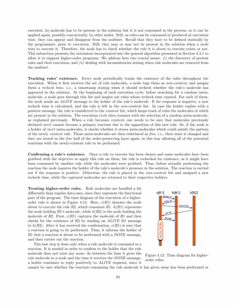
executed, its molecule has to be present in the solution but it is not consumed in the process, so it can beapplied again, possibly concurrently, by other nodes. Still, as rules can be consumed or produced at executiontime, they can appear and disappear from the multiset. Recall that they have to be defined statically bythe programmer, prior to execution. Still, they may or may not be present in the solution when a nodetries to execute it. Therefore, the node has to check whether the rule it is about to execute exists or not.This subsection presents the extensions incorporated into the general algorithm presented in Section 4.3.1 toallow it to support higher-order programs. We address here two crucial issues: (i) the discovery of presentrules and their execution; and (ii) dealing with inconsistencies arising when rule molecules are removed fromthe multiset.
Tracking rules’ existence. Every node periodically tracks the existence of the rules throughout theexecution. When it first receives the set of rule molecules, a node tags them as non-existent, and assignsthem a recheck time, i.e., a timestamp stating when it should recheck whether the rule’s molecule hasappeared in the solution. At the beginning of each execution cycle, before searching for a random meta-molecule, a node goes through this list and singles out rules whose recheck time expired. For each of them,the node sends an ALIVE message to the holder of the rule’s molecule. If the response is negative, a newrecheck time is calculated, and the rule is left in the non-existent list. In case the holder replies with apositive message, the rule is transferred to the existent list, which keeps track of rules the molecules of whichare present in the solution. The execution cycle then resumes with the selection of a random meta-molecule,as explained previously. When a rule becomes existent, one needs to be sure that molecules previouslydeclared inert cannot become a primary reactant due to the apparition of this new rule. So, if the node isa holder of inert meta-molecules, it checks whether it stores meta-molecules which could satisfy the patternof the newly existent rule. Those meta-molecules are then redeclared as free, i.e., their state is changed andthey are stored in the free half of the order-preserving layer again, in this way allowing all of the potentialreactions with the newly-existent rule to be performed.
Confirming a rule’s existence. Once a rule to execute has been chosen and some molecules have beengrabbed with the objective to apply this rule on them, the rule is rechecked for existence, as it might havebeen consumed by another rule while the molecules were grabbed. Thus, before actually performing thereaction the node inquires the holder of the rule’s molecule’s presence in the solution. The reaction is carriedout if the response is positive. Otherwise, the rule is placed in the non-existent list and assigned a newrecheck time, while the captured molecules are returned to their respective holders.
Figure 4.12: Time diagram for higher-order rules.
Treating higher-order rules. Rule molecules are handled a bitdifferently than regular data ones, since they represent the functionalpart of the program. The time diagram of the execution of a higher-order rule is shown in Figure 4.12. Here, c(R1) denotes the nodeabout to execute the rule R2, which consumes R1. h(R1) representsthe node holding R1’s molecule, while h(R2) is the node holding themolecule of R2. First, c(R1) captures the molecule of R1 and thenchecks for the existence of R2 by sending an ALIVE R2 messageto h(R2). After it has received the confirmation, c(R1) is sure thata reaction is going to be performed. Thus, it informs the holder ofR1 that a reaction is about to be performed with a DONE message,and then carries out the reaction.
This last step is done only when a rule molecule is consumed in areaction. It is needed in order to confirm to the holder that the rulemolecule does not exist any more. In between the time it gives therule molecule to a node and the time it receives the DONE message,a holder continues to reply positively to ALIVE requests, since itcannot be sure whether the reaction consuming the rule molecule it has given away has been performed or
61

not; the mere fact of capturing a molecule does not assure a reaction will take place. As we discuss justbelow, this step may introduce inconsistencies during execution. Still, it is mandatory in order to guaranteethe proper detection of inertia.
Potential inconsistencies. As extensively studied in Chapter 3, the chemical programming model en-forces mutual exclusion on molecules — a molecule cannot be used in more than one reaction. Consequently,rule molecules, as others, will not be consumed several times. Still, because the flat reactor is decentralisedand asynchronous, we need to more carefully look at another potential consistency problem: the case wherea rule tries to apply a rule at the same time another node tries to consume its corresponding molecule. Infact, this case can lead to what can be seen as an inconsistency: a node applies a rule after it was consumedby another node. In fact, the protocol lets this happen potentially. We argue that this is not a problem, inthe sense that the chemical model is not naturally armed for such a case: According to the chemical modelexecution model, two active rules at the same depth in the solution can be applied in any order. Again,recall that the only requirement of the model in terms of scheduling is that if at least one rule is active, atleast one reaction is performed. Parallelism, and thus non-determinism is the norm. Let assume a programwith two rules: hr, a higher-order rule consumes the basic rule r. According to the model, if at some pointof the execution, both rules r and hr can be applied, the two possible orders can arise. In fact, once hris active, it can be delayed arbitrarily. Consequently, if r continues to be applied for a while once hr wasapplied, the resulting multiset is amongst the set of valid multisets resulting from the possible executions ofthe program. You can find a more detailed discussion about the inconsistency issue and inertia detectionwhen the higher-order is enabled in the PhD dissertation of Marko Obrovac [77].
4.3.4 Prototype
Figure 4.13: Logical view of the entities formingthe flat reactor prototype.
In order to better capture the performance of the flat re-actor devised, we developed a prototype whose architec-ture is illustrated in Figure 4.13. The logical architectureof the flat reactor prototype is somewhat similar to thatof the hierarchical reactor prototype: The central unitacts as an intermediate module between the applicationand the functional parts (holders and manager describedpreviously), themselves relying on the overlay network fortheir communications. Each entity in the picture commu-nicates with the ones directly above and below it. The ap-plication transfers the program to the central unit, whichthen scatters the molecules and multicasts the rule def-initions via the overlay network. During this period, asfor the hierarchical reactor, the tree manager monitors
the overlay and builds the node’s local state — parent/child relationships with other nodes —, used formulticast requests. More specifically to the flat reactor, the central unit is also in charge of executing themain loop (Algorithm 9). For obtaining random meta-molecules and performing range queries, it consultsthe meta-molecule holder, which communicates with meta-molecule holders on other nodes in order to fulfilthe request. Requests concerning molecules, in particular testing molecules against rules are done by themolecule holder entity. This prototype was developed in Java3.
3The sources are available in the branches/devel-distrib directory of the svn repository located athttp://gforge.inria.fr/scm/?group id=2125.
62

4.3.5 Experimental evaluation
Test programs
The prototype was first tested on two categories of programs. The first one is massively parallel : the sameoperation is applied to data in parallel without synchronization constraints. This category of programsis represented by the getMax program. Recall that the potential of reactions decreases over time duringexecution. Note finally that the number of reactions performed , from one execution to the other, is always thesame, provided the initial number of molecules in the multiset is constant. The second category of programsis producer/consumer programs. This second category exhibit stronger needs in terms of synchronization:once some data has been produced, it is sent over to the consumer. Conversely, the consumer needs to waitfor the producer to emit data to start. It can be seen as a composition of massively parallel sub-programs.This second category was embodied by StringManip — a program comprising two rules manipulating stringmolecules. The logic of StringManip consists in splitting and packing together string molecules in such a waythat the resulting string molecules have a predefined length, denoted λ. The first rule, SplitStr , consumesone molecule whose string’s length is greater than λ and produces two molecules: one composed of the first λcharacters of the original molecule’s string, the other containing its remainder. The second rule, ConcatStr ,takes two molecules as inputs and outputs one which is their concatenation. Thus, SplitStr produces themolecules which are going to be consumed by ConcatStr . The two rules are circularly dependant. Thecourse of the execution of StringManip, as well its outcome, is non-deterministic. While it is known thatat the end of the execution the molecules’ strings are going to have a length of λ, their contents depend onthe succession of reactions performed by the system, which is influenced by the asynchronous nature of theplatform. In other words, the outcome is conditioned by the reactions performed by each node, their inputmolecules, and the order in which they actually take place. Hence, the number of reactions done throughoutthe execution varies from run to run.
To assess the proposed platform’s responsiveness to changes in the program’s set of rules induced by theirdynamic addition and removal, we used a simple program which first calculates the sum of some integers andthen switches its computation to string concatenation based on integers currently present in the solution.The initial solution contains only integer molecules along with the sum rule, which takes two integers andproduces their sum. Then, at a random point in time, a new rule molecule appears — that of switcher , arule erasing sum’s rule molecule — effectively ending the sum epoch. switcher injects two rule molecules:int to str , which turns integers into their string representations; and str concat , which concatenates twostring molecules.
Results
The experiments were also conducted on Grid’50004 [27]. For each run, the nodes were again spread randomlyover the nine geographically-distant sites. Firstly, we evaluated the viability of the platform by executing thefirst two programs while varying the number of nodes participating in the execution. Figures 4.14 and 4.15show the execution times obtained for getmax and StringManip, respectively.
In both cases there is a decrease in execution time when increasing the number of nodes carrying outthe computation. This is to be expected since, the more nodes are active, the more reactions can be donein parallel. This is of course especially true when there is a limited number of conflicts at capture time, thenodes using the optimistic protocol described in Chapter 3. The speed-ups obtained are significant. Still,the speed-up obtained for getmax is greater than that for StringManip. This is due to the difference ofthe programs’ characteristics. The execution time of StringManip depends on the sequentiality of events:certain reactions cannot be carried out before others are. In contrast, the execution of getmax is highlyparallel, as the maximum possible number of reactions can be performed at any given point in time. Also,the execution takes more time to complete for 1000 nodes than for 750 when executing StringManip. Thisis again due to the program’s sequentiality: more nodes are in conflict over a subset of molecules since notall available molecules can be used straight away.
4http://www.grid5000.fr
63

160
180
200
220
240
260
280
300
320
100 200 300 400 500 600 700 800 900 1000
Exe
cu
tio
n t
ime
(s)
Number of nodes
GetMax
Figure 4.14: Execution time of getmax containing50, 000 molecules.
110
120
130
140
150
160
170
180
190
100 200 300 400 500 600 700 800 900 1000
Exe
cu
tio
n t
ime
(s)
Number of nodes
StringManip
Figure 4.15: Execution time of StringManip with20, 000 molecules.
During the previous experiments, we also monitored the network traffic generated. Our findings con-cerning the number of messages is that it increases linearly with the number of nodes (for both programs,with a constant number of molecules). Still, the number of messages per nodes decline with the growth ofthe network, which shows the scalability of the platform on the network side. Finally, we conducted someexperiments varying the initial number of molecules while keeping the number of nodes constant (using thegetmax program). These experiments show that both the execution time and number of messages also in-crease linearly with the number of molecules. Again, the average number of messages per reaction decreasewith the number of molecules. This is due to the fact that there are less conflicts, confirming experimen-tally the relevance of the adaptive capture protocol, and reinforcing the evidences of the scalability of theplatform. The details of these results can be found in [78].
The second part of our experimental campaign dealt with the evaluation of the higher order, under twodimensions: the overhead it brings about to the execution, and its responsiveness, i.e., its quickness toactually stop applying a rule whose molecule has been consumed. About the first dimension, our experi-mental findings are that the rule-check procedure introduces an overhead which increases with the numberof molecules, as it is repeated each time the application of a rule is attempted. Still, the general behaviourof both the execution time and generated network traffic remains linear in the size of the problem.
0
5
10
15
20
25
30
0-0.5 0.5-1 1-1.5 1.5-2 2-2.5 2.5-3 3-3.5
Nu
mb
er
of
run
s
Time intervals (s)
Figure 4.16: Responsiveness of the platform withregards to the time it takes to detect the disappear-ance of a rule.
0
5
10
15
20
25
30
0-5 5-10 10-15 15-20 20-25 25-30 30-35
Nu
mb
er
of
run
s
Intervals of number of reactions (x10)
Figure 4.17: Responsiveness of the platform interms of number of reactions done with a non-existing rule.
Our last experiment, whose results are represented in Figures 4.16 and 4.17, we used the higher-orderprogram described above in order to assess the platform’s responsiveness to dynamic changes in the program’sexecution flow. We executed the program 100 times on a network of 250 nodes, changing the network
64

configuration each time by randomly choosing the site, the cluster and the port number of each node. Wemeasured the time it took to all of the nodes to detect that the sum rule’s molecule is not present in thesolution any more. At the beginning of each run all of the nodes’ internal clocks were synchronised in orderto obtain precise measurements. Figure 4.16 shows the number of runs in which the nodes stopped executingthe rule after its disappearance from the solution, divided in half-second intervals. Likewise, Figure 4.17shows the number of reactions carried out during that period.
As explained in Section 4.3.3, this delay manifests itself because sum’s molecule’s holder replies positivelyto rule check requests until it has received the confirmation of its consumption. This delay depends on theunderlying network’s delay. Based on Figure 4.16, we observe that in 81% of runs, nodes stop executing therule at most two seconds after its disappearance, while the highest delay is 3.5 seconds, observed in only 3%of runs. Even though this might seem as a long period of time, the two-second delay represents only 1% ofthe overall execution time. In the same vein, Figure 4.17 suggests that in 79% of runs, nodes do at most 200reactions during the delay, which represents 1% of the total number of reactions done during the executionand less than one reaction per node.
4.4 Conclusion
This chapter discussed our works around the design, development and experimental validation of two dis-tributed runtime systems for chemical programs. The first, hierarchical reactor is conceptually simple andbuilds an execution tree in which the inert sub-solutions are fused until reaching the root of the tree. Thehierarchical reactor does not need complex algorithmic, just a bit of care when parent nodes receive inertsub-solutions from their children, to avoid losing the work achieved in their subtree. The hierarchical re-actor suffers from its shape, potentially leading to great disparities in terms of workload across nodes. Itis also hard to extend to support higher-order programs. In contrast, the flat reactor is fully decentralisedand does not include any by-design non-uniform load balancing. It includes a molecule discovery protocolbased on a two-layer DHT and complex queries allowing to detect early that some molecules may not reactanymore. This pruning scheme was not fully exploited in our work, as anyway all molecules are scannedat least once by some node. Extending such a complex querying-based inertia detection could allow tosignificantly reduce execution time when a lot of molecules cannot react anymore. Due to the full decentral-isation and the subsequent need for a molecule discovery mechanism, a capture protocol is needed to avoidseveral nodes discovering overlapping sets of molecules to allocate them at the same time. The flat reactorleverages the adaptive capture protocol of Chapter 3 to address this issue. Finally, the flat reactor supportsthe higher-order.
Both reactors have been implemented, deployed and evaluated over a geographically dispersed platform.To our knowledge, these works were the first to distribute the execution of chemical programs at such ascale, giving hints for the potential usage of the paradigm over massively distributed platforms.
This chapter closes the part of this dissertation dedicated to the model itself and its implementation indistributed settings. Now that some barriers towards its practical usage have been lifted, it is time to seein more detail how the programming model it offers can be used to help programming autonomic systems,and more specifically how it can be used to specify service composition and workflows with adaptivenesscapabilities.
65


Chapter 5
Decentralising Workflow Execution
Previous chapters dealt with the chemical programming model and its implementation in distributed settings.The two following chapters are more about how it can be used to program (workflow-based) applications andhelp bring decentralisation and adaptiveness to their execution. This chapter deals with the decentralisationof workflow execution. It shows how a set of agents can coordinate themselves to share the coordination of theexecution. To this end, we devise a shared-space architecture on top of which chemically-inspired abstractionsare used to express the workflow and its enactment. The implementation of these concepts into the GinFlowmiddleware is detailed and their experimental validation discussed.
Joint work with:
? Hector Fernandez (PhD student, Inria)? Thierry Priol (Senior researcher, Inria)? Matthieu Simonin (Research engineer, Inria)
5.1 Workflows, workflow managers, and decentralisation
As we have discussed more extensively in Introduction, service composition is an attractive paradigm to buildcomplex applications out of more basic yet well-defined basic services. Service compositions (or compositeservices are most commonly temporal composition of such building block services. Industrial organizationsuch as the OASIS consortium proposed many standards to help program and manage service-orientedarchitectures. Architectures following these standards (most of them following an XML-based grammar)have been notoriously known as web services, a term that is now commonly used to describe any flavour ofweb-based application, would it be built over SOAP or using a RESTful approach. BPEL (Business ProcessExecution Language) is one of these standards, specifically targeted at describing service composition. Itcan be seen as the assembly language for service composition, embedding a lot of implementation details(protocols used, service locations, . . . ) and being globally very verbose. The abstraction level provided byBPEL does not allow the programmer to concentrate on the logic of the composition properly.
This lack of a high-level programming model for service composition is in particular a barrier in thescientific world. In many scientific domains, simulation experiments is now the dominant paradigm forresearch. These compute-intensive simulations commonly compose functional building blocks together. Suchcompositions are referred to as (scientific) workflows. The concept of workflow is very similar to servicecomposition. More formally, a workflow can be represented by a graph in which each vertex is a function,or service and each edge a data dependency or a control dependency between services. Workflows are nowwidely used, reused and shared among scientific communities, as for instance through the myExperiment1
workflow sharing platform.
1http://www.myexperiment.org
67
Workflow management systems such as Taverna [103], Kepler [69] and MOTEUR [53] have focused onproviding tools to design and execute scientific workflows with a high level of abstraction. These workflowmanagers all rely at some point on a centralised orchestrator responsible for coordinating the workflowexecution. The drawbacks of such an element have been discussed in Introduction. While limited, someworkflow research focused on enabling direct cooperation between services in order to allow executions evenin the case no central engine is available. We will come back to these works later in the chapter, for thesake of comparing our proposal with the state of the art. Getting rid of a centralised manager and allowsfor horizontal scalability, and raises the level of reliability and even privacy. It globally moves the systemtowards more autonomy. Please refer back to Chapter for this discussion.
In Section 5.2, we present first an architecture aiming at enacting workflows in a decentralised fashion.This architecture relies on a shared space for coordination between services involved in the workflow. We thenpresent in Section 5.3, based on this architecture, a programmatic way to specify workflows over decentralisedsettings. The implementation of these concepts was done through the development of a research prototypeduring Hector Fernandez’ PhD [44]. This software prototype was later turned into the more mature GinFlowworkflow manager2 presented in Section 5.4. In particular, GinFlow’s software architecture and resiliencemechanisms are detailed. GinFlow’s scalability and resilience, and thus the viability of these conceptsare validated through a set of experiments conducted over the Grid’5000 platform in Section 5.5. Beforeconcluding the chapter, Section 5.6 positions this work in the landscape of distributed workflow coordinationresearch.
5.2 Shared-space based coordination
The execution model we have proposed is to enact a decentralised execution through the splitting of thetraditional workflow engine (or composition orchestrator) into a set of agents co-responsible for the executionof the workflows. The architecture includes two types of components, namely i) the shared space whichcontains the description of the workflow and ii) the service agents (SAs) which will share the coordinationwork in executing the workflow described in the shared space. During enactment, each time the executionmoves forward after some action performed by some agent, the shared description is updated so as to reflectthe execution progress. The SAs are essentially workers that encapsulate the invocation of the services. Thisencapsulation includes an engine able to read, interpret and update the information contained in the sharedspace. For instance, when a SA completes the invocation of a service and collects the result, it pushes thisinformation to the shared space, allowing another service agent, which was waiting for this result, to collectit and use it as input to invoke the service it encapsulates.
A possible scenario of execution in such an architecture is depicted in Figure 5.1: i) the shared space(represented as a circle surrounding the graph) is fed with the description of the workflow and each SAcollects from it the information it needs to actually takes its part in the coordination (incoming and outgoingdependencies, and services to call); ii) The SA checks the information received and the ones that can startdoing something (i.e., those responsible for services with no incoming dependencies) actually trigger theexecution of the workflow; iii) Once a SA completes the execution of its services, it sends its output to itsdependencies and updates the shared space so as to reflect that the workflow moves forward which make thesubsequent parts of the workflow able to start in their turn; iv-v-vi) this process is repeated until the wholeexecution is completed.
The relation between such an architecture and HOCL is kind of straightforward: replace shared spaceby multiset and Service Agents by HOCL engines applying HOCL rules on part of this multiset and youare done. Also, having a declarative programming style helps to easily express the coordination. To sumup, in the context of this decentralised workflow executor, the initial multiset will contain the descriptionof the workflow, and the rules will express how to modify this description so as to reflect the execution is
2https://ginflow.inria.fr
68

SA
SA
SA
SA
i)
SA
SA
SA
SA
ii)
SA
SA
SA
SA
iii)
SA
SA
SA
SA
iv)
SA
SA
SA
SA
v)
SA
SA
SA
SA
vi)
Figure 5.1: An example of shared-space coordination.
moving forward. As we will see in details, the needs are simple: i) expressing that a service is called (onceall its dependencies have been satisfied) and ii) expressing that data are moved once a service’s call has beencompleted.
5.3 Chemical workflow specification
We now use an extended version of HOCL named HOCLflow. It is introduced specifically for workflowexpression. HOCLflow provides extra syntactic facilities over HOCL. Firstly, it includes lists (which are notnatively supported by HOCL). Secondly, it offers some syntactic sugar avoiding to double mention catalystsin reaction rules. More precisely, rules of the form: replace-one X by X, M where X and M are multisetsof molecules, can be written: with X inject M . Thirdly, it includes reserved keywords for specific atomsto ease the workflow management. They will be explained when used hereafter.
A workflow is mostly a set of tasks to be executed in a certain order. A task can be seen as an abstractfunction, to be implemented by a service. A workflow can be represented as a directed acyclic graph (DAG),as illustrated in Figure 5.2.
An HOCL workflow definition is composed of as many subsolutions as there are tasks in the workflow.The HOCL code for the workflow in Figure 5.2 is given in Figure 5.3. Each subsolution is similar andcontains (initially) four atoms. The first two tuple atoms, prefixed by the reserved keywords src and dst,specifies the incoming and outgoing dependencies of the task, respectively. The two latter atoms provide thedata needed to invoke the service, namely, its name (in the srv atom) and its parameters (in the in atom).Recall that src, dst, srv and in are reserved keywords in HOCLflow.
Still, if the code in Figure 5.3 is given as input to an HOCL interpreter, it will not trigger anything—itdoes not comprise rules. Thus, we need to design a set of rules able to, when combined with a workflowdescription, execute the specified workflow. We now devise a set of three simple rules which constitutes theminimal set of rules allowing any workflow to run. We call these rules generic and prefix their name with
69
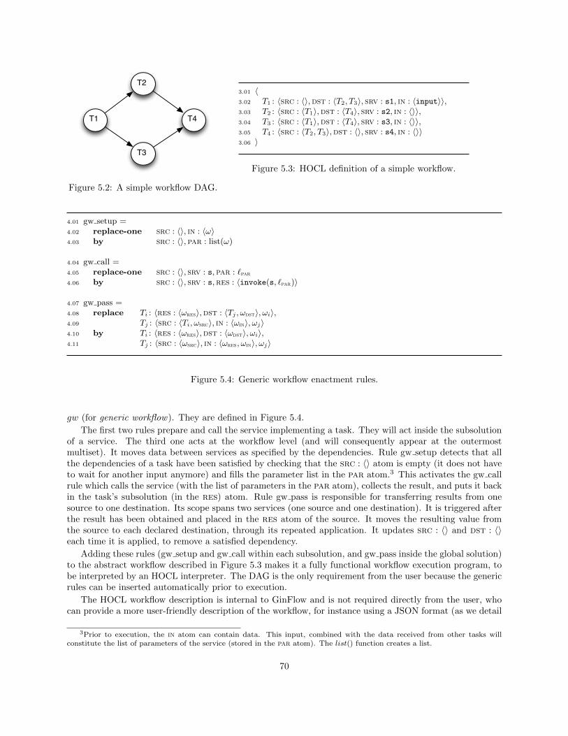
T1
T2
T3
T4
Figure 5.2: A simple workflow DAG.
3.01 〈3.02 T1 : 〈src : 〈〉,dst : 〈T2, T3〉, srv : s1, in : 〈input〉〉,3.03 T2 : 〈src : 〈T1〉,dst : 〈T4〉, srv : s2, in : 〈〉〉,3.04 T3 : 〈src : 〈T1〉,dst : 〈T4〉, srv : s3, in : 〈〉〉,3.05 T4 : 〈src : 〈T2, T3〉,dst : 〈〉, srv : s4, in : 〈〉〉3.06 〉
Figure 5.3: HOCL definition of a simple workflow.
4.01 gw setup =4.02 replace-one src : 〈〉, in : 〈ω〉4.03 by src : 〈〉, par : list(ω)
4.04 gw call =4.05 replace-one src : 〈〉, srv : s, par : `par4.06 by src : 〈〉, srv : s,res : 〈invoke(s, `par)〉
4.07 gw pass =4.08 replace Ti : 〈res : 〈ωres〉,dst : 〈Tj , ωdst〉, ωi〉,4.09 Tj : 〈src : 〈Ti, ωsrc〉, in : 〈ωin〉, ωj〉4.10 by Ti : 〈res : 〈ωres〉,dst : 〈ωdst〉, ωi〉,4.11 Tj : 〈src : 〈ωsrc〉, in : 〈ωres, ωin〉, ωj〉
Figure 5.4: Generic workflow enactment rules.
gw (for generic workflow). They are defined in Figure 5.4.
The first two rules prepare and call the service implementing a task. They will act inside the subsolutionof a service. The third one acts at the workflow level (and will consequently appear at the outermostmultiset). It moves data between services as specified by the dependencies. Rule gw setup detects that allthe dependencies of a task have been satisfied by checking that the src : 〈〉 atom is empty (it does not haveto wait for another input anymore) and fills the parameter list in the par atom.3 This activates the gw callrule which calls the service (with the list of parameters in the par atom), collects the result, and puts it backin the task’s subsolution (in the res) atom. Rule gw pass is responsible for transferring results from onesource to one destination. Its scope spans two services (one source and one destination). It is triggered afterthe result has been obtained and placed in the res atom of the source. It moves the resulting value fromthe source to each declared destination, through its repeated application. It updates src : 〈〉 and dst : 〈〉each time it is applied, to remove a satisfied dependency.
Adding these rules (gw setup and gw call within each subsolution, and gw pass inside the global solution)to the abstract workflow described in Figure 5.3 makes it a fully functional workflow execution program, tobe interpreted by an HOCL interpreter. The DAG is the only requirement from the user because the genericrules can be inserted automatically prior to execution.
The HOCL workflow description is internal to GinFlow and is not required directly from the user, whocan provide a more user-friendly description of the workflow, for instance using a JSON format (as we detail
3Prior to execution, the in atom can contain data. This input, combined with the data received from other tasks willconstitute the list of parameters of the service (stored in the par atom). The list() function creates a list.
70

later in Section 5.4). This JSON definition will be then translated internally so as to obtain the requiredHOCL representation.
5.01 〈5.02 T1 : 〈src : 〈〉,dst : 〈T2, T3〉, srv : s1, in : 〈input〉〉,5.03 T2 : 〈src : 〈T1〉,dst : 〈T4〉, srv : s2, in : 〈〉〉,5.04 T3 : 〈src : 〈T1〉,dst : 〈T4〉, srv : s3, in : 〈〉〉,5.05 T4 : 〈src : 〈T2, T3〉,dst : 〈〉, srv : s4, in : 〈〉〉5.06 〉
i.
6.01 〈6.02 T1 : 〈src : 〈〉,dst : 〈T2, T3〉, srv : s1,res : 〈r1〉〉,6.03 T2 : 〈src : 〈T1〉,dst : 〈T4〉, srv : s2, in : 〈〉〉,6.04 T3 : 〈src : 〈T1〉,dst : 〈T4〉, srv : s3, in : 〈〉〉,6.05 T4 : 〈src : 〈T2, T3〉,dst : 〈〉, srv : s4, in : 〈〉〉6.06 〉
ii.
7.01 〈7.02 T1 : 〈src : 〈〉,dst : 〈〉, srv : s1,res : 〈r1〉〉,7.03 T2 : 〈src : 〈〉,dst : 〈T4〉, srv : s2, in : 〈r1〉〉,7.04 T3 : 〈src : 〈〉,dst : 〈T4〉, srv : s3, in : 〈r1〉〉,7.05 T4 : 〈src : 〈T2, T3〉,dst : 〈〉, srv : s4, in : 〈〉〉7.06 〉
iii.
8.01 〈8.02 T1 : 〈src : 〈〉,dst : 〈〉, srv : s1,res : 〈r1〉〉,8.03 T2 : 〈src : 〈〉,dst : 〈T4〉, srv : s2,res : 〈r2〉〉,8.04 T3 : 〈src : 〈〉,dst : 〈T4〉, srv : s3,res : 〈r3〉〉,8.05 T4 : 〈src : 〈T2, T3〉,dst : 〈〉, srv : s4, in : 〈〉〉8.06 〉
iv.
9.01 〈9.02 T1 : 〈src : 〈〉,dst : 〈〉, srv : s1,res : 〈r1〉〉,9.03 T2 : 〈src : 〈〉,dst : 〈〉, srv : s2,res : 〈r2〉〉,9.04 T3 : 〈src : 〈〉,dst : 〈〉, srv : s3,res : 〈r3〉〉,9.05 T4 : 〈src : 〈〉,dst : 〈〉, srv : s4, in : 〈r3, r2〉〉9.06 〉
v.
10.01〈10.02 T1 : 〈src : 〈〉,dst : 〈〉, srv : s1,res : 〈r1〉〉,10.03 T2 : 〈src : 〈〉,dst : 〈〉, srv : s2,res : 〈r2〉〉,10.04 T3 : 〈src : 〈〉,dst : 〈〉, srv : s3,res : 〈r3〉〉,10.05 T4 : 〈src : 〈〉,dst : 〈〉, srv : s4,res : 〈r4〉〉10.06〉
vi.
Figure 5.5: Simple workflow’s execution scenario.
The evolution of the multiset during execution is illustrated in Figure 5.5. Between state i. and stateii., the agent responsible for T1 applied both gw setup and gw call and the result of s1 appears in a newlycreated res : 〈〉 atom. Then, to reach State iii., the gw pass rule was applied twice, once for each neededtransfer towards T2 and T3’s subsolutions. Then, in parallel, respective service agents responsible for T2 andT3 was able to gw setup and gw call in their turn so as to create their respective results r2 and r3. Towardsstate v., and still in parallel, the same SAs apply gw pass so as to move their results to T4. The arrival orderof results into T4’s subsolution is not predetermined. The multiset reaches its final state (vi.) with the SAresponsible for T4 executing s4 and getting its outcome.
5.4 GinFlow
This section presents the GinFlow workflow middleware. It is the result of a significant refactoring andextension of the early prototype developed by Hector Fernandez and presented in [46]. It was made a moremature, usable and extensible software by Matthieu Simonin, research engineer at Inria. Its code was releasedunder the LGPL-3 license in 2016. It is registered at the APP (Agence de Protection des Programmes) underthe number IDDN.FR.001.46018.000.S.P.2015.000.10600.4
GinFlow sits on the HOCL language and interpreter which consists in 18 000 lines of Java code developedby Yann Radenac, during his PhD defended in 2007 [83]. The middleware itself represents approximately
4To download and try it, please go to https://ginflow.inria.fr.
71

2 000 more lines of Java code. Figure 5.6 depicts the general GinFlow architecture. This architecture ismade of three layers. In Section 5.4.1, we present the bottom layer of the architecture and highlights theinternals of the core engine. In Section 5.4.2, the resilience of this layer is described. Section 5.4.3 focuseson the intermediate level of the architecture, the executor layer in use in GinFlow. Section 5.4.4 deals withthe upper level providing ways to users to interact with GinFlow.
5.4.1 The HOCL distributed engine
At the core (the lower layer in Figure 5.6), the GinFow middleware consists in a distributed engine, whichimplements the concepts of service agents (SAs) communicating through a shared space containing thedescription of the current status of the workflow. In GinFlow, a SA is composed of three elements. The firstelement is the service to invoke, any wrapper of an application representing this service, or any interface tothe service enabling its invocation. The second element is a storage place for a local copy of the multiset.The local copy acts as a cache of the service’s subsolution. The third element is an HOCL interpreter thatreads and updates the local copy of the multiset each time it tries to apply one of the rule in the subsolution.A SA stores locally only the status of the portion of the workflow it is responsible for. The cache is only readand written locally by this single interpreter, and often pushed back (written) to the shared space, ensuringno coherency problems can arise.
Once each SA collected data from the multiset, it communicates directly with other agents in a point-to-point fashion, for instance when transmitting data between two workflow tasks. Recall that, as earlierdescribed in Section 5.3, enactment rules have to be injected into the workflow description prior to itsexecution, (i.e., before any agent starts collecting its initial information from the multiset).
More precisely, the rules presented in Section 5.3 do not enable a decentralised execution by themselves.In particular, looking carefully at the gw pass rule, whose detailed functioning was until now eluded, we cansee it spans several subsolutions and it is thus supposed to act from outside subsolutions since it requires tomatch the atoms from several subsolutions. In the GinFlow environment, it was modified to act from within
Local
Command Line Interface
GINFLOW API (JAVA)
JSON Code
EXECUTOR
Centralized Distributed
SSH MESOS EC2*
result
result
HOCL workflowHOCL
interpreter
S
Local multiset
start
result
MQ
Figure 5.6: Architecture of the GinFlow software.
72

a subsolution: once the result of the invocation of the service it manages is collected, a SA triggers a localversion of the gw pass rule which calls a function that sends a message directly to the destination SA. It alsosends a message to the multiset so as to update the status of the workflow. When the message is received inthe multiset, it is simply pushed to the right subsolution.
In GinFlow, the inter-agents communications rely on a message queue middleware which can be eitherApache ActiveMQ or Apache Kafka. The choice for one or the other depends on the level of resilience neededby the user, as we detail below.
5.4.2 Resilience
In this section, we present a mechanism that automates the recovery of failed server agents. When one SAfails, for instance following a hardware crash, another SA will be automatically started to replace it. Thedifficulty here stands in the ability to replay the work done by the faulty SA prior to its failure.
The state of a SA is reflected by the state of its local solution. Changes in the local solution can resultfrom two mutually exclusive actions : i) reception of new molecules and ii) reduction of the local solutionthrough the action of the local HOCL engine it embeds. A reduction phase is systematically triggered whennew molecules are received. Note that this reduction modifies the state of the local solution only if somerule were actually applied during reduction. The SA lifecyle is thus a sequence of receptions and reductions.Consequently, if the system is able to keep the information of all molecules received by a SA and resendthem in the same order to a newly created SA, this second SA can recover the state of the first one.
This soft-state behaviour of the SAs let us envision a fault-recovery mechanism which will rebuild thestate of a faulty SA. It is assumed that the actual services invoked are idempotent, or at least free from non-desirable side effects since they can be called several times in case the fault-recovery mechanism is triggered.Still, some results may be received several times by some of the successor nodes of a recovered SA, in casethe first SA failed after invoking the service but before finishing the transmission of its results to all of itssuccessors. However, the one-shot nature of the gw setup and gw call rules ensures that the successors willtake into account only the first result received and thus prevent a cascade of useless re-executions.
In GinFlow’s implementation, this resilience feature leverages Kafka’s ability to persist the messagesexchanged by the SAs and to replay them on demand to facilitate the implementation of this mechanism.Section 5.5.3 will present an evaluation of GinFlow’s resilience.
5.4.3 The executors
The role of the executor is to prepare, deploy the distributed engine, and bootstrap the workflow in a specificenvironment, either centralised or distributed. The centralised executor relies on a single HOCL interpreterto execute the workflow. A distributed executor will (1) claim resources from the infrastructure and (2)provision the distributed engine (the SAs and the multiset) on them. The deployment is made of threephases to be described hereafter: preparation, deployment, and bootstrapping phases.
Preparation phase. Users only deal with abstract workflows, i.e., specify the workflow itself withoutneeding to deal with enactment considerations. In other words, the user provides some description, usingthe GinFlow API to be described in Section 5.4.4, that will be translated into its HOCL equivalent code,as illustrated in Figure 5.2. To allow the enactment of the workflow, rules need to be injected to producea concrete workflow description. This consists in adding the gw setup, gw call, and gw pass rules intothe HOCL workflow representation. This injection occurs during the preparation phase and is performedtransparently for the user.
Deployment phase. In the current version of GinFlow, two distributed executors are available: SSH-based and Mesos-based. The SSH-based executor starts the SAs on a set of machines specified by the user inthe GinFlow configuration file. It deploys the SAs over the machines in a round-robin fashion. The Mesos-based executor delegates the deployment of the SAs to the Mesos scheduler [56]. Besides these executors,
73

the abstract nature of the code allows GinFlow to be easily extended with other executors (such as an EC2executor to run GinFlow’s distributed engine on an EC2-compatible cloud).
Bootstraping phase. Once the SAs are deployed over the computing nodes, the workflow execution isstarted by sending its initial description (including the injected rules) to the SAs. These communicationsrely on the same communication layer as the execution: ActiveMQ or Kafka, as configured by the user.Upon reception, each SA will start reducing its own solution and thus executing the workflow.
5.4.4 Client interfaces
We here describe how the user interacts with GinFlow. The user is given two entry points: GinFlow’scommand line and GinFlow’s Java API. The former consists in defining the workflow in a JSON-formattedfile with the specification of all the tasks and the links between them. The latter uses the internal JavaAPI of GinFlow to describe the DAG programmatically. We again use the workflow depicted in Figure 5.2for the sake of illustration. Assuming the JSON file describing the workflow was saved under the namewf-1.json, the command line below starts the workflow using the centralised executor, i.e., using only oneHOCL interpreter running in the same JVM as the main program:
java -jar hocl-workflow-2.0.0-SNAPSHOT.jar launch -w wf-1.json
To distribute the execution over different processes but still on the same physical computing node, onecan specify an alternate executor on the command line. For instance, adding -e ssh to the command linedistributes the execution using the SSH protocol. Without any further configuration except a passwordlessSSH connection, this will result in distributing three service agents, each one running an HOCL interpreterlocally and communicating through an embedded version of ActiveMQ, the by default broker started by theGinFlow executor prior to workflow execution. To distribute the SA processes over different machines, orto rely upon one’s specfific broker, the user can specify a set of options either through the -o switch in thecommand line, or by using a configuration file following the YAML format.
For more advanced usages, GinFlow exposes a Java API. This programming interface gives the program-mer the possibility to define easily higher-level workflow patterns (e.g., a sequence of tasks) and to configurethe options of the executor and even start the exection, for instance to start GinFlow from another Javaprogram. Listing 1 exposes the Java definition of the workflow.
5.5 Experimental validation
In this section, we present the results of the experimental evaluation of GinFlow. The results exhibited in thefollowing revolves around i) performance and scalability, ii) the impact of choosing different combinations ofexecutors and messaging middleware, and iii) the SA recovery mechanism presented in Section 5.4.2. Notethat we considered only distributed settings, as it constitutes the natural playground of GinFlow and ourmotivation for this work.
Experimental setup. All the experiments were run using up to 50 multi-core computing nodes of theGrid’5000 testbed, connected through 1Gbps Ethernet. Debian/Linux Wheezy was installed on the nodesand we used ActiveMQ 5.6.0 and Kafka 0.8.1.1 as the communication middleware. Mesos 0.20 was alsoinstalled on the nodes. A total of 800 cores and 6 TB RAM were used. In the deployments, the number ofSAs per core was limited to two, which allowed to deploy up to 2 603 services.
Workflow shapes. Possible shapes of workflows are virtually infinite, however four major patterns, namelysplit, merge, sequence and parallel have been recognised to cover the basic needs of scientific computationalpipelines [84]. We consequently decided to conduct the experiments of Sections 5.5.1 and 5.5.2 using adiamond shape, depicted in Figure 5.7 and covering the four aforementioned patterns. The shape of diamondworkflow varies according to two parameters: h (for horizontal), the number of services in parallel at each
74
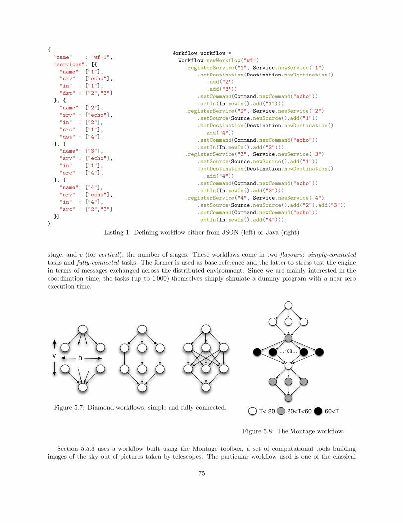
{
"name" : "wf-1",
"services": [{
"name": ["1"],
"srv" : ["echo"],
"in" : ["1"],
"dst" : ["2","3"]
}, {
"name": ["2"],
"srv" : ["echo"],
"in" : ["2"],
"src" : ["1"],
"dst" : ["4"]
}, {
"name": ["3"],
"srv" : ["echo"],
"in" : ["1"],
"src" : ["4"],
}, {
"name": ["4"],
"srv" : ["echo"],
"in" : ["4"],
"src" : ["2","3"]
}]
}
Workflow workflow =
Workflow.newWorkflow("wf")
.registerService("1", Service.newService("1")
.setDestination(Destination.newDestination()
.add("2")
.add("3"))
.setCommand(Command.newCommand("echo"))
.setIn(In.newIn().add("1")))
.registerService("2", Service.newService("2")
.setSource(Source.newSource().add("1"))
.setDestination(Destination.newDestination()
.add("4"))
.setCommand(Command.newCommand("echo"))
.setIn(In.newIn().add("2")))
.registerService("3", Service.newService("3")
.setSource(Source.newSource().add("1"))
.setDestination(Destination.newDestination()
.add("4"))
.setCommand(Command.newCommand("echo"))
.setIn(In.newIn().add("3")))
.registerService("4", Service.newService("4")
.setSource(Source.newSource().add("2").add("3"))
.setCommand(Command.newCommand("echo"))
.setIn(In.newIn().add("4")));
Listing 1: Defining workflow either from JSON (left) or Java (right)
stage, and v (for vertical), the number of stages. These workflows come in two flavours: simply-connectedtasks and fully-connected tasks. The former is used as base reference and the latter to stress test the enginein terms of messages exchanged across the distributed environment. Since we are mainly interested in thecoordination time, the tasks (up to 1 000) themselves simply simulate a dummy program with a near-zeroexecution time.
hv
Figure 5.7: Diamond workflows, simple and fully connected.
…108…
T< 20 20<T<60 60<T
Figure 5.8: The Montage workflow.
Section 5.5.3 uses a workflow built using the Montage toolbox, a set of computational tools buildingimages of the sky out of pictures taken by telescopes. The particular workflow used is one of the classical
75

Montage workflows. It outputs a 3-degree centered image of the M45 star cluster (often referred to as thepleiades) composed of 100 million pixels. It is depicted in Figure 5.8 with the category of duration, inseconds, of its 118 tasks.
5.5.1 Performance
Figure 5.9 shows the timespan for both diamond configurations. It has been obtained by measuring theexecution time for all diamond shapes where width × height ∈ [1, 51]2 with a step of 5 on each dimension.We observe a sustained time increase when the number of services grows. In a simply-connected configuration,the coordination time of the whole workflow execution is close to 155 seconds for 51× 51 services. This timeincludes the exchange information between linked services and the update of the shared multiset. Theseresults are expected because the number of tasks has a direct influence on the time needed for the reductionof sub-solutions: in an HOCL engine, the complexity of the pattern matching process depends on the sizeof the solution. However, the load of evaluating molecules in the global solution is distributed among allco-engines preventing a combinatorial explosion. The same behaviour is observed with the fully-connectedconfiguration. In this case, we observe the higher cost of coordination and the impact of connections betweenservices. Since a service has to wait for all services of the previous layer, an implicit coordination barrier isset in each service growing the final execution timespan (up to 530 seconds for 51 × 51 services). We canalso identify this effect on the projection of the vertical services on the time-vertical plane which shows ahigher slope than the time-horizontal one. While a chemical engine has a potential performance bottleneckfor a large set of services, increasing the number of co-engines limits the final coordination time due to theparallelism, ensuring the scalability of GinFlow in distributed settings.
width10
2030
4050
length10
2030
4050
tim
e (
s)
20
40
60
80
100
120
140
width10
2030
4050
length10
2030
4050
tim
e (
s)
100
200
300
400
500
Figure 5.9: Coordination time of diamond workflows, simple-connected (left) and fully-connected (right).
5.5.2 Impact of the executor and messaging middleware
Figure 5.10 depicts the average time (computed over ten runs) to execute of a 10× 10 diamond workflow ineach executor/communication middleware combination for different number of nodes. It shows the durationof each step: (a) the deployment time (the time taken by the executor to deploy the SAs) and (b) theexecution time. Note firstly that the deployment time depends on the scheduling strategy used. The SSH-based executor starts SAs in a round-robin fashion on a preconfigured list of nodes. As the SSH connectionsare parallelized, the deployment time only slightly increases with the number of nodes. GinFlow, when runon top of Mesos, starts one SA per machine for each offer received from the Mesos scheduler. Thus, increasingthe number of nodes will increase the number of machines in each offer and consequently the parallelization
76

in starting the SAs. This explains the linear decrease of the deployment time observed for the Mesos-basedexecutor.
5 10 15 5 10 15 5 10 15 5 10 15Nodes
0
20
40
60
80
100
Tim
e (
s)
SSH/ActiveMQ
SSH/Kafka
Mesos/ActiveMQ
Mesos/Kafka
10x10 Diamond Simple Connected
ExecutionDeployment
Figure 5.10: Execution time vs configurations.
About the impact of the messaging middleware,ActiveMQ outperforms Kafka as the execution time isapproximately 4 times higher with the latter. Never-theless, the choice of deploying GinFlow with Kafka isjustified by the resilience it helps to provide, as it isexperimented in the next section.
5.5.3 Resilience
We finally evaluated the resilience mechanisms ex-posed in Section 5.4.2. These experiments were basedon the Montage workflow whose shape and durationof tasks are given in Figure 5.8, and made use of theMesos-based executor (to restart agents) and Kafkaas the communication middleware (to persist and re-play messages). Note that the services taken from theMontage toolbox are idempotent, in the sense that aservice can get restarted safely in the case of a failedprevious attempt of executing this service (in the same workflow). The methodology for injecting failureswas the following: each running agent failed with a predefined probability p, but never before a certainamount of time T elapsed since they started executing their task. Note that a restarted agent can fail again.Thus, we can expect p
1−p ×NT (5.1) failures where NT is the number of services whose duration is greaterthan T .
For each chosen value of p and T , we repeated the execution of the workflow up to 10 times and averagedtheir resulting values. The bar plots of Figure 5.11 show the execution time with different values for p andT . The dashed line common to every subplot corresponds to the execution time without any failure. In thiscase the execution time is 484s in average with a standard deviation of 13.5 seconds.
Firstly, when T = 0, increasing p allows to appreciate the recovery velocity. We observed 26, 114 and 487failures in average for p = 0.2, p = 0.5 and p = 0.8 respectively. These observations conform to the resultsobtained with Formula 5.1 with N0 = 118. Figure 5.11 shows an increase of 3s, 36s and 208s respectivelyin the average execution time of the workflow, showing that the recovery velocity slightly decreases whenincreasing the failures rate. In other words, the ratio between the overhead and the number of failuresslightly increases.
Secondly, choosing T = 15s experimentally confirms that services can recover even if they fail after someprocessing. Moreover, note that 95% of the services of this workflow have a running time greater than 15sand thus may be affected by failures. Still, the durations of the services in the large parallel part of theworkflow are quite heterogeneous: from 60s, and up to 310s. Consequently, some services in this part canrecover without impacting the global execution time, as their total execution time will still be under theexecution time of that of other services running free of failure. In contrast, the execution time of the workflowis more sensitive to the failures of some specific services such as the intermediate merging ones. These twoconsiderations can explain the increase of the standard deviation observed in Figure 5.11.
Finally, choosing T = 100s impacts exclusively services in the large parallel part of the workflow. Whilethe observed increase in the execution time necessarily becomes more important (but still in accordance withFormula 5.1, it illustrates the ability of GinFlow to enact real-world workflows reliably over very unstableinfrastructures.
5.6 Decentralising workflow execution in literature
The idea of describing direct interactions between services in the execution of a composition was proposed inthe concept of choreography of web services [13]. Choreography allows to describe at once all the interactions
77

0.2 0.5 0.8p
0
500
1000
1500
2000
2500
3000
Execu
tion t
ime (
s)
T=0s
0.2 0.5 0.8
T=15s
0.2 0.5 0.8
T=100s
Figure 5.11: Execution time with different failure scenarios.
that will take place at execution time. It allows to be more precise than orchestration in which the executionis seen from a single point of view. As detailed in [44], the choreography models proposed in literature isquite static and increase the tight coupling between participants. Also, the concept remained quite abstractover the years. Finally, note that adapting a choreography is difficult issue, subject to be tackled, but notin the context of choreography but in the context of GinFlow, in the next chapter.
Decentralising the coordination of the workflow execution was first pursued relying on direct interactions(based on messaging) between services. In [21], the authors introduce service invocation triggers, a lightweightinfrastructure that routes messages directly from a producer service to a consumer one, where each serviceinvocation trigger corresponds to the invocation of a service. In [73], a distributed execution engine isproposed based on a peer-to-peer architecture wherein nodes (similar to local engines) are distributed acrossmultiple computer systems, and communicate by direct point-to-point notifications. A continuation-passingstyle, where information on the remainder of the execution is carried in messages, has been proposed in [104].Nodes interpret such messages and thus conduct the execution of services without consulting a centralisedengine. However, nodes need to know explicitly which nodes to interact with and when, in a synchronousmanner. A distributed workflow system based on mobile libraries playing the role of engines was presentedin [41]. However, the details of the coordination are not described.
To increase loose coupling between services, a series of works relying on a shared space to exchangeinformation between nodes have been proposed [94, 25, 71]. Following the Linda programming model [50],a tuplespace acts as a piece of memory shared by all interacting parties. Thus, using tuplespace for co-ordination, the execution of a part of a workflow within each node is triggered when tuples, matching thetemplates registered by the respective nodes, are present in the tuplespace. In the same vein, works suchas KLAIM [76], propose a distributed architecture based on Linda where distributed tuplespaces store dataand programs as tuples, allowing mobile computations by transferring programs from one tuple to another.However, in these works, the tuplespace is only used to store data information. The chemical programmingmodel enhances the tuplespace model by providing a support for dynamics, and allows us to store bothcontrol and data information in the multiset.
The idea of using chemical programming to enact workflows autonomously was already explored in a fewworks [75, 38]. Thes works, however, remain very abstract, and give only very few clues on how to implementsuch approaches.
5.7 Conclusion
Through decentralisation, GinFlow allows to scale workflow coordination horizontally, and to get rid ofunreliable orchestrators. GinFlow provides resilience mechanisms on top of its decentralised engine. GinFlow
78

is to my knowledge the only decentralised workflow engine to be available, with, at the time of writing, anactive team, and a decently user-friendly usage..
Beyond the services it provides, GinFlow shows evidences that the chemical model offers nice abstractions,as a representative of distributed rule-based programming models, can help specifying such decentralisedsystems. Actually, this is even more striking when it comes to workflow adaptation, as we detail in the nextchapter.
79

Chapter 6
Injecting Adaptiveness in (Decentralised)Workflow Execution
This chapter closes the technical part of this dissertation. It focus on supporting adaptiveness in the de-centralised life-cycle of the workflow. More precisely, it describes how we extended GinFlow with the abilityto adapt the shape of the workflow, i.e.,replace a sub-part of the workflow by an alternate sub-workflow dy-namically, transparently for the user and without having to replay the whole workflow. We explain how weagain relied on the chemical model to develop this feature. Again, the design and implementation of thesemechanisms was validated through a set of experiments run over the Grid’5000 platform.
Joint work with:
? Javier Rojas Balderrama (Postdoctoral researcher, Inria)? Matthieu Simonin (Research engineer, Inria)
6.1 The need for dynamically adapting workflows
Workflows are now one of the most common tools in a variety of science domains where computation-assistedexperiments is the norm. In these developments, scientists are likely to explore different scenarios, designand test different workflows towards the final workflow structure that will actually produce helpful results.So the user is going back-and-forth between design and execution of the workflow, testing different workflowvariants [52]. In many cases, the adequacy of one particular workflow shapes with regard to the scientist’s goalcan be established only after some intermediate output data are produced by some service of the workflow.Detecting this adequacy (or non-adequacy), adapting the workflow accordingly, and restarting the workflowcan be time-consuming.
To help scientists with such a process, GinFlow is able to, given some user-defined function testing theintermediate output data, to stop the workflow as it was defined initially. Also, if provided with a workflowvariant (a similar workflow typically differing from the initial one on a small fraction of the tasks), GinFlowwill automatically rewire the workflow so as to switch from the initial workflow to the alternative one.GinFlow does this in decentralised settings and without restarting agents or replaying tasks that do not needto be replayed according to the rewiring. We distinguish two adaptation scenarios GinFlow supports: coldand hot adaptation.
6.1.1 Cold adaptation
The so-called cold adaptation corresponds to the scenario depicted in Figure 6.1 where the user (i) predefinesstatically what services in the workflow needs to be supervised / watched at run time (in beige in the picture).A simple condition to raise an exception can for instance be that the return code is not 0. More complex
81

conditions on the output, depending on the user’s goal, can also be specified. Still at design time, thealternative workflow that will replace the supervised subworkflow is also specified by the user (in blue inthe picture). ii) The workflow starts — running services are coloured in green, successfully completed onesare filled with black, and failed ones are coloured in red. iii) In the scenario depicted, the service in themiddle of the supervised sequence triggers an exception. iv) GinFlow automatically rewire the workflow soas to remove watched services and inject the alternate sub-workflow into the workflow. v) The execution isresumed, but not from the beginning: already completed non-watched services are simply requested to sendtheir results again to their new neighbours. vi) The execution completes according to the alternative plan.
supervised
alternative
i)
supervised
alternative
ii)
supervised
alternative
iii)
iv) v) vi)
Figure 6.1: An example of cold adaptation.
Cold adaptation is useful if the user has already a good notion of what kind of problems may arisefrom its initial workflow and what alternate sub-workflow can replace the unsatisfying parts. It is the casefor instance when the initial workflow is meant to obtain quickly results that night not have the requiredprecision for the problem at stake, in which case the computation will have to go for a second, more insightfulround.
6.1.2 Hot adaptation
Hot adaptation refers to a scenario where some services are supervised but the workflow developer has noprecise idea on how to rewire the workflow prior to studying their output, and a fortiori, prior to startingthe workflow. This scenario is illustrated in Figure 6.2. In this example, the initial workflow is defined withone particular service supervised (i). ii) The execution starts and iii) the supervised service fails. At thispoint, the user digs into the output of this service and decices what to do. Once the user is done definingan alternative workflow, he or she uses the GinFlow’s API to program the alternate sub-workflow and howit should be integrated into the initial workflow. iv) The execution resumes, v) moves forward through thenew sub-workflow and vi) completes.
This second scenario is very useful for a computational scientist who wants to explores the possibleworkflows to solve a problem without wasting time in useless re-executions of already completed tasks thatdo not change from one version of the workflow to the next one.
82

si)
sii)
siii)
iv) v) vi)
Figure 6.2: An example of hot adaptation.
6.2 HOCL-based adaptive workflows
Pursuing the idea of expressing the workflow execution coordination through HOCL rules as already usedin Chapter 5, we now present how to express an HOCL abstract workflow that may be adapted at run time.We devise the rules needed to change the shape of the workflow on-the-fly (to switch from one workflowto another one). These rules are to be included in the HOCL program at starting time and will enact thereconfiguration needed, still in decentralised settings, and without the need for human intervention duringenactment.
6.2.1 HOCL abstract adaptive workflow
Let us consider the workflow depicted in Figure 6.3. This is a simple sequence workflow where Task T2 isconsidered as potentially producing unsatisfying results at run time. If T2 actually fails producing adequateresults, it is to be replaced by T4. The corresponding HOCLflow program is given in Figure 6.3. Theworkflow provided is now organised into two parts. The first part (the first 3 lines) is the original workflow(without adaptiveness). The second part (Task T2b), specifies a possible alternate behaviour.
T2b
T1
T2
T3
Figure 6.3: A simple adaptive workflow.
12.01〈12.02 T1 : 〈src : 〈〉,dst : 〈T2〉, srv : s1, in : 〈input〉〉,12.03 T2 : 〈src : 〈T1〉,dst : 〈T3〉, srv : s2, in : 〈〉〉,12.04 T3 : 〈src : 〈T2〉,dst : 〈〉, srv : s3, in : 〈〉〉,
12.05 T2b : 〈src : 〈T1〉,dst : 〈T3〉, srv : s2b, in : 〈〉〉12.06〉
Figure 6.4: HOCL definition of an adaptive workflow.
Line 12.05 defines an alternate task named T2b, which is triggered in case T2 fails. This information isenough to generate all what is needed to inject T2b if needed. The last remaining unknown parameter with
83

this description is what services are actually supervised. This is an information which is needed from theuser. We will see in Section 6.3 how the user can actually provide this information.
6.2.2 Adaptation rules
The previous HOCL code example only expresses the abstract initial workflow and its alternate path. Notethat this workflow can easily be inferred from the description of the workflow in another language (such asJSON). Still, this description needs to get extended to run over HOCL co-engines. The set of rules neededis illustrated in Figure 6.5.
13.01 trigger adapt =13.02 replace-one T2 : 〈res : 〈error〉, ω2〉, T1 : 〈ω1〉, T3 : 〈ω3〉13.03 by T2 : 〈ω2〉, T1 : 〈adapt, ω1〉, T3 : 〈adapt, ω3〉
13.04 update src =13.05 replace-one dst : 〈〉, adapt13.06 by dst : 〈T2b〉
13.07 update dst =13.08 replace-one src : 〈ωSRC〉, in : 〈ωIN 〉,adapt13.09 by src : 〈T2b〉, in : 〈〉
Figure 6.5: Adaptation rules.
Notice first that, in contrast with rules for traditional execution, these rules are specific to a particularpattern. It works only for the particular adaptation specified by the user and were generated out of it. Thefirst rule initiates the adaptation phase: once a non-adequacy has been detected, the error atom is injectedinto the T2 solution, which triggers the trigger adapt rule. This rule basically makes the adapt atom appearin the subsolutions pertained by the rewiring, in this specific case T1 and T3. The two subsequent rulesare the specific rules that will actually rewire the workflow: The first one (update src), upon the apparitionof the adapt atom adds a new destination to the service which is the source of the adapted workflow. Inour case, this rule will be placed at starting time in T1’s subsolution. The same goes with the other rule(update dst), which replaces sources of the destination of the adapted workflow with T2b. This last rule willbe placed into T3’s subsolution at the beginning.
6.2.3 Execution
Now we have all the elements to build a concrete adaptive workflow. The full definition for this adaptiveworkflow is provided in Figure 6.6.
Let us review the execution of the workflow specified in Figure 6.6, which illustrates the initial state ofthe multiset, when the program starts. In this state, the only enabled rule is gw setup in T1. After it isapplied, the gw call rule can be applied as gw setup initialised the par atom, required to apply gw call.A first result is thus created, making gw pass enabled, matching T1 as the source, and T2 as destination.Note that gw pass is applied twice, filling the in atom in T2. The same process can start for T2. For thesake of illustration, imagine T2’s invocation of s2 does not produce an acceptable result. An error atomappears in T2. This triggers trigger adapt, making the adapt atom appear in T1 and T3. The presence ofthis particular atom makes update src and update dst enabled. Their application adds a new destination inT1 and updates the sources in T3 so as to switch to the alternative scenario including T2b. Given this newconfiguration, gw pass is re-enabled on T1 which sends T1’s result to T2b which can invoke s2b. When theresult of T2b enters T3’s subsolution (using gw pass), the workflow completes by triggering gw callon s3.
84

14.01〈14.02 gw pass,14.03 T1 : 〈src : 〈〉,dst : 〈T2〉, srv : s1, in : 〈input〉, gw setup, gw call, update src〉,14.04 T2 : 〈src : 〈T1〉,dst : 〈T3〉, srv : s2, in : 〈〉, gw setup, gw call, trigger adapt〉,14.05 T3 : 〈src : 〈T2〉,dst : 〈〉, srv : s3, in : 〈〉, gw setup, gw call,update dst〉,14.06 T2b : 〈src : 〈T1〉,dst : 〈T3〉, srv : s2b, in : 〈〉〉14.07〉
Figure 6.6: The concrete adaptive workflow.
6.2.4 Generalising
The previous example dealt only with one task being replaced by another one. GinFlow supports morecomplex adaptations. Let us have a look on what is actually possible to do online. Would it be possibleto replace any part of the workflow by any other graph? Let us denote G = (V,E) the DAG of the initialworkflow, where V represents the tasks, and E the (oriented) dependencies. Let us denote VS ⊆ V the set ofsupervised tasks. We assume that the graph GS = (VS , ES) which includes all vertices connecting two nodesin VS is connected. A first constraint is that there must be a single external node to which all dependenciesgoing out from VS point to, external meaning not in GS .
More formally, let us define the set VS′ of nodes, at the edge of GS :
VS′ = {u ∈ VS | ∃v ∈ V : ~uv ∈ E ∧ v /∈ VS}Let us define Extu the set of external destinations of nodes in VS′ :
Extu = {v | ~uv ∈ E ∧ u ∈ VS ∧ v /∈ VS}We need to satisfy the two following constraints:{
∀u, v ∈ VS′ , Extu = Extv∀u ∈ VS′ , |Extu| = 1
(6.1)
These constraints are illustrated in Figure 6.7. The set of services supervised in a) and b) satisfies theconstraint, but not the one in c): in this last case, two services with diverging external outgoing dependenciesare supervised. Allowing such an adaptation could lead to replace a subworkflow whose partial output hasbeen sent forward in the workflow, bringing about potential inconsistencies. The alternate subworkflow canalso be seen as a connected DAG, say GR = (VR, ER). As it replaces the set of supervised services, it needsto get wired so as its outgoing edges are connected to the service which lost its incoming dependencies withthe removal of the services in VS .
Consequently, VR is similar to VS in definition. The two constraints expressed by Formula 6.1 GS arealso required for GR. Moreover, the constraint over both VR and VS is that they are wired to the sameexternal outgoing task. Formally, we add Constraint 6.2 to Constraints 6.1 on both GS and GR:
∀u ∈ VS′ , v ∈ VR′ , Extu = Extv (6.2)
This last constraint is illustrated in Figure 6.7 (d): the alternate workflow has an outgoing link to anode which is not the same as the external outgoing link of the supervised service to be replaced. Thisadaptation is thus not valid. Enabling such an adaptation could lead to potential problems: If the faultyworkflow already produced the output for one of its outgoing links at failure time, this prior-to-failure resultwill propagate through the rest of the workflow in spite of the computation being replayed through thealternative workflows, possibly leading to conflicting set of data later in the workflow. While this problemcould be solved by stopping the workflow, cleaning the execution environment, redesigning the workflow,and restarting it, this falls out of the scope of the paper, which focus on what can be done online.
85

a) b) c) d)
Figure 6.7: Correct and incorrect adaptation scenarios.
6.3 Adaptiveness in GinFlow
Chapter 5 presented the architecture, features and client interfaces of GinFlow. Let us have a quick view onhow the adaptiveness feature has been implemented into GinFlow and how a workflow designer can use it.
6.3.1 Implementation
As explained in Chapter 5 (Section 5.4.1), the workflow management rules are injected into GinFlow prior todeploying the agents. The same goes for the adaptation rules in case of a cold adaptation. Still, as mentionedearlier, the rules to inject are specific to the adaptation pattern: they are generated from the specificationof the supervised subworkflow and the alternative subworkflow specified by the user. The generation is donebeforehand, prior to the injection.
Recall the gw pass rule, mentioned in Chapter 5, which spans several subsolutions, and thus requirescommunication to push data from one source SA to one destination SA. The same goes with the trigger adaptrule. The agent raising the exception will make the adapt atom appear inside the subsolutions of the agentsresponsible for the services to be adapted (according to the adaptation plan provided by the user) by sendingmessages to them.
The implementation allows both hot and cold adaptation presented in Section 6.1. In case of hot adapta-tion, GinFlow bascially suspends the execution of the workflow when the exception is raised, reflecting thatthe output of some supervised service was not adequate. In this situation, one may choose to update theworkflow by submitting an adaptation plan through the API after the execution was suspended. GinFlowthen deploys alternative SAs, send them their initial descriptions and inject adaptation rules to the SAsmanaging services taking part in the adaptation. The following section shows how the user can specify theadaptation pattern he or she needs.
6.3.2 Client interfaces
The key aspects of GinFlow’s client interface of GinFlow was presented in Section 5.4.4. We now focus onhow the workflow designer will use GinFlow’s interfaces in case of an adaptation.
Adaptiveness may again be specified using either a JSON file or through the Java API. (The GinFlowJava API provides constructs similar to he ones presented in Section 5.4.4, but for adaptiveness). Let ushave a look at the example written in JSON that specifies an adaptive workflow is shown in Listing 2. Thelisting shows two parts. The first one is the JSON definition of the workflow depicted in Figure 6.3. The
86
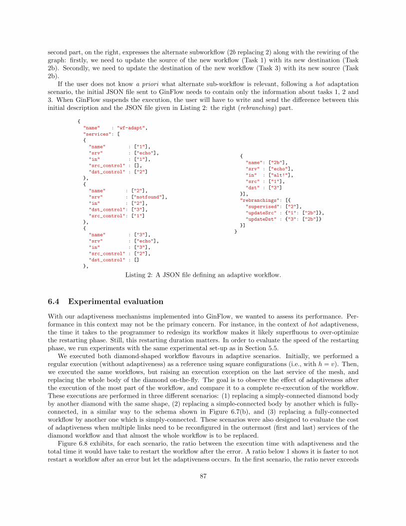
second part, on the right, expresses the alternate subworkflow (2b replacing 2) along with the rewiring of thegraph: firstly, we need to update the source of the new workflow (Task 1) with its new destination (Task2b). Secondly, we need to update the destination of the new workflow (Task 3) with its new source (Task2b).
If the user does not know a priori what alternate sub-workflow is relevant, following a hot adaptationscenario, the initial JSON file sent to GinFlow needs to contain only the information about tasks 1, 2 and3. When GinFlow suspends the execution, the user will have to write and send the difference between thisinitial description and the JSON file given in Listing 2: the right (rebranching) part.
{
"name" : "wf-adapt",
"services": [
{
"name" : ["1"],
"srv" : ["echo"],
"in" : ["1"],
"src_control" : [],
"dst_control" : ["2"]
},
{
"name" : ["2"],
"srv" : ["notfound"],
"in" : ["2"],
"dst_control": ["3"],
"src_control": ["1"]
},
{
"name" : ["3"],
"srv" : ["echo"],
"in" : ["3"],
"src_control" : ["2"],
"dst_control" : []
},
{
"name": ["2b"],
"srv" : ["echo"],
"in" : ["alt!"],
"src" : ["1"],
"dst" : ["3"]
}],
"rebranchings": [{
"supervised": ["2"],
"updateSrc" : {"1": ["2b"]},
"updateDst" : {"3": ["2b"]}
}]
}
Listing 2: A JSON file defining an adaptive workflow.
6.4 Experimental evaluation
With our adaptiveness mechanisms implemented into GinFlow, we wanted to assess its performance. Per-formance in this context may not be the primary concern. For instance, in the context of hot adaptiveness,the time it takes to the programmer to redesign its workflow makes it likely superfluous to over-optimizethe restarting phase. Still, this restarting duration matters. In order to evaluate the speed of the restartingphase, we run experiments with the same experimental set-up as in Section 5.5.
We executed both diamond-shaped workflow flavours in adaptive scenarios. Initially, we performed aregular execution (without adaptiveness) as a reference using square configurations (i.e., with h = v). Then,we executed the same workflows, but raising an execution exception on the last service of the mesh, andreplacing the whole body of the diamond on-the-fly. The goal is to observe the effect of adaptiveness afterthe execution of the most part of the workflow, and compare it to a complete re-execution of the workflow.These executions are performed in three different scenarios: (1) replacing a simply-connected diamond bodyby another diamond with the same shape, (2) replacing a simple-connected body by another which is fully-connected, in a similar way to the schema shown in Figure 6.7(b), and (3) replacing a fully-connectedworkflow by another one which is simply-connected. These scenarios were also designed to evaluate the costof adaptiveness when multiple links need to be reconfigured in the outermost (first and last) services of thediamond workflow and that almost the whole workflow is to be replaced.
Figure 6.8 exhibits, for each scenario, the ratio between the execution time with adaptiveness and thetotal time it would have take to restart the workflow after the error. A ratio below 1 shows it is faster to notrestart a workflow after an error but let the adaptiveness occurs. In the first scenario, the ratio never exceeds
87

1. In other words, adaptiveness, in the worst case where every service (except the final one) needs to bereplayed, is quicker than a complete re-execution whose time is at least twice the execution of the workflowwithout adaptiveness. The second scenario shows that for configurations bigger than 1× 1 the adaptivenessratio remains in the same order, below 1, in spite of the significant number of links to reconfigure and theinvolved services (up to 21× 21). Finally, the third scenario shows that the ratio remains also constant andbelow 1.
6.5 Adapting the workflow shape in literature
While many workflow manager systems initiatives achieve some enactment flexibility at the infrastructurelevel, through for instance re-submissions strategies [67], pilot jobs [28] and task replications [48]), otherworks [99, 58] explicitly deal with adaptiveness for scientific workflows at the application level. In [99],authors propose two patterns to manage the exception handling based on the Reference Nets-within-Netsformalism: propagation and replacement. These mechanisms for dynamically adapting the workflow struc-ture at run time rely on a workflow representation model where the original workflow scenario is mixedwith the alternative path. FireWorks [58] also provides a dynamic feature to add new components to theworkflow while it is running. This workflow manager targets the same use-cases failures as GinFlow but ina less-general way in the sense that they support only what we refer to as cold adaptation.
1x1 6x6 11x11 16x16 21x21configuration
0.0
0.2
0.4
0.6
0.8
1.0
rati
o
Simple to simple
Simple to full
Full to simple
Figure 6.8: With-adaptiveness-over-without-adaptiveness ratio.
88

6.6 Conclusion
We designed an adaptiveness mechanism aiming at helping the workflow designer dealing with the uncertainnature of any computational science venture. The feature designed, developed and experimented allowsthe workflow designer to specify alternate subworkflows either prior to running the workflow or during theworkflow, when the execution manager raises an exception. The adaptation from the initial workflow to thealternative one will get enacted transparently for the user.
Specified using HOCL and intended to run in decentralised settings, this mechanism was implemented inGinFlow and its extra cost at run time was shown to be zero most of the time for diamond-shaped workflowsmade of up to 443 services out of which 441 are adapted and replaced by another set of 441 services.
89


Conclusion
An exploration . . .
The initial motivation behind this series of works as well as our early contributions have been presented onlyin Chapter 5. They were directed towards the proposal of an architecture to decentralise the coordinationof composite services following the observation that, as stated in Chapter , component models, which havebeen recently promising models to compose services and execute them in decentralised settings, are not builtupon abstractions that easily support loose coupling and adaptation.
In our quest for alternative models to enact and adapt composite services in decentralised settings,as it has been detailed throughout this dissertation, HOCL acted as both a source of inspiration and animplementation tool. I do not argue that HOCL, and more generally, chemically-inspired programmingstyles, and even more generally, higher-order rule-based models, are the definite way to program servicecompositions. This series of work appears to me as being part of an exploration that could be summarizedas follows: It appears that the abstractions conveyed by HOCL could help in our quest for programming stylesfor large scale adaptive platforms, let us see where it leads if we assume it is true. The question whether itis actually the right way to go is beyond the scope of this work, and anyway, I believe, not a particularlyrelevant question.
The fact that this work is more exploratory than a large proportion of research work carried out inworkflow computing constitutes both its weakness and its strength. This is a weakness mostly because thereis no precise metric that could establish whether our approach outperforms others. Still, I am not surewhether it would actually makes sense to compare our approach with others performance-wise. Also, ourcontributions are a bit more difficult to position in the state of the art, in the sense that they are not theresult of incremental steps only, but the outcome of more alternative research. While alternative ventures inresearch might carry higher risks of failure, in particular due to their difficulty of positioning, they are morelikely to bring a fresh eye on to some problem at stake.
I believe the out-of-the-mainstream aspect of this work constitutes a strength, because HOCL actuallymakes the workflow shape adaptation possible. I am not saying that there is no other way to achieve it. Ijust think HOCL inspired us on how to do it. More generally, this work conveys the idea that these modelscan be of great help when there is a need for specifying adaptive systems, and we wanted to show it througha concrete example, from the design to some experimental evaluation. May it be inspirational to otherresearchers.
Exploring alternative approaches come with nice opportunities to revisit classical problems. This is whathappened to us when trying to implement a distributed HOCL runtime. We had to revisit the classicalresource allocation problem. So, it was a double inspiration. Firstly, HOCL helped us tackling the decen-tralised adaptive workflow execution problem. Secondly, it allowed us to revisit some classical distributedsystems problems, adding (or relaxing) constraints brought about by its implementation in large distributedsettings. Note that this idea of having protocols that dynamically and locally adapt back-and-forth betweenan optimistic approach and a pessimistic approach can be seen as an application of the vision conveyed byautonomic computing since a few years.
91
. . . with concrete outcomes . . .
Relying over out-of-the-mainstream concepts did not prevent us to make a few concrete contributions. Evenif they were extensively discussed in the technical chapters of this dissertation, let us summarize them andrefer the reader to their related publications. These contributions can be classified into two categories.
The first category of contributions gathers results around the ability to execute workflows in decentralisedsettings in an adaptive manner, subjects of Chapters 5 and 6. They are contributions to the field of workflowmanagement, with ideas echoing the autonomic computing paradigm. This is where HOCL was used as aninspiration, to propose an architecture for a distributed workflow engine, to specify it, and to build a softwareprototype of it, initially called HOCL-TS. The initial proposal for an architecture and the specification of anHOCL-based execution engine was made in [45]. Some early experiments testing the viability of the approachconducted through the deployment of HOCL-TS are reported in [46] and [47]. The extension of these workswith adaptiveness is presented in [87], as well as the refactoring, cleaning and extension of HOCL-TS intoGinFlow, a now ready-to-be-used workflow execution manager whose code has been released in 2015.
The second category of contributions deals with the study of the model itself. On one hand, its complexityhas been more precisely captured — the subject of Chapter 2 and paper [19] —, and on the other hand,its implementation in distributed settings has been studied, — matter of Chapters 3 and 4. In this laststream of research, the contributions are i) the proposal of an adaptive resource allocation algorithm —presented in detail in [17] —, ii) the design of two distributed environments supporting the execution ofprograms written in the chemical style, lifting a barrier towards the use of such models at large scale. Thedesign, implementation and experimental validation of the hierarchical and flat reactors are presented in [79]and [78], respectively.
. . . to be continued . . .
GinFlow has recently been equipped with a graphical interface to specify workflows to be submitted to theworkflow engine. It is particularly useful to deal with hot adaptation.
A planned action for GinFlow is to find more use cases for the adaptiveness feature. In particular,several cosmology codes and their particular usage have been identified as potential benefiters of GinFlow.The first one is Gadget [95], a code for cosmological simulations of structure formation which requires thecosmologist to run an entire simulation and analyse the results to start a second one with the parametersupdated according to the results of the first one. This kind of refinement process could benefit from theGinFlow adaptation mechanisms. Another cosmology project which could leverage GinFlow’s adaptivenessis the Supernova Factory code, aiming at measuring the expansion history of the Universe and explore thenature of Dark Energy [5].
Note that GinFlow has been interfaced with the Tigres workflow runtime system [84], developed atLawrence Berkeley National Lab (LBL). Tigres aims first at providing a set of programming abstractionsto ease the integration of workflow patterns into scientific codes. The supported templates are sequences,parallel splits, forks and joins. The goal of the binding between Tigres and GinFlow was to extend Tigres’potential execution platforms through decentralisation. In this binding, each template is sent to GinFlow,which executes it and sends the output of the template back to the Tigres runtime, which can then moveforward in the execution. Details of the design of this bridge can be found in [86].
. . . for the people
The application space where the programming model conveyed by workflows is useful is much broader thanscience. As we mentioned at the beginning of this document, the early efforts towards programming servicecompositions came from industry. The workflow paradigm is now moving to the every day life, with the
92

apparition of tools helping people to build their own compositions (or recipes) involving services such asemailing, micro-blogging, social networking, and storage management.
IFTTT (If that, then this) is a tool [3] that provides a nice graphical interface to create and use theserecipes such as check the weather, and if it is fine, notify me and find me the closest ice-cream parlor. InApril 2016, Microsoft Flow [4] which provides similar features, went live. Workflows that can be defined withMicrosoft Flow includes many (cloud-based) services such as Slack, Github and Dropbox. While such a toolis very appealing, it comes with the necessity to trust the coordinating third-party: the Microsoft flow server,on which our workflows are stored and managed. (The first mandatory thing to do when trying MicrosoftFlow is to open an account on the Microsoft Flow server). This leads us back to our initial concerns withcentralisation. What these trusted third-parties do with our data is never mentioned when one opens anaccount.
Until recently, many services used in every day life worked due to the presence of a trusted third party.Two common examples are banking and notary certification. In the case of banking, the need is to avoiddouble spending of the same money and thus certify the transaction. Notary certification is useful to ensurethat a document is real in the sense that it was the same when some contract it represents was signed. Thesetwo examples actually rely on one need: time-stamping objects (so they can be ordered in time).
Recently, the blockchain changed this apparently frozen situation by proposing a way to certify trans-actions (and more generally objects) in a decentralised way removing the need for a trusted third-partyauthority. The blockchain was initially proposed in the context of banking, as a way to replace the centralauthority (the banker), by a decentralised cryptographic proof. This allowed the rise of cryptocurrencies,the most known among them being the bitcoin [74], for which these concepts were initially proposed.
The validity of a transaction relies on a proof-of-work. Before it is included into the blockchain (i.e., theofficial ledger), a transaction is first inserted into a block of transactions along with other new transactions.Then, a nonce needs to be found such that it satisfies a hard-to-obtain property: a cryptographic functionapplied on the block and this nonce must return a number which is lower than a given threshold. Findingsuch a nonce requires an amount of computational work which grows inversely to the value threshold. Onceit is found by some node, the block is inserted into the blockchain locally on this node and then sentover the network as the new, up-to-date ledger. In case of several ledgers coexisting in the network, thelongest one is systematically favoured over the smaller ones. This means that an attacker who wants todisseminate a modified ledger needs to build proof-of-works quicker than the honest cooperating nodes inthe network. Consequently, as long as the combined computational power of the honest nodes predominates,the probability of a successful attack is very low.
The threats on privacy brought about by all-powerful centralised services offering social networkingfunctionalities are multiple. Note that, in this context, centralised does not so much refer to the centralisationof the infrastructure than to the fact that a single entity controls it. (Facebook’s few data centers are actuallydistributed across the world.) Trusting such entities to store and expose our data to our friends withoutusing them for their own sake, while this the service is free, appears to be quite irrational, or at least naive.The numerous breaches on personal data recently experienced1 highlight the need for alternate architecturesproviding the same kind of functionalities. This is where decentralised approaches can help. Recently,in the context of social networking, several new platforms and approaches have been proposed to try tofill this gap. A first step towards decentralisation has been achieved by platforms such as Diaspora [1],through a federation of servers, and SuperNova [91] which relies on super-peers to store users’ data. Fullydecentralised approaches were also proposed in the literature, such as Safebook [36], ProofBook [20] andSOUP [62]. These approaches ensures different levels of privacy, anonymity and security in the network,based on decentralisation, cryptographic hashing and proof-of-works. In a recent joint work with Arnaud
1Go to https://en.wikipedia.org/wiki/Data_breach#Major_incidents for a list.
93

Fabre and Marin Bertier, we explored these techniques to propose a decentralised online social network withan emphasis on ensuring anonymity and confidentiality while providing a high level of availability on thedata. Our work also allows users to belong to several groups and share some content with some group whilecompletely hiding it to the others [43].
As can be said about the blockchain, our approach does not need trust to work. More generally, de-centralisation combined with cryptography in a broad sense seems to pave the way for privacy-preservingservice orchestration at large, for the people.
94

Bibliography
[1] Diaspora∗. https://joindiaspora.com/. Retrieved December 2016.
[2] Freepastry. http://www.freepastry.org. Retrieved December 2016.
[3] IFTTT. https://ifttt.com. Retrieved December 2016.
[4] Microsoft flow. https://flow.microsoft.com. Retrieved December 2016.
[5] G. Aldering, G. Adam, P. Antilogus, P. Astier, R. Bacon, S. Bongard, C. Bonnaud, Y. Copin,D. Hardin, F. Henault, D. Howell, J.-P. Lemonnier, J.-M. Levy, S. Loken, P. Nugent, R. Pain, A. Pecon-tal, E. Pecontal, S. Perlmutter, R. Quimby, K. Schahmaneche, G. Smadja, and W. Wood-Vasey.Overview of the Nearby Supernova Factory. SPIE Proceedings Series, 4836:61–72, 2002.
[6] W. R. Ashby. Design for a Brain: The Origin of Adaptive Behavior. Chapman and Hall, 2nd edition,1960.
[7] R. J. Bagley and D. J. Farmer. Spontaneous Emergence of a Metabolism. In C. G. Langton, C. Taylor,D. J. Farmer, and S. Rasmussen, editors, Artificial Life II, pages 93–140, Redwood City, CA, 1992.Addison-Wesley.
[8] J. Banatre and D. Le Metayer. The GAMMA Model and its Discipline of Programming. Sci. Comput.Program., 15(1):55–77, 1990.
[9] J.-P. Banatre, A. Coutant, and D. Le Metayer. A Parallel Machine for Multiset Transformation andits Programming Style. Future Gener. Comput. Syst., 4(2):133–144, Sept. 1988.
[10] J.-P. Banatre, P. Fradet, and D. Le Metayer. Multiset Processing: Mathematical,Computer Science,and Molecular Computing Points of View, chapter Gamma and the Chemical Reaction Model: FifteenYears After, pages 17–44. Springer Berlin Heidelberg, 2001.
[11] J.-P. Banatre, P. Fradet, and Y. Radenac. Generalised Multisets for Chemical Programming. Mathe-matical Structures in Computer Science, 16, 2006.
[12] J.-P. Banatre and D. Le Metayer. Programming by Multiset Transformation. Commun. ACM,36(1):98–111, 1993.
[13] A. Barros, M. Dumas, and P. Oaks. A Critical Overview of the Web Services Choreography DescriptionLanguage. BPTrends, Mar. 2005.
[14] F. Baude, D. Caromel, C. Dalmasso, M. Danelutto, V. Getov, L. Henrio, and C. Perez. GCM: a GridExtension to Fractal for Autonomous Distributed Components. Annales des Telecommunications,64(1-2):5–24, 2009.
[15] BEA, IBM, Interface21, IONA, Oracle, SAP, Siebel, and Sybase. Service Component Architecture -Building Systems using a Service Oriented Architecture - A joint whitepaper. White paper, Nov. 2005.
95
[16] G. Berry and G. Boudol. The Chemical Abstract Machine. In Proceedings of the 17th ACM SIGPLAN-SIGACT Symposium on Principles of Programming Languages, POPL’90, pages 81–94, New York,USA, 1990. ACM.
[17] M. Bertier, M. Obrovac, and C. Tedeschi. Adaptive Atomic Capture of Multiple Molecules. J. ParallelDistrib. Comput., 73(9):1251–1266, Sept. 2013.
[18] M. Bertier, M. Perrin, and C. Tedeschi. On the Complexity of Concurrent Multiset Rewriting. ResearchReport RR-8408, Inria, Dec. 2013. Available at: https://hal.inria.fr/hal-00912554.
[19] M. Bertier, M. Perrin, and C. Tedeschi. On the Complexity of Concurrent Multiset Rewriting. Inter-national Journal of Foundations of Computer Science, 27(1):67–83, 2016.
[20] S. Biedermann, N. P. Karvelas, S. Katzenbeisser, T. Strufe, and A. Peter. ProofBook: An Online SocialNetwork Based on Proof-of-Work and Friend-Propagation. In Proceedings of the 40th InternationalConference on Current Trends in Theory and Practice of Computer Science (SOSFEM 2014), pages114–125. Springer, 2014.
[21] W. Binder, I. Constantinescu, and B. Faltings. Decentralized Orchestration of Composite Web Services.In Proceedings of the 4th IEEE International Conference on Web Services, Chicago, Sept. 2006.
[22] H. Bouziane, C. Perez, and T. Priol. A Software Component Model with Spatial and Temporal Com-positions for Grid Infrastructures. In 14th International Euro-Par Conference on Parallel Processing(Euro-Par 2008), pages 698–708, Las Palmas de Gran Canaria, Spain, Aug. 2008.
[23] I. Brito. Synchronous, Asynchronous and Hybrid Algorithms for DisCSP. In M. Wallace, editor,Proceedings of the 10th International Conference on Principles and Practice of Constraint Programming(CP 2004), volume 3258 of Lecture Notes in Computer Science, pages 791–791. Springer, 2004.
[24] E. Bruneton, T. Coupaye, M. Leclercq, V. Quema, and J. Stefani. The FRACTAL Component Modeland its Support in Java. Softw., Pract. Exper., 36(11-12):1257–1284, 2006.
[25] P. A. Buhler and J. M. Vidal. Enacting BPEL4WS Specified Workflows with Multiagent Systems. InProceedings of the 2nd Workshop on Web Services and Agent-Based Engineering, July 2004.
[26] K. Candan, J. Tatemura, D. Agrawal, and D. Cavendish. On Overlay Schemes to Support Point-in-range Queries for Scalable Grid Resource Discovery. Fifth IEEE International Conference on Peer-to-Peer Computing (P2P’05), 2005.
[27] F. Cappello, E. Caron, M. Dayde, F. Desprez, Y. Jegou, P. Primet, E. Jeannot, S. Lanteri, J. Leduc,N. Melab, G. Mornet, R. Namyst, B. Quetier, and O. Richard. Grid’5000: a Large Scale and HighlyReconfigurable Grid Experimental Testbed. Proceedings of the 6th IEEE/ACM International Workshopon Grid Computing, 2005.
[28] A. Casajus, R. Graciani, S. Paterson, and A. Tsaregorodtsev. DIRAC pilot framework and the DIRACWorkload Management System. Journal of Physics: Conference Series, 219(6), 2010.
[29] K. M. Chandy and J. Misra. The Drinking Philosophers Problem. ACM Transactions on ProgrammingLanguages and Systems, 6(4):632–646, 1984.
[30] A. Chatalic, M. Bertier, and C. Tedeschi. Efficient Execution of Chemically-Inspired Programs UsingGossip Protocols. internship report, Ecole normale superieure de Rennes, 2013. Retrieved in De-cember 2016 at http://perso.eleves.ens-rennes.fr/~achatali/res/rapport_stage_mit1.pdf.In French.
[31] D. Cohen and J. M. Filho. Introducing a Calculus for Higher-Order Multiset Programming. In FirstInternational Conference on Coordination Languages and Models (COORDINATION’96), pages 124–141, Cesena, Italy, Apr. 1996.
96

[32] D. Conte, P. Foggia, C. Sansone, and M. Vento. Thirty Years of Graph Matching in Pattern Recogni-tion. International Journal of Pattern Recognition and Artificial Intelligence, 18(3):265–298, 2004.
[33] S. A. Cook. The Complexity of Theorem-Proving Procedures. In Proceedings of the 3rd Annual ACMSymposium on Theory of Computing (STOC), pages 151–158, Shaker Heights, USA, May 1971.
[34] S. B. Cooper. Computability Theory. Chapman and Hall, 2003.
[35] C. Creveuil. Research Directions in High-Level Parallel Programming Languages, chapter Implemen-tation of Gamma on the connection machine, pages 219–230. Springer Berlin Heidelberg, 1992.
[36] L. A. Cutillo, R. Molva, and T. Strufe. Safebook: A Privacy-Preserving Online Social Network Lever-aging on Real-Life Trust. IEEE Communications Magazine, 47(12):94–101, 2009.
[37] A. Denis, C. Perez, T. Priol, and A. Ribes. Padico: A Component-Based Software Infrastructure forGrid Computing. In 17th International Parallel and Distributed Processing Symposium (IPDPS’03),Nice, France, Apr. 2003.
[38] C. Di Napoli, M. Giordano, Z. Nemeth, and N. Tonellotto. Adaptive Instantiation of Service WorkflowsUsing a Chemical Approach. In Proceedings of the 16th International Euro-Par Conference on ParallelProcessing, Ischia, Italy, Aug. 2010.
[39] P. Dittrich, J. Ziegler, and W. Banzhaf. Artificial chemistries – a Review. Artificial Life, 7:225–275,June 2001.
[40] A. Doniec, S. Piechowiak, and R. Mandiau. A DisCSP Solving Algorithm Based on Sessions. InI. Russell and Z. Markov, editors, 18th International Florida Artificial Intelligence Research SocietyConference (FLAIRS), pages 666–670. AAAI Press, 2005.
[41] P. Downes, O. Curran, J. Cunniffe, and A. Shearer. Distributed Radiotherapy Simulation with theWebcom Workflow System. Int. J. High Perform. Comput. Appl., 24:213–227, 2010.
[42] T. B. Downing. Java RMI: Remote Method Invocation. IDG Books Worldwide, 1st edition, 1998.
[43] A. Fabre, M. Bertier, and C. Tedeschi. Distributed Algorithms for Personal Data Management. Masterthesis, Universite de Rennes 1, 2016. In french.
[44] H. Fernandez. Flexible Coordination Based on the Chemical Metaphor for Service Infrastructures. PhDthesis, Universite de Rennes 1, May 2012.
[45] H. Fernandez, T. Priol, and C. Tedeschi. Decentralized Approach for Execution of Composite WebServices Using the Chemical Paradigm. In 8th International Conference on Web Services (ICWS),pages 139–146, 2010.
[46] H. Fernandez, C. Tedeschi, and T. Priol. Rule-driven Service Coordination Middleware for ScientificApplications. Future Generation Computer Systems, 35:1–13, 2014.
[47] H. Fernandez, C. Tedeschi, and T. Priol. A Chemistry-Inspired Workflow Management System for aDecentralized Workflow Execution. IEEE Transactions on Services Computing, 9(2):213–226, 2016.
[48] R. Ferreira da Silva, T. Glatard, and F. Desprez. Self-Healing of Workflow Activity Incidents onDistributed Computing Infrastructures. Future Generation Computer Systems, 29(8):2284–2294, 2013.
[49] W. Fontana and L. W. Buss. The Arrival of the Fittest: Toward a Theory of Biological Organization.Bulletin of Mathematical Biology, 56(1):1–64, 1994.
[50] D. Gelernter. Generative Communication in Linda. ACM Trans. Program. Lang. Syst., 7(1):80–112,1985.
97

[51] J. Giavitto, O. Michel, and A. Spicher. Spatial Organization of the Chemical Paradigm and theSpecification of Autonomic Systems. In Software-Intensive Systems and New Computing Paradigms -Challenges and Visions, volume 5380 of Lecture Notes in Computer Science, pages 235–254. Springer,2008.
[52] Y. Gil, E. Deelman, M. H. Ellisman, T. Fahringer, G. Fox, D. Gannon, C. A. Goble, M. Livny,L. Moreau, and J. Myers. Examining the Challenges of Scientific Workflows. IEEE Computer,40(12):24–32, 2007.
[53] T. Glatard, J. Montagnat, D. Lingrand, and X. Pennec. Flexible and Efficient Workflow Deploymentof Data-Intensive Applications On Grids With MOTEUR. Int. J. High Perform. Comput. Appl.,22(3):347–360, 2008.
[54] S. Grumbach and F. Wang. Netlog, a Rule-Based Language for Distributed Programming. In 12th In-ternational Symposium on Practical Aspects of Declarative Languages (PADL), volume 5937 of LectureNotes in Computer Science, pages 88–103, Madrid, Spain, Jan. 2010. Springer.
[55] F. Hayes-Roth. Rule-Based Systems. Communications of the ACM, 28(9):921–932, Sept. 1985.
[56] B. Hindman, A. Konwinski, M. Zaharia, A. Ghodsi, A. D. Joseph, R. Katz, S. Shenker, and I. Stoica.Mesos: A Platform for Fine-grained Resource Sharing in the Data Center. In Proceedings of the 8thUSENIX Conference on Networked Systems Design and Implementation, Boston, USA, Apr. 2011.
[57] IBM. An Architectural Blueprint for Autonomic Computing. White paper, June 2005.
[58] A. Jain, S. P. Ong, W. Chen, B. Medasani, X. Qu, M. Kocher, M. Brafman, G. Petretto, G.-M.Rignanese, G. Hautier, D. Gunter, and K. A. Persson. FireWorks: a Dynamic Workflow SystemDesigned for High-Throughput Applications. Concurrency and Computation: Practice and Experience,27(17):5037–5059, 2015.
[59] M. Jelasity, A. Montresor, and O. Babaoglu. Gossip-based Aggregation in Large Dynamic Networks.ACM Trans. Comput. Syst., 23(3):219–252, Aug. 2005.
[60] K. Jensen and L. M. Kristensen. Coloured Petri Nets: Modelling and Validation of Concurrent Systems.Springer, 1st edition, 2009.
[61] A.-M. Kermarrec and M. van Steen. Gossiping in Distributed Systems. SIGOPS Oper. Syst. Rev.,41(5):2–7, Oct. 2007.
[62] D. Koll, J. Li, and X. Fu. Soup: an Online Social Network by the People, for the People. In 15thInternational ACM/IFIP/USENIX Middleware Conference, pages 193–204. ACM, 2014.
[63] H. Kuchen and K. Gladitz. Parallel Implementation of Bags. In Proceedings of the Conference onFunctional Programming Languages and Computer Architecture, FPCA’93, pages 299–307, New York,USA, 1993. ACM.
[64] J. Larrosa and G. Valiente. Constraint Satisfaction Algorithms for Graph Pattern Matching. Mathe-matical. Structures in Comp. Sci., 12(4):403–422, Aug. 2002.
[65] D. Le Metayer. Higher-Order Multiset Programming. In Proceedings of the DIMACS workshop onspecifications of parallel algorithms, DIMACS series in Discrete Mathematics. American MathematicalSociety, 1994.
[66] H. Lin, J. Kemp, and P. Gilbert. Computing Gamma Calculus on Computer Cluster. InternationalJournal of Technology Diffusion, 1(4):42–52, 2010.
98

[67] D. Lingrand, J. Montagnat, and T. Glatard. Modeling User Submission Strategies on ProductionGrids. In Proceedings of the 18th ACM International Symposium on High Performance DistributedComputing, Munich, Germany, June 2009.
[68] J. W. Lloyd. Practical Advantages of Declarative Programming. In Proceedings of the 1994 JointConference on Declarative Programming (GULP-PRODE’94), pages 18–30.
[69] B. Ludascher, I. Altintas, C. Berkley, D. Higgins, E. Jaeger, M. Jones, E. A. Lee, J. Tao, andY. Zhao. Scientific Workflow Management and the Kepler System. Concurrency Comput.: Pract.Exper., 18(10):1039–1065, 2006.
[70] N. A. Lynch, D. Malkhi, and D. Ratajczak. Atomic Data Access in Distributed Hash Tables. InRevised Papers from the First International Workshop on Peer-to-Peer Systems, IPTPS’01, pages295–305, London, UK, 2002. Springer-Verlag.
[71] D. Martin, D. Wutke, and F. Leymann. A Novel Approach to Decentralized Workflow Enactment.In Proceedings of the 12th International IEEE Enterprise Distributed Object Computing Conference,Munich, Germany, Sept. 2008.
[72] B. T. Messmer and H. Bunke. Subgraph Isomorphism in Polynomial Time. Research report, Institutfur Informatik und angewandte Mathematik, University of Bern, Switzerland, 1995.
[73] R. A. Micillo, S. Venticinque, N. Mazzocca, and R. Aversa. An Agent-Based Approach for DistributedExecution of Composite Web Services. In Proceedings of the 17th IEEE International Workshops onEnabling Technologies, Rome, Italy, June 2008.
[74] S. Nakamoto. Bitcoin: A Peer-to-Peer Electronic Cash System. https://bitcoin.org/bitcoin.pdf,2009. Retrieved December 2016.
[75] Z. Nemeth, C. Perez, and T. Priol. Workflow Enactment Based on a Chemical Methaphor. In Proceed-ings of the 3rd IEEE International Conference on Software Engineering and Formal Methods, Koblenz,Germany, Sept. 2005.
[76] R. D. Nicola, G. Ferrari, and R. Pugliese. KLAIM: A Kernel Language for Agents Interaction andMobility. IEEE Trans. Softw. Eng., 24(5):315–330, 1998.
[77] M. Obrovac. Chemical Computing for Distributed Systems: Algorithms and Implementation. PhDthesis, Universite de Rennes 1, Mar. 2013.
[78] M. Obrovac and C. Tedeschi. Deployment and Evaluation of a Decentralised Runtime for ConcurrentRule-Based Programming Models. In 14th International Conference on Distributed Computing andNetworking (ICDCN 2013), volume 7730, pages 408–422, Bombay, India, January, 3-6 2013.
[79] M. Obrovac and C. Tedeschi. Distributed Chemical Computing: A Feasibility Study. InternationalJournal of Unconventional Computing, 9(3-4):203–236, 2013.
[80] M. Parashar and S. Hariri. Autonomic Computing: An Overview. In International Workshop onUnconventional Programming Paradigms (UPP), pages 257–269, Le Mont Saint-Michel, France, Sept.2004.
[81] G. Paun, G. Rozenberg, and A. Salomaa. The Oxford Handbook of Membrane Computing. OxfordUniversity Press, Inc., New York, USA, 2010.
[82] M. J. Quinn. Parallel Programming in C with MPI and OpenMP. McGraw-Hill Education Group,2003.
[83] Y. Radenac. Programmation “chimique” d’ordre superieur. PhD thesis, Universite de Rennes 1, April2007.
99

[84] L. Ramakrishnan, S. S. Poon, V. Hendrix, D. K. Gunter, G. Z. Pastorello, and D. A. Agarwal. Ex-periences with User-Centered Design for the Tigres Workflow API. In Proceedings of the 10th IEEEInternational Conference on e-Science, pages 290–297. IEEE Computer Society, Oct. 2014.
[85] M. Raynal. A Distributed Solution to the k-out of-M Resources Allocation Problem. In Advances inComputing and Information — ICCI’91, volume 497 of Lecture Notes in Computer Science. Springer,1991.
[86] J. Rojas Balderrama, M. Simonin, C. Morin, V. Hendrix, L. Ramakrishnan, D. Agarwal, andC. Tedeschi. Combining Workflow Templates with a Shared Space-based Execution Model. In Pro-ceedings of the 9th Workshop on Workflows in Support of Large-Scale Science, New Orleans, LA, Nov.2014.
[87] J. Rojas Balderrama, M. Simonin, and C. Tedeschi. GinFlow: A Decentralised Adaptive Workflow Exe-cution Manager. In 30th IEEE International Parallel and Distributed Processing Symposium (IPDPS),Chicago, USA, May 23-27 2016.
[88] A. I. T. Rowstron and P. Druschel. Pastry: Scalable, Decentralized Object Location, and Routingfor Large-Scale Peer-to-Peer Systems. In Proceedings of the IFIP/ACM International Conference onDistributed Systems Platforms (Middleware’01), pages 329–350, London, UK, 2001. Springer-Verlag.
[89] C. Schmidt and M. Parashar. Squid: Enabling Search in DHT-based Systems. J. Parallel Distrib.Comput., 68(7):962–975, 2008.
[90] F. B. Schneider. Implementing Fault-Tolerant Services Using the State Machine Approach: a Tutorial.ACM Comput. Surv., 22, 1990.
[91] R. Sharma and A. Datta. Supernova: Super-Peers Based Architecture for Decentralized Online SocialNetworks. In 4th International Conference on Communication Systems and Networks (COMSNETS),pages 1–10. IEEE, 2012.
[92] J. Siegel. CORBA 3 Fundamentals and Programming. John Wiley & Sons, Inc., New York, USA, 2ndedition, 1999.
[93] D. Skeen and M. Stonebraker. A Formal Model of Crash Recovery in a Distributed System. IEEETransactions on Software Engineering, SE-9(3), 1983.
[94] M. Sonntag, K. Gorlach, D. Karastoyanova, F. Leymann, and M. Reiter. Process Space-based ScientificWorkflow Enactment. International Journal of Business Process Integration and Management, 5(1):32–44, 2010.
[95] V. Springel. The Cosmological Simulation Code GADGET-2. Monthly Notices of the Royal Astro-nomical Society, 364:1105–1134, 2005.
[96] I. Stoica, R. Morris, D. Karger, M. F. Kaashoek, and H. Balakrishnan. Chord: A Scalable Peer-to-peerLookup Service for Internet Applications. In Proceedings of the 2001 ACM Conference on Applications,Technologies, Architectures, and Protocols for Computer Communications (SIGCOMM’01), pages 149–160, 2001.
[97] Y. Suzuki and H. Tanaka. Symbolic Chemical System Based on Abstract Rewriting System and itsBehavior Pattern. Artificial Life and Robotics, 1:211–219, 1997.
[98] C. Szyperski. Component Software: Beyond Object-Oriented Programming - 2nd edition. Addison-Wesley, 2002.
[99] R. Tolosana-Calasanz, J. A. Banares, O. F. Rana, P. Alvarez, J. Ezpeleta, and A. Hoheisel. AdaptiveException Handling for Scientific Workflows. Concurrency Comput.: Pract. Exper., 22(5):617–642,2010.
100

[100] A. M. Turing. On Computable Numbers, with an Application to the Entscheidungsproblem. Proceed-ings of the London Mathematical Society. Second Series, 42:230–265, 1936.
[101] J. R. Ullmann. An Algorithm for Subgraph Isomorphism. J. ACM, 23(1):31–42, Jan. 1976.
[102] J. von Neumann. First Draft of a Report on the EDVAC. IEEE Ann. Hist. Comput., 15(4):27–75,Oct. 1993.
[103] K. Wolstencroft, R. Haines, D. Fellows, A. Williams, D. Withers, S. Owen, S. Soiland-Reyes, I. Dunlop,A. Nenadic, P. Fisher, J. Bhagat, K. Belhajjame, F. Bacall, A. Hardisty, A. Nieva de la Hidalga, M. P.Balcazar Vargas, S. Sufi, and C. Goble. The Taverna Workflow Suite: Designing and ExecutingWorkflows of Web Services on the Desktop, Web or in the Cloud. Nucleic Acids Res., 41(Webserver-Issue):557–561, 2013.
[104] W. Yu. Consistent and Decentralized Orchestration of BPEL Processes. In Proceedings of the 24thACM Symposium on Applied Computing (SAC), Honolulu, Mar. 2009.
[105] R. Zivan and A. Meisels. Parallel Backtrack Search on DisCSP. In Proceedings of the Workshop onDistributed Constraint Reasoning (DCR-02), Bologna, Italy, 2002.
[106] R. Zivan and A. Meisels. Message Delay and DisCSP Search Algorithms. Annals of Mathematics andArtificial Intelligence, 46(4):415–439, Apr. 2006.
101