Embed Size (px)
Citation preview

c©Copyright 2012
Towfiq Ahmed


Hubbard Model Approach to X-ray Spectroscopy
Towfiq Ahmed
A dissertationsubmitted in partial fulfillment of the
requirements for the degree of
Doctor of Philosophy
University of Washington
2012
Reading Committee:
John J. Rehr, Chair
Gerald T. Seidler
Anton Andreev
Program Authorized to Offer Degree:UW Department of Physics


University of Washington
Abstract
Hubbard Model Approach to X-ray Spectroscopy
Towfiq Ahmed
Chair of the Supervisory Committee:
Professor John J. RehrDepartment of Physics
We have implemented a Hubbard model based first-principles approach for real-space calculations
of x-ray spectroscopy, which allows one to study excited state electronic structure of correlated
systems. Theoretical understanding of many electronic features ind and f electron systems remains
beyond the scope of conventional density functional theory(DFT). In this work our main effort is to
go beyond the local density approximation (LDA) by incorporating the Hubbard model within the
real-space multiple-scattering Green’s function (RSGF) formalism. Historically, the first theoretical
description of correlated systems was published by Sir Neville Mott and others in 1937. They
realized that the insulating gap and antiferromagnetism inthe transition metal oxides are mainly
caused by the strong on-site Coulomb interaction of the localized unfilled 3d orbitals. Even with
the recent progress of first principles methods (e.g. DFT) and model Hamiltonian approaches (e.g.,
Hubbard-Anderson model), the electronic description of many of these systems remains a non-trivial
combination of both.
X-ray absorption near edge spectra (XANES) and x-ray emission spectra (XES) are very power-
ful spectroscopic probes for many electronic features nearFermi energy (EF ), which are caused by
the on-site Coulomb interaction of localized electrons. Inthis work we focus on three different cases
of many-body effects due to the interaction of localizedd electrons. Here, for the first time, we have
applied the Hubbard model in the real-space multiple scattering (RSGF) formalism for the calcula-
tion of x-ray spectra of Mott insulators (e.g., NiO and MnO).Secondly, we have implemented in our
RSGF approach a doping dependent self-energy that was constructed from a single-band Hubbard


model for the over doped high-Tc cuprate La2−xSrxCuO4. Finally our RSGF calculation of XANES
is calculated with the spectral function from Lee and Hedin’s charge transfer satellite model. For
all these cases our calculated x-ray spectra yield reasonable agreement with experiment. The above
work has been implemented as an extension into the FEFF9 code, and we have also included notes
for the new and modified key features of this development.
Aside from the x-ray spectroscopy of correlated systems, wealso present our calculation of the
ground state local electronic structure of DNA nucleotideson graphene, and the transmission cur-
rents through graphene nanopores. Our calculation and analysis provide theoretical guidelines for
developing DNA sequencing techniques using scanning tunneling spectroscopy (STS) and nanopore
experiment. Evolved as a secondary focus of this thesis, we have added an additional chapter dis-
cussing our calculation of DNA-graphene hybrids.


TABLE OF CONTENTS
Page
List of Figures . . . . . . . . . . . . . . . . . . . . . . . . . . . . . . . . . . . . . .. . . . iii
List of Tables . . . . . . . . . . . . . . . . . . . . . . . . . . . . . . . . . . . . . . .. . . v
Glossary . . . . . . . . . . . . . . . . . . . . . . . . . . . . . . . . . . . . . . . . . . .. . vi
Chapter 1: Introduction . . . . . . . . . . . . . . . . . . . . . . . . . . . . . .. . . . 1
1.1 Historical Background . . . . . . . . . . . . . . . . . . . . . . . . . . . .. . . . 1
1.2 Goal of the Dissertation . . . . . . . . . . . . . . . . . . . . . . . . . . .. . . . . 3
1.3 Overview of the Dissertation . . . . . . . . . . . . . . . . . . . . . . .. . . . . . 4
1.4 Units and Convention . . . . . . . . . . . . . . . . . . . . . . . . . . . . . .. . . 5
1.5 Review of x-ray spectroscopy . . . . . . . . . . . . . . . . . . . . . . .. . . . . . 5
Chapter 2: Background Theory . . . . . . . . . . . . . . . . . . . . . . . . . .. . . . 7
2.1 Real-space Green’s function theory . . . . . . . . . . . . . . . . .. . . . . . . . . 7
2.2 Multiple-scattering formalism for x-ray spectroscopy. . . . . . . . . . . . . . . . 11
2.3 Density Functional Theory and GW Approximation . . . . . . .. . . . . . . . . . 12
2.4 Theory of localized electrons and strong correlation . .. . . . . . . . . . . . . . . 17
Chapter 3: Hubbard model corrections in real-space x-ray spectroscopy theory . . . . . 20
3.1 Introduction . . . . . . . . . . . . . . . . . . . . . . . . . . . . . . . . . . . .. . 21
3.2 Hubbard model in Real-space Green’s function Theory . . .. . . . . . . . . . . . 23
3.3 ab initio Hubbard parameters using constrained RPA . . . . . . . . . . . . . . .. 27
3.4 Electron self-energy . . . . . . . . . . . . . . . . . . . . . . . . . . . . .. . . . . 29
3.5 Density of States . . . . . . . . . . . . . . . . . . . . . . . . . . . . . . . . .. . 32
3.6 X-ray spectroscopy . . . . . . . . . . . . . . . . . . . . . . . . . . . . . . .. . . 37
3.7 Conclusion . . . . . . . . . . . . . . . . . . . . . . . . . . . . . . . . . . . . . .41
Chapter 4: X-ray absorption near-edge spectra of overdopedLSCO . . . . . . . . . . . 45
4.1 Introduction . . . . . . . . . . . . . . . . . . . . . . . . . . . . . . . . . . . .. . 46
i

4.2 Fermi-liquid description of La2−xSrxCuO4 . . . . . . . . . . . . . . . . . . . . . . 48
4.3 Doping dependent self-energy in single-band Hubbard model . . . . . . . . . . . . 49
4.4 X-ray spectroscopy of overdoped LSCO . . . . . . . . . . . . . . . .. . . . . . . 50
4.5 Conclusion . . . . . . . . . . . . . . . . . . . . . . . . . . . . . . . . . . . . . .56
Chapter 5: Charge transfer satellites in strongly correlated systems . . . . . . . . . . . 57
5.1 Introduction . . . . . . . . . . . . . . . . . . . . . . . . . . . . . . . . . . . .. . 57
5.2 Lee-Hedin charge transfer satellite model . . . . . . . . . . .. . . . . . . . . . . 58
5.3 Spectral function . . . . . . . . . . . . . . . . . . . . . . . . . . . . . . . .. . . 63
5.4 X-ray spectroscopy of High Tc materials . . . . . . . . . . . . . . . . . . . . . . . 64
5.5 Conclusion . . . . . . . . . . . . . . . . . . . . . . . . . . . . . . . . . . . . . .65
Chapter 6: Other Electronic Structures: DNA-graphene hybrids . . . . . . . . . . . . 67
6.1 Electronic Fingerprints of DNA bases on Graphene . . . . . .. . . . . . . . . . . 67
6.2 Identifying DNA bases with Transport Current . . . . . . . . .. . . . . . . . . . . 74
6.3 Conclusion . . . . . . . . . . . . . . . . . . . . . . . . . . . . . . . . . . . . . .76
Chapter 7: Conclusion . . . . . . . . . . . . . . . . . . . . . . . . . . . . . . . .. . 77
Bibliography . . . . . . . . . . . . . . . . . . . . . . . . . . . . . . . . . . . . . . .. . . 81
Appendix A: LDA+U extension of FEFF: New and Modified Code . . . . . . . . . . . . 90
A.1 Input: feff.inp . . . . . . . . . . . . . . . . . . . . . . . . . . . . . . . . . .. . . 90
A.2 Final output files . . . . . . . . . . . . . . . . . . . . . . . . . . . . . . . . .. . 91
A.3 Intermediate output files . . . . . . . . . . . . . . . . . . . . . . . . . .. . . . . 91
A.4 Modified routines in FEFF90 for LDA+U . . . . . . . . . . . . . . . . . . . . . . 92
A.5 Example input file . . . . . . . . . . . . . . . . . . . . . . . . . . . . . . . . .. . 94
A.6 Program running flow chart . . . . . . . . . . . . . . . . . . . . . . . . . .. . . . 94
Appendix B: Scanning Tunneling Spectroscopy and Local Density of States . . . . . . . 98
B.1 Interaction of Graphene and DNA base . . . . . . . . . . . . . . . . .. . . . . . . 98
B.2 3D Perspective . . . . . . . . . . . . . . . . . . . . . . . . . . . . . . . . . . .. 99
B.3 Calculation Method . . . . . . . . . . . . . . . . . . . . . . . . . . . . . . .. . . 99
ii

LIST OF FIGURES
Figure Number Page
3.1 Calculation ofU for 3d transition metals . . . . . . . . . . . . . . . . . . . . . . . 30
3.2 U dependence on total DOS of MnO . . . . . . . . . . . . . . . . . . . . . . . . . 33
3.3 Angular momentum projectedl -DOS for Mn and O in MnO with and without Hub-bard model . . . . . . . . . . . . . . . . . . . . . . . . . . . . . . . . . . . . . . 34
3.4 U dependence on total DOS of NiO . . . . . . . . . . . . . . . . . . . . . . . . . 36
3.5 Angular momentum projectedl -DOS for Ni and O in NiO with and without Hubbardmodel . . . . . . . . . . . . . . . . . . . . . . . . . . . . . . . . . . . . . . . . . 37
3.6 MnO total DOS with our cRPA calculatedU and GW@LDA+U by Patricket al. [1] 39
3.7 Spin resolved Cud-DOS with and without Hubbard correction . . . . . . . . . . . 40
3.8 Op-DOS in LSCO with and without Hubbard correction . . . . . . . . . .. . . . 41
3.9 O K-edge XAS and XES in MnO with and without Hubbard correction . . . . . . 42
3.10 O K-edge in NiO with and without Hubbard correction . . . .. . . . . . . . . . . 43
3.11 O K-edge XAS and XES for LSCO with and without Hubbard correction . . . . . 44
4.1 Site- andl-projected O DOS in doped LSCO . . . . . . . . . . . . . . . . . . . . . 51
4.2 Theoretical and experimental O K-edge XANES spectra in overdoped LSCO . . . 52
4.3 Cu K-edge XANES spectra in overdoped LSCO . . . . . . . . . . . . .. . . . . . 53
4.4 Doping dependent O K-edge XANES in LSCO . . . . . . . . . . . . . . .. . . . 54
4.5 Oxygen K-edge XANES compared with theoretical single-band p-DOS . . . . . . 55
5.1 Spectral function of NCCO . . . . . . . . . . . . . . . . . . . . . . . . . .. . . . 59
5.2 Spectral function of NCCO . . . . . . . . . . . . . . . . . . . . . . . . . .. . . . 64
5.3 Cu K-Edge XANES of La2−xSrxCuO4 . . . . . . . . . . . . . . . . . . . . . . . . 65
5.4 Cu K-Edge XANES of Nd2−xCexCuO4 . . . . . . . . . . . . . . . . . . . . . . . 66
6.1 Schematic illustration of scanning tunneling spectroscopy . . . . . . . . . . . . . . 68
6.2 Charge density, LDOS and topography of DNA bases on graphene . . . . . . . . . 70
6.3 Fingerprints of DNA bases on graphene from N LDOS . . . . . . .. . . . . . . . 71
6.4 LDOS of DNA bases on graphene with SiC substrate . . . . . . . .. . . . . . . . 73
6.5 Schematic illustration of transmissions through graphene nanopores for DNA fin-gerprinting . . . . . . . . . . . . . . . . . . . . . . . . . . . . . . . . . . . . . . . 74
iii

6.6 Difference curve of the average conductance of isolatedDNA bases inside nanopore 75
6.7 dI/dV andd2I/dV2 of DNA bases through graphene nanopore . . . . . . . . . . 76
A.1 Example of FEFF9 input files with HUBBARD card . . . . . . . . . .. . . . . . 95
A.2 Program flow of “Vanilla-FEFF” stage . . . . . . . . . . . . . . . . .. . . . . . . 96
A.3 Flow chart for intermediate stage where density matrix is diagonalized and Hubbardpotential constructed . . . . . . . . . . . . . . . . . . . . . . . . . . . . . . .. . 96
A.4 Program flow of “Hubbard-FEFF” stage . . . . . . . . . . . . . . . . .. . . . . . 97
B.1 Charge density and atomic structure for four DNA bases ongraphene . . . . . . . 100
B.2 Atomic structure of each nucleobase on graphene. The angle denotes the orientationof each nucleobase. . . . . . . . . . . . . . . . . . . . . . . . . . . . . . . . . . .101
iv

LIST OF TABLES
Table Number Page
3.1 Mnd-state parameters (U = 5.4 eV;J = 0.9 eV) . . . . . . . . . . . . . . . . . . . 35
3.2 Ni d-state parameters (U = 8.0 eV;J = 0.9 eV) . . . . . . . . . . . . . . . . . . . 35
3.3 Calculated Hubbard parameterU and gap∆ of MnO, NiO, and LSCO. . . . . . . 38
B.1 Binding Energy (eV) between DNA bases and Graphene . . . . .. . . . . . . . . 99
v

GLOSSARY
XAS: X-ray absorption spectrum.
XES: X-ray emission spectrum.
XANES: X-ray absorption near edge structure.
DOS: Density of states.
LDOS: L(Angular momentum) projected density of states.
RPA: Random phase approximation.
CRPA: constrained random phase approximation.
RSGF: Real-space Green’s function.
MS: Multiple-scattering.
FMS: Full multiple-scattering.
LDA: Local density approximation.
LSDA: Local spin density approximation.
DFT: Density functional theory.
vi

ACKNOWLEDGMENTS
For the completion of this thesis, I am indebted to many people including my committee mem-
bers, my friends, my family members and my wife.
First I would like to express my deepest gratitude to my advisor, Professor John J. Rehr, for
his excellent guidance, caring, patience, and providing mewith an excellent atmosphere for doing
research. I would then give special thanks to Dr. Joshua Kas for guiding my research for the past
several yeras and helping me to develop my background in various techniques of condensed matter
physics. I learnt lot from our countless hours of physics discussion. Many thanks to Dr. Alexander
Balatsky from LANL for his constant support and guidence in much of the work in my thesis. I
would also like to thank all my committee members including Dr. Gerald T. Seidler, Dr. M.P.
Anantram, Dr. Marcel denNijs, Dr. Alejandro Garcia, annd particularly Dr. Anton Andreev for
willing to participate in my final defense committee at the last moment.
I would like to thank Prof. Arun Bansil from Northeastern University for his insightful guidence
and for giving me the opportunity to collaborate with his Group. Special thanks will go to Dr.
Tanmoy Das, who as a good friend, was always willing to help and give his best suggestions. Thank
you Dr. Fernando Vila and John Vinson for helping me with stimulating discussion whenever I
had trouble with various computation and physics problems.It would have been a lonely office
without you. My gratitude goes to all the other members of Rehr Group for their friendly support
and help. I would also like to thank my mother, three elder sisters, and elder brother. They were
always supporting and encouraging me with their best wishesfrom the furthest end of the planet.
Finally, I would like to thank my wife, Mumu Mahruba Mahbub. She was always there cheering
me up and stood by me through the good times and bad.
vii

DEDICATION
I would like to dedicate this work to my mother Fahmida Hossain and to my wife Mumu Mahbub
who constantly love and support me in each and every step of mylife.
viii

1
Chapter 1
INTRODUCTION
Research in the area of correlated systems has progressed significantly over the last thirty years.
Due to the recent advances in experimental techniques and computing resources, it is now possible
to study a series of exotic materials including heavy fermions, copper-based high temperature super-
conductors and colossal magnetoresistance. With the development of second generation synchrotron
radiation, high resolution x-ray spectroscopy of these systems became possible, and plethora of ex-
citing experimental data became available for theoreticalunderstanding. A growing need to explain
the underlying physics has driven a significant effort to develop theoretical and computational tools
beyond the conventional electronic-structure codes.
There are two main ways one can study ground state propertiesand excitation spectra of many-
electron systems. In the first approach one constructs a parameter-dependent model hamiltonian
where the parameter(s) is fitted with some previously measured experimental data, and the sec-
ond one is a parameter free first principle approach. The mostsuccessful of all the first-principle
approaches is Density Functional Theory (DFT) within the local density approximation (LDA). De-
spite its enormous success in simple metals and molecular systems, the limitation of LDA is clearly
visible for systems with partially filledd or f shells, e.g. transition-metal or rare-earth compounds.
There have been several attempts to improve over LDA such as self-interaction correction (SIC),
GW approximation, LDA+U , dynamical mean-field theory (DMFT) etc. In the present work, a
first-principles Hubbard model approach will be followed within a RSGF multiple-scattering frame
work.
1.1 Historical Background
Despite its relatively recent popularity, the history of strongly correlated systems pre-dates much
of the modern development of many-body quantum theory. One of the early successes of quantum
mechanics was indeed the development of single particle band-structure theory which was able to

2
describe most of the simple metals and a handful of regular insulators. It was about the same time
when interest in metal-insulator transition increased leading to the realization of a new class of
materials. In 1937 de Boer and Verway [2] first pointed out thespecial case of NiO, a transparent
non-metal which should be metallic according to the single-particle band-structure theory. It was
Peierls who, for the first time, proposed the possibility of the strong Coulomb correlation as the
underlying cause of the insulating phase in these systems.
In a series of seminal papers from 1935 to 1949, using a crystalline array of hydrogen-like atoms
with varying lattice constanta, Sir Neville Mott was able to show and classify a class of insulators,
now known as Mott insulators [3, 4]. In such systems, the screened potential around each positive
charge is given by
V(r) = −e2
reqr, (1.1)
where the screening constantq was calculated using Thomas-Fermi model [4, 5]. In this description,
the value ofq was just enough to trap an electron. With varyingq, all trapped electrons in the system
go through a transition where all of them eventually become free. Thus a formal, yet simple metal
to insulator transition was proposed for the first time. In 1951 Slater provided a description [6, 7]
where the anti-ferromagnetic lattices are responsible forthe splitd-bands in NiO or similar systems.
But such systems were later found to remain non-metallic even above Neel temperature where the
AFM ordering vanishes [4].
A next step development came from Hubbard in 1964 with a modelin which the on-site Coulomb
interaction was included while long-range forces are neglected [8, 9]. With large values of the lattice
constanta, this model was able to explain the appearance of antiferromagnetic phases and band
splitting as Slater claimed earlier.
In recent years Lars Hedin and others have shown [10, 11] thatan efficient and consistent treat-
ment of many-body effects are essential for dealing with strong-correlation phenomena. Despite the
enormous success of the quasi-particle GW formalism in semiconducting systems, insulators with
strong Coulomb interaction still remains a challenge.
Some of the of the most successful modern developments for ground state properties of cor-
related systems are the LDA+U by Anisimov et al. [12, 13], SIC method by Perdewet al. [14],
and hybrid functional approach e.g. HSE functional [15]. For excitation properties, TDDFT [16]

3
and configuration interaction CI [17] are still limited to smaller systems. Recent development in
dynamical mean field theory (DMFT) [18] seems promising although computationally expensive.
1.2 Goal of the Dissertation
Almost all efforts to integrate strong correlation effectswith first principles methods end up being
either computationally very expensive or parameter dependent, e.g., relying on HubbardU and
exchangeJ terms. Currently there are a number of ground-state electronic structure codes available
that can incorporate a Hubbard model correction, but the majority of them fit the parameterU
to obtain the experimental band gap. In the presence of strong electron-electron interactions, the
narrow band at the Fermi energy splits into upper and lower Hubbard band and a insulating gap is
formed. Thus, to understand the physics near the Fermi energy of such systems, a good description
of the unoccupied states is essential.
In order to reproduce some of the signature features in the XANES and density of states (DOS)
of Mott insulators, in this thesis we have implemented a rotationally invariant real-space Hubbard
model on top of our real-space multiple-scattering method.This correctly accounts for the onsite
strong Coulomb interaction of the localizedd-orbital electrons, and our calculations show good
agreement with experimentally observed features. Most of the developments presented in this thesis
are within the RSGF framework of the FEFF9 program. As a quasi-particle excited state electronic-
structure code, FEFF9 calculates occupied and unoccupied electronic states as well as various x-ray
spectrum in the presence of the core-hole. Here also we calculate the dominant Hubbard parameter
U within the scope of FEFF9 code. As the main purpose of this work, our development thus compu-
tationally reproduces, from first-principles, the electronic structure and spectral features present in
the x-ray spectra of Mott-Hubbard insulators due to strong onsite Coulomb interaction of localized
3d electrons.
Many correlated-electron systems including the high-Tc cuprates, show doping dependent spec-
tral features in their near edge x-ray spectra. As the dopingconcentration increases, the spectral
features due to strong Coulomb interaction vanishes in manysuch systems, e.g., Nd2−xCexCuO4
(NCCO) and La2−xSrxCuO4 (LSCO). To account for such changes in the correlation strength with
varying doping concentration, a quasi-particle self-energy was originally developed by Bansilet al.

4
[19] using a single-band Hubbard model. As the next topic of this thesis, we have implemented
this self-energy in our RSGF code FEFF, and calculated the doping dependent O K-edge XANES
in over-doped LSCO which are in good accord with experiment.
Another interesting property of correlated systems is the many-body charge-transfer excitations.
The signatures of such excitation are often present in the x-ray spectroscopy, and are generally
identified as the shake-up or shake-down satellites. In thisthesis we have also studied some of
the satellite features present in the Cu K-edge XANES of Nd2CuO4 and La2CuO4. Following the
prescription of Leeet al. [20], we constructed a charge transfer (CT) spectral function. Our RSGF
calculation of XANES convoluted with the CT spectral function yields good agreement with the
experiment by Kosugiet al. [21]
As a secondary interest, we have also applied our first-principles calculation of the local elec-
tronic structure using ground-state DFT and conductance using non-equilibrium Green’s function
(NEGF) technique for the DNA nucleotides on graphene. Our computation, although not directly
connected to the problem of correlated systems, provides theoretical guidelines for scanning tun-
neling spectroscopy (STS) and nano-pore sequencing experiment in the ongoing effort to develop
cheaper and accurate DNA fingerprinting techniques.
1.3 Overview of the Dissertation
The chapters in this thesis are organized as follows: In chapter 1 we briefly make historical remarks
on some of the key developments in our understanding of strongly correlated systems. This chapter
also includes the goal of this work, our key observations, and a quick review of x-ray absorption
and emission spectroscopy. The discussion in chapter 2 provides a review of all the background
concept and theories needed for the rest of the thesis. Starting with the real-space Green’s function
and multiple scattering formalism of x-ray spectroscopy, we briefly discuss some of the key features
of Hubbard model and high temperature superconductivity. The discussion in chapter 3 and 4 are
based on our previously published papers [22, 23]. chapter 3discusses our rotationally invariant
Hubbard model and its implementation in the real-space multiple-scattering code FEFF9. Here we
also briefly discuss our method for the calculation of the Hubbard parameterU . In this chapter
we show our calculation of XANES and DOS of transition metal oxides (NiO, MnO) and High

5
Tc cuprate (LSCO), and compare with experiment. The work presented in chapter 4 stems from a
collaboration between the Rehr Group at University of Washington and the Bansil group at North-
eastern University. In this chapter we discuss the key features of a doping dependent self-energy
which is developed at Northeastern University. We apply this self-energy to our RSGF code FEFF9,
and presented our calculation of O K-edge XANES in over-doped LSCO. chapter 6 is dedicated
to our ground state calculation of DNA nucleotides on graphene and electron transport calculation
through graphene nano-pores.
In chapter 7 we give concluding remarks and briefly discuss future directions. Finally we give a
detailed description of our computer program in appendix-Athat has been developed and added to
FEFF9 as an integrated part of this work. Some supplementarymaterials for chapter 6 are given in
appendix B.
1.4 Units and Convention
In this thesis atomic units are employed for all physical quantities, i.e.,me = 1, |e|= 1, h= 1, where
me is the electron mass,e is the electron charge,h is Plank’s constant divided by 2π. The atomic
unit of length is the bohr,a0 = h2/mee2 ≈ 0.529A. The atomic unit of cross section isa20 ≈ 28.0 Mb,
where a barn (b) equals 10−28m2. The atomic unit of energy is the Hartree,Eh = mee4/h2 ≈ 27.2eV.
In this thesis most of our calculated results are LDOS (angular momentum projected density of
states) and K-edge XANES (x-ray absorption near edge structure) spectra. In FEFF calculations the
XANES spectrum output is normalized within 50 eV of the threshold (edge) energy. In order to
compare with experiments we have scaled the spectrum and hence the y-axis has arbitrary units.
1.5 Review of x-ray spectroscopy
1.5.1 x-ray absorption
For the purpose of this thesis we now briefly discuss a few fundamental concepts of x-ray absorption
(XAS) and x-ray emission (XES) spectra. In XAS, the light with intensityI0 hits the sample with
thicknessl , and according the Beer-Lambert law
I = I0e−µ(E)l . (1.2)

6
This equation can be re-written for theabsorption coefficientas,
µ(E) = −(dI/dl)/I . (1.3)
This coefficient is also related to the scattering cross-section of the absorbing center inside the
material as
µ(E) = σtot(E)na, (1.4)
wherena is the density of scattering atoms in the sample.
The naming convention of the edge in spectroscopy depends onthe type of core-level excitation,
e.g., for the K edge, x-ray excites a 1s electron. The excited electron then fills an unoccupiedp
state following the dipole selection rulel = ±1. Thus the x-ray absorption, and more precisely
the x-ray near edge absorption spectrum (XANES) maps out theunoccupied density of states near
the Fermi energy. In this process the photoelectron sees theeffects of the screened core-hole which
it leaves behind, and the spectrum is broadened by the life time of the core-hole. The absorption
spectrum can be further broadened by the extrinsic and intrinsic losses which are discussed by Luke
Campbell in the context of RSGF method [24].
1.5.2 x-ray emission spectroscopy
In the context of our RSGF code, XES refers to the x-ray emission spectroscopy. In practice, one
can think of XES as an inverse process of XAS where the occupied states below the Fermi energy
fill out an existing hole according to the dipole selection rule. Thus XES maps out the occupied
density of states, including those near the Fermi energy. Inthis process the energy broadening is
negligible since the hole, which was left behind by the electron, is very close to the Fermi energy
and has a much longer life time.

7
Chapter 2
BACKGROUND THEORY
In this chapter we review the background theory which is relevant to our work presented in this
thesis. In general, our development of computational methods for calculating x-ray spectroscopy
of correlated systems, is built on real-space Green’s function (RSGF) theory and a Hubbard model
with an ab initio determination ofU and a many-pole approximation to the GW self-energy. The
multiple scattering formalism of RSGF method is formally equivalent to the much celebrated density
functional theory in many aspects. Both approaches are extendable to a quasiparticle description
by incorporating a GW like approximation. Here we briefly review the GW approximation and
DFT and their limitation in the regime of highly localized Coulomb correlation. This is where the
Hubbard model enters into the picture, and it is briefly reviewed in this chapter.
2.1 Real-space Green’s function theory
2.1.1 Single-particle Green function
The theoretical description of the excitation of a core-level electron by an x-ray requires a framework
that links theN particle with the(N± 1) particle systems. The Green’s function technique is one
of the useful methods that enables one not only to calculate the ground state energies as in density
functional theory but also attack the problems of excitation and ionization energies, transition matrix
elements, absorption coefficients, dynamical polarizabilities, and elastic and inelastic cross-sections.
Such techniques are discussed in various many-body physicstext books, e.g., Fetter and Walecka
[25]. Here we summarize some of these background theories bymostly following the language
and convention of Hedin and others [10, 11, 26, 27]. The Green’s function iGe(r t, r ′t ′) is defined
[11, 26] as the probability amplitude for the propagation ofan electron from(r ′, t ′) to (r , t) in a
many electron system where the Hamiltonian can be expressedas

8
H = ∑i
[
−12
∇2i +Vext(r i)
]
+12 ∑
i 6= j
vee(r i , r j). (2.1)
HereVext(r) is the potential by the atomic nuclei,vee(r , r ′) = 1/(4πεo|r , r ′|) is the electron-electron
interaction,εo is the dielectric constant, andh = me = 1.
The time-ordered (causal) Green’s functionGc is defined as an expectation value with respect to
the many-electron state|N〉 [26] is
Gc(r t, r ′t ′) = −i⟨
ΨN0
∣
∣
∣T
[
ψ(r t)ψ†(r ′t ′)]∣
∣
∣ΨN
0
⟩
, (2.2)
where theT is time ordering operator. Depending ont andt ′, the above equation can be written as
Gc(r t, r ′t ′) = Ge(r t, r ′t ′)−Gh(r t, r ′t ′), (2.3)
whereψ(r t) andψ†(r ′t ′) are the electron annihilation and creation field operators at time t andt ′,
respectively, on theN-electron ground state.Ge(r t, r ′t ′) andGh(r t, r ′t ′) are the Green’s function
for electron (t > t ′) and hole (t < t ′) propagators inN+1 andN-1 electron system respectively.
Ge(r t, r ′t ′) can be expressed as,
Ge(r t, r ′t ′) = −1h
⟨
ΨN0
∣
∣
∣ψ(r t)ψ†(r ′t ′)
∣
∣
∣ΨN
0
⟩
θ(t − t ′), (2.4)
whereθ(t − t ′) is the Heaviside step function that can take value 1 or 0 basedon t > t ′ or t < t ′. In
this causal Green’s function, the hole propagator is
Gh(r ′t ′, r t) = −1h
⟨
ΨN0
∣
∣
∣ψ†(r ′t ′)ψ(r t)
∣
∣
∣ΨN
0
⟩
θ(t ′− t), (2.5)
Although the causal Green’s function is mathematically convenient and particularly useful for
Feynman’s diagram techniques [27], a physically more meaningful Green’s function isretarded
Green’s functionGr(r t, r ′t ′) that can be used to calculate the linear response of a system to an
external field [25, 27]. The density of states is also proportional to the imaginary part of the single-
particle retarded Green’s function. The Fourier transformation of the retarded Green’s function
Gr(r t, r ′t ′) is
Gr(k,ω) = −iθ(t − t ′)⟨
Ψo
∣
∣
∣
[
ck(t),c†k(t
′)]∣
∣
∣Ψo
⟩
. (2.6)
This Green’s function is also known as the retarded Green’s function of second kind where the
electron Green’s function defined in eq.2.4 is sometimes referred as retarded first kind Green’s

9
function. In RSGF formalism we determine the real-space version of this retarded Green’s function
of second kindGr(r t, r ′t ′).
2.1.2 Spectral function
Starting with the causal Green’s function, we first address how Green’s functions relate to exited
state quasi-particle energy states. In order to obtain the Lehman representation of the causal Green’s
function, following Hedin [10] the quasi-particle amplitudes are defined as
f N−1i (r) = 〈N−1, i |ψ(r)|N〉 , (2.7)
and
f N+1i (r) = 〈N |ψ(r)|N+1, i〉 . (2.8)
Here,εN−1i = EN
0 −EN−1i andεN+1
i = EN+1i −EN
0 . Now usingt − t ′ = τ, the Fourier transform of
the Green’s function can be written in terms of the above amplitudes [26],
G(r , r ′,ω) = ∑i
f N+1i (r) f N+1∗
i (r ′)
hω− εN+1i + iη
+∑i
f N−1i (r) f N−1∗
i (r ′)
hω− εN−1i − iη
. (2.9)
We see that the above expression has poles at true many-particle excitation energiesεN±1i . In the
independent particle picturef N+1i is the unoccupied andf N−1
i is the occupied single-particle state
with corresponding energies ofεN±1i . In this representation the spectral functionA(ω) =
∣
∣
1π ImG(ω)
∣
∣
in a finite system now becomes,
A(r , r ′,ω) = ∑i
f N+1i (r) f N+1∗
i (r ′)δ(ω− εN+1i )+∑
if N−1i (r) f N−1∗
i (r ′)δ(ω− εN−1i ). (2.10)
Here the first term can be expressed asA+(r , r ′,ω) and the second term asA−(r , r ′,ω).
The Fourier transformed retarded Green’s functionGr(k,ω) can be written in terms of these
spectral functions
Gr(k,ω) =Z ∞
0dω′
[
A+(k,ω)
ω−ω′−µ+ iδ+
A−(k,ω)
ω+ ω′−µ+ iδ
]
. (2.11)
Generally one calculates the causal Green’s function usingFeynman’s diagrams or other pertur-
bation techniques which givesA+(k,ω) and A−(k,ω). Using these spectral functions one then

10
calculate the retarded Green’s function. But in our RSGF approach we calculate the real-space re-
tarded Green’s functionGr(r, r ′,ω) directly using multiple-scattering formalism. This method will
be briefly discussed in the next section, and a detailed description can be found in ref. [28, 29].
2.1.3 Excited State Electronic structure from Green’s Function
Green’s function methods are particularly useful for excited state electronic structure calculation.
In this approach physical quantities of interest are expressed in terms of the quasi-particle Green’s
functionG(r , r ′,E). For example, the physical quantity measured in XAS for photons of polarization
ε and energyω is the x-ray absorption coefficientµ(ω) which can be expressed as
µ(ω) ∝ −2π
Im⟨
φc| ε · r G(r , r ′,ω+Ec) ε · r ′|φc⟩
, (2.12)
whereEc is the core electron energy and|φc〉 is the core state wave function. The FEFF9 code also
calculates closely related quantities such as the spin and angular momentum projected density of
states (lDOS)ρ(n)lσ (E) at siten,
ρ(n)lσ (E) = −
1π
Im ∑m
Z Rn
0Gσ,σ
L,L(r, r,E) r2 dr, (2.13)
whereRn is the Norman radius around the nth atom [29], which is analogous to the Wigner-Seitz
radius of neutral spheres. The coefficientsGσ,σ′
L,L′ characterize the expansion of the Green’s function
G(r , r ′,E) in spherical harmonics,
G(r , r ′,E) = ∑L,L′,σ
YL(r)Gσ,σL,L′(r, r ′,E)Y∗
L′(r ′), (2.14)
whereL = (l ,m) denotes both orbital and azimuthal quantum numbers. In these formulae, the
quasi-particle Green’s function for an excited electron atenergyE is given formally (matrix-indices
suppressed) by
G(E) = [E−H −Σ(E)]−1 , (2.15)
whereH is the Hartree Hamiltonian
H =p2
2+V, (2.16)
andV is the Hartree-potential. For convenience in our calculations, the Hamiltonian is re-expressed
in terms of a Kohn-Sham HamiltonianHKS = H +Vxc whereVxc is a ground state exchange-
correlation functional[30], and the self-energy is replaced by a modified self-energyΣ(E)−Vxc

11
which is set to zero at the Fermi-energyE = EF . In this thesis we use the von Barth-Hedin LSDA
functionalVxc[n(r),m(r)] [30], wheren(r) = n↑+n↓ is the total electron density andm(r) = n↑−n↓
is the spin polarization density. In practice, it is useful to decompose the total Green’s functionG(E)
as
G(E) = Gc(E)+Gsc(E), (2.17)
whereGc(E) is the contribution from the central (absorbing) atom andGsc(E) is the scattering part.
The multiple scattering formalism is briefly discussed in the following section.
In the FEFF code a typical calculation of the electronic structure (ground or excited state) starts
with a self-consistent calculation of the electron densityand Kohn-Sham potentials [29]. Once the
self-consistent potential is obtained, the Green’s function is constructed and used to calculate XAS
and other quantities of interest. Of particular interest inthis paper is the spin-dependent density
matrix for then-th site
nσσ′
nlm,nlm′ = −1π
Z EF
dEZ
cellImGσσ′
nlm,nlm′(r , r ,E)d3r, (2.18)
wheren denotes the cell defined by the Norman sphere centered about thenth atom,r , r ′ are relative
to the center of the cellRn, and σ is the spin-index, and we explicitly designate the azimuthal
quantum numbersm andm′.
2.2 Multiple-scattering formalism for x-ray spectroscopy
As in Eq. (2.13), The total Green’s function is treated in twodifferent parts,Gc andGsc. To calculate
these two parts we only need to know the free electron Green’sfunctionG0 and the scattering matrix
ti where
ti = vi +viG0ti. (2.19)
The RSGF code FEFF uses the muffin-tin approximation for potential whereV = ∑i vi inside the
muffin-tin radius andV = 0 in the interstitial region. Here the indexi is summed over all muffin-tin
sites in the cluster. The free electron propagatorG0 is defined as
G0(r , r ′,E) = −2k4π
eik|r − r ′|k|r − r ′|
, (2.20)
wherek =√
2(E−Vmt) andVmt stands for potential at the muffin-tin radius.

12
The central atom Green’s functionGc = G0 +G0tcG0 from Eq. (2.13) can be written as a com-
bination of regular and irregular solution of Schrodinger’s equation,
Gc = −2k∑i
[
Rl (r<,k)Nl (r>,k)+ iRl(r,k)Rl (r′,k)
]
∑m
Ym∗l (r)Ym
l (r ′) (2.21)
Using Dyson’s expansion the scattering part of the Green’s function can be repackaged as
Gsc = Gc
[
∑c6=i 6=c
ti + ∑c6=i 6= j 6=c
tiG0t j + ∑
c6=i 6= j 6=k6=c
]
Gc, (2.22)
where the sum starts and ends at the absorbing atom.
Full multiple scattering (FMS) calculations can be carriedout by matrix inversion [28], i.e.,
with Gsc = [1−G0T]−1G0, whereT is the scatteringT-matrix, which is represented in an angular-
momentum and site basis:T = tσnLδL,L′δn,n′δσ,σ′ . Finally, tσ
nL is the single site scatteringt-matrix,
which is related to partial wave phase shifts,
tσnL = eiδσ
nL sin(δσnL). (2.23)
The full multiple scattering is considered “full” only within the given cluster size. For a more
detailed description of the multiple scattering RSGF method see Goniset al. [28], and Rehret al.
[29, 31].
2.3 Density Functional Theory and GW Approximation
Although quasi-particle Green’s function theory is very efficient for excited states, in the ground-
state regime such approaches are completely equivalent to the effective single-particle density func-
tional theory (DFT). Additionally, there are various similar techniques in both theories, such as the
treatment of missing correlation by a quasi-particle GW self-energy in the Green’s function method
and improved exchange-correlation potentials in DFT. Also, treating strongly correlated systems
with localized electrons by implementing Hubbard model [8]or Anderson impurity model [32] in
both theories have some common strategies. Although in our RSGF multiple-scattering theory no
final state wave functions are calculated, in contrast with DFT, considering all these similarities in
their many-body extensions it might be worth reviewing somebasic concepts and approximations
of DFT.

13
2.3.1 Fundamentals of DFT
Perhaps the most celebrated and successful post Hartree-Fock theory to study many-body ground
state is the density functional theory (DFT). Although currently the work-horse of DFT is the
well known Kohn-Sham self-consistent formalism [33] with different kinds of exchange-correlation
functionals, the historical development of DFT follows primarily from the construction of Hohenberg-
Kohn theorem [34], Mermin functional [35], and finally LDA description of Kohn-Sham theory [33].
The discussion here will mostly follow from some of these references and summarize the central
concept of DFT.
In the Hohenberg-Kohn theory, one realizes the strength of the density functionals from the
two theorems: i) Ground state densityn0(r) uniquely determines any external potentialVext(r) in a
system of interacting particles, andtherefore, all properties of the system are completely determined
from the ground state density; and ii) the densityn(r) that minimizes the energy functionalE[n] is
the exact ground state densityn0(r).
The proofs of these extremely powerful theorems are available in many texts and papers [34],
and will not be discussed in details here. The energy functional is generally written as
EHK[n] = T[n]+Eint [n]+
Z
d3rVext(r)n(r)+EN, (2.24)
where the first two terms are calleduniversal functional FHK ,
FHK [n] = T[n]+Eint [n]. (2.25)
This is universal since in the presence ofVext this kineticT[n] and internal interactionEint [n] is same
for any interacting system and can be determined fromn0(r) in principle.
Despite the appeal and robustness of this theory, no prescription was suggested to solve the
many-body problem, e.g., fromVext → Ψ(r) → n0(r) → Emin[n0]. Shortly after Hohenberg-Kohn
paper, in 1965, David Mermin constructed a density functional theory based on finite temperature
ensemble theory [35]. Using a trial density matrixρ, he showed that the grand partition function is
given by,
Ω[ρ] = Tr
[
ρ(H −µN)+1β
lnρ]
, (2.26)

14
where the minimum is achieved by the equilibrium densityρ0,
Ωmin = Ω[ρ0] = −lnTre−β(H−µN). (2.27)
Just like Hohenbeg-Kohn theory, the energy in Mermin theorydepends upon the external poten-
tial only through the termR
Vext(r)n(r). Although this finite temperature theory is more powerful
than the ground state HK theory since it does not only determine the total energy, but the entropy,
specific heat, etc. as functionals ofρ0, but it was much more difficult to construct for practical
purpose [36].
Finally, in the same year 1965, the most computable and celebrated construct of DFT was pro-
posed by the ground breaking work of Walter Kohn and Lu Jeu Sham [34]. The many-body exact
Hohenberg-Kohn energy functionalEHK [n] was realized as an effective single particle Hamiltonian
and a Schrodinger like equation , also known as the Kohn-Sham equation. To see this develop-
ment, the Hohenberg-Kohn energy functional (Eq. 2.20) can be re-expressed as Kohn-Sham energy
functionalEKS,
EKS[n] = Ts[n]+Z
drVext(r)n(r)+EH[n]+EN +Exc[n]. (2.28)
HereTs is the independent-particle kinetic energy,
Ts = −12
Nσ
∑σ,i=1
⟨
ψσi
∣
∣∇2∣
∣ψσi
⟩
=12
Nσ
∑σ,i=1
|∇ψσi |
2 . (2.29)
By taking a variation with respect ton(r), the Kohn-Sham equation is obtained as,
(
−12
∇2 +vσeff(r)
)
ψσi (r) = εiψσ
i (r), (2.30)
where theψσi (r) are the Kohn-Sham orbitals and the single-particle effective potential
veff(r) = vext(r)+vH(r)+vσxc(r). (2.31)
Here all the terms includingvH(r) =R
n(r)/ |r − r ′|dr ′ are known except for the last termvxc(r) =
δExc[n(r)]/δn(r), which is also known as the exchange-correlation (XC) term.It is the exchange
and correlation term (vxc) whose correct determination has been the central challenge since the for-
mulation of Kohn-Sham theory. In principlevxc should incorporate all the correlation physics that is
missing from the single-determinant Hartree-Fock theory.In practice, many variations of exchange-
correlation potentials are constructed from free electrongas (FEG) approximation, e.g., LDA, GGA,

15
LSDA and their hybrids. Such formulations are highly successful in many finite systems andsp-
solids with delocalized electrons. But they are limited in their descriptio of the electronic structure
in systems with localized electrons, mostly due to the inherent itinerant nature of the FEG approach.
More on this will be discussed in chapter 3.
2.3.2 Local spin density approximation LSDA
In LSDA [30] one sets the functional dependence ofεxc(n(r ,σ) to be that of a homogenous electron
gas. The term‘local’ in LSDA implies that at a small volumedV aroundr , the local energy density
becomes that of the homogenous electron gas, orεxc −→ εHEGxc . Thus,
δExc[n] = ∑σ
Z
dr[
εHEGxc +n
δεHEGxc
δnσ
]
r ,σδn(r ,σ), (2.32)
and the potential becomes
vσxc(r) =
[
εHEGxc +n
δεHEGxc
δnσ
]
r ,σ. (2.33)
The LSDA exchange terms are exactly
vσx =
43
εHEGx (n(r ,σ)), (2.34)
but LDA correlation termvσc is not so trivial and can not be calculated exactly. Several estimations
were given by other authors, e.g., Hedin-Lundqvist [10], Ceperley and Alder [37], etc. For spin
polarized systems, the LSDA can be formulated in terms of either two spin densitiesn↑(r) and
n↓(r), or the total densityn(r) = n↑(r)+ n↓(r) and the fractional spin polarizationm(r) following
von Barth-Hedin prescription [30],
m(r) =n↑(r)−n↓(r)n↑(r)+n↓(r)
. (2.35)
For unpolarized systems, the LDA is found simply by settingn↑(r) = n↓(r) = n(r)/2.
In our RSGF method the potential is calculated self-consistently in a spin-averaged manner
regardless of the polarization of the system. Once the potential is converged,∆Vxc(n(r),m(r)) is
implemented using von Barth-Hedin prescription in a singleshot approach.
Although our Green’s function approach only incorporates LSDA in a single step, some of the
limitations of FEG thus becomes inevitable. For localized systems withd or f electrons, we needed
to go beyond LSDA and this will be the primary topic of this thesis.

16
2.3.3 Orbital-dependent functionals for SIC and LDA+U
Minimizing the LDA energy functional with respect to density in an unrestricted manner tends
to overly delocalize the electron orbitals or wrongly localize inappropriate states. Many systems
with delocalizeds or p valence electrons were found to work well with LSDA functionals. But
the situation becomes severe for correlated systems and various methods have been developed to
incorporate strong correlation. Among the most successfulof these are SIC [38] and LDA+U [12].
SIC stands for “self interaction corrections” and is not needed in the Hartree-Fock theory since
the self-interaction in the Hartree termVH is exactly canceled by the exchange termVx. But this is
not automatically done in the LDA approximation ofExc. For strongly correlated systems where the
electron-electron Coulomb interaction is non-negligibledue to the localized orbitals, this error can
bring severe consequences. In extended systems, the exchange-correlation term is constructed by
subtracting the self-interaction term. There have been several studies using SIC-LSDA within DFT
[14] and Green’s function [39] framework that show significant improvement in the description
of magnetism and magnetic ordering in transition metal oxides, high Tc cuprates, and rare earth
compounds.
In contrast to SIC, LDA+U adds an explicit orbital dependent term in the Hamiltonian where ap-
propriate double counting terms are subtracted. Such a construction is motivated from the Hubbard
model [8, 9] where the onsite Coulomb interaction is very strong due to the presence of localized
orbitals. The termU can be obtained from the screened electron-electron interaction within d or f
orbitals. In real systems it is often a very difficult task to calculate screening from first-principles.
ThusU has often been taken as a fitting parameter with respect to experimental results on the mag-
netic moment or the band-gap of correlated systems.
The prototype systems are the transition metal oxides, e.g., NiO, MnO, and CoO which are
anti ferromagnetic insulators but incorrectly predicted as metals by conventional DFT. On the other
hand, an arbitrariness of LDA+U comes from the double counting term which is often not very easy
to determine in a mean-field theory such as LSDA. Another shortcoming of this approach is the
absence of a good screening model which often leads one to rely on a parametric determination of
U .

17
2.3.4 GWA self energy model for excited states
The discussion in this section is mostly following Hedinet al. [10] and Aryasetiawanet al. [40].
Whether it is in a Green’s function based multiple-scattering approach or in a wave-function based
DFT approach, the GW approximation is the one of the earliestand most generally accurate devel-
opment for calculating the quasi-particle energies. This is formally the first term in the perturbative
expansion of the electron self-energy in powers of screenedinteractionW, and was first applied to
the electron gas by Hedin [10]. The quasi-particle equationcan be written as
(
−12
∇2+vext(r)+vHartree(r)+Z
dr ′Σσ(r ′, r ,ω)
)
ψσi (r) = εiψσ
i (r). (2.36)
The GWA is formally given by
Σ(r ′, r ,ω) =i
2π
Z ∞
−∞dω′G(r ′, r ,ω+ ω′)W(r ′, r ,ω′)eiδω′
, (2.37)
where theW(r ′, r ,ω) is the screened Coulomb interaction with dielectric function ε(r ′, r ,ω). A
detailed discussion of the GWA is beyond the scope of this thesis, but here we will mention that
a robust implementation of the GWA can be made in both DFT and Green’s function based ap-
proaches. In the language of DFT, the self-energyΣσ(r ′, r ,ω) is a non-local and energy dependent
extension of the static and local exchange-correlation potentialVσ(r). It was also formally shown
by Gunnarssonet al. [41] that for localized systems, such as transition metal oxides or actinide
compounds, the LDA+U is an approximation to the GWA.
2.4 Theory of localized electrons and strong correlation
2.4.1 Hubbard Model
Several properties of strongly correlated systems are bestdescribed by three parameters, the ratio
between the electron-electron Coulomb repulsion and the ratio U/t, average electron occupancyn,
and the dimensionless temperatureT/t. The interplay between these parameters has most success-
fully been captured by the Hubbard model. Despite its simplicity, the Hubbard model has been
acknowledged as the paradigm of strong correlation physics, and, even after 40 years of intense
investigation, many of these Hubbard model systems remain the topic of heated debate.

18
The Hubbard model [8] typically starts with a simple lookingHamiltonian,
H = −t ∑〈i j 〉
a†iσa jσ +U ∑
i
ni↑ni↓, (2.38)
where〈i j 〉 are to denote the neighboring sites,t is the hopping matrix term, andU is the on-site
Coulomb or Hubbard interaction.
In systems whereU/t ≪ 1, the hopping dominates over on-site Coulomb interaction.This
happens whent is very large due to significant overlap between the orbitalson different sites. With
these orbitals, the Hubbard model then approaches a metal-like description of itinerant electrons. On
the other hand whenU/t ≫ 1 in a half-filled system, hopping is suppressed and double occupancies
due to a transition from a neighbouring site is inhibited by the energy costU . Thus, the onsite
Coulomb interaction between the localized electrons drives the system from the metal phase to the
insulating phase.
The most interesting aspect of Hubbard model comes from its integration with electronic struc-
ture theory such as DFT so one can study more realistic systems. Many of the transition metal oxides
and the parent compounds of High Tc cuprates are now realized as insulators with correlation gaps,
and are formally called Mott-Hubbard insulators.
2.4.2 Antiferromagnetism and Mott transition
Experimentally the low temperature Mott-Hubbard insulators are always found to be accompanied
by an antiferromagnetic phase [42, 43]. This is also the casefor NiO, MnO and La2−xSrxCuO4.
The correlation between their insulating phase and magnetism is explained by a mechanism called
“super exchange” and can be understood within the Hubbard model systems. Here we will try to
gain an intuitive understanding of this phenomenon.
The discussion in this chapter follows from the text by Alexander Altland [43]. In the strong-
coupling limit U is much larger thant (e.g.,U ≫ t) in Hubbard model. Whent ≈ 0 there will
be exactly one electron at every lattice site correspondingto the ground state of the entire system.
Through fluctuation, anti-parallel electrons between two neighboring sites can hybridize by making
a transition to an intermediate virtual state in which one site becomes doubly occupied. This virtual
state has energyU above the ground state. This state decays quickly by hoppingthe electrons on
to neighboring site and reducing the overall energy. Thus the system remains an antiferromagneitc

19
insulator with half-filled lower Hubbard band and fully unoccupied upper Hubbard band. Such
strong coupling Hubbard systems are often described with at-J Hamiltonian [43],
Ht−J = −t ∑〈mn〉
a†mσanσ +J ∑
〈mn〉
Sm · Sn, (2.39)
where the second term can be easily recognized from Hisenberg model, andJ ∼ t2/U .
With doping the Mott-Hubbard insulators become very difficult to explain. The removal of
electrons introduces vacancies in the lower Hubbard band which can then propagate through the
lattice. Doping dependent phenomena in LSCO has created significant interest in the recent years
[19, 44–46]. The parent compound La2CuO4 is build of layers of CuO2 separated by rare earth
ion lanthanum. At half-filling the Cu sites adopt a 3d9 configuration. In this system the Fermi
energy lies in the middle ofdx2−y2orbital of copper. In a simple band picture, this single bandis
exactly half-filled and therefore metallic. However, strong Coulomb interaction drives the cuprate
system to be an anti-ferromagnetic Mott-Hubbard insulator[42]. In La2−xSrxCuO4 however, the
lower Hubbard band is introduced with charge carriers. Thuswith increasing doping concentration,
the Hubbard gap collapses and the unconventional superconducting phase evolves. The mechanism
is believed to be due to the exchange of antiferromagnetic spin fluctuations. This explanation is
still not conclusive and the subject of great controversy and speculation. In chapter 4 we will study
the overdoped phase of LSCO based on a single band Hubbard model with a doping dependent
self-energy.

20
Chapter 3
HUBBARD MODEL CORRECTIONS IN REAL-SPACE X-RAYSPECTROSCOPY THEORY
We have implemented the Hubbard model in real-space multiple scattering Green’s function
(RSGF) calculations of x-ray spectra based on a rotationally invariant LDA+U formalism. We have
also estimated values of the Hubbard parameterU using the constrained RPA method that was origi-
nally developed by Yoshinari Takimoto [47] and Joshua J. Kas, and details can be found in Ref.[23].
For this development we followed cRPA approach as prescribed by Aryasetiawanet al. [48]. Our
treatment also includes a model self-energy which incorporates the interaction of the photo-electron
with excitations such as plasmon; this model is based on an electron gas Green’s function and a
many-pole model of the screened Coulomb interactionW. This combined treatment leads to an
efficient approach to account for correlation on localized as well as delocalized electrons, and its
effects on x-ray spectra. Moreover, the RSGF formalism is also applicable to general aperiodic
systems including nano-particles, molecules, and surfaces. Results are presented for the spin and
angular momentum projected density of states of MnO, NiO, and La2−xSrxCuO4 (LSCO), for the K-
edge x-ray spectra of O atoms in MnO and NiO, and the unoccupied electronic states and O K-edge
spectra of undoped LSCO. The method is found to yield reasonable agreement with experiment. We
have reported our findings to Physical Review B [23].
3.0.3 Outline of this chapter
After a brief introduction in section 3.2, we discuss Anisimov’s prescription [13, 49] of LDA+U
formalism in section 3.3. Our implementation of LDA+U in RSGF code FEFF9 is discussed in the
later part of this section, namely section 3.3.2. The determination of the Hubbard parameterU and
the many-pole approximation of the quasi-particle self-energy are briefly discussed in sections 3.4
and 3.5. Finally our LDA+U implemented RSGF calculation are presented and analyzed insections
3.6 - 3.8.

21
3.0.4 Key Observation
With a cRPA calculated Hubbard parameterU , our LDA+U correction correctly accounts for the
correlation gap in Mott insulators, e.g., NiO, MnO, and La2CuO4. The agreement with experiment
is significantly improved with LDA+U for the calculated XANES and XES of the O K edge in these
systems.
3.1 Introduction
Density functional theory (DFT) together with quasi-particle corrections has been remarkably suc-
cessful in describing the electronic structure and band-gaps of weakly interactings-p bonded sys-
tems. For such systems, quasi-particle corrections are often well described in terms of Hedin’s
GW self-energy [10, 50], whereG refers to the one-particle Green’s function andW the screened
Coulomb interaction. Such corrections are especially important in treatments of excited states, e.g.,
in various x-ray spectra. However, the GW approach is generally inadequate to describe the band
gap and other electronic properties in materials with well localized 3d or 4f electrons [12, 51]. On
the other hand, the strong Coulomb interactions in these systems are often approximated using a
Hubbard-model [12], in which the on-site electron-electron repulsion is represented by the spin-
and orbital-occupancy dependent potential parameterizedby “Hubbard parameters”U andJ. Com-
bining the local density approximation (LDA) of DFT with theHubbard model leads to the LDA+U
method. In practice, the Hubbard correction is added to the original Kohn-Sham LDA Hamiltonian
while an approximate mean-field term is subtracted to avoid double-counting [49]. Formally the
Hubbard interaction can be regarded as a static approximation to the self-energy of correlated sys-
tems [1]. In calculations of excited state properties, however, one also needs dynamic self-energy
effects due to delocalized excitations, i.e., plasmon etc., which can be approximated by model GW
calculations. A related approach has been proposed by Jianget al. [1, 52], where a GW self-energy
is calculated from an LDA+U starting point and the infamous double counting terms largely can-
cel. Their approach also yields good approximations for theband-gap of severald and f electron
systems [1, 52]. In another prescription, Bansilet al developed a self-consistent GW+U scheme
based on the tight-binding approximation and a single-bandHubbard model [53, 54]. Their method
is found to qualitatively explain several pre-edge spectral features in high Tc cuprates [22, 55].

22
The approach developed here is based on the LDA+U formalism of Anisimovet al. [49], to-
gether with a many-pole model self-energy, that treats all excitations as plasmonic in nature. This
model is not expected to contribute appreciably to the correlation effects on localized states, so
we simply add the two contributions to form an effective self-energy correction∆ΣU(E). The im-
plementation of our Hubbard-corrected self-energy into the real-space multiple scattering Green’s
function formalism is relatively straightforward, and yields an efficient approach which is applica-
ble to both weakly and strongly-correlated materials. Our RSGF/∆ΣU approach is advantageous for
calculations of x-ray spectra over a broad spectrum, especially since it does not rely on structural
symmetry or periodicity requirements.
Using this extension of our RSGF codes, we investigate the effects of correlation on the angular
momentum projected density of states (lDOS), the x-ray absorption spectra (XAS), and the x-ray
emission spectra (XES) of several materials. Other codes which can incorporate Hubbard correc-
tions to excited state spectra include WIEN2K [56], SPRKKR [57], and Quantum ESPRESSO [58].
Our implementation of the Hubbard correction is similar to that in SPRKKR, although in that code
U is taken as a parameter [57]. We also estimateU using the constrained RPA method implemented
in our RSGF codes. Calculations of the HubbardU have also been carried out by others, using both
constrained LDA (cLDA [59–64]), and constrained RPA (cRPA [65, 66]) approaches. Both of these
methods have been systematically compared by Aryasetiawanet al. [48].
Our RSGF/∆ΣU method is tested on severald-electron systems including MnO, NiO, and the
undoped high Tc cuprate La2−xSrxCuO4 (LSCO). In these materials, the electronic structure and
band gaps are strongly influenced by the Hubbard interaction. We find that our approach yields
reasonable agreement with bulk-sensitive probes such as XES and XAS which are used to measure
band gaps between occupied and unoccupied states [67]. We compare our results with related
calculations for MnO and NiO using the GW@LDA+U treatment of Jianget al. [1]. Treatments of
Ti oxide compounds using LDA+U within the multiple scattering formalism have also been reported
by Kruger [68], although, in that work a gap in thed-states was forced by splitting the occupied and
unoccupied states by an experimental gap correction.

23
3.2 Hubbard model in Real-space Green’s function Theory
3.2.1 LDA+U Formalism
As is well known, LDA in DFT is often not adequate to describe systems with localized electrons.
The main problem comes from the fact that the energy functional and its derivative are both contin-
uous under the LDA approximation where the well known derivation by Perdewet al. [69] showed
that in an exact DFT the derivative of total energyE with respect to the number of electronsN
should have discontinuities at integer values ofN:
∂E∂N
= E(M)−E(M−1), M−1< N < M = E(M +1)−E(M), M < N < M +1 (3.1)
As a result,V(~r) = δE[n(~r)]/δn(~r) will also have discontinuities at integer values ofN for
exact DFT. The absence of this potential jump in LDA DFT is thus responsible for the failure in
describing the band gap of Mott insulators such as transition metal and rare-earth compounds as
shown by Gunnarsson and Schonhammer [70].
In Anderson’s impurity model [32] electrons are separated in two subsystems: localizedd or f
electrons where thed−d interactions are added by∑i 6= j nin j in a model Hamiltonian and delocalized
s and p electrons which is described by orbital independent one-electron LDA potential. In the
localized or Hubbard space the total d-d energy isUN(N−1)/2 and should be subtracted from the
total LDA energyELDA(N) in order to avoid double counting. Thus Anisimovet al. [13] showed
that ignoring exchange interaction and non-sphericity ofd−d interaction, the energy functional,
E = ELDA−UN(N−1)/2+12 ∑
i 6= j
nin j (3.2)
Taking the derivative of E with respect ton(~r) one obtains the potentialV(~r),
Vi(~r) = VLDA(~r)+U (12−ni) (3.3)
This clearly shows the discontinuous behavior of the potential depending onni = 0 or 1. A similar
equation is also obtained for the single-particle eigen value,
εi =∂E∂ni
= εiLDA +U (
12−ni) (3.4)
From the above equation, the highest occupied state (ni = 1) shifts by−U/2 and lowest unoccupied
state (n j = 0) shifts by+U/2 creating a gap of sizeU . This oversimplified argument shows how

24
the potential jump causes the energy gap although it ignoresnon-sphericity of d-d interaction and
exchange interaction.
Following Anisimov we will now start with an exact expression for the Hubbard model Energy
functional and eventually derive a simplified and suitable expression for real-space Green’s function
theory.
ELDA+U [nσ(~r),nσ] = ELDA[nσ(~r)]+EU [nσ]−Edc[nσ], (3.5)
wherenσ(~r) is the charge density andnσ is the density matrix.EU is the Hubbard term,
EU [nσ] =12 ∑
mm′m′′m′′′σUmm′,m′′m′′′nσ
mm′n−σm′′m′′′ +(Umm′m′′m′′′ −Jmm′m′′′m′′)nσ
mm′nσm′′m′′′, (3.6)
where the direct termUmm′m′′m′′′ =< m,m′|Vee|m′′,m′′′ > and exchange termJmm′m′′′m′′ =< m,m′|Vee|m′′′,m′′ >.
The double counting term in Eqn.5 for orbital independent LDA potential is
Edc[nσ] =12UN(N−1)−
12
J[N↑(N↑−1)+N↓(N↓−1)] (3.7)
Here the total number of localized electronsN = N↑+N↓.
First approximation: If the localized electrons are of atomic type, the density matrix and Hubbard
parameters can be approximated [13] as,
nσmm′ = nσ
mδmm′Umm′ =< mm′|Vee|mm′ > Jmm′ =< mm′|Vee|m′m> (3.8)
Here we are ignoring the off-diagonal terms of the density matrix nσmm′ . Using the above expressions
the simplified Hubbard term in the energy functional becomes
EU =12 ∑
mm′σUmm′nσ
mn−σm′ +
12 ∑
mm′σ(Umm′ −Jmm′)nσ
mnσm′ (3.9)
UsingEU andEdc in the total energy functionalE[n(~r),n] we can now obtainV(~r)= δE/δn(~r).
Second Approximation: Following Anisimov and Sawatzky [13] we can do a further simplification
by ignoring the non-sphericity of d-d interactionUmm′ →U andJmm′ → J. With this approximation
the total energy functional becomes,
E = ELDA +12 ∑
m,m′,σU(nσ
m−no)(n−σm′ −no)
+12 ∑
m,m′ 6=m,σ(U −J)(nσ
m−no)(nσm′ −no) (3.10)

25
Here double counting termEdc is included byno whereno = nd/10 andnd = ∑mσ nσm. The spin
and orbital dependent potential thus becomes,
Vσlm(~r) = VLDA(~r)+U ∑
m′
(n−σlm′ −no)+ (U −J) ∑
m′ 6=m
(nσlm′ −no) (3.11)
3.2.2 Rotationally Invariant Implementation in Multiple-scattering Theory
Our construction ofVUlmσ(E) is adapted from the LDA+U approach of Anisimovet al. [49]. In their
approach one starts with the total energy functional of the system and adds a Hubbard correction to
account for the Coulomb interaction between localized, strongly correlated electrons. It is generally
assumed [71] that a similar mean-field term should exist in LDA or other DFT approaches which
must be subtracted from the energy functional to avoid double counting,
EU [nσ(~r),nσ] = ELDA[nσ(~r)] (3.12)
+ EU [nσ]−Edc[nσ],
wherenσ(~r) is the charge density,nσ the density matrix,EU the Hubbard interaction, and Edc
the double counting term. The Hubbard term depends on the density matrix nσσ′
ilm,ilm′ , and on-site
Coulomb interactions between the localized electrons.
For systems where the localized electrons are atomic-like,the density matrix can sometimes be
approximated [13] as
nσmm′ = nσ
mδmm′ . (3.13)
This spherical approximation is often not reasonable for many systems including TMOs, and good
agreement for the band gap is found only when the non-sphericity of d-d interaction as well as the
off-diagonal terms ofnmm′ are taken into account [13]. In order to implement basis independent
formalism of LDA+U , we diagonalize the density matrixnσ by a unitary transformation from the
|lm〉 to |lα〉 basis for 3d states,
τ∗nσlmm′∗ τ−1 = nσ
lα . (3.14)

26
The total energy functional can then be written as
E = ELDA+12 ∑
α,α′,σU(nσ
α −no)(n−σα′ −no)
+12 ∑
α,α′ 6=α,σ(U −J)(nσ
α −no)(nσα′ −no). (3.15)
Here the double counting termEdc is represented byno whereno = nd/10, andnd = ∑ασ nσα. Using
V(~r) = δE/δnσ(~r), a simplified expression for the total LDA+U potential is finally obtained [13],
i.e.,
VLDA+U(~r) = VLDA(~r)+VUlασ, (3.16)
where
VUlασ = U ∑
α′
(n−σlα′ −no)+ (U −J) ∑
α′ 6=α(nσ
lα′ −no). (3.17)
In a single-step spin-dependent calculation using the von Barth-Hedin LSDA functional, we first
obtainnσlα. In this prescription, a prior knowledge of spin polarization of i-th atommi = n↑i −n↓i is
required. For Mn, Ni, and Cu we usedm = 5, 2, and 1 respectively using Hund’s multiplicity rule
[72, 73] for free atoms which is often a good approximation for such systems.
The occupancy of the spin-up and -down states within thed-orbitals are thus determined in
this single-step LSDA approach. Our calculations of spin-orbital occupancies of Mn and Nid-
states using this scheme are listed in Tables I and II. Thus weessentially start with a spin dependent
ground state calculation and introduce spin and orbital dependence using Anisimov’s prescription of
Hubbard model. This LDA+U prescription is found to provide good agreement between thetheory
and experiment for the XAS of the TM compounds investigated here, although the self-consistent
LDA+U treatment may be more desirable in other cases. The exchangeparameterJ is typically
much smaller thanU and variations were found [12] to be small over the transition metals; thus
we have usedJ=0.9 eV for all cases. Using Eq. (12), (17), (18), and (21), wethen correct our
self-consistent potential and obtain a new potentialV(r ,E).
Then using the above Hubbard corrected Hamiltonian, the wave functionsRlα(r ,E) andHlα(r ,E)
are recalculated as solutions of the Schrodinger equationinside the muffin-tin spheres. The orbital
dependent phase shiftsδσlα(E) are obtained by matching to the free solutions (spherical Bessel func-
tions) at the muffin-tin, and the scatteringt-matrices are found,
tσlα = eiδσ
lα sin(δσlα). (3.18)

27
Finally the multiple-scattering equations are resolved with theset-matrices yielding the the total
Green’s functionG = Gc +Gsc, which now includes the Hubbard-U correction. With the addition
of the state dependent Hubbard correction, the potential ofEq. (12) can correctly account for the
well known discontinuity [13, 69] in exact DFT exchange-correlation potentials. However, such
a term is absent from the conventional LDA and GGA approaches, rendering them incapable of
including such
3.3 ab initio Hubbard parameters using constrained RPA
A fully screened Coulomb interaction is given by,
W = [1−vP]−1v (3.19)
WhereP is the noninteracting polarization function,
P(r , r ′,ω) =occ
∑i
unocc
∑j
ψi(r)ψ∗i (r
′)ψ∗j (r)ψ
∗j (r
′)
×
[
1ω− ε j + εi + i0+
−1
ω+ ε j − εi − i0+
]
, (3.20)
whereψi ,εi are the eigen states and eigen values of the system.
In a constrained RPA model one splits the polarization spaceinto a localized (d-d polarization)
Pd and rest of the systemPr P = Pd +Pr . Pd includes only d-d transition wherei, j ∈ ψd. Now
from the above equation ,
W =v
1−vP=
v1−vPd−vPr
=v
(1−vPr)(1− (1−vPr)−1vPd)
=U(ω)
1−U(ω)Pd(3.21)
WhereU(ω) is defined as
U(ω) =v
1−vPr(ω)(3.22)
This frequency dependentU(ω) is the Coulomb interaction between d-d electrons screened by the
rest of the system. One notices thatU(ω) is alsor , r ′ dependent through the polarization function
Pr(r , r ′,ω) If we take the static limit (ω = 0) the U term is calculated as,
U =
Z
d3rd3r |φ3d(r)|2U(r , r ′) |φ3d(r ′)|2 (3.23)

28
A numerical implementation of this method is currently under progress.
In our cRPA formulation [48] of the Hubbard parameterU we start with the standard expression
of the RPA screened Coulomb interaction given by
W = εRPA(r , r ′,ω)−1v, (3.24)
where the RPA dielectric constant is
εRPA(r , r ′,ω) = 1−vχ0(r , r ′,ω). (3.25)
and the non-interacting response function is
χ0(r , r ′,ω) =occ
∑i
unocc
∑j
ψi(r)ψ∗i (r
′)ψ∗j (r)ψ j(r ′)
×
[
1ω− ε j + εi + i0+
−1
ω+ ε j − εi − i0+
]
. (3.26)
For correlated materials with narrow 3d or 4f bands, the response function can be divided into
χ0 = χ0d + χ0
r . Here χ0d contains only 3d− 3d interaction, and can be obtained by limiting the
summation toi, j ∈ ψd, andχ0r is the response due to the remainder of the states. The effective
Coulomb interaction in the narrow 3d bands can thus be identified [66] with the Hubbard parameter
U :
U(r , r ′,ω) = [1−vχ0r (r , r
′,ω)]−1v, (3.27)
In the static limit (ω = 0), we retain only the components of the effective interaction on the same
atomic site by
U =
Z Rn
0d3rd3r ′ |φ3d(r)|
2U(r , r ′)∣
∣φ3d(r ′)∣
∣
2, (3.28)
whereφ3d is the localized 3d orbital of the embeddedn-th atom with muffin-tin radiusRn. Following
Stott and Zaremba [74], we write theχ0(r , r ′,ω = 0) in terms of the retarded single particle Green’s
function, i.e.,
χ0(r , r ′,ω = 0) = −2ImZ EF
−∞
dωπ
G+(r , r ′,ω)G+(r ′, r ,ω). (3.29)
This allows us to use our RSGF framework to calculate the response functions and thus the Hubbard
interaction. Since the interactions in question are limited in spacial extent around a single atomic
site, we make the approximation that the Coulomb interaction may be replaced by its spherical

29
average about that site, i.e.,v(r − r ′) = 1/r>, whererrr , rrr ′′′ are relative to the center of the atomic
site. In addition we neglect the angular momentum off-diagonal elements of the Green’s function.
This gives the following simple expression for the spherically averaged non-interacting response
function,
χ0(r, r ′,ω = 0) = −2ImZ EF
−∞
dωπ
×∑L
G+LL(rrr , rrr
′′′,ω)G+LL(rrr
′′′, rrr ,ω). (3.30)
We then find the RPA response function by inverting in real space. Within these same approxima-
tions, we may calculate the response functionχ0r defined above by omitting the angular momentum
states of interest (d- or f -states) from the sum in the above equation within a cutoff radiusRc. For
example to findU for thed-states, we use the response function
χ0r (r, r
′,ω = 0) = −2ImZ EF
−∞
dωπ
×
[
∑L 6=d
G+LL(rrr , rrr
′′′,ω)G+LL(rrr
′′′, rrr ,ω) +
G+dd(rrr , rrr
′′′,ω)G+dd(rrr
′′′, rrr,ω)Θ(r −Rc)Θ(r ′−Rc)
]
, (3.31)
whereΘ(r) is a smooth cutoff function which goes to zero atr = Rc. Finally,U is found according
to Eq. (3.27) and (3.28). These RSGF calculations have been used to find the RPA screened core-
hole potential in calculations of XAS, and give reasonable results when compared to other theories
(i.e., final state rule or Bethe Salpeter) and experiment [75]. We find that a cutoff radiusRc = 1.5Rn
gives reasonable values ofU when compared to other calculations, and consistent band gaps when
compared to experiment. Fig. 3.1 shows a comparison of our cRPA results forU with the cRPA
and cLDA results of Aryasetiwanet al. [48]. Overall, the values are in reasonable agreement, and
differences can be attributed to the choice of localized states and the approximations in the treatment
of screening in our method.
3.4 Electron self-energy
Quasi-particle effects are key to an accurate treatment of excited state spectra [76], and hence require
a good approximation for the electron self-energy for extended states. Current approximations for

30
Sc Ti V Cr Mn Fe Co Ni0
2
4
6
8
10
12
14
U (
eV)
cRPA: this workcRPA: Ref.22cLDA: Ref.22
Figure 3.1: (Color online) Results of our cRPA calculationsof U (red squares) for the 3d transitionmetals compared with the cRPA (blue circles) and cLDA (greentriangles) calculations of Aryaseti-awan [48]
.
the self-energy typically begin with Hedin’sGW approximation (GWA) [10], which is formally
given by
ΣGW = iGW, (3.32)
whereG is the one electron Green’s function,W = ε−1v, is the screened-Coulomb interaction, and
v the bare-Coulomb interaction. The FEFF9 code uses several approximations for the self-energy
with the aim of providing efficient calculations of the energy dependent shift and broadening of
spectral features over a wide energy range. The default, which is appropriate at high energies, is the
Hedin-Lundqvist plasmon-pole model [10, 77], based on the homogeneous electron gas and a single-
pole approximation to the dielectric function, which workswell at energies above the plasmon
energyωp. An extension which improves the self energy at lower energies is a many-pole model
(MPSE), where the the dielectric function is represented asa weighted sum of poles matched to

31
calculations of the loss function in the long wavelength limit [78]. Efficiency is retained by assuming
a simple plasmon dispersion relation for all poles in the representation of the dielectric function,
and by using an electron gas Green’s function. Thus our MPSE calculations are performed in a
two step process: (i) The first step is to obtain a suitable approximation to the energy loss function
L(ω) = −Im[ε(q = 0,ω)−1]; and (ii) The second is to extend theq = 0 result to finite momentum
transfer by representing it as a weighted sum of poles, whichtogether conserve the overall oscillator
strength,
L(q,ω)−1 = −Im[ε(q,ω)−1] = π∑i
giω2i δ[ω2−ωi(q)2]. (3.33)
Using this representation, and the electron gas approximation for the Green’s function, the self-
energy is a simple weighted sum of dynamic electron gas plasmon pole self energies, and a Hartree-
Fock exchange term
ΣMP(k,E) = Σd(k,E)+ ΣHF(k),
Σd(k,E) = ∑i
giΣd(k,E;ωi). (3.34)
The above formula is used to calculate an average quasi-particle correction∆ΣMP(k(E),E;ρint),
where the density used in the model is averaged over the interstitial (outside the muffin tins). More
details of the MPSE model can be found in Kaset al. [78]
Although these models significantly improve quasi-particle calculations of unoccupied states
at intermediate energies, they do not necessarily yield accurate band-gap corrections, and they do
not have an appreciable effect on the localized states near the Fermi energy. Formally the two
effects can be added by assuming that the Hubbard corrections are equivalent to the static Coulomb-
hole/screened exchange (COHSEX) approximation for the localized states [1], and then treating
only the dynamic self-energy corrections to the localized states with the model self-energy, i.e.,
Σ ≈ ΣCOHSEX+[ΣMPSE−ΣMPSECOHSEX]. (3.35)
Here the first term is approximated using the Hubbard model while the second is calculated using our
many-pole model. Delocalized states are treated with the many-pole model alone. However, since
our many-pole model gives only small quasi-particle corrections to the localized states, we have
neglected the last termΣMPSECOHSEX in our calculations. Thus in our implementation of the Hubbard

32
corrected self-energy, an effective spin and orbital dependent total correction∆ΣU(E) is constructed
as a simple addition of the plasmon-pole or many-pole self energy correction∆Σ(E) and a Hub-
bard correctionVUlm with calculatedU , in order to correct the localized states near the Fermi level.
Although such a construction can be done using self-consistent methods [79], here we use only a
single-step calculation. Thus we define our total self-energy correction∆ΣU as
V(r ,E) = VLDAσ (r)+ ΣU(E), (3.36)
∆ΣUlmσ(E) = VU
lmσ + ∆ΣMP(E), (3.37)
where each term has double counting subtracted. The orbitaland spin-dependent Hubbard contri-
bution to the potentialVUlmσ is calculated as described in the next section. We stress that the above
prescription is an approximation; formally [52] one might expect some double-counting between
the Hubbard terms and the many-pole self-energy. However, the effect ofΣMP(E) is most important
at energies comparable to plasmon excitations while the behavior near the band-gaps is dominated
by the Hubbard terms.
3.5 Density of States
3.5.1 Transition metal oxides: NiO and MnO
Transition metal oxides (TMOs) such as MnO and NiO are considered to be prototypes of strongly
correlated Mott type insulators, with localized and partially filled d-electrons at the metal sites.
These TMOs have NaCl like crystal structures, (CubicO5h symmetry, and fm3m space group).
Below their respective Neel temperatures, they all exhibit a rhombohedral distortion due to anti-
ferromagnetic (AF) ordering, which is also known as exchange anisotropy [80]. We also examined
the effects of such crystal distortions but they had negligible influence on the spectral features of
interest here. In the following subsections we present results for the total and angular momentum
projected DOS of MnO and NiO for a few values ofU . For both compounds, the O K-edge XAS
and XES are also calculated and compared with experimental results.

33
-10 -5 0 5 10E-E
F(eV)
-6
0
6
-6
0
6
Den
sity
of S
tate
s (e
V-1)
-6
0
6
-6
0
6 (a) U = 0.0
(b) U = 2.1
(c) U = 5.4 (cRPA)
(d) U = 6.1
Figure 3.2: (Color online)U dependence on total DOS of MnO with spin up (solid red) and spindown (dashed blue) for different values ofU : (a) LDA (U=0), (b) U = 2.1 eV, (c)U = 5.4 eV(cRPA), and (d)U = 6.1 eV; the vertical dashed line is at the Fermi energy.
MnO
In order to compare with room temperature experiment [67], we used an undistorted MnO crystal
with a = b = c = 4.4316A and α = β = 90.624 [81]. In this paper, we do not consider periodic
magnetic effects; however, the single site moments are implicitly taken into account in ourΣU (E)
implementation. Our calculated cRPAU for MnO was found to be 5.4 eV.
In our FMS RSGF calculations for MnO, we used a cluster of 250 atoms, which was adequate to
converge the spectrum, and a smaller cluster of 60 atoms for the self-consistent muffin-tin potentials.
For this system we calculated the O K-edge XES and XAS and the spin and angular momentum
projected DOS about the Mn and O sites with and without Hubbard corrections. Fig. 3.2 shows a
comparison of our calculated total ground state spin-resolved DOS of MnO to that calculated with
different values ofU including its cRPA value.

34
-8
-4
0
4
8 LDA (up)LDA (down)LDA + U (up)LDA + U (down)
-4 -2 0 2 4 6 8 10E-E
F (eV)
-0.4
-0.2
0.0
0.2
0.4
Pro
ject
ed D
OS
(eV-1
)
(a) Mn d
(b) O p
U = 5.4
Figure 3.3: (Color online) Angular momentum projectedl -DOS for Mn and O in MnO withU = 0.0eV (dashed lines) and cRPAU = 5.4 eV (solid lines); Spin up and down DOS are above and belowthe horizontal axis correspondingly: (a) Mnd-DOS , and (b) Op-DOS; the vertical dashed line isat the Fermi energy.
While a calculation with a MPSE underestimates an insulating gap (dashed blue line in Fig. 3.2(a)),
a gap close to that observed in experiment is obtained using our calculated Hubbard correction with
U = 5.4 eV. When this Hubbard correction is applied to Mnd-states, the unoccupied spin down
states are shifted by +1.6 eV, as seen in Fig. 3.3(a). The Op-states (Fig. 3.3(b)) near EF are strongly
hybridized with Mnd-states (Fig. 3.3(a)); thus a gap is also seen in the Op-DOS. However, the
O p-states around 6-8 eV only hybridize with Mns-p-states (not shown) and are not affected by
the Hubbard correction. In Table (I) we present the spin-orbital occupancies of the localized Mn
d-states and the corresponding Hubbard correction forU = 5.4 andJ = 0.9 eV.
In order to compare with room-temperature experiments [67]we have accounted for the rhom-
bohedral distortion of NiO crystal along the [111] direction [83, 84]. Our methods for calculating
electronic structures of NiO are similar to those for MnO, except for the input NiO crystal struc-

35
Table 3.1: Mnd-state parameters (U = 5.4 eV;J = 0.9 eV)
l α nlα n↑lα n↓lα V↑lα(eV) V↓
lα(eV)
2 α1 0.94 0.85 0.09 -0.32 3.11
2 α2 0.90 0.81 0.09 -0.29 3.11
2 α3 0.93 0.83 0.10 -0.30 3.12
2 α4 1.10 0.99 0.11 -1.00 3.12
2 α5 1.09 0.98 0.11 -1.00 3.15
Table 3.2: Nid-state parameters (U = 8.0 eV;J = 0.9 eV)
l α nlα n↑lα n↓lα V↑lα(eV) V↓
lα(eV)
2 α1 1.21 0.91 0.30 -0.72 3.95
2 α2 1.30 0.95 0.35 -1.40 4.02
2 α3 1.86 0.95 0.91 -1.40 -0.52
2 α4 1.86 0.95 0.91 -1.40 -0.52
2 α5 1.88 0.96 0.92 -1.43 -0.53
ture, where we have used a slightly distorted crystal witha = b = 4.168 A, c = 4.166 A, and
α = β = 90.055,γ = 90.082. With the Hubbard correction, the best agreement with the experi-
mental XAS was again obtained with our calculatedU = 8.0 eV. Fig. 3.4 shows the gap opening in
the spin projected total DOS of NiO for other values ofU beside cRPAU .
The O p-states in NiO are also strongly hybridized with localized Ni d-states as in MnO. The
spin-orbital occupancies and corresponding Hubbard potential for the Nid-states are listed in Table
II. The results are presented in Fig. 3.5.
We have also compared in Fig. 3.6 our total DOS for MnO calculated with our cRPAU = 5.4
andJ = 0.9 eV, with that of Ref. [1] calculated withU = 5.4 andJ = 0.0.

36
-10 -5 0 5 10E-E
F(eV)
-4
0
4-4
0
4
Den
sity
of S
tate
s (e
V-1)
-4
0
4-4
0
4
spin upspin down
(a) U = 0.0
(b) U = 4.5
(c) U = 8.0 (cRPA)
(d) U = 13.5
Figure 3.4:U dependence on total DOS of NiO with spin up (solid red) and spin down (dashed blue)for different values ofU : (a)U = 0 eV, (b)U = 4.5 eV, (c)U = 8.0 eV (cRPA), and (d)U = 13.5eV; the vertical dashed line is at the Fermi energy.
Despite differences in methodology and the fact that the gap∆ can only be determined approxi-
mately with a finite cluster RSGF approach, both methods are in reasonable agreement.
3.5.2 High Tc Cuprate: LSCO
Understanding the doping dependence of high Tc cuprates has become an interesting challenge in
recent years. LSCO (La2−xSrxCuO4), which is a prototype of hole-doped cuprates, exhibits metallic
and paramagnetic behavior at high doping [22], and becomes an AF insulator when undoped. Be-
tween these limits, the system goes through a superconducting phase at the doping concentration of
aboutx = 0.15. A good description of the electronic structure in itsinsulating phase is important to
understand the exotic doping dependent phase transformations in such systems.
In the over-doped region withx > 0.2, LSCO becomes paramagnetic, and is well described by
a self-energy approximation constructed from a single bandHubbard model [22]. A Fermi-liquid

37
-4
-2
0
2
4
6LDA (up)LDA (down)LDA + U (up)LDA + U (down)
-4 -2 0 2 4 6 8 10E-E
F (eV)
-0.6
-0.3
0.0
0.3
0.6
Pro
ject
ed D
OS
(eV-1
)(a) Ni d
(b) O p
U = 8.0
Figure 3.5: Angular momentum projectedl -DOS for Ni and O in NiO withU = 0.0 eV (dashedline), andU = 8.0 eV (solid line); Spin up an down DOS are above and below the horizontal axiscorrespondingly: (a) Nid-DOS (b) Op-DOS; the vertical dashed line is at the Fermi energy.
description thus becomes more appropriate for such systems. As doping is reduced, correlation
effects due to localized states become more important, and the implementation of HubbardU to the
d electrons on the Cu sites is seen to open a gap. A gap correction usingΣU(E) on the partiald-DOS
of Cu andp-DOS of O is shown in Fig. 3.7 and Fig. 3.8.
3.6 X-ray spectroscopy
3.6.1 MnO and NiO
Bulk sensitive XES and XAS for TM oxides often provide a good assessment of the band gap in
insulators [67]. In Fig. 3.9 we compare ourΣU calculation of the O K-edge XAS and XES in MnO
with experiment [67]. Fig. 3.9 shows the result of our spin resolved FMS calculation obtained with
both Hubbard and MPSE corrections (b), compared to results with no Hubbard correction (a), and
experiment (c). The XAS calculation was done in the presenceof a screened core-hole at the absorb-

38
Table 3.3: Calculated Hubbard parameterU and gap∆ of MnO, NiO, and LSCO.
Materials MnO NiO LSCO
U (this work) 5.4 8.0 10.0
U (Ref. [1]) 4.7 5.2
U (Ref. [12]) 6.9 8.0
∆ (this work) 3.9 4.4 1.4
∆ (Ref. [1]) 2.6 3.8
∆ (Expt. [67, 82]) 4.1 4.3 1.8
ing O atom in MnO while for XES no core-hole was included; these approximations are consistent
with the final-state- and initial-state rules for XAS and XESrespectively. Our Hubbard corrected
self-energy blue shifts the first excitation at around 534 eV, while the rest of the unoccupied states,
including the main peak at 540 eV, are unchanged. In XES, the highest occupied state moves down
by 3 eV which is now on the other side of the second vertical dashed line in Fig. 3.9. These distinct,
opposite shifts of the highest occupied and first unoccupiedstates are due to the strong hybridization
of O p-states with the localized Mnd states. This can also be identified in Fig. 3.3(b) as the lower
(LHB) and upper Hubbard bands (UHB) at around -2 and 2 eV.
For NiO our GW plasmon-pole calculation in Fig. 3.10(a) exhibits considerable overlap between
the O K-edge XAS and XES spectra, due to the underestimated insulating gap. However, the intro-
duction of the Hubbard interaction (U = 8.0 eV) increases the gap, causing the pre-peaks of both
the XAS and XES to split further apart, as shown in Fig. 3.10(c). For comparison, we also show a
WIEN2K LDA+U calculation in Fig. 3.10(a) for the O K-edge EELS in NiO [85].
Aligning the first peak of this calculation with experiment [Fig. 3.10(d)], we observe an under-
estimation of the high energy peaks at around 544 eV. These peaks can be attributed to Op-states
which are strongly hybridized with Nis- and p-states. Similar behavior has been found in NiO
[1, 86], and other TM compounds [85, 87]. We attempted to improve these results by using a GW

39
-10 -5 0 5 10E-E
F (E)
0
1
2
3
4
5
6
Den
sity
of S
tate
s (e
V-1)
this work (U = 5.4)Ref.6
Figure 3.6: MnO total DOS with our RSGF cRPA calculatedU = 5.4 andJ = 0.9, and GW@LDA+Ucalculations [1] withU= 5.4J = 0.0 (dashed blue line); the vertical dashed line is at the Fermi energy.
MPSE [78] for NiO, while applying the Hubbard correction to the Ni d-states. This MPSE model
includes a more realistic treatment of inelastic losses than the plasmon pole model, and yields im-
proved agreement with experiment, as seen in Fig. 3.10(c). These results demonstrate that an accu-
rate treatment of the delocalizeds-p-states can also be important in such systems. Thus in order to
achieve good agreement between theoretical and experimental spectral features, a systematic con-
sideration of excited state properties including both localized- and delocalized states is important.
3.6.2 High Tc cuprate: LSCO
In Table III we compare our cRPA calculatedU and estimated XAS-XES gap∆ with gap values
reported by others. Our values ofU for MnO and NiO are in reasonable accord with experiment
and roughly comparable to those of Ref. citePatrick2010,Anis91. Likewise our calculated values
of ∆ are in good agreement with experiment for MnO and NiO, but underestimated by 0.5 eV for
LSCO.

40
-2
0
2
spin upspin down
0 2 4E-E
F (eV)
-2
0
2
Pro
ject
ed D
OS
(eV-1
)
(a) Cu d (LDA+U)
(b) Cu d (LDA)
U = 10.0
U = 0.0
Figure 3.7: (a) Cu spin up(solid red) and down(solid blue)d-DOS of LSCO with cRPA calculatedvalueU = 10.0; (b) Cu spin up and downd-DOS forU = 0.0 (dashed red and blue). The verticaldashed line is at the Fermi energy.
For LSCO our O K-edge XAS forΣMP(E) andΣU with U = 10.0 eV are compared with ex-
perimental results in Fig. 3.11. Our result with cRPA calculatedU agrees well with the undoped
LSCO experiment, while the over-doped LSCO system is reasonably reproduced by a GW MPSE
calculation alone (U = 0). This result is not surprising, since in the absence of the Hubbard term, the
LDA does not predict a correlation gap. As a result the systemis predicted to be metallic, mimick-
ing the over-doped (x≈ 0.3) paramagnetic phase of La1−xSrxCuO4. A complete description of the
doping dependence of spectral features from over-doped (x = 0.3) to undoped (x = 0.0), requires a
dynamical self-energy correction that incorporates pseudo-gap, superconducting, and Fermi-liquid
physics [44].

41
-0.2
0.0
0.2
spin upspin down
0 2 4E-E
F (eV)
-0.2
0.0
0.2
Pro
ject
ed D
OS
(eV-1
)(a) O p (LDA+U)
(b) O p (LDA)
U = 10.0
U = 0.0
Figure 3.8: (a) O spin up (solid red) and down (solid blue)p-DOS of LSCO with cRPAU = 10.0;(b) O spin up (dashed red) and down (dashed blue)p-DOS withU = 0.0. The vertical dashed lineis at the Fermi energy.
3.7 Conclusion
We have implemented Hubbard model corrections within an LDA+U approach, using a rotationally
invariant formalism and an extension of the RSGF method for calculations of excited state elec-
tronic structure and x-ray spectra of correlated materials. Our approach also builds in a model GW
self-energy. Both Hubbard-model and dynamic self-energy effects are incorporated in an effective
self-energy correction∆ΣU . The Hubbard parameterU is estimated using the cRPA method, again
within the RSGF formalism. The additional GW self-energy isapproximated by a many-pole model
based on the electron gas Green’s function and the loss function in the long-wavelength limit. These
considerations lead to a RSGF/∆ΣU approach which provides an efficient way to account for cor-
relation effects on x-ray spectra of complex materials. Theapproach is advantageous for aperiodic
systems since it does not rely on symmetry or periodicity. The method was tested on several cor-

42
520 530 540 550 560Photon energy (eV)
0
2
4
6
8
10
12
Abs
orpt
ion
(arb
. uni
ts)
(U = 0.0)
(U = 5.4)
(c) Expt.
XASXES O K-edge
(b) ΣU(E)
(a) ΣMP(E)
Figure 3.9: O K-edge XAS (black) and XES (red) in MnO. (a) QP FEFF calculation using ourMPSE modelΣMP(E), (b) ΣU(E) with U = 5.4, and (c) experiment [67]. The vertical dashed linesare a guide to the eye.
related materials and found to yield reasonable agreement for the observed experimental band gap
as well as the XAS and XES of MnO and NiO. However, the agreement with experiment is less
accurate for more complex systems such as LSCO. This suggests the need in such systems for a
more comprehensive treatment of superconducting and pseudo-gap physics that incorporates dop-
ing dependence in the under-doped regime [44, 53]. Overall,however, our method explains the key
features of the excited state electronic structure and spectra of many strongly correlated systems, and
in particular the correlation gap. Finally we note that our approach is limited to the quasi-particle
approximation and Hubbard model corrections, while inelastic many-body effects such as satellites
and charge-transfer excitations are currently neglected.

43
520 540 560 580Photon energy (eV)
0
5
10
15
20
Abs
orpt
ion
(arb
. uni
ts)
(d) Expt.
(b) ΣMP(E)
(c) ΣU(E) (U=8.0)
XASXES
(a) LDA+U (WIEN2K)
O K-edge
Figure 3.10: NiO O K-edge XAS (black) and XES (red) experiment vs theory: (a) LDA+U calcu-lation [85] for O 1s EELS using WIEN2K; (b) FEFF GW plasmon-pole (PP) self-energy; (c) FEFFΣU(E) with ab initio Hubbard correction with cRPAU = 8.0 eV; and (d) Experiment [67]. Thevertical dashed lines are a guide to the eye.

44
526 527 528 529 530 531 5320
1
2
3
4
5
6
x = 0.3x = 0.0
530Photon energy (eV)
Abs
orpt
ion
(arb
. uni
ts)
ΣMP (E)
ΣU (E) cRPA
(b)Experiment
(a)Theory
O K-edge
(U = 11.8)
Figure 3.11: O K-edge XAS for LSCO: (a) ourΣU(E) calculation with cRPAU = 10.0 (red) andGW only (black); (b) experimental K-edge XAS for undoped (x= 0.0, red) and over-doped (x= 0.3,black) LSCO, and the vertical dashed lines are a guide to the eye.

45
Chapter 4
X-RAY ABSORPTION NEAR-EDGE SPECTRA OF OVERDOPED LSCO
In this chapter we present results for realistic modeling ofthe x-ray absorption near edge struc-
ture (XANES) of the overdoped high-Tc superconductor La2−xSrxCuO4 in the hole doping range x =
0.20-0.30. Our computations are based on a real-space Green’s function approach in which strong-
correlation effects are taken into account in terms of a doping-dependent self-energy. The predicted
O K-edge XANES is found to be in good accord with the corresponding experimental results in
this overdoped regime. We find that the low energy spectra aredominated by the contribution of
O atoms in the cuprate planes, with little contribution fromapical O atoms, and are well-described
by a fully screened core-hole. The work presented in this chapter is published in Physical Review
B[22].
4.0.1 Outline of this chapter
Starting with a general introduction in section 4.2 we discussed the background theory in section 4.3.
In subsection 4.3.1 we briefly discussed the RSGF code FEFF and our implementation of a doping
dependent self-energy. This self-energy was constructed by Bansilet al. [19]. Some fundamental
aspects of this construction is discussed in subsection 4.3.2. We discuss our results and compare
with experiment in section 4.4.
4.0.2 Key observation
Our RSGF calculation with the implemented doping dependentself-energy correction qualitatively
reproduces the trend of the pre-edge feature in overdoped LSCO as found experimentally by Peets
et al. [88].

46
4.1 Introduction
In their undoped parent compounds, high-Tc cuprate superconductors are antiferromagnetic insula-
tors which are characterized by a gap driven by strong electron correlations. For this reason these
materials are commonly referred to as Mott insulators. Strong correlation effects weaken with in-
creased electron or hole doping, eventually yielding a metallic state. In La2−xSrxCuO4 (LSCO),
for example, at a hole doping level of x∼ 0.16, a paramagnetic state emerges and the material
appears to recover Fermi liquid properties. However, despite over two decades of intense experi-
mental and theoretical effort, the underlying principles governing how a Mott insulator transitions
into a Fermi-liquid with doping are still not well understood [46]. The answer seems to be hidden
within the mechanisms through which the quasiparticle spectral weight passes from the insulat-
ing Mott-Hubbard bands to the in-gap states near the Fermi level. In electron doped cuprates, the
Mott gap and the associated lower Hubbard band can be directly probed by photoemission spec-
troscopy. In the hole doped cuprates, on the other hand, thisgap lies above the Fermi energy, so
that techniques sensitive to empty states within a few eV above the Fermi energy must be deployed.
Accordingly, light scattering techniques have been used, including optical, resonant inelastic x-ray
scattering (RIXS), and x-ray absorption near edge spectroscopy (XANES) which probes the density
of states (DOS) of empty states above the Fermi energy via excitations from core levels [46, 89, 90].
The purpose of this study is to model the XANES spectrum of LSCO realistically, as an ex-
emplar hole-doped cuprate, and to compare and contrast our theoretical predictions with available
experimental data. The analysis is carried out using a real-space Green’s function (RSGF) approach
as implemented in the FEFF9 code [76, 91]. Strong correlation effects on the electronic states near
the Fermi energy (EF) are incorporated by adding additional self-energy corrections to the one-
particle electron and hole propagators. We concentrate in this initial study on the overdoped system
because the cuprates are in a paramagnetic state in this doping range. Consequently the treatment
of correlations effects is simpler, due to the absence of thepseudogap in the electronic spectrum. In
LSCO, the pseudogap is found to vanish nearx = 0.20 [46]. We start with a generic plasmon-pole
self-energy and then dress our calculations with a doping dependent paramagnetic self-energyΣ
obtained within the self-consistent quasiparticle-GW (QP-GW) scheme [46, 54]. Here GW refers
to the Hedin approximation to the self energyΣ = iGW, whereG is the one-particle Green’s func-

47
tion andW the screened Coulomb interaction [10]. This self-energy has been shown to capture key
features of strong electronic correlations in various cuprate spectroscopies including ARPES [55],
RIXS [92], optical [46] and neutron scattering [89], in goodagreement with experiments in both
electron and hole doped systems.
Many key properties of cuprates, including the physics of superconductivity, involve hybridized
Cu dx2−y2 and Opx,y,z orbitals near the Fermi energyEF . Thus the natural choices for the probe
atoms in which the incoming x-ray excites a core-hole are Cu and O. Since dipole selection rules
do not allow K-edge excitations in Cu atoms to couple tod-bands, we focus here mainly on the
O K-edge XANES. This edge may be expected to reflect doping dependent changes in the near
EF spectrum through its sensitivity to the O-p states. In O K-edge XANES experiments on LSCO
[93–95], two ‘pre-peaks’ have been observed to vary with Sr concentration. Our analysis indicates
that the energy separation between these two peaks, which iscomparable to the optical gap in the
insulating phase [46], is associated with the Mott gap [3]. In particular, the upper XANES peak
corresponds to the empty states of the upper Hubbard band, and the lower peak to empty states
in the lower Hubbard band resulting from hole doping. With increasing doping, the lower peak,
which is absent for x = 0.00, starts to grow while the upper peak loses intensity. In the overdoped
regime, the lower peak reaches a plateau [88], while the intensity of the upper peak is substantially
suppressed.
In order to assess effects of core-hole screening, we have also calculated the Cu K-edge XANES,
again using the same RSGF approach [76, 91]. In this connection, two different core-hole models
were considered: (i) Full screening, i.e., without a core-hole as in the “initial state rule” (ISR) [96],
and (ii) RPA screening as is typically used in Bethe-Salpeter equation (BSE) calculations [97]. Both
of these core-hole models reasonably reproduce the experimental XANES of the O K-edge in the
pre-peak region in overdoped LSCO.
The remainder of this article is organized as follows. Introductory remarks in section I are
followed by a brief account of the methodological details ofthe RSGF formalism in section IIA,
and of the QP-GW self-energy computations in section IIB. XANES results based on the plasmon-
pole self-energy are discussed in section IIIA, while results based on doping dependent QP-GW
self-energies are taken up in section IIIB. Finally sectionIV contains a summary and conclusion.

48
4.2 Fermi-liquid description of La2−xSrxCuO4
4.2.1 Real-space Green’s function formulation for High Tc cuprates
Here we briefly outline the real-space Green’s function multiple-scattering formalism underlying
the FEFF code. More detailed accounts are given elsewhere [76, 91]. The quasi-particle Green’s
function for the excited electron at energyE is defined as
G(E) = [E−H −Σ(E)]−1 . (4.1)
HereH is the independent particle (i.e., Kohn-Sham) Hamiltonian,
H =p2
2+V, (4.2)
with V being the Hartree potential plus a ground state exchange-correlation density functional,
which in FEFF9 is taken to be the von Barth-Hedin functional [30]. Here Hartree atomic units
(e = h = m = 1) are implicit. This Hamiltonian together with the Fermi-energy EF are calcu-
lated self-consistently using the RSGF approach outlined below. In Eq. (1) the quantityΣ(E) is
the energy-dependent one-electron self-energy. In this work we use a GW self-energy designed to
incorporate the strong-coupling effects in cuprates, as discussed further in section IIB below.
In the RSGF approach it is useful to decompose the total Green’s functionG(E) as
G(E) = Gc(E)+Gsc(E), (4.3)
whereGc(E) is the contribution from the central atom where the x-ray is absorbed andGsc(E) is the
scattering part. For points within a sphere surrounding theabsorbing atom the angular dependence
of the real space Green’s function can be expressed using spherical harmonics as
G(r , r ′,E) = ∑L,L′
YL(r )GL,L′(r, r ′,E)Y∗L′(r ′). (4.4)
Here,YL is a spherical harmonic withL = (l ,m) denotes both orbital and azimuthal quantum num-
bers. The physical quantity measured in XANES for x-ray photons of polarizationε and energy
hω = E−Ec is the x-ray absorption coefficientµ(ω), whereEc is the core electron energy, andE
is the energy of the excited electron. The absolute edge energy is given byEF −Ec, whereEF is
the Fermi level. The FEFF code calculates bothµ(ω), the site- andl-projected DOSρ(n)l (E) at site

49
n and the Fermi energy (EF ) self-consistently. These quantities can be expressed in terms of the
Green’s function in Eq. (4) as
µ(ω) ∝ −2π
Im⟨
φ0|ε.rG(r , r ′,ω)ε.r ′|φ0⟩
, (4.5)
and
ρ(n)l (E) = −
2π
Im ∑m
Z Rn
0GL,L(r, r,E) r2 dr , (4.6)
respectively. Here|φ0〉 is the initial state of the absorbing atom andRn is the Norman radius [29]
around the nth atom, which is analogous to the Wigner-Seitz radius of neutral spheres, and the factor
2 accounts for spin degeneracy.
4.3 Doping dependent self-energy in single-band Hubbard model
In the optimal or overdoped regime of present interest, cuprates do not exhibit any signature of
a symmetry-breaking order parameter, and thus the quasiparticle dispersion can be well-described
with a paramagnon-renormalized one band Hubbard model [46]. The details of the related self-
energy are given in Markiewiczet al. [54] and are summarized here for completeness.
In our QP-GW approach, we start with a tight-binding single band bare dispersionξk where
the parameters are obtained by fitting to the first-principles LDA dispersion [98]. The values of the
tight-binding parameters used in LSCO are from Daset al. [46] The LDA dispersion is then self-
consistently dressed by the full spectrum of spin and chargefluctuations treated at the RPA level.
The susceptibility can be written in terms of the bare susceptibility χ0(q,ω) as
χ(q,ω) =χ0(q,ω)
1−Uχ0(q,ω). (4.7)
HereU is the renormalized HubbardU value. The imaginary part of the RPA susceptibility pro-
vides the dominant fluctuation interaction to the electronic system, which can be represented by
W(q,ω) = (3/2)U2χ′′(q,ω). The resulting self-energy correction to the LDA dispersion within the
GW approximation is
Σ(k,ω) = Z∑q
W(q,ω′)Γ(k,q,ω,ω′)
×
[
f (ξk−q)
ω+ ω′ + iδ− ξk−q+
1− f (ξk−q)
ω−ω′ + iδ− ξk−q
]
, (4.8)

50
where f (ξ) is the Fermi function andΓ is the vertex correction defined below.
Different levels of self-consistency within the GW scheme involve different choices forχ0 and
dispersionξk . Within our QP-GW scheme, the Green’s function entering into the χ0 bubble is
renormalized by an approximate renormalization factorZ which is evaluated self-consistently. The
corresponding vertex correction is taken within the Ward identity Γ = 1/Z, andξk = Z(ξk −µ) is
the renormalized dispersion whereµ is the chemical potential. The renormalized band is employed
to calculate the full spectrum of spin susceptibility:
χ0(q,ω) = −Z∑k
f (ξk)− f (ξk+q)
ω+ iδ+ ξk − ξk+q. (4.9)
The doping dependence ofU is discussed in Daset al. [46] and Ankudinovet al. [89] A
single, universal functionU(x) is found to reasonably describe a number of different spectroscopies
including photoemission, optical spectra [46] and the present XANES. This doping
4.4 X-ray spectroscopy of overdoped LSCO
In subsection IIIA below, we discuss O and Cu K-edge XANES using a generic GW plasmon-pole
self-energy and RPA core-hole screening, but without the self-energy correction arising from strong
correlation effects. Subsection IIIB examines doping-dependent effects of self-energy corrections
on the O K-edge XANES.
4.4.1 XANES without self-energy corrections
Since K-edge XANES probes the site-dependentp density of states (p-DOS), we consider first
the projectedp-DOS from O and Cu sites nearEF as obtained using the FEFF code. The low-
temperature orthorhombic crystal structure with space group Bmab was used [100]. It is important
to note that the structure involves two inequivalent O-atoms with different chemical environments,
namely, the O-atoms in the cuprate planes (Opl), and the apical O-atoms (Oap) which lie in the
La-O planes. The projected densities of states on the two distinct O-atoms and the Cu-atoms are
shown in Fig. 4.1. Also shown for reference is the projectedd-DOS from Cu-sites, even though
as already pointed out K-edge excitations do not couple withthe d angular momentum channel.
The p-DOS from the O-atoms in the cuprate planes (middle curve) isseen to display the structure
marked by arrows, arising from the hybridization of localized Cud and Op orbitals, which is related

51
-1 0 1E-E
F (eV)
0.0
1.0P
roje
cted
DO
S (
coun
ts/e
V)
Oap
p-DOS
Opl
p-DOS
Cu d-DOS
× 1
× 3
× 3
LSCO DOS
Figure 4.1: (color online) Site- andl-projected DOS in doped LSCO,x = 0.30. Cu-d (green dashedline), Opl-p (blue solid line) and Oap-p (red dashed-dotted line) DOS are shown. Note scaling ofthe lower two curves by a factor of 3. Arrows mark the structure related to the van Hove singularityin the hybridized Cu-O bands discussed in the text.
to the van Hove singularity (VHS) nearEF in the band structure of LSCO. The Oap contribution is
seen to be quite small and structureless within a±0.75 eV energy range ofEF, although a weak
replica of the VHS peak suggests a small hybridization of theapical and in-plane oxygens. This
implies that O K-edge XANES pre-peak is mainly associated with unoccupied electronic states
from atoms lying in the Cu-O planes. Notably, the Cu-p DOS (not shown) in the nearEF energy
window of Fig. 4.1 is also quite small and structureless and becomes significant only several eV
aboveEF . The experimental evidence for the aforementioned features of XANES spectra has been
discussed previously by several authors [93–95]. The treatment of core-hole screening in the O K-
edge spectrum is addressed in Fig. 4.2, where we compare the experimental results from overdoped
LSCO with computations using two different core-hole screening models. The computed XANES
spectrum using a fully screened hole (blue solid curve) is seen to be in good accord with the results

52
526 528 530 532Photon energy (eV)
0
1
2
3
Abs
orpt
ion
(arb
. uni
ts)
Expt.
ISR
Theo (FSR)RPA
Oap
K-XANES
O K-edge
Figure 4.2: (color online) Theoretical and experimental [99] O K-edge XANES spectra in overdopedLSCO (x=0.30). Computations where the core-hole is fully screened, i.e. using the initial staterule (ISR) (blue solid line) are compared with results basedon RPA screened core-hole (greendashed line) and experiments (dashed crossed line). The vertical dashed line at 527.8 eV marks theapproximate edge energy (i.e., Fermi level) which is sensitive to doping. A vertical dashed line isalso drawn through the feature at 532 eV. This feature is due to the apical O, as shown by the reddashed-dotted line, calculated with the ISR.
of the RPA screened hole (green dashed curve), although the intensity of the feature at 532 eV
differs somewhat in the ISR and RPA results. All three curvesin Fig. 4.2 show the presence of the
pre-edge peak around 528.5 eV, a weaker pre-edge feature around 530 eV, and the prominent peak
at 532 eV, which is due to the apical oxygen, as demonstrated by the calculated partial absorption,
red (dashed-dotted) curve. Fig. 4.3 presents results alongthe preceding lines for the Cu K-edge
XANES in undoped LSCO. Since the Cu K-edge probesp-states which are only weakly correlated,
it provides a useful check of our theoretical method for the case of weak-correlation. The results
in Fig. 4.2 and Fig. 4.3 clearly indicate that the K-edge spectra are not sensitive to the core-hole
screening model, as both the RPA and the ISR give results in reasonable agreement with experiment.

53
8980 8990 9000 9010 9020 9030 9040Photon energy (eV)
0.0
2.0
4.0
6.0
8.0
Abs
orpt
ion
(arb
. uni
ts)
Expt.
ISRTheo.(FSR)
RPA
Cu K-edge
Figure 4.3: (color online) Theoretical and experimental [21] Cu K-edge XANES spectra in undopedLSCO (x=0.00). Curves have same meaning as in Fig. 4.2. Vertical dashed line at 8990 eV marksthe edge energy (i.e., Fermi level) as in Fig. 4.2.
4.4.2 Strong correlation effects and doping dependence
We emphasize that the conventional LDA-based formalism is fundamentally limited in its ability
to describe the full doping dependence of the electronic structure of the cuprates, because the LDA
yields a metallic instead of an insulating state in the undoped system. Therefore, strong correlation
effects must be added to properly model the doping evolutionof electronic states. Fig.??compares
recent experimental results [88] with the theoretical O K-edge XANES spectra in overdoped LSCO,
where the self-energy correctionΣ along the lines of section IIB is included in the computations.
Representative real and imaginary parts ofΣ are shown in Daset al. [46] Focusing first on the
overdoped regime for hole doping concentration between x = 0.20 to x = 0.30, both theory and
experiment display a small, systematic shift of the edge to lower energies with increasing doping.
The low energy peak at 528.5 eV in Fig. 4.4 shows the experimental and theoretical edge regimes,
showing that both display a similar shift of the Fermi level with doping. Otherwise, the XANES
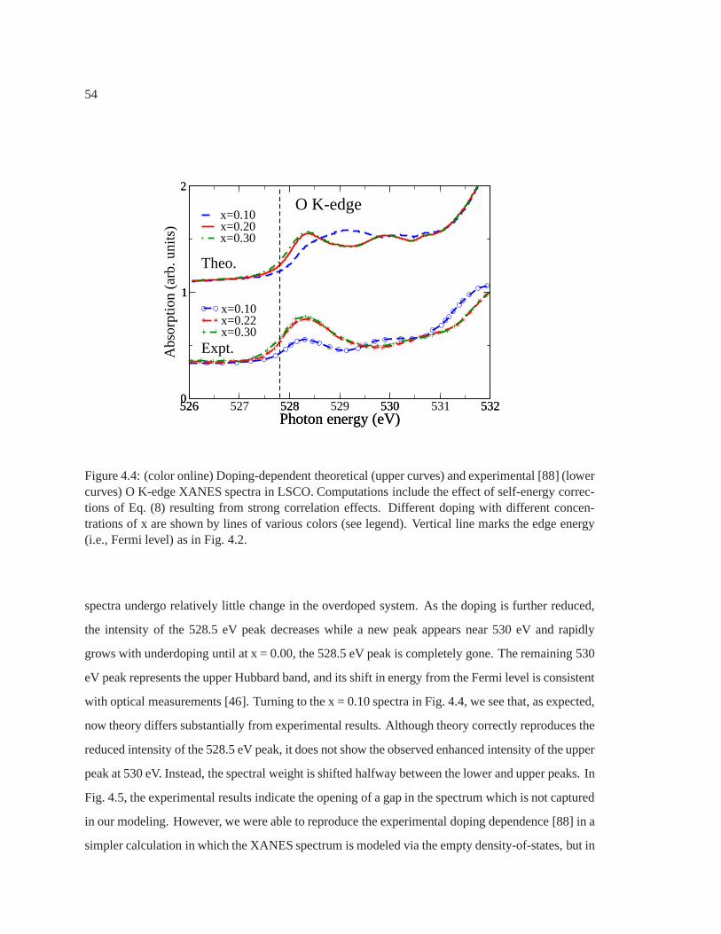
54
526 527 528 529 530 531 532Photon energy (eV)
0
1
2
x=0.10x=0.20x=0.30
526 528 530 532Photon energy (eV)
0
1
2A
bsor
ptio
n (a
rb. u
nits
)
x=0.10x=0.22x=0.30
Expt.
Theo.
O K-edge
Figure 4.4: (color online) Doping-dependent theoretical (upper curves) and experimental [88] (lowercurves) O K-edge XANES spectra in LSCO. Computations include the effect of self-energy correc-tions of Eq. (8) resulting from strong correlation effects.Different doping with different concen-trations of x are shown by lines of various colors (see legend). Vertical line marks the edge energy(i.e., Fermi level) as in Fig. 4.2.
spectra undergo relatively little change in the overdoped system. As the doping is further reduced,
the intensity of the 528.5 eV peak decreases while a new peak appears near 530 eV and rapidly
grows with underdoping until at x = 0.00, the 528.5 eV peak is completely gone. The remaining 530
eV peak represents the upper Hubbard band, and its shift in energy from the Fermi level is consistent
with optical measurements [46]. Turning to the x = 0.10 spectra in Fig. 4.4, we see that, as expected,
now theory differs substantially from experimental results. Although theory correctly reproduces the
reduced intensity of the 528.5 eV peak, it does not show the observed enhanced intensity of the upper
peak at 530 eV. Instead, the spectral weight is shifted halfway between the lower and upper peaks. In
Fig. 4.5, the experimental results indicate the opening of agap in the spectrum which is not captured
in our modeling. However, we were able to reproduce the experimental doping dependence [88] in a
simpler calculation in which the XANES spectrum is modeled via the empty density-of-states, but in

55
527 528 529 530 531Photon energy (eV)
0
1
2
3
4
Abs
orpt
ion
(arb
. uni
ts)
O p-DOS x=0.00O p-DOS x=0.10Expt. x=0.00Expt. x=0.10
Theo. (DOS)
Expt.(XANES)
O K-edge
Figure 4.5: (color online) O K-edge XANES from experiment [101] (lower set of broken curves)for x = 0.00 and x = 0.10, compared with theoretical single-band p-DOS (upper curves) for Opl forx = 0.00 and x = 0.10 [89]. The vertical line marks the edge energy (i.e., Fermi level) as in Fig. 4.4.
which self-energy corrections including the magnetic gap are incorporated [89]. Fig. 4.5 compares
the experimental XANES spectrum with this DOS approximation at x = 0.10. The splitting of
the spectrum into two peaks with the appropriate gap is well reproduced. It should be noted that
this same self energy reproduced the optical and RIXS gaps asa function of doping [46, 90, 92].
Interestingly, the good agreement between theory and experiment in the overdoped case implies that
the upper peak at 530 eV possesses little weight in the overdoped system. In particular, we find a
saturation of the lower energy feature ( 528eV) in the O K-edge spectra [Fig. 4.4] as the doping
value is increased beyond the optimal doping, except for theFermi edge shift. This saturation is in
good agreement with the experiment by Peetset al. [88], but is inconsistent with model calculations
by Liebsch[102] and Wanget al. [103]. This effect requires a transfer of spectral weight from the
upper to the lower peak, which is much larger than that predicted byt-J models of the cuprates [89].
A similar conclusion was arrived at by Peetset al. [88]. Such anomalous spectral weight transfer

56
has been discussed in several spectroscopies of cuprates [46, 104, 105]. The present intermediate
coupling calculations can provide a satisfactory explanation of these results.
4.5 Conclusion
We have carried out a realistic calculation of the XANES of the cuprate superconductor LSCO. Our
focus in this first such attempt is on the O K-edge XANES in overdoped LSCO over the hole doping
range x = 0.20 to x = 0.30. For this purpose, we have incorporated doping dependent self-energy
corrections due to strong electron correlations into a realspace Green’s function formalism, which
is implemented in the FEFF9 code. Good agreement is found between theoretical and experimental
doping evolution of the XANES in overdoped LSCO. Although LSCO has two chemically distinct
O-atoms, the O K-edge XANES is dominated by the contributionof O-atoms in the cuprate planes.
Apical O-atoms only begin to make a significant contributionto the spectrum at higher energies,
>531 eV. In examining effects of the core-hole screening, we find that the spectra are insensitive to
the core-hole screening model at least in the overdoped regime. In the underdoped case, as expected,
our self-energy corrections, which are appropriate for theoverdoped paramagnetic system, fail to
correctly describe salient features of the spectra. A simple calculation suggests that correcting this
will require a more comprehensive modeling of XANES including effects of pseudogap physics on
the self-energies in the underdoped regime.

57
Chapter 5
CHARGE TRANSFER SATELLITES IN STRONGLY CORRELATED SYSTEMS
Many strongly correlated systems such as transition and rare-earth compounds, chemisorption
systems, and high-Tc compounds have charge transfer or ‘shake-down’ between themore localized
outer level (d) and less localized level (L). Following a three electron level model prescribed by Lee
et al. [20] a perturbative construction of a spectral function is described in this chapter. Our real-
space multiple scattering calculation for the Cu K-edge XANES of La2−xCuO4 and Nd2−xCuO4
was compared with the experimental result by Kosugiet al. [21]. A convolution of our calculated
XANES with the Lee-Hedin spectral function took the missingmany-body charge transfer effects
into account, and was found to be in good accord with experiment.
5.0.1 Outline of this chapter
In this chapter we summarize the perturbative approach proposed by Leeet al. [20] to get the charge
transfer satellites in Cu compounds. Section 5.2 discussesa short introduction of the nature of this
problem, while section 5.3 is dedicated to our summary of theperturbative technique prescribed in
the PRB paper by Lee and Hedin [20]. In section 5.4 we discuss our prescription of constructing a
charge-transfer spectral function using the ‘main peak to satellite’ ratio from Leeal. We apply this
spectral function in our RSGF calculation for Cu K-edge in LSCO and NCCO in section 5.5.
5.0.2 Key observation
Our RSGF calculated Cu K XANES convoluted with the charge-transfer spectral function gives
good agreement with the experiment by reproducing the satellites in LSCO and NCCO.
5.1 Introduction
For many strongly correlated systems the core-level spectroscopy is effected by collective excita-
tions and show satellite like features such as ‘shake-down’or ‘shake-up’. For example Cu com-

58
pounds often show such features. In one of the early experiments, Kosugiet al. [21] measured
such satellites in the Cu K-edge XANES of NCCO and LSCO and identified them as the ligand-
to-metal charge transfer satellites (LMCT). In the ground state, Cu has 3d9 configuration while all
the ligand orbitals are filled. In the core-level x-ray experiment a core-hole in Cu can be created
and it becomes energetically favorable for an electron to transfer from the ligand (4s) to the Cu site
ending with 3d10 configuration. In the latter case the core-hole will be strongly screened. Due to
hybridization between thed9 andd10 configurations, the final states will be a mixture of the two
configurations as indicated in Fig. 5.1. In the sudden approximation limit, when the photo-electron
kinetic energy is high and extrinsic and intrinsic losses decouple, this satellite feature caused by
the screening strength of the two configurations is usually observed in the photo-emission experi-
ments. Within the sudden approximation one can then construct a spectral function by extracting
two parameters from the photo-emission spectrum which are the the ratio of the peak intensityr0(ω)
and energy splitδE between the main and the satellite peak. About 10 eV above theedge energy,
such satellites were also observed in some of the Cu K-edge XANES of the high-Tc cuprates. But
obtaining a spectral function for such spectrum is not straightforward since this energy range falls
within the adiabatic limit where the extrinsic and intrinsic losses don’t decouple. In this chapter we
closely follow the three electron model prescribed by Lee and Hedin [11] where we consideredr00
(= r0(ω)|ω→∞), andδE as parameters.
5.2 Lee-Hedin charge transfer satellite model
The Lee-Hedin model as proposed by Leeet al. [20] is a three electronic level model that starts with
a Hamiltonian,
H0 = εana + εLnL + εcnc +Uancna +Ubncnb + t(c†acL +c†
Lca). (5.1)
The first two terms give the eigenvalues of the localized state (e.g. 3d) and delocalized ligand state
L. The last term is the hybridization between them. The remaining terms give the energy(εc) and
occupation(nc) of the core state. In x-ray absorption or photoemission spectroscopy, a core electron
is excited leaving behind an empty core statec. Sonc = 1→ 0. In Cu compounds, for example,c
may represent the Cu 1s core level,a the localized Cu 3d valence level andL a ligand state (e.g.,
hybridized state between Cu 4s and O 2p). With x-ray excitation the total Hamiltonian can be

59
1
Strong
Screening
3d104s1
Weak
Screening
3d94s2
Initial Final
(main)
Final
(Satellite)
4s 4s 4s 3d
3d 3d
core hole core hole core
3 4 4 3( )DFTi i ij d s s di j
i ij
H n U n n t c c c cV VV
Hn p
¦ ¦
LDA+U Ligand Æmetal
charge transfer
Figure 5.1: Spectral function of the electron-doped high Tc cuprate Nd2−xCexCuO4 using the sepa-rable potential approach of Lee-Hedin model
written as,
H = H0+T +V + ∆. (5.2)
HereT is the sum of one-electron kinetic energies of continuum state,
T = ∑k
εknk (5.3)
with energiesεk = k2/2, and wave functionsψk obtained from a one-electron potential in the pres-
ence of core-hole (nc = 0). The perturbation causing photoemission is
∆ = ∑kc
(Mkc†kcc +h.c.), (5.4)
whereMk is the transition matrix element. Now the interaction between the photo-electrons are
taken as,
V = ∑kk ′
[naV(a)kk ′ +nbV
(b)kk ′ −V(c)
kk ′ ]c†kck′ . (5.5)

60
HereVkk ′ is a matrix element of the Coulomb potentialV(ν)(r) from the charge density of the orbital
ν
Vνkk ′ =
Z
ψ∗k(r)
ρν(r ′)|r − r ′|
ψk′(r)drdr ′ (5.6)
To obtain charge transfer satellites these matrix elementsMk andVkk ′ can in principle be cal-
culated using the real-space multiple scattering code FEFF. But in this chapter we take a simplistic
approach to calculate the spectral function and closely follow the prescription by Leeet al. [20].
In their model with three electron levels the valence wave functions were calculated using muffin
tin potentials with radiusR, and then the calculated matrix elements were fitted to get ananalytical
expression forMk andVkk ′ .
Mk =εk/Ed
1+ εk/Ed, (5.7)
whereεk = k2/2, Ed = 1/2R2d, and for 1score stateRd is a length scale taken asRdx≈ 0.5 a.u. And,
Vkk′ =VRs
R1
1+R2sd(k−k′)2
. (5.8)
HereRs is the length scale of the interactionVkk ′ andRs = 1.77 a.u., andR is the muffin tin radius.
More detail of these derivations can be found in [20].
5.2.1 Three Level System without interaction, V= 0:
Initially when nc = 1, the ground state ofH0 is given by
|Ψ0〉 = −sinθ |ψc〉 |ψa〉+cosθ |ψc〉 |ψL〉 , (5.9)
with eigen energy,
E0 = εc +12(εa +U + εL)−
12
√
(εa +U − εL)+4t2, (5.10)
where
tan2θ =2t
(εa +U − εL). (5.11)
In the final state whennc = 0, the two possible states (due to charge transfer between ligand and
3d states) are
|ψ1〉 =cosφ |ψa〉−sinφ |ψL〉
|ψ2〉 =sinφ |ψa〉+cosφ |ψL〉 , (5.12)

61
with eigenenergies
E12 =
12(εa + εL)∓
12
√
(εa− εL)2 +4t2, (5.13)
and
tan2φ =2t
(εL − εa). (5.14)
HereδE can be defined as the energy separation between the main and satellite peaks,
δE =√
(εa− εL)+4t2. (5.15)
The photocurrents for main(s=1) and satellite(s=2) are given [20] by
Jsk(ω) =
∣
∣
∣
⟨
Ψskf
∣
∣∆ |Ψ0〉∣
∣
∣
2δ(ω− εk +E0−Es), (5.16)
where∣
∣
∣Ψsk
f
⟩
is a final state. In the sudden approximation the final state can be written as∣
∣
∣Ψsk
f
⟩
=
|ψs〉 |ψk〉. Now, summing overk one obtains absorption spectraJs(ω),
Js(ω) = ∑k
Jsk(ω). (5.17)
In the sudden approximation, the kinetic energy of photoelectrons is large, and we can take
k1 = k2. The ratior00 of the satellite to the main peak intensity then is,
r00 = limω→∞J2(ω)
J1(ω)= cot2(φ+ θ). (5.18)
Taking the k dependence ofMk we obtain,
r0(ω) = r00
[
∆ω∆ω+ δE
]
×
[
1+(∆ω+ δE)/Ed
1+ ∆ω/Ed
]
Θ(∆ω). (5.19)
Here∆ω = ω = ωth andωth = E2−E0. From Eqs.5.13 to 5.19 we see thatr00 andδE equivalently
describes the two parametersU andt used by Lee-Hedin model. In this chapter, these are the two
parameters we used to construct the spectral function in order to convolute the absorption spectra
obtained from FEFF code for the case of Cu K-edge in LSCO and NCCO.
5.2.2 Three Level System with interaction, V6= 0
Now turning on the interaction between the photoelectrons in the continuum state the Hamiltonian
is,
H = H0+T +V. (5.20)

62
The exact, final photoelectron state is
∣
∣Ψskf
⟩
=
[
1+1
E−H0−T −V − iηV
]
|ψs〉 |ψk〉 , (5.21)
where|ψs〉 (s=1,2) are the eigenstates ofH0 with the core-hole, andE = εk +Es is the energy of the
final state. Now, the dipole transition matrix elementM(s,k) =⟨
Ψskf
∣
∣
∣∆ |Ψ0〉 can be written as
M(s,k) = 〈ψk| 〈ψs|
[
1+V1
εk +Es−H0−T −V + iη
]
∆ |ΨO〉 . (5.22)
At this point instead of exact treatments we will use the firstorder perturbation inVkk′ to obtain
the transition matrix elements as prescribed by Leeet al. To the lowest order inV one ignores the
V term in the denominator of Eq .5.22. Inserting the completeness relation∑i |i〉〈i| in terms of the
eigenstate|i〉 = |k〉 |s〉 we obtain
M(s,k) = 〈s| 〈k|∆ |Ψ0〉+∑k′s′
Vks,k′s′ [(E−H0−T + iη)−1]k′s′,k′s′⟨
s′∣
∣
⟨
k′∣
∣∆〈Ψ0〉 . (5.23)
Fors= 1,2 one obtains
M(1,k) = −sin(φ+ θ)Mk−sin2 φ sin(φ+ θ)∑k′
[
Vkk′Mk′
E−E1− εk′ + iη
]
−sin2φ cos(φ+ θ)
2 ∑k′
[
Vkk′Mk′
E−E2− εk′ + iη
]
, (5.24)
and
M(2,k) = cos(φ+ θ)Mk +cos2 φ cos(φ+ θ)∑k′
[
Vkk′Mk′
E−E2− εk′ + iη
]
+sin2φ sin(φ+ θ)
2 ∑k′
[
Vkk′Mk′
E−E1− εk′ + iη
]
. (5.25)
In the above two equations we used
Vi j = Vks,k′s′ = Vkk′vsvs′ (5.26)
wherevs = −sinφ if s= 1, andvs = cosφ if s= 2.
Now consideringRk = Rs = R, Leeet al. [20] defined a functionFk by
∑k′
Vkk′mk′
ε− εk′ + iη= −
VE
MkFk(ε/E), (5.27)

63
using the simple analytical form ofVkk′ andMk from Eq .5.7 and Eq .5.8. Thus,
Fk(ε) =1π
Z ∞
0
x4dx
[1+x2]2 [1+(Rk−x)]2 [x2− ε− iη]. (5.28)
From Eq.5.24 and Eq.5.25 one obtains
r(ω)
r0(ω)=
∣
∣
∣
∣
∣
∣
1−cos2φ VE Fk2(
ωE )− sin2φ sin(φ+θ)
2cos(φ+θ)VE Fk2(
ω+δEE )
1−sin2φ VE Fk1(
ω+δEE )− sin2φ cos(φ+θ)
2sin(φ+θ)VEFk1(
ωE )
∣
∣
∣
∣
∣
∣
2
, (5.29)
wherer/r0 depends only onV/E, δE/E, and∆ω/E. Using the above equation along with Eqs.5.18
and 5.19 we getr(ω) and finally construct the charge transfer spectral function.
5.3 Spectral function
In order to construct the spectral function to account for charge transfer effects we start with a
spectral function of the following form,
A(∆ω) = C1(∆ω)δ(∆ω)+C2(∆ω−δE). (5.30)
For notational simplicity and to avoid confusion, from hereon we will denote∆ω = ω. Now the
coefficients of the normalized spectral function
A(ω) = C1(ω)δ(ω)+C2(ω−δE) (5.31)
has the following two conditions;
C1(ω)+C2(ω) = 1
C1(ω)
C2(ω)= r(ω). (5.32)
Here we usedδE andr00 as parameters which are equivalent and obtainable fromt andU used in
the Lee-Hedin model. Such spectral functions can be used to convolute the calculated spectra to
account for the charge transfer effects.
µ(ω) = µFEFF(ω,ω′)∗A(ω′) (5.33)
For high-Tc Nd2−xCuO4 we usedδE ∼ 8 eV from the satellite peak position in Cu K-edge XANES
experiments andr00 = 2.3 is taken as the best fitted value.

64
oÚ:Ó)
oÛ:Ó;
Ó
Ó
r:Ó) = oÚ:Ó;
oÛ:Ó;
Figure 5.2: Spectral function of the electron doped high Tc cuprate Nd2−xCexCuO4 using the sepa-rable potential approach of Lee and Hedin model
5.4 X-ray spectroscopy of High Tc materials
Both in NCCO and LSCO, Cu K-edge XANES show the remarkable satellite feature 7 or 8 eV apart
from the main peak. We see the presence of such peaks in the experiment (dashed green) curve of
Figs. 5.4 and Fig.?? at 22 eV, and again at around 38 eV.
We calculated the Cu K-edge XANES using the real-space multiple scattering code FEFF (solid
red curve) and (see in Fig. 5.4 and Fig.??). Being a single configuration code, FEFF fails to
account for any charge transfer effects and misses the satellite structure. Significant improvement
was achieved by convoluting the FEFF calculated spectra with the spectral function obtained from
the Lee and Hedin model. The post-convoluted XANES is plotted in the solid blue curve in Fig. 5.4
and Fig.??. For LSCO in Fig. 5.4 we see a shoulder like feature at 22 eV before the convolution
which is caused by the structure of the system mainly due the presence of the apical oxygen atoms.
This feature is completely absent in the spectrum of NCCO in Fig. ?? (solid red line) which does

65
0 20 40 60 80Photo-electron Energy (eV)
0.0
0.5
1.0
1.5
2.0
Abs
orpt
ion
(Arb
itrar
y U
nit)
FEFF FEFF with Satellites (Lee-Hedin Model)Experiment (Kosugi et al.)
Cu K-edge XANES in LSCO
Figure 5.3: Cu K-Edge XANES of La2−xSrxCuO4 with and without charge transfer satellite correc-tion
not have any apical oxygen. We have confirmed this by calculating the spectrum of structures with
longer distance between the apical oxygen atoms and Cu in LSCO which tends to wash this peak
out at 22eV. Spectral convolution enhances the satellite peaks for both these materials.
5.5 Conclusion
Following Lee and Hedin’s three level model and using two parameters extracted from experiment
we have constructed a spectral function which in principle can account for the charge transfer from
delocalized to localized orbitals in correlated systems. FEFF calculated XANES convoluted with
this spectral function correctly reproduce the charge transfer satellites observed in the Cu K-edge
XANES of high-Tc cuprates Nd2CuO4 and La2CuO4 [21]. The construction of the spectral function
employed the analytical formulation of potential and dipole transition matrix elements as prescribed
by Leeet al. [20]. Although this simple formalism improves the spectralfeatures significantly, a

66
0 10 20 30 40 50 60 70Photo-electron energy (eV)
0.0
0.5
1.0
1.5
2.0
2.5A
bsor
ptio
n (A
rb. U
nits
)FEFFFEFF with Satellites (Lee-Hedin model)Experiment (Kosugi et al.)
Cu K-edge XANES in Nd(2-x)
CexCuO
4
Convoluted with A(ω)
A(ω)=Z δ(ω) + (1-Z) δ(ω − ωsat
)
1-Z(∆ω) = r(∆ω) ; ωsat
~ 7 eV
Figure 5.4: Cu K-Edge XANES of Nd2−xCexCuO4 with and without our charge transfer satellitecorrection
more robust calculation ofVkk′ andMk can be done within the real-space multiple-scattering frame-
work is in progress.

67
Chapter 6
OTHER ELECTRONIC STRUCTURES: DNA-GRAPHENE HYBRIDS
We calculate the electronic local density of states (LDOS) of DNA nucleotide bases (A,C,G,T)
deposited on graphene. We observe significant base-dependent features in the LDOS in an energy
range within a few eV of the Fermi level. These features can serve as electronic fingerprints for
the identification of individual bases in scanning tunneling spectroscopy (STS) experiments that
perform image and site dependent spectroscopy on biomolecules. Thus fingerprinting of DNA-
graphene hybrid structures using STS may provide an alternative route to DNA sequencing.
Additionally we calculate the conductance current throughGraphene nano ribbon with DNA
nucleotide bases (A,C,G,T) inside a pore. We observe significant base-dependent features in the
transmission and its first derivative in an energy range within a few eV of the Fermi level. These
features can serve as electronic fingerprints for the identification of individual bases in nano-pore ex-
periments in vacuum. Thus the fingerprints of DNA in graphenenano-pore may provide a guideline
and alternative route to DNA sequencing.
6.1 Electronic Fingerprints of DNA bases on Graphene
The determination of the precise sequences of the four nucleotides [adenine (A), cytosine (C), gua-
nine (G) and thymine(T)] in DNA molecules is an important goal for both fundamental research
interests as well as a large number of applications in biomedical research [106], bio-technology
[107, 108], drug delivery [109], and biomaterial growth [110]. However, conventional approaches
are generally complex and expensive [111]. Numerous experimental and theoretical [112–114]
attempts have been made to improve such determinations. Forexample, efforts have been made
to develop efficient techniques based on high-resolution microscopic [115, 116] and spectroscopic
[117] probes that can yield direct fingerprints of these biomolecules. However, these techniques
require the biomolecules to be deposited on a host substratein an ultra-high vacuum environment.
Difficulties in preparing high-quality samples and in obtaining reproducible measurements have lim-

68
ited the utility of these approaches [118]. For example, theelectronic fingerprints of a given DNA
base can vary dramatically even for subtle changes in the relative angle of a base with respect the
substrate [119]. On the other hand, a recent scanning tunneling microscopy/spectroscopy (STM/S)
study [117] by Tanakaet al. has shown that the guanine base of DNA on a Cu(111) surface always
exhibits a strong tunneling peak around a fixed bias voltage of -1.6 eV, thus providing a reliable
marker in tunneling measurements. This observation has ledto a significant advance in the field,
since it opens an opportunity for electronic identifications of all bases via tunneling conductance
from a local probe. However, the localizedd states and the dangling bonds near the surface of the
bulk Cu are among the many effects that can complicate the implementation of this approach, thus
suggesting the importance of finding a more suitable substrate.
STM experiment Pos. bias maps Unoccu. states Neg. bias maps Occu. states
a b c Figure 6.1: a Schematicillustration of STM experi-ment which can extract to-pographical image and dI/dVinformation of a sample ly-ing on graphene plane;b andc schematically demonstratetunneling between the tip andsample. Based on positive(b) or negative (c) bias volt-age, electrons can transmit toor from the graphene and mapthe unoccupied or occupied lo-cal density of states (LDOS)correspondingly of the samplelying on the plane.
We show that an attractive substrate to consider is graphene, a purely two-dimensional sheet
of carbon atoms arranged in a honeycomb lattice [120]. Amongits unique properties, graphene
possesses linearly dispersed Dirac quasiparticles with a semimetal density of states near the Fermi
level [120, 121]. Additionally, graphene combines a conducting surface with remarkable mechani-
cal strength. Also strongπ−π interactions between DNA bases and conjugated carbons in graphene
should favor mostly plane orientations of DNA bases with respect to the surface [122] and, thus, re-
sults in relatively homogenous orientations of bases in theDNA strands when it adsorbs on graphene

69
and offers optimal conditions for STM measurements. These characteristics make this novel ma-
terial an excellent surface for studying adsorbates of various organic macro-molecules. Several
successful implementations of graphene have already been reported recently in electronic devices
and biomedical and bioassay applications [123–125]. We aimto develop a detailed understanding of
the interaction and adsorption between graphene and biomolecules such as the DNA bases including
local electronic structure, using an approach that goes beyond the structural analysis of such hybrid
systems.
To achieve this goal, we have carried out extensive DFT-based, first-principles, numerical simu-
lations of the electronic local densities of states (LDOS) of all four DNA bases on graphene. Con-
sidering only the short range interaction between the DNA bases and graphene, the van der Waals
interaction was not included in our calculation. It was previously demonstrated that on distances
of 2 to 3A, the long range dispersion interaction correction becomes negligible [119, 126, 127].
We find that the electronic LDOS of the nitrogen atom can serveas an electronic fingerprint of a
particular DNA base. That is, we find several distinguishingand dominant features in the LDOS
that can identify each base. This finding can be used in conjunction with STM/S measurements of
atomic resolution that image and probe the local density of states(LDOS) of surfaces, as illustrated
in Fig. 6.1. In particular, i) we deduce that the local chemical environment and the graphene base
leads to new electronic states and additional features in the local density of state (LDOS) inside
the parent highest occupied molecular orbital (HOMO) and lowest unoccupied molecular orbital
(LUMO) insulating gap. ii) For each base the peak positions and peak heights exhibit a charac-
teristic evolution as a function of their orientation with respect to the graphene sheet; iii) We also
investigate the similarities and differences of the LDOS ofDNA bases by placing the graphene on
the commonly used SiC substrate. The STM topography simulations also add important insights
into the characterization of charge distributions and hybridization of states between bases as well
between base and graphene. Taken together, we demonstrate that all four bases of DNA adsorbed on
a graphene substrate can be differentiated quantitatively. This suggests the possibility of an efficient
and cost-effective sequencing approach.
In an STS experiment, measurements are done in two steps. First, the tip scans over the surface
to search for the locations of the maximum transmission currents at a fixed voltage (6.1(a)) and
constructs the topographic image. In the next step, the voltage is varied over an energy range

70
Figure 6.2: (a) Molecu-lar energy levels of each iso-lated DNA base molecule;(b)Upper panel shows LDOS ofcarbon atom in pure grapheneand lower panel shows nitro-gen peak LDOS in isolatedDNA bases. (c) Integrated( -3.0 eV to EF = 0) partialcharge density of DNA baseson graphene plane. Base typesare organized in columns andangles between base-ring andgraphene plane are variedalong rows as indicated. Thissimulation of STM topogra-phy is done using HIVE-STM[128] code.(d) Molecular ori-entations of DNA bases corre-sponding to the images inc aredisplayed.
by keeping the tip position fixed, and the differential current dI/dV which determines the local
electronic structure (LDOS) of the sample is then measured.A schematic illustration is presented
in 6.1(b) and (c).
We first considered the behavior of isolated DNA base molecules using DFT calculations. In
6.2(a), the molecular energy levels of each base are reproduced, in agreement with previous calcu-
lations [119]. These results confirm that all nucleo-bases have a large HOMO-LUMO gap (Eg ≈
5 eV). Near the energy gap, all electronic features are qualitatively similar for all four bases. Such
small variations in the electronic structure of DNA bases might bring in to question whether STM
is able to resolve fingerprints features of DNA bases. On the other hand, the presence of a sub-
strate and subsequent interactions significantly affect the alignment of electronic levels of bases
compared to the isolated molecules as was theoretically predicted for adsorbed DNA bases on the
Cu surface [119]. We have considered an experimental setup with freeze-dried conditions, that will
result in significantly diminished noise due to the changes of molecular configuration and due to
low temperature.
To investigate the effect of graphene on the DNA bases, we first calculate the LDOS of nitrogen

71
Figure 6.3: a Solid linesare nitrogen LDOS in ade-nine adsorbed on graphenewith different angles, and theshaded regions show the dom-inant peak features near EF
on both positive and nega-tive energy side, 0 eV cor-responds to Fermi energy;b,c, andd shows similar LDOScurves for cytosine, guanineand thymine correspondingly;e Dominant peak positionsnear EF for different anglesand bases. Positions of thepeaks are plotted along y-axisand angles along x-axis. Therelative size of the symbols re-flects the relative peak inten-sity for each case.
atoms in the isolated DNA bases and the LDOS of carbon atoms inthe bare graphene as shown
in 6.2(b). For the bare graphene, our calculation reproduces the well-known and distinct electronic
feature of graphene at EF – the presence of a Dirac cone [129] – as can be seen in 6.2(b).
STM topographical images also provide important geometricinformation. This is particularly
important in systems where molecules of interest can interact with the surface at many different
orientations. Depending on the backbone configuration, DNAbases in a single stranded (ssDNA)
can be adsorbed onto the graphene surface at different angular orientations and further complicate
the electronic identification. Thus, we constructed supercells where each DNA base lies on the
graphene surface with four possible angles (6.2(d)). In order to simulate a STM topographic image
theoretically, we integrated our DFT based partial charge density from -3.0 eV to EF using HIVE-
STM [128] (6.2(c)). The average distance between the DNA bases and graphene plane was fixed at
3.0A.
In the remainder of this study, we primarily focus on the dI/dV (or LDOS) of DNA bases on
graphene. Since nitrogen is a common constituent of all fourbases with the most diffuse orbitals,
we analyze the dependence of the LDOS on both the DNA base and its spacial orientation when a

72
featureless tip is placed directly above a nitrogen atom. The calculated LDOS is shown for isolated
DNA bases (6.2(b)) and adsorbed bases (6.3). For the adsorbed bases, we identify the behavior of
the dominant peak features within the range of -3.0 to 3.0 eV,and their dependence on the angle
between the base-ring plane and graphene plane. These peaksare marked by the colored shaded
regions in the curves of 6.3(a)-(d). In 6.3(e), we summarizethese angle dependent results for the
positive and negative bias energies for all four bases.
By examining 6.3, one can recognize the dominant STS peak features, except for a few cases
where the experimental resolution can play a critical role.For example, simulated LDOS (6.3(e))
shows distinctive features in the positive low energy region (unoccupied states) for cytosine (the
lowest among all) and guanine (the highest among all), independent of the base orientation.
Consequently, if several LDOS peaks are compared (for example, both occupied and unoccupied
states close to the Fermi energy), the identification of the bases can be achieved. For the above
example the supercell consisted of a set of∼ 130 atoms, and a full geometry optimization on such
systems is computationally expensive. To asses the interaction between the graphene and the bases,
we reduced the supercell and performed a full geometry optimization using VASP [14, 130, 131]
software package.
Our calculations reveal the dependence of the binding energies on the angular orientation for
a given base. For example, the 0 configuration of adenine is more bound than the 45 one. The
preference in plane alignments of bases with respect to the graphene is expected, since parallel ori-
entation of bases along the graphene surface allows better overlap inπ orbitals between the aromatic
rings of DNA bases and aromatic carbons in graphene increasing theπ−π stacking. This interac-
tion results in relatively homogeneous and planar orientations of bases in the DNA strand adsorbed
on the graphene, which offers favorable conditions for STM experiment and better resolution of
dI/dV features. At small angles (<15 degrees), the highest occupied states of cytosine and guanine
(below Fermi energy) are well distinct from adenine and thymine, as can be seen in 6.3(e). In addi-
tion, at plane configurations, the peaks corresponding to the highest occupied states of adenine and
thymine have closely lying satellite peaks, while guanine and cytosine have well-separated sharp
peaks. Thus, comparing several peaks (occupied and unoccupied) and their shapes will provide
necessary fingerprints to differentiate DNA bases.
In STM experiments, graphene is often supported by another substrate, such as silicon carbide.

73
Figure 6.4: a Super-cell that includes single lay-ered SiC crystal under the2D graphene plane. b ni-trogen LDOS of four DNAbases (adenine (black), cyto-sine (red), guanine (green),and thymine (blue). Solidlines are for the bases ad-sorbed on graphene+SiC sub-strate; the dashed lines are thenitrogen LDOS for isolatedbases. The LDOS curve forthe nearest neighbor Si atomis displayed in orange solidcurve, and the topmost curveis for carbon LDOS in puregraphene. The shaded colored(blue) regions are the domi-nant peak positions due to hy-bridization between N and C(graphene) atoms, and shadeddark regions are due to hy-bridization between N and un-derlying nearest Si atom.
To better simulate real systems we added a single layered silicon carbide (SiC) crystal under the
graphene sheet. Fig. 6.4 presents our calculated nitrogen LDOS for each base, where the base-ring
plane and graphene plane are parallel to each other. The LDOSof the Si atom nearest to the base
molecules is shown by the orange solid line in 6.4. Surprisingly, the orbitals of the DNA bases
are spread over the SiC despite the separating layer of graphene. Such a ”see through effect” is
pronounced for Si states close to EF resulting in the hybridized peaks of nitrogen LDOS indicated
by the black shaded regions.
We see this effect only in close proximity to EF , and the STS resolvable dominant features
around ± 2.0 eV remain identifiable. These latter peaks originate from the hybridized states be-
tween the DNA bases and graphene and are shown by the blue shaded regions in 6.4. The dominate
peak features near 1.0-2.0 eV are well-pronounced for guanine and adenine. The largest peak fea-
tures of adenine and guanine at 2.0-2.5 eV also have potential as electronic fingerprints for STS

74
experiment.
6.2 Identifying DNA bases with Transport Current
A major goal in medical research is to develop a fast, accurate and low cost DNA sequencing tech-
nique that can sequence a diploid mammalian genome for $1000within 24 hours. The nanopore-
based devices provide a highly confined space that can identify the presence of a single DNA nu-
cleotide passing through the pore using a variety of ways of creating identifiable signals [132]. Some
of the recent table top experiments [133] show promising andpotentially useful results using pro-
tein nanopores. But none of these methods are error free due to high noise to signal ratio in the ion
channeling method through complex pores.
In this section we propose a simple nanopore device constructed with a punctured graphene
mono-layer ribbon which is suspended between two gold electrodes. We use 2 eV bias voltage
between the electrodes. Using DFT and NEGF techniques implemented in ‘TranSiesta’ version of
the code ‘SIESTA’ [134, 135], we calculate the transmissioncurrent between the electrodes, while
placing Adenine (A), Guanine (G), Cytosine (C), and Thymine(T) inside the pore. This simple
device geometry is schematically shown in Fig. 6.5
Figure 6.5: Schematicillustration of nano-poreexperiment which can extractdI/dV information of a samplepassing through the graphenenano-pore; a Adenine, bCytosine c Guanine, andd Thymine; Based on thepositive (b) or negative(c) bias voltage betweenthe electrodes, electronscan transport through thegraphene nano-ribbon , andmap the conductance of thesample lying inside the pore.
Our calculations are limited to identifying only the singlenucleotides one at a time, and ignoring

75
the phosphate back-bone structure of sDNA. Assuming the back bone will only contribute to a
consistent shift in the transmission signal, we here focus on the detection of distinct features in the
transmission current due to different isolated DNA bases inside the pore.
Figure 6.6: Differencecurve of the average conduc-tance of isolated DNA basesinside nanopore. Average istaken over angular configura-tion. (a) Adenine, (b) Cy-tosine, (c) Guanine, and(d)Thymine. The fermi energy isat 0 eV and difference curveshows distinguishing featuresfor each of the DNA bases.the solid curve on each dif-ference curve shows the inte-grated conductance or current.
In our calculation we have taken random angular orientationof the isolated bases inside the pore,
and calculate the average transmission. The transmissiondI/dV and its first derivatived2I/dV2
show identifiable features near zero volt for each of these bases as shown in Fig. 6.6 and Fig. 6.7.
Fig. 6.6 shows the differential curves between A, C, G, and T.
Our calculations are carried out for the configuration averaged transmission currents and their
derivatives with respect to the voltage. This is in contrastwith the flat orientation of DNA nu-
cleotides inside the pore as reported by Nelsonet al. [136]. Here we take the diameter of the
punctured hole on graphene as 15A, and the carbon atoms inside the pore are not capped with
Hydrogen. Hydrogen capping and the size of the nanpores can affect signal significantly, and thus
call for a more systematic study. As we see in Fig. 6.6, our theoretical results are not completely
free from noise. The proposal for better noise reduction techniques along with a more convenient
device geometry is currently under progress and will be carried as a future direction of this project.

76
Figure 6.7: Average conduc-tancedI/dV (solid red) andd2I/dV2 (solid green) ofaAdenine,a Cytosine,a Gua-nine, anda Thymine througha graphene nanopore. Ver-tical dashed line is at theFermi energy at 0 eV. Dom-inant features near Fermi en-ergy in d2/dV2 distinguishesDNA bases passing throughthe nano-pore.
6.3 Conclusion
In conclusion, we propose the use of graphene as a depositionsubstrate for macromolecular se-
quencing. Both the Dirac linear dispersion of electronic states in graphene and its robust mechanical
properties serve to make it a superior substrate compared tometals. We have calculated the tunnel-
ing conductance and LDOS for the specific case of single DNA bases at various orientations on
the surface, and shown that the different nucleotides have significantly different LDOS peaks (fin-
gerprints), allowing differentiation via local tunnelingconductance. The calculated nitrogen atom
LDOS for A,T,C, and G bases show distinct peaks that vary depending on configuration. We find
that Guanine provides the largest peak at a negative bias at -1.3 eV, i.e., a slightly higher energy than
guanine on copper [117]. Nonetheless, peaks for the other bases at higher energies have features
at positive and negative STM bias, and provide fingerprints that allow unique identification. The
calculated LDOS fingerprints can help guide STS as an approach to identify DNA bases, and likely
other biomolecules on graphene surfaces.

77
Chapter 7
CONCLUSION
Studying the x-ray spectroscopy of correlated systems within RSGF framework and Hubbard
model has been the primary focus of this thesis. Three different developments in this direction are
discussed in chapters 3, 4, and 5. Many spectral features near the Fermi energy call for theoretical
development beyond the single particle approximation. This is equally true for the conventional
DFT and Green’s function based approaches. To achieve a computationally cheap and efficient
scheme, one often relies on some combination of model Hamiltonian and first-principle approaches.
Chapter 3 is primarily dedicated to the implementation of a rotationally invariant LDA+U in the
first-principles RSGF code FEFF. A combination of doping dependent single band Hubbard model
based self energy and RSGF approach is discussed in chapter 4. Chapter 5 discusses charge transfer
satellites present in the x-ray spectra of many strongly correlated systems. Such satellites can be
incorporated in a spectral function by the Lee-Hedin model analogous to the Hubbard model. Fi-
nally, an additional chapter on the electronic structures of DNA-graphene hybrids stemmed out as
a side project and some very interesting results eventuallylead us to further investigate tunneling
spectroscopy and electronic transport through graphene nano-pores from first principles. Our effort
in this direction is presented in chapter 6.
Chapter 3 focuses on our effort to incorporate strong correlation in the real-space multiple scat-
tering code FEFF in order to study the x-ray spectroscopy of Mott-Hubbard insulators. For im-
plementation, we followed Anisimov’s prescription of LDA+U and modified our code to adapt a
rotationally invariant formalism. Our approach also builds in a model GW many-pole self-energy.
The Hubbard parameterU can be fitt with the gap from experiments or can be calculated within the
existing capability of the RSGF code with the constrained RPA method. Both the static limit of the
Hubbard model and the energy-dependent many-pole self-energy effects are incorporated in an ef-
fective self-energy correction∆ΣU . This effort leads to an RSGF/∆ΣU approach for an efficient way
to study the x-ray spectra of complex correlated materials.Being a real-space based approach, it is

78
advantageous for aperiodic systems since it does not rely onsymmetry or periodicity. We have tested
our method on several correlated systems and found reasonable agreement for the observed experi-
mental band gap as well as the XAS and XES of MnO and NiO. The less quantitative agreement for
complex high-Tc cuprate LSCO suggests a more comprehensive treatment of superconducting and
pseudo-gap physics that incorporates doping dependence inthe strong-correlation regime. Overall
the presented work and results in chapter 3 explains the key features of the excited-state electronic
structure and spectra of many strongly correlated systems and in particular the correlation gap.
In chapter 4 we present our approach to explain the doping dependent spectral features in the
over doped high-Tc LSCO. In this chapter we have carried out calculations of theO K-edge XANES
of LSCO over the hole doping range x=0.20 to x=0.30. A doping dependent single-band Hubbard
model based self-energy was derived by Bansil Group at the Northeastern University. This self-
energy correction due to strong electron correlations was then incorporated into our RSGF code
FEFF. Good agreement is found between the theoretical and experimental doping evolution of the
XANES in overdoped LSCO.
Chapter 5 is dedicated to the charge transfer excitations and the related ’shake down/up’ satel-
lites present in the x-ray spectroscopy of many strongly correlated systems including the high-Tc
cuprates. Such satellites were incorporated in our RSGF calculation by convoluting with a spectral
function constructed from Lee-Hedin’s charge transfer model. This model, which is closely anal-
ogous to the Hubbard model, is parameter dependent in its current form. Incorporating this model
with first-principles calculation of Cu K-edge XANES of LSCOand NCCO was found to yield good
agreement with experiment.
The above three chapters thus discuss the development of theoretical tools for x-ray spectroscopy
of complex systems. With the emergence of newer and more exciting materials, there is a growing
need for a better understanding of the long standing problemof strong correlation. The primary
motivation of this thesis is to contribute to such efforts byextending many-body techniques of the
excited state electronic structure code FEFF.
As a secondary goal and a subtopic of this thesis, we also focus on the electronic structure
calculations of DNA graphene hybrids. A first-principles study of DNA bases and graphene is
presented in chapter 6. Based on our ground-state electronic structure calculation we propose the
use of graphene as a deposition substrate for macromolecular sequencing. We have calculated the

79
tunneling conductance and local density of states (LDOS) for the specific case of single DNA bases
at various orientations on the surface and shown that the different nucleotides have significantly
different LDOS peaks, allowing differentiations via localtunneling conductance. The calculated
LDOS fingerprints can help guide STS as an approach to identify DNA bases and likely other
biomolecules on graphene surfaces. Using Landauer-Buttiker formalism as implemented in the
Trans-Siesta and ATK code, we have also calculated the transmission current through a graphene
nano-ribbon as the DNA bases pass through a nano-pore. Our calculated transmittance and its first
derivative shows distinctive features in the transverse current around Fermi energy based on the
type of DNA base passing through the pore and thus provides guideline for similar experimental
set up for DNA sequencing. Despite the large noise-to-signal ratio in these calculations such first-
principles approaches are highly desirable for providing efficient and cheaper guidelines in order to
design next generation nano-pore sequencing device.
7.0.1 Future Goals
For the immediate future our goals regarding the work presented in this thesis are:
• Extension of LDA+U
Our implementation of LDA+U in FEFF9 code is currently limited tod electron systems and
K-edge x-ray spectroscopy. As more experimental data onf electron systems are becoming
available, there is an increasing demand on the calculationability of excited state spectroscopy
in these systems. The extension fromd to f systems is practical and straightforward within
the scope of our RSGF code FEFF9. Another natural extension of our current implementation
will be from K to L2/L3 and higher edges.
• Implementation of charge-Transfer Satellites in FEFF
In our current effort we have constructed the charge transfer spectral function taking the an-
alytical expression of the first-order perturbation from the Lee-Hedin model. A complete
construction is possible using the transition matrix element and potentials which are calcu-

80
lated within the scope of FEFF9. An effort to do this is currently underway.
• Transmission Current of graphene nano-pore for DNA fingerprinting Our calculation of
transmission current through graphene nano-ribbon is currently in an early stage with a simple
device geometry. We believe that a construction of a more realistic device with practical noise
reduction techniques, the calculation of transport current will provide a useful theoretical
tool in guiding the DNA sequencing nanopore experiments. Asan immediate goal we want
to proceed with an updated device geometry and fine tune our calculation to enhance the
theoretical ‘signal to noise’ ratio.

81
BIBLIOGRAPHY
[1] H. Jiang, R. I. Gomez-Abal, P. Rinke, and M. Scheffler, Phys. Rev. B82, 045108 (2010).
[2] J. de Boer and E. Verwey, Proc.Phys.Soc.A49, 59 (1937).
[3] N. F. Mott, Proc. Phys. Soc.47, 571 (1935).
[4] N. F. Mott, Proc. Phys. Soc.A62, 416 (1949).
[5] L. H. Thomas, Mathematical Proceedings of the CambridgePhilosophical Society23, 542
(1926).
[6] J. C. Slater, Phys. Rev.49, 537 (1936).
[7] J. C. Slater, Phys. Rev.82, 538 (1951).
[8] J. Hubbard, Proc. R. Soc. Lond.A227, 237 (1964).
[9] J. Hubbard, Proc. R. Soc. Lond.281, 401 (1964).
[10] L. Hedin and S. Lundqvist, Solid State Phys.23, 1 (1969).
[11] L. Hedin, Journal of Physics: Condensed Matter11, R489 (1999).
[12] V. I. Anisimov, J. Zaanen, and O. K. Andersen, Phys. Rev.B 44, 943 (1991).
[13] V. I. Anisimov, I. V. Solovyev, M. A. Korotin, M. T. Czyzyk, and G. A. Sawatzky, Phys. Rev.
B 48, 16929 (1993).
[14] J. P. Perdew and A. Zunger, Phys. Rev. B23, 5048 (1981).
[15] B. G. Janesko, T. M. Henderson, and G. E. Scuseria, Phys.Chem. Chem. Phys.11, 443
(2009).
[16] E. Runge and E. K. U. Gross, Phys. Rev. Lett.52, 997 (1984).

82
[17] C. D. Sherrill and H. F. Schaefer, Advances in Quantum Chemistry34, 143 (1999).
[18] A. I. Lichtenstein, M. I. Katsnelson, and G. Kotliar, Phys. Rev. Lett.87, 067205 (2001).
[19] T. Das, R. S. Markiewicz, and A. Bansil (2008).
[20] J. D. Lee, O. Gunnarsson, and L. Hedin, Phys. Rev. B60, 8034 (1999).
[21] N. Kosugi, Y. Tokura, H. Takagi, and S. Uchida, Phys. Rev. B 41, 131 (1990).
[22] T. Ahmed, T. Das, J. J. Kas, H. Lin, B. Barbiellini, F. D. Vila, R. S. Markiewicz, A. Bansil,
and J. J. Rehr, Phys. Rev. B83, 115117 (2011).
[23] T. Ahmed, J. J. Kas, and J. J. Rehr, Phys. Rev. B85, 165123 (2012).
[24] L. Campbell, L. Hedin, J. J. Rehr, and W. Bardyszewski, Phys. Rev. B65, 064107 (2002).
[25] A. L. Fetter and J. D. Walecka,Quantum Theory of Many-Particle Systems(Dover, 2003),
3rd ed.
[26] C. Friedrich and A. Schindlmayr, many-Body Perturbation Theory: The GW Approximation,
published in Computational Nanoscience: Do It Yourself!, J. Grotendorst, S. Bl’ugel, D.
Marx (Eds.), John von Neumann Institute for Computing, J’ulich, NIC Series, Vol. 31, pp.
335-355 (2006).
[27] R. D. Mattuck,A Guide to Feynman Diagrams in the Many-Body Problem(Dover, 1974),
2nd ed.
[28] A. Gonis and W. H. Butler,Multiple Scattering in Solids(Springer-Verlag New York, Inc.,
2000), 1st ed.
[29] A. Ankudinov and J. Rehr, Phys. Rev. B62, 2437 (2000).
[30] U. von Barth and L. Hedin, J. Phys. C: Solid State Phys.5, 1629 (1972).
[31] J. J. Rehr and R. C. Albers, Rev. Mod. Phys.72, 621 (2000).
[32] P. W. Anderson, Phys. Rev.124, 41 (1961).

83
[33] W. Kohn and L. J. Sham, Phys. Rev.140, A1133 (1965).
[34] P. Hohenberg and W. Kohn, Phys. Rev.136, B864 (1964).
[35] N. D. Mermin and H. Wagner, Phys. Rev. Lett.17, 1133 (1966).
[36] N. F. Mott,Meta-Insulator Transition(Taylor and Francis, 1990), 2nd ed.
[37] D. M. Ceperley and B. J. Alder, Phys. Rev. Lett.45, 566 (1980).
[38] A. Svane and O. Gunnarsson, Phys. Rev. Lett.65, 1148 (1990).
[39] M. Luders, A. Ernst, M. Dane, Z. Szotek, A. Svane, D. K¨odderitzsch, W. Hergert, B. L.
Gyorffy, and W. M. Temmerman, Phys. Rev. B71, 205109 (2005).
[40] F. Aryasetiawan and O. Gunnarsson, Reports on Progressin Physics61, 237 (1998).
[41] A. Svane and O. Gunnarsson, Phys. Rev. B37, 9919 (1988).
[42] P. Limelette, A. Georges, D. Jerome, P. Wzietek, P. Metcalf, and J. M. Honig, Science302,
89 (2003).
[43] A. Altland and B. Simons,Condensed Matter Field Theory(Cambridge University Press,
2010), 2nd ed.
[44] R. S. Markiewicz, T. Das, and A. Bansil, Phys. Rev. B82, 224501 (2010).
[45] T. Das, R. S. Markiewicz, and A.Bansil, Phys. Rev. B81, 184515 (2010).
[46] T. Das, R. S. Markiewicz, and A.Bansil, Phys. Rev. B81, 174504 (2010).
[47] A. L. Ankudinov, Y. Takimoto, and J. J. Rehr, Phys. Rev. B71, 165110 (2005).
[48] F. Aryasetiawan, K. Karlsson, O. Jepsen, and U. Schonberger, Phys. Rev. B74, 125106
(2006).
[49] V. I. Anisimov, F. Aryasetiawan, and A. I. Lichtenstein, J. Phys.: Condens. Matter9, 767
(1997).
[50] G. Onida, L. Reining, and A. Rubio, Rev. Mod. Phys.74, 601 (2002).

84
[51] A. I. Liechtenstein, V. I. Anisimov, and J. Zaanen, Phys. Rev. B52, R5467 (1995).
[52] H. Jiang, R. I. Gomez-Abal, P. Rinke, and M. Scheffler, Phys. Rev. Lett.102, 126403 (2009).
[53] T. Das, R. S. Markiewicz, and A. Bansil, Phys. Rev. B81, 174504 (2010).
[54] R. S. Markiewicz, S. Sahrakorpi, and A. Bansil, Phys. Rev. B 76, 174514 (2007).
[55] S. Basak, T. Das, H. Lin, J. Nieminen, M. Lindroos, R. S. Markiewicz, and A. Bansil, Phys.
Rev. B80, 214520 (2009).
[56] O. Bengone, M. Alouani, P. Blochl, and J. Hugel, Phys. Rev. B62, 16392 (2000).
[57] H. Ebert, A. Perlov, and S. Mankovsky, Solid State Communications127, 443 (2003).
[58] A. Juhin, F. de Groot, G. Vanko, M. Calandra, and C. Brouder, prb81, 115115 (2010).
[59] O. Gunnarsson, Phys. Rev. B41, 514 (1990).
[60] A. K. McMahan, R. M. Martin, and S. Satpathy, Phys. Rev. B38, 6650 (1988).
[61] M. S. Hybertsen, M. Schluter, and N. E. Christensen, Phys. Rev. B39, 9028 (1989).
[62] I. V. Solovyev and M. Imada, Phys. Rev. B71, 045103 (2005).
[63] M. Cococcioni and S. de Gironcoli, Phys. Rev. B71, 035105 (2005).
[64] K. Nakamura, R. Arita, Y. Yoshimoto, and S. Tsuneyuki, Phys. Rev. B74, 235113 (2006).
[65] M. Springer and F. Aryasetiawan, Phys. Rev. B57, 4364 (1998).
[66] F. Aryasetiawan, M. Imada, A. Georges, G. Kotliar, S. Biermann, and A. I. Lichtenstein,
Phys. Rev. B70, 195104 (2004).
[67] E. Z. Kurmaev, R. G. Wilks, A. Moewes, L. D. Finkelstein,S. N. Shamin, and J. Kunes, Phys.
Rev. B77, 165127 (2008).
[68] P. Kruger, Journal of Physics: Conference Series190, 012006 (2009).
[69] J. P. Perdew, R. G. Parr, M. Levy, and J. L. Balduz, Phys. Rev. Lett.49, 1691 (1982).

85
[70] K. Schonhammer, O. Gunnarsson, and R. M. Noack, Phys. Rev. B52, 2504 (1995).
[71] R. C. Albers, N. E. Christensen, and A. Svane, J. Phys.: Condens. Matter21, 343201 (2009).
[72] B. Fromme,Electronic Structure of MnO, CoO, and NiO, vol. 170 of Springer Tracts in
Modern Physics(Springer Berlin Heidelberg, 2001).
[73] S. Liu and W. Langenaeker, Theoretical Chemistry Accounts: Theory, Computation, and
Modeling (Theoretica Chimica Acta)110, 338 (2003).
[74] M. J. Stott and E. Zaremba, Phys. Rev. A21, 12 (1980).
[75] A. L. Ankudinov, Y. Takimoto, and J. J. Rehr, prb71, 165110 (2005).
[76] J. J. Rehr, J. J. Kas, F. D. Vila, M. P. Prange, and K. Jorissen, Phys. Chem. Chem. Phys.12,
5503 (2010).
[77] W. von der Linden and P. Horsch, Phys. Rev. B37, 8351 (1988).
[78] J. J. Kas, A. P. Sorini, M. P. Prange, L. W. Cambell, J. A. Soininen, and J. J. Rehr, Phys. Rev.
B 76, 195116 (pages 10) (2007).
[79] A. Georges, AIP Conference Proceedings715, 3 (2004).
[80] A. E. Berkowitz and K. Takano, Journal of Magnetism and Magnetic Materials200, 552
(1999).
[81] B. Morosin, Phys. Rev. B1, 236 (1970).
[82] J. Orenstein, G. A. Thomas, D. H. Rapkine, C. G. Bethea, B. F. Levine, R. J. Cava, E. A.
Rietman, and D. W. Johnson, Phys. Rev. B36, 729 (1987).
[83] K. Nakahigashi, N. Fukuoka, and Y. Shimomura, J. Phys. Soc. Jpn.38, 1634 (1975).
[84] H. Kondoh and T. Takeda, J. Phys. Soc. Jpn.19, 2041 (1964).
[85] L. V. Dobysheva, P. L. Potapov, and D. Schryvers, Phys. Rev. B69, 184404 (2004).
[86] H. Kurata, E. Lefevre, C. Colliex, and R. Brydson, Phys. Rev. B47, 13763 (1993).

86
[87] T. Kotani and M. van Schilfgaarde, J. Phys.: Condens. Matter 20, 295214 (2008).
[88] D. C. Peets, D. G. Hawthorn, K. M. Shen, Y.-J. Kim, D. S. Ellis, H. Zhang, S. Komiya,
Y. Ando, G. A. Sawatzky, R. Liang, et al., Phys. Rev. Lett.103, 087402 (2009).
[89] R. Markiewicz, T. Das, and A. Bansil, unpublished.
[90] R. S. Markiewicz and A. Bansil, Phys. Rev. Lett.96, 107005 (2006).
[91] J. J. Rehr, J. J. Kas, M. P. Prange, A. P. Sorini, Y. Takimoto, and F. Vila, Comptes Rendus
Physique10, 548 (2009).
[92] S. Basak, T. Das, H. Lin, R. S. Markiewicz, and A.Bansil (2010), march meeting (APS).
[93] N. Nucker, J. Fink, J. C. Fuggle, P. J. Durham, and W. M. Temmerman, Phys. Rev. B37,
5158 (1988).
[94] M. Klauda, J. Markl, C. Fink, P. Lunz, G. Saemann-Ischenko, F. Rau, K.-J. Range, R. See-
mann, and R. L. Johnson, Phys. Rev. B48, 1217 (1993).
[95] H. Romberg, M. Alexander, N. Nucker, P. Adelmann, and J. Fink, Phys. Rev. B42, 8768
(1990).
[96] J. J. Rehr and A. L. Ankudinov, Radiation Physics and Chemistry 70, 453 (2004), ISSN
0969-806X, photoeffect: Theory and Experiment.
[97] J. A. Soininen, J. J. Rehr, and E. L. Shirley, Physica Scripta T115, 243 (2005).
[98] R. S. Markiewicz, S. Sahrakorpi, M. Lindroos, H. Lin, and A. Bansil, Phys. Rev. B72,
054519 (2005).
[99] E. Pellegrin, N. Nucker, J. Fink, S. L. Molodtsov, A. Gutierrez, E. Navas, O. Strebel, Z. Hu,
M. Domke, G. Kaindl, et al., Phys. Rev. B47, 3354 (1993).
[100] M. Braden, P. Schweiss, G. Heger, W. Reichardt, Z. Fisk, K. Gamayunov, I. Tanaka, and
H. Kojima, Physica C: Superconductivity223, 396 (1994), ISSN 0921-4534.

87
[101] C. T. Chen, F. Sette, Y. Ma, M. S. Hybertsen, E. B. Stechel, W. M. C. Foulkes, M. Schulter,
S.-W. Cheong, A. S. Cooper, L. W. Rupp, et al., Phys. Rev. Lett. 66, 104 (1991).
[102] A. Liebsch, Phys. Rev. B81, 235133 (2010).
[103] X. Wang, L. de’ Medici, and A. J. Millis, Phys. Rev. B81, 094522 (2010).
[104] H. Eskes, M. B. J. Meinders, and G. A. Sawatzky, Phys. Rev. Lett. 67, 1035 (1991).
[105] M. C. A. Comanac, L de Medici and A. J. Millis, Nature Physics4, 287 (2008).
[106] E. R. Mardis, Nature470, 198 (2011).
[107] M. Tichoniuk, M. Ligaj, and M. Filipiak, Sensors8, 2118 (2008), ISSN 1424-8220.
[108] V. Savolainen, R. S. Cowan, A. P. Vogler, G. K. Roderick, and R. Lane, Philosophical Trans-
actions of the Royal Society B: Biological Sciences360, 1805 (2005).
[109] Z. Liu, J. T. Robinson, X. Sun, and H. Dai, Journal of theAmerican Chemical Society130,
10876 (2008), pMID: 18661992.
[110] J. G. Lorenz, W. E. Jackson, J. C. Beck, and R. Hanner, Philosophical Transactions of the
Royal Society B: Biological Sciences360, 1869 (2005).
[111] V. J. Cook, C. Y. Turenne, J. Wolfe, R. Pauls, and A. Kabani, J. Clin. Microbiol.41, 1010
(2003).
[112] M. Zwolak and M. Di Ventra, Nano Letters5, 421 (2005).
[113] J. Lagerqvist, M. Zwolak, and M. Di Ventra, Nano Letters 6, 779 (2006).
[114] S. K. Min, W. Y. Kim, Y. Cho, and K. S. Kim, Nature NanoPY6, 162 (2011).
[115] D. A. Yarotski, S. V. Kilina, A. A. Talin, S. Tretiak, O.V. Prezhdo, A. V. Balatsky, and A. J.
Taylor, Nano Letters9, 12 (2009).
[116] G. H. Seong, T. Niimi, Y. Yanagida, E. Kobatake, and M. Aizawa, Analytical Chemistry72,
1288 (2000), pMID: 10740872.

88
[117] H. Tanaka and T. Kawai, Nat Nano4, 518 (2009).
[118] C. Clemmer and T. Beebe, Science251, 640 (1991).
[119] S. Kilina, S. Tretiak, D. A. Yarotski, J.-X. Zhu, N. Modine, A. Taylor, and A. V. Balatsky,
The Journal of Physical Chemistry C111, 14541 (2007).
[120] A. H. Castro Neto, F. Guinea, N. M. R. Peres, K. S. Novoselov, and A. K. Geim, Rev. Mod.
Phys.81, 109 (2009).
[121] A. Gruneis, C. Attaccalite, A. Rubio, D. V. Vyalikh, S. L. Molodtsov, J. Fink, R. Follath,
W. Eberhardt, B. Buchner, and T. Pichler, Phys. Rev. B80, 075431 (2009).
[122] S. Akca, A. Foroughi, D. Frochtzwajg, and H. W. C. Postma, PLoS ONE6, e18442 (2011).
[123] A. K. Geim and K. S. Novoselov, Nat Mater6, 183 (2007).
[124] K. S. Novoselov, A. K. Geim, S. V. Morozov, D. Jiang, Y. Zhang, S. V. Dubonos, I. V.
Grigorieva, and A. A. Firsov, Science306, 666 (2004).
[125] Q. Su, S. Pang, V. Alijani, C. Li, X. Feng, and K. Mllen, Advanced Materials21, 3191 (2009),
ISSN 1521-4095.
[126] G. Henkelman and H. Jonsson, Phys. Rev. Lett.86, 664 (2001).
[127] P. Jurecka, J. Sponer, J. Cerny, and P. Hobza, Phys. Chem. Chem. Phys.8, 1985 (2006).
[128] D. E. Vanpoucke and G. Brocks, Physical Review B: Condensed matter and materials physics
77, 241308 (2008).
[129] D. A. Siegel, C.-H. Park, C. Hwang, J. Deslippe, A. V. Fedorov, S. G. Louie, and A. Lanzara,
Proceedings of the National Academy of Sciences (2011).
[130] G. Kresse and J. Furthmuller, Phys. Rev. B54, 11169 (1996).
[131] D. Vanderbilt, Phys. Rev. B41, 7892 (1990).
[132] D. Branton, D. W. Deamer, A. Marziali, H. Bayley, S. A. Benner, T. Butler, M. Di Ventra,
S. Garaj, A. Hibbs, X. Huang, et al., Nature Biotechnology26, 1146 (2008).

89
[133] E. A. Manrao, I. M. Derrington, M. Pavlenok, M. Niederweis, and J. H. Gundlach, PLoS
ONE6, e25723 (2011).
[134] D. Sanchez-Portal, P. Ordejin, E. Artacho, and J. M. Soler, International Journal of Quantum
Chemistry65, 453 (1997), ISSN 1097-461X.
[135] P. Ordejon, E. Artacho, and J. M. Soler, Phys. Rev. B53, R10441 (1996).
[136] S. V. Kilina, C. F. Craig, D. S. Kilin, and O. V. Prezhdo,J. Phys. Chem, Csubmitted, October
2006 (2007).
[137] J. Tersoff and D. R. Hamann, Phys. Rev. B31, 805 (1985).

90
Appendix A
LDA+U EXTENSION OF FEFF: NEW AND MODIFIED CODE
In this appendix we describe the parts of the FEFF9 code whichwe modified to incorporate
rotationally invariant Hubbard model. Here we list all the new routines and briefly describe their
functions. We also describe the new input card HUBBARD in thefeff.inp file as well as all the new
outputs files. A few simple flow charts are also added to have better understanding of how the logic
of the program flows. LDA+U was implemented by modifying all routines in LDOS module and
hence renamed as LDOS-HUBB as an additional module in FEFF9.
A.1 Input: feff.inp
This implementation was performed following the ’minimal card usage policy’. Which means in
’feff.inp’ file one only needs HUBBARD card along with LDOS card. HUBBARD card uses three
parameters namely< U >, < J >, and< f ermi− shi f t >. For parametric calculation these three
values are real numbers. If one specify the first parameter as”cRPA” then constrained RPA calcu-
lation is performed, and< U > is read from the output file called ”crpa.dat”.
• < U > The value ofU can be a real value or string ”CRPA”. In the latter case the CRPA
program will run andU will be read from ’crpa.dat’ file.
• < J > At the current implementation level, exchange parameterJ is not calculated. For most
systems, this value doesn’t vary a lot and stay within 0.6 to 1.0.
• < f ermi−shi f t> This option is just to add or subtract a small correction termfrom the Fermi
energy. FEFF calculated Fermi energy is often not highly accurate while to correctly split the
upper and lower Hubbard band one needs to know EF very precisely. Thus this parameter is
just to give a little more control to make any necessary correction to the Fermi energy.

91
A.2 Final output files
Once the Hubbard calculation is done the output files are:
• lmdos0x.dat- This file contains 33 columns. The first column is photoelectron energy in eV.
From 2nd to 17th columns are spin up density of states for ones, threep, five d and seven
f orbitals. From 18th to 33rd columns are density of states forsimilar orbitals but for down
spin. ’x’ stands for the particular atom or potential type, e.g., x = 0 for central atom
• hubbard0x.dat - This file contains diagonalized (α basis) spin-orbital occupancynlασ and
corresponding Hubbard correction potentialVlασ for all l , α, andσ values.
A.3 Intermediate output files
There are a few other output files which are created and read atthe various stages of Hubbard
program run. These are:
• hubbard.inp - After feff.inp is read by FEFF’s ”rdinp” program, the file ’hubbard.inp’ is
created if it finds HUBBARD and LDOS cards simultaneously. This file only contains the
values for ”U ” (parametric or CRPA generated), ”J”, and ”fermi shift”.
• transf.dat - This file contains the unitary matrix which is used to diagonalizenlmm′σ.
• Invtransf.dat - This file contains the inverse of the unitary matrix which isused to diagonalize
nlmm′σ.
• gtr off.dat - This file contains the off-diagonal terms for gg matrix which is returned from
’fms’ routine insidefmspack.
• gtr m.dat - This file contains themdependent terms of the gg matrix which is returned from
’fms’ routine insidefmspack.
• aphasedos0x.dat - ’x’ stands for atom/pontetial type. This file contains them dependent
phases which is written in rholh.f90 and read in fmsdosh.f90.

92
• aphaseup.dat - This file contains thel , m, and σ = up dependent phase written in
’XSPH/phase.f90’ and read in ’FMS/fmstot.f90’.
• aphasedown.dat - Same as above but forσ = down.
A.4 Modified routines in FEFF90 for LDA+U
A.4.1 RDINP
• rdinp.f90
This routine is modified to read HUBBARD card (if ‘itoken’ is returned to be 98) and also
reads parametersU , J and fermishift. It assigns 2 to mldoshubb when HUBBARD card is
present or else mldoshubb = 1 and only regular LDOS is executed.
A.4.2 COMMON
• itoken.f90
This modified routine reads ‘feff.inp’ and assigns itoken = 98 if HUBBARD card is present.
‘itoken’ is later read by ‘rdinp.f90’ routine.
• rdxsph.f90
A.4.3 LDOSHUBB
• ldos h.f90
This is a new routine written following the existing ldos.f90 in FEFF90. This is run instead of
ldos.f90 if mldoshubb=2. The only other difference between these two routines is ldosh.f90
reads spinph or the spin polarization specified in ’feff.inp’ and calculates von Barth Hedin
potential for both spins (up and down). Then ldossubh routine is called. Dimensions of some
of the variables are also extended accordingly to accommodate both spin states.
• ldossub h.f90
This routine is equivalent to original ldossub.f90 with fewchanges. This routine calls rholh
routine but for both spins. This also calls ‘fmsdosh.f90’ and ‘ff2rho h.f90’.

93
• reldos h.f90
This routine is equivalent to reldos.f90 but is modified to extend the dimension of some vari-
ables to accommodate both spins.
• rhol h.f90
This routine calculates ’dvovrg.f90’ (Dirac solver) to calculate the components of dirac
spinors and also calculate their phases both in “Vanilla” and “Hubbard” running stage.
• fmsdosh.f90
Now this is executed twice: without and with the Hubbard correction(“Vanilla-FEFF” and
“Hubbard-FEFF” as explained by the flow charts in the next section). In the first stage this
routine calls ’fms’ routine from ’FMS/fmspack.f90’ but in the second stage it calls ‘fmsh’ in
‘FMS/fmspackh.f90’ which returns ‘ggm.bin’.
• ff2rho h.f90
A handful of important tasks are done in this routine. This routine is called from ldossubh.f90
at the end of the first stage (“Vanilla-FEFF”), and the main task of this routine is not only to
print ‘ldos0x.dat’ (angular momentuml projected DOS) and ‘lmdos0x.dat’ (orbital and angu-
lar momentum projected DOS), but also using diagonalized spin-orbital occupationnlασ, con-
struct the Hubbard correction potentialVUlασ. These results are then written in “habbard0x.dat”
files which are read at the second stage of running (“Hubbard-FEFF’)
A.4.4 FMS
• fmspack h.f90
This is a new additional routine which is primarily a modification of fmspack.f90 routine in
FMS module. fmspack.f90 calculates t-matrix and free Green’s function, and returns ’gg’.
• gglu h.f90
This program is an equivalent version of gglu.f90 for “Hubbard-FEFF” run. The only differ-
ence is it keeps track of the unitary transformation matrices.

94
A.4.5 MATH
• seigen.f90
This routine is adapted from BLAS package and is able to diagonalize any finite symmetric
matrix and provides the eigen values and eigen vectors. It contains the routine called SSYEV
which was called from ff2rhoh.f90 in order to diagonalizenlmm′σ. The eigen vectors are then
used to construct the unitary transformation matrix.
A.4.6 LDOS
• ldos.f90
This is a routine mostly used in “Vanilla-FEFF’ running stage. There are two minor modifica-
tions in this routine. This s is executed only when mldoshubb = 1 otherwise LDOS module
will turn off all the routines from LDOSHUBB module start to execute.
A.4.7 XSPH
• phase.f90
In this routine the phases are calculated using the Hubbard corrected total potential.
A.5 Example input file
Here we give an example of feff.inp file with HUBBARD card.
A.6 Program running flow chart
In order to have a better understanding of how this is implemented in FEFF9, we present a few flow
diagrams. For simplicity the diagram doesn’t include all the detailed input, output or supporting
files. Only the major input/outputs and functionalities areshown. As mentioned earlier the pro-
gram runs in two stages (two major loops). In the first stage FEFF9 runs without Hubbard model
but still within LDOS HUBB module. We named this stage “Vanilla-FEFF”(see Fig.A-1). At the
end of this stage one obtains the density matrix, and by integrating this one obtains diagonal and
off-diagonal spin-orbital occupanciesnlmm′σ. This matrix is then diagonalized and one obtains oc-
cupation numbernlασ in α basis. This new basis is assumed to correctly represent the true eigen

95
Figure A.1:
states of the localized orbitals instead of the sphericallysymmetric|m〉 basis. The parametric or
cRPA calculated U values along withnlασ are then used to construct Hubbard correction poten-
tial following Anisimov [12] prescription. This stage is described with the following flow chart in
Fig.A-2. Finally the program runs in its second stage which we name as “Hubbard-FEFF” stage
(see Fig.A-3). In each of these two stages the computation islooped over spin up and down. As a
result the computation time can be estimated to be little more than four times the spin independent
calculation of regular version of LDOS in FEFF9.

96
Vanilla - FEFF
SCF
LDOS
XSPH +
XSECT
Rest of FEFF
FMS
feff.inp
VSCF , EF , V(vBH)
phase + cross-section
Spectrum: XANES, XES
Programs Input / Output fil es
'( ) , lmm EVU 'lmmnV
Figure A.2:
NO SCF Already done in Vanilla FEFF
LDOS_HUBB
XSPH +
XSECT
Rest of FEFF
FMS_HUBB
feff.inp
VSCF + EF , V(vBH)
phaseU + cross-section
Spectrum: XANESU, XESU
Programs Input / Output files
Hubbard - FEFF
UlnDV
( ) , Ul EDVU
,UlVDV'
Figure A.3:

97
Figure A.4:

98
Appendix B
SCANNING TUNNELING SPECTROSCOPY AND LOCAL DENSITY OFSTATES
In the scanning tunneling spectroscopy (STS) one takes the advantage of scanning tunneling
microscope (STM) in order to achieve tunneling current through the sample lying between a tip
and a conducting substrate. By varying the bias voltage between the tip and substrate, one can
probe the local electronic density of states (LDOS) of metals, semiconductors and thin insulators
on a scale which has much higher precision than other currently available spectroscopies. Using
Tersoff-Hamann theory [137], the tip is approximated to have featurelesss-wave and the tunneling
conductance is proportional to the LDOSρ(R0,εF +V) at the tip positionR0 and energyεF +V,
dIdV
(V) ∼ ρ(R0,ε+V) = ∑i,k
|ψik(R0)|2δ(εF +V − εik) (B.1)
whereI is the current,ψik andεik are thei-th eigen state and eigen energy respectively, andk is the
block wave vector index.
B.1 Interaction of Graphene and DNA base
In order to have a better assessment of the local electronic structure (LDOS) of the base atoms near
the graphene plane, we performed a full geometry optimization of a supercell with approximately 75
atoms using VASP [14, 130, 131]-5.2 package. The binding energy between the bases and graphene
is calculated using,
Eb = Etotal −Eiso−base−Epure−graph, (B.2)
whereEb is the binding energy between the base and the graphene plane, Etotal is the fully geometry
optimized ground state energy of the graphene+base system,Eiso−base and Epure−grapheneare the
geometry optimized total ground state energy of base molecule and graphene correspondingly. In
Table-1 we also present the dependence of binding energy on the angular configuration of the base
molecules on graphene surface.

99
Table B.1: Binding Energy (eV) between DNA bases and Graphene
Base 00 300 450 900
Adenine -0.501 -0.202 -0.304 -0.292
Cytosine -0.910 -0.843 -1.120 -0.930
Guanine -0.678 -0.599 -0.510 -0.502
Thymine -0.630 -0.473 -0.488 -0.451
By keeping similar geometric configurations of the bases butincreasing the graphene size, we
only assumed the order in binding energies to remain consistent and performed our self-consistent
DFT calculations which are shown in the main text. The shiftsin the LDOS peak as a function
of angular orientation between the base and graphene planesare shown in Figure 6-3(a)-(d) of the
main text.
B.2 3D Perspective
B.3 Calculation Method
Density functional theory (DFT) is well known for its accurate description of the ground state
properties in the systems with mostlys and p electrons. In our calculations of the energy levels
for isolated DNA-bases (Figure 6-2a), we used SIESTA-3.0 package [134, 135] which uses lo-
calized numerical basis sets and PW91 functional with LDA-PZ correlation. In the presence of
the 2D graphene substrate, the plane-wave basis set becomesmore preferable and we used VASP
[14, 130, 131] code for the rest of our calculation. In all of our LDA calculations in this paper, core
states are replaced by the standard ultrasoft Vanderbilt Pseudopotentials. For the pure graphene case
in Figure 6-2b, we used 4×4×1 k points in a supercell with dimension 12.3×12.8×16 A3, where
gamma-point self-consistent calculations were performedfor the rest of the results presented in this
paper. For the calculation presented in Figure 6-2b, we useda supercell with 880 atoms and di-
mension 43.0×43.6×30.0 A3. For the results presented in Figure 6-3 for DNA bases on graphene

100
Figure B.1: Charge density and atomic structure for adenine(A), cytosine (B), guanine (C), andthymine (D) on graphene. The graphene carbons are in grey, while nucleobase carbons are in green.
only surface, the supercell(18.4×18.6×24.0 A3) includes 128 atoms, and for the results with SiC
substrate in Figure 6-4, the supercell (14.4×15.4×30.0 A3) contains 210 atoms.

101
[Atomic structure of each nucleobase on graphene]
Figure B.2: Atomic structure of each nucleobase on graphene. The angle denotes the orientation ofeach nucleobase.

102
VITA
Towfiq Ahmed was born in Dhaka, Bangladesh and came to USA as aninternational student in
1998. He obtained BS in Physics and Math in 2002 and MS in Astrophysics in 2004 from University
of Texas at Arlington. He joined the Ph.D. program at the University of Washington in 2004, and
joined the condensed matter theory group of Prof. John J. Rehr in the summer of 2008. He received
his Ph.D. in Physics in 2012.


