c© Copyright 2012Daniel Chaim Halperin

Simplifying the Configuration of802.11 Wireless Networks with Effective SNR

Daniel Chaim Halperin

A dissertationsubmitted in partial fulfillment of the

requirements for the degree of

Doctor of Philosophy

University of Washington

2012

Reading Committee:

David J. Wetherall, Chair

Thomas E. Anderson, Chair

Jitendra D. Padhye

Program Authorized to Offer Degree:Computer Science and Engineering

University of Washington

Abstract

Simplifying the Configuration of 802.11 Wireless Networks with Effective SNR

Daniel Chaim Halperin

Co-Chairs of the Supervisory Committee:Professor David J. Wetherall

Computer Science and Engineering

Professor Thomas E. AndersonComputer Science and Engineering

Advances in the price, performance, and power consumption of Wi-Fi (IEEE 802.11) tech-nology have led to the adoption of wireless functionality in diverse consumer electronics.These trends have enabled an exciting vision of rich wireless applications that combine theunique features of different devices for a better user experience. To meet the needs of theseapplications, a wireless network must be configured well to provide good performanceat the physical layer. But because of wireless technology and usage trends, finding theseconfigurations is an increasingly challenging problem.

Wireless configuration objectives range from simply choosing the fastest way to encodedata on a single wireless link to the global optimization of many interacting parametersover multiple sets of communicating devices. As more links are involved, as technologyadvances (e.g., the adoption of OFDM and MIMO techniques in Wi-Fi), and as devicesare used in changing wireless channels, the size of the configuration space grows. Thusalgorithms must find good operating points among a growing number of options.

The heart of every configuration algorithm is evaluating of the performance of a wirelesslink in a particular operating point. For example, if we know the performance of all threelinks between a source, a destination, and a potential relay, we can easily determine whetheror not using the relay will improve aggregate throughput. Unfortunately, the two standardapproaches to this task fall short. One approach uses aggregate signal strength statistics toestimate performance, but these do not yield accurate predictions of performance. Instead,the approach used in practice measures performance by actually trying the possible con-figurations. This procedure takes a long time to converge and hence is ill-suited to largeconfiguration spaces, multiple devices, or changing channels, all of which are trends today.

As a result, the complexity of practical configuration algorithms is dominated by optimizingthis performance estimation step.

In this thesis, I develop a comprehensive way to rapidly and accurately predict theperformance of every operating point in a large configuration space. I devise a simple butpowerful model that uses a single low-level channel measurement and extrapolates over awide configuration space. My work makes the most complex step of today’s configurationalgorithms—estimating the effectiveness of a particular configuration—trivial, achievingbetter performance in practice and enabling the practical solution of larger problems.

TABLE OF CONTENTS

Page

List of Figures . . . . . . . . . . . . . . . . . . . . . . . . . . . . . . . . . . . . . . . . . v

List of Tables . . . . . . . . . . . . . . . . . . . . . . . . . . . . . . . . . . . . . . . . . . ix

Chapter 1: Introduction . . . . . . . . . . . . . . . . . . . . . . . . . . . . . . . . . 11.1 The Problem . . . . . . . . . . . . . . . . . . . . . . . . . . . . . . . . . . . . . 31.2 Approach . . . . . . . . . . . . . . . . . . . . . . . . . . . . . . . . . . . . . . . 91.3 Hypothesis and Contributions . . . . . . . . . . . . . . . . . . . . . . . . . . . 101.4 Organization of this Thesis . . . . . . . . . . . . . . . . . . . . . . . . . . . . . 12

Chapter 2: Background . . . . . . . . . . . . . . . . . . . . . . . . . . . . . . . . . 132.1 Digital Communication Principles . . . . . . . . . . . . . . . . . . . . . . . . 132.2 The IEEE 802.11n Standard . . . . . . . . . . . . . . . . . . . . . . . . . . . . 212.3 Summary . . . . . . . . . . . . . . . . . . . . . . . . . . . . . . . . . . . . . . . 23

Chapter 3: Problem and Approach . . . . . . . . . . . . . . . . . . . . . . . . . . . 253.1 Problem: Rate Control for a Single Link . . . . . . . . . . . . . . . . . . . . . 253.2 Existing Statistics-based Approaches . . . . . . . . . . . . . . . . . . . . . . . 263.3 Channel-based Approaches . . . . . . . . . . . . . . . . . . . . . . . . . . . . 303.4 Further Wireless Configuration Problems . . . . . . . . . . . . . . . . . . . . 343.5 My Approach: An Effective SNR-based Model for Wi-Fi . . . . . . . . . . . . 373.6 Summary . . . . . . . . . . . . . . . . . . . . . . . . . . . . . . . . . . . . . . . 41

Chapter 4: Effective SNR Model . . . . . . . . . . . . . . . . . . . . . . . . . . . . 434.1 Overview of a MIMO-OFDM Link . . . . . . . . . . . . . . . . . . . . . . . . 434.2 Effective SNR Model Overview . . . . . . . . . . . . . . . . . . . . . . . . . . 444.3 Computing Effective SNR from Subchannel SNRs . . . . . . . . . . . . . . . 454.4 Modeling the Receiver: Computing Subchannel SNRs from Effective CSI . . 514.5 Applications: Adapting CSI to Compute Effective CSI . . . . . . . . . . . . . 534.6 Protocol Details . . . . . . . . . . . . . . . . . . . . . . . . . . . . . . . . . . . 56

i

4.7 Comparison to Other Techniques . . . . . . . . . . . . . . . . . . . . . . . . . 604.8 Summary . . . . . . . . . . . . . . . . . . . . . . . . . . . . . . . . . . . . . . . 63

Chapter 5: Experimental Platform . . . . . . . . . . . . . . . . . . . . . . . . . . . 655.1 Experimental 802.11n Wireless Testbeds . . . . . . . . . . . . . . . . . . . . . 655.2 Node Configuration . . . . . . . . . . . . . . . . . . . . . . . . . . . . . . . . 655.3 Node Software: 802.11n CSI Tool and Research Platform . . . . . . . . . . . 685.4 Computing 802.11n SNR and Effective SNR using IWL5300 Measurements . 705.5 Summary . . . . . . . . . . . . . . . . . . . . . . . . . . . . . . . . . . . . . . . 71

Chapter 6: Evaluating Effective SNR for MIMO-OFDM Channels . . . . . . . . . 736.1 Experimental Data . . . . . . . . . . . . . . . . . . . . . . . . . . . . . . . . . 736.2 Packet Delivery with Effective SNR . . . . . . . . . . . . . . . . . . . . . . . . 746.3 Transmit Power Control . . . . . . . . . . . . . . . . . . . . . . . . . . . . . . 866.4 Interference . . . . . . . . . . . . . . . . . . . . . . . . . . . . . . . . . . . . . 886.5 Summary . . . . . . . . . . . . . . . . . . . . . . . . . . . . . . . . . . . . . . . 89

Chapter 7: Rate Selection with Effective SNR . . . . . . . . . . . . . . . . . . . . . 917.1 Experimental Methodology . . . . . . . . . . . . . . . . . . . . . . . . . . . . 917.2 SISO Rate Adaptation Results . . . . . . . . . . . . . . . . . . . . . . . . . . . 967.3 MIMO Rate Adaptation . . . . . . . . . . . . . . . . . . . . . . . . . . . . . . 987.4 Enhancements: Transmit Antenna Selection . . . . . . . . . . . . . . . . . . . 1007.5 Summary . . . . . . . . . . . . . . . . . . . . . . . . . . . . . . . . . . . . . . . 101

Chapter 8: Further Applications of Effective SNR . . . . . . . . . . . . . . . . . . 1038.1 Experimental Methodology . . . . . . . . . . . . . . . . . . . . . . . . . . . . 1038.2 Access Point Selection . . . . . . . . . . . . . . . . . . . . . . . . . . . . . . . 1048.3 Channel Selection . . . . . . . . . . . . . . . . . . . . . . . . . . . . . . . . . . 1098.4 Path Selection . . . . . . . . . . . . . . . . . . . . . . . . . . . . . . . . . . . . 1128.5 Mobility Classification . . . . . . . . . . . . . . . . . . . . . . . . . . . . . . . 1198.6 Summary . . . . . . . . . . . . . . . . . . . . . . . . . . . . . . . . . . . . . . . 128

Chapter 9: Related Work . . . . . . . . . . . . . . . . . . . . . . . . . . . . . . . . 1299.1 Understanding Real 802.11 Wireless Channels . . . . . . . . . . . . . . . . . 1299.2 Theoretical Analysis of Channel Metrics . . . . . . . . . . . . . . . . . . . . . 1309.3 Wireless Network Configuration Algorithms . . . . . . . . . . . . . . . . . . 1319.4 Follow-on Research . . . . . . . . . . . . . . . . . . . . . . . . . . . . . . . . . 136

ii

Chapter 10: Conclusions and Future Work . . . . . . . . . . . . . . . . . . . . . . . 13710.1 Thesis and Contributions . . . . . . . . . . . . . . . . . . . . . . . . . . . . . . 13710.2 Future Work . . . . . . . . . . . . . . . . . . . . . . . . . . . . . . . . . . . . . 13910.3 Summary . . . . . . . . . . . . . . . . . . . . . . . . . . . . . . . . . . . . . . . 140

Bibliography . . . . . . . . . . . . . . . . . . . . . . . . . . . . . . . . . . . . . . . . . . 143

iii

iv

LIST OF FIGURES

Figure Number Page

1.1 A single Wi-Fi link . . . . . . . . . . . . . . . . . . . . . . . . . . . . . . . . . 41.2 Approaches to rate selection . . . . . . . . . . . . . . . . . . . . . . . . . . . . 5

(a) The theoretical approach to rate selection based on SNR measurement 5(b) The probe-based approach to rate selection . . . . . . . . . . . . . . . . 5

1.3 The three key configuration problems in multi-device networks . . . . . . . 71.4 Effective SNR-based approach to making application decisions . . . . . . . 9

2.1 The Shannon Capacity of a communications channel with Gaussian noise . 162.2 Constellation diagrams for the BPSK, QPSK, and 16-QAM modulations . . 162.3 BER vs SNR for the four 802.11n modulation schemes . . . . . . . . . . . . . 172.4 Capacity vs SNR for 802.11n modulation and coding schemes . . . . . . . . 18

3.1 The rate-related 802.11n configurations that use three antennas . . . . . . . 263.2 Rate adaptation search pattern for 802.11a . . . . . . . . . . . . . . . . . . . . 273.3 Three different rate maps for 802.11n links . . . . . . . . . . . . . . . . . . . . 283.4 Rate maps for the links in Figure 3.3 mapped into one dimension . . . . . . 283.5 Rate maps for real 802.11n wireless links . . . . . . . . . . . . . . . . . . . . . 293.6 Rate adaptation search pattern for 802.11n . . . . . . . . . . . . . . . . . . . . 293.7 SNR vs. PRR for a wired 802.11n link . . . . . . . . . . . . . . . . . . . . . . . 323.8 SNR vs. PRR for many wireless 802.11n channels . . . . . . . . . . . . . . . . 323.9 Channel gains on four links that perform about equally well at 52 Mbps . . 333.10 Simplified overview of an RF link operating over multiple subchannels . . . 38

4.1 An 802.11n link . . . . . . . . . . . . . . . . . . . . . . . . . . . . . . . . . . . 434.2 Model overview . . . . . . . . . . . . . . . . . . . . . . . . . . . . . . . . . . . 454.3 Packet SNR and Effective SNRs for a sample faded link . . . . . . . . . . . . 48

5.1 My two indoor 802.11n testbeds . . . . . . . . . . . . . . . . . . . . . . . . . . 66(a) The testbed at Intel Labs Seattle . . . . . . . . . . . . . . . . . . . . . . 66(b) The testbed at UW CSE . . . . . . . . . . . . . . . . . . . . . . . . . . . 66

5.2 A custom antenna stand used to achieve consistent spatial geometry . . . . 675.3 A custom laptop antenna stand . . . . . . . . . . . . . . . . . . . . . . . . . . 67

v

5.4 The Intel Wireless Wi-Fi Link 5300 . . . . . . . . . . . . . . . . . . . . . . . . 68

6.1 PRR vs SNR for all SISO modulations . . . . . . . . . . . . . . . . . . . . . . 756.2 PRR vs Effective SNR for all SISO modulations . . . . . . . . . . . . . . . . . 766.3 Rate confusion for different antenna configurations . . . . . . . . . . . . . . 79

(a) SISO configurations . . . . . . . . . . . . . . . . . . . . . . . . . . . . . 79(b) SIMO configurations . . . . . . . . . . . . . . . . . . . . . . . . . . . . . 79(c) MIMO2 configurations . . . . . . . . . . . . . . . . . . . . . . . . . . . . 79(d) MIMO3 configurations . . . . . . . . . . . . . . . . . . . . . . . . . . . . 79

6.4 Thresholds and False Negative/Positive Rates with Packet SNR . . . . . . . 826.5 Thresholds and False Negative/Positive Rates with Effective SNR . . . . . . 836.6 Balanced error rates for Effective SNR and Packet SNR . . . . . . . . . . . . 846.7 Balanced error rate for Effective SNR relative to Packet SNR . . . . . . . . . 846.8 Performance from selecting rates with Effective SNR and Packet SNR . . . . 846.9 Effective SNR vs Packet SNR for four faded links . . . . . . . . . . . . . . . . 866.10 Impact of pruning excess transmit power . . . . . . . . . . . . . . . . . . . . 87

(a) Predicted and measured power saving . . . . . . . . . . . . . . . . . . 87(b) Measured PRR corresponding to reduced TX power levels . . . . . . . 87

7.1 The 802.11n MIMO-OFDM decoding process . . . . . . . . . . . . . . . . . . 957.2 Effective SNR SISO performance versus Optimal in human-speed mobility . 977.3 SISO algorithm performance in human-speed mobility . . . . . . . . . . . . 977.4 SISO algorithm performance in fast mobile channels . . . . . . . . . . . . . . 987.5 MIMO algorithm performance in human-speed mobility . . . . . . . . . . . 997.6 MIMO algorithm performance in fast mobile channels . . . . . . . . . . . . . 100

8.1 The relative difference in throughput over 802.11n access points . . . . . . . 1068.2 The absolute difference in throughput over 802.11n access points . . . . . . 1068.3 AP selection using Packet SNR or Effective SNR compared to Optimal . . . 1078.4 Throughput difference using APs selected by Packet SNR or Effective SNR . 1088.5 The relative throughput selecting APs by Packet SNR or by Effective SNR . 1088.6 The relative difference in throughput over 802.11n channels . . . . . . . . . 1108.7 The absolute difference in throughput over 802.11n channels . . . . . . . . . 1118.8 Channel selection algorithm performance relative to Optimal . . . . . . . . 1138.9 Channel selection algorithm performance loss from Optimal . . . . . . . . . 1138.10 The relative throughput selecting channels by Effective SNR or Packet SNR 1138.11 Performance of the direct link and the multi-hop paths . . . . . . . . . . . . 116

vi

8.12 Performance gain from multi-hop paths . . . . . . . . . . . . . . . . . . . . . 1168.13 Deriving a prediction for throughput as a function of Packet SNR . . . . . . 1178.14 Relay selection algorithm performance relative to an optimal algorithm . . . 1188.15 The relative throughput selecting relays by Packet SNR or by Effective SNR 1188.16 RSSI variation in different mobility scenarios . . . . . . . . . . . . . . . . . . 122

(a) Static environment . . . . . . . . . . . . . . . . . . . . . . . . . . . . . . 122(b) Static environment, trial 2 . . . . . . . . . . . . . . . . . . . . . . . . . . 122(c) Environmental mobility . . . . . . . . . . . . . . . . . . . . . . . . . . . 122(d) Mobile device . . . . . . . . . . . . . . . . . . . . . . . . . . . . . . . . . 122

8.17 CSI variation as measured by correlation in different mobility scenarios . . 124(a) Static environment . . . . . . . . . . . . . . . . . . . . . . . . . . . . . . 124(b) Static environment, trial 2 . . . . . . . . . . . . . . . . . . . . . . . . . . 124(c) Environmental mobility . . . . . . . . . . . . . . . . . . . . . . . . . . . 124(d) Mobile device . . . . . . . . . . . . . . . . . . . . . . . . . . . . . . . . . 124

8.18 RSSI and CSI variation for a weak link in a static environment . . . . . . . . 125(a) RSSI over time . . . . . . . . . . . . . . . . . . . . . . . . . . . . . . . . 125(b) Pearson correlation over time . . . . . . . . . . . . . . . . . . . . . . . . 125

8.19 Windowed CSI variation for a strong and a weak link . . . . . . . . . . . . . 126(a) Windowed CSI correlation for a strong link (≈ 50 dB SNR) . . . . . . . 126(b) Windowed CSI correlation for a weak link (≈ 5 dB SNR) . . . . . . . . 126

8.20 Windowed CSI variation for all eight receivers . . . . . . . . . . . . . . . . . 127(a) Mobile device . . . . . . . . . . . . . . . . . . . . . . . . . . . . . . . . . 127(b) Environmental mobility . . . . . . . . . . . . . . . . . . . . . . . . . . . 127(c) Both static traces . . . . . . . . . . . . . . . . . . . . . . . . . . . . . . . 127

vii

viii

LIST OF TABLES

Table Number Page

1.1 A list of link configuration parameters . . . . . . . . . . . . . . . . . . . . . . 6

2.1 Table of notation used in this chapter . . . . . . . . . . . . . . . . . . . . . . . 142.2 The 802.11n single-stream rates . . . . . . . . . . . . . . . . . . . . . . . . . . 222.3 The 802.11n physical layer enhancements . . . . . . . . . . . . . . . . . . . . 23

3.1 A variety of applications of Effective SNR . . . . . . . . . . . . . . . . . . . . 403.2 A variety of applications of Channel State Information . . . . . . . . . . . . 41

4.1 Table of notation used in this chapter . . . . . . . . . . . . . . . . . . . . . . . 464.2 Bit error rate as a function of the symbol SNR for OFDM modulations . . . 464.3 Effective SNRs and Effective BERs for the example link in Figure 4.3 . . . . 484.4 Comparison of link error rate prediction algorithm accuracy . . . . . . . . . 614.5 Comparison of prediction algorithm overheads and response times . . . . . 61

6.1 Width of SISO transition windows . . . . . . . . . . . . . . . . . . . . . . . . 77

ix

x

ACKNOWLEDGMENTS

Writing acknowledgments is always tricky business, because one invariably forgetssomeone. To circumvent this pitfall, I chose someone very important and left them outdeliberately. You know who you are.

I feel extremely privileged to have worked as part of an amazing community of peopleduring my graduate studies. First and foremost, I am immensely grateful to David Wetheralland Tom Anderson, my amazing and inspiring advisors. They have guided me throughthe research process, taught me how to frame problems and analyze research, and havesupported me no matter what over the past six years. Beyond this, David’s unfailinglypositive attitude and his excellent advice renewed my spirits when I was low on energy; Ialways walked out of our meetings with a newfound vigor and enthusiasm for my work.And Tom’s ability to get to the heart of an issue and distill the key points has helped mefocus my work. These are only a few ways in which I have benefited tremendously fromboth relationships.

I have enjoyed collaborating with many other professors, students, and researchersover the years. In particular, Wenjun Hu and Anmol Sheth were great mentors and keycontributors to my thesis work. I was fortunate to work with Victor Bahl, Srikanth Kandula,Jitu Padhye, Yoshi Kohno, Arvind Krishnamurthy, Ben Greenstein, Kevin Fu, Bill Maisel,Tom Heydt-Benjamin, George Nychis, Ben Ransford, Vincent Liu, Josie Ammer, ShaneClark, Benessa Defend, Dongsu Han, Tom Kenney, Will Morgan, Eldad Perahia, SriniSeshan, Robert Stacey, and Peter Steenkiste over the years, and I wish we could haveworked together more.

I thank all the inhabitants of the networking lab over the years for making life fun insideand outside the lab, creating a work environment I wanted to visit seven days a week(and often did). I also thank all my friends and colleagues at UW CSE—the kind of placewhere those words are synonymous—for creating an atmosphere of learning, respect, andfriendship where it is easy to succeed. I would especially like to thank Neva Cherniavsky,Tomas Isdal, and Ratul Mahajan for always being there with advice and emotional supportand serving as great examples of success.

None of us, especially me, would have gotten anything done in graduate school wereit not for the tireless and heroic efforts of Melody Kadenko, our program manager, and

xi

Lindsay Michimoto, our graduate program advisor. They kept our is dotted and our tscrossed, and generally made sure we stayed in line. They gracefully and graciously handledevery request no matter how last-minute (or late). I also appreciate the support of KarlaDanson and Julie Svendsen.

I would like to thank all my roommates, Saleema Amershi, Sal Guarnieri, Alex Jaffe,Nodira Khoussainova, Ian McDonald, and Dustin Shilling. Living with them was alwaysa pleasure and was especially important in making it possible to get through deadlines.Along with Neva, Tomas, Didi, Mike, Melissa, John, Kayur, and many more, they alwaysreminded me that it is important to play as well as work.

My graduate work was supported by the National Science Foundation, the UW Clair-mont L. Egtvedt Fellowship, an Intel Foundation Ph.D. Fellowship, and through internshipsat Intel Labs Seattle and Microsoft Research.

Most importantly, I’d like to thank my family. They have been there for me throughevery stage of my life, and their encouragement and support have made all the difference.

xii

DEDICATION

This dissertation is dedicated to my grandparents, for teaching me the joy ofsolving puzzles, the value of education, and the importance of improving the world.

xiii

1

Chapter 1

INTRODUCTION

Wireless local area networks are used today to connect devices wirelessly at high ratesin locations such as cafés, shopping malls, corporate offices, and homes. The dominanttechnology for these networks is Wi-Fi (IEEE 802.11 [44]), which emerged in 1997 as a wayto connect computers wirelessly to a nearby (within 100 m) Internet “access point” at ratesup to 2 Mbps.

The past fifteen years have seen Wi-Fi technology improve dramatically. Today’s commer-cial Wi-Fi devices come at low cost, have a small physical footprint, and offer dramaticallyincreased speeds of up to 600 Mbps in IEEE 802.11n [45]. Wi-Fi is no longer limited totraditional computing devices such as laptop and desktop computers, but is also beingadopted by consumer electronics such as smartphones, printers, speakers, video cameras,televisions, and DVD players. An ABI Research report [1] forecast that more than half of the1 billion Wi-Fi chipsets shipped in 2011 would be used in consumer electronics.

Because of its rapid adoption in a diverse set of devices, Wi-Fi is poised at the heartof the next networking revolution: The combining of these diverse consumer devices tobuild rich applications that leverage each device’s unique features. This stands in sharpcontrast with today’s access point model, in which devices only use wireless connectivity tointeract with the Internet at large and hence the access point, which provides the only pointof contact with the Internet, is a natural point of centralization. To support this shift awayfrom the access point model, a new protocol called Wi-Fi Direct [122] was standardized inlate 2010 that enables Wi-Fi devices to form networks that better match their applications.Wi-Fi Direct has seen great uptake: A second ABI Research study [2], conducted in late 2011,forecast a 50% annual growth rate for Wi-Fi Direct support and predicted that there will be2 billion Wi-Fi Direct-enabled devices by 2016.

Despite these technology, standardization, and adoption trends aligning to enable futurerich wireless applications, there is one major challenge: The underlying Wi-Fi technologiesand network architectures have become rather complex, and how to configure and control them hasbecome a significant decision problem that presently lacks a simple, comprehensive solution.

What does it mean to configure a network? In this thesis, I use the term configuration todescribe an assignment of values to the physical-layer parameters of one or more wirelessdevices. This includes the choice of operating frequency, transmit power level, transmit rate,

2

how many and which antennas are used, and more. A configuration problem is the task ofconfiguring all of these parameters for one device, for two devices sending together as alink, or for many devices operating at the same time in a wireless network. Configurationproblems can therefore be defined as search problems with the goal of finding a goodoperating point among the parameter space.

The heart of every configuration algorithm is evaluating the performance of a wirelesslink in a particular operating point. Consider rate selection, the problem of picking thefastest way to transmit data on a wireless link. In the first version of 802.11, released in 1997,the rate selection task consisted of choosing between two modulations to transmit data.Early algorithms just tried both rates and picked the better one. This worked well through802.11b and 802.11a/g, because with up to 12 different rates to choose from, “try-it-andsee” algorithms that probed all options, though not perfect, generally sufficed. But trends inWi-Fi make this probe-based approach much less effective.

First, the configuration space is growing much larger. One reason is technology trends:Modern 802.11n devices achieve their fast rates by relying on the ability to send with multi-ple antennas. This adds another dimension to the search space—how many antennas areused—and expands the number of rates into the hundreds. The other reason is usage trends:The device-to-device nature of new networks like Wi-Fi Direct means that coordinationwithin a network is no longer limited a client and its access point. Instead, configuring thenetwork requires extensive coordination between pairs and sets of devices in a network,growing the search space exponentially. Finally, wireless devices are increasingly used inchanging environments. For instance, wireless devices are increasingly used while mobile,both while walking indoors and in vehicles. This combination of factors means that algo-rithms to configure the network need to respond faster to match changing channels, whilesimultaneously choosing from among more possibilities.

This issue affects all configuration problems, not just rate selection. An example con-figuration problem for a device-to-device network is choosing a multi-hop path betweena source and destination device, possibly using intermediate devices as relays. One stepin solving this problem involves assessing the performance achievable on each potentiallink. This should include taking into account the effect of using different rates, numberand sets of antennas, and even the quality of using the best among multiple operatingchannels for each link. This set of parameters results in a very large configuration space,which proves impractical for probe-based solutions to search because the search will notconverge if the channel conditions change. Instead, past solutions to this subproblem tendto assume away most dimensions of the configuration space—e.g., by assuming homoge-neous single-antenna nodes and fixing the entire network to a single bitrate, frequency,

3

and transmit power, so that the system need only probe packet delivery for a single rate.This simplification narrows the space to something feasible to probe, but by eliminatingmuch of the configuration space from consideration it also likely results in relatively poorperformance.

An alternative approach to probing uses measurements of the wireless channel toattempt to predict how well an operating point will work. For instance, 802.11 receiverscan measure the total amount of power received from the transmitter. Since using slowerrates generally requires less power than using faster rates, this signal strength measurementmight serve as a useful indicator of whether a particular rate works. However, in practicethis approach does not provide accurate predictions for Wi-Fi links, for fundamental reasonsthat I discuss below. Some proposals [55] attempt to train a mapping between signal strengthand rate, but suffer from the same convergence problems as with probing because thismapping must be updated independently for each configuration point.

To get good performance in future wireless networks, configuration algorithms need tobe able to take into account the entire configuration space. Fundamentally, this requires theability to rapidly assess how well each operating point will work. Past solutions indicate thatthe probe-based algorithms used until now will not scale to handle these future systems. (Mystudy in Chapter 7 reinforces this point.) Neither will the approaches based on aggregatesignal strength information that must be trained for each operating point. Instead, Wi-Fisystems need a way to predict how well an operating point will work without trying it andwithout requiring online, per-wireless-link calibration.

In this dissertation, I provide a practical, effective solution to this problem. In particular,I develop a comprehensive way to inform these complex decision problems using low-levelwireless channel measurements. I devise a simple but powerful model that can predictthe performance of every operating point in the entire configuration space, using only asmall set of measurements and without online training. Because it only uses one or a fewmeasurements, my model can rapidly update its predictions as the channel changes. Myapproach enables algorithms to adjust all parameters and to adapt quickly to changingconditions, thus enabling the type of configuration algorithms needed to support rich futurewireless networks.

In the rest of this chapter, I first explain the problem in further detail. I then present myhypothesis and explain my approach to solving this problem. I conclude this chapter bydiscussing the contributions of my work and the organization of the rest of this thesis.

1.1 The Problem

As stated above, a major challenge for Wi-Fi networks today is finding a good configurationin a changing world. To introduce the problem, I present the main configuration problems

4

RT

Figure 1.1: A single Wi-Fi link, in which the transmitter T sends data to the receiver R.No other wireless devices are present.

in these systems, and briefly explain why today’s Wi-Fi solutions are insufficient.

1.1.1 Configuring a Single Link

The most basic wireless network is a single link (Figure 1.1), in which a transmitter sendsdata to one receiver, with no other devices present. In this section, I will show that config-uring a wireless link to work well involves choosing the right operating point in a largemulti-dimensional space.

Perhaps the simplest configuration goal for a wireless link is rate selection: In most cases,the transmitter should send its data to the receiver using the fastest rate at which it will besuccessfully received. Sending data more slowly obviously means the transmission takeslonger. At the same time, sending faster would be inefficient because the data would not bereceived, wasting all the airtime and energy consumed during the transmission.

In principle, selecting a rate for a wireless link should be trivial according to the well-known results of communications theory. Whether a transmission sent with a particularmodulation and coding scheme is received is determined entirely by the amount of powerdelivered to the receiver and the noise level present. This factor is quantified in the signal-to-noise ratio, or SNR. The transmitter need only measure the channel SNR and apply textbookformulas that can compute the error rates of particular modulations. The fastest rate canthen be easily selected. This approach is described in Figure 1.2(a).

In practice, this approach has never worked for Wi-Fi links. The 802.11 standard definesa channel metric related to the SNR, called the receive signal strength indicator (RSSI), thatcaptures the total amount of power in the channel. In most chipsets, RSSI is indeed adirect measure of the SNR. However, Wi-Fi systems have never used RSSI as more thana coarse indicator of expected performance. There have simply been too many ways inwhich the observed measurements and actual performance fail to match the predictions oftheory. For example, hardware estimates of RSSI can be mis-calibrated, the wireless channelcan vary over packet reception, and it can be corrupted by interference [17, 55, 95]. Morefundamentally, the OFDM and MIMO (see Chapter 2) physical-layer techniques used in802.11n send independent data on different subchannels with different subchannel SNRs,so that different bits of the packet can have different SNRs. This means that RSSI, which

5

SNR Measurements

Textbook Formulas

Rate Selection

39

Mbps

(a) The theoretical approach to rate se-lection based on SNR measurement.

65 Mbps65 Mbps52 Mbps13 Mbps13 Mbps26 Mbps26 Mbps39 Mbps39 Mbps52 Mbps39 Mbps

(No ACK)

(No ACK)

(No ACK)

ACK

ACK

ACK

ACK

ACK

ACK

(No ACK)

ACK

(b) The probe-based approach to rateselection.

Figure 1.2: Approaches to rate selection.

captures only the average SNR of the signal, is fundamentally not a good indicator ofperformance for Wi-Fi.

Since rate selection based on RSSI has never worked for Wi-Fi, practical systems use rateadaptation algorithms instead [14, 109, 123]. These algorithms, exemplified by Figure 1.2(b),are guided search schemes that simply test individual rates to see how well they work.When the loss rate is too high, a lower rate is used; otherwise a higher rate is tested. Thisapproach works well for slowly varying channels and simple links, since the best settingwill soon be found.

However, remember the Wi-Fi trends discussed earlier: The transmit configuration of asingle Wi-Fi link now includes not just rate, but additional dimensions that take into accountthe use of multiple antennas or channel widths, and these devices are increasingly beingused while mobile. Thus algorithms to configure the rates of these links need to respondmore rapidly to match changing conditions, while simultaneously choosing from among

6

Parameter Number of values

Rate 8Number of spatial streams 4Operating channel ≈30Channel width 2 (some proposals use many more)Transmit power level ≈30Transmit antenna set 6 (for up to 3 streams)Receive antenna set 6 (for up to 3 streams)

Table 1.1: A list of link configuration parameters.

more possibilities. As a result, probe-based rate adaptation algorithms are becoming lessefficient as these systems become more complex. (I provide results that illustrate this effectin Chapter 7.)

Thus far, I have described the challenges inherent to choosing an efficient rate to senddata on a wireless link. On its own, this is a hard problem, for which there is a large bodyof prior work. In addition, I note that rate is only one of many parameters to optimizefor a Wi-Fi link. For instance, a transmitter may want to trim excess transmit power toboth save energy and reduce interference at nearby receivers. Or a sender might improve alink by selecting a different subset of its transmit antennas, or by applying beamformingtechniques to better match the signal to the radio channel. Finally, note that these parametersare not generally independent—changing any one of them can affect the best operatingpoint for another. For instance, switching the operating frequency (of which there are often10 to 20 options) can dramatically change the RF channel, and this in turn can affect whichtransmit antennas provide the best link, and how the transmitted signal should be shapedfor maximum performance. All of these factors contribute to determining the best way toconfigure a link. I provide a brief list of link configuration options in Table 1.1.

In practice, the solution taken by hardware/driver manufacturers (and by researchers)is to simply ignore most of these dimensions. For instance, only Intel’s iwlwifi driver,out of all the 802.11n drivers in the Linux kernel driver, adapts the transmit antenna setin an online manner. Similarly, few access points and no clients adjust transmit power forongoing links, instead opting to transmit at the maximum power and guarantee the bestlink. There are no known research solutions to these problems either. The solutions workwell enough for wireless access point networks, mostly due to the simple way in whichlinks are used. Still, these solutions are inefficient for a single link—and in the next section,we will see that the problem gets even more complicated when performing network-levelconfiguration of multiple devices that operate in multiple links.

7

2

C

1

3

N2

S

N1

D

D2T1

D1

T2

Figure 1.3: The three key configuration problems in multi-device networks. Left: accesspoint selection. Center: Multi-hop mesh routing. Right: Spatial reuse.

1.1.2 Configuring a Network of Devices

In this section, I will illustrate how a network of devices has a significantly larger configura-tion space than a single link. I frame this discussion using the examples in Figure 1.3, whichrepresent the three key network-level configuration problems that dense wireless networkslike Wi-Fi Direct will have to solve to support device-to-device applications. Depending onthe problem being solved, these configuration problems can have increased complexity thatis linear in the number of devices (AP selection), quadratic (Multi-hop routing), or evenexponential (Spatial reuse).

Access Point Selection

In Figure 1.3, on the left, the client C wishes to join the network offered by the access pointsAP1, AP2, and AP3. The access point selection problem is simple: The client should connect tothe access point that provides the link with the best rate. But in order to choose correctly,the client must accurately evaluate the rate offered by each access point. This in turn meansthat the client must have a way to assess its rate to each access point, i.e., a solution to therate selection problem described above. Testing all access points using a rate adaptation-likeapproach would take too long and would take airtime away from ongoing connections.In practice clients simply connect the access point with the highest SNR. This heuristicapproach provides only an approximation to the optimal solution, and clients would benefitfrom a better way to predict performance over measured wireless channels.

Multi-hop Mesh Routing

In Figure 1.3, in the middle, the source S wishes to send data to the destination D, andnodesN1 andN2 are also present in the network. The multi-hop routing problem is to choosethe best path through the network by which to deliver data from S to D. In this case, manypaths are available, such as the direct path S–D, the one-hop paths S–N1–D and S–N2–D,and finally S–N1–N2–D. To evaluate the different paths, we need to know the rate availableon each hop, which in this case would require knowing the rates of six different links. Once

8

again, measuring the ground truth rate of each link by testing each configuration wouldtake too long, and it would add considerable overhead to the network.

Practical work in this area primarily takes one of two approaches. Most of the wirelessmesh research in the past decade avoided this problem by simply ignoring many of thedimensions of the configuration space. These papers not only used single antenna systemsat fixed transmit powers, but also typically fixed the entire network to a single rate (e.g., [15,19, 59, 60, 61]). The alternative approach has been to collect statistics about packet deliverybetween all pairs of nodes for different rates, and estimate the rate from the measured SNRfor links without sufficient statistics (e.g., [10]). These recent works have exclusively handledsingle-antenna 802.11a/b/g networks, and would likely be forced to rely on SNR-basedrate predictions if the underlying links used multiple antennas (as in 802.11n).

Spatial Reuse

The third example, shown in Figure 1.3, is the spatial reuse problem. Here, two independentlinks both wish to communicate at the same time and in the same frequency, and so theyneed to share the wireless medium. If the links each use half the airtime, then each getshalf of the rate available if they were operating alone. In certain situations, dependingon the placement of the four devices and the amount of interference between the devices,throughput can be improved by sending concurrently, each using all of the airtime butmaybe using a slightly lower rate.

Once again, deciding which of these two possibilities is better requires the system topredict the rate on multiple different links. In this case, the rate needs to be predicted notonly for each link in isolation, but also for every possible pair of configurations of the links,since each transmitting device acts as an interfering signal for the other link. In this case, andunlike the prior two problems, the size of the resulting configuration space is the product ofthe sizes of the space of each individual link. As a result, practical works on spatial reuse forWi-Fi [106, 121] have simply fixed the entire network to a single rate during experiments.

1.1.3 Summary

In this section, I first described how that the configuration problems for a single link havegrown dramatically with the switch to 802.11n technology. I then presented the threekey network-level configuration problems for future Wi-Fi networks and explained whyconfiguration is even a bigger issue for networks than for a single link.

As wireless technology and architectures improve, network configuration algorithmswill have to deal with increasingly large search spaces. To find good operating points ifdevices are mobile, we will need to search these large spaces quickly. The heuristic andadaptation-based approaches used today will not scale to these bigger problems. Instead,what we need is a way to accurately and rapidly assess the quality of links for all the factors

9

MIMO3, 156 Mbps

SIMO, 65 Mbps

MIMO2, 117 Mbps ✓

!

!

Predicted Working

Physical Layer

Configuration Set

Channel State Information

(MIMO & OFDM)

Practical

Effective SNR

Model

Figure 1.4: An Effective SNR-based approach to making application decisions in 802.11nnetworks.

mentioned in Section 1.1.1. Then, we can use this process to easily solve joint optimizationproblems such as those described in Section 1.1.2.

1.2 Approach

In this thesis, I present a better way to inform Wi-Fi configuration algorithms that can solveproblems like those described in the previous section. The key goal is to use a small numberof measurements about the wireless channel and accurately extrapolate how well manydifferent physical-layer configurations will work. This will provide a simple, unified, andfast way to evaluate potential operating points and lead to algorithms that are able to findgood solutions, and do so quickly enough to adapt effectively to changing channels.

Figure 1.4 presents a pictorial summary of my approach. This approach is closely relatedto the “theoretical approach” presented in Figure 1.2(a), with a few key differences.

First, a client will measure the channel state information (CSI) for a wireless link, instead ofthe RSSI used to compute Packet SNR today. I described above the key problem with RSSI: It

10

simply measures the total amount of power in a link, which does not capture the propertiesof the different frequency and spatial subchannels that Wi-Fi uses to send independent data.In contrast, the CSI is a fine-grained measurement that can capture details at the levels offrequency-selective fading (to understand performance under OFDM) and independentspatial paths (to understand performance when using MIMO). My thesis will show that thelow-level measurements comprised by the CSI are fine-grained enough to be useful.

The second step uses the main contribution of my thesis: A practical Effective SNR-basedmodel for wireless packet delivery. My model uses the measured CSI as input, and incorporatestextbook algorithms, ideas from communications theory, as well as some implementation-specific details to handle a wide variety of channels, hardware devices, and applications.At the core of my model is the notion of Effective Eb/N0, described in a seminal 1998 paperby Nanda and Rege [79]. The Effective Eb/N0 is defined in the context of links with fadedsubchannels, either time-varying as in Nanda and Rege’s initial work, frequency-selectiveas with 802.11n OFDM, or spatially-variant with 802.11n MIMO. The Effective Eb/N0 for afaded link is a number, defined as the signal-to-noise ratio that describes the power of a flatlink with the same error performance as the link studied. An Effective SNR1 model aimsto compute the Effective SNR using information about the variation of fading across thedifferent subchannels.

The output of the model is a set of Effective SNR values, one for each studied physical-layer configuration. These can then be used to compute a predicted set of working physicallayer configurations. For each physical layer configuration in the application space—whichcan span the choice of modulation, coding scheme, transmit or receive antenna set, andmore—the model predicts how well that configuration is likely to deliver packets. Theapplication can then choose among the configurations in a way that optimizes its objectivefunction. My thesis includes a detailed description of how my model can be used to solvegeneral classes of wireless network configuration problems, and comprehensive evaluationsfor the key applications that arise in device-to-device networks.

1.3 Hypothesis and Contributions

I use this approach to demonstrate my hypothesis that it is possible to rapidly and accuratelypredict how well different configurations of MIMO and OFDM wireless links will perform inpractice, using a small set of wireless channel measurements.

My Effective SNR-based model takes as input only a single CSI measurement for awireless link, and from this can compute a predicted Effective SNR value for every point in

1 In electrical engineering literature, Eb denotes the energy of a bit and N0 denotes the noise floor, so Eb/N0

is the signal-to-noise ratio of a single bit. In the context of 802.11, in which SNR is derived from RSSI, we usea slightly different definition of SNR that is not normalized by the number of bits.

11

the configuration space of that link. Predictions can be used for rate selection, because theywill indicate the fastest rate to use, but also support concurrent adjustment of factors suchas antenna selection, spatial streams, and transmit power level. For multi-device problemssuch as access point or channel selection, my model requires only a single CSI measurementfor each link involved, and thus it can cover a larger configuration space with only a smallset of channel measurements.

The channel state information, like RSSI, is estimated by a receiver using only the pream-ble of a received packet. This means that unlike packet delivery probes, CSI measurementscan be obtained sending only short packets with no payloads. My single-threaded imple-mentation can compute all the Effective SNR values for a 3x3-antenna, 20 MHz 802.11nlink in under 4µs, less than a single Wi-Fi packet preamble. The combined process of CSImeasurement and Effective SNR computation is so fast that predictions of how well linkscan work can be fed back into control algorithms at near-instantaneous timescales comparedto sending a single data-laden packet. In addition to quick measurement and decision, thereis little information sharing required in order to enable configuration decisions across links.As a result the network can rapidly respond to varying wireless channels.

I emphasize that my model is practical. To demonstrate my hypothesis, I prototypemy Effective SNR-based model in the context of 802.11n using commodity Intel Wi-Fidevices. The model is designed to integrate into modern wireless systems, including thepractical implementation aspects of real hardware. Using this practical model and prototype,I demonstrate that my model can make accurate predictions of packet delivery. Thus mymodel provides good performance in practice. My thesis includes an in-depth evaluation ofmy model in the context of many wireless link and network configuration problems.

1.3.1 Contributions

To summarize, the contributions of this thesis are as follows:

• I develop a model that accurately predicts the error performance of different MIMOand OFDM configurations on wireless channels. This model is flexible to support awide variety of transmitter and receiver device capabilities, device implementations, andconfiguration problems. I present an implementation of my model using a commodity802.11n wireless device that demonstrates its feasibility in practice and handles thepractical considerations of operation over real links using real, non-ideal hardware. Thisincludes a detailed experimental evaluation of my system that shows that this modelaccurately predicts packet delivery over real 802.11n wireless links in practice.

• I detail how to use this model in a system that can solve a large number and variety ofconfiguration problems similar to those described in Section 1.1. I evaluate this system

12

in the context of a wide variety of 802.11n configuration problems. These evaluationsshow that the predictions output by my model lead to good performance in practice, andexceed the performance of prior probe-based and RSSI-based approaches.

• As part of my thesis I have produced an 802.11n research platform based on open-sourceLinux kernel drivers, open-source application code, and commodity Intel 802.11n devicesusing closed-source firmware that I customized. I have released this tool publicly, and atthe time of writing it is in use at 23 universities, research labs, and corporations.

1.4 Organization of this Thesis

The rest of this thesis is organized as follows. In Chapter 2, I provide background informationon wireless signals and systems in general, and the IEEE 802.11 standards in particular.Chapter 3 introduces the problem with using channel measurements to predict wirelesslink performance in today’s hardware and using today’s techniques, and it introducesmy Effective SNR-based approach to solving it. In Chapter 4, I develop my Effective SNRmodel for 802.11n link performance, and demonstrate its ability to handle a wide rangeof transmitter and receiver configurations as well as wireless applications. I describe mymeasurement tool and experimental apparatus in Chapter 5. I use this platform to evaluatethe ability of my model to predict error performance over a single link in Chapter 6. Next, Iconduct a detailed study of the model in the context of rate selection for 802.11n in Chapter 7,and then present brief results for a variety of other configuration problems in Chapter 8. Iplace this thesis in the context of related work in Chapter 9. Finally, I present concludingthoughts along with a brief discussion of the next steps for this work in Chapter 10.

13

Chapter 2

BACKGROUND

In this chapter, I establish the fundamentals of wireless communication and the IEEE802.11 standards to the extent needed to understand my thesis.

2.1 Digital Communication Principles

Electromagnetic (EM) communications, which send data using electromagnetic signals, formthe basis of the technologies I will discuss in this thesis. One key aspect of each wirelesstechnology is which part of the electromagnetic spectrum it uses, characterized by its carrierfrequency or center frequency, denoted f. A fundamental property of radio waves is thatthe frequency of a wave determines its wavelength λ according to the relationship c = fλ,where c is the speed of light. IEEE 802.11 networks typically use EM signals with a carrierfrequency in the range of 2.4 GHz and 5 GHz and corresponding wavelengths of about12 cm and 6 cm.

Data transmission using EM signals works by modulating a pure sine wave with fre-quency f, i.e. by transforming the sine wave to reflect the underlying data. The simplestmodulation scheme might be to turn the sine wave on or off depending on whether the bitto be transmitted is a 1 or a 0. The rate at which the transmitter varies the signal—in thisexample, the rate the sine wave is turned on or off—is called the symbol rate, and determinesthe bandwidth of the channel Bmeasured in Hertz (Hz).

The amplitude of the sine wave, e.g., how much the peak varies from the zero (usuallymeasured in volts (V)), determines the power of the signal. These two quantities are relatedby a quadratic relationship: Doubling the amplitude of a signal results in a quadrupling ofthe signal power.

In a link, that is a sender communicating data to a receiver, the sender generates a signalwith transmit (signal) power level T that propagates through the channel connecting the two.The channel could be a wire or it could be the free-space radio frequency (RF) environment inwhich signals propagate from the transmitter’s antenna to the receiver’s antenna over theair.

2.1.1 The Wired Channel

To simplify the discussion, I will start with the case of a wired channel. The transmittedsignal propagates down the wire to the receiver and then is received with receive (signal)

14

Variable Meaning Units

f Frequency Hzλ Wavelength mB Bandwidth HzT Transmit signal power dBm (decibels relative to 1 milliwatt)S Receive signal power dBmα Attenuation dB (decibels, unitless)θ Phase radiansN Noise power dBmK Temperature kelvinsρ Signal-to-noise ratio (SNR) dBR Shannon Capacity bits per second (bps)d Distance mn Path loss exponent unitlessI Interference power dBmρI SINR dBM Number of transmit antennas (antennas)N Number of receive antennas (antennas)

Table 2.1: Table of notation used in this chapter.

power S. While propagating through the wire, the signal gets slightly weaker as a smallamount of energy is absorbed. The net effect of this absorption is called attenuation, denotedα, and is defined mathematically as the multiplicative decrease in power induced by thechannel:

α =T

S. (2.1)

In addition to attenuation, the wired channel also induces a phase shift as the electromagneticsignal propagates. The value of this phase shift, denoted θ, depends on factors includingthe length of the wire and the frequency of the signal, and is generally considered to be anunknown, uniformly random quantity between 0 and 2π.

The signal measured by the receiver is also corrupted by broad-spectrum electromagneticnoise. This corruption is sometimes called Johnson-Nyquist noise after its identification in1927 by Johnson [52] and explanation in 1928 by Nyquist [83], but it is more commonlyknown as thermal noise. Thermal noise can be modeled as a complex Gaussian with averagenoise power N (in Watts) equal to

N = kKB, (2.2)

where k ≈ 1.38× 10−23 (in Joules/kelvin) is Boltzmann’s constant, K is the temperature (inkelvins), and B is the bandwidth. This is called additive, white Gaussian noise (AWGN).

15

In the context of 802.11, we typically measure power-related quantities on a logarithmicscale to capture the wide range of possible values. Power levels such as the quantities T , S,and N are usually measured in decibels relative to 1 milliwatt, or dBm, and typically takeon values like T = 20 dBm (100 mW) and S = −80 dBm (10−8 mW or 10 pW). To calculateN, we can use Equation 2.2: Wi-Fi links typically use bandwidths B of 20 MHz or 40 MHz,which correspond to thermal noise levels of −101 dBm and −98 dBm at room temperature.In practice, the total noise is assumed to be thermal noise plus a 5 dB–15 dB noise figure,which is a quantity that estimates additional error added by imperfect analog hardwareused in receiver processing. The total noise for a 20 MHz Wi-Fi channel might then be in therange of −91 dBm.

Now that we have defined the signal and noise powers, we can discuss the limitsof the communication channel. In their seminal works, Ralph Hartley [40] and ClaudeShannon [104, 105] proved that the capacity of a channel—i.e., the maximum data rate Rat which the transmitter and receiver can communicate—is determined by the channel’sbandwidth and its signal-to-noise ratio (SNR). The SNR, denoted by ρ, is a unitless quantitytypically measured in decibels and calculated as

ρ =S

N. (2.3)

The example signal power of −80 dBm and noise power of −91 dBm correspond to an SNRof 11 dB.

The Shannon-Hartley Theorem [105] establishes what is called the Shannon capacity to be

R = B log2(1 + ρ). (2.4)

Figure 2.1 shows this relationship for the normalized quantity R/B.

The Shannon-Hartley Theorem determines a bound on the maximum rate achievableas a function of the bandwidth and signal strength. However, it does not give a practicalscheme that realizes this bound. Instead, systems like 802.11 use many different modulationsthat achieve different points along the y-axis and choose among these in practice dependingon the underlying channel conditions.

Note that for real links, the values of S andN are not known a priori. Instead, transmitterschoose an encoding, and the receiver will be able to decode it successfully if the choice fallsbelow the curve for the SNR experienced. The general problem of choosing the modulationto use, as well as the selection of other physical layer parameters, is the focus of my thesis. Idescribe this problem in more detail in the next chapter.

The binary modulation system I discussed above is a scheme called On-Off Key-

16

0

2

4

6

8

10

12

0 200 400 600 800 1000

Capacity (

bps/H

z)

SNR (linear scale)

Shannon-Hartley

0

2

4

6

8

10

12

-10 0 10 20 30

Capacity (

bps/H

z)

SNR (dB)

Shannon-Hartley

Figure 2.1: The Shannon Capacity of a communications channel with Gaussian noise,presented in both linear and logarithmic (dB) scales.

BPSK QPSK 16-QAM

Figure 2.2: Constellation diagrams for the BPSK, QPSK, and 16-QAM modulations.These constellations are normalized such that each modulation has equal average trans-mit power, indicated by the red circle.

ing (OOK). Each symbol conveys 1 bit, and since the symbol rate is directly tied to thebandwidth used by a scheme, OOK can deliver at most 1 bps/Hz. A generalized form ofOOK is Amplitude Shift Keying (ASK), which can send more bits per symbol using multiplepower levels.m-ASK, i.e., ASK withm power levels per symbol, can deliver up to log2(m)

bits per symbol and thus can achieve a higher capacity.

As mentioned above, electromagnetic signals actually have both an amplitude and aphase. Amplitude modulation varies one of these parameters, and a complementary schemecalled Phase-Shift Keying (PSK) keeps the amplitude constant but varies the phase. Athird scheme known as Quadrature Amplitude Modulation (QAM) varies both parameterssimultaneously and results in a more efficient system when sending more than 2 bits persymbol. Noting that the polar coordinates given by amplitude and phase can equivalently bethought of as a complex number,m-QAM can be equivalently thought of as

√m-ASK in both

the real and complex dimensions simultaneously. Figure 2.2 shows the two-dimensional

17

10-10

10-8

10-6

10-4

10-2

1

0 5 10 15 20 25 30

Bit E

rror

Rate

SNR (dB)

64-QAM16-QAM

QPSKBPSK

Figure 2.3: The relationship between bit error rate and SNR for the four 802.11 modula-tion schemes.

constellations that result from picturing the symbols sent in BPSK (i.e. 2-PSK), QPSK (i.e.4-PSK), and 16-QAM modulation schemes.

There are many more modulation schemes than I have presented here, but PSK andQAM are the modulations applicable to 802.11. 64-QAM is the highest modulation currentlyused by Wi-Fi devices, though the future IEEE 802.11ac amendment [47] will add 256-QAMto this set.

Recall that the signal will be corrupted by noise when measured at the receiver. Underthe standard AWGN model, we model this corruption as shifting the received symbol by arandom complex vector whose length depends on the noise power. We see in Figure 2.2 thatthe different modulations have different constellation densities: The symbols of 16-QAMare clustered more closely than the symbols of QPSK or BPSK. This means that higherconstellations which encode more bits per symbol are more vulnerable to noise. At lowSNR, the receiver cannot easily distinguish between many symbols, so slower modulationswith fewer constellation points should be used. At high SNR, the receiver can distinguishbetween more symbols and thus can use a denser constellation.

This property of the performance of different modulation schemes is closely related tothe Shannon Capacity. Figure 2.3 illustrates the magnitude of this effect for the modulationsused by 802.11 using textbook formulas [108] that relate the SNR to a bit error rate. We canalso connect these different modulations directly to the Shannon-Hartley Capacity Theoremby examining the capacity achieved by each scheme as a function of SNR (Figure 2.4). Inthis graph, I assume an idealized coding scheme that delivers the maximum data rate fora given bit error rate; the practical schemes in widespread use today are somewhat lessefficient in order to admit less expensive computation.1

1 Though beyond the scope of this thesis, a number of recent proposals for practical rateless codes [33, 87]

18

0

1

2

3

4

5

6

7

8

0 5 10 15 20 25 30

Capacity (

bps/H

z)

SNR (dB)

Shannon-Hartley64-QAM16-QAMQPSKBPSK

Figure 2.4: The relationship between SNR and capacity for standard modulationschemes and idealized codes.

2.1.2 The Wireless Channel

The previous section explained the basics of digital communications in the context of awired link. Here, I expand to the significantly more complex case of a wireless channel.

In a wireless link, the electromagnetic signal is emitted from an antenna as a radio wavethat then radiates through the wireless medium, i.e. the environment. The dominant source ofattenuation in an wireless link is not absorption by the medium, but rather the diffusion ofenergy throughout the environment, of which a small fraction is captured by a receiver’santenna. This effect, called path loss, is captured by the Friis transmission equation, whichyields the inverse relationship

S ∝ T

dn, (2.5)

where d is the distance between transmitter and receiver, and n is the path loss exponent. Infree space, n has a value of 2, reflecting the fact that the energy transmitted at a particulartime is spread out over the two-dimensional surface of a sphere, an area that grows withd2. (For a directional antenna, the energy is spread over a different geometric shape, e.g., acone, but this shape will still have a two-dimensional surface area).

The path loss exponent varies in different indoor environments, but empirically tendsto take on a value between 2 and 4 [108]. This empirical result is explained as the sum ofmany complex effects that result from the interaction of radio waves with objects in theenvironment. One such effect is shadowing, in which materials such as glass or metal preventradio waves from passing through. I explain more additional, more complicated channeleffects below.

In wireless systems, multiple devices might send at the same time and in the same

nearly achieve the Shannon Capacity bound by using much denser constellations and clever coding schemesacross multiple transmissions.

19

frequency band; this interference causes a collision during which a receiver will measure thesum of both transmissions. There are a number of practical problems for operation during acollision, such as whether the receiver can properly lock onto the desired signal and estimatethe effects of the channel on it. In general, however, we can model the reception probabilityby replacing the SNR with the signal-to-interference-and-noise ratio (SINR), which treats theinterfering signal of power I as another source of noise:

ρI =S

I+N. (2.6)

While interference is an important problem, many systems, including 802.11, use mediumaccess control (MAC) protocols to ensure that at most one device transmits at a time.

Beyond path loss, the most important channel effect is the inherent multi-path nature ofindoor wireless environments. At 2.4 GHz and 5 GHz, RF signals bounce off metal and glasssurfaces that are common indoors. This scattering leads to a situation in which many copiesof the signal arrive at the receiver having traveled along many different paths. The net effectof this RF superposition depends on the phases of the individual signals. When these copiescombine they may add constructively, giving a good overall signal, or destructively, mostlycanceling the overall signal.

The phase-dependent nature of multi-path effects means that they vary over bothfrequency and space. For a given distance traveled d, the phase change is 2πd/λ. Thuswideband channels may exhibit dramatically different received power levels for differentfrequencies; such channels are called frequency selective. Measurement studies of frequency-selective fading report signal variations as high as 15–20 dB [55]; in Chapter 3 I will presentexperimental evidence confirming these effects in the environments I studied.

With regard to spatial variation, the small 12 cm and 6 cm wavelengths of Wi-Fi signalsmeans that small changes in path lengths can alter a situation from good to bad. Statisticalmodels tell us that multi-path fading effects are independent for locations separated byas little as half a wavelength. This means that multi-path causes rapid signal changes orfast fading as the receiver moves, or in the case of a stationary node as the surroundingenvironment changes. Movement at fast speed also induces Doppler effect, which aggravatesmulti-path effects and makes the channel even more variable.

The net effect of multi-path fading is that the received wireless signal can vary signifi-cantly over time, frequency, and space. This is a problem for good performance because atany given time there is a significant probability of a deep fade that will reduce the SNR ofthe channel below the level needed for a given communication scheme.

However, an alternative way of looking at the effects of multi-path fading is that theyprovide diversity. In a sufficiently rich multi-path environment, there are so many combining

20

copies of signals that the channel observed on different, nearby frequencies can be consid-ered to be independently faded. For this reason among others, many systems including802.11 use a scheme called Orthogonal Frequency Division Multiplexing (OFDM). In OFDM, awide frequency band is split into many subcarriers that each carry different modulated bitsin parallel, with a higher level error-correcting code across them to take advantage of thisfrequency diversity.

To get fast rates while only using sending a single symbol at a time, a wideband systemmust have a fast symbol rate. Since OFDM sends many symbols in parallel on smallersubcarriers, an OFDM system sends each symbol for a longer period of time. Thus byturning a single fast channel into many parallel slower channels, OFDM allows more timefor the channel to average out temporal fades and provides time diversity.

One more type of diversity is spatial diversity: Antennas separated by at least half awavelength see independently-faded channels. Devices with multiple antennas can useschemes that take advantage of the spatial diversity these antennas provide. For example, amulti-antenna receiver measures multiple independent copies of each transmitted signal.Thus with clever signal processing, such a receiver can align the phases of these copies andadd them together, which averages out the noise and improves overall channel performance.In a complementary manner, a multi-antenna transmitter with knowledge of the fadingproperties of the individual paths between pairs of antennas can steer its signal such thatthe multiple copies arriving at the receiver’s antenna combine optimally. This process, inwhich the gain and phase of the signal emitted by each antenna are adjusted (with OFDM,this adjustment may be different for each subcarrier) is called beamforming.

Finally, suppose that both the transmitter and receiver have multiple antennas. Thefoundational work by Foschini and Gans [29] and Telatar [111] in the mid 1990s introducedspatial multiplexing, which uses this new spatial degree of freedom to improve capacity.Instead of sending the same data out each antenna as above, a transmitter withM antennascan use its different antennas to send up to M independent spatial streams of data. AnN-antenna receiver will then measureN different signals, each signal an independent linearcombination of the M transmitted streams. If M 6 N, the receiver has enough informationto solve the linear system and separate the streams, thus providing an M-fold gain inperformance. Thus spatial multiplexing, with N antennas at each side, results in a modifiedcapacity theorem:

R = BN log2(1 + ρ). (2.7)

Together, spatial diversity and spatial multiplexing techniques form a set of what are calledMIMO (multiple-input, multiple-output) techniques.

I conclude this discussion by mentioning one last channel effect relevant to 802.11:

21

Inter-symbol interference. In multi-path environments, some spatial paths can be so long thatthe delayed copies of the signal substantially overlap with the next symbol and make itharder to receive. The delay between the earliest and latest copies is called the delay spreadof the channel, and it can be substantial. OFDM systems that use longer symbol times aremore resilient to this effect, but still repeat each symbol for a period of time called a guardinterval. If the guard interval is at least as long as the delay spread, the receiver can ignorethe inter-symbol interference and still receive a complete symbol.

2.1.3 Summary

In this section, I have presented the fundamental principles of digital communication ofwired and wireless channels, including the limits of noisy RF channels and how data isencoded. I have also described the most relevant channel effects that communicating devicesmust overcome, and the primary techniques used to do so. In the next section, I make thisdiscussion concrete in the context of Wi-Fi by describing the specifics of the IEEE 802.11nstandard.

2.2 The IEEE 802.11n Standard

The IEEE 802.11 (Wi-Fi) standard [44] is targeted towards defining a mode of operationfor a wireless local area network (WLAN), intended to provide medium-range connectivity(≈100 m) using low transmit power (at most 1 W). It was first introduced in 1997, and hasbeen amended many times since. In this thesis, I limit my discussion to the features of802.11n, the newest physical layer amendment, and 802.11a, its predecessor.

Wi-Fi devices use unlicensed spectrum in the 2.4 GHz and 5 GHz bands, and must coexistwith consumer electronics such as microwaves, cordless phones, and baby monitors. Inaddition to this cross-device interference, nearby Wi-Fi networks in separate administrativedomains—such as neighboring apartments—may need to share the same channel. As aresult, Wi-Fi networks are not planned in a centralized fashion, but rather use decentralizedprotocols that work towards a good solution in a distributed fashion. For instance, 802.11includes a carrier-sense multiple access (CSMA) protocol to manage which devices send: Inessence, a transmitter listens to ensure no other devices are transmitting before sendinga packet, and reduces its sending probability exponentially (via exponential backoff ) if itstransmission is not acknowledged.

At the physical layer, 802.11 uses the modulation schemes and OFDM I described above,operating over 20 MHz channels. In conjunction with different modulations, 802.11 alsouses error-correcting codes with different coding rates to achieve different operating pointsin the rate-robustness tradeoff space. I summarize the specific single-stream configurationsin 802.11n as well as the resulting link data rates in Table 2.2.

22

MCS Modulation Coding Rate Data Rate (Mbps)

0 BPSK 1/2 6.51 QPSK 1/2 13.02 QPSK 3/4 19.53 16-QAM 1/2 26.04 16-QAM 3/4 39.05 64-QAM 2/3 52.06 64-QAM 3/4 58.57 64-QAM 5/6 65.0

Table 2.2: The single-stream 802.11n modulation and coding schemes (MCS). These areonly slightly different than the 802.11a MCS combinations that achieved up to 54 Mbps.The increase in maximum rate comes from slightly more efficient use of OFDM subcar-riers and a new, less redundant 5/6-rate code.

The standard link metric is the receive signal strength indicator (RSSI). The RSSI wasincluded in the 802.11 standard from the beginning as “a measure by the [physical layerhardware] of the energy observed at the antenna used to receive the current [packet]” [44:§17.2.3.2]. There are no specified requirements on its accuracy, instead, it is only requiredto be “a monotonically increasing function of the received power” [44: §17.2.3.2], and isgenerally used by the hardware to tell whether another device is transmitting. In practice,however, the RSSI reported by commercial Wi-Fi chipsets is an estimate of the receivedsignal power and can be meaningfully translated into units of dBm. In this case, RSSI canbe used in combination with noise measurements to compute the SNR of the link.

The 2009 standard amendment to IEEE 802.11n [45] added functionality and protocols formulti-antenna techniques such as spatial diversity, spatial multiplexing, and beamforming.The 802.11n enhancements are shown in Table 2.3. Most of improvement in the maximumdata rate—from 54 Mbps in 802.11a to 600 Mbps in 802.11n—comes from the ability to usewider channels and multiple spatial streams. Together, these enhancements add 2 · 2 · 4 = 16times as many configurations to the space of a single link. Beamforming is effectively ananalog parameter and adds nearly unbounded options.2 The gains of beamforming varydepending on the channel—for strong links, they tend to be small, but for weak linksbeamforming can provide dramatic performance improvements [7].

The hardware/software interface in 802.11n operates at the level of individual packetsor continuously-transmitted batches of packets. Packets are sent to the hardware andtransmitted over the air. The receiver detects a new transmission from the increase in

2 For transmitter and receiver each using 4 antennas on a 40 MHz channel, representing the beamformingmatrices at maximal resolution takes 29,184 bits.

23

Enhancement Capacity Gain Description

Short OFDM1.11× Data can be more efficiently encoded when the

guard interval multi-path delay spread is low.

Spatial multiplexing 2× to 4× Up to 4 concurrent spatial streams.

40 MHz channels 2.08× More bandwidth, higher capacity (Eq. 2.4).

Beamforming ??A sender with multiple transmit antennas canshape its signal to match the RF channel, im-proving both performance and reliability.

Table 2.3: IEEE 802.11n adds a number of enhancements to the base single-stream config-urations depicted in Table 2.2. The performance improvement from beamforming variesdepending on the properties of the wireless channel.

energy, estimates the parameters of the wireless channel from the packet’s standard, knownpreamble, and then decodes the packet. The standard behavior for 802.11 links is that allbits—after error correction—must be correct in order for a packet to be received, otherwisethe packet is dropped by the hardware. Correctly received packets are delivered to thesoftware layer in conjunction with physical layer configuration information about thetransmission (e.g., what MCS in Table 2.2 was used) and reception (e.g., which receiveantennas were used) of the packet, plus physical layer metrics of link quality.

2.3 Summary

In this chapter, I have presented the background information to provide a basic understand-ing of wireless channels and the specific IEEE 802.11n technology used to operate in them.As I described in Section 2.2, there are many different techniques that a transmitter and/orreceiver can use to achieve robust operation in indoor wireless channels. However, thechallenge—and the focus of most Wi-Fi research—is to decide which techniques to use,when to use them, and how to configure them to obtain the best operating point given theactual properties of the wireless channel. This is the primary problem I tackle in this thesis;in the next chapter I describe this problem in detail and given an overview of my approach.

24

25

Chapter 3

PROBLEM AND APPROACH

The problem I study in this thesis is how to inform configuration decisions for wirelessnetworks. I begin this chapter by presenting some of the primary problems in this space.

Next, I discuss how we handle these challenges today. There are two primary classes oftechniques: (1) statistics-based schemes which only use packet reception or loss as an indicatorof the suitability of a particular configuration for a specific channel, and (2) channel-basedschemes which use measurements of the RF channel to predict packet delivery. Generally,packet delivery or loss is too specific, because a packet probe in one configuration sayslittle about whether another configuration—say, at a different rate or antenna mode—-willwork similarly. This means that many configurations must be tested. On the other hand, RFchannel measurements offer the potential for predicting the performance of a configurationwithout testing it. However, the aggregate data such as RSSI recorded today and the waythey are applied only coarsely reflect the true behavior of wireless operation over theunderlying RF channel. Thus RF channel measurements are not presently accurate enoughto provide good predictions.

My hypothesis is that it is possible to rapidly and accurately predict how well differentconfigurations of MIMO and OFDM wireless links will perform in practice, using a smallset of wireless channel measurements. To do so, I develop a comprehensive system thatuses low-level RF channel measurements in conjunction with a simple but powerful modelto predict the performance of every operating point in the 802.11n configuration space.

3.1 Problem: Rate Control for a Single Link

The problem of rate control is to find a rate configuration that can successfully deliverpackets while maximizing performance. With 802.11n and its modern multi-antenna andphysical layer techniques, this problem has become significantly more complex. To illus-trate this, Figure 3.1 shows the available rate configurations in 802.11n for a device withthree antennas. These configurations use the eight modulation and coding scheme (MCS)combinations described in Table 2.2 and the 802.11n enhancements shown in Table 2.3.

At the bottom of the figure, the SIMO line shows the eight single-stream configurations,which provide rates ranging from 6.5 Mbps to 65 Mbps. These are precisely the eight choicesfor rate that algorithms controlling a legacy 802.11a/g system must choose from.

This space expands by a factor of 12 when using 802.11n with three antennas. Adding

26

SIMO

MIMO2/3

SGI

HT40

SGI+HT40

0 50 100 150 200 250 300 350 400 450 500

Data Rate (Mbps)

SIMO

MIMO2

MIMO3

Figure 3.1: The different rate-related 802.11n configurations that use three antennas and802.11n physical layer enhancements.

a second (MIMO2) and third (MIMO3) spatial stream increases the maximum rate to195 Mbps, for a total of 24 different configurations. For each of these configurations, 802.11nadds the optional use of double-width (40 MHz, HT40) channels, which raises the maximumrate to 405 Mbps with 48 choices. Finally, a physical layer tweak to a shorter OFDM guardinterval (SGI) adds another ≈ 11% and pushes the fastest configuration to 450 Mbps among96 possibilities.

Looking forward, though three antennas are common today 802.11n can support upto four. The next amendment (802.11ac) will add two new single-stream rates using the256-QAM modulation, plus channels of up to 160 MHz bandwidth. Combined, 802.11acwill comprise 320 configurations for rate alone—a factor of 40 more than 802.11a. Note thatthis analysis ignores related configurations such as antenna selection and beamforming,which exacerbate the problem. For the foreseeable future, the dramatic expansion in therate space will continue as wireless technology evolves.

Having defined the basic problem of rate control, in the next two sections I describe thestatistics-based and the channel-based approaches to solving it.

3.2 Existing Statistics-based Approaches

The majority of rate control algorithms today rely on packet loss statistics to adapt theoperating rate. These algorithms use the number of losses as a signal of link quality. Withtoo many losses, the channel is too poor to support the current rate, and the system shouldfall back to a lower rate. Conversely, when a link experiences a very small number of lossesusing its current rate, it sends some packet probes at a new faster rate, and switches to thefaster rate if those probes succeed. Figure 3.2 shows a typical 802.11a adaptation search

27

6 9 12 18 24 36 48 54

Figure 3.2: A typical rate adaptation search pattern for 802.11a. When the current18 Mbps rate works well, a rate control algorithm might probe one or two faster rates(solid lines). If the current rate results in many losses, the algorithm may fall back to theslower 12 Mbps rate (dashed line).

pattern, where each box corresponds to an 802.11a rate and the arrows show the faster(solid) and slower (dashed) rates that might be probed.

The first algorithms (ARF [56] and AARF [66]) would only switch between a rate and thenext fastest or slowest; later implementations look up to two rates ahead [14]. The dominant802.11a rate adaptation algorithm used today is minstrel [109], which performs intelligent(biased) sampling of all rates to keep up-to-date estimates of the global rate space and canthus take discontinuous jumps. Recent revisions to these algorithms have focused on betterhandling of corner cases, such as improving performance when there is interference viaadaptive control over RTS/CTS [109, 123].

Some algorithms have been proposed to use bit error rate statistics instead of loss ratestatistics to adapt rate. SoftRate [120] estimates the bit error rate using a soft-output Viterbidecoder for error correction, and Chen et al. [22] designed a coding scheme called ErrorEstimating Coding (EEC) to enable accurate BER estimation at a higher layer.

3.2.1 Complication: Multi-dimensional Search Space

All of the statistics-based approaches, which walk up or down the list of rates based onwhether the current rate works well, implicitly rely on the following basic assumption(outlined by Vutukuru et al. [120]):

Assumption: BER is a monotonically increasing function of the bit rate.

But 802.11n rate configurations are non-monotonic. That is, it is not necessarily true thatfaster configurations are generally less likely to work than slower ones. This violates theaxiom of these statistics-based approaches, and hence the multi-dimensional search spacemust be treated as such. I explain why in the following example.

Figure 3.3 shows three plausible rate maps for 3-antenna 802.11n links. In these rate maps,each row represents a different number of spatial streams, and each column representsa different MCS. A cell is shaded if a link can reliably deliver packets using that rateat that number of streams. The black box corresponds to MCS 12—2 streams at 39 Mbpseach—which is the highest working 2-stream rate for these three hypothetical links.

In 802.11n, each of the scenarios (A), (B), and (C) illustrated in Figure 3.3 is possible. Inparticular, if the link can reliably deliver packets using MCS 12 then it is likely that MCS 4—

28

Rate per stream

C

6.5 13 19.5 26 39 52 58.5 65

B

6.5 13 19.5 26 39 52 58.5 65

A

6.5 13 19.5 26 39 52 58.5 65

# S

tre

am

s 3

2

1

Figure 3.3: Three different rate maps for 802.11n links. On these links, MCS 12 (the blackbox) is the highest reliable 2-stream rate, and gray boxes indicate other reliable transmitconfigurations. A (left): The worst possible situation in which no 3-stream rates and nohigher single-stream configurations work. B (middle): The best case in which all singlestream rates work and all 3-stream rates work up to 39 Mbps each. C (right): An averagecase in which the set of reliable rates decreases as more spatial streams are used.

A

B

C

Mbps

Figure 3.4: Rate maps for the links in Figure 3.3 now mapped into one dimension andsorted by total link speed (Mbps). In this view, the strict monotonicity assumed by rateadaptation algorithms is violated, and the violations occur in a channel-dependent way.Thus, 802.11n rate adaptation requires optimization along multiple dimensions.

the same encoding, but fewer streams—works as well. The same holds for MCS 11, since ituses the same number of streams but a less dense encoding. Similar logic implies all theshaded cells in link (A), which represents the most conservative situation in which MCS 12works well. Conversely, link (B) exhibits the best corresponding situation; higher-encodingsingle-stream configurations may also deliver most packets, and there may be little penaltyfrom using 3 streams, thus resulting in the same set of 3-stream links working. Finally, link(C) exhibits an average case, in which lower rates must be used as the number of spatialstreams increases.

The key is that each of these three links is plausible, which means that the search spacefor rate is non-monotonic in 802.11n. In Figure 3.4, I have redrawn the rate maps for thesethree links along a single-dimension, sorted by data rate. Ties in pure data rate—e.g., MCS 1vs MCS 8, both at 13 Mbps—are broken such that fewer streams is lower in the search. Herewe can see that for all three links there exist higher rates that work well where lower ratesdo not. I also plot the measured rate maps for 166 wireless testbeds links in Figure 3.5.These results show that with MIMO, 802.11n rates are not monotonic in practice. Thus arate configuration algorithm for a multi-antenna link needs to consider a multi-dimensionalsearch space.

29

6.5 30 65 130 195 450

16

6 T

estb

ed

Lin

ks

Rate (Mbps)

Figure 3.5: Rate maps for 166 wireless links in my 802.11n testbeds show that withMIMO, the rate space is not monotonic in practice.

6.5 13 26 39 52 65 78 104 117 130 15619.5 175.5

1 Stream

2 Streams

3 Streams

58.5

Figure 3.6: A typical rate adaptation search pattern for 802.11n. The current rate configu-ration is MCS 4, which uses one 39 Mbps stream. There are three different immediatelyfaster configurations, indicated by the solid lines. There are also 5 rate configurations aspotential fallback rates, indicated by the dashed lines, that do not offer better bitratesbut may be faster if MCS 4 experiences loss. These configurations offer different trade-offs between the number of spatial streams and the density of the modulations, and allare valid options for the next choice of rate.

3.2.2 Current 802.11n Statistics-based Approaches

Figure 3.6 illustrates the multi-dimensional search challenge with a concrete example. Eachrow corresponds to a transmit configuration with one, two, or three spatial streams. Theeight boxes correspond to the eight 802.11n MCS combinations, placed in columns thatreflect the aggregate link speed.

As we saw in Figure 3.2, the single-dimensional search algorithm might try one or tworates higher, and during periods of loss it might fall back to the next lowest rate. In contrast,when increasing 802.11n rate from a single stream at MCS 4 (39 Mbps), the configurationsMCS 5 (52 Mbps), MCS 11 (MIMO2-52 Mbps), and MCS 18 (MIMO3-58.5 Mbps) are all trans-mit configurations with better link speed, and each might work or not work depending onthe channel. When MCS 4 experiences loss, there are five choices of fallback configuration.This includes the higher-stream MCS 10 (MIMO2-39 Mbps) and MCS 17 (MIMO3-39 Mbps)which both have the same link speed and might work, as they use more robust modulation

30

and coding combinations (but require good separation between streams).

MiRA [84] is a recent research algorithm that implements a version of this multi-probingscheme, as does the minstrel_ht [28] algorithm used by the Linux kernel to do 802.11n rateselection in practice. A third approach is used by Intel’s iwlwifi driver [49], which uses an802.11a-like algorithm to select between MCS using a fixed number of streams, and adjuststhe number of streams at coarse intervals.

3.2.3 State of the Art in Statistics-based Approaches

The dominant algorithms used in the Linux kernel today are minstrel [109] (for 802.11a/g)and minstrel_ht [28] (for 802.11n). In general, statistics-based schemes provide good perfor-mance for static links in which the devices do not move and the surrounding environmentdoes not change. For such cases, the algorithms may be inefficient at first but will convergeto a good operating point. The challenge, as pointed out by several works [43, 55, 120], isthat—depending on the speed at which devices move or the environment changes—thesealgorithms may be slow to react to varying conditions for mobile links, resulting in signifi-cant performance degradation. In Chapter 7, I evaluate loss-based rate selection algorithmsfor 802.11n and confirm that the increased size of the search space and the larger number ofrates that must be probed do indeed result in poor performance in fast changing channels.

SoftRate [120] and EEC [22] are the newest BER-based adaptation algorithms. Bothalgorithms provide faster adaptation than their loss-based counterparts because by usingthe BER they can distinguish between a rate that is barely working with marginal BER (inwhich case the next fastest rate will not work) and a rate that has a lot of headroom (in whichcase it is worth probing the next fastest rate). These algorithms perform well at shifting upand down within a monotonic rate space of 802.11a/g; however, their BER estimations donot apply across the orthogonal dimensions such as multiple spatial streams of 802.11n.To handle 802.11n, these algorithms would need to be amended to do multi-dimensionalsearch as well.

3.3 Channel-based Approaches

The second class of approaches to configuring rate use channel information to guide rateselection or adaptation. As I described in Chapter 2 (Figure 2.3), textbook analyses ofmodulation schemes give delivery probability for a single signal in terms of the signal-to-noise (SNR) ratio [30]. These theoretical models hold for narrowband channels with additivewhite Gaussian noise. They predict a sharp transition region of 1–2 dB over which a linkchanges from extremely lossy to highly reliable. This feature in theory makes the SNR avaluable indicator of performance.

This gives rise to a simple SNR-based configuration scheme, at least for selecting rate:

31

Upon receiving a packet, a device can use the measured RSSI to compute the Packet SNR andpredict the fastest rate supported. It can then feed this information back to the transmitter,which will use the newly selected rate for subsequent transmissions. This approach wasexplored in simulation by Holland et al. [43] with an algorithm called RBAR and found towork well.

3.3.1 Complication: Packet Delivery versus SNR in Practice

Though SNR-based rate control algorithms may work well in simulation, subsequentpractical work found that the Packet SNR computed from RSSI was unreliable [3, 95, 127].In very early devices, the RSSI was found to vary wildly over time or device temperature,providing unreliable thresholds; this was corrected by calibration in later devices (e.g.,confirmed by Zhang et al. [126] and by my measurements). Reis et al. [95] found that RSSIestimates were corrupted by interfering transmissions. Finally, even in the absence of theselatter effects, several studies found that the same RSSI value gives dramatically differentperformance for different links.

To understand which effects still hold for 802.11n hardware, I generated performancecurves using an Intel Wireless Wi-Fi Link 5300 a/g/n wireless network card (I describe myexperimental platform in Chapter 5). I connected two network cards together via a wire,and configured them to operate in a mode that uses a single antenna to transmit or receive.Using an inline variable attenuator I varied the amount of power received, and for eachpower level I sent around 1,000 packets using each of the eight 802.11n single-stream rates(Table 2.2) and measured the fraction of delivered packets, the packet reception rate (PRR).With these measurements, I plotted the PRR against the link’s SNR (computed from RSSImeasurements at the receiver), and present the result in Figure 3.7.

This figure shows a characteristic sharp transition region between SNR values at whichthe link goes from lossy to working, 2 dB at low modulations up to 4 dB for the fastest65 Mbps rate. There is also a clear separation between rates: At a given SNR value, it is clearwhich rate should be used. This wired link provides a good approximation of a theoreticalnarrowband channel despite the relatively wide 20 MHz channel, the use of 56 OFDMsubcarriers, coding and other bit-level operations. This is the behavior we would want froma link metric in order to predict packet delivery.

In contrast, packet delivery over real wireless channels does not exhibit the same picture.Figure 3.8 shows the measured PRR versus SNR for three sample rates (6.5 Mbps, 26 Mbps,and 65 Mbps) over all wireless links in two wireless testbeds, using the same 802.11n NICs.The SNR of the transition regions can exceed 10 dB, so that some links easily work for agiven SNR and others do not. There is no longer clear separation between rates. This isconsistent with the measurements from prior work mentioned above [3, 55, 95, 126, 127].

32

0

20

40

60

80

100

0 5 10 15 20 25 30 35

Pa

cke

t R

ece

ptio

n R

ate

SNR (dB)

6.5

13

19.5

26

39

52

58.5

65

Figure 3.7: A wired 802.11n link with variable attenuation has a predictable relationshipbetween SNR and packet reception rate (PRR) and clear separation between rates.

0

20

40

60

80

100

0 5 10 15 20 25 30 35

Pa

cke

t R

ece

ptio

n R

atio

Packet SNR (dB)

6.5

26

65

Figure 3.8: Over real wireless channels in my testbeds, the transition region varies by10 dB or more. The wireless channel loses the clear separation between rates. Only threerates are shown for legibility.

3.3.2 State of the Art in SNR-based Approaches

Although prior studies and my measurements showed that Packet SNR does not accuratelypredict delivery across links, they also found that for a particular link a higher SNR generallyhas higher packet delivery for a given rate [3,55,126]. Consequently, there are two algorithms,SGRA [126] and CHARM [55], that use SNR feedback from the receiver in conjunctionwith packet loss statistics in order to learn the relationship between SNR and packetdelivery online. Like statistics-based approaches, these algorithms work well for static links.Additionally, they provide good performance for fixed devices in mobile environments [55],

33

0

10

20

30

40

50

-28 -21 -14 -7 0 7 14 21 28

SN

R (

dB

)

Subcarrier Index

PRR 83%, SNR 30.2 dB

PRR 78%, SNR 27.1 dB

PRR 74%, SNR 18.2 dB

PRR 80%, SNR 16.5 dB

Figure 3.9: Channel gains on four links that perform about equally well at 52 Mbps.The more faded links require larger RSSIs (i.e., more transmit power) to achieve similarPRRs.

because the learned relationship between SNR and PER is only slightly affected by movingobjects and the learned calibration is generally valid. However, successive measurementsby Vutukuru et al. [120] showed that CHARM tends to under-select in mobile links becauseit is unable to adapt its thresholds quickly enough to respond to the changing channel.

3.3.3 Complication: High-level Measurement of Low-level Subchannel Effects

I listed above several reasons that Packet SNR calculated from RSSI has historically beena poor predictor of performance. In the modern era of calibrated hardware, however,measurements no longer vary significantly with changing temperature or power level,or across devices. Instead, the dominant factor is likely to be the use of OFDM, and thepresence of frequency-selective fading in the RF channel.

To illustrate this fact, I chose four representative links in my 802.11n testbed. Thesefour links have SNRs ranging from 16 dB to 30 dB and yet they each perform similarly,delivering around 80% of packets sent using single-stream MCS 6 (52 Mbps). Figure 3.9shows the packet reception rates and SNRs for these four links; it also includes the SNRs ofthe individual OFDM subcarriers for each links.

With this detailed picture, we can see that multipath causes some subcarriers to workmarkedly better than others although all use the same modulation and coding. Thesechannel details, and not simply the overall signal strength as given by SNR, affect packetdelivery. The fading profiles vary significantly across the four links. One distribution is

34

quite flat across the subcarriers, while the other three exhibit frequency-selective fading ofvarying degrees. Two of the links have two deeply-faded subcarriers that are more than20 dB down from the peak.

Because of these different fading profiles, these links harness the received power withdifferent efficiencies. The more faded links are more likely to have errors that must berepaired with coding, and they require extra transmit power to compensate. Thus, while theperformance is roughly the same, the most frequency-selective link needs a much higheroverall Packet SNR (30.2 dB) than the frequency-flat link (16.5 dB). This difference of almost14 dB (more than 20×) highlights why Packet SNR based on RSSI does not reliably predictperformance.

To exacerbate this issue, 802.11n adds MIMO techniques to the network. During a multi-stream transmission, the receiver still records only one RSSI value per antenna. This RSSI(and the resulting SNR) reflects the total received power combined across all subcarriersand all spatial streams. The total power received will vary with the number of streams, andthe actual performance of the link will depend on how well this total power is balancedacross spatial streams and how well the receiver can separate the two spatial streams. Thusin 802.11n Packet SNR is likely to be even less accurate when predicting link performance.

3.3.4 Approach using Low-level RF Measurements

AccuRate [103] takes an alternative approach to using physical layer information to predictperformance. Instead of measuring information about the signal power, AccuRate measuresthe error vectors (described in Chapter 2) of the received symbols when demodulatinga packet. To make predictions about bit error rate, AccuRate then replays those sameerror vectors to a physical layer simulator, which models the reception of a packet usingeach of the different rates and selects the fastest successfully received packet. Though itwould be impractical to implement a full physical layer simulator for each received packet,AccuRate was shown to be significantly more accurate than SNR-based algorithms withperformance comparable to SoftRate. At the same time, AccuRate suffers from the same802.11n-related flaws as the remaining algorithms: The magnitude of the error vectors willchange depending on different numbers of spatial streams or channel widths or the use of ashort guard interval, and AccuRate can handle none of these cases without implementing amulti-dimensional search.

3.4 Further Wireless Configuration Problems

In the previous section, I outlined the rate configuration problem, the current approaches,and the multi-dimensional aspects of OFDM and MIMO technologies that make them lesseffective. In this section, I briefly mention several other configuration problems and how

35

they are solved in Wi-Fi networks today. (For a deeper discussion of each, see Chapter 9.)Together, these problems show the richness of the wireless network configuration space.Today, they are handled separately, if at all; in future wireless networks we will want theability to configure them all concurrently.

3.4.1 Antenna Selection

A transmitter sending fewer spatial streams than it has transmit antennas may use only asubset of the available antennas to save power or pick the best subset to improve perfor-mance. Among production 802.11n drivers in Linux, only Intel [49] has an antenna selectionalgorithm; within a fixed number of streams it occasionally probes the different transmitantenna configurations. In this algorithm, switching between transmit antenna sets occurson timescales of seconds or longer.

In the analogous scenario on the receive side, some chips automatically use only a subsetof receive antennas when receiving a packet instead of fully maximizing available spatialdiversity. These algorithms typically use Packet SNR measurements of the antennas todetermine when additional antennas will add little gain. (Of course, this determination canbe erroneous in the face of subchannel fading effects.)

3.4.2 Channel Width Selection

When both devices in a link support multiple channel widths, they may obtain betterperformance or power savings depending on the bandwidth they choose. Wider channelsgenerally offer higher ideal Shannon Capacities, but since the total power is constrainedthis is not necessarily true at low SNR. Links may also wish to use smaller channels to avoidbadly faded OFDM subcarriers.

SampleWidth [21] uses a probing algorithm to determine which width gives the bestperformance, aiming to achieve spectral isolation from interferers. For choosing between20 MHz and 40 MHz bands, the algorithms in Linux tend to integrate channel width selec-tion into the rate selection algorithm. When both widths are available, Intel’s driver, whichcoarsely switches between different numbers of spatial streams, doubles the set of modes itprobes by instantiating one copy for each potential bandwidth.

3.4.3 Transmit Power Control

Some devices have the ability to adapt their transmit power levels to save energy or toreduce interference with other nodes. In practice, however, all drivers seem to aim tooptimize performance of their link, and simply use the maximum output power. The effectsof transmit power control on a link are unpredictable (because RSSI does not captureOFDM fading), so research proposals to control transmit power typically rely on samplingperformance and/or interference at various power levels.

36

3.4.4 Access Point Selection

When clients select which access point to connect to today, a number of factors are important,including both the quality of the link to the access point and also the load on that accesspoint. Clients today typically choose access points solely based on the measured PacketSNR, on the assumption that it is a good proxy for downlink performance. Some proposedenterprise AP systems (e.g., DenseAP [78]) can take load into account as well.

One interesting note is that today’s algorithms are not heterogeneity-aware. Consider achoice of two APs: (1) with 30 dB SNR and 3 antennas, and (2) a closer AP with 35 dB SNRbut only 2 antennas. Today’s clients will choose AP (2) with the larger SNR, even thoughthe first will likely provide better bandwidth.

3.4.5 Channel Selection

Channel selection is the problem of choosing the best operating frequency for a pair (or set)of wireless devices. This is not a runtime choice in today’s access point networks, becausethe frequency is chosen by the AP. However, channel selection is likely to be an importantproblem in device-to-device networks, e.g., Wi-Fi Direct. (I note that algorithms have beenproposed for the related problem of distributed access point channel assignment to manageload and interference (e.g., [4]).

3.4.6 Multi-Hop Routing

Multi-hop paths will be needed in device-to-device networks, but are not needed in today’sAP networks. Work in this space uses a combination of probing, Packet SNR-based heuristics,and state space reduction (e.g., assuming single-antenna devices and a single fixed ratenetwork-wide). One more practical recent proposal by Bahl et al. [10] uses relays to addressthe rate anomaly problem in Wi-Fi access point networks, and uses Packet SNR to predictbitrate and calculate how well paths work. The performance of these solutions depends onthe accuracy of these heuristics, which have not yet been adapted for heterogeneous devicesor been made MIMO-aware.

3.4.7 Spatial Reuse

Spatial reuse is the problem of managing concurrent transmissions that occupy the samefrequency. In today’s access point networks, algorithms typically aim to have only onetransmission at a time and adaptively turn on RTS/CTS when necessary to eliminate hiddenterminals that hurt performance. This effectively avoids spatial reuse entirely.

CMAP [121] is a state-of-the-art algorithm to promote spatial reuse that determineswhether two links can operate concurrently on the same frequency. However, CMAP onlyworks by fixing the entire network to homogeneous single-antenna devices using the same

37

rate, and even so it requires a complex distributed probing algorithm in a static environmentto achieve good performance.

3.4.8 Beamforming

Finally, there is the problem of beamforming, that is, for a transmitter to shape the combinedsignal sent out its antennas so that the spatial paths best combine at the receiver. Thisis not yet used in 802.11n, so I discuss the theoretical work and challenges to practicalimplementations.

Theoretical gains from beamforming are evaluated by measuring the increase in ShannonCapacity using ideal hardware and optimal receiver algorithms, rather than by the practicalconstraints of real hardware. I do not know of any practical systems for Wi-Fi that use thistype of beamforming, but such a system would need a way to ground the output of thetheoretical model to evaluate how the link would work in practice. Rather than an abstractcomplaint, there are real issues such as the tension between the optimal “water-filling”algorithms for beamforming [115] (which allocate power unequally across antennas orsubcarriers) and practical hardware constraints such as amplifier peak-to-average-powerlimits.

In practice, I imagine that this grounding would be done by probing the link perfor-mance, as has been the case with analog beamforming strategies [73] that operate in afundamentally different way than 802.11n-like beamforming.

3.4.9 Summary

I have described several configuration problems for wireless networks. In Wi-Fi today,these tasks are complicated to implement and have not been adapted to new technologieslike the use of multiple antennas in 802.11n. In practice, these challenges mean that thesetasks are often simplified drastically or avoided entirely. In my thesis, I aim to make theseconfiguration problems practical solve.

3.5 My Approach: An Effective SNR-based Model for Wi-Fi

My hypothesis is that it is possible to rapidly and accurately predict how well different configu-rations of MIMO and OFDM wireless links will perform in practice, using a small set of wirelesschannel measurements. I develop a framework to evaluate how well a particular physicallayer configuration works that is flexible enough to handle all the problems discussed inthis section. My system uses low-level RF channel measurements in conjunction with asimple but powerful model to predict the performance of each operating point in a largephysical-layer configuration space.

In particular, I develop a practical methodology that uses low-level measurements ofthe RF channel and the concept of an Effective SNR [79] to predict performance for wireless

38

TX RX

RX Processing and Combining

Multiple RF Subchannels

Error Correction

Error Correction

TX Processing and Mapping

Figure 3.10: Simplified overview of an RF link operating over multiple subchannels.

channels that use modern physical layer technologies such as OFDM, multiple antennas,variable channel widths, and spatial diversity and multiplexing. I also explain how to applythis prediction engine to a wide variety of link and network configuration problems suchas those described in this chapter. To demonstrate that this methodology is practical, Iprototype a working system in the context of IEEE 802.11n, which is the dominant consumerwireless networking technology today and includes these state-of-the-art RF techniques.Finally, to show that my model works, I use my prototype to evaluate the accuracy ofthe choices made using my techniques. I find that my model accurately predicts packetdelivery over hundreds of indoor wireless links in two environments, and that this level ofaccuracy is sufficient to lead to good configurations for many link and network problems.Because channel measurements can be obtained rapidly and Effective SNR uses lightweightcomputation,

3.5.1 Effective SNR-based Model

The central component in my thesis is a model for packet delivery that uses low-level RFmeasurements called CSI (see Section 3.5.2 below) to predict packet loss over real wirelesschannels. To be useful, this model must accurately predict the packet delivery probabilityfor a given physical layer configuration operating over a given channel. It must also besimple and practical, so that it can be readily deployed, and it must cover a wide range ofphysical layer configurations, so that it can be applied in many settings and for many tasks.

In this thesis, I scope my model to devices that use MIMO and OFDM, which captures thefundamental technological primitives for many current and future networks. In particular,the scope of my model is 802.11n including all the enhancements described in Section 2.2.My model is based on the concept of Effective Eb/N0 developed by Nanda and Rege [79],and described as follows:

Figure 3.10 shows a simplified overview of a link operating over an RF channel that hasmultiple subchannels, such as MIMO spatial paths or OFDM subcarriers. The transmitterapplies error correction to the original data packet, and then processes the coded bitstreamand maps the resulting symbols onto the multiple subchannels. The receiver processesthe noisy signal to recover the (potentially errored) coded bitstream, and then uses errorcorrection to attempt to recover the original data bits.

The key hypothesis introduced by Nanda and Rege is that error correction—in conjunc-

39

tion with mechanisms like frequency- and spatial-aware interleaving in 802.11n—works tospread the errors caused by faded subchannels across the entire channel. If this assumptionholds, the link can be modeled as performing with an aggregate error rate equal to theaverage error rate across subchannels. This average bit error rate is called the Effective BERof the channel, and from it we can compute the Effective SNR of the channel. Since thefour links displayed in Figure 3.9 have similar error performance, they should have similarEffective SNRs. Then the Effective SNR can be used as a metric of link quality and hencecan provide accurate estimates of packet delivery.

My model is based on Nanda and Rege’s work, which was framed in the context of time-varying channels for CDMA. I extend their work to handle OFDM and MIMO subchannels.I include practical considerations such as implementation constraints in real hardware andthe effects of operating over real channels. I also present the first experimental evaluation ofEffective SNR as applied to Wi-Fi.

3.5.2 Model Input: Fine-grained RF Measurements

As described above, the input to my Effective SNR-based system is a set of low-level RFchannel measurements. The particular measurements I use in this thesis are called ChannelState Information (CSI). For an OFDM link, the CSI comprises the channel gain coefficient(amplitude and phase,1 see Chapter 2) for each OFDM subcarrier. For an NxM MIMO link,the CSI is an NxMmatrix where each entry reflects the channel gain coefficient from onetransmit antenna to one receive antenna. For a MIMO-OFDM link such as in 802.11n, theCSI comprises a three-dimensional NxMxS matrix that reflects the NxM MIMO link foreach of S subcarriers.

A single comprehensive CSI measurement captures the low-level channel details thatenable my model to calculate the Effective SNR for a wide configuration space. I nextsummarize how these measurements are used.

3.5.3 Model Output, and how to Apply it

I describe the model and how it is used in complete detail in the next chapter, but thebasic structure of the model is simple: Given (1) a current CSI measurement of the RFchannel between transmitter and receiver, and (2) a target physical layer configuration ofthe transmit and receive NICs, it predicts how well that link will deliver packets in thatconfiguration.

This simple decision primitive integrates easily into higher-layer optimization protocols.These include solutions to all of the problems mentioned in this chapter, such as selecting

1 Note that in Figure 3.9, I plot only the amplitude as the phase offset does not affect packet delivery for aSISO link (assuming it is properly equalized by the receiver).

40

the best rate, number of spatial streams, or transmit antenna set; whether to use 20 MHzor the entire 40 MHz channel; or choosing the lowest transmit power at which the linksupports a particular rate. The key is that my model makes the most complicated step ofthose protocols—evaluating how well a link will work in a particular configuration—trivial.

3.5.4 Problems Addressed

Application of Effective SNR Described in

Bitrate/MCS selection Chapter 6, Chapter 7Channel width selection Chapter 6, Chapter 7Antenna selection Chapter 6, Chapter 7Transmit power control Chapter 6Channel selection Chapter 8AP selection Chapter 8Multi-hop path selection Chapter 8Interference planning/Spatial reuse Future workPartial packet recovery/FEC Bhartia et al. [13]Beamforming Future workMulticast rate selection Future work

Table 3.1: A variety of applications of Effective SNR. I describe and evaluate how tosolve many of these problems with Effective SNR in this thesis, some have been ad-dressed by other researchers using my research platform, and I leave some problems forfuture work.

Table 3.1 shows a list of several potential applications of Effective SNR. These cover allthe problems described above and range from optimizing various parameters of a single Wi-Fi link, such as the MCS or antenna set used, to coordinating many nodes in a dense wirelessnetwork. Additionally, I identify applications that can be implemented by looking at otheraspects of the Channel State Information in Table 3.2. These provide useful primitives thatcan enable systems to adapt behavior based on the location and movement of the user.

Combined, I believe these applications form the critical building blocks for configuringdense future wireless networks like Wi-Fi Direct. In particular, my Effective SNR modelprovides the information needed to select rates or configure the network topology, amongother things. The CSI can be used to supplement these schemes, particularly by usingmobility classification to determine when a device starts to move and trigger reconfigurationof the wireless network in response. I implement and evaluate many of these applicationsin the rest of this thesis, several have been investigated by other researchers in follow-onwork, and some are left for future research.

41

Application of CSI Described in

Mobility classification Chapter 8Guard interval selection Future workIndoor localization FILA [124], PinLoc [102], SpinLoc [100]

Table 3.2: A variety of applications of Channel State Information. I describe and evaluatehow to classify mobility in this thesis. Some problems have been addressed by otherresearchers using my research platform. I leave guard interval selection for future work.

3.6 Summary

In this chapter I have presented a detailed overview of wireless link and network configura-tion problems, and the statistics-based and channel-based approaches used today. Generally,packet loss statistics are too specific, applying only to a single or a few configurations. Theseapproaches therefore require packet probes of many different operating points, and areslow to converge in changing channels. Conversely, channel measurements used previouslyhave been too general, not capturing the low-level details of the channel. Thus they donot provide accurate predictions and cannot be used to select operating configurations inpractice.

I then described my channel-based approach, which uses low-level channel measure-ments of the MIMO and OFDM subchannels in conjunction with an Effective SNR-basedmodel to provide a way to predict performance over the broad configuration space. In thenext chapter, I flesh out this model and how to use it, and argue that it is indeed flexibleand has low overhead. In the remainder of the thesis, I will show that my model makesaccurate predictions that lead to good choices of operating points in practice for many ofthe problems I described in this chapter.

42

43

Chapter 4

EFFECTIVE SNR MODEL

In this chapter, I detail my Effective SNR-based model for Wi-Fi. I set the stage for thediscussion with a detailed description of the operation of a MIMO-OFDM link.

I then present the core Effective SNR model, showing how the input channel state isprocessed to determine how well a particular transmitter/receiver configuration set willdeliver packets. This process is conceptually simple, but each step is complex, because themodel must be able to handle a wide range of transmitter and receiver techniques andtheir implementations. The challenge is to capture these complexities in a relatively simplemodel.

Having described my model and how it meets this goal, I then explain how an algorithmcan use it make configuration decisions. I also describe what the wireless on-air protocolsfor using my model actually look like. I conclude this chapter by comparing my EffectiveSNR approach to other state-of-the-art techniques for understanding and predicting theperformance of wireless channels.

4.1 Overview of a MIMO-OFDM Link

I begin with a detailed description of a MIMO-OFDM link in the context of 802.11n in orderto explain the configuration space and implementation-specific choices that my model mymodel must support (Figure 4.1). The first block shows standard transmitter processing thatgenerates S spatial streams of modulated symbols from the bits of a packet. The internalsof this block scramble the original packet to randomize the bits, add error correction,then split the coded bits across the S spatial streams and interleave them between theOFDM subcarriers. These steps spread bits that are coded together across frequency- andspatially-diverse subchannels, after which the transmitter modulates the spread bits into

S spatial

streams

M transmit

antennas

N receive

antennas

Scrambler,Encoder,

Stream Parser,Interleaver(s),Constellation

Mapper(s)

Spatial Mapper

V

MIMO Receive Processing,

Demodulator(s)

S bit streams

RF Channel

H

Deinterleaver(s)Decoder,

Descrambler

Figure 4.1: A detailed view of a MIMO-OFDM link in the context of 802.11n.

44

the S streams.

The second block is the spatial mapper V, which maps the S spatial streams to the Mtransmit antennas. Different spatial mapping algorithms might map each stream to a singleantenna, send a linear combination of each stream to each antenna, or (when S < M) useSpace-Time Block Codes (STBC) to take advantage of the extra spatial diversity provided byexcess transmit antennas.

These signals then propagate across the RF channel H to the N receive antennas. Notethat although the figure shows a single RF channel H, the channel can actually be differentfor every OFDM subcarrier. Consequently, transmitters with the ability to use beamformingcan choose for each subcarrier i a different spatial mapping Vi designed to make the bestuse of the channel Hi.

After reception, the receiver employs one of many MIMO processing algorithms (i.e.,MIMO equalizers) to disentangle the S streams from the N received signals, and demod-ulates the symbols to recover S (potentially errored) streams of bits. This can be harddemodulation that simply outputs bits, or soft demodulation ( [50, 108: §5.3.1.3]) that includes aconfidence value for each decoded bit based on the amount of noise in the channel.

In the last block, the receiver deinterleaves and decodes the coded bits, and then de-scrambles them to undo the transmit processing and recover the original bit stream. At thispoint, IEEE 802.11n devices typically compute the checksum of the received data and ifcorrect, deliver the packet to the network stack on the host. This completes the descriptionof the most important operations in the sending of a packet from transmitter to receiver inan 802.11n link.

I separated the link into the blocks shown to reflect the considerations that a practicalmodel must handle. The transmitter operation in the first block is completely specifiedby the IEEE 802.11n standard and the selected rate and channel width. In contrast, thetransmitter has a wide choice of spatial mapping matrices to implement unspecified antennaselection, transmit power control, and beamforming algorithms, among others. The receivercan adapt its configuration in response to the channel, for instance by disabling certainantennas and receive chains to save power. To process the received signals there are severalMIMO equalizers, demodulation techniques, and error correction decoders that trade offcomplexity, cost, and performance, and the standard leaves these choices to the implementor.A practical model must be general and flexible to support these many algorithmic andimplementation concerns.

4.2 Effective SNR Model Overview

Figure 4.2 gives an overview of my Effective SNR-based model for wireless links, designedto handle the cases described in the previous section. At the left, the primary input to the

45

Subchannel

BERs

Subchannel

SNRs

True

CSI

Effective

BER

Effective

CSI

Effective

SNR

Predicted

Metric

TX ConfigRX Config

Rate ConfigRX Impl Rate Config

RX ImplRate Config

Rate Config

Figure 4.2: Overview of my Effective SNR-based model for wireless links. The modeltakes as input a CSI measurement (the “true CSI”) along with a transmitter configura-tion, receiver configuration, rate configuration, and some information on the receiverimplementation. The output is a prediction of how well the link will work using thespecified rate and device configurations, using a task-specific metric.

model is an RF measurement of the ground truth Channel State Information (CSI) for thewireless link. In the context of MIMO-OFDM technology such as IEEE 802.11n, the CSI is aset of NxMmatrices Hi, where each matrix describes the MIMO channel between theMtransmit and N receive antennas for one OFDM subcarrier.

The other inputs to the model are the configuration of the transmitter and receiverdevices, the rate configuration, and some information about the receiver implementation.The final output of the model is a prediction of how well the link will work using thespecified rate and device configurations, using a task-specific metric. This model can flexiblyhandle a wide variety of configurations: By varying the input transmitter, receiver, and rateconfigurations, we can solve all the problems described in Chapter 3.

In the rest of this chapter, I explain each step of my model. To ease exposition, I startwith the core Effective Eb/N0 algorithm from Nanda and Rege [79], by which I convertSubchannel SNRs to an Effective SNR. I then explain how a configuration algorithm canuse this Effective SNR to predict how well this configuration will work. I make the modelconcrete in the context of IEEE 802.11n by explaining how to calculate the Subchannel SNRsfrom the Effective CSI, which is the CSI that would be measured if the link operated in thespecified configuration. Next, I explain how to compute the Effective CSI as a function ofthe ground truth CSI and the specified configuration, thus showing how this model cansupport a variety of configuration problems. Finally, I conclude by discussing how thismodel can be used in practical scenarios, including which side of the link performs thecomputation and what information is communicated.

4.3 Computing Effective SNR from Subchannel SNRs

At the core of my model is the Effective Eb/N0 algorithm from Nanda and Rege [79], whichuses information about the fading properties of the individual subchannels in a link tocompute an SNR value for that link that is directly tied to its overall error rate. This process

46

Variable Meaning

M Number of transmit antennasN Number of receive antennasS Number of spatial streamsT Number of OFDM subcarriers (tones)H Channel state information (CSI) matrixH ′ Effective CSI matrixV Spatial mapping matrix

C = ST Number of subchannelsi, j Subchannel indicesρ Signal-to-noise ratio (SNR)β Bit error rate (BER)k Number of bits per symbol

ρeff,βeff Effective SNR or BERVi, Hi Per-subcarrier spatial mapping or channel state matrixm Modulation and coding scheme (MCS) index

M(c, ρeff,c) Function that computes the metric for configuration cτm Effective SNR threshold for MCSm

Table 4.1: Table of notation used in this chapter.

Modulation Bits/Symbol (k) BERk(ρ)

BPSK 1 Q(√

2ρ)

QPSK 2 Q(√ρ)

16-QAM 4 34Q(√

ρ/5)

64-QAM 6 712Q

(√ρ/21

)256-QAM∗ 8 15

32Q(√

ρ/85)

Table 4.2: Bit error rate as a function of the symbol SNR ρ for narrowband signals andOFDM modulations. Here Q is the standard Q-function, the tail probability of the stan-dard normal distribution. *IEEE 802.11ac will add 256-QAM.

47

works as follows:

Suppose that we are given a set of Subchannel SNRs, indexed such that ρi correspondsto the SNR for the ith subchannel, i ∈ 1 . . .C. The first step is to convert the SubchannelSNRs to Subchannel BERs. In Table 4.2, I give the formulas that relate SNR to BER for themodulations used in 802.11. These are adapted from textbook formulas [108: §3.7.1 and§7.9.3.1] to use the SNR that is measured by wireless NICs instead of the Eb/N0 that istraditionally used in textbooks. Because different modulations have distinct constellations,each modulation has a slightly different error rate function identified as BERk, where k isthe number of bits encoded by one symbol. I use BER−1

k to denote the inverse mappingfrom BER to SNR.

Because modern technologies use narrowband subchannels (such as OFDM subcarriers),we can assume that these formulas are accurate with respect to subchannel SNR and BER,unlike the packet-level SNR and BER for the entire link. Then we can compute the EffectiveBER (denoted βeff,k)

βeff,k =1C

C∑i

BERk(ρi). (4.1)

That is, the Effective BER is the average bit error rate across subchannels. The Effective SNR(ρeff,k) is then defined as the SNR for a narrowband channel with that error rate:

ρeff,k = BER−1k (βeff,k). (4.2)

Note that the BER mapping and hence Effective SNR depend on the modulation (k),because different constellations have different densities (recall Figure 2.2). That is, unlikethe RSSI, fixing all parameters but rate for a particular 802.11n wireless channel will stillresult in four different Effective SNR values, each one describing performance for each ofthe modulations. (IEEE 802.11ac will have five.) In practice, the interesting regions for thefour Effective SNRs do not overlap because at a particular Effective SNR value only onemodulation will be near the transition from useless (BER ≈0.5) to lossless (BER ≈0). Whengraphs in this paper are presented with an Effective SNR axis, I use all four values, each inthe appropriate SNR range.

Here, I use the Effective SNR ρeff,k to represent the Effective SNR for a particularmodulation scheme. To generalize to configuration problems beyond rate, I use ρeff,c todenote the Effective SNR of a link in a particular configuration c. Note that c includes boththe choice of modulation as well as the other Wi-Fi physical layer parameters.

48

5

10

15

20

25

-28 -21 -14 -7 0 7 14 21 28

SN

R (

dB

)

Subcarrier Index

Subcarrier SNRs

Packet SNR

64-QAM

16-QAM

QPSK

BPSK

Figure 4.3: Sample faded link showing the Packet SNR and Effective SNRs for differentmodulations. BPSK has the lowest Effective SNR, but it needs less energy to decode.

Modulation ρeff (dB) BEReff

BPSK 9.7 8× 10−6

QPSK 10.9 2× 10−4

16-QAM 13.9 1%64-QAM 16.1 5%

Table 4.3: Effective SNRs and Effective BERs for the example link in Figure 4.3.

4.3.1 Effective SNR Example

To make this description concrete, I present an Effective SNR calculation using this coremodel for an example SISO 802.11n link in Figure 4.3. The subchannels of this single-antennalink are simply the OFDM subcarriers, illustrated by the solid line. There is also one linefor the Packet SNR, i.e., the average SNR across all subchannels. The figure includes fourlines that each represent the Effective SNR for a different modulation. Table 4.3 shows theEffective SNRs and Effective BERs for this link.

Note that the Effective SNRs are well below the Packet SNR, which is biased towardsthe stronger subcarriers (note the logarithmic y-axis scale). This link does a poor job ofharnessing the received power because it is badly faded, so its Packet SNR is a poor predictorof its rate. The simpler modulations have lower Effective SNRs than the denser modulations,but also perform much better at low SNR (recall Figure 2.3).

4.3.2 Predicting Performance with Effective SNR

Recall that the model output is a prediction of how well the link will work in a partic-ular configuration. Generically, this prediction can be generated using a metric function

49

Algorithm 4.1 Threshold-based Effective SNR Metric: Mτ(c, ρeff,c)

1: Extract the modulation and coding schemem used in configuration c2: if ρeff,c > τm then3: return the bitrate of the link in configuration c // predict 100% packet reception4: else5: return 0 // for low Effective SNR, predict 0% packet reception6: end if

M(c, ρeff,c). This function takes as input a configuration c and the Effective SNR of the linkin that configuration, and it outputs a task-specific prediction of how well the link can work.I define this metric function in a generic way because the form of the output depends onthe objective function of the configuration algorithm.

Threshold-based Effective SNR Metric

In this thesis, I use the simple threshold-based metric function described in Algorithm 4.1.In this approach, I assume that each configuration has an Effective SNR threshold thatseparates lossy links (with low SNR values below the threshold) from links that deliverpackets reliably (with SNR values above the threshold):

works?c = (ρeff,c > τm). (4.3)

Note that the configuration c specifies transmitter, receiver, and rate configurations. Thesein turn determine the Effective CSI, the modulation and coding schemem, and all the otherinformation used to calculate ρeff. The configuration-specific thresholds τm are exclusivelya function of MCS. The thresholds are determined by the receiver implementation, but are notlink- or device-dependent. We can choose τ in a variety of ways; I explain my method inthe next chapter. As in CHARM [55], this model can support different packet lengths withdifferent SNR thresholds.

For simplicity, this function assumes a sharp transition from 0% to 100% packet receptionof the link. In practice, this metric will over- or under-estimate performance for links withinthe transition region that deliver packets at intermediate rates; in the next chapter, I evaluatethe width of this transition region to quantify this inaccuracy.

Alternative Effective SNR Metrics

There are many options for more advanced metrics. One extension is to map Effective SNRto PRR in a continuous way instead of the binary classification of links I use. Another mightuse these predicted PRRs in conjunction with knowledge of the 802.11 MAC protocols topredict the link’s goodput taking into account protocol overheads, the expected overhead of

50

backoff at a particular PRR, and the effects of 802.11n packet aggregation. A metric couldalso account for the effects of proposed higher-layer coding schemes [33, 71, 87].

A metric can also have a different output than throughput. For instance, suppose themetric can compute PRR and then MAC airtime for a particular configuration. Then, usingmeasurements of the power consumed by the chipset in different configurations [34], themetric could compute the expected power consumption of each side of the link. Theseestimates can be combined in many ways, such as to optimize power consumption acrossdevices or to minimize consumption for the battery-operated device if the other device isplugged in.

I leave exploration of these more advanced Effective SNR metrics for future work. Inthis thesis, the simple threshold-based metric (Algorithm 4.1) is sufficient to implement theconfiguration algorithms studied and provides good performance, as my results will show.

4.3.3 A Note About Coding

The astute reader will notice that I did not mention error-correction in the calculations I laidout above. One key decision that makes my model practical is that it is coding-agnostic.

I made this choice because coding interacts with the notion of Effective SNR in a way thatis difficult to analyze. One challenge is that the ability to correct bit errors depends on theposition of the errors in the data stream. To sidestep this problem, I rely on the interleavingthat randomizes the coded bits across subcarriers and spatial streams. Assuming perfectinterleaving and robust coding, bit errors in the stream should look no different from biterrors for flat channels (but at a lower SNR). Thus the estimate of the Effective BER inEquation 4.1 will accurately reflect the uncoded error performance of the link. In otherwords, my model assumes that coding works—but does not care about the details.

Note that this procedure differs from the typical approach of simulation-based analy-ses [57, 72, 82], which instead map the uncoded BER estimate such as I compute to a codedBER estimate by means of a log-linear approximation parameterized by the receiver imple-mentation. They then use this coded BER estimate and packet length to directly computethe packet delivery rate of the link. But changing the coding parameters involves changingthe internals of the calculation, and with some implementations these parameters can bedifferent for different configurations. (I describe why in the next subsection.) In contrast,all of these effects can be easily expressed, albeit approximately, as (perhaps modulation-dependent) shifts in the Effective SNR thresholds. Thus I believe my method of thresholdingthe Effective SNR is a better design point because it efficiently accommodates these varia-tions.

51

4.4 Modeling the Receiver: Computing Subchannel SNRs from Effective CSI

In the last section, I showed how the model of Nanda and Rege [79] can determine theEffective SNR from a list of Subchannel SNRs. In this section, I explain how to compute theSubchannel SNRs given the Effective Channel State Information of the link.

The Effective CSI is a NxS channel state matrix H ′, where each entry describes the gainand phase of each spatial stream as measured at each receive antenna. The columns of theEffective CSI represent spatial streams, not transmit antennas as in the CSI matrix H. From thepoint of view of receiver processing the number of transmit antennas used is not relevant,just how the transmitted streams are received after sender-side processing and propagationthrough the RF channel. I discuss how to compute the Effective CSI in the next section.

Note that the IEEE 802.11 standards do not specify which algorithms the receiver uses toprocess received signals. However, a small set of techniques are likely chosen in practice: op-timal algorithms or near-optimal techniques that have known, good complexity/optimalitytradeoffs. My contact with Intel engineers and marketing documents from other chipsetmanufacturers confirm that the techniques I present here are the ones used in practice.

Of course, which techniques the receiver might use to process the Effective CSI dependson the dimensionality of the effective channel. In a SISO system, there is little processingto be done, while MIMO systems that use spatial multiplexing and spatial diversity offerlots of options. Hence, I frame my presentation of these techniques around the number ofstreams and antennas available.

4.4.1 SISO Links: S = 1,N = 1

As in the example of Figure 4.3, the SNR of a 1x1 channel matrix is simply the power of thesingle entry in the CSI matrix. There is one Subchannel SNR for each OFDM subcarrier:

ρi =∣∣H ′i∣∣2 . (4.4)

4.4.2 SIMO Links: S = 1,N > 1

When there is a single stream and more than one receive antenna, there are two dominantalgorithms used. The simpler technique is antenna selection, in which the antenna with thelargest SNR is chosen, and then the SISO algorithm is used on that antenna’s signal. Thesame antenna selection applies to all OFDM subcarriers.

ρi =∣∣H ′i,a∣∣2 , where antenna a has maximal Packet SNR. (4.5)

Some older chipsets, such as the Intel PRO/Wireless 3945 [48: §3.5] and Atheros AR5007 [74]use antenna selection by default.

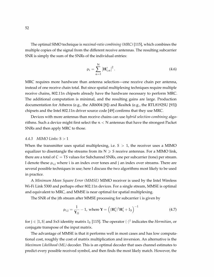
52

The optimal SIMO technique is maximal-ratio combining (MRC) [115], which combines themultiple copies of the signal from the different receive antennas. The resulting subcarrierSNR is simply the sum of the SNRs of the individual entries:

ρi =

N∑a=1

∣∣H ′i,a∣∣2 . (4.6)

MRC requires more hardware than antenna selection—one receive chain per antenna,instead of one receive chain total. But since spatial multiplexing techniques require multiplereceive chains, 802.11n chipsets already have the hardware necessary to perform MRC.The additional computation is minimal, and the resulting gains are large. Productiondocumentation for Atheros (e.g., the AR6004 [8]) and Realtek (e.g., the RTL8192SU [93])chipsets and the Intel 802.11n driver source code [49] confirms that they use MRC.

Devices with more antennas than receive chains can use hybrid selection-combining algo-rithms. Such a device might first select the n < N antennas that have the strongest PacketSNRs and then apply MRC to those.

4.4.3 MIMO Links: S > 1

When the transmitter uses spatial multiplexing, i.e. S > 1, the receiver uses a MIMOequalizer to disentangle the streams from its N > S receive antennas. For a MIMO link,there are a total of C = TS values for Subchannel SNRs, one per subcarrier (tone) per stream.I denote these ρi,j where i is an index over tones and j an index over streams. There areseveral possible techniques in use; here I discuss the two algorithms most likely to be usedin practice.

A Minimum Mean Square Error (MMSE) MIMO receiver is used by the Intel WirelessWi-Fi Link 5300 and perhaps other 802.11n devices. For a single stream, MMSE is optimaland equivalent to MRC, and MMSE is near optimal for spatial multiplexing.

The SNR of the jth stream after MMSE processing for subcarrier i is given by

ρi,j =1

Yjj− 1, where Y =

((H ′i)

†H ′i + IS)−1

(4.7)

for j ∈ [1,S] and SxS identity matrix IS [115]. The operator (·)† indicates the Hermitian, orconjugate transpose of the input matrix.

The advantage of MMSE is that it performs well in most cases and has low computa-tional cost, roughly the cost of matrix multiplication and inversion. An alternative is theMaximum Likelihood (ML) decoder. This is an optimal decoder that uses channel estimates topredict every possible received symbol, and then finds the most likely match. However, the

53

ML decoder has added complexity that scales with the size of the constellation, i.e., is expo-nential in the number of bits per symbol k. In the initial 802.11n chipsets, ML decoding wasconsidered too complex to be practical, but this outlook has recently changed. Today, Intel’sIWL6300 (successor to the IWL5300 I use) uses ML decoding for the smaller constellationsfor which it is practical. Atheros uses a “simplified maximum likelihood detector” [7, 8] forall modulations that approximates ML performance but has lower complexity.

The task of estimating the per-stream SNR of the output from a maximum likelihooddecoder is non-trivial. Existing estimation techniques, such as the approximation by Redlichet al. [94], have the same complexity as the full ML receiver, and are hence impractical forsoftware implementation (though they may be suitable for use if implemented in hardware).

Instead, I observe that maximum likelihood decoding can be approximated as a ≈3 dBgain over MMSE for typical MIMO systems [65]. Thus, the practical solution I proposefor my model is to always compute Effective SNR estimates using MMSE, and insteadadapt the decision thresholds τm to reflect the use of ML decoding. This approximation isimprecise—the gains of ML will vary depending on the particular channel—but allows themodel to flexibly handle many device implementations (even hybrid MMSE/ML such as inthe IWL6300). The error is likely to be small for most channels.

4.4.4 Summary

In this section, I explained how to determine the Subchannel SNRs given Effective CSImatrices for Wi-Fi links. The SISO matrices give the Subchannel SNRs directly, and I assumethe use of MRC when modeling SIMO processing. For MIMO links, the model will alwaysuse the MMSE formula given by Equation 4.7 to compute the Subchannel SNRs, thoughsome receivers may use ML instead. But since the difference between ML and MMSE is oftenjust a few dB, the model will assume MMSE and instead represent the gains from using MLby having lower Effective SNR thresholds. I describe how the sender and receiver mightcommunicate these thresholds later in this chapter. Before doing so, I will next describethe last component of my model needed to make application decisions over a space ofconfigurations.

4.5 Applications: Adapting CSI to Compute Effective CSI

Recall that for a given CSI measurement and a target configuration, the Effective CSI is thechannel state information that would be measured if the link operated in that configuration.The last few sections have described how to compute the model output given the EffectiveCSI; the final missing piece is to actually compute the Effective CSI (H ′). To compute H ′,I adapt the CSI (H) to reflect the difference between the configuration in which H wasmeasured and the target configuration. Here, I explain how to perform this step for an

54

illustrative set of configuration problems.

Antenna Selection. There areM columns andN rows in the CSI matrix H; each correspondsto one transmit or receive antenna. To compute the Effective CSI that would be used under aparticular antenna selection, we simply pick the subset of rows and columns that correspondto the desired antennas. Note that this includes both transmit antenna selection (e.g., whenS < M, pick the best S of the M transmit antennas to send with) and receive antennaselection (e.g., whenN > S, turn off the least useful of the excess antennas in order to reducepower consumption).

Channel Width Selection. In 802.11n, a full 40 MHz CSI measurement comprises 114 matri-ces Hi. To implement channel width selection, we use only the Hi covered by the potentialchannel. For the lower 20 MHz channel, we would use the matrices corresponding toi ∈ [1, 56]; for the upper 20 MHz channel we would use the matrices for i ∈ [59, 114]. (Sub-carriers 57 and 58 are not part of either 20 MHz channel because the 40 MHz channel doesnot need the same guard band.) This method can also predict performance using 5 MHz or10 MHz channels as in 802.11j or SampleWidth [21], and could support a potential futureversion of 802.11 that allows the devices to use non-contiguous tones as in SWIFT [90].

Transmit Power Control. If the transmitter changes the amount of power it radiates, thischange will be reflected as simple scaling of the received CSI. Recall that each entry in Hrepresents an amplitude (also a phase), which has a quadratic relationship with transmitpower. Thus when the transmitter reduces the transmit power uniformly across subcarriers,say by 3 dB (a factor of 2), we multiply each matrix by the square root of the power change,in this example by

√2. To model the effects of asymmetric power control across subchannels,

e.g., water filling across streams or subcarriers, we can apply scaling differently to differentparts of the channel matrix.

MCS (Rate) Selection. For any of the above transmitter and receiver configurations, mymodel can predict whether a particular MCS will reliably deliver packets. The CSI matrixmay need to be slightly modified depending on the MCS, however. For instance, when usingmultiple streams the total amount of power is generally kept constant, so the Effective CSImust include a division of the transmit power across antennas. Similarly, some chipsets (e.g.,IWL5300 and the Atheros-based Ubiquiti SR71-A [116]) are unable to send at full powerwhen using the highest modulations, because the peak-to-average power ratio (PAPR) ishigher than the transmit amplifier(s) can support. For these chipsets, the Effective CSI mustbe scaled to compensate for the reduced transmit power when predicting the performanceof the relevant modulations.

Spatial Mapping. Spatial mapping algorithms determine how the different transmit streams

55

are mapped to transmit antennas. These are implemented by the MxS matrices Vi, suchthat the Effective SNR is

H ′i = HiVi. (4.8)

I discuss the four types of spatial mapping techniques from the simplest to the most general.

• In direct mapping, the transmitter maps each spatial stream directly to one of S antennas;excess antennas go unused. After choosing the appropriate rows of H as described aboveunder transmit antenna selection, the matrix V is the identity matrix IS. We can combinetransmit antenna selection and direct mapping using aMxSmatrix V consisting of zerosexcept for the S entries in different rows and columns that indicate which streams aremapped to which antennas. For S = 2 and M = 3, a direct mapping matrix using thefirst and third antennas would be

V =

1 00 00 1

. (Combined 3x2 TX Antenna Selection and Direct Mapping)

• In indirect mapping, the S streams are mapped to S antennas but in such a way as to bespread over multiple antennas. For instance, the IWL5300 uses the following indirectmapping for 3 streams and 20 MHz channels:

V =

e−i2π/16 e−2iπ/(80/33) e−2iπ/(80/3)

e−i2π/(80/23) e−2iπ/(48/13) e−2iπ/(240/13)

e−i2π/(80/13) e−2iπ/(240/37) e−2iπ/(48/13)

. (IWL5300 3x3)

Atheros uses Walsh (also called Hadamard) spreading. The 2x2 mapping is:

V =

(1 11 −1

). (Atheros 2x2)

• When using spatial expansion, S spatial streams are mapped toM > S transmit antennas.Here, V is the product of an expansion matrix and one of the direct or indirect mappingmatrices above. I show the case of S = 2 and M = 3 using a sample expansion matrixfrom the 802.11n standard:

V = V ′√

23

1 00 11 0

, (3x2 Spatial Expansion)

56

where V ′ is a direct or indirect mapping matrix. The√

2/3 factor above represents theeven spreading of the power from 2 streams across 3 antennas.

• Finally, beamforming is a general technique for mapping streams to antennas. Beamform-ing can be thought of as a synthesis of indirect mapping, spatial expansion (if applicable)and transmit power control. The distinctive feature of beamforming compared with theabove is that it is channel-aware; in other words, the beamforming matrix is chosen toimprove performance based on the known current channel H. This means that beamform-ing can use different mapping matrices Vi for each subcarrier, unlike the prior techniqueswhich are applied uniformly across tones. There are a large variety of techniques thatuse beamforming to improve the channel, but all can be represented in matrix form.

Higher-level Tasks. To solve configuration problems that require the composition of multi-ple measurements, such as channel selection, path selection, or access point selection, wecan repeat the steps above. For instance, two devices that wish to find the operating channelon which their link is fastest need only frequency-hop in unison and take CSI measurementsfor each frequency. They can then use the model to predict the achievable bitrate of eachmeasured operating channel and select the fastest.

4.6 Protocol Details

In this section I make concrete the actual protocols and algorithms by which my EffectiveSNR model can be used. Decisions about which configuration to choose can be made byeither end of the link, and each has its advantages. I begin by presenting an algorithmicoverview of my model and the set of information needed to compute it. I then discusstransmit-side and receiver-side procedures for calculating the Effective SNR, includingwhat information needs to be communicated between endpoints (and when that exchangehappens) for these approaches to work.

4.6.1 Protocol Overview

I present the skeleton of a procedure to use my Effective SNR model as Algorithm 4.2.We can define a configuration problem as a set of configurations under consideration (C)and some metric (M) that enables us to choose between configurations.

Consider the example problem of rate selection over a three-antenna 802.11n link. For thisapplication, we define C to be the 24 modulation and coding scheme (MCS) combinationsthat span all SIMO, MIMO2, and MIMO3 rates. (This assumes only 20 MHz channels andthat the receiver is fixed to use all three antennas.) For metric M, we use the threshold-basedmetric given in Algorithm 4.1. Then Algorithm 4.2 will use my Effective SNR procedure ona measured 3x3 channel matrix H and return the configuration predicted to be the fastest.

57

Algorithm 4.2 EFFECTIVE SNR ALGORITHM SKELETON

1: Define an application by a set of configurations C and a metric M

2: Measure the CSI H, covering the subchannels used in all configurations3: for configuration ci ∈ C do4: Use the Effective SNR model and H to determine ρeff,c // Note that ci specifies a choice

of rate, sender configuration (including channel), and receiver configuration.5: Set metricmi to M(ci, ρeff,ci)6: end for7: return the configuration ci with the best metricmi

Note that Algorithm 4.2 uses the brute-force approach of checking all configurations tofind the best one. For extremely large search spaces, it may be necessary to prune the searchspace if computation time dominates the rate at which the channel changes. However notethat this inflection point comes for much larger spaces than the probe-based approach, sinceEffective SNR can predict the performance of many configurations using a single packetpreamble, while probe-based algorithms must send one or more full-length packets to test aconfiguration.

In order to actually run this procedure, three pieces of information are necessary inpractice:

1. Up-to-date CSI measurements including all relevant subchannels.

2. The receiver’s MCS-specific Effective SNR thresholds.

3. Knowledge of how to compute the Effective CSI H ′ from the CSI H.

A challenge is that this information is spread across the transmitter and receiver. In particular,CSI measurements are naturally measured at the receiver in the course of receiving 802.11npackets, and I envision that the receiver’s Effective SNR thresholds will be programmed inat the factory since they are fixed and independent of channel conditions. At the same time,computing the Effective CSI requires knowledge of transmitter behavior, including spatialmapping matrices as well as any implementation-specific oddities. The latter can be quitebroadly defined, such as Intel’s reduction of transmit power by up to 5 dB for the highest64-QAM single-stream encodings to compensate for amplifier non-linearities. Finally, whichendpoint applies the result of the computation depends on the application in mind. Oftenthe adjustment will be at the transmitter side, such as choice of rate, but some applications,such as receive antenna selection, are applied at the receiver.

In the next few subsections, I first discuss how CSI is obtained, as this is the mainrun-time measurement needed to run this algorithm. I then describe the transmitter- and

58

receiver-side ways to implement Algorithm 4.2 and the tradeoffs of the various approaches.The primary tradeoff is between the amount of data shared (because the party performingthe calculation needs up-to-date CSI) and protocol complexity.

4.6.2 CSI Collection

As with RSSI, receivers gather channel state information automatically while receiving apacket; the OFDM and MIMO equalizers described in Section 4.4 fundamentally rely onCSI to decode the received signal. This passive collection of CSI via overheard transmissionssuffices for most applications, such as rate selection. When a more comprehensive CSImeasurement is needed, the transmitter can send a sounding packet [45: §20.3.13.1] at awider bandwidth or using more streams to probe the extra dimensions. For the special caseof measuring additional spatial streams, 802.11n includes a mechanism to send a modifiedpacket with extension spatial streams [45: §20.3.9.4.6] such that the receiver can measure thefull channel during the preamble but that does not change the rate or number of streamsused for the data portion.

4.6.3 Transmitter-side Computation

The transmitter seems to be a natural place to perform these computations, as most configu-ration points are determined by transmitter configurations. To do so, it needs an up-to-dateCSI measurement as well as the receiver’s MCS thresholds. The latter is easy: Since thethresholds are fixed for a particular model of NIC, they can be shared by the receiver once,e.g., during association.

The transmitter can obtain CSI via feedback or estimate it implicitly from the reversepath. When the receiver feeds CSI back to the transmitter, this process adds latency andreduces airtime efficiency. 802.11n includes mechanisms to limit these effects via rapidfeedback protocols [45: §9.19.2] and compressed CSI feedback formats [45: §20.3.12.2.5].Additionally, my measurements taken in conjunction with experimenters at Intel show thatin slow-fading channels, such as static nodes with indoor mobility, CSI estimates are validfor a few hundred milliseconds [85] and this may require less frequent feedback.

Alternatively, the transmitter can attempt to estimate the CSI implicitly when receivingpackets, such as ACKs, sent by the receiver. This is the standard approach taken in PacketSNR-based schemes such as CHARM [55] proposed for single-antenna 802.11a systems.For systems with multiple antennas, like 802.11n, this approach mandates that the receiverinform the transmitter of its spatial mapping matrices and use all its antennas to sendthese packets. Another approach is for the receiver to send ACKs using fewer streams,but alternate which antenna set it uses so that the transmitter can gradually build up thefull CSI; this process is called CSI Sampling and Fusion [25]. The use of implicit feedbackalso requires devices to use the 802.11n calibration process to compensate for hardware

59

differences in the measured transmit and receive chains and those that will be used whenthe two devices swap roles. Some receivers, such as the Intel IWL5100, have more receiveantennas than transmit chains and cannot send on all antennas. For these devices, implicitfeedback would simply not work.

Finally, the implicit feedback approach induces all the problems of receiver-side com-putation (see below) with few of the benefits, and I do not find it to be practical. Insteadchoosing to make decisions at the transmit side of the link, I recommend that the transmitterobtain CSI feedback explicitly when making an Effective SNR decision.

4.6.4 Receiver-side Computation

The other approach is for the receiver to perform the computations and make the applicationdecisions, feeding them back to the transmitter when necessary. This obviates sendingCSI and speeds up the protocols, but instead requires that the receiver understand thetransmitter’s behavior and capabilities.

Today, the transmitter shares some of these details, such as number of transmit antennasand whether it supports optional 802.11n features, with the receiver during association.But the standard does not include a method by which a transmitter can share its spatialmapping matrices, and it is not immediately clear that this would sufficiently capture allimplementation artifacts such as those described above.

The other drawback to this approach is that it complicates receiver algorithms. Forinstance, if the transmitter is an access point and the client a cell phone, the former deviceis likely to have much more sophisticated silicon. We have seen this today as many 802.11manufacturers have targeted systems with asymmetric capabilities such that the accesspoint shoulders all the computation load, reducing the complexity and hence cost of theclient which need only support basic functionality. The receiver-side approach requires thatthe receiver shoulder the computational load of running the model and making decisions;in contrast for the transmitter-side approach it must only support CSI feedback.

Still, I believe that the receiver-side approach is fundamentally the best. This approachhas the primary advantage of putting the computation near the data, so that rather thanfeeding back the full CSI measurement to the transmitter, the receiver need only send theapplication decision over the air. This is similar to the approach taken by RBAR [43], andsupport for this has been added to 802.11 with the new 802.11n Link Adaptation Controlfield [45: §7.1.3.5a] that can embed feedback in packet headers, including ACKs, to directlyrequest a particular MCS, select transmit antennas, or request a particular beamforming (orother spatial mapping) matrix.

To make the receiver-side algorithm work best, I suggest a simple new contract be addedto 802.11n as a standard requirement. Since today transmitters may use fundamentally

60

different spatial mapping matrices for different numbers of streams, it is hard to computethe Effective CSI for a different number of streams. Indeed, the Intel IWL5300 uses spatialmapping matrices such that the 2-stream CSI bears no obvious relation to the 3-streamCSI without knowledge of the possible mappings, and uses different matrices for 20 MHzand 40 MHz channels. In my experiments using the IWL5300, I assumed that the receiverknows the spatial mapping matrices a priori, but sharing the full extent of these mappingsis hard to fit into a clean protocol. As a cleaner solution, I propose that transmitter spatialmapping matrices be restricted such that when a receiver subsets a large (e.g., MIMO3)CSI measurement to simulate a smaller (e.g., MIMO2) configuration, the result indeedcorresponds to the channel that would be measured if the transmitter used that mode. Ithink this new contract would best resolve the situation without greatly compromisingtransmitter performance or flexibility.

4.6.5 Summary

In this section, I discussed some practical details of implementing my Effective SNR-baseddecision procedure. When comparing the transmitter-side and receiver-side options forimplementing this functionality, I concluded that receiver-side computation likely representsthe best tradeoff, because it has the benefit of low overhead without compromising onflexibility, accuracy, or agility.

In certain situations, such as when selecting beamforming matrices, the decision may bebest made at the transmitter, which better understands the limitations of its own hardware.And for multiple links to coordinate, CSI measurements may need to be shared in a localneighborhood. One example of a system that does this lightweight local sharing in order toachieve better spatial reuse is IAC [31].

4.7 Comparison to Other Techniques

I conclude this chapter by comparing my Effective SNR to other techniques that use physicallayer or other low-level information to predict the performance of a wireless link. I comparealgorithms along two axes: (1) their applicability to many configuration problems, and (2)their efficiency in terms of overheads and responsiveness.

4.7.1 Accuracy

Table 4.4 summarizes the comparison between Effective SNR and other recent algorithmsthat aim to predict the performance of a wireless link. The results show that Effective SNRcan handle a much broader problem space because it looks at the raw channel details,while other algorithms primarily apply only to single-stream links with fixed antennas andtransmit power.

61

Algorithm 802.11a/b/g802.11n Antenna

TX PowerChannel Real Wi-Fi

(MIMO) Selection Width Devices

Packet SNR ? XSoftRate [120] X

AccuRate [103] X X XEEC [22] X X

Effective SNR X X X X X X

Table 4.4: A comparison of Effective SNR to other recent algorithms that purport to pre-dict the performance of a wireless link. Effective SNR can predict packet delivery in thelargest space because it looks at the underlying subchannel response, whereas the othertechniques mostly apply to single-stream links with fixed antennas and transmit power.

Algorithm MeasurementCommunication

ComputeResponse

Overhead Time

Probe-based Multiple packet loss rate None Low HighPacket SNR Preamble Low Low High

SoftRate [120] A few full symbols Low Low LowAccuRate [103] Preamble Low Very High High

EEC [22] Full packet Low High Medium

Effective SNR PreambleLow (RX)

Medium LowMedium (TX)

Table 4.5: Comparing overheads and response times of Effective SNR and other algo-rithms. In addition to being more flexible and accurate than the other algorithms (Ta-ble 4.4), Effective SNR has low measurement and communication overheads, little com-putational cost, and low response time. This matches the best aspects of the other algo-rithms.

62

As I presented in the previous section, Packet SNR based on RSSI is available in today’sdevices, but is does not accurately predict performance for 802.11a/g due to its inabilityto capture frequency-selective fading; the use of MIMO in 802.11n only exacerbates thisdeficiency.

SoftRate [120] and EEC [22] both use information from the error correction hardware toaccurately measure the Effective BER of the current configuration. They have been shown towork well for rate selection using adjacent 802.11a/b/g rates, but they cannot predict theperformance of other configurations such as using different numbers of antennas.

AccuRate [103] uses the measured receive error vectors as input to a full channel simu-lator; like my model this procedure can estimate the Effective BER of all modulations inthe current configuration. However, these computations are computationally expensiveand do not hold across antenna modes. One case where it may work is changing channelwidth, by only using the error vectors for the desired subcarriers. AccuRate may also beable to support transmit power control: I believe this can be approximated by scaling theerror vectors, if the hardware distortion does not change across transmit powers. However,neither of these tasks were explored by the authors.

In contrast, Effective SNR applies in more settings than the other techniques because itscomputations are aware of the low-level physical-layer effects of the RF channel, includingfrequency- and spatially-selective fading. My model is broadly compatible with 802.11nand requires no hardware changes.

4.7.2 Overheads and Response Time

Table 4.5 summarizes my qualitative comparison of these algorithms in terms of theirpractical overheads and the achievable response times.

Packet SNR-based algorithms, AccuRate, and Effective SNR all require only a packetpreamble to record their measurements. SoftRate, which uses the output of the error cor-rection blocks to estimate Effective BER, requires a packet that contains at least a fewMIMO-OFDM symbols that fully utilize the available subchannels. EEC requires slightlymore bits to accurately estimate the BER (around a full packet), and the standard probe-based approaches today require multiple full-length packet probes to estimate the loss rateof a particular configuration.

None of the schemes have much additional communication overhead beyond the exist-ing 802.11 protocol, feeding back only configuration decisions or concise metrics such asSNR or BER estimates. When using Effective SNR to make decisions that require transmit-side computation (which other algorithms cannot handle at all) Effective SNR must feedCSI back to the transmitter, though the feedback can be compressed and may only need tobe sent periodically.

63

In terms of computation, Packet SNR and SoftRate require very little, either directlyfeeding back the hardware’s estimate to the other side of the link or performing a simplelocal threshold test. Today’s probe-based algorithms require a small amount of computationto update loss rate estimates. Among the rest, AccuRate has such a large overhead as tomake it impractical, because it requires a full wireless channel simulator of a full-lengthpacket in order to compute its output. EEC’s custom codes require a medium amount (about250µs) of computation [22], which is longer than a packet sent at 58.5 Mbps but still quickerthan a full 4 ms packet batch. In contrast, I will show in the next chapter that the EffectiveSNR computations for rate selection among 24 MCS combinations can be computed inunder 4µs, around the time for a single MIMO-OFDM symbol. Both EEC and EffectiveSNR computations would be faster if implemented in hardware instead of in software on adesktop computer, but Effective SNR can already be calculated fast enough for real-timeadaptation in fast-changing channels.

Finally, I compare the algorithms on the basis of their responsiveness. The algorithmsthat are more accurate—SoftRate, AccuRate, EEC, and Effective SNR—can respond quicklyto changing conditions. However, this applies only to those configurations they can solve(see Table 4.4), and the response time of AccuRate and EEC are limited by their computationtime. In contrast, because probe-based algorithms must search a large space and PacketSNR-based algorithms require online training of SNR thresholds, they cannot respond in anagile way in mobile environments.

4.8 Summary

This section has presented my Effective SNR model and how to use it. The key idea is touse CSI measurements made by the receiver from a single packet preamble to efficientlyinfer how well other configurations would work. When used with my Effective SNR model,the CSI can easily and efficiently handle a wide range of transmitter, receiver, and rateconfigurations. My model provides a flexible API to support many different configurationtasks and includes considerations for real receivers with practical implementations operatingover real wireless channels.

I concluded with a comparison of my Effective SNR-based model to other techniqueswith similar goals. Effective SNR can handle a much larger problem space than comparablealgorithms, because my model is able to capture the underlying RF details of the MIMO-OFDM channel, rather than high-level observations of the channel, packet delivery, or errorrates. In terms of overheads and response time, Effective SNR comes close to matching thebest of the other algorithms, with the upside of having wider applicability to new Wi-Fitechnologies.

Of course, I have not yet shown that my Effective SNR model is accurate. In order to

64

understand whether this is the case, I built a prototype implementation of my model usinga commercial Intel wireless chipset. In the next chapter I describe this implementation. I usethis implementation in the rest of this thesis to demonstrate that my Effective SNR modelworks well and supports a wide space of applications.

65

Chapter 5

EXPERIMENTAL PLATFORM

In this chapter, I describe my experimental 802.11n platform, which comprises a proto-type implementation of a CSI measurement tool based on commodity Intel Wi-Fi chipsetsand experimental 802.11n wireless testbeds in two indoor office environments. This ex-perimental setup is the foundation for the experimental results in the remainder of mythesis.

5.1 Experimental 802.11n Wireless Testbeds

I conducted experiments in two 802.11n stationary wireless testbeds. (In addition to thesetwo stationary testbeds, I use three laptops for mobile experiments; I describe their configu-ration in the next section.)

The first testbed, pictured in Figure 5.1(a), contained 10 nodes spread over one floor ofIntel Labs Seattle covering 8,100 square feet. In the second testbed, I deployed 24 nodesacross 3 floors in UW CSE (Figure 5.1(b)), where each floor measures approximately 20,000square feet in size. Both locations are indoor office buildings, the former mostly a wide openarea with cubicles and a few conference rooms, the latter consisting primarily of 5-personoffices.

Each node runs the experimental platform described below in Section 5.3. In bothtestbeds, I placed the nodes to ensure a large number of links between them, a varietyof distances between nodes, and diverse scattering characteristics. Devices are located ondesktops, under tables, on a cart in the server room, and even mounted on the ceiling.The UW CSE testbed also includes a more dense concentration of nodes in one area of thebuilding (pictured in the upper right corner of Figure 5.1(b)), making it a highly diversetestbed and increasing the challenge of configuration.

5.2 Node Configuration

Each node is a stationary desktop (Figure 5.2) or portable laptop (Figure 5.3) equipped withan Intel 802.11n wireless network interface card (NIC) that supports three antennas. As theantenna geometry of a multi-antenna device is important for spatial diversity, I mount thethree antennas per node on custom stands. Each antenna achieves 5 dBi gain for the 2.4 GHzband, and 3 dBi for the 5 GHz band.

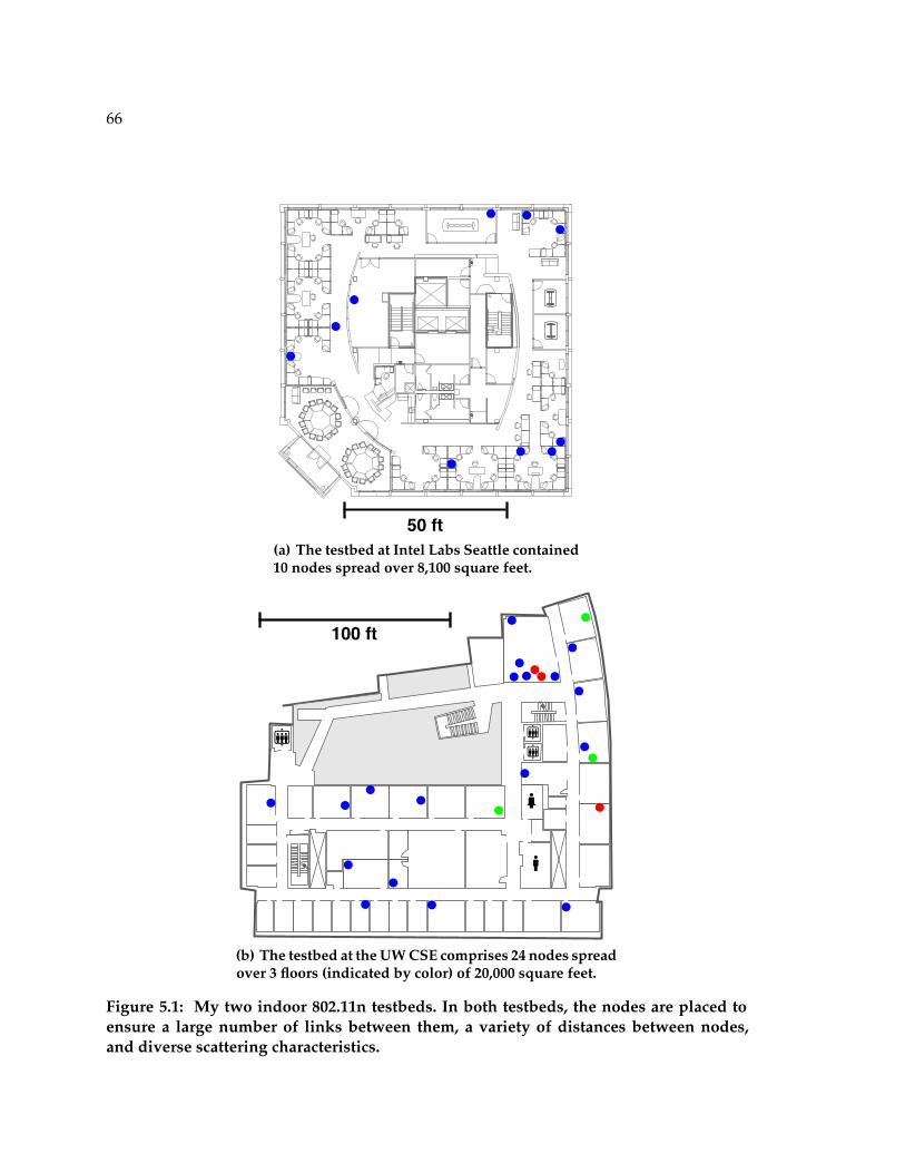
66

50 ft(a) The testbed at Intel Labs Seattle contained10 nodes spread over 8,100 square feet.

100 ft

(b) The testbed at the UW CSE comprises 24 nodes spreadover 3 floors (indicated by color) of 20,000 square feet.

Figure 5.1: My two indoor 802.11n testbeds. In both testbeds, the nodes are placed toensure a large number of links between them, a variety of distances between nodes,and diverse scattering characteristics.

67

Figure 5.2: The antenna stand I use to achieve consistent spatial geometry for desktopmachines. It supports circular and linear arrays of two or three antennas with the correctλ/2 separation at either 2.4 GHz or 5 GHz.

Figure 5.3: One of the three laptops, pictured here, includes a custom antenna mount fora 2.4 GHz linear array.

The desktop stands (Figure 5.2) allow for a circular array (using ports ABC) or a lineararray of two or three (AB2 and optionally center) antennas, with antenna separations ofhalf the wavelength for either 2.4 GHz Channel 6 (λ/2 = 6.15 cm) or 5 GHz Channel 48(λ/2 = 2.86 cm). In desktop experiments in this paper, I use the circular three-antennaconfiguration for the 2.4 GHz band. It is robust and suited to dual-band chips that need thewider 2.4 GHz antenna separation.

The three laptops use three different antenna configurations. One laptop has all threeantennas embedded internally like in a commercial laptop deployment; one laptop usesthe same antenna stand as the desktop machines to mimic their behavior in portableexperiments. The third laptop, pictured in Figure 5.3, includes a custom antenna mount fora 2.4 GHz linear array. For mobile experiments, I use the laptop with internal antennas; theother two are used as portable (but not mobile) testbed nodes to supplement the stationarytestbed.

68

Figure 5.4: The Intel Wireless Wi-Fi Link 5300. This 802.11n device has three trans-mit/receive antennas, operates on both 2.4 GHz and 5 GHz frequency bands, and sup-ports up to three spatial streams for a maximum bitrate of 450 Mbps.

5.3 Node Software: 802.11n CSI Tool and Research Platform

In conjunction with Intel Labs Seattle, I built an experimental 802.11n platform that uses theIntel Wi-Fi Wireless Link 5300 (IWL5300) 802.11a/b/g/n network cards (Figure 5.4). These802.11n MIMO chipsets have three antennas and support many new features of 802.11n. Imodified the closed-source firmware and open-source iwlwifi driver for Linux to add anumber of experimental features and, crucially, to measure the 802.11n CSI.

802.11n CSI Measurement. The channel sounding mechanism added in 802.11n definesa management frame used to report the CSI from the receiver of a frame back to thetransmitter. This mechanism is intended for calibration or to inform transmit beamforming,and I co-opt it for my experiments. In standard operation, the CSI is reported only when thesounding procedure is initiated by the transmitter, though the receiver measures CSI forevery frame in order to receive the packet. In my tool, I configure the NIC with a debugmode to compute this feedback packet for every received frame, rather than just duringsounding. For correctly received packets, the firmware will send the measured CSI up tothe driver on the receiving node, which forwards it to a userspace application that can logor process the CSI.

In my tool, CSI feedback is not returned to the transmitter by default. Instead, theuserspace application that processes CSI can optionally generate feedback (potentiallyincluding Effective SNR or rate selection information rather than simply the measured CSI)and return it to the transmitter.

The IWL5300 provides CSI in a format that reports the channel matrices for 30 subcarriergroups, which is about one group for every 2 subcarriers at 20 MHz or every 4 subcarriersat 40 MHz. Each channel matrix entry is a complex number, with signed 8-bit resolution

69

each for the real and imaginary parts. It specifies the gain and phase of the spatial pathbetween a single transmit-receive antenna pair. Intel’s implementation of the 802.11n CSIdoes not include per-subcarrier noise measurements, so I assume the noise floor is uniformacross all subcarriers to compute SNRs. This is consistent with white noise observed onother OFDM platforms [89].

RSSI Measurement. For each received packet the NIC reports the traditional metrics ofRSSI per receive antenna, noise floor and the setting on the automatic gain controlled (AGC)amplifier. These combine to define the per-receive-chain Packet SNR (ρpacket):

ρpacket = RSSI (dBm) − Noise (dBm) − AGC (dB) (5.1)

The IWL5300 calculates the quantities RSSI and Noise as the respective sums of averagesignal strength and average error vector magnitude in each OFDM subcarrier [49]. This isexactly the traditional definition of SNR applied to OFDM.

Note that with multiple receive antennas, there is a different RSSI and hence a differentPacket SNR for each antenna. As described below in Section 5.4.1, I compute the PacketSNR for the link by summing the Packet SNR of the antennas.

Transmit Power Control. I modified the driver and firmware to enable transmit powervariation. With these changes, I can vary the transmit power level from −10 dBm (100µW)to +16 dBm (40 mW) in steps of 0.5 dB. For all modulations, the IWL5300 divides powerequally across transmit antennas. Additionally, the IWL5300 reduces the transmit powerslightly when using the highest single-stream rates to avoid distortions caused by passing64-QAM symbols with high peak-to-average power ratio through the transmit amplifier.

Rapid Rate Variation. In normal operation, the IWL5300 decouples queuing packets fortransmission from selecting rates for these packets, since queues must be kept large totake advantage of 802.11n block transmissions. This makes it difficult to control the rate atwhich individual packets are transmitted. I modified the firmware and driver to supportthe transmission of individual packets at predetermined rates, and added driver-level codeto rapidly iterate through a user-configurable set of available rates.

Userspace Connector. I used the Linux kernel connector framework to implement alow-latency socket-based communication channel between the kernel driver and userspaceutilities. This enables userspace utilities to log CSI and other output from the driver, and tosend messages that adapt behavior of either end of the link online, e.g., by changing thecurrently selected rate or antennas or adjusting the transmit power level.

Publicly Released Tool. I have publicly released the experimental platform and CSI collec-tion tool in the form of open source drivers, userspace utilities, MATLAB data processing

70

code, and binary firmware image [37]. At the time of writing, I am aware many users ofthe tool: 20 universities in 7 countries, multiple research and product groups within Intel,one industrial research lab, and one startup. The users of my tool have published at least 7papers [13, 25, 32, 85, 100, 102, 124].

5.4 Computing 802.11n SNR and Effective SNR using IWL5300 Measurements

In the rest of this thesis, I use measurements from my experimental platform to evaluatehow well Effective SNR (and other algorithms) work for real 802.11n wireless channels. Inmost experiments, I computed the packet reception rate (PRR), Packet SNR, and EffectiveSNRs for all the measured configurations. The packet reception rate is easy to compute bysimply counting the number of correctly received frames compared to the number sent.The rest of this section describes practical considerations when computing Packet SNR andEffective SNR values.

5.4.1 Processing Multiple RSSIs to Compute Packet SNR

When receiving a transmission with multiple antennas, there is one RSSI value per antenna;how should these measurements be combined into a single SNR value for the link? Asdescribed above, I first convert the per-antenna RSSI and noise measurements to SNRs(Equation 5.1) and then sum the SNRs. This is a straightforward choice for a single spatialstream as it corresponds to receiver processing using maximal-ratio combining (Equa-tion 4.6). It is also reasonable for 2- and 3-stream MIMO because the symbols carried ondifferent spatial streams are interleaved coded bits [45].

5.4.2 Processing CSIs to Compute Effective SNRs

The 802.11n standard mandates that CSI measurements, which are stored as matrices of 8-bitcomplex numbers indicating gain and phase of each subchannel, include a per-subcarrierSNR reference that enables the grounding of each per-subcarrier channel matrix, such thateach entry in the CSI can be treated as a magnitude relative to the noise floor. It is underthis model that the equations I presented in Chapter 4 hold.

In attempting to use the measured CSI from the Intel NICs, I discovered a practicalissue that needed to be taken into account: Quantization error. This issue is a fundamentalproblem that applies to all uses of CSI in the 802.11n standard. Consider a very strong link,say with a signal-to-noise ratio of 50 dB. Most actual receiver processing occurs after thissignal has been digitized by the analog-to-digital converter (ADC) at each receive chain; thisconversion from analog to digital cannot be perfect, and thus induces quantization errorin the digital signal. For instance, a 12-bit ADC can represent signal levels from −2048 to+2047, with an error up to ±0.5. Note that the analog gain control (AGC) hardware on thechip aims to amplify the received analog signal to fully utilize the ADC range.

71

An error of ±0.5 in a measured magnitude of up to 2048 corresponds to a quantizationerror of about −72 dB. Roughly, each bit that the ADC outputs gives a 6 dB reduction inquantization error, because it halves the relative error in magnitude, dividing the power ofthat error by a factor of 4, i.e., 6 dB.

How does quantization error compare to the noise floor? The answer is that it dependson the strength of the link and the ADC output. For the link above with an SNR of 50 dB,a 12-bit ADC corresponds to a quantization error 72 dB below the signal strength, hence22 dB below the noise floor. This is essentially no additional error at all. In contrast, a 6-bitADC would cause quantization error 36 dB below the signal strength, which is 25× largerthan noise power for this very strong link! So, in some cases it can be important to takequantization error into account when using CSI measurements.

My results later in the thesis show that accounting for quantization error indeed im-proves the accuracy of Effective SNR predictions considerably. I achieved the best resultswhen I assumed that the IWL5300 NIC in my testbed used a 6-bit ADC.

5.4.3 Computing Effective SNR

Taking into account quantization error, I used the processed and corrected CSI1 to computeEffective SNR values for links in my testbed according to the model described in Chapter 4.I parameterized the model with known properties of the Intel IWL5300 devices: They useminimum mean square error (MMSE) MIMO equalizers, and have known, fixed spatialmapping matrices that I detail in the tool source code [36: matlab/sm_matrices.m].These are the CSI measurements I use in the remainder of this thesis.

5.5 Summary

This chapter described my 802.11n experimental platform and CSI measurement tool, anddetailed a number of practical considerations that are important when computing PacketSNR and Effective SNR values on real hardware. In the rest of this thesis, I use thesemeasurements to evaluate whether my Effective SNR model is accurate and how well itworks relative to other algorithms for a variety of configuration problems.

1 A second issue is an implementation artifact of the way that the Intel chip reports channel state information.The SNR reference is missing from each subcarrier’s CSI matrix, and instead all matrices are normalized to anunknown reference. I determined via trial-and-error that this reference value is the total RSSI and developeda procedure to normalize it [36: matlab/get_scaled_csi.m].

72

73

Chapter 6

EVALUATING EFFECTIVE SNR FOR MIMO-OFDM CHANNELS

In this chapter, I experimentally evaluate how well my Effective SNR model predictspacket delivery for 802.11n wireless links.

To do so, I use my CSI measurement tool to gather a wide range of channel and perfor-mance information across 200 wireless links in both testbeds. This captures a wide varietyof fading environments, from line-of-sight links in the same room to links between nodes indifferent rooms with RF barriers and reflectors spread around and between them. I use thisdata to evaluate the accuracy of predictions made using Packet SNR and Effective SNR.

The primary study in this chapter determines how accurately Effective SNR predictswhether packets will be delivered using different modulation and coding schemes. The goalis that for every modulation and coding scheme (MCS), a clear Effective SNR thresholdseparates those links that do not deliver packets at that rate from those that do, and thusthat my model is accurate for practical links. Using these thresholds, I determine how wellEffective SNR can identify the MCS with the highest throughput. I also compare how wellPacket SNR works when used in the same way.

I next consider how well my model enables predictions about the effects of transmitpower control on rate. This joint optimization problem highlights my model’s flexibility. Iconclude this chapter by evaluating the resilience of my Effective SNR system to interference,so that it can still be used to make predictions in contested wireless environments.

Combined, these three studies lay the foundation for showing that Effective SNR isaccurate, flexible, and practical.

6.1 Experimental Data

I measured packet delivery over a 20 MHz channel on my two 802.11n testbeds, using linkswith four different antenna configurations:

1. The SISO configuration uses a single antenna at each node. This configuration corre-sponds to 802.11a.

2. The SIMO configuration uses a single transmit antenna but three receive antennas.This is an 802.11a/g/n configuration that uses spatial diversity techniques.

3. The MIMO2 configuration uses two spatial streams and three receive antennas. This

74

employs both 802.11n techniques of spatial multiplexing and spatial diversity.

4. The MIMO3 configuration uses three antennas at each node to send and receive threespatial streams. This configuration uses spatial multiplexing but does not benefit fromspatial diversity.

For each of these configurations, I measured the packet delivery for each link usingeach MCS, at each transmit power level between −10 dBm and +16 dBm in steps of 2 dB.I sent 1,500-byte packets as constant bit-rate UDP traffic generated by iperf at 2 Mbpsfor 5 seconds, about 860 packets total. The receiver also recorded the CSI and per-antennaRSSIs and noise floors to measure the RF channel for each correctly received packet. Inthese experiments, I turned off 802.11’s link layer retransmissions in order to observe theunderlying packet delivery rate. The experiments were conducted at night on unused 802.11channels in order to minimize the effects of environmental movement and RF interferenceon these results.

The above tested across 200 links, 26 dB of transmit power, four antenna configurationsranging from SISO to MIMO3, and 8 MCS values per configuration. This covers all of thekey variables needed to implement and evaluate my Effective SNR model.

6.2 Packet Delivery with Effective SNR

The first study in this chapter aims to understand whether Effective SNR is a good metric,i.e., whether it is an accurate predictor of packet delivery. In this section, I evaluate themodel in three ways. The first is via the transition window, i.e., the SNR regime in whichpacket delivery for all links goes from near-zero to near-perfect. We saw in Chapter 3 thatthis transition occurs rapidly for a wired link (Figure 3.7), but occurs over a wide range forwireless links (Figure 3.8) when using the Packet SNR. A narrow transition window thatmatches measurements of Packet SNR over a wire would be one indicator that EffectiveSNR works well.

The second evaluation metric is rate confusion, i.e., how many rates might be best at aparticular SNR value. The example wired link showed clear separation between rates, suchthat at every SNR value there is a clear best rate. Conversely, because the transition regionsof different wireless links overlap, links with the same SNR might support very differentrates.

Finally, I determine the SNR thresholds for each MCS and use them to predict the rateconfiguration with the highest throughput for each link. The accuracy of this prediction is acore measurement of how well an SNR metric can inform decisions.

For all of these analyses, I evaluate the predictions made by my Effective SNR modelindependently and as compared to Packet SNR.

75

0

20

40

60

80

100

0 5 10 15 20 25 30 35

Pa

cke

t R

ece

ptio

n R

ate

Packet SNR (dB)

MCS 0

MCS 1

MCS 2

MCS 3

MCS 4

MCS 5

MCS 6

MCS 7

Figure 6.1: A scatterplot of packet reception rate versus Packet SNR for wireless linksin the testbed. There are wide transition regions and significant overlap between rates.

6.2.1 Transition Windows

I begin with a visual comparison of the transition regions for real wireless links, and thenpresent a quantitative evaluation of the difference between Packet SNR and Effective SNR intransition window width. I focus on SISO links, for which the most testbed links transitionfrom being lossy to reliable. I examine the remaining configurations in the next section.

Visual Comparison

Recall Figure 3.8 from Chapter 3, which shows a scatterplot of packet reception rate (PRR)as a function of Packet SNR for three sample single-antenna modulations in the testbedsdescribed in Chapter 5. This graph demonstrated that for real wireless links, the width ofthe transition region is 10 dB or more, so that there is a large range of power levels for whichPacket SNR does not predict performance.

In Figure 6.1, I present a version of that plot that now includes data points for all eightmodulation and coding scheme (MCS) combinations. In this graph, we can see that there isa correlation between Packet SNR and rate, but there is also a significant overlap betweenrates. For most MCS values, the transition region is at least five and often ten dB wide. For alarge SNR range, many links will be lossy using one rate, while other links will work well atthe next higher, or even the second higher, rate. This illustrates why Packet SNR computedfrom RSSI does not provide a good indicator of performance across testbed links in practice.

Contrast this with Figure 6.2, which shows the exact same set of data points but usingEffective SNR instead of Packet SNR along the x-axis. This picture now shows a muchclearer separation between rates. Especially for lower MCS values, only a few outlier linksoverlap with the next higher rate. Note also that, as shown in Chapter 4, the Effective SNR

76

0

20

40

60

80

100

0 5 10 15 20 25 30 35

Pa

cke

t R

ece

ptio

n R

ate

Effective SNR (dB)

MCS 0

MCS 1

MCS 2

MCS 3

MCS 4

MCS 5

MCS 6

MCS 7

Figure 6.2: A scatterplot of PRR versus Effective SNR for the same wireless links. Rel-ative to Packet SNR, there are narrower transition regions and cleaner separation be-tween rates. The overlap that is present is generally between links that use the samemodulation but different coding schemes (see Table 2.2).

is several decibels lower than the Packet SNR because it measures the amount of power thatis actually harnessed by the link, rather than the total power.

In both graphs the separation is generally larger between rates that use different modula-tions, e.g., between MCS 2, which uses QPSK, and MCS 3, which uses 16-QAM. In contrast,rates that only differ in coding rate overlap to a more substantial degree. This effect is worstfor the highest rates (MCS 5–MCS 7), which use 64-QAM modulation. I believe this artifactis fundamental, as it matches the results from the wired link (Figure 3.7); I attribute it to thefact that these three MCS use coding rates 2/3, 3/4, and 5/6 that are much closer togetherthan the 1/2-coded and 3/4-coded combinations used for the QPSK and 16-QAM rates.

Quantitative Evaluation

The visual comparison presented above shows qualitatively that Effective SNR provides amore compact transition region and clearer separation between rates, but note that scatter-plots can be misleading because they obscure density and distributions—each plot abovehas 16,188 points. To understand the data quantitatively, I analyzed the SISO measurementsto find the transition window for each of the measured links.

Formally, I define the transition window of a particular rate to be the set of SNR valuesbetween which packet delivery rises from 10% (lossy) to 90% (reliable) for any link. Table 6.1gives the width of the transition window (denoted ∆ρ) for SISO rates using the Packet SNRand Effective SNR metrics. I show the 25th–75th percentile range of points in the transitionwindow as a measure of the typical link, and the 5th–95th range as a measure of most

77

MCS Rate (Mbps)∆ρpacket (dB) ∆ρeff (dB)

5%–95% 25%–75% 5%–95% 25%–75%

0 6.5 3.08 1.29 2.05 0.811 13.0 3.45 1.44 2.38 0.892 19.5 6.27 3.12 2.30 0.853 26.0 3.93 1.98 3.02 0.944 39.0 7.05 3.49 2.19 0.935 52.0 7.16 3.20 2.29 1.066 58.5 7.25 3.37 2.92 1.417 65.0 7.24 2.81 2.92 1.35

Average 5.68 2.59 2.51 1.03

Table 6.1: A table of the widths of SISO transition windows.

links. A good result here is a narrow 1 dB–2 dB window like that measured over a wire(Figure 3.7).

The table shows that the transition widths are consistently tighter with my model thanwith Packet SNR. Most links transition within a window of around 2 dB for most rates. Thewidth of the SNR-based transition windows is typically two to three times looser, especiallyfor the denser modulation schemes like 64-QAM and higher code rates. At higher rates, it iseasy for a sub-ideal channel to degrade packet reception. However, while the transitions forthe last four rates are high with Packet SNR, they remain tight with Effective SNR.

Limits on Accuracy

In Table 6.1, the transition regions for Effective SNR range from 1 dB to about 3 dB, de-pending on the MCS value. In fact, these results for Effective SNR are about the best thatcan be obtained because they are close to textbook transitions for flat-fading channels andthose measured over a wire (Figure 3.7). A small improvement is surely possible, but this isprobably limited by the precision of my measurement data. The IWL5300 gives RSSI, AGCand noise values in dB to the nearest integer, and outputs at most 8-bit CSI over a 48 dBrange for only 30 out of 56 subcarriers. With this combination of factors, a CSI quantizationerror of at least 1 dB is likely.

Summary

This section showed that my Effective SNR model provides a channel metric that cannarrow transition windows and shows a separation between rates. The larger significanceof narrow transition windows is that, by reducing them enough that they do not overlap,I can unambiguously predict the highest rate that will work for nearly all links nearly all

78

of the time. In contrast, Packet SNR transition windows overlap such that for a given SNRthere may be many different best rates for different links in the testbed. I explore this next.

6.2.2 Rate Confusion

To understand whether my Effective SNR model accurately predicts packet delivery, Ianalyze the fastest working rate (PRR> 90%) for each link and all NIC settings. If weconsider the set of all links that have the same SNR value (binned in groups of 1 dB), thebest link is the link with the fastest working rate, and the worst link is the slowest. Ideally,SNR would perfectly indicate rate and all links with the same SNR would have the samebest rate, but in practice there is a gap; this gap is the rate confusion.

In Figure 6.3, I show the rate confusion by plotting the rate versus SNR for the bestand worst links, broken down by configuration. Recall that to measure PRR I sent over 800packets for each link in transmitter configuration. To assign a single Packet SNR or EffectiveSNR value to the trace, I choose the median measurement over all successfully receivedpackets. The SISO experiment (Figure 6.3(a)) shows links for both testbeds combined. Theremaining graphs (Figure 6.3(b)–6.3(d)) show rates for SIMO, MIMO2 and MIMO3 configu-rations for the Intel testbed only; it is denser than UW and supports MIMO experimentsover the IWL5300’s transmit power range. Note that the SIMO figure does not include datafor the lowest 6.5 Mbps rate because, with the high degree of spatial diversity, very fewlinks experience loss at that rate within the transmit power range of the IWL5300.

For the SISO (Figure 6.3(a)) and MIMO3 (Figure 6.3(d)) cases, the figures show that usingPacket SNR results in a large spread between the best and worst lines. Except for extremelylow and high SNRs, nearly all SNRs have at least two—and up to five different—rates assuitable choices for the best rate. That is, Packet SNR often poorly indicates rate.

In sharp contrast, the two Effective SNR lines overlap almost all the time, and mostlyappear to be a single line. This is almost an ideal result. Effective SNR is a clear indicator ofbest rate. When there is slight separation, the spread is only between rates that use the samemodulation but different amounts of coding, just as I described in the last section. Thesecombinations are also close together in our wired experiments.

Interestingly, these results show that Packet SNR predictions are much better for theSIMO and MIMO2 cases, though still not as accurate as Effective SNR, particularly forthe highest rates. The reason is spatial diversity: Spare receive antennas gather the receivedsignal and combine it to make the channel more frequency-flat [35], thus bringing thePacket SNR closer to the Effective SNR. This effect is well-known, though typically notobservable using real 802.11 NICs which, except my prototype implementation, do notexport CSI. This result suggests that Packet SNR is a reasonable predictor for an 802.11configuration with significant diversity, using RSSI measured in that configuration. Still,

79

0

6.5

13

19.5

26

39

52

58.5

65

0 10 20 30 40 50

SIS

O B

itra

te

Effective SNR (dB)

Best Link

Worst Link 0

6.5

13

19.5

26

39

52

58.5

65

0 10 20 30 40 50

SIS

O B

itra

te

Packet SNR (dB)

Best Link

Worst Link

(a) SISO configurations

0

6.5

13

19.5

26

39

52

58.5

65

0 10 20 30 40 50

SIM

O B

itra

te

Effective SNR (dB)

Best Link

Worst Link 0

6.5

13

19.5

26

39

52

58.5

65

0 10 20 30 40 50

SIM

O B

itra

te

Packet SNR (dB)

Best Link

Worst Link

(b) SIMO configurations

0

13

26

39

52

78

104

117

130

0 10 20 30 40 50

MIM

O2 B

itra

te

Effective SNR (dB)

Best Link

Worst Link 0

13

26

39

52

78

104

117

130

0 10 20 30 40 50

MIM

O2 B

itra

te

Packet SNR (dB)

Best Link

Worst Link

(c) MIMO2 configurations

0

19.5

39

58.5

78

117

156

175.5

195

0 10 20 30 40 50

MIM

O3 B

itra

te (

Mbps)

Effective SNR (dB)

Best Link

Worst Link 0

19.5

39

58.5

78

117

156

175.5

195

0 10 20 30 40 50

MIM

O3 B

itra

te (

Mbps)

Packet SNR (dB)

Best Link

Worst Link

(d) MIMO3 configurations

Figure 6.3: Rate confusion with Packet SNR and Effective SNR. Excepting very low andhigh SNRs, one Packet SNR value maps to multiple best rates for different links, thoughit works better in configurations that use spatial diversity (SIMO and MIMO2). For thesame data, Effective SNR provides a clear indicator of the best rate for nearly all links.

80

Packet SNR does not transfer well across the antenna modes, because diversity gains andinter-stream interference change unpredictably. This makes Packet SNR less useful as amethod of selecting rates, as we will see in the next section.

6.2.3 Selecting Rates

In Section 6.2.1, I showed that transition regions for Effective SNR are generally tighter thanfor Packet SNR. In Section 6.2.2 I showed that Effective SNR as a channel measure has lessrate confusion relative to Packet SNR. These results indicate that a threshold-based EffectiveSNR algorithm should be better able to distinguish whether a particular MCS combinationworks for most links. In this section, I show how to choose SNR thresholds and analyzewhether these thresholds lead to good choices for real wireless links in my testbeds.

Choosing SNR Thresholds

The first question is how we should choose the SNR thresholds needed in Equation 4.3 todecide whether a link will reliably deliver packets in a particular configuration. A low SNRthreshold will lead to aggressive rate selection, with many false positives as transmitters sendat a rate faster than their links support, and widespread packet loss. A high SNR thresholdwill cause many false negatives, in which transmitters select rates conservatively and sendmore slowly than necessary. In this thesis, I use a simple heuristic: Choose thresholds tobalance the prevalence of false positives and false negatives.

To find the threshold for a particular MCS value, I use the following procedure. Definegood links to be those links with PRR >90%. The CDF of the SNR values for these links thenindicates the false negative rate; choosing the 25th percentile SNR as the threshold meansthat the 25% of links that have lower SNR values will be falsely classified as not working.Similarly, we can define bad links to be those with PRR <80%. Then the CDF of the SNRvalues for these links shows the inverse of the false negative rate; the 25th percentile SNRwould falsely classify the 75% of links with larger SNR values as good links. To balancefalse negatives and false positives, we can plot the CDF of SNR values for good links andthe complementary CDF of SNR values for bad links on the same graph. The x-coordinateof the intersection point of the two lines is the SNR threshold that balances false positiveand false negative error rates, and the y-coordinate of that point gives the balanced error rate.An ideal result is a balanced error rate of 0%, so that the SNR threshold perfectly classifiesall links as working or not.

Figure 6.4 shows the error rate versus Packet SNR for the SIMO, MIMO2, and MIMO3configurations, and Figure 6.5 shows the same data using Effective SNR. Unlike in Sec-tion 6.2.2, the Packet SNR or Effective SNR value used to make these graphs is taken from asingle MIMO3 packet. To compute Effective SNR for SIMO and MIMO2 configurations, Icompute the SIMO and MIMO2 Effective CSI as described in Chapter 4. For Packet SNR, I

81

use the measured Packet SNR for all antenna configurations, as the transmitter keeps thetotal radiated power constant across antenna modes.

The results show that both SNR metrics have a balanced error rate under 14% for allconfigurations. Effective SNR has a lower error rate for all but the lower MIMO2 rates,often much lower. We also see that both schemes perform worst for the highest MCScombinations in each antenna mode that use 64-QAM with close coding rates. This matchesthe expectations from earlier sections.

I plot the CDF of the balanced error rate for each scheme in Figure 6.6. The balancederror rate curve is generally 1%–2% less for Effective SNR than for Packet SNR. I also plotthe relative balanced error rate of Effective SNR compared to Packet SNR in Figure 6.7. Thisgraph shows that the Effective SNR balanced error rate is as low as 40% of that achievedwith Packet SNR, and less than 10% worse for the single rate where that is the case. Thus, itseems likely that my threshold-based Effective SNR model will be a better predictor of linkperformance than using thresholds with Packet SNR. I investigate this next.

Using Thresholds to Select Rates

Having computed the Packet SNR and Effective SNR thresholds for each MCS value, I nowevaluate how well the chosen rates work in my testbed.

I used the thresholds computed above to choose rates for 2163 links in my wirelesstestbed. These are the links that support at least 6.5 Mbps, so they can deliver packets, butare not so strong that the fastest rate works perfectly, so that rate selection is meaningful.I follow the procedure in Algorithm 4.2: Given a single Packet SNR or Effective SNRmeasurement from each trace, predict how well each configuration works and then choosethe fastest one. I compare to the ground truth optimal rate for each link, computed by usingthe packet reception rates described earlier to compute the actual performance of each rate.

Figure 6.8 shows the results when selecting rates using Packet SNR or Effective SNR.The graph contains one line for each algorithm. A point (x,y) on a line means that thecorresponding algorithm achieves at least an x fraction of optimal performance for a yfraction of links. An ideal result would be a vertical line x = 1, showing that all links achieveoptimal performance.

In this graph, we see that Effective SNR dramatically outperforms Packet SNR. Themedian link in our testbed achieves 83% of optimal performance using rates selected withEffective SNR, while using Packet SNR for rate selection results in a median performance of13%. With Packet SNR, nearly half the links choose rates that deliver no packets at all, whileEffective SNR is so excessively aggressive for less than 10%. Though there is still a sizablegap from optimal, this experiment highlights that Effective SNR performs much better thanthe Packet SNR, even when using only a single channel measurement and no adaptation of

82

0

2

4

6

8

10

12

14

-5 0 5 10 15

Err

or

rate

(%

)

Packet SNR

False Pos.

False Neg.

0

2

4

6

8

10

12

14

5 10 15 20

Packet SNR

0

2

4

6

8

10

12

14

5 10 15 20

Packet SNR

0

2

4

6

8

10

12

14

5 10 15 20

Packet SNR

0

2

4

6

8

10

12

14

5 10 15 20

Err

or

rate

(%

)

Packet SNR

0

2

4

6

8

10

12

14

10 15 20 25

Packet SNR

0

2

4

6

8

10

12

14

15 20 25 30

Packet SNR

0

2

4

6

8

10

12

14

20 25 30 35

Packet SNR

0

2

4

6

8

10

12

14

0 5 10 15 20

Err

or

rate

(%

)

Packet SNR

0

2

4

6

8

10

12

14

5 10 15 20

Packet SNR

0

2

4

6

8

10

12

14

5 10 15 20

Packet SNR

0

2

4

6

8

10

12

14

5 10 15 20

Packet SNR

0

2

4

6

8

10

12

14

10 15 20 25

Err

or

rate

(%

)

Packet SNR

0

2

4

6

8

10

12

14

15 20 25 30

Packet SNR

0

2

4

6

8

10

12

14

20 25 30 35

Packet SNR

0

2

4

6

8

10

12

14

25 30 35 40

Packet SNR

0

2

4

6

8

10

12

14

10 15 20 25

Err

or

rate

(%

)

Packet SNR

0

2

4

6

8

10

12

14

10 15 20 25

Packet SNR

0

2

4

6

8

10

12

14

15 20 25 30

Packet SNR

0

2

4

6

8

10

12

14

15 20 25 30

Packet SNR

0

2

4

6

8

10

12

14

20 25 30 35

Err

or

rate

(%

)

Packet SNR

0

2

4

6

8

10

12

14

25 30 35 40

Packet SNR

0

2

4

6

8

10

12

14

25 30 35 40

Packet SNR

0

2

4

6

8

10

12

14

30 35 40 45

Packet SNR

Figure 6.4: False negative and false positive error rates as a function of Packet SNRthreshold. The figure shows results for wireless links that use one- (top), two- (middle),and three-stream (bottom) rates (MCS 0–MCS 23).

83

0

2

4

6

8

10

12

14

0 5 10 15 20

Err

or

rate

(%

)

Effective SNR

False Pos.

False Neg.

0

2

4

6

8

10

12

14

0 5 10 15

Effective SNR

0

2

4

6

8

10

12

14

0 5 10 15

Effective SNR

0

2

4

6

8

10

12

14

5 10 15 20

Effective SNR

0

2

4

6

8

10

12

14

5 10 15 20

Err

or

rate

(%

)

Effective SNR

0

2

4

6

8

10

12

14

10 15 20 25

Effective SNR

0

2

4

6

8

10

12

14

10 15 20 25

Effective SNR

0

2

4

6

8

10

12

14

15 20 25 30

Effective SNR

0

2

4

6

8

10

12

14

-5 0 5 10

Err

or

rate

(%

)

Effective SNR

0

2

4

6

8

10

12

14

-5 0 5 10

Effective SNR

0

2

4

6

8

10

12

14

0 5 10 15

Effective SNR

0

2

4

6

8

10

12

14

0 5 10 15

Effective SNR

0

2

4

6

8

10

12

14

5 10 15 20

Err

or

rate

(%

)

Effective SNR

0

2

4

6

8

10

12

14

10 15 20 25

Effective SNR

0

2

4

6

8

10

12

14

10 15 20 25

Effective SNR

0

2

4

6

8

10

12

14

15 20 25 30

Effective SNR

0

2

4

6

8

10

12

14

-5 0 5 10

Err

or

rate

(%

)

Effective SNR

0

2

4

6

8

10

12

14

-5 0 5 10

Effective SNR

0

2

4

6

8

10

12

14

0 5 10 15

Effective SNR

0

2

4

6

8

10

12

14

0 5 10 15

Effective SNR

0

2

4

6

8

10

12

14

5 10 15 20

Err

or

rate

(%

)

Effective SNR

0

2

4

6

8

10

12

14

10 15 20 25

Effective SNR

0

2

4

6

8

10

12

14

10 15 20 25

Effective SNR

0

2

4

6

8

10

12

14

10 15 20 25

Effective SNR

Figure 6.5: False negative and false positive error rates as a function of Effective SNRthreshold. The figure shows results for wireless links that use one- (top), two- (middle),and three-stream (bottom) rates (MCS 0–MCS 23).

84

0

0.2

0.4

0.6

0.8

1

0 2 4 6 8 10 12 14

CD

F o

ver

MC

S c

om

bin

ations

Balanced error rate (%)

Effective SNR

Packet SNR

Figure 6.6: Balanced error rates for Ef-fective SNR and Packet SNR in wirelesstestbed links.

0

0.2

0.4

0.6

0.8

1

0.4 0.5 0.6 0.7 0.8 0.9 1 1.1

CD

F o

ve

r M

CS

co

mb

ina

tio

ns

Relative balanced error rate

Figure 6.7: The balanced error rate for Ef-fective SNR relative to Packet SNR inwireless testbed links.

0

0.2

0.4

0.6

0.8

1

0 0.2 0.4 0.6 0.8 1

CC

DF

over

2163 lin

ks

Fraction of optimal performance

Effective SNR

Packet SNR

Figure 6.8: The performance of selecting rates based on Effective SNR and Packet SNRthresholds for 2163 wireless testbed links.

85

rates. (I explore rate adaptation in detail the next chapter.)

To understand how much the particular choice of threshold affects both algorithm, Iexperimented with raising or lowering the SNR thresholds uniformly across the differentMCS choices. Raising the Effective SNR thresholds by 1 dB results in more conservativechoices of rate and improved average performance: Fewer links achieve maximum perfor-mance, but the worst links that were over-selecting improve to a larger fraction of optimal.However, raising or lowering the Packet SNR had little effect on the curves in Figure 6.8,which suggests that the balanced error rate technique achieves locally-optimal thresholds.

Why does Effective SNR choose rates so much better than Packet SNR? The key reasonis that Effective SNR is able to compute a different Effective CSI for each modulationand number of spatial streams based on the particular subchannels used. This means thatEffective SNR can make decisions about each configuration independently, and hence canrecognize when fading will make a strong link work poorly in one antenna mode but notanother. In contrast, there is no way using RSSI measurements alone to predict Packet SNRin different configurations. Packet SNR must make a decision independent of fading, whichoften results in overly-aggressive choices.

This dramatic difference in performance highlights the key strength of Effective SNR:Its ability to predict performance in a wide space. Though this example only includedselecting rates keeping all other metrics fixed, subsequent studies will consider additionaldimensions of the wireless configuration space.

6.2.4 Summary

In this section, I analyzed whether Effective SNR accurately predicts packet delivery. Ifound that viewing wireless links through the lens of Effective SNR can lead to visualseparation between rates and narrow transition regions within rates. The second part ofthis study showed that Effective SNR is a clear indicator of rate, usually narrowing downthe possible set of best rates to one or two MCS within an antenna configuration. The thirdanalysis showed that Effective SNR results in generally good choices for rate (median 83%of optimal), while Packet SNR often chose rates that simply did not work (median 10% ofoptimal).

In the rest of this chapter I demonstrate that Effective SNR has a few other usefulproperties that other channel metrics do not, namely that it can be used to solve jointoptimization problems such as between transmit power and rate, and that the estimates itprovides are robust to interference.

86

0

1

2

3

4

5

6

7

8

9

10

0 5 10 15 20 25 30

Eff

ective

SN

R (

dB

)

Packet SNR (dB)

Figure 6.9: Effective SNR (for QPSK) versus Packet SNR for flat (left) to faded (right)links.

6.3 Transmit Power Control

The data above showed that my Effective SNR model can predict delivery for measurementstaken over a range of transmit powers, among other choices of rate and spatial streams. Inow show apply this model to the joint interaction of transmit power and rate, and I showthat CSI measured at one transmit power level is useful to predict delivery at a differentpower level. This is valuable for power control applications, e.g., pruning excess power toreduce co-channel interference. Earlier work has shown that Packet SNR based on RSSIdoes not do this well [77, 91, 110].

6.3.1 Transmit Power Control in Faded Channels

First, I analyze the effect of changing transmit power in faded channels. To do this, I simplyscale the CSI measured at maximum transmit power for a link and compute the resultingEffective SNR over a range of power levels.

I found that changing transmit power has a different effect (in terms of delivery andhighest rate) on different testbed links even if they start at exactly the same rate and SNRvalue. Figure 6.9 plots the Effective SNR versus Packet SNR relationship for six exampleSISO links from my 802.11n testbeds, chosen to represent a range of frequency-selectivefading profiles similar to those in Figure 3.9. The links range from nearly flat to deeplyfaded. Correspondingly, they have different slopes.

On the left, Packet SNR matches Effective SNR for the nearly flat link. Since all subcarri-ers have the same strength, this link can be modeled as a single carrier with a single BER,and hence scaling transmit power has a linear effect on the Effective SNR. However, for theright-most, deeply faded links, the Packet SNR decreases from 25 dB to 15 dB (10× transmit

87

0

0.2

0.4

0.6

0.8

1

0 2 4 6 8 10 12 14 16 18 20

CD

F o

ver

links

Power saving (dB)

Eff SNR - 0.5dBMeasured (Optimal)

Eff SNRPkt SNR

(a) Predicted and measured power saving

0

0.2

0.4

0.6

0.8

1

50 60 70 80 90 100

CD

F o

ver

links

Packet reception rates (percentage)

Eff SNR - 0.5dBMeasured (Optimal)

Eff SNRPkt SNR

(b) Measured PRR corresponding to reduced TXpower levels

Figure 6.10: Power saving and performance impact of pruning excess transmit power.Pruning with Effective SNR is tight (within 0.5 dB) and does not degrade performance.Pruning with packet SNR degrades performance more without much extra savings.

power reduction) between the dashed lines, while the Effective SNR only drops by 4 dB(2.5×). This occurs because reducing the power has different effects on error rate at differentSNR levels (see Figure 2.3)—so additional power has less impact on strong subcarriers thanon weak subcarriers. This difference in how well devices harness power across links makestransmit power control non-trivial and explains why it has been hard for prior algorithmsto use measurements at one SNR value to predict how well links will work at a differentpower level.

6.3.2 Making Predictions with Effective SNR

I test the ability of Effective SNR to make predictions across power levels by consideringthe goal of trimming excess transmit power. Excess transmit power is power that can beremoved without causing the highest rate for the link to drop.

These experiments start with 88 SISO links from the Intel Labs testbed configured toradiate 10 mW of transmit power. I then take a single CSI sample per link. Consideringtransmit power reductions in increments of 2 dB, I use the threshold-based Effective SNRand Packet SNR algorithms to predict the best supported rate for each reduced power level,and choose the lowest power level with the same best rate. The measurements describedearlier include the ground truth packet reception rate for each power level and thus theycan be used to check the accuracy of the predictions.

Figure 6.10 shows the power savings and performance degradation of four differentthreshold schemes. A good result here is power savings without a loss of performance;the absolute amount of power savings is not meaningful as it depends on the testbed andthe link. The Measured (Optimal) line shows the best that can be done. Measured PRRsat all power levels are used to guide power control decisions. Therefore, the final delivery

88

probabilities are hardly decreased (all links have PRR >90%). Most links save a little power,and some save a lot.

The graphs show that using Effective SNR to predict how much power to trim has asimilarly good tradeoff. Impact on rate remains limited, yet power is saved, more than10 dB for around 10% of the links. The gap between the Measured and the Eff SNR lines isbecause Eff SNR thresholds might be slightly conservative for some links.

To show that this trimming is tight, I considered the effect of using more aggressive—i.e.slightly lower (0.5 dB)—Effective SNR thresholds. This operation results in little additionalpower savings, but degrades performance for many more links.

Finally, I compared this algorithm to a scheme that uses Packet SNR to save power. Theresults show Packet SNR the savings are roughly similar, but more links have degradedperformance and several stop working altogether.

6.4 Interference

I conclude this chapter by investigating how my Effective SNR-based model can cope withinterference. This challenge is one of the largest potential weaknesses of this technique,because Effective SNR is based on measurements taken only during the packet preamble.There are three important components of dealing with interference, which I approach inturn.

6.4.1 CSI During Interference

The first question is: If a weak interferer occasionally transmits while a packet is beingreceived, does this weak transmission cause wild swings in the predicted link quality?

I studied the variation of CSI measurements during transient interference. I chose twonodes at UW that do not detect each other with carrier sense, and alternately designated oneas the transmitter and the other as the interferer. The nodes were configured to send largepackets designed to collide, while all other receiving nodes monitored the CSI to simulate atotal of 20 links. The experiment also varied the transmit power of the node designated asthe interferer from low to high to induce a large range of interfering channels, over which Ievaluate the impact of interference on CSI measurements and my Effective SNR model.

For all but one of 20 links, the rate predicted by my model for the majority of correctpackets was the same with and without interference; the remaining link was off by a singlerate. In other words, the interference does not corrupt the CSI measurements, because theMIMO-OFDM training procedure can fairly accurately estimate CSI. Note that OFDM doesnot turn interference into inflated RSSI, unlike the spread spectrum modulations used in802.11b. From these measurements, we can conclude that the mere presence of interferencedoes not completely invalidate Effective SNR values, and thus transient interference will

89

not necessarily cause wild swings in the recommend transmit configuration.

6.4.2 Recognizing Collisions

A second task is to recognize collisions when they occur, in order to distinguish betweentoo-aggressive rate selection and interference loss. The solutions to these problems are verydifferent. To work around persistent collisions from hidden terminals, a transmitter increasesits MAC backoff counter and/or initiates the RTS/CTS procedure which is normally dis-abled for protocol efficiency. In contrast, when rates are over-selected the transmitter shouldreduce its rate but ideally need not add additional protocol delay. Accurately distinguishingbetween these two effects is known to improve performance in practice [50, 120, 123].

To recognize collisions, I propose to leverage a new MAC feature of the 802.11n packetaggregation mechanism. Block ACKs selectively acknowledge frames in a batch of packetstransmitted as one continuous burst. Each packet in the burst has a separate checksum,and thus the Block ACK serves as block-based feedback of packet correctness just likethe block-based checksums analyzed in PPR [50]. We can therefore use the error patternsin the Block ACK to recognize collisions: When the rate is over-selected, errors shouldbe randomly distributed throughout the batch, and bursty when a collision clobbers acontinuous part of the batch. The ability to recognize interference and hence decoupleinterference avoidance and rate selection has been shown to improve performance in manysystems (e.g., SoftRate [120]).

6.4.3 Effective SINR

The final task is to dealing with persistent interference, i.e., if the RTS/CTS procedure doesnot successfully avoid collisions. For continuous interference the Effective SNR computedfrom CSI will likely provide an aggressive estimate, and the system will need another wayto compensate. It may be possible to use an Effective Signal-to-Interference-and-Noise Ratio(Effective SINR) metric that incorporates CSI measurements from the interfering nodes topredict packet delivery taking into account the MIMO-OFDM fading properties of both thedesired signal and any interfering transmissions. I leave the investigation of this techniqueto future work.

6.5 Summary

From the studies in this chapter, I conclude that Effective SNR consistently provides accurateestimates of packet delivery for nearly all links and all configurations without any per-linkcalibration. Viewing diverse wireless links in my testbeds through the lens of Effective SNRshowed that there is a low degree of rate confusion and narrow transition region, contraryto the same results with Packet SNR. I presented my method to choose Effective SNRthresholds, and showed that Effective SNR can select rates that work well for most testbed

90

links. The results in Section 6.3 demonstrate the flexibility of this approach by showing thatCSI measurements are valid not just across different rates, but also across transmit powerscaling. Finally, I discussed three ways in which my Effective SNR model, in conjunctionwith 802.11n protocol features, can work well in the presence of interference, though I leavedetailed investigation of this problem for future research.

In the remainder of this thesis I evaluate the ability of Effective SNR to solve a variety oftasks. In the next chapter, I deploy my model as part of a rate adaptation system that selectsthe operating rate for a wireless link in mobile channels.

91

Chapter 7

RATE SELECTION WITH EFFECTIVE SNR

In the last chapter, I showed that my Effective SNR model can accurately predict packetdelivery for 802.11n. Here I close the loop, demonstrating how my model can be applied tosolve an 802.11n configuration problem.

This chapter presents an in-depth study of the application of Effective SNR to theproblem of rate selection for 802.11. This is a fundamental, well-studied problem becauseselecting a good rate at which to encode data is crucial for a link to work perform well, andif links do not perform well then no higher-level applications can be built. Though there is awide variety of rate control algorithms, these probe- and channel-based schemes generallydo not extend well to 802.11n and/or fast mobile channels.

I first compare an Effective SNR-based rate selection algorithm against state-of-the-artschemes for single-antenna 802.11a/g systems, which generally work well for SISO links.The goal is to show that Effective SNR performs as well as or better than these existing,well-studied probe- and channel metric-based schemes on their home ground, while mymethod has the advantages of simplicity, deployability, and generality.

I then show that my Effective SNR model extends well to 802.11n (MIMO), where otherschemes do not work well. The results in this chapter will show that Effective SNR providesan accurate and response rate selection algorithm that provides good performance acrossSISO and MIMO configurations and a range of mobile channels.

In the next chapter, I will explain how to apply Effective SNR to a set of other configura-tion problems.

7.1 Experimental Methodology

I experiment with Effective SNR, an algorithm based on my model, plus SampleRate [14],the de facto rate selection algorithm in use today, and SoftRate [120], a research algorithmwith the best published results.

I implemented a version of Effective SNR that randomly probes other antenna modes tocollect CSI, and that sends Effective SNR estimates back to the transmitter. I ran it onlineagainst SampleRate in a human-scale mobility test. The results showed that the probingand feedback have little penalty: Effective SNR works better than SampleRate by a small(5%–10%) margin.

92

For a detailed comparison of Effective SNR with other algorithms, I turn to simulations.This is for two reasons: First, SoftRate runs on a software-defined radio, and cannot beimplemented on a currently available commercial 802.11n NIC. Second, I want to comparethe algorithms over varied channel conditions, from static to rapidly changing, to assesshow consistently they perform. No algorithm will beat SampleRate by a significant marginon static channels, because it will eventually adapt to the channel. In contrast, SoftRateperforms well even when the channel is changing rapidly. However, it is hard to generatecontrollable experiments in high-mobility settings. Traces let us perform these comparisonsdirectly.

In this section, I first describe the rate selection (or adaptation) algorithms studied, andthen present my trace-driven simulator that I use to perform the comparisons between thedifferent strategies.

7.1.1 Rate Selection Algorithms

SampleRate [14] is an implicit feedback scheme that uses only information about packetreception or loss to guide rate selection. It maintains delivery statistics for different ratesto compute the expected airtime to send a packet, including retries. It falls back to a lowerrate when the airtime of the chosen rate exceeds (due to losses) the airtime of a lower rate.Standard implementations send a packet to probe 1 or 2 higher rates every 10 packets, todetermine whether to switch to a higher rate.

The main weakness of SampleRate is its slow reaction to change. If the wireless channelquickly degenerates, SampleRate will incur multiple losses while it falls back throughintermediate rates.1 When the channel recovers, SampleRate’s infrequent probing con-verges to the new highest rate slowly. Algorithms such as RRAA [123] aim to improve onSampleRate’s weaknesses, but they are less widely used. The version of SampleRate I testis based on the minstrel [109] implementation in the Linux kernel. For 802.11n (MIMO)links, I use a version of SampleRate adapted for multiple streams, and based on the Linuxminstrel_ht [28] algorithm.

SoftRate [120] is an explicit feedback scheme that uses information gathered duringpacket reception at a given rate to predict how well different rates will work. The input tothese predictions is the bit error rate (BER) as estimated from side information providedby the convolutional decoder. SoftRate chooses rates based on the performance curves thatrelate the BERs for one rate (a combination of modulation and coding) to another. Each ratewill be the best choice for some BER range. SoftRate has been shown to dominate trainedSNR-based algorithms such as CHARM [55], so I do not evaluate against those approaches.

1 The original SampleRate [14] did not reduce rate for retries, but some implementations [55] and the versionused in modern kernels [109] do. This turns out to be important for good performance.

93

SoftRate is defined for SISO channels, like SampleRate, and its predictions hold only forfixed transmit power and antenna modes. It does not extend to MIMO systems; instead,separate SoftRate probes would be needed for each separate antenna configuration. Ionly use it for 802.11a/g experiments. To cover the full SISO range, I extended the MITimplementation of SoftRate to the 64-QAM modulation and added support for 2/3 and 5/6rate codes.

Effective SNR uses my model in a very simple way, based on Algorithm 4.2. Givenrecent channel state information and per-MCS Effective SNR thresholds, it computes thehighest rate configuration that is predicted to successfully deliver packets. It runs at thereceiver, measuring CSI on received packets and returning rate changes to the sender alongwith the ACK like SoftRate. Finally, to protect against poor choices near a rate boundary inour model, I fall back one rate if consecutive packets must be retried and the Effective SNRlevel has not changed. This is a fixed rule.

Like SoftRate, this algorithm obviates the search phase. There is no calibration of dy-namic thresholds. This is not rate adaptation so much as rate selection that changes onlybecause it tracks the channel’s evolution. And unlike SoftRate, the predictions of the modelhold over different antenna modes. This lets it run over 802.11n rates as easily and in thesame way that it runs over 802.11a/g rates. Thus, I report results from both 802.11a/g and802.11n runs for this algorithm.

Optimal. Finally, I take advantage of simulation to add upper bounds on achievableperformance. This lets me assess how well the algorithms perform on an absolute scale.The Optimal scheme has an oracle that knows the true highest rate that can be successfullydelivered at any given time. This is of course impractical, but the simulator can provideit. The Delayed Optimal scheme knows the optimal rate that worked on the channelfor the previous packet and uses it for the next transmission; unlike Optimal, it doesnot know the future. Since SoftRate and Effective SNR use an estimate of this previouschannel state, and SampleRate infers the recent channel state, they are unlikely to beatDelayed Optimal. The gap between Delayed Optimal and Optimal is also likely to be largebecause of inherent wireless channel variability—the Optimal algorithm gets the benefit ofinstantaneous transient improvements in the channel.

7.1.2 Trace-driven Simulator

The simulator I built uses a trace from a real mobile channel and implements all algorithmsdescribed above.

Channel Trace

I collected real channel information for the simulations. I walked around UW CSE whilecarrying a laptop configured to send back-to-back small packets to stationary testbed nodes

94

that record the CSI. The CSI measures frequency-selective fading over real, varying 20 MHzMIMO channels. This is typically not observed with more narrowband experimentation, e.g.,on the USRP. Recall that CSI is estimated during the preamble of the packet transmission,independent of the modulation and coding of the payload. Therefore, the mobile transmittercan quickly cycle through all antenna configurations (SIMO, MIMO2 and MIMO3) bysending a single short UDP packet at the lowest rate for each configuration.2 This enablesfine grained sampling of the channel, approximately every 650µs. The following resultsare derived from a trace with approximately 85,000 channel measurements taken over 55seconds, spanning varying RF channels that range from the best 3-stream rates to SISOspeeds.

The measured CSI from the trace is interpolated to 56 carriers and serves as the groundtruth for the channel in the packet simulator I describe next.

Simulator

To simulate rate selection algorithms operating over a mobile channel, I built a simulatorfrom three interacting parts: (1) An 802.11n packet simulator, which determines whetherpackets will be delivered successfully given a particular instance of the wireless channel.This simulator also computes the physical-layer feedback used by the SoftRate and EffectiveSNR algorithms. (2) Implementations of the SampleRate, SoftRate, and Effective SNR algo-rithms. (3) An 802.11n MAC simulator, which maintains the state of the 802.11n protocol,including the current time, the length of transmissions, and MAC backoff parameters. TheMAC simulator acts as a bridge between the packet simulator and the rate selection algo-rithms, taking rate choices from the rate selection algorithm and returning to it informationabout packet success or failure and the appropriate physical-layer feedback at that point intime.

802.11n Packet Simulator. I wrote a custom 802.11a/g/n packet simulator in a combinationof MATLAB and the MIT C++ GNU Radio code for SoftRate. Given the CSI describinga particular wireless channel, the simulator implements packet reception as shown inFigure 7.1. This includes demodulation for BPSK through 64-QAM, deinterleaving, andconvolutional decoding with soft inputs and soft outputs. Packets are correctly receivedwhen there are no uncorrected bit errors, or else they are lost. Thus given a measured CSItrace, the packet simulator computes which MCS combinations would successfully deliverpackets for each CSI record in the trace.

The physical-layer feedback values are computed by the packet simulator. While ap-plying error correction decoding to the received bitstream, the simulator also computes

2 Cycling through antenna modes to measure the full MIMO CSI could be avoided using the 802.11n extensionspatial streams (Section 4.6.2), but the IWL5300 does not yet support this technique.

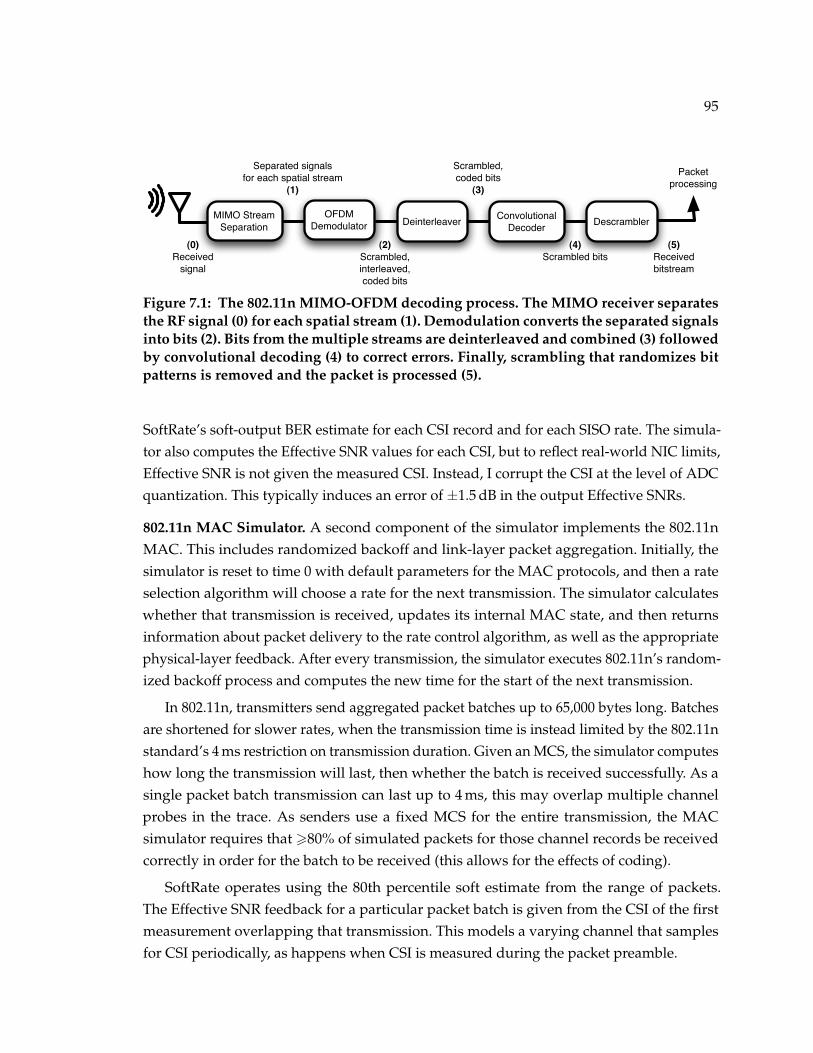
95

OFDM

Demodulator DeinterleaverConvolutional

DecoderDescrambler

(0)

Received

signal

MIMO Stream

Separation

Separated signals

for each spatial stream

(1)

Scrambled,

coded bits

(3)

(2)

Scrambled,

interleaved,

coded bits

(4)

Scrambled bits

(5)

Received

bitstream

Packet

processing

Figure 7.1: The 802.11n MIMO-OFDM decoding process. The MIMO receiver separatesthe RF signal (0) for each spatial stream (1). Demodulation converts the separated signalsinto bits (2). Bits from the multiple streams are deinterleaved and combined (3) followedby convolutional decoding (4) to correct errors. Finally, scrambling that randomizes bitpatterns is removed and the packet is processed (5).

SoftRate’s soft-output BER estimate for each CSI record and for each SISO rate. The simula-tor also computes the Effective SNR values for each CSI, but to reflect real-world NIC limits,Effective SNR is not given the measured CSI. Instead, I corrupt the CSI at the level of ADCquantization. This typically induces an error of ±1.5 dB in the output Effective SNRs.

802.11n MAC Simulator. A second component of the simulator implements the 802.11nMAC. This includes randomized backoff and link-layer packet aggregation. Initially, thesimulator is reset to time 0 with default parameters for the MAC protocols, and then a rateselection algorithm will choose a rate for the next transmission. The simulator calculateswhether that transmission is received, updates its internal MAC state, and then returnsinformation about packet delivery to the rate control algorithm, as well as the appropriatephysical-layer feedback. After every transmission, the simulator executes 802.11n’s random-ized backoff process and computes the new time for the start of the next transmission.

In 802.11n, transmitters send aggregated packet batches up to 65,000 bytes long. Batchesare shortened for slower rates, when the transmission time is instead limited by the 802.11nstandard’s 4 ms restriction on transmission duration. Given an MCS, the simulator computeshow long the transmission will last, then whether the batch is received successfully. As asingle packet batch transmission can last up to 4 ms, this may overlap multiple channelprobes in the trace. As senders use a fixed MCS for the entire transmission, the MACsimulator requires that >80% of simulated packets for those channel records be receivedcorrectly in order for the batch to be received (this allows for the effects of coding).

SoftRate operates using the 80th percentile soft estimate from the range of packets.The Effective SNR feedback for a particular packet batch is given from the CSI of the firstmeasurement overlapping that transmission. This models a varying channel that samplesfor CSI periodically, as happens when CSI is measured during the packet preamble.

96

Rate Selection Algorithms. The SampleRate, SoftRate, and Effective SNR algorithms areimplemented as described previously, and get their inputs and outputs from the packetand MAC simulator components. Each algorithm chooses a rate based on its internalstate, and the simulator returns whether the rate succeeds as well as any physical layerfeedback, namely SoftRate’s BER estimates and the Effective SNR values, measured duringthe transmission.

Metrics. The goal is to evaluate the ability of these algorithms to respond to changingchannel conditions. Thus, the primary metric is the delivered MAC layer rate per time,modeling a UDP application. Higher-layer factors, such as TCP reactions to loss, will affecthow this rate translates to throughput. These effects are ignored in the results presentedhere.

The results reported are the median of five trials where the simulator is initialized withdifferent random seeds. To vary mobility, I scale the trace at different speeds; for example, 4×mobility means that the records are assumed to arrive 4× faster than they were measured.

7.2 SISO Rate Adaptation Results

I first examine the performance of Effective SNR for selecting SISO rates. The goal of thisexperiment is to establish a reasonable baseline, showing that Effective SNR performs aswell or better than existing well-studied SISO rate adaptation algorithms, while using asimpler algorithm. If so, this will provide initial validation that the accurate packet deliverypredictions provided by my Effective SNR model are useful in practice.

7.2.1 Effective SNR vs. Optimal

I begin by comparing Effective SNR performance against the Optimal algorithm. Figure 7.2shows the rate over time for Effective SNR and Optimal over the SISO trace. The rateis averaged over a window of 200 ms to smooth the data for readability. Effective SNRperforms excellently. It is below Optimal but consistently tracks the Delayed Optimalalgorithm, a realistic upper bound. Overall, Effective SNR delivers 90% of packets, withabout 10% over-selection of rates.

Note that Packet SNR was observed to fare quite poorly in mobile channels [120]. SinceEffective SNR reflects link fading, its estimates are more accurate (Chapter 6) and are stable(2×–3× less variance).

7.2.2 Effective SNR vs. 802.11a/g algorithms

Next, I compare Effective SNR with SampleRate and SoftRate, in order to see how itperforms against current state-of-the-art SISO rate adaptation algorithms.

Figure 7.3 shows the delivered rate of each algorithm versus time. While it is hard toseparate the lines on the graph, at 1× speed, Effective SNR slightly outperforms SoftRate,

97

0

13

26

39

52

65

0 5 10 15 20 25 30 35 40

Ave

rag

e d

eliv

ere

d r

ate

(M

bp

s)

Trace index (x800)

Optimal

Delayed Optimal

Effective SNR

Figure 7.2: Effective SNR SISO performance versus Optimal in human-speed mobility.

0

13

26

39

52

65

0 5 10 15 20 25 30 35 40

Ave

rag

e d

eliv

ere

d r

ate

(M

bp

s)

Trace index (x800)

Effective SNR

SoftRate

SampleRate

SampleRate w/o fallback

Figure 7.3: Effective SNR, SoftRate, and SampleRate SISO performance in human-speed mobility.

which slightly outperforms SampleRate. These results were surprising, because the SoftRatework [120] indicated a large gap between SoftRate and SampleRate. In deeper analysis, Idiscovered that reducing the rate for retries is an important factor that gives SampleRateshort-term adaptability. Without this rate fallback (the “SampleRate without fallback” line),SampleRate loses 25%–50% of its performance in mobile channels (Figure 7.4). This variantwithout fallback is the SampleRate algorithm that was the basis for earlier comparisons.3

Figure 7.4 shows the effects of mobility on SISO channels. Each line plots the totalamount of data delivered during the trace as a function of the speed at which the trace is

3 M. Vutukuru, personal communication, and code inspection.

98

0

0.2

0.4

0.6

0.8

1

1 2 4 8 16

De

live

ry a

s f

ractio

n o

f o

ptim

al

Trace speedup

Optimal

Delayed Optimal

Effective SNR

SoftRate

SampleRate

SampleRate w/o fallback

Figure 7.4: OPT, Effective SNR, SampleRate, and SoftRate SISO performance in fastmobile channels.

played. The speeds range from 1× to 16×, corresponding to movement speeds of betweenwalking speeds ≈3 mph when using the normal simulation, to about 50 mph for the fastestplayback. The y-axis value is normalized by the Optimal algorithm’s performance to betterillustrate how the relative performance changes at different speeds.

This plot shows that all schemes fall off with increased speed; the gap between Optimaland the Delayed Optimal algorithm increases from about 20% to about 30% at the fastestspeeds. However, even in these mobile channels, Effective SNR holds up quite well andtracks the Delayed Optimal algorithm within 5%.

SoftRate performs slightly worse at the normal human speeds, but maintains a nearlyconstant performance, about 70% of Optimal, as the trace speed increases. SampleRatedegrades the fastest with increasing mobility, and the version that does not reduce rateon retries finally less than 40% of the Optimal performance, while the other algorithmsmaintain better than 60% of Optimal performance at all speeds.

Finally, I note that while the performance differences between the schemes can besignificant, other evaluations have reported larger differences. Note that they studiedthroughput based on TCP traffic, which will magnify performance gaps by reacting topacket loss. The UDP-like results I generated using my simulator capture the underlyingaccuracy of the individual schemes instead.

7.3 MIMO Rate Adaptation

Now I extend the evaluation to MIMO channels. This will show the generality of my model,which can flexibly support multiple spatial streams. I compare Effective SNR to an 802.11n-enabled version of SampleRate, to understand whether the larger search space will increase

99

0

65

130

195

0 50 100 150 200 250

Ave

rag

e d

eliv

ere

d r

ate

(M

bp

s)

Trace index (x400)

Optimal

Delayed Optimal

Effective SNR

SampleRate

Figure 7.5: Optimal, Effective SNR, and SampleRate MIMO performance in human-speed mobility.

the performance gap between the two schemes.

Figure 7.5 and Figure 7.6 show the performance of an unmodified Effective SNR algo-rithm selecting among 802.11n MIMO rates, as well as (modified) SampleRate and the twoOptimal algorithms. This graph does not include a line for SoftRate, as it is not defined formultiple streams. These figures are in the same form as for SISO, except the range of rateshas grown by a factor of 3 to support up to 195 Mbps. The MIMO trace is longer and hasmore packets-per-second, and thus includes enough data to speed up the trace by a factorof up to 256×.

Overall, the Effective SNR trends in these graphs are similar to those in the SISO graphs.At human mobility speeds, Effective SNR tracks the Delayed Optimal algorithm and deliversexcellent performance, with 75% accuracy and 10% over-selection. In faster mobile channels,Effective SNR tracks the Delayed Optimal algorithm until the speeds increase to about 128×,after which there is a slightly larger gap with for MIMO than for SISO. This arises likelybecause Effective SNR must now choose between 24 rates instead of 8. It is slightly morelikely to choose rates lower than the highest rate that would have worked.

These graphs also show that—as with SISO links—SampleRate performs well in humanspeed mobility, only slightly worse than Effective SNR. But for SampleRate, this trenddoes not hold, and as the speed of the trace gets faster the performance degrades rapidly toaround one-third of Optimal, and less than half of Effective SNR. The difference betweenSampleRate and Effective SNR highlights that Effective SNR is able to handle the largeMIMO rate space even in rapidly-changing channels, while the probe-based SampleRatealgorithm cannot.

100

0

0.2

0.4

0.6

0.8

1

1 2 4 8 16 32 64 128 256

De

live

ry a

s f

ractio

n o

f o

ptim

al

Trace speedup

Optimal

Delayed Optimal

Effective SNR

SampleRate

Figure 7.6: Optimal, Effective SNR, and SampleRate MIMO performance in faster mo-bile channels.

7.4 Enhancements: Transmit Antenna Selection

I conclude this chapter with an example that highlights the strength of my Effective SNR inthat it accommodates choices other than just rate. In particular, I amended the implementedEffective SNR algorithm to select the best transmit antenna set.

Transmit antenna selection can be useful in practice, for instance in an 802.11n AP thatselects which antennas to use to send packets to a legacy 802.11a/g client (plus uses allantennas to receive packets). With three antennas to choose from, the expected theoreticalgain in SNR is a little over 2.5 dB [30]. For a SISO link, this gain is likely enough to advanceto a higher rate.

I ran my antenna selection-enabled Effective SNR algorithm on a 3x1 MISO channel,extracted from the 3x3 MIMO trace. These measurements correspond to those that would bemeasured if the transmitter exploited the “extension spatial streams” CSI probe to measurethe 3x1 MISO channel as I described in Section 4.6.2.

Using the MISO CSI feedback, the Effective SNR algorithm chose the antenna with thehighest Effective SNR for the next transmission. This gave a gain in the total packet deliveryof 5%. For comparison, the Optimal antenna selection algorithm achieved a 10% increase byalways knowing which antenna was best.

While transmit antenna selection presents a relatively small gain for this trace, it comesat no cost and does not complicate the Effective SNR algorithm. In contrast, no other rateadaptation schemes as directly support these enhancements. They would instead requirecustomized, multi-dimensional probing algorithms and coarse adaptation of antennas toimplement antenna selection.

101

Antenna selection is one of many ways that my Effective SNR model can be appliedbeyond simple rate selection. In the next chapter, I present a study of four different networkconfiguration applications.

7.5 Summary

In this chapter, I presented a detailed evaluation of Effective SNR in the context of con-figuring the rate for 802.11a/g and 802.11n links in a mobile setting. The results for thesingle-antenna 802.11a/g systems showed that Effective SNR performs as well as or bet-ter than existing state-of-the-art algorithms for rate adaptation, with a much simpler rateselection algorithm.

A key result of this evaluation is that this good performance extends to 802.11n, whilethe probe-based SampleRate algorithm suffered in the larger search space. This validatesmy fundamental claim that probe-based algorithms will suffer in large search spaces withdynamic channels, and it motivates the need for and benefits of my Effective SNR approach.

Finally, I also showed that Effective SNR easily supports additional enhancements suchas antenna selection. In the next chapter, I will flesh out Effective SNR applications byapplying my model to a set of other configuration problems along different dimensions ofthe configuration space.

102

103

Chapter 8

FURTHER APPLICATIONS OF EFFECTIVE SNR

The detailed evaluation presented in the previous chapter showed that my EffectiveSNR model provides good performance when selecting rates for 802.11a/g and 802.11nlinks, one important application in wireless link configuration. In this chapter, I present anevaluation of the Effective SNR for four wireless configuration problems to further illustratethe broad applicability of my work.

I chose four problems that represent the key applications needed to configure a futurewireless network. The first three are selection algorithms for access points, operating chan-nels, and multi-hop paths through networks. These represent the main decisions (beyondrate) that need to be made in flexible topologies such as Wi-Fi Direct networks. The lastapplication is to classify whether a device is mobile, in order to switch between algorithmsdesigned for static vs. mobile links, or to trigger a search for a new, better operating pointwhen the device begins to move. Together these are the building blocks of an automatically-reconfiguring network that provides good performance.

8.1 Experimental Methodology

To understand how well different techniques perform at the applications studied in thischapter, I took comprehensive measurements of both packet delivery and the RF channel inthe University of Washington testbed. These data provide the ground truth performance oflinks in different configurations and also a record of the channel state during the experiments.Using this data, I perform offline simulations of the different algorithms.

8.1.1 Dataset

I measured the links between 24 static devices in my testbed at the University of Washington.The measurements in this chapter were taken 3 years after the measurements used inChapter 6 and Chapter 7, and they include a different set of devices. In addition to evaluatingthe applications in question, the results in this chapter will also tell us whether these NICsin practice experience physical degradation that invalidates their in-factory calibration.

I took measurements on all 35 channels, each 20 MHz wide, that the IWL5300 devicessupport. Of these 35 channels, 11 overlap in the 83 MHz-wide unlicensed 2.4 GHz band,and the remaining 24 non-overlapping channels are spread across three non-contiguousbands between 5.170 GHz and 5.835 GHz. In an experiment, one sender transmits packets

104

with random payloads to 23 receivers. The transmitter sends a total of 2400 packets byinterleaving 100 packets from each of the 24 MCS that correspond to 1-, 2-, or 3-stream802.11n rates. Each receiver uses 3 antennas for spatial diversity and/or spatial multiplexing.I cycled through all transmitters and all channels over the course of a few hours, and I tookdata at night to attempt to minimize the impact of interference.

The above measurements included 100 packets for each link, MCS, and channel. Fromthese data, it is straightforward to compute the ground-truth packet reception rate (PRR)for each of these configurations. In this chapter, I decouple the ability to make accuratechoices at the application-level from the rate selection algorithm needed to realize it. I thusassume an ideal rate selection algorithm that always correctly chooses the fastest MCS.This provides an Optimal baseline against which I compare Packet SNR- and EffectiveSNR-based application configuration algorithms.

8.1.2 Simulating RF Measurement-based Algorithms

While measuring the performance of the link, I sent exhaustive packet probes at all rates,and collected the RSSI and CSI for each correctly received packet. Of course, this collectedinformation would not be available to an algorithm attempting to quickly configure thenetwork. Instead, the algorithms are given only the RF measurements from the first packetreceived. I use this to compute Packet SNR (ρ) and Effective SNR (ρeff). By using only thefirst measurement, I emulate the performance that a configuration algorithm would obtainin practice, where it would use only a single probe.

In the next three sections, I evaluate how well my Effective SNR model can make accesspoint, channel, and path selections on this dataset. I use a different mobile dataset for thelast section, and describe it therein.

8.2 Access Point Selection

The first protocol operation a wireless client device performs is to join an existing network.This operation typically consists of scanning for a known access point (AP) by sendingbroadcast packets called probe requests on different frequencies until a recognized AP isfound. In a typical home today, there will likely be one valid probe response: The singlehome AP. However, in a dense Wi-Fi network, such as an enterprise Wireless DistributionSystem or a Wi-Fi Direct peer-to-peer network, the client needs to choose from among manyavailable responding devices that connect it to the same network. This is the access pointselection problem.

The general access point selection algorithm examines the probe responses to predict thelink performance for each access point, and then it chooses the fastest one (Algorithm 8.1).The standard approach used today is for the client to measure the Packet SNR from each

105

Algorithm 8.1 ACCESSPOINTSELECTION(AP SET A, SENDER s)

1: return arg maxa∈A GETMETRIC(a, s) // choose the AP with the best downlink metric

Algorithm 8.2 GETMETRIC-PACKETSNR(SENDER s, RECEIVER r)

1: Measure the Packet SNR ρ at r from s

2: return ρ

Algorithm 8.3 GETMETRIC-EFFECTIVESNR(SENDER s, RECEIVER r)

1: Measure the CSI at r from s // a full CSI including all TX and RX antennas2: Compute the Effective SNR estimates ρeff,m for each MCSm3: Determine whether each MCS works by comparing ρeff,m > τm4: return the bitrate B(m) for the fastest working MCSm

probe response and connect to the strongest AP (Algorithm 8.2). Here, SNR measurementsare used as a proxy for an estimate of the downlink throughput, and the AP with thehighest SNR is considered the best. (Other factors than link quality, such as interferenceand contention with other clients, can affect throughput as well; some systems can takethese factors into account, but they are not relevant here. I discuss these and other relatedissues in Chapter 9.) In this section, I evaluate whether using Effective SNR to predict thedownlink rate can improve this decision process (Algorithm 8.3).

8.2.1 Characterization of Access Points

I begin by characterizing whether access point selection matters in my testbed. How muchdoes a good or bad choice impact performance?

To generate data for this evaluation, I first filtered the data set to the 11 channels in the5 GHz band for which there is no overlapping UW Wi-Fi network. Then I considered theaccess point selection problem by considering each client and channel in turn. In particular,for node c playing the role of a client, I defined A to be the set of access points thatresponded to a probe from that client on a particular channel. By considering each channelindependently each client generates 11 data points, for a total of 11 ∗ 24 = 264 simulatedclient association attempts. To ensure that AP choice can matter, I excluded 17 clients thathad fewer than 3 responding APs on a particular channel, leaving 247 total.

Figure 8.1 and Figure 8.2 show the results, framed as the difference in throughput(relative or absolute) from the best choice AP for the worst, median, and average choices.These graphs show that for this testbed, choosing the wrong AP can hurt: The worstresponding AP offers less than half of the best AP’s throughput in 95% of cases, and in

106

0

0.2

0.4

0.6

0.8

1

0 0.1 0.2 0.3 0.4 0.5 0.6 0.7 0.8 0.9 1

CC

DF

over

247 c

lients

Performance relative to best AP

Worst AP

Median AP

Average AP

Figure 8.1: For each client, the relative difference in throughput over access points com-pared to the best choice.

0

0.2

0.4

0.6

0.8

1

0 25 50 75 100 125 150 175 200

CD

F o

ve

r 2

47

clie

nts

Performance less than best AP (Mbps)

Worst AP

Median AP

Average AP

Figure 8.2: For each client, the absolute difference in throughput over access points com-pared to the best choice.

most cases the random (average) and median APs are better but not close to optimal. Inabsolute terms, the downlink from the median AP is 50 Mbps to 100 Mbps worse than fromthe best AP in most cases. A poor choice of access point can dramatically hurt performancein practice.

8.2.2 Access Point Selection Performance

As presented above, Algorithm 8.1 shows the framework for selecting access points typicallyused today, with Packet SNR (Algorithm 8.2) usually used as the metric of comparisonbetween access points. I calculate the Effective SNR link metric as in Algorithm 8.3—asimple instantiation of the procedure described in Chapter 4.

107

0

0.2

0.4

0.6

0.8

1

0 0.2 0.4 0.6 0.8 1

CC

DF

over

247 c

lients

Performance relative to best AP

Effective SNR

Packet SNR

Average AP

Figure 8.3: CCDF of relative performance of AP selection using Packet SNR and Effec-tive SNR, compared to Optimal.

Figure 8.3 shows the performance of Packet SNR and Effective SNR-based access pointselection algorithms relative to the optimal algorithm. I plot the complementary CDF of theresults, so that each (x,y) point in the graph shows the fraction of clients y that achievedperformance at least within the fraction x of the optimal algorithm. The line for a perfectlyaccurate algorithm would be located in the upper right corner of the graph: All clientswould achieve the best possible throughput. This graph shows that both algorithms performwell, choosing a near optimal access point in almost all cases. I attribute this overall goodperformance to the fact that the potential access points are spread across a large testbed,exhibiting a wide range of SNRs. This large geographic spread means that there may beone or a few nearby access points that offer a clear best choice, and Packet SNR—which iscorrelated with distance—can correctly identify good choices.

Although both algorithms perform well, Effective SNR offers improved performance.The Effective SNR algorithm finds the best access point for 83% (204) of clients, versus 72%(177) for Packet SNR. Considering only the suboptimal choices, those made by EffectiveSNR are better: 3/4 (31/43) of incorrect choices are within 80% of optimal, versus only half(35/70) when using Packet SNR.

Next, Figure 8.4 shows the absolute performance loss of the two algorithms in choosingthe access point. Here, each (x,y) point represents the fraction of links y that choose anaccess point within xMbps of the best access point. The area over the curves represents theperformance lost by each algorithm: An accurate algorithm would be in the top left corner,losing little throughput for only a few links.

Examining this graph, we can see that these benefits translate to raw bitrate as well. Ac-

108

0

0.2

0.4

0.6

0.8

1

0 10 20 30 40 50

CD

F o

ve

r 2

47

clie

nts

Performance less than best AP (Mbps)

Effective SNR

Packet SNR

Average AP

Figure 8.4: CCDF of the throughput lost using APs selected by Packet SNR and EffectiveSNR, compared to Optimal.

0

0.2

0.4

0.6

0.8

1

0.4 0.6 0.8 1 1.2 1.4 1.6 1.8 2

CD

F o

ver

247 c

lients

Performance of AP selected via Effective SNR relative to Packet SNR

Figure 8.5: The relative throughput selecting APs by Packet SNR or by Effective SNR.

cess points selected by Effective SNR links are within 10 Mbps of optimal for 90% (223/247)of cases, but only 78% of selections meet this criterion when using Packet SNR. For PacketSNR, the 90th percentile performance loss is 42 Mbps, versus 9 Mbps with Effective SNR.These results show that the Effective SNR-based access point selection algorithm works welland makes better choices than one based on Packet SNR. Using the area over the curves asa measure of the inefficiency, this area is 2.7× larger when using Packet SNR.

That Effective SNR is statistically better than Packet SNR over the testbed does not meanit works better in all cases. I examine the head-to-head performance of selecting accesspoints via Effective SNR or Packet SNR in Figure 8.5. For each link, I plot the ratio of theperformance of the access point picked with the Effective SNR strategy to that of the access

109

point chosen by maximizing Packet SNR. If the two APs perform equally, the ratio will be 1;if the Effective SNR strategy chose a better AP the ratio will be larger. The algorithms choseAPs with equal performance for 69% (171/247) of the clients, Effective SNR makes a betterchoice in 21% (53) of cases, and Packet SNR is better for the remaining 10% (23). ThoughEffective SNR does not always lead to a better choice, it does so twice as often as PacketSNR. The graph also shows that when Packet SNR does make a better choice, Effective SNRcomes close—within 2/3 for 5 in 6 of these cases—while it often improves on the choicefrom Packet SNR by a larger margin.

Effective SNR occasionally worse. It may be surprising that Effective SNR, with its abilityto better understand subchannel effects, can ever result in a worse choice of access pointthan using the Packet SNR computed from RSSI. I present one likely explanation.

Recall that these algorithms compute channel metrics using a single RSSI or CSI measure-ment. Generally, a single CSI probe is not as accurate as multiple measurements, becauseof error in the estimates of individual subcarriers. On the other hand, a single RSSI probemeasures only the total power across carriers and is consistent across packets.

Summary. When selecting access points, both Packet SNR and Effective SNR make goodchoices; each algorithm selects the fastest access point in most cases. However, the ability ofEffective SNR to capture channel effects leads to better choices more often and generallycloser-to-optimal performance when it makes a choice incorrectly.

8.3 Channel Selection

Using the new Wi-Fi Direct standard, 802.11 devices that wish to send data directly (insteadof through the access point as in 802.11 infrastructure mode) can create a peer-to-peer link.Depending on the amount of interference in the network (e.g., from other clients of theaccess point) and the quality of the link between the two devices, they may wish to move thelink to a different operating channel in order to improve performance. This is one exampleof the channel selection problem: To quickly choose the best operating frequency for a pair ofnodes to communicate. In this section, I define the “best” channel to be the channel thatprovides the highest throughput in the absence of interferers.

The channel selection problem is similar to the access point selection problem, and has asimilar algorithmic solution (Algorithm 8.4). It can use the same GETMETRIC functions forPacket SNR (Algorithm 8.2) and Effective SNR (Algorithm 8.3). The primary difference isa reordering of the parameters: Rather than a fixed receiver with fixed channel choosingbetween multiple senders, a fixed sender and receiver must choose between multiplechannels.

110

Algorithm 8.4 CHANNELSELECTION(CHANNEL SET C, SENDER s, RECEIVER r)

1: for all c ∈ C do2: Both s and r switch to channel c3: Compute the channel metricmc using GETMETRIC(s, r)4: end for5: return arg maxc∈Cmc // choose the channel with the best metric

0

0.2

0.4

0.6

0.8

1

0 0.1 0.2 0.3 0.4 0.5 0.6 0.7 0.8 0.9 1

CC

DF

over

201 lin

ks

Performance relative to best channel

Worst channel

Median channel

Average channel

Figure 8.6: The relative difference in throughput over 802.11n channels.

8.3.1 Characterization of 802.11 Channels

To start my investigation of channel selection algorithms, I first measured how the operatingfrequency affects 802.11n links in practice.

As in Section 8.2, I filtered the data to the 11 channels in the 5 GHz band for which thereare no co-channel university APs. (Note that channel selection generally makes sense withinone frequency band. Selection across bands is trivial: Because of better antenna gain andFriis’ Law effects, a 2.4 GHz channel has typically 10 dB–15 dB stronger SNR than a 5 GHzchannel for the same nodes.) I further eliminated from consideration any pairs of devicesthat did not obtain at least 6.5 Mbps throughput on at least 3 of the 11 channels. This left201 unidirectional links, approximately a third of the 24 ∗ 23 = 552 links in the testbed.

Results

Figure 8.6 and Figure 8.7 show how the throughput of the worst, median, and averagechannels compares to the best channel for these links. Note that because the channel setis fixed and independent of connectivity, the worst channel might deliver no throughputat all—unlike AP selection, in which the client was choosing from only those nodes thatresponded to its probe. About a third of the links had at least one such channel.

111

0

0.2

0.4

0.6

0.8

1

0 10 20 30 40 50 60 70 80 90 100

CD

F o

ve

r 2

01

lin

ks

Performance less than best channel (Mbps)

Worst channel

Median channel

Average channel

Figure 8.7: The absolute difference in throughput over 802.11n channels.

These figures demonstrate that the choice of channel can dramatically impact perfor-mance. Figure 8.6 shows that the worst channel offers less than half of the best throughputfor more than half the links. In absolute terms, this difference can be quite large: The worstchannel is a median 33 Mbps worse than the best channel, and for a few links (about 7%)the difference is more than 100 Mbps. For these links, some channel will deliver no packetsat all, while another delivers packets at nearly the maximum bitrate. An unlucky choice ofchannel can cripple performance and result in little to no throughput.

The median and average channels perform about equivalently in our testbed, but they aresignificantly worse than optimal. These channels yield less than half the optimal throughputfor 15% of the links and for only one third of links do these come within 80% of the bestthroughput. These figures show that for very few links do most channels perform optimally.The median or average channel is 15 Mbps worse than the best channel for most links, andthe gap is larger than 25 Mbps for 20% of links.

8.3.2 Channel Selection Accuracy

I evaluate Packet SNR and Effective SNR-based channel selection algorithms based onAlgorithm 8.4 and using the link metric functions described in Algorithm 8.2 (Packet SNR)and Algorithm 8.3 (Effective SNR).

Figure 8.8 shows the performance relative to the optimal algorithm when using EffectiveSNR or Packet SNR to choose between channels, using the same format as I used for accesspoint selection in Figure 8.3. Again, we see that both algorithms perform well, thoughEffective SNR is a better predictor of application performance. Effective SNR chooses anoptimal channel for 121 links (60%), whereas Packet SNR is optimal for only 71 links (35%).The Effective SNR-based algorithm is within 90% of optimal for 168 links (84%), 80% for 181

112

links (90%), and 70% for 191 links (95%). In contrast, maximizing the Packet SNR only getswithin 90% of optimal for 112 links (56%).

Next, I compare the absolute performance loss of the channel selection algorithms inFigure 8.9. Again, the area over the curves represents the performance lost by each algorithm.This area is 3.3× larger for the Packet SNR-based selection algorithm, showing that EffectiveSNR is significantly more accurate. This difference translates to about 9 Mbps faster linkswhen selecting channels via the Effective SNR.

Finally, Figure 8.10 shows the ratio of the performance of the channels selected byEffective SNR and Packet SNR. Recall that a ratio larger than 1 means that Effective SNRchose a faster operating channel. The algorithms choose channels with equal performancefor 82 (41%) of the 201 links, while the Effective SNR-based algorithm chooses a betterchannel for 94 (47%) links and the Packet SNR-based algorithm for the remaining 25 (12%).Additionally, the gains from Effective SNR are much larger than its losses: The Packet SNRstrategy chooses a channel that performs 20% better than the Effective SNR-selected channelfor only 4/25 (16%) links when its channel is better, while Effective SNR chooses a 20%better channel for 50/94 (53%) of cases. In other words, the Effective SNR channel selectionalgorithm is more likely to pick a better channel by a factor of about 4 (94/25), and thedifference is more likely to be significant by a factor of about 3 (53%/16%).

Summary

These results shows that both Effective SNR- and Packet SNR-based channel selectionstrategies perform well in my testbed. However, the Effective SNR channel selection strategyis significantly more accurate: It chooses an optimal channel for 70% more links, it offersabout 9 Mbps more bandwidth per link when selecting suboptimal channels, and it is morelikely to choose a better channel than a worse channel by a factor of 4.

Note that the benefits of Effective SNR relative to Packet SNR are larger for channelselection than they were for AP selection. I attribute this to the fact that Packet SNR isvery similar for fixed links across channels, while in contrast Packet SNR varies widelyacross geographically distributed APs. With fewer outliers, Packet SNR measures smallSNR differences across similar channels. In contrast, Effective SNR can accurately assess theimpact of subchannel fading effects, leading to improved performance.

8.4 Path Selection

While today’s access point and wireless distribution system (WDS) infrastructure networksuse tree-structured topologies and have only a single path between any two nodes, a futuredevice-to-device wireless network such as Wi-Fi Direct may offer many paths along whichpackets can be routed. Choosing which path in a multi-hop wireless network will provide

113

0

0.2

0.4

0.6

0.8

1

0 0.2 0.4 0.6 0.8 1

CC

DF

over

201 lin

ks

Performance relative to best channel

Effective SNR

Packet SNR

Average channel

Figure 8.8: Channel selection algorithm performance relative to an optimal algorithm.

0

0.2

0.4

0.6

0.8

1

0 10 20 30 40 50

CD

F o

ve

r 2

01

lin

ks

Performance less than best channel (Mbps)

Effective SNR

Packet SNR

Average channel

Figure 8.9: Channel selection algorithm performance loss from optimal algorithm.

0

0.2

0.4

0.6

0.8

1

0.4 0.6 0.8 1 1.2 1.4 1.6 1.8 2

CD

F o

ver

201 lin

ks

Performance of channel selected via Effective SNR relative to Packet SNR

Figure 8.10: Channel selection performance with Effective SNR relative to Packet SNR.

114

the best throughput is the path selection problem, and it can be thought of as a generalizationof the access point selection problem I described in Section 8.2. Indeed, a client implicitlymakes a routing decision when joining a WDS network—which access point it chooses canmake a large difference in its connection quality to the root access point that serves Internetaccess. Research in multi-hop routing for wireless mesh networks [10, 96] has shown thatthe choice of path can effect a large difference in connection quality.

The practical state of the art in this area is the recent work by Bahl et al. [10] on anopportunistic repeater scheme for 802.11a. In this design, when a client with a strong linkdetects rate anomaly [42]—that is, that its throughput is hurt by a client with a weak linkmonopolizing airtime—the strong client evaluates whether relaying that client’s packetswould improve throughout for both. In certain scenarios, they showed that this couldimprove aggregate performance of the network by 50%–200%.

While this solution is practical and works well, the use of MIMO and other hardwaretechniques in 802.11n significantly complicates the picture. First, the scheme of Bahl et al.uses a link’s RSSI (as a measure of Packet SNR) to select between the 8 available 802.11arates. In contrast, as I have shown in Chapter 6, Packet SNR does not accurately predict therate for 802.11n links, nor does it enable devices to choose between different MIMO modes.Second, Bahl et al. used a homogeneous network of single-antenna 802.11a chipsets; but theset of devices in most 802.11n networks will be heterogeneous, with differing numbers ofantennas and asymmetric transmit/receive capabilities. While it is not clear how to handlethese challenges via Packet SNR, Effective SNR offers the ability to overcome them. Inthis section, I evaluate the ability of Effective SNR to deliver the benefits of opportunisticrepeaters in 802.11n networks.

Note that the problem of path selection is similar to AP selection, except that whenchoosing between repeaters (or a direct link) the entire path must be considered rather thanmerely the last hop. For simplicity, I assume that the network diameter is small such thatpipelining [96] is of limited benefit, and do not consider schemes that forward along multipleunreliable paths such as ExOR [15]. I next describe the basic path selection algorithm Ievaluate and characterize the multi-hop paths in my testbed.

8.4.1 Path Selection Algorithm

I describe a simplified path selection algorithm in Algorithm 8.5. This relay selectionalgorithm only considers paths with a single intermediate node (called a relay). In step 4,this algorithm computes the expected transmission time (ETT) [26] of the multi-hop path asthe sum of the time to transfer the packet along each hop. This metric makes the optimisticassumption that there is no protocol overhead, and hence provides an overestimate of actualperformance. However, it lets us compare the ability of Packet SNR and Effective SNR

115

Algorithm 8.5 RELAYSELECTION(RELAY SET R, SOURCE s, DESTINATION d)

1: tdirect ← 1/PREDICTBITRATE(s,d) // time to send a bit directly from s to d, or ∞2: for all r ∈ R do3: // time to hop through r is the sum of the times of the two hops4: trelay,r ← 1/PREDICTBITRATE(s, r) + 1/PREDICTBITRATE(r,d)5: end for6: ropt ← arg minr∈R trelay,r // find the optimal relay ropt with the shortest path7: if trelay,ropt < tdirect then8: return ropt // if optimal relay offers a shorter path9: else

10: return ∅ // if the direct link is best11: end if

algorithms to predict the performance of one-hop paths. To balance this optimism, I onlyconsider paths that provide at least 20% throughput improvement over a direct link.

Relay selection is only a subset of the full path selection problem, but it is simple andrecoups much of the potential gain. I considered all 24 ∗ 23 ∗ 11 = 6072 source-destination-channel tuples in the UW testbed, where I consider each 5 GHz channel as a differentinstantiation of the network. Of these 6072 node pairs, 2037 (34%) have a direct link. Addingin optimal one-hop relays enables a further 2317 (38%) of node pairs to connect, for a totalof 4354 (72%) connected links. The remaining 1713 (28%) of node pairs require two relays toconnect, and would probably be best helped by switching to the 2.4 GHz band in order toobtain higher SNR and longer links.

How much can relaying help in this testbed? To evaluate this, I calculated the bitrateof the optimal one-hop relay choice. I also computed the bitrate of the optimal path usinga modification of Algorithm 8.5 to handle multiple hops. (Note that, because it ignoresoverheads that increase roughly linearly in the number of hops, the path bitrate is evenmore optimistic than the relay bitrate.)

Figure 8.11 shows the net bitrate of the direct link, optimal relay, or best multi-hoppath between the 6072 node pairs. This figure demonstrates that the use of a single relaycaptures most of the improvement for node pairs that can communicate faster than 20 Mbps.Though the relay strategy leaves a quarter of the node pairs disconnected, the optimalmulti-hop paths would only enable those nodes to communicate at an optimistic estimateof 10–20 Mbps at best.

Figure 8.12 shows the achievable improvement in bitrate between the node pairs. Only25% (1621/6072) of node pairs gain 20 Mbps or more using these strategies, and 60% (964)of these also gain 20 Mbps using a single relay.

116

0

0.2

0.4

0.6

0.8

1

0 20 40 60 80 100

CD

F o

ve

r 6

07

2 n

od

e p

airs

Path bitrate (Mbps)

Direct link

Optimal relay

Optimal path

Figure 8.11: Performance of the direct linkand the optimal relay or multi-hop path.

0

0.2

0.4

0.6

0.8

1

0 5 10 15 20 25 30 35 40

CD

F o

ve

r 6

07

2 n

od

e p

airs

Performance more than direct link (Mbps)

Optimal relay

Optimal path

Figure 8.12: Performance gain from relayor multi-hop path.

These results show that relay selection recoups most of the gains of full path selectionin this testbed. Thus, I restrict the evaluation to selecting a good relay. To complete thedescription of the algorithms, I now explain how to choose relays using Effective SNR andPacket SNR. To complete Algorithm 8.5, we need only define the function PREDICTBITRATE,which we use to predict the bitrate of the link studied.

Relay Selection with Effective SNR

To define the function PREDICTBITRATE for Effective SNR, we can simply use GETMETRIC-EFFECTIVESNR (Algorithm 8.3)—because the link metric of interest for Effective SNR isindeed simply the predicted bitrate of the link.

Relay Selection with Packet SNR

Unfortunately, defining a PREDICTBITRATE-EFFECTIVESNR function for Packet SNR ismore complicated. We have already seen in Chapter 6 that Packet SNR is not a goodindicator of packet delivery for a specific MCS, so the approach we used for Effective SNRin Algorithm 8.3 would offer poor performance.

Instead, I observe that there should still be a positively correlated relationship betweenPacket SNR and expected bitrate, which I use instead to predict the bitrate. (Note that thiswill not tell which specific modulation and coding schemes to use, only what the expectedbitrate will be given ideal rate selection among the many choices.) This approach willprovide a better way to predict throughput from Packet SNR.

To generate this function, I measured the optimal throughput and Packet SNR for allthe links in my testbed. I then divided this data into 1 dB-wide SNR bins, and took the

117

0

65

130

195

0 10 20 30 40 50 60 70

Th

rou

gh

pu

t (M

bp

s)

Packet SNR (dB)

Measured data

Interpolated prediction

Figure 8.13: Deriving a prediction for throughput as a function of Packet SNR.

median throughput of each bin as the throughput prediction for that Packet SNR value. Byconnecting these medians (and dropping some sparse bins so that the line monotonicallyincreases), I derived a monotonic function that uses the Packet SNR measurement to predictthe throughput of a link. I plot the original data as a scatterplot in Figure 8.13, with theinterpolated throughput prediction also shown as a solid line. To define PREDICTBITRATE-PACKETSNR in order to define a Packet SNR-based relay selection algorithm, I simply lookup the Packet SNR of the link and return the throughput predicted by this line.

Practical Coordination Algorithm

Algorithm 8.5 describes the calculation of the rate, but it does not describe directly how thetwo bitrate predictions are obtained. Recall the access point selection algorithm, in whichthe client sent a probe to all potential APs and evaluated the downlink performance ofeach AP from the probe responses. For relay selection, the sender instead sends a probeto all potential relays, estimating the link performance from their response. If the relaysinclude in their response their predicted bitrate to the destination, the sender has all theinformation needed to estimate the performance of the relay path. This induces little addedcoordination on the network, provided the relays have already calculated the bandwidthto the destination. If not, the destination can send a single probe response which can bemeasured by all relays.

Having defined both algorithms for relay selection, I next evaluate their performance.

8.4.2 Relay Selection Performance

I use Algorithm 8.5 with Packet SNR or Effective SNR to select relays on the same dataset.

Figure 8.14 plots the relative performance of each algorithm to the optimal relay algo-

118

0.5

0.6

0.7

0.8

0.9

1

0 0.2 0.4 0.6 0.8 1

CC

DF

over

links

Performance relative to optimal

Effective SNR (3306 links)

Packet SNR (3311 links)

Figure 8.14: Relay selection algorithm performance relative to an optimal algorithm.

0

0.2

0.4

0.6

0.8

1

0.4 0.6 0.8 1 1.2 1.4 1.6 1.8 2

CD

F o

ver

3326 lin

ks

Performance of path selected via Effective SNR relative to Packet SNR

Figure 8.15: The relative throughput selecting relays by Packet SNR or by Effective SNR.

rithm; it has a truncated y-axis. Note that the algorithms, which choose to use a relay or notbased on predictions of performance, do not choose to use a relay for the same set of links.Taking the union of the links for which either algorithm chooses a relay, Figure 8.15 showsthe ratio of the path chosen using Effective SNR to the path chosen with Packet SNR. Bothalgorithms perform very well, choosing an optimal relay in more than 80% of cases.

The head-to-head comparison shows a potentially surprising result: The Packet SNRand Effective SNR-based algorithms have nearly indistinguishable performance (and thusI truncated the y-axis in Figure 8.14). Effective SNR chooses a better path for 471/3326(14%) of links and a worse path for 289 (9%). The Effective SNR and Packet SNR lines inFigure 8.14 are tight. Unlike for access point or channel selection, the ability of EffectiveSNR to account for subchannel effects does not improve performance much over simply

119

using Packet SNR for relay selection.

To explain this phenomenon, recall from Figure 8.11 that the links for which performanceimproves using a relay are those links with low speeds (somewhat less than 100 Mbps). Thisis because the best possible relay path—a path with two maximum-rate hops (195 Mbps)—would have an idealized rate of 97.5 Mbps. Consequently, direct links that are faster willnot benefit from a one-hop relay. These results indicate that the interpolated throughputvalues in Figure 8.13 are fairly accurate for slower links.

Why would Packet SNR accurately predict the expected performance for slower links? Ioffer two explanations. First, note that the throughput prediction task that I use to selectpaths is easier than the packet delivery (Chapter 6) or rate selection problems (Chapter 7).Rather than knowing which particular configuration work provides the best performance,the algorithm need simply predict the expected performance value—and only well enoughto eventually select the right relay. This statistical property is easier to get right, and need notbe exact in order to find a good path: A slight over- or under-estimate of one or both hopsmight not change the final path selection. For example, if a hop delivers about 78 Mbps, itdoes not matter much whether this is achieved as MCS 12 (two streams at 39 Mbps each) orMCS 19 (three streams at 26 Mbps each). Similarly, for a path using two 78 Mbps hops (totalidealized throughput 39 Mbps), an erroneous prediction of 65 Mbps for one hop results inan estimate of 35.5 Mbps which is close to the truth and might still lead to a correct relayselection.

Secondly, slower links are likely to be using single-stream SIMO or dual-stream MIMO2configurations rather than the three streams used to achieve the absolute fastest rates. Thepacket delivery results in Chapter 6, particularly as demonstrated by Figure 6.3(b) andFigure 6.3(c), showed that Packet SNR can be fairly accurate for these configurations, whichexploit spatial diversity using the excess receive antennas.

These two factors combined explain why Packet SNR performs well for relay selectionin my testbed. This property should generalize, as relaying is generally most useful forslow links. Effective SNR simply offers little gain relative to SNR in this application, thoughit does not require training the Packet SNR/throughput relationship. Still, Effective SNRperforms as well as Packet SNR (if not slightly better) and given its other benefits it is anatural fit for this application.

8.5 Mobility Classification

The previous three applications in this chapter used the Effective SNR in algorithms thatconfigure various network parameters. In this section, I use the Channel State Information(CSI) underlying the Effective SNR model to determine whether a wireless device is moving.Though this application does not directly use the Effective SNR, this primitive provides an

120

important complement to the network-level configuration problems—in wireless systems,simply knowing whether a device is mobile can improve performance and reliability.

Detecting mobility can be used to enhance reliability in networks that support dynamictopology, such as today’s cellular phone networks, enterprise Wi-Fi wireless distributionsystems (WDSes), and networks that support relaying mechanisms such as described above.By proactively looking for a better AP or relay when the device starts moving, servicequality can be improved and downtime reduced.

A recent implementation by Ravindranath et al. [92] detected mobility using the ac-celerometer in a mobile phone. While this technique is accurate and responsive, it has a fewdisadvantages. The use of an on-board sensor means that detection can only be performedby the mobile client, and thus requires protocol changes to communicate a device’s mobilestate to the other endpoint of the link. This solution is not backwards-compatible. Also, thistechnique can only be implemented on devices that have accelerometers, and it requiresthat this sensor be powered on.

In this section, I explore whether it is possible to classify whether a device is mobile basedsolely on passively measured RF information. If successful, such an implementation wouldeliminate all of these drawbacks by requiring no extra hardware and supporting unilateraladoption by either endpoint of the link, including the static device. Ravindranath et al. madea preliminary attempt to classify mobility using RSSI, but they were not successful. Theylist three challenges: (1) that RSSI is unstable even for static links in a quiet environment; (2)that RSSI varies by different amounts at different absolute signal strengths and thus needsto be calibrated; and (3) that RSSI was extremely sensitive to movement in the environmentand triggered many false hints. Here, I show that the CSI can overcome these challengesand provide a robust solution.

8.5.1 Experimental Setup

I configured a SIMO experiment using a single-antenna laptop as the client device and eightof the testbed nodes as three-antenna monitors. The client sent 100,000 back-to-back shortpackets using MCS 0 (1 stream, 6.5 Mbps), approximately one packet every 200µs for 20 s.This sampling rate is higher than practical for Wi-Fi. In particular, packets sent at slow ratesor in batches can last as long as 4 ms. I thus downsampled the trace from 100,000 packetsevery 200µs to about 5,000 packets every 4 ms before any of the processing described in therest of this section.

I ran four experiments to analyze a variety of static and mobile channels. For twoexperiments, I placed a static client in the UW CSE Networking Lab, with students present,but not moving in the room. I next took a trace with environmental mobility in which I left theclient static, but waved my hand within a few centimeters of the antenna and then walked

121

around the room and opened doors. Finally, I took a mobile device trace in which I picked upthe laptop and moved it around within a meter of its original location. Chronologically, thetraces were taken in the order described within a 10-minute window, with the second statictrace taken last.

My goal in this section is to develop a simple classification scheme that can distinguishbetween these scenarios. In particular, I would like to be able to tell, from RF channel effectsalone, whether the device is in a static or mobile channel (with device or environmentalmobility). A secondary goal is to distinguish between the two types of mobile channels.Ravindranath et al. argued that both of these two goals are difficult, if not impossible, withsimple RSSI. I believe that the fine-grained information conveyed by the CSI can overcomethese deficiencies.

8.5.2 Classifying Mobility with RSSI

I begin by analyzing RSSI variation over time to confirm that it is indeed difficult todistinguish between these four traces. Figure 8.16 shows the RSSI in dBm measured by onereceiver for each scenario. In each plot, the three lines each show the RSSI for one of thethree receive antennas. With the typical Wi-Fi noise floor around −92 dBm, these graphsshow the three antennas for a strong receiver with a Packet SNR around 45 dB.

I note several interesting effects visible in these measurements. First, the RSSI is actuallyextremely stable in static scenarios, varying roughly 2 dB across 20 seconds. This stabilitydeviates from the observations by Ravindranath et al., likely because the newer 802.11nhardware I used is well-calibrated, compared with older 802.11g hardware they used to runexperiments with the MadWiFi driver.

Second, though RSSI does vary with environmental mobility, the variation is fairly smalland mostly limited to the periods of activity directly next to the client. Later in the trace,when I moved across the room, the RSSI variation decreased to match the static scenario. Italso appears that the variation is not completely correlated across antennas; in several partsof this trace (e.g., at the beginning and around 10 s–12 s) one or two antennas see variationin RSSI while the others do not. These periods of partial variation may be indicative of astatic device with environmental movement.

Finally, the mobile trace exhibits the RSSI variation with the largest magnitude, andshows consistent variation throughout the trace and across all antennas. This is a dramaticoutlier compared to the other traces, and strongly reflects the effects of movement.

Based on this visual evidence, which mirrors the results for the other 7 receivers, I believeit likely that the static scenario actually can be identified using RSSI, and hypothesize that itmay also be possible to distinguish between environmental and device mobility. However,I deferred exploring these possibility further because, as I will show next, the CSI can

122

-70

-65

-60

-55

-50

-45

-40

0 4 8 12 16 20

RS

SI

(dB

m)

Time (s)

(a) Static environment

-70

-65

-60

-55

-50

-45

-40

0 4 8 12 16 20

RS

SI

(dB

m)

Time (s)

(b) Static environment, trial 2

-70

-65

-60

-55

-50

-45

-40

0 4 8 12 16 20

RS

SI

(dB

m)

Time (s)

(c) Environmental mobility

-70

-65

-60

-55

-50

-45

-40

0 4 8 12 16 20

RS

SI

(dB

m)

Time (s)

(d) Mobile device

Figure 8.16: RSSI variation in different mobility scenarios.

conclusively classify a device’s activity into these three states.

8.5.3 Classifying Mobility with CSI

The last subsection examined the four traces I took—two static traces, one with a fixeddevice and environmental mobility, and the last with a mobile device—and showed thatRSSI variation differs visually across in these four scenarios. Here, I examine the same fourtraces through the lens of the CSI.

123

Quantifying CSI Variation: Pearson Correlation

Recall that the RSSI yields a single power measurement for each antenna for every packet,whereas the CSI gives a set of matrices of complex numbers that represent magnitude andphase on different spatial paths and frequencies. To measure the deviation in RSSI, wecould simply look at its variation—e.g., absolute difference between samples, or windowedvariance—over time, as I showed visually in Figure 8.16. In contrast, it is not obvious howto quantify the variation in CSI over time.

I chose a simple method to quantify the variation of CSI, by using the Pearson correla-tion function for each spatial path between a transmit-receive antenna pair. The Pearsoncorrelation is the “standard” correlation for two n-element vectors ~x and ~y:

corr(~x,~y) =∑ni=1(xi − x)(yi − y)√∑n

i=1(xi − x)2∑ni=1(yi − y)

2. (8.1)

Here ~x,~y are indexed by i and have respective means x and y.

To apply this to CSI, let ~rp,t represent the magnitudes of the CSI coefficients acrosssubcarriers for spatial path p at time sample t. Then we can quantify the change betweensample t and sample t+ 1 by corr(~rp,t,~rp,(t+1)). The correlation will be close to 1 if the CSImatches across time, i.e., the channel is not changing, and closer to zero if the channel variesquickly so that the CSI samples are close to being independent.

CSI Variation Examples

Using the same link as in Figure 8.16, I present the temporal correlation for the four exper-iments in Figure 8.17. Again, each plot shows one line for each of the 3 receive antennas.These plots show that the static traces have near-perfect correlation, close to 1.0 for the full20 s trace. In contrast, both the environmental and device mobility traces vary significantly,as low as 0.9 in environmental mobility and 0.3 when the device itself moves. These resultsthus indicate that the Pearson correlation can classify whether the channel is static, and inchanging channel can differentiate whether just the environment is changing or the deviceitself is moving.

That the environmental and device mobility scenarios exhibit dramatically differentcorrelations might be surprising. To explain this, recall that the frequency-selective channeleffects measured by CSI usually result from indoor multipath effects, in which multiplecopies of the transmitted signal arrive at the receive antenna after propagating along differ-ent (possibly reflected) rays through the RF environment. In many cases of environmentalmobility only some of these rays will be affected. If instead the device is itself moving,all paths will be affected. This provides an intuitive explanation for why the temporalcorrelation is significantly stronger for environmental mobility, though both correlations

124

0

0.2

0.4

0.6

0.8

1

0 4 8 12 16 20

Pe

ars

on C

orr

ela

tion

Time (s)

(a) Static environment

0

0.2

0.4

0.6

0.8

1

0 4 8 12 16 20

Pe

ars

on C

orr

ela

tion

Time (s)

(b) Static environment, trial 2

0

0.2

0.4

0.6

0.8

1

0 4 8 12 16 20

Pe

ars

on

Co

rre

latio

n

Time (s)

(c) Environmental mobility

0

0.2

0.4

0.6

0.8

1

0 4 8 12 16 20

Pe

ars

on

Co

rre

latio

n

Time (s)

(d) Mobile device

Figure 8.17: CSI variation as measured by correlation in different mobility scenarios.

deviate significantly from the static correlation of 1.

CSI correlation for weak links. The Pearson correlation over CSI has thus overcome twoof the three drawbacks that Ravindranath et al. outlined for classifying mobility usingRSSI. First, the correlation of CSI across time is stable for static links. Second, the Pearsoncorrelation can distinguish between environmental mobility and a moving device. The thirddrawback is that RSSI-based classifiers do not work as well for weaker links: How does myCSI-based classifier perform in this scenario?

Figure 8.18 analyzes the RSSI and CSI variations during a static trace when the weakestantenna has a Packet SNR of only 5 dB. I found that, indeed, Pearson correlation does notwork as well for this weak link. In particular, the correlation against CSI is as low as 0.5,

125

-90

-80

-70

-60

-50

-40

0 4 8 12 16 20

RS

SI

(dB

m)

Time (s)

(a) RSSI over time

0

0.2

0.4

0.6

0.8

1

0 4 8 12 16 20

Pe

ars

on

Co

rre

latio

n

Time (s)

(b) Pearson correlation over time

Figure 8.18: RSSI and CSI variation for a weak link in a static environment.

on par with the mobile device for the stronger link shown in Figure 8.17. The RSSI shownin the left graph also exhibits similarly larger variation for this weak link compared to thestrong link analyzed above.

To fix this, I introduced a windowed correlation scheme. Before computing the Pearsoncorrelation values, I average together 10 consecutive CSI samples. This has the effect ofsmoothing out the noise corrupting the CSI estimates and restoring the high correlation tothe static traces, while only slightly affecting the low correlations for mobile traces.

Figure 8.19 shows the CDF of the windowed correlation values (denoted corr, andcombined across antennas) over time for these same two links. To better illustrate thedifference across experiments, I capture the deviation from a perfect correlation of 1.0 byplotting 1−corr on a logarithmic scale. Thus a value of 0.001 on the x-axis means a correlationof 0.999, while a value of 0.1 means a correlation of 0.9. Recall that lower correlations (righton the graph) imply that the channels are changing faster.

For both the weak and the strong link, the mobile trace stands out. Its line is to the right,meaning its correlation is lower, than the other measurements for both links. Focusing onthe lowest correlations (the points in the bottom 20% of each CDF), we can see that onlythe mobile traces achieve a correlation below 0.9 (x-axis value 0.1 or higher). Though thisonly happens for a small portion of the trace, these points are spread throughout the mobileportion of the trace (see Figure 8.17(d)). For the stronger link, there is clear separation (atleast an order of magnitude) between the mobile trace, the environmental mobility trace,and the static traces. For the weak link, it is difficult to distinguish environmental mobility

126

0

0.2

0.4

0.6

0.8

1

0.0001 0.001 0.01 0.1 1

CD

F o

ver

Tim

e S

am

ple

s

1 - Pearson Correlation

Static 2

Static

Environmental

Mobile

(a) Windowed CSI correlation for a stronglink (≈ 50 dB SNR)

0

0.2

0.4

0.6

0.8

1

0.0001 0.001 0.01 0.1 1

CD

F o

ver

Tim

e S

am

ple

s1 - Pearson Correlation

Static 2

Static

Env.

Mobile

(b) Windowed CSI correlation for a weaklink (≈ 5 dB SNR)

Figure 8.19: Windowed CSI variation for a strong and a weak link.

from the static trace. This indicates that the secondary goal of distinguishing these scenariosmay only be achievable for strong links.

CSI Correlation Results

Thus far, I have presented CSI correlation results for one strong and one weak link.

The basic mobility classification is as follows. Continually run windowed temporalcorrelations across CSI measurements for active links, and record the smallest correlationvalues found. When the smallest correlation is below 0.9 (or over 0.1 in the complementaryscale I plot), the classifier will output that the device is mobile. When the largest correlationis below 0.99 (or above 0.01 in the complementary scale), the classifier will output that theremay be environmental mobility.

Looking at Figure 8.19, we can see that this algorithm will accurately classify mobility,but can result in some static scenarios falsely classified as experiencing environmentalmobility. Recall that the traces studied here are 20 second traces of CSI activity; though onlyapproximately 5%–20% of points fall below (above) these thresholds, the peaks are scatteredthroughout the 20 s trace (e.g., see Figure 8.17). Over the period at which mobility state canchange—at least a few seconds—the classifier should see multiple events.

In Figure 8.20, I present the CDFs of windowed CSI over all eight links, separated intothe three mobility conditions scenarios. Note that the mobility and environmental mobilityconditions have 8 lines, one for each receiver, while I have combined both static traces into16 lines on a single graph. The black vertical lines show the thresholds for environmental

127

0

0.2

0.4

0.6

0.8

1

0.0001 0.001 0.01 0.1 1

CD

F o

ver

Tim

e S

am

ple

s

1 - Pearson Correlation

(a) Mobile device

0

0.2

0.4

0.6

0.8

1

0.0001 0.001 0.01 0.1 1

CD

F o

ver

Tim

e S

am

ple

s

1 - Pearson Correlation

(b) Environmental mobility

0

0.2

0.4

0.6

0.8

1

0.0001 0.001 0.01 0.1 1

CD

F o

ver

Tim

e S

am

ple

s

1 - Pearson Correlation

(c) Both static traces

Figure 8.20: Windowed CSI variation for all eight receivers.

mobility (0.01) and device mobility (0.1).These results show that the features I identified looking at the first two links extend

to the entire testbed. Notably, all 8 links are properly classified when in device mobility(right of 0.1 on the x-axis), while none of the 24 traces in the other two conditions are falsepositives. For this experiment, my windowed CSI correlation can identify a mobile deviceacross all 8 receivers, some in different rooms and on different floors.

Next, all 8 links are properly classified as being in environmental mobility, with corre-lations below 0.99 (right of 0.01 on the x-axis). Only two static traces reach this level, andthose have low Packet SNRs that are near the noise floor. For the combined 16 static tracesacross the two experiments, most of the links have correlations above 0.999 (left of 0.001 onthe x-axis) for the entire 20 s period. (Again, the exceptions are the links with very low SNR.)These latter two figures indicate that windowed CSI correlation can distinguish betweenstatic channels and channels with environmental mobility except at very low SNR values.

8.5.4 Summary

The results in this section offer a promising indicator that RF information can indeed providean accurate classification of device mobility, distinguishing between three different types ofRF channels. Though the evaluation is insufficient to prove that these techniques work inall cases, my windowed CSI correlation technique was able to accurately classify devicemobility from a static channel for eight different receivers spread across my 802.11n testbed.Additionally, for the 6 of 8 receivers that had strong links, my method could also distinguishbetween fully static environments and those environments in which people and objectsmoved near a fixed transmitter. The overall results suggest that the results could be muchbetter, either by parameterizing by the observed SNR level or by using better recognitionalgorithms.

These results offer evidence that RF measurements can overcome the three drawbacks

128

identified by Ravindranath et al. [92] and can thus provide useful information for mobile sys-tem behavior. The advantages of an RF-based approach include lower power consumption,compatibility with today’s protocols, and the ability for these techniques to be implementedat either end of the link—to work with unmodified legacy devices and devices that do notinclude sensors.

8.6 Summary

In this chapter, I evaluated three algorithms using Effective SNR and one algorithm usingChannel State Information to illustrate the flexibility of my model and also flesh out thespace of Wi-Fi network configurations. My Effective SNR-based algorithms offer goodperformance for these applications and make them practical.

Effective SNR provides strong performance improvements over the Packet SNR for theaccess point and channel selection applications. Interestingly, I found that although EffectiveSNR can inform multi-hop path selection in the network, it does not perform significantlybetter than Packet SNR because of the 802.11n spatial diversity techniques that improve theaccuracy of Packet SNR.

Finally, inspired by recent work that uses information from on-board sensors to improvelink- and network-level performance, I designed and evaluated a pure CSI-based mobilityclassifier. This classifier can be used to complement the prior applications in a variety ofways, such as informing the nodes in the network when it might be worth looking for anew operating point.

129

Chapter 9

RELATED WORK

In this chapter, I place my thesis in the context of existing work on wireless technologyand wireless systems. I view my research as lying at the intersection of three bodies ofwork: (1) understanding real 802.11 wireless channels, (2) theoretical analysis of wirelesslink performance, and (3) practical algorithms for configuring wireless systems. I use thisframework to guide the discussion of related work.

9.1 Understanding Real 802.11 Wireless Channels

Since the advent of Wi-Fi technology in the late 1990s, a number of studies have investigatedthe performance characteristics of 802.11, and uncovered several issues.

Initial studies of 802.11b in Roofnet [3] and at the University of Washington [95] foundPacket SNR calculated from RSSI to be a weak predictor of packet delivery. Similar resultswere observed for sensor networks [127]. One reason for this disconnect was poor calibra-tion of NICs, which has since improved. Today’s NICs have calibration procedures thatinclude in-factory measurements of the raw silicon manufacturing variability and on-linemeasurements conducted when in active use (e.g., as described in Chen and Hsieh [23]) tocompensate for thermal conditions and power supply effects. As an example, Intel’s open-source drivers [49] perform seven calibration steps whenever the device powers on, changestransmit power level, or switches channels to ensure accurate operation of components suchas baseband and RF oscillators, and linear transmit amplifiers. Broadcom advertises thatits Wi-Fi solutions “are capable of self-calibrating based on usage temperature and otherenvironmental conditions” [16]. These modern calibration solutions have largely overcomethe inaccuracies that plagued early Wi-Fi chipsets.

Another reason that Packet SNR was observed not to predict performance well for802.11b was the corruption of RSSI estimates by interference [95, 119]. This effect is causedby the spread-spectrum technologies of 802.11b, and the OFDM and MIMO techniques usedin 802.11a/g/n today reduce this effect greatly.

Despite these two improvements, a fundamental reason for variation across links with802.11a/g/n OFDM comes from frequency-selective fading, which does not affect spread-spectrum modulations in 802.11b. These effects have been noticed in several studies of realhardware from a variety of manufacturers [38, 76] and system analyses [67, 115]. I presentexperimental measurements confirming these effects in Chapter 3 and Chapter 6.

130

An early 802.11n study by Shrivastava et al. [107] found that the use of multiple antennascan improve physical layer performance for real hardware. My measurements and modelprovide a better understanding of the channel that can explain the underlying cause of thesegains as well as quantify their potential benefits.

Finally, understanding and developing models for real 802.11 channels is a large part ofthe 802.11 standards working group. Its members have studied raw channel performancein a variety of environments and mobility conditions and have developed models thatcapture these results, now included as part of the IEEE 802.11-2007 [44] and IEEE 802.11n-2009 standards [45]. My channel state information measurement tool has been used by802.11 working group members to inform these models, as well as to provide correctiveamendments [85].

9.2 Theoretical Analysis of Channel Metrics

In the face of fading effects that affect real wireless channels, there has been a large body oftheoretical work on the performance of systems in these environments.

The 2008 study by Vlavianos et al. [119] of metrics for devices that operate in real wirelesschannels uncovered problems with all metrics accessible in Wi-Fi cards at the time. My workfills this gap by both building a practical tool that exposes better physical layer informationand developing a practical methodology to compute an accurate channel metric.

Nanda and Rege proposed the Effective Eb/N0 [79] in 1998 as a way of capturingperformance over generic faded channels, of which OFDM in 802.11a/g and MIMO-OFDMin 802.11n are instances. Other estimates for faded channels, such as the subcarrier varianceproposed by Lampe et al. [67], may be slightly simpler to compute but are less accurate. Assuch, the Effective SNR notion has been adopted by many communities and is the basis ofthe theoretical model in my thesis.

Most work on OFDM with convolutional coding (as in 802.11a/g) begins with theEffective SNR or Effective BER and adds simulated faded channels to build closed-formexpressions for error rates under coding [9, 82, 114]. My model is related, but simpler: Iavoid simulating complex, implementation-dependent coding effects in favor of using fixed,per-rate thresholds. In prior models, dealing with a different implementation or a differentcode meant changing the internals of the computation. My model can naturally extend tohandle different implementations via an adjustment of thresholds.

Effective SNR and related metrics such as the Mutual Information Effective SNR Metric(MIESM) [41, 51, 57, 72, 75] have also been extended to MIMO-OFDM. These extensionshave been evaluated using simulated channel models for technologies like 802.11n orLTE/WiMAX, and focused on designing a metric that is tuned to closely predict simulateddelivery, independent of complexity. My model is related to these, but more practical. My

131

model uses simpler internals, and I convert CSI to Effective SNR in a way that better matchesthe equal modulation and power allocation used by 802.11n and offers a better API forpractical use.

Most importantly, I experimentally evaluate my model at the application level for real802.11 NICs and RF channels; I am not aware of other work that uses Effective SNR measuresfor Wi-Fi outside of simulation or analysis. My studies of Effective SNR in real channels ledme to design my model to account for important artifacts such as quantization error and toinclude a better understanding of protocol and implementation concerns.

9.3 Wireless Network Configuration Algorithms

I evaluated my Effective SNR model for packet delivery in the context of a variety of 802.11nconfiguration problems. Each of these problems has a history of task-specific algorithmicimplementations, which I discuss here. The key contribution of my thesis is to replace eachof these task-specific algorithms with a single unified algorithm that is simple and accurate.

9.3.1 Rate Adaptation

The problem of efficiently finding a good rate configuration for wireless networks is awell-studied one, since a good rate selection algorithm is necessary to do anything else withwireless technology.

The rate control algorithms in use today use a form of guided search to adapt ratesbased on packet delivery statistics. Lucent’s ARF algorithm [56], OAR [99], and Sample-Rate [14] were early rate adaptation algorithms of this type. RRAA [123] enhances these bydynamically enabling or disabling the RTS/CTS mechanism depending on whether hiddenterminals are a problem.

The state of the art in rate adaptation based on packet delivery is the Linux kernel’sminstrel [109], a version of SampleRate/RRAA adapted for modern Wi-Fi hardware that canuse lower rates for packet retransmissions. The minstrel algorithm has also been adaptedfor 802.11n [28], performing parallel searches between the multiple MIMO modes withdifferent numbers of spatial streams and channel bandwidths. MiRA [84] is a researchalgorithm that takes a similar approach. These guided search approaches work well forslowly varying channels and simple configurations (e.g., a few rates with fixed transmitpower and channel).

For rapidly varying channels, these algorithms become less effective. Camp et al. [17]demonstrated the importance of varying the time constants used to generate summarystatistics for minstrel-like algorithms. Recently, RapidSample [92] used hints from smart-phone sensors to detect mobility and switch to a simplified SampleRate-like algorithm thatwalks up and down the rates in an agile manner. This provides better performance when

132

devices are moving, but it is not obvious how to extend RapidSample’s logic to 802.11nwhere there is not a single linear set of rates. Still, I believe this is a promising direction.

Some research algorithms propose to use Packet SNR based on RSSI to adapt to rapidlyvarying channels. RBAR [43] was an early algorithm that aimed to select transmission rateby measuring SNR at the receiver on the RTS packet, and feeding back a choice of ratebased on precomputed SNR thresholds in the CTS response. This type of exchange formsthe basis of the feedback algorithms now implemented in the 802.11n standard. In the abovementioned work, Camp et al. used knowledge of device speed to more accurately adaptthese SNR thresholds. The hybrid rate control work by Hartcherev et al. [39], the SGRA [126]algorithm, and the CHARM [55] algorithms all attempted to train the SNR thresholds of alink on-line, and use these learned thresholds to inform delivery-based adaptation whenSNR changed suddenly. My Effective SNR can fit into the frameworks of these algorithmtypes, but it provides a more accurate indicator of performance and does not need on-linetraining to work for a specific wireless channel.

HYDRA [64] used software radios to experimentally evaluate various ARF- and RBAR-inspired variants of rate adaptation for 802.11n over emulated and real wireless channels.However, they used narrow 2 MHz channels and only two transmit antennas, so theirresults fail to capture the frequency- and spatially-selective nature of real wireless channelsthat my experimental data and evaluation have shown are important in practice.

Recent work has returned to the theoretical approach and made headway by measuringsymbol-level details of packet reception. In particular, SoftRate uses the output of soft-Viterbidecoding for each symbol to estimate the Effective BER [120]. This allows it to predict theeffects on packet delivery of changing the rate. AccuRate uses symbol error vectors and a fullchannel simulator for the same purpose [103]. Error Estimating Coding [22] accomplishesthe same goal by changing or supplementing the link-layer coding scheme. Though theyobtain accurate Effective BER estimates, these methods are not defined for selecting otheruseful parameters, such as transmit power, and they do not extend from 802.11a/g to802.11n, e.g., when selecting antennas or numbers of spatial streams.

Compared to all of these approaches, my Effective SNR metric is simple, accurateand quick, providing competitive or better performance in static and mobile channels. Itis also more general: With a single CSI measurement, I can extrapolate performance ina wide space of rates, spatial streams, antenna selections, channel widths, and transmitpower levels. I have also shown that Effective SNR can be implemented on commodityNICs, and I evaluated it over real wireless channels with mobile and fixed clients. Mydeeper understanding of fading should also aid attempts to use the faster OFDM rates inchallenging outdoor mobile environments [27] that have previously been hampered by an

133

inability to explain or predict performance in a reasonable way.Finally, some proposals obtain better performance by changing the physical layer.

FARA [89] drastically changes the fundamentals of the communication to modulate andcode data differently to adapt to each subchannel’s best performance. This is not compat-ible with practical distributed schemes like 802.11 that require that each packet can bedemodulated in isolation, and this approach currently requires custom hardware [90]. Otherproposals designed to better integrate with 802.11 combine transmission with more efficientchannel-dependent coding [71], frequency-aware interleaving [13] or partially-correct ARQschemes [50]. I believe the better estimate of overall error given by the Effective SNR and theunderstanding of where errors come from given by the CSI can enhance all these schemes.

9.3.2 Transmit Power Control

Work on transmit power control falls into two main categories: Saving energy and increasingspatial reuse (or both). PCMA [77] increased network capacity by a factor of two in simulateddense networks using a distributed transmit power reduction protocol. MiSer [88] focusedon maximizing data-per-Joule and was able to increase this metric by 20% in simulated802.11a networks. Son et al. [110] performed practical power control work in single-ratesensor networks. Symphony [91] is a recent, more practical work that was experimentallyevaluated in an indoor 802.11a network using multiple rates and multiple channels. Itused a synchronous, two-phase rate adaptation and power adaptation protocol to reducetransmit power by 3 dB and increase network-wide throughput by 50%. These are a fewrepresentative samples of a wide body of work.

Finally, all these proposals for transmit power control require complex probing andadaptation mechanisms. Several of these studies noted that they had to measure perfor-mance at each different power level because it was hard to predict the impact of a powerchange, even knowing the best rate in the current state. To yield practical protocols, they alsoassume symmetric channels. This does not match reality in 802.11n networks which havefundamentally asymmetric transmit and receive behavior, such as receiver spatial diversity.My Effective SNR model can overcome these deficiencies by being able to extrapolate theeffects of power control with lightweight measurements that can capture the effects ofasymmetric channels. The example evaluation in Chapter 6 suggests that, because of a goodpredictive model, we can use the Effective SNR to directly and confidently select a reducedtransmit power without degrading link performance.

9.3.3 Antenna Selection

Antenna selection algorithms have long been available and are well-studied [115]. Some802.11a/g devices such as the Intel IPW3945 and similar chipsets from Atheros and Broad-com include multiple antennas but only a single transmit/receive chain. In these forms,

134

the NICs would simply choose to receive from the antenna with the strongest RSSI, andwould also use this antenna to transmit packets [24, 113]. More advanced techniques tooksubchannel fading into account [125].

However, in indoor 802.11a/g systems, these techniques usually provided little gainbecause switching antennas did not alleviate the primary problem of frequency-selectivefading—my evaluation also confirms this result. In contrast, another experiment usedRSSI-based antenna selection between multiple differently-polarized antennas for an 802.11ground link to an unmanned aerial vehicle [118]. In this highly dynamic scenario, the authorsfound that antenna selection provided almost 70% throughput improvement, suggestingthat these techniques may have increased benefit as wireless is used in more dynamicenvironments.

Modern multi-antenna techniques make these algorithms more interesting. For instance,a battery-operated client may want to disable excess receive antennas to save power; the802.11n standard [45] introduces a new Spatial Multiplexing Power Save mode for thispurpose. It also includes an antenna selection feedback protocol to help link endpointsnegotiate antenna use. However, these optional protocols are generally unimplemented;instead, the algorithms in use today remain based on extensive probing. For example,the rate control algorithm implemented in Intel’s 802.11n wireless drivers [49] containstwo concurrent adaptation loops. One is the standard rate adaptation loop that probesdifferent numbers of streams: SIMO, MIMO2, and MIMO3. The second loop switchesbetween antenna sets within a mode, for instance using antenna pairs AB, AC, and BC toalternately send the two-stream MIMO2 packets. Antenna selection thus enlarges the statespace, exacerbating the configuration problem and slowing down the convergence time ofthese adaptation algorithms. The Effective SNR model I present can cut through this jointconfiguration space and directly choose a good operating point.

9.3.4 Access Point Selection

Most existing work on access point selection focuses on other aspects than raw link bitrate,because other factors such as AP load and wired network performance can matter morein practice [11, 53]. Proposed systems modify clients, access points, or both [11, 12, 81, 117]to probe and/or estimate these factors and to better balance load. Recent state-of-the-artenterprise systems such as DenseAP [78] achieve load balancing by (1) centrally calculatingthe best potential access point for the client based on triangulation and measurements fromthe client’s probe requests, and then (2) forcing the client to associate there by only lettingthat AP send a probe response.

My work with Effective SNR is complementary to these techniques. Though thesealgorithms focus on load balancing, they often include a component that requires estimation

135

of the channel between the client and the AP; my evaluation showed that the use of EffectiveSNR will improve this step. Secondly, these procedures have not been updated for the multi-antenna techniques used in 802.11n, in which these predictions will need to be made acrossheterogeneous APs and for asymmetric links. Effective SNR can transparently adapt tothese scenarios, while the existing Packet SNR-based procedures do not handle these steps.

9.3.5 Channel Selection

Like AP selection, most channel selection work focuses on load balancing between contend-ing links and networks. Rather than estimating the achievable rate between two devices,these algorithms (e.g., [4, 5, 62, 97]) probe the free airtime on the available channels becausethat is a large contributor to actual throughput. They then organize, in a distributed orcentralized manner, either the local or global set of access points across channels to makeefficient use of available mechanisms.

Again, Effective SNR complements this work by providing a simple, accurate, quicklymeasurable link performance estimator that can be plugged as a subroutine into algorithmsof this type. My model can also be used in new emerging peer-to-peer wireless scenariosas envisioned in MultiNet [20] and SampleWidth [21], and instantiated today in Wi-FiDirect [122].

9.3.6 Multi-hop Networks

Research on multi-hop routing is typically framed in the context of mesh networks, and itfocuses on maintaining an efficient distributed routing infrastructure (e.g., [6, 26, 86, 98]).The IEEE standardized the 802.11s amendment in 2011 [46] to support mesh networking,using a protocol called hybrid wireless mesh protocol (HWMP) to select paths. The defaultlink metric in HWMP is close to the idealized ETT [26] metric I used but includes moreaccounting for overhead. As with ETT, computing this metric requires knowing the wirelessbitrate and the packet reception rate, both of which the Effective SNR can predict accuratelyand quickly.

Other research on multi-hop networks focuses on pipelining transfers along long meshpaths [68,69,96], using network coding to improve performance of crossing flows [59,61,80],or propagating data more effectively across the network by making use of many unreliablelinks [15].

As a result of the complex nature of these solutions, work on mesh networks tends tosimplify other aspects of network design, for instance by using homogeneous single-antennanodes and fixing the entire network to a single bitrate and uniform transmit power, so thatthey only have to probe packet delivery at a single rate. For the example case of networkcoding, one recent extension added the ability to choose between only two 802.11b rates [80],handling only the state of Wi-Fi in 1997 without many rates, OFDM, or MIMO. Another

136

proposed a distributed probing framework to handle concurrent rate adaptation, evaluatedit using simulation only [63]. Incorporating my Effective SNR model would simplify thechannel estimation components of these schemes and enable them to handle the broadconfiguration space posed in heterogeneous MIMO and OFDM networks.

9.4 Follow-on Research

Other authors have used my CSI measurement tool and Effective SNR models for applica-tions that go beyond the ones described in this thesis. I describe these projects here becausethey are related to the work in my thesis. They highlight the value to the community ofrefining and releasing my research prototype [37].

My CSI measurement tool has been used independently of my Effective SNR modelin several projects. Researchers at Duke University and the Hong Kong University ofScience and Technology have built three systems [100, 102, 124] that use CSI informationfor indoor localization. Researchers at Intel Corporation and at Carnegie Mellon Universityhave incorporated measurements taken with my prototype into their work on buildingaccurate models of wireless channels [85] and better emulating them (in the emulator byJudd et al. [18, 54]). In the context of improving rates, a group at the University of Texas atAustin used CSI measurements to design techniques that better take advantage of frequencydiversity [13].

My Effective SNR model has been used in two ways. First, it has been adopted as therate selection algorithm in recent projects that use software radios to conduct research on802.11n [70], as these platforms enable the necessary CSI to be exposed. Second, in thearea of better handling the block-oriented nature of 802.11e/802.11n protocols with packetbatching [112], researchers have used my Effective SNR model to forecast better predictionsof future bitrates in highly mobile wireless channels [101].

137

Chapter 10

CONCLUSIONS AND FUTURE WORK

Modern Wi-Fi (IEEE 802.11n) devices can provide flexible, portable, high-performanceconnectivity at low cost. This unprecedented functionality is poised to enable a new classof rich applications built by combining functionality from many devices. The key missingcomponent is a network connectivity layer that “just works”, providing good performanceoverall and quickly adapting to changing application demands and mobile wireless envi-ronments.

There are two components to such a network layer. The first is a protocol to connect thedevices logically. For 802.11n, this is readily available in the form of Wi-Fi Direct [122], arecently standardized specification for building wireless peer-to-peer networks targeted atthese applications. Support for Wi-Fi Direct is actively being developed in major consumeroperating systems including Linux, Mac OS X, Windows, and Android.

The focus of my thesis is on the second key component: A way to configure the physicallayer parameters and network topology to best meet application needs. The nature ofmodern wireless technology and heterogeneity of wireless devices combined with theinherent multi-device coordination makes this a hard problem. There is a large number ofpossible configurations from which the network must choose a good operating point.

In this thesis, I have demonstrated that my Effective SNR model provides a practicalmechanism to quickly evaluate how well configurations work, which can be used to effi-ciently configure the physical layer. I have also shown that it can flexibly handle a widevariety of configuration problems and parameters that no prior approaches considered intandem.

In this chapter I summarize my thesis and its contributions and present next steps forthis work.

10.1 Thesis and Contributions

My thesis is that it is possible to rapidly and accurately predict how well different configurationsof MIMO and OFDM wireless links will perform in practice, using a small set of wireless channelmeasurements. I demonstrated this thesis by building an Effective SNR-based model forwireless networks and evaluating it in the context of IEEE 802.11n.

My Effective SNR model can evaluate a particular physical-layer configuration using asimple interface. The model takes as input a single MIMO and OFDM channel measurement,

138

a target set of transmitter and receiver device configurations, and produces an estimate ofhow well that combination will deliver packets. This flexible API can express a wide classof configuration tasks, as illustrated by the algorithms I presented in Chapter 6, Chapter 7,and Chapter 8. In particular, I applied my Effective SNR model to rate selection, antennaselection, joint transmit power and rate control, access point selection, channel selection,and relay selection. I also showed how to use CSI to determine whether a wireless device ismobile.

I demonstrated that this model is practical; I presented data on its low computationaloverhead and implemented it on commodity wireless hardware. My model uses measure-ments already taken by devices in order to receive packets, and can compute its output inmuch less time (4µs) than it takes to transmit a packet (at least 48µs). In most cases, only afew bytes that represent configuration decisions need to be exchanged, such as a receiverfeeding back a particular requested rate to a transmitter. My detailed prototype evaluationof the model in a wide variety of configuration problems provides experimental proof thatthe model is practical and accurate for real devices operating in real wireless channels.

My specific contributions are as follows:

• I developed a model that accurately predicts the error performance of different MIMOand OFDM configurations on wireless channels. This model is flexible to support awide variety of transmitter and receiver device capabilities, device implementations, andconfiguration problems. I presented an implementation of my model using a commodity802.11n wireless device that demonstrates its feasibility in practice and handles thepractical considerations of operation over real links using real, non-ideal hardware. Thisincludes a detailed experimental evaluation of my system that shows that this modelaccurately predicts packet delivery over real 802.11n wireless links in practice.

• I detailed how to use this model in a system that can solve a large number and variety ofconfiguration problems similar to those described in Section 1.1. I evaluated this systemin the context of a wide variety of 802.11n configuration problems. These evaluationsshow that the predictions output by my model lead to good performance in practice, andexceed the performance of prior probe-based and RSSI-based approaches.

• As part of my thesis I have produced an 802.11n research platform based on open-sourceLinux kernel drivers, open-source application code, and commodity Intel 802.11n devicesusing closed-source firmware that I customized. I have released this tool publicly, and atthe time of writing it is in use at 23 universities, research labs, and corporations.

139

10.2 Future Work

In this section, I consider paths for future research. First, I think Effective SNR provides apath to building a high-performance networking layer that works well, and would like topursue this. Second, I present three further configuration problems that I believe EffectiveSNR can help solve, but which I have not yet validated.

10.2.1 Using Effective SNR in Practical Systems and Protocols

My thesis suggests that it will be possible to build a high-performance networking layerthat “just works”. While my practical Effective SNR model is a step in that direction, muchwork remains to be done. I proposed several different ways that my model could be used,e.g., via computation at the receiver side or transmitter side of a link, but there is still a largestep to reducing it to practice.

One place to start is by integrating my model into control algorithms for Wi-Fi Directnetworks. Open source Wi-Fi Direct implementations are close to being refined enoughto support experiments. Building a working combined system would provide invaluablepractical experience and research lessons. One key problem includes identifying the caseswhere Effective SNR results in poor choices (e.g., the few cases where Effective SNR choosespoorly performing access points) and working around them to provide good performancein practice. I discuss a few more important tasks below.

10.2.2 Spatial Reuse

Coping with interference is an important problem in wireless networks, and one that I havenot yet solved. An important problem for further research is understanding and managingspatial reuse, that is, understanding when multiple transmitters can send concurrently onthe same spectrum. This problem is the subject of great importance in today’s AP wirelessnetworks, as systems become increasingly dense. This problem will likely be ameliorated tosome extent in future wireless networks that can take advantage of multiple channels, butinterference will always be a primary limiting factor in scaling networks.

Existing work has shown large gains from spatial reuse, especially in the area of eliminat-ing corner cases of hidden terminals that can degrade link performance to almost nothing.Today’s solutions use expensive distributed coordination mechanisms (i.e., RTS/CTS [58])with large overheads that are often disabled in practice, and today’s research proposals onspatial reuse for Wi-Fi [106,121] have simply fixed the entire network to a single rate duringexperiments because of the large search space.

Work in communications theory has defined an Effective SINR notion that extendsthe Effective SNR to take interference into account. These models typically assume thatinterference, like noise, is modeled by the AWGN model. However, I believe that it will not

140

be this simple in practice. One reason is that interference is not really equivalent to noise,but is frequency- and spatially-selective as well. Second, how to extract good performancefrom real Wi-Fi devices in persistent interference is not well-understood. Extending mymodel to support a practical version of this notion would likely be useful.

10.2.3 Saving Energy with Effective SNR

Effective SNR could be highly integrated into the development of better methods to managethe power consumption of battery-operated devices. In particular, clients could select accesspoints or relays with the express aim of minimizing wake time. By choosing a close relaythat uses fast rates, a client can spend less time awake. By disabling receive antennas on themobile device and using advanced mechanisms such as beamforming on the transmitter,the client can make further power savings. I highlighted the importance of these 802.11nparameters in an earlier measurement study [34], but have not shown how to optimizethem. I believe that my Effective SNR model can be used in conjunction with power-awaremetric functions such as that described in Section 4.3.2, but this solution has not yet beenshown to work well in practice.

10.2.4 Practical Benefits of Beamforming

Transmit beamforming is a well-studied area of research in communications theory. Mosttheoretical systems aim to optimize Shannon capacity assuming ideal hardware. In thiscase, they use the well known water-filling algorithm [115: p. 183] to allocate power acrosssubchannels proportional to SNR. However, this approach may be ineffective in practicebecause real hardware does not support these idealized requirements.

Real transmit hardware can only support signals with a particular dynamic range, andso cannot perfectly support water-filling. Secondly, in practical systems like 802.11, differentsubchannels are modulated identically and thus cannot make good use of the asymmetricpower across subchannels. Work is needed to understand the practical constraints of realhardware, and then to design a beamforming algorithm for 802.11n that limits the space ofbeamforming matrices to account for these factors. I believe this problem is interesting in itsown right, and that my Effective SNR model can be used to evaluate allocations of powerwith the goal of minimizing bit errors and finding the best working modulation and codingscheme across all subchannels.

10.3 Summary

Wireless systems such as 802.11 are configured today using probing for rate adapta-tion and for a host of other applications. This probing is the standard strategy becausecommunications-theoretic approaches to configuring network parameters are consideredtoo inaccurate to work well. However, in my thesis I have shown that it is indeed possible

141

to connect theory back to real wireless systems operating over real wireless channels. Ihave presented an Effective SNR model for wireless systems that use modern physical layertechniques like MIMO and OFDM, and I have shown that it works well for IEEE 802.11n.Going forward, I hope and expect that Effective SNR will be integrated into the controlplane for future wireless networks and help enable the next generation of device-to-devicewireless applications.

142

143

BIBLIOGRAPHY

[1] ABI Research. One billion Wi-Fi chipsets to ship in 2011 alone. <http://www.abiresearch.com/press/3243>, Aug. 2009. (Cited on page 1.)

[2] ABI Research. Driven by standards, in 2016 Wi-Fi Direct and BLE protocols willship in 2 and 2.9 billion devices respectively. <http://www.abiresearch.com/press/3746>, Aug. 2011. (Cited on page 1.)

[3] Daniel Aguayo, John Bicket, Sanjit Biswas, Glenn Judd, and Robert Morris. Link-level measurements from an 802.11b mesh network. In the Proceedings of the ACMSIGCOMM Conference on Data Communications (SIGCOMM), 2004. (Cited on pages 31,32, and 129.)

[4] Aditya Akella, Glenn Judd, Srinivasan Seshan, and Peter Steenkiste. Self-managementin chaotic wireless deployments. In the Proceedings of the ACM International Conferenceon Mobile Computing and Networking (MobiCom), 2005. (Cited on pages 36 and 135.)

[5] George Athanasiou, Ioannis Broustis, Thanasis Korakis, and Leandros Tassiulas. LAC:Load-aware channel selection in 802.11 WLANs. In the Proceedings of IEEE InternationalSymposium on Personal, Indoor and Mobile Radio Communications (PIMRC), 2008. (Citedon page 135.)

[6] George Athanasiou, Thanasis Korakis, Ozgur Ercetin, and Leandros Tassiulas. Dy-namic cross-layer association in 802.11-based mesh networks. In the Proceedings of theIEEE International Conference on Computer Communications (INFOCOM), 2007. (Citedon page 135.)

[7] Atheros. Achieving higher throughput and greater range in 802.11n networks bysustaining signals for improved performance and reliability. Technical report, AtherosCommunications, Dec. 2009. (Cited on pages 22 and 53.)

[8] Atheros. AR6004. <http://www.qca.qualcomm.com/technology/technology.php?nav1=47&product=109>, fetched Feb. 22, 2012. (Citedon pages 52 and 53.)

[9] Olufunmilola Awoniyi and Fouad A. Tobagi. Packet error rate in OFDM-basedwireless LANs operating in frequency selective channels. In the Proceedings of the IEEEInternational Conference on Computer Communications (INFOCOM), 2006. (Cited onpage 130.)

144

[10] Paramvir Bahl, Ranveer Chandra, Patrick P. C. Lee, Vishal Misra, Jitendra Padhye, DanRubenstein, and Yan Yu. Opportunistic use of client repeaters to improve performanceof WLANs. IEEE/ACM Transactions on Networking, 17(4):1160–1171, Aug. 2009. (Citedon pages 8, 36, and 114.)

[11] Anand Balachandran, Paramvir Bahl, and Geoffrey M. Voelker. Hot-spot congestionrelief in public-area wireless networks. In IEEE Workshop on Mobile Computing Systemsand Applications, 2002. (Cited on page 134.)

[12] Yigal Bejerano, Seung-Jae Han, and Li (Erran) Li. Fairness and load balancing inwireless LANs using association control. In the Proceedings of the ACM InternationalConference on Mobile Computing and Networking (MobiCom), 2004. (Cited on page 134.)

[13] Apurv Bhartia, Yi-Chao Chen, Swati Rallapalli, and Lili Qiu. Harnessing frequencydiversity in Wi-Fi networks. In the Proceedings of the ACM International Conferenceon Mobile Computing and Networking (MobiCom), 2011. (Cited on pages 40, 70, 133,and 136.)

[14] John C. Bicket. Bit-rate selection in wireless networks. Master’s thesis, MassachusettsInstitute of Technology, 2005. (Cited on pages 5, 27, 91, 92, and 131.)

[15] Sanjit Biswas and Robert Morris. ExOR: Opportunistic multi-hop routing for wirelessnetworks. In the Proceedings of the ACM SIGCOMM Conference on Data Communications(SIGCOMM), 2005. (Cited on pages 8, 114, and 135.)

[16] Broadcom. 802.11 wireless LAN solutions: Self-calibrating Wi-Fi chipsets for optimumperformance. <http://www.broadcom.com/products/Wireless-LAN/802.11-Wireless-LAN-Solutions>, fetched Apr. 16, 2012. (Cited on page 129.)

[17] Joseph Camp and Edward Knightly. Modulation rate adaptation in urban and vehic-ular environments: Cross-layer implementation and experimental evaluation. In theProceedings of the ACM International Conference on Mobile Computing and Networking(MobiCom), 2008. (Cited on pages 4 and 131.)

[18] Carnegie Mellon University. A controlled wireless networking testbed based on awireless signal propagation emulator. <http://www.cs.cmu.edu/~emulator/>,fetched Apr. 19, 2012. (Cited on page 136.)

[19] Szymon Chachulski, Michael Jennings, Sachin Katti, and Dina Katabi. Trading struc-ture for randomness in wireless opportunistic routing. In the Proceedings of the ACMSIGCOMM Conference on Data Communications (SIGCOMM), 2007. (Cited on page 8.)

[20] Ranveer Chandra, Paramvir Bahl, and Pradeep Bahl. MultiNet: Connecting to multi-ple IEEE 802.11 networks using a single wireless card. In the Proceedings of the IEEE

145

International Conference on Computer Communications (INFOCOM), 2004. (Cited onpage 135.)

[21] Ranveer Chandra, Ratul Mahajan, Thomas Moscibroda, Ramya Raghavendra, andParamvir Bahl. A case for adapting channel width in wireless networks. In theProceedings of the ACM SIGCOMM Conference on Data Communications (SIGCOMM),2008. (Cited on pages 35, 54, and 135.)

[22] Binbin Chen, Ziling Zhou, Yuda Zhao, and Haifeng Yu. Efficient error estimatingcoding: Feasibility and applications. In the Proceedings of the ACM SIGCOMM Con-ference on Data Communications (SIGCOMM), 2010. (Cited on pages 27, 30, 61, 62, 63,and 132.)

[23] Sao-Jie Chen and Yong-Hsiang Hsieh. IQ Calibration Techniques for CMOS RadioTransceivers. Springer, 2006. (Cited on page 129.)

[24] Chen-Mou Cheng, Pai-Hsiang Hsiao, H. T. Kung, and Dario Vlah. Transmit antennaselection based on link-layer channel probing. In the Proceedings of the IEEE Workshopon Advanced Experimental Activities on Wireless (EXPONWIRELESS), 2007. (Cited onpage 134.)

[25] Riccardo Crepaldi, Jeongkeun Lee, Raul Etkin, Sung-Ju Lee, and Robin Kravets. CSI-SF: Estimating wireless channel state using CSI sampling & fusion. In the Proceedingsof the IEEE International Conference on Computer Communications (INFOCOM), 2012.(Cited on pages 58 and 70.)

[26] Rich Draves, Jitendra Padhye, and Brian Zill. Routing in multi-radio, multi-hopwireless mesh networks. In the Proceedings of the ACM International Conference onMobile Computing and Networking (MobiCom), 2004. (Cited on pages 114 and 135.)

[27] Jakob Eriksson, Hari Balakrishnan, and Samuel Madden. Cabernet: Vehicular contentdelivery using WiFi. In the Proceedings of the ACM International Conference on MobileComputing and Networking (MobiCom), 2008. (Cited on page 132.)

[28] Felix Fietkau. minstrel_ht: New rate control module for 802.11n. <http://lwn.net/Articles/376765>, March 2010. (Cited on pages 30, 92, and 131.)

[29] G. J. Foschini and M. J. Gans. On limits of wireless communications in a fadingenvironment when using multiple antennas. Wireless Personal Communications, 6:311–335, 1998. (Cited on page 20.)

[30] Andrea Goldsmith. Wireless Communications. Cambridge University Press, 2005.(Cited on pages 30 and 100.)

146

[31] Shyamnath Gollakota, Samuel D. Perli, and Dina Katabi. Interference alignment andcancellation. In the Proceedings of the ACM SIGCOMM Conference on Data Communica-tions (SIGCOMM), 2009. (Cited on page 60.)

[32] Michelle X. Gong, Eldad Perahia, Roy Want, and Shiwen Mao. Training protocols formulti-user MIMO wireless LANs. In the Proceedings of IEEE International Symposiumon Personal, Indoor and Mobile Radio Communications (PIMRC), 2010. (Cited on page70.)

[33] Aditya Gudipati and Sachin Katti. Strider: Automatic rate adaptation and collisionhandling. In the Proceedings of the ACM SIGCOMM Conference on Data Communications(SIGCOMM), 2011. (Cited on pages 17 and 50.)

[34] Daniel Halperin, Ben Greenstein, Anmol Sheth, and David Wetherall. Demystify-ing 802.11n power consumption. In the Proceedings of the Workshop on Power AwareComputing and Systems (HotPower), 2010. (Cited on pages 50 and 140.)

[35] Daniel Halperin, Wenjun Hu, Anmol Sheth, and David Wetherall. 802.11 with multipleantennas for dummies. ACM SIGCOMM Computer Communications Review, 40(1):19–25, Jan. 2010. (Cited on page 78.)

[36] Daniel Halperin, Wenjun Hu, Anmol Sheth, and David Wetherall. Linux 802.11nCSI tool. <http://dhalperi.github.com/linux-80211n-csitool/>, Nov.2010. (Cited on page 71.)

[37] Daniel Halperin, Wenjun Hu, Anmol Sheth, and David Wetherall. Tool release:Gathering 802.11n traces with channel state information. ACM SIGCOMM ComputerCommunications Review, 41(1):53, Jan. 2011. (Cited on pages 70 and 136.)

[38] Bo Han, Lusheng Ji, Seungjoon Lee, Bobby Bhattacharjee, and Robert R. Miller. Allbits are not equal—a study of IEEE 802.11 communication bit errors. In the Proceedingsof the IEEE International Conference on Computer Communications (INFOCOM), 2009.(Cited on page 129.)

[39] Ivaylo Haratcherev, Koen Langendoen, Reginald Lagendijk, and Henk Sips. Hybridrate control for IEEE 802.11. In the Proceedings of the ACM International Symposium onMobility Management and Wireless Access (MobiWac), 2004. (Cited on page 132.)

[40] Ralph V. L. Hartley. Transmission of information. Bell System Technical Journal, 7(3):535–563, Jul. 1928. (Cited on page 15.)

[41] Xin He, Kai Niu, Zhiqiang He, and Jiaru Lin. Link layer abstraction in MIMO-OFDMsystem. In the Proceedings of the IEEE International Workshop on Cross Layer Design(IWCLD), 2007. (Cited on page 130.)

147

[42] Martin Heusse, Franck Rousseau, Gilles Berger-Sabbatel, and Andrzej Duda. Perfor-mance anomaly of 802.11b. In the Proceedings of the IEEE International Conference onComputer Communications (INFOCOM), 2003. (Cited on page 114.)

[43] Gavin Holland, Nitin Vaidya, and Paramvir Bahl. A rate-adaptive MAC protocol formulti-hop wireless networks. In the Proceedings of the ACM International Conferenceon Mobile Computing and Networking (MobiCom), 2001. (Cited on pages 30, 31, 59,and 132.)

[44] IEEE. Std 802.11-2007: Wireless LAN medium access control (MAC) and physicallayer (PHY) specifications. (Cited on pages 1, 21, 22, and 130.)

[45] IEEE. Std 802.11n-2009: Enhancements for higher throughput. (Cited on pages 1, 22,58, 59, 70, 130, and 134.)

[46] IEEE. Std 802.11s-2011: Mesh networking. (Cited on page 135.)

[47] IEEE. P802.11ac/D0.1: Enhancements for very high throughput < 6 GHz, Nov. 2010.(Cited on page 17.)

[48] Intel. Intel PRO/Wireless 3945ABG network connection driver for Linux. <http://ipw3945.sourceforge.net/README.ipw3945>, fetched Feb. 22, 2012. (Citedon page 51.)

[49] Intel. Wireless Wi-Fi Link drivers for Linux. <http://intellinuxwireless.org>, fetched Jul. 14, 2011. (Cited on pages 30, 35, 52, 69, 129, and 134.)

[50] Kyle Jamieson and Hari Balakrishnan. PPR: Partial packet recovery for wirelessnetworks. In the Proceedings of the ACM SIGCOMM Conference on Data Communications(SIGCOMM), 2007. (Cited on pages 44, 89, and 133.)

[51] Tobias Lindstrøm Jensen, Shashi Kant, Joachim Wehinger, and Bernard Henri Fleury.Fast link adaptation for MIMO OFDM. IEEE Transactions on Vehicular Technology,59(8):3766–3778, Oct. 2010. (Cited on page 130.)

[52] John B. Johnson. Thermal agitation of electricity in conductors. Nature, 119:50–51, Jan.1927. (Cited on page 14.)

[53] Glenn Judd and Peter Steenkiste. Fixing 802.11 access point selection. Poster at theACM SIGCOMM Conference on Data Communications (SIGCOMM), 2002. (Cited onpage 134.)

148

[54] Glenn Judd, Xiaohui Wang, and Peter Steenkiste. Using emulation to understandand improve wireless networks and applications. In the Proceedings of the USENIXSymposium on Networked Systems Design and Implementation (NSDI), 2005. (Cited onpage 136.)

[55] Glenn Judd, Xiaohui Wang, and Peter Steenkiste. Efficient channel-aware rate adapta-tion in dynamic environments. In the Proceedings of the ACM International Conferenceon Mobile Systems, Applications, and Services (MobiSys), 2008. (Cited on pages 3, 4, 19,30, 31, 32, 49, 58, 92, and 132.)

[56] Ad Kamerman and Leo Monteban. WaveLAN R©-II: A high-performance wirelessLAN for the unlicensed band. Bell Labs Technical Journal, 3(2):118–133, Summer 1997.(Cited on pages 27 and 131.)

[57] Shashi Kant and Tobias Lindstrøm Jensen. Fast link adaptation for IEEE 802.11n.Master’s thesis, Aalborg University, 2007. (Cited on pages 50 and 130.)

[58] Phil Karn. MACA – a new channel access method for packet radio. In ARRL 9thComputer Networking Conference, 1990. (Cited on page 139.)

[59] Sachin Katti, Shyamnath Gollakota, and Dina Katabi. Embracing wireless interference:Analog network coding. In the Proceedings of the ACM SIGCOMM Conference on DataCommunications (SIGCOMM), 2007. (Cited on pages 8 and 135.)

[60] Sachin Katti, Dina Katabi, Hari Balakrishnan, and Muriel Medard. Symbol-levelnetwork coding for wireless mesh networks. In the Proceedings of the ACM SIGCOMMConference on Data Communications (SIGCOMM), 2008. (Cited on page 8.)

[61] Sachin Katti, Hariharan Rahul, Wenjun Hu, Dina Katabi, Muriel Medard, and JonCrowcroft. XORs in the air: Practical wireless network coding. IEEE/ACM Transactionson Networking, 16(3):497–510, Jun. 2008. (Cited on pages 8 and 135.)

[62] Bruno Kauffmann, François Baccelli, Augustin Chaintreau, Vivek Mhatre, KonstantinaPapagiannaki, and Cristophe Diot. Measurement-based self organization of inter-fering 802.11 wireless access networks. In the Proceedings of the IEEE InternationalConference on Computer Communications (INFOCOM), 2007. (Cited on page 135.)

[63] Tae-Suk Kim, Serdar Vural, Ioannis Broustis, Dimitris Syrivelis, Srikanth V. Krish-namurthy, and Thomas F. La Porta. A framework for joint network coding andtransmission rate control in wireless networks. In the Proceedings of the IEEE Inter-national Conference on Computer Communications (INFOCOM), 2010. (Cited on page136.)

149

[64] Wonsoo Kim, Owais Khan, Kien T. Truong, Soon-Hyeok Choi, Robert Grant, Hyrum K.Wright, Ketan Mandke, Robert C. Daniels, Robert W. Heath, Jr., and Scott Nettles. Anexperimental evaluation of rate adaptation for multi-antenna systems. In the Proceed-ings of the IEEE International Conference on Computer Communications (INFOCOM), 2009.(Cited on page 132.)

[65] Kuldeep Kumar and Manwinder Singh. A comparison of different detection algo-rithms in a MIMO system. International Journal of Advanced Engineering Sciences andTechnologies, 7(2):301–304, 2011. (Cited on page 53.)

[66] Mathieu Lacage, Mohammad Hossein Manshaei, and Thierry Turletti. IEEE 802.11 rateadaptation: A practical approach. In the Proceedings of the ACM International Conferenceon Modeling, Analysis and Simulation of Wireless and Mobile Systems (MSWIM), 2004.(Cited on page 27.)

[67] Mattias Lampe, Hermann Rohling, and Wolfgang Zirwas. Misunderstandings aboutlink adaptation for frequency selective fading channels. In the Proceedings of IEEEInternational Symposium on Personal, Indoor and Mobile Radio Communications (PIMRC),2002. (Cited on pages 129 and 130.)

[68] Ming Li, Devesh Agrawal, Deepak Ganesan, and Arun Venkataramani. Block-switched networks: A new paradigm for wireless transport. In the Proceedings ofthe USENIX Symposium on Networked Systems Design and Implementation (NSDI), 2009.(Cited on page 135.)

[69] Yi Li, Lili Qiu, Yin Zhang, Ratul Mahajan, and Eric Rozner. Predictable performanceoptimization for wireless networks. In the Proceedings of the ACM SIGCOMM Confer-ence on Data Communications (SIGCOMM), 2008. (Cited on page 135.)

[70] Kate Ching-Ju Lin, Shyamnath Gollakota, and Dina Katabi. Random access heteroge-neous MIMO networks. In the Proceedings of the ACM SIGCOMM Conference on DataCommunications (SIGCOMM), 2011. (Cited on page 136.)

[71] Kate Ching-Ju Lin, Nate Kushman, and Dina Katabi. ZipTx: Harnessing partialpackets in 802.11 networks. In the Proceedings of the ACM International Conference onMobile Computing and Networking (MobiCom), 2008. (Cited on pages 50 and 133.)

[72] Hao Liu, Liyu Cai, Hongwei Yang, and Dong Li. EESM based link error predictionfor adaptive MIMO-OFDM system. In the Proceedings of the IEEE Vehicular TechnologyConference (VTC), 2007. (Cited on pages 50 and 130.)

[73] Xi Liu, Anmol Sheth, Michael Kaminsky, Konstantina Papagiannaki, Srinivasan Se-shan, and Peter Steenkiste. DIRC: Increasing indoor wireless capacity using directionalantennas. In the Proceedings of the ACM SIGCOMM Conference on Data Communications(SIGCOMM), 2009. (Cited on page 37.)

150

[74] MadWifi Project. Antenna diversity. <http://madwifi-project.org/wiki/UserDocs/AntennaDiversity>, fetched Feb. 22, 2012. (Cited on page 51.)

[75] Gabriel Martorell, Felip Riera-Palou, and Guillem Femenias. Cross-layer link adapta-tion for IEEE 802.11n. In the Proceedings of the IEEE International Workshop on Cross-LayerDesign (IWCLD), 2009. (Cited on page 130.)

[76] Allen Miu, Hari Balakrishnan, and Can Emre Koskal. Improving loss resilience withmulti-radio diversity in wireless networks. In the Proceedings of the ACM InternationalConference on Mobile Computing and Networking (MobiCom), 2005. (Cited on page 129.)

[77] Jeffrey P. Monks, Vaduvur Bharghavan, and Wen-mei W. Hwu. A power controlledmultiple access protocol for wireless packet networks. In the Proceedings of the IEEEInternational Conference on Computer Communications (INFOCOM), 2001. (Cited onpages 86 and 133.)

[78] Rohan Murty, Jitendra Padhye, Ranveer Chandra, Alec Wolman, and Brian Zill.Designing high performance enterprise Wi-Fi networks. In the Proceedings of theUSENIX Symposium on Networked Systems Design and Implementation (NSDI), 2008.(Cited on pages 36 and 134.)

[79] Sanjiv Nanda and Kiran M. Rege. Frame error rates for convolutional codes on fadingchannels and the concept of effective Eb/N0. In the Proceedings of the IEEE VehicularTechnology Conference (VTC), 1998. (Cited on pages 10, 37, 38, 45, 51, and 130.)

[80] Bin Ni, Naveen Santhapuri, Chase Gray, and Srihari Nelakuditi. Selection of bit-ratefor wireless network coding. In the Proceedings of the IEEE International Workshop onWireless Network Coding (WiNC), 2008. (Cited on page 135.)

[81] Anthony J. Nicholson, Yatin Chawathe, Mike Y. Chen, Brian D. Noble, and DavidWetherall. Improved access point selection. In the Proceedings of the ACM InternationalConference on Mobile Systems, Applications, and Services (MobiSys), 2006. (Cited on page134.)

[82] Nortel Networks. Effective SIR computation for OFDM system-level simulations.3GPP TSG RAN WG1 #35, R1-031370, 2003. (Cited on pages 50 and 130.)

[83] Harry Nyquist. Thermal agitation of electric charge in conductors. Physical Review,32:110–113, Jul. 1928. (Cited on page 14.)

[84] Ioannis Pefkianakis, Yun Hu, Starsky H. Y. Wong, Hao Yang, and Songwu Lu. MIMOrate adaptation in 802.11n wireless networks. In the Proceedings of the ACM InternationalConference on Mobile Computing and Networking (MobiCom), 2010. (Cited on pages 30and 131.)

151

[85] Eldad Perahia, Anmol Sheth, Thomas Kenney, Robert Stacey, and Daniel Halperin.Investigation into the Doppler component of the IEEE 802.11n channel model. In theProceedings of the IEEE Global Communications Conference (GLOBECOM), 2010. (Citedon pages 58, 70, 130, and 136.)

[86] Charles Perkins, Elizabeth Belding-Royer, and Samir Das. Ad hoc On-demand Dis-tance Vector (AODV) routing. RFC 3561, Internet Engineering Task Force, Jul. 2003.(Cited on page 135.)

[87] Jonathan Perry, Hari Balakrishnan, and Devavrat Shah. Rateless spinal codes. In theProceedings of the Workshop on Hot Topics in Networks (HotNets), 2011. (Cited on pages17 and 50.)

[88] Daji Qiao, Sunghyun Choi, Amit Jain, and Kang G. Shin. MiSer: An optimal low-energy transmission strategy for IEEE 802.11a/h. In the Proceedings of the ACMInternational Conference on Mobile Computing and Networking (MobiCom), 2003. (Citedon page 133.)

[89] Hariharan Rahul, Farinaz Edalat, Dina Katabi, and Charles Sodini. Frequency-awarerate adaptation and MAC protocols. In the Proceedings of the ACM InternationalConference on Mobile Computing and Networking (MobiCom), 2009. (Cited on pages 69and 133.)

[90] Hariharan Rahul, Nate Kushman, Dina Katabi, Charles Sodini, and Farinaz Edalat.Learning to share: Narrowband-friendly wideband networks. In the Proceedings of theACM SIGCOMM Conference on Data Communications (SIGCOMM), 2008. (Cited onpages 54 and 133.)

[91] Kishore Ramachandran, Ravi Kokku, Honghai Zhang, and Marco Gruteser. Sym-phony: Synchronous two-phase rate and power control in 802.11 WLANs. In theProceedings of the ACM International Conference on Mobile Systems, Applications, andServices (MobiSys), 2008. (Cited on pages 86 and 133.)

[92] Lenin Ravindranath, Calvin Newport, Hari Balakrishnan, and Samuel Madden. Im-proving wireless network performance using sensor hints. In the Proceedings of theUSENIX Symposium on Networked Systems Design and Implementation (NSDI), 2010.(Cited on pages 120, 128, and 131.)

[93] Realtek. RTL8192SU. <http://www.realtek.com/products/productsView.aspx?Langid=1&PNid=21&PFid=48&Level=5&Conn=4&ProdID=231>,fetched Feb. 22, 2012. (Cited on page 52.)

[94] Oded Redlich, Doron Ezri, and Dov Wulich. SNR estimation in maximum likelihooddecoded spatial multiplexing. arXiv:0909.1209v1, 2009. (Cited on page 53.)

152

[95] Charles Reis, Ratul Mahajan, Maya Rodrig, David Wetherall, and John Zahorjan.Measurement-based models of delivery and interference in static wireless networks.In the Proceedings of the ACM SIGCOMM Conference on Data Communications (SIG-COMM), 2006. (Cited on pages 4, 31, and 129.)

[96] Maya Rodrig. Improving Client Throughput with Multi-hop Relaying in Wireless MeshNetworks. PhD thesis, University of Washington, 2008. (Cited on pages 114 and 135.)

[97] Eric Rozner, Yogita Mehta, Aditya Akella, and Lili Qiu. Traffic-aware channel as-signment in enterprise wireless LANs. In IEEE International Conference on NetworkProtocols (ICNP), 2007. (Cited on page 135.)

[98] Eric Rozner, Jayesh Seshadri, Yogita Mehta, and Lili Qiu. SOAR: Simple opportunisticadaptive routing protocol for wireless mesh networks. IEEE Transactions on MobileComputing, 8(12), 2009. (Cited on page 135.)

[99] Bahareh Sadeghi, Vikram Kanodia, Ashutosh Sabharwal, and Edward Knightly. Op-portunistic media access for multirate ad hoc networks. In the Proceedings of the ACMInternational Conference on Mobile Computing and Networking (MobiCom), 2002. (Citedon page 131.)

[100] Souvik Sen, Romit Roy Choudhury, and Srihari Nelakuditi. SpinLoc: Spin once toknow your location. In the Proceedings of the International Workshop on Mobile ComputingApplications and Systems (HotMobile), 2012. (Cited on pages 41, 70, and 136.)

[101] Souvik Sen, Romit Roy Choudhury, and Bozidar Radunovic. PHY aware bitrateprediction for wireless networks. Poster in the Proceedings of the ACM InternationalConference on Mobile Computing and Networking (MobiCom), 2011. (Cited on page 136.)

[102] Souvik Sen, Bozidar Radunovic, Romit Roy Choudhury, and Tom Minka. Preciseindoor localization using PHY layer information. In the Proceedings of the Workshop onHot Topics in Networks (HotNets), 2011. (Cited on pages 41, 70, and 136.)

[103] Souvik Sen, Naveen Santhapuri, Romit Roy Choudhury, and Srihari Nelakuditi.AccuRate: Constellation based rate estimation in wireless networks. In the Proceedingsof the USENIX Symposium on Networked Systems Design and Implementation (NSDI),2010. (Cited on pages 34, 61, 62, and 132.)

[104] Claude E. Shannon. A mathematical theory of communication. Bell System TechnicalJournal, 27:379–423 and 623–656, Jul. and Oct. 1948. (Cited on page 15.)

[105] Claude E. Shannon. Communication in the presence of noise. Proceedings of theInstitute of Radio Engineers, 37(1):10–21, Jan. 1949. (Cited on page 15.)

153

[106] Vivek Shrivastava, Nabeel Ahmed, Shravan Rayanchu, Suman Banerjee, SrinivasanKeshav, Konstantina Papagiannaki, and Arunesh Mishra. CENTAUR: Realizing thefull potential of centralized WLANs through a hybrid data path. In the Proceedings ofthe ACM International Conference on Mobile Computing and Networking (MobiCom), 2009.(Cited on pages 8 and 139.)

[107] Vivek Shrivastava, Shravan Rayanchu, Jongwoon Yoon, and Suman Banerjee. 802.11nunder the microscope. In the Proceedings of the ACM SIGCOMM Conference on InternetMeasurement (IMC), 2008. (Cited on page 130.)

[108] Bernard Sklar. Digital Communications: Fundamentals and Applications. Prentice-Hall,Inc., 1988. (Cited on pages 17, 18, 44, and 47.)

[109] Derek Smithies and Felix Fietkau. minstrel: MadWiFi and Linux kernelrate selection algorithm. <http://linuxwireless.org/en/developers/Documentation/mac80211/RateControl/minstrel/>, 2005. (Cited on pages5, 27, 30, 92, and 131.)

[110] Dongjin Son, Bhaskar Krishnamachari, and John Heidemann. Experimental study ofthe effects of transmission power control and blacklisting in wireless sensor networks.In the Proceedings of the IEEE Communications Society Conference on Sensor, Mesh and AdHoc Communications and Networks (SECON), 2004. (Cited on pages 86 and 133.)

[111] Emre Telatar. Capacity of multi-antenna Gaussian channels. European Transactions onTelecommunications, 10(6):585–595, Nov./Dec. 1999. (Cited on page 20.)

[112] Xiaozheng Tie, Anand Seetharam, Arun Venkataramani, Deepak Ganesan, and Den-nis L. Goeckel. Anticipatory wireless bitrate control for blocks. In the Proceedings ofthe ACM International Conference on emerging Networking EXperiments and Technologies(CoNEXT), 2011. (Cited on page 136.)

[113] Jason Trachewsky, Vijay Adusumilli, Carlos Aldana, Amit Bagchi, Arya Behzad,Keith Carter, Erol Erslan, Matthew Fischer, Rohit Gaikwad, Joachim Hammerschmidt,Min-Chuan Hoo, Simon Jean, Venkat Kodavati, George Kondylis, Joseph Lauer, Ra-jendra Tushar Moorti, Walter Morton, Eric Ojard, Ling Su, Dalton Victor, and LarryYamano. A 2x2 MIMO baseband for high-throughput wireless local-area network-ing (802.11n). In the Proceedings of the IEEE Symposium on High-Performance Chips(HotChips), 2007. (Cited on page 134.)

[114] Velio Tralli. Efficient simulation of frame and bit error rate in wireless systems withconvolutional codes and correlated fading channels. In the Proceedings of the IEEEWireless Networking and Communications Conference (WCNC), 1999. (Cited on page 130.)

[115] David Tse and Pramod Viswanath. Fundamentals of Wireless Communication. Cam-bridge University Press, 2005. (Cited on pages 37, 52, 129, 133, and 140.)

154

[116] Ubiquiti. SR71-A. <http://ubnt.com/downloads/sr71a_datasheet.pdf>,fetched Feb. 23, 2012. (Cited on page 54.)

[117] Sudarshan Vasudevan, Konstantina Papagiannaki, Cristophe Diot, Jim Kurose, andDon Towsley. Facilitating access point selection in IEEE 802.11 wireless networks. Inthe Proceedings of the ACM SIGCOMM Conference on Internet Measurement (IMC), 2005.(Cited on page 134.)

[118] Dario Vlah. Antenna selection performance in 802.11 networks. PhD thesis, HarvardUniversity, 2007. (Cited on page 134.)

[119] Angelos Vlavianos, Lap Kong Law, Ioannis Broustis, Srikanth V. Krishnamurthy, andMichalis Faloutsos. Assessing link quality in IEEE 802.11 wireless networks: Which isthe right metric? In the Proceedings of IEEE International Symposium on Personal, Indoorand Mobile Radio Communications (PIMRC), 2008. (Cited on pages 129 and 130.)

[120] Mythili Vutukuru, Hari Balakrishnan, and Kyle Jamieson. Cross-layer wireless bitrate adaptation. In the Proceedings of the ACM SIGCOMM Conference on Data Com-munications (SIGCOMM), 2009. (Cited on pages 27, 30, 33, 61, 62, 89, 91, 92, 96, 97,and 132.)

[121] Mythili Vutukuru, Kyle Jamieson, and Hari Balakrishnan. Harnessing exposed termi-nals in wireless networks. In the Proceedings of the USENIX Symposium on NetworkedSystems Design and Implementation (NSDI), 2008. (Cited on pages 8, 36, and 139.)

[122] Wi-Fi Alliance. Wi-Fi peer-to-peer (P2P) technical specification, version 1.1, 2010.(Cited on pages 1, 135, and 137.)

[123] Starsky H. Y. Wong, Hao Yang, Songwu Lu, and Vaduvur Bharghavan. Robust rateadaptation for 802.11 wireless networks. In the Proceedings of the ACM InternationalConference on Mobile Computing and Networking (MobiCom), 2006. (Cited on pages 5, 27,89, 92, and 131.)

[124] Kaishun Wu, Jiang Xiao, Youwen Yi, Min Gao, and Lionel M. Ni. FILA: Fine-grainedindoor localization. In the Proceedings of the IEEE International Conference on ComputerCommunications (INFOCOM), 2012. (Cited on pages 41, 70, and 136.)

[125] Hongyuan Zhang, Andreas Molisch, Daqing Gu, Dong Wang, and Jinyun Zhang.Antenna selection in high-throughput wireless LAN. Technical report, MitsubishiElectronic Research Laboratories, 2006. (Cited on page 134.)

[126] Jiansong Zhang, Kun Tan, Jun Zhao, Haitao Wu, and Yongguang Zhang. A practicalSNR-guided rate adaptation. In the Proceedings of the IEEE International Conference onComputer Communications (INFOCOM), 2008. (Cited on pages 31, 32, and 132.)

155

[127] Jerry Zhao and Ramesh Govindan. Understanding packet delivery performance indense wireless sensor networks. In the Proceedings of the ACM Conference on EmbeddedNetworked Sensor Systems (SenSys), 2003. (Cited on pages 31 and 129.)

156

157

VITA

Daniel Halperin obtained Bachelor of Science degrees in Computer Science and Mathe-matics from Harvey Mudd College in 2006. At the University of Washington, he obtainedhis Master of Science degree in Computer Science and Engineering in 2008, and his Doctorof Philosophy in Computer Science and Engineering in 2012.