c© 2007 by David Pekker. All rights reserved.

TOPOLOGICAL EXCITATIONS AND DISSIPATIONIN SUPERCONDUCTORS AND SUPERFLUIDS HAVING MULTIPLY CONNECTED

GEOMETRIES

BY

DAVID PEKKER

B.A., Rice University, 2002B.S., Rice University, 2002

DISSERTATION

Submitted in partial fulfillment of the requirementsfor the degree of Doctor of Philosophy in Physics

in the Graduate College of theUniversity of Illinois at Urbana-Champaign, 2007

Urbana, Illinois

Abstract

Due to fluctuations, either thermal or quantum, the superflow through a sufficiently narrow channel will

experience dissipation. The dissipation occurs via discrete topological excitations, called phase-slips, in which

vortex lines cross the superconducting or superfluid channel. The interaction between these excitations

in multiply connected geometries are studied in various settings. Rich consequences are found to occur,

including the sensitivity of phase-slips to the supercurrent in the bulk superfluids connected to the thin

channels, as well as avalanches of phase-slips.

iii

To my parents.

iv

Acknowledgments

This thesis research is a product of collaboration with many people both at UIUC and other institutions. My

greatest thanks goes to my adviser and teacher Prof. Paul M. Goldbart, who provided me with a constant

stream of challenging, interesting, and important problems, an open atmosphere to work on them, but with

sufficient guidance to avoid getting lost, and also thorough financial support. I feel that the guidance I have

received from Prof. Goldbart really let me develop and grow intellectually. Within our group I have always

felt a good balance between feeling challenged but also protected.

I would also like to acknowledge my former teachers who guided me through undergraduate research:

Prof. Isaac Bersuker from The University of Texas at Austin and Prof. James F. Annett from The University

of Bristol, UK. Prof. Bersuker was my first physics teacher; in his group I first encountered serious physics

problems and learned about the ubiquitous concept of spontaneously symmetry breaking. Prof. Annett

taught me about symmetry and superconductivity, the two concepts that form the basis of this thesis.

Special thanks goes to Prof. Alexey Bezryadin at the University of Illinois and his graduate students

David S. Hopkins and Mitrabhanu Sahu and former postdoctoral researcher Prof. Andrey Rogachev, for

collaborating so closely with us, for sharing their wonderful experiments on superconducting nanowires,

patiently explaining their data, and listening to our suggestions. In addition I would like to acknowledge

Prof. Richard Packard from University of California Berkeley and his graduate students Yuki Sato and Aditya

Joshi for introducing us to the field of superfluidity and patiently explaining their beautiful experiments.

I would like to thank my group members, Swagatam Mukhopadhyay, Tzu-Chieh Wei, and Florin Bora

together with Bryan Clark, Roman Barankov, Nayana Shah, Prof. Nandini Trivedi and Prof. Karin Dahmen

for the wonderful camaraderie, collaboration, and interest in discussing physics at any time of the day and

night. Many other people have contributed to my wonderful experience in graduate school, I would like to

acknowledge Prof. Smitha Vishveshwara, Dr. Michael Hermele, Prof. Gil Refael, Prof. Michael Stone, and

Prof. Phillip Phillips for teaching me so much, for sharing their ideas and the many inspiring discussions.

During my graduate career, here, at the University of Illinois at Urbana-Champaign, I have been sup-

ported in part by the Roy J. Carver fellowship and by the U.S. Department of Energy, Division of Material

v

Science under Award No. DEFG02-96ER45434, through the Fredrick Seitz Materials Research Laboratory

at the University of Illinois at Urbana-Champaign. I also acknowledge the receipt of a Mavis Memorial Fund

Scholarship (2005) and the John Bardeen Award for graduate research (2007).

I would like to thank my parents, my grandparents, sister, and my uncle for providing constant support,

believing in me, and helping with some integrals and differential equations. My sister, Ira, also suggested

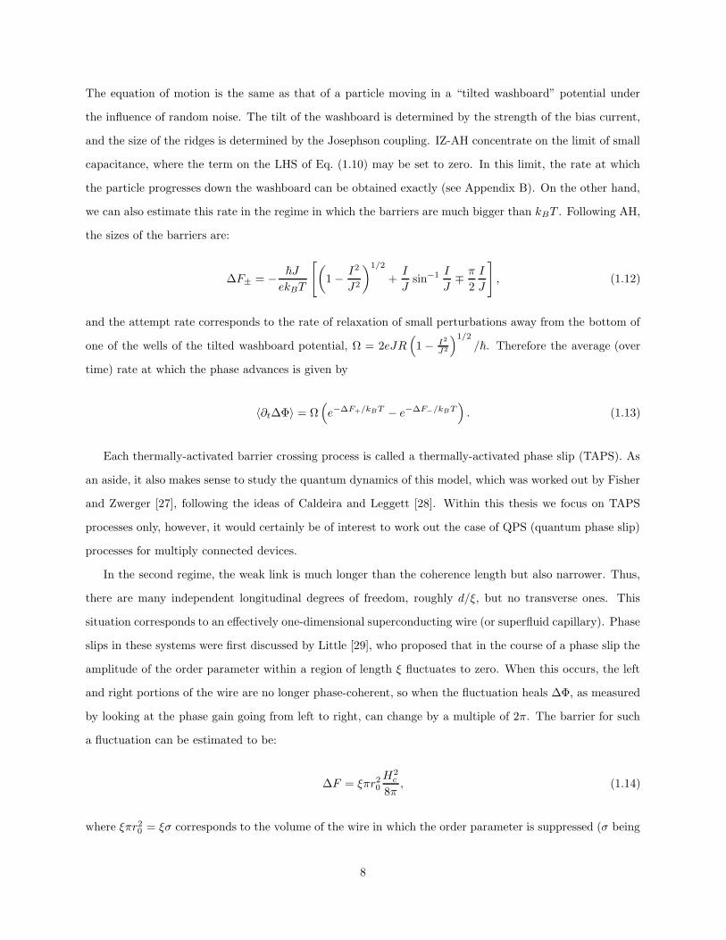
the shading scheme in Fig. 1.3. Finally, I would like to thank my fiancee, Dr. Preeti Kaur, for inspiring me

to work hard and to reach, successfully, beyond my abilities.

vi

Table of Contents

List of Tables . . . . . . . . . . . . . . . . . . . . . . . . . . . . . . . . . . . . . . . . . . . . . . ix

List of Figures . . . . . . . . . . . . . . . . . . . . . . . . . . . . . . . . . . . . . . . . . . . . . . x

List of Abbreviations . . . . . . . . . . . . . . . . . . . . . . . . . . . . . . . . . . . . . . . . . xii

Chapter 1 Introduction to phase-slip processes . . . . . . . . . . . . . . . . . . . . . . . . . 11.1 Phase coherence and topological excitations . . . . . . . . . . . . . . . . . . . . . . . . . . . . 41.2 Thermally activated phase-slips . . . . . . . . . . . . . . . . . . . . . . . . . . . . . . . . . . . 61.3 Overview of the dissertation . . . . . . . . . . . . . . . . . . . . . . . . . . . . . . . . . . . . . 9

Chapter 2 Superconducting two-nanowire devices . . . . . . . . . . . . . . . . . . . . . . . 112.1 Introduction . . . . . . . . . . . . . . . . . . . . . . . . . . . . . . . . . . . . . . . . . . . . . . 112.2 Origin of magnetoresistance oscillations . . . . . . . . . . . . . . . . . . . . . . . . . . . . . . 15

2.2.1 Device geometry . . . . . . . . . . . . . . . . . . . . . . . . . . . . . . . . . . . . . . . 152.2.2 Parametric control of the state of the wires by the leads . . . . . . . . . . . . . . . . . 152.2.3 Simple estimate of the oscillation period . . . . . . . . . . . . . . . . . . . . . . . . . . 17

2.3 Mesoscale superconducting leads . . . . . . . . . . . . . . . . . . . . . . . . . . . . . . . . . . 192.3.1 Vortex-free and vorticial regimes . . . . . . . . . . . . . . . . . . . . . . . . . . . . . . 192.3.2 Phase variation along the edge of the lead . . . . . . . . . . . . . . . . . . . . . . . . . 202.3.3 Period of magnetoresistance for leads having a rectangular strip geometry . . . . . . . 232.3.4 Bridge-lead coupling . . . . . . . . . . . . . . . . . . . . . . . . . . . . . . . . . . . . . 232.3.5 Strong nanowires . . . . . . . . . . . . . . . . . . . . . . . . . . . . . . . . . . . . . . . 25

2.4 Parallel superconducting nanowires and intrinsic resistance . . . . . . . . . . . . . . . . . . . 262.4.1 Short nanowires: Josephson junction limit . . . . . . . . . . . . . . . . . . . . . . . . . 272.4.2 Longer nanowires: LAMH regime . . . . . . . . . . . . . . . . . . . . . . . . . . . . . . 28

2.5 Connections with experiment . . . . . . . . . . . . . . . . . . . . . . . . . . . . . . . . . . . . 372.5.1 Device fabrication . . . . . . . . . . . . . . . . . . . . . . . . . . . . . . . . . . . . . . 372.5.2 Comparison between theory and experiment . . . . . . . . . . . . . . . . . . . . . . . . 38

2.6 Multi-wire devices . . . . . . . . . . . . . . . . . . . . . . . . . . . . . . . . . . . . . . . . . . 402.7 Cross currents and applications . . . . . . . . . . . . . . . . . . . . . . . . . . . . . . . . . . . 41

2.7.1 Cross current measurements with no magnetic field . . . . . . . . . . . . . . . . . . . . 432.7.2 Vorticial regime . . . . . . . . . . . . . . . . . . . . . . . . . . . . . . . . . . . . . . . . 472.7.3 Estimate of period due to magnetic fields generated by the cross current . . . . . . . . 49

2.8 Concluding remarks . . . . . . . . . . . . . . . . . . . . . . . . . . . . . . . . . . . . . . . . . 51

Chapter 3 Superflow through arrays of nanosized apertures: disorder, fluctuations,avalanches, criticality, and other stories . . . . . . . . . . . . . . . . . . . . . . . . . . . . 523.1 Introduction . . . . . . . . . . . . . . . . . . . . . . . . . . . . . . . . . . . . . . . . . . . . . . 55

3.1.1 Bulk energy . . . . . . . . . . . . . . . . . . . . . . . . . . . . . . . . . . . . . . . . . . 563.1.2 Single-aperture dynamics in the Josephson regime . . . . . . . . . . . . . . . . . . . . 603.1.3 Single-aperture dynamics in the phase slippage regime . . . . . . . . . . . . . . . . . . 61

vii

3.1.4 Summary of the model . . . . . . . . . . . . . . . . . . . . . . . . . . . . . . . . . . . . 623.2 Analysis of array dynamics in the Josephson regime . . . . . . . . . . . . . . . . . . . . . . . 633.3 Analysis of the array dynamics in the phase-slippage regime . . . . . . . . . . . . . . . . . . . 67

3.3.1 Numerical procedure . . . . . . . . . . . . . . . . . . . . . . . . . . . . . . . . . . . . . 683.3.2 Mean-field theory describing phase-slip dynamics . . . . . . . . . . . . . . . . . . . . . 693.3.3 Renormalization group analysis via ε-expansion . . . . . . . . . . . . . . . . . . . . . . 733.3.4 Pinning of charge density waves . . . . . . . . . . . . . . . . . . . . . . . . . . . . . . . 753.3.5 Soft-spin random field Ising model . . . . . . . . . . . . . . . . . . . . . . . . . . . . . 753.3.6 Connection between the random field Ising model and the present model of interacting

phase-slips . . . . . . . . . . . . . . . . . . . . . . . . . . . . . . . . . . . . . . . . . . 763.3.7 Martin-Siggia-Rose formalism . . . . . . . . . . . . . . . . . . . . . . . . . . . . . . . . 783.3.8 Saddle-point expansion . . . . . . . . . . . . . . . . . . . . . . . . . . . . . . . . . . . 783.3.9 Renormalization-group analysis . . . . . . . . . . . . . . . . . . . . . . . . . . . . . . . 813.3.10 Implications for experiment . . . . . . . . . . . . . . . . . . . . . . . . . . . . . . . . . 823.3.11 Concluding remarks . . . . . . . . . . . . . . . . . . . . . . . . . . . . . . . . . . . . . 85

Chapter 4 Conclusions . . . . . . . . . . . . . . . . . . . . . . . . . . . . . . . . . . . . . . . . 87

Appendix A Physical Scales . . . . . . . . . . . . . . . . . . . . . . . . . . . . . . . . . . . . 88

Appendix B Ambegaokar-Halperin formula for resistance of a dampedJosephson junction . . . . . . . . . . . . . . . . . . . . . . . . . . . . . . . . . . . . . . . . . 89

Appendix C LA-MH theory for a single bridge . . . . . . . . . . . . . . . . . . . . . . . . . 90

Appendix D Josephson effect in a single aperture . . . . . . . . . . . . . . . . . . . . . . . 94D.1 Partition function . . . . . . . . . . . . . . . . . . . . . . . . . . . . . . . . . . . . . . . . . . . 95D.2 Electrostatic approach to partition function . . . . . . . . . . . . . . . . . . . . . . . . . . . . 97D.3 Supercurrent . . . . . . . . . . . . . . . . . . . . . . . . . . . . . . . . . . . . . . . . . . . . . 97D.4 Results . . . . . . . . . . . . . . . . . . . . . . . . . . . . . . . . . . . . . . . . . . . . . . . . . 98

Appendix E Avalanche size scaling and other critical exponents in mean-field-theory . . 99E.1 Avalanche size distribution . . . . . . . . . . . . . . . . . . . . . . . . . . . . . . . . . . . . . 99E.2 Mean-field-theory in the vicinity of criticality . . . . . . . . . . . . . . . . . . . . . . . . . . . 101

E.2.1 Mean-field-theory in the vicinity of σc . . . . . . . . . . . . . . . . . . . . . . . . . . . 102E.2.2 Mean-field-theory for σ < σc . . . . . . . . . . . . . . . . . . . . . . . . . . . . . . . . 103E.2.3 Mean-field equations for the critical line . . . . . . . . . . . . . . . . . . . . . . . . . . 104

Appendix F The renormalization group transformation of the long-rangesoft-spin RFIM . . . . . . . . . . . . . . . . . . . . . . . . . . . . . . . . . . . . . . . . . . . 105

References . . . . . . . . . . . . . . . . . . . . . . . . . . . . . . . . . . . . . . . . . . . . . . . . 108

Author’s Biography . . . . . . . . . . . . . . . . . . . . . . . . . . . . . . . . . . . . . . . . . . 112

viii

List of Tables

2.1 Comparison between measured and theoretical magnetoresistance periods . . . . . . . . . . . 39

ix

List of Figures

1.1 Schematic depiction of vortex pairs and vortex loops . . . . . . . . . . . . . . . . . . . . . . . 51.2 Circuit diagram of a resistively and capacitively shunted Josephson junction . . . . . . . . . . 71.3 Schematic depiction of a half-loop vortex line crossing the aperture . . . . . . . . . . . . . . . 9

2.1 Schematic depiction of the superconducting phase gradiometer and an SEM micrograph oftwo metal coated DNA molecules . . . . . . . . . . . . . . . . . . . . . . . . . . . . . . . . . . 13

2.2 Geometry of the two-wire device, showing the dimensions . . . . . . . . . . . . . . . . . . . . 132.3 Phase accumulations around the gradiometer . . . . . . . . . . . . . . . . . . . . . . . . . . . 152.4 Current profile in a long superconducting strip . . . . . . . . . . . . . . . . . . . . . . . . . . 182.5 Phase profile in the leads in the vicinity of the trench . . . . . . . . . . . . . . . . . . . . . . 222.6 Phase profile on the x = −L (i.e. short) edge of the strip . . . . . . . . . . . . . . . . . . . . . 242.7 Sample 219-4: Experimental data and theoretical fits to the Josephson junction model . . . . 292.8 Parallel and sequential phase slip processes . . . . . . . . . . . . . . . . . . . . . . . . . . . . 292.9 Diagram depicting the stable, metastable, and saddle-point states of the two wire system with

δ = nπ . . . . . . . . . . . . . . . . . . . . . . . . . . . . . . . . . . . . . . . . . . . . . . . . . 332.10 Diagram depicting the stable, metastable, and saddle-point states of the two wire system with

δ = (n+ 1/2)π . . . . . . . . . . . . . . . . . . . . . . . . . . . . . . . . . . . . . . . . . . . . 352.11 Amplitude of the order parameter at the end of a wire, as a function of its value at the mid-point 372.12 Current vs. end-to-end phase accumulation for superconducting wires of various lengths . . . 382.13 Sample 219-4: Resistance vs. temperature curves . . . . . . . . . . . . . . . . . . . . . . . . . 392.14 Sample 930-1: Resistance vs. temperature curves . . . . . . . . . . . . . . . . . . . . . . . . . 402.15 Effective single junction critical current for a multi-junction array, as a function of δ . . . . . 412.16 Schematic of the DNA-templated two-nanowire device for cross-current measurements . . . . 422.17 Resistance vs. temperature for various cross currents . . . . . . . . . . . . . . . . . . . . . . . 432.18 Resistance vs. cross-current data and fits . . . . . . . . . . . . . . . . . . . . . . . . . . . . . . 442.19 Cross-current period in the resistance oscillation vs. temperature . . . . . . . . . . . . . . . . 452.20 Resistance vs. magnetic field . . . . . . . . . . . . . . . . . . . . . . . . . . . . . . . . . . . . 462.21 Resistance vs. cross-current measured at various values of the field . . . . . . . . . . . . . . . 462.22 Inverse of the oscillation period vs. field . . . . . . . . . . . . . . . . . . . . . . . . . . . . . . 482.23 Geometry used to compute the effects of generated magnetic field . . . . . . . . . . . . . . . . 50

3.1 Schematic of the model system. . . . . . . . . . . . . . . . . . . . . . . . . . . . . . . . . . . . 543.2 Schematic diagram of the (electrostatic) boundary value problem . . . . . . . . . . . . . . . . 583.3 Effective Josephson coupling strength, as a function of the number of apertures . . . . . . . . 663.4 Current vs. time comparison of mean-field theory and numerics . . . . . . . . . . . . . . . . . 693.5 Graphical solution of the MFT equation . . . . . . . . . . . . . . . . . . . . . . . . . . . . . . 703.6 Phase diagram, showing avalanching and non-avalanching regimes of the phase-slip dynamics 713.7 Line of critical points in the control phase twist–disorder plane . . . . . . . . . . . . . . . . . 723.8 Amplitude of the oscillation of the current and the drop in current caused by an SWA . . . . 743.9 Vertices associated with the effective action, Eq. (3.71). . . . . . . . . . . . . . . . . . . . . . 813.10 Feynman diagrams for the renormalization group at one loop order. . . . . . . . . . . . . . . 81

x

3.11 Effect of array edges on amplitude of current oscillations . . . . . . . . . . . . . . . . . . . . . 85

C.1 “Mechanical potential” U(u = f 2) at an intermediate value of the dimensionless current . . . 91C.2 Squared amplitude u of the order parameter . . . . . . . . . . . . . . . . . . . . . . . . . . . . 93

xi

List of Abbreviations

GL V. L. Ginzburg and L. D. Landau [1]

BCS J. Bardeen, L. Cooper, R. Schriffer [2]

MQC Macroscopic Quantum Coherence

ODLRO Off Diagonal Long Range Order

IZ-AH Y. M. Ivanchenko, L. A. Zil’berman [3, 4], V. Ambegaokar, and B. I. Halperin [5]

LAMH J. S. Langer, V. Ambegaokar [6], D .E. McCumber, and B. I. Halperin [7]

CDW Charge Density Wave

RFIM Random Field Ising Model

SWA System-Wide Avalanche

MSR P. C. Martin, E. D. Siggia, and H. A. Rose [88]

xii

Chapter 1

Introduction to phase-slip processes

In 1911 in the laboratory of Heike Kamerlingh Onnes it was discovered that when mercury is cooled to

a temperature below approximately 4.2 K its resistivity abruptly vanishes. The drop in the resistivity is

associated with a discontinuity in the heat capacity, indicating the formation of a new state of matter – the

superconducting state. In 1933 Walther Meissner and Robert Ochsenfeld [8] discovered that, in addition

to losing electrical resistance, superconductors are also perfect diamagnets in that they completely expel

magnetic fields, a property that has become known as the Meissner effect.

The first phenomenological model of superconductivity was proposed by Fritz and Heinz London [9]. They

postulated that within a superconductor there are two types of electrons: normal and superconducting. The

DC electrical properties would be determined by the superconducting electrons, which would have zero

electrical resistance and also the following constitutive property:

A = −4π

cλ2j, (1.1)

where A is the electromagnetic vector potential, j is the charge current density, and λ ≡√m∗c2/4πnse2

sets the scale for the magnetic field penetration depth (m∗ is the mass of the carrier and ns is the number

density of the superconducting carriers). Equation 1.1 relies on a special choice of gauge, called the London

gauge, in which A at the edges of the superconducting sample is parallel to those edges. Further, Eq. 1.1,

arises as the result of choosing a zero value for the integration constant in Newton’s equation of motion

for the electron, which corresponds to the absence of a magnetic field deep within the superconductor. An

important consequence of this property is the perfect expulsion of magnetic fields from bulk superconductors,

i.e. perfect diamagnetism.

In 1950 Vitaly Lazarevich Ginzburg and Lev Davidovich Landau (GL) proposed a more refined phe-

nomenological model of superconductivity that better captured the quantum nature of the superconducting

state [1]. Their model is a model of spontaneous symmetry breaking that occurs at the superconducting

phase transition. The superconducting state is described by a complex scalar field ψ that acquires a nonzero

1

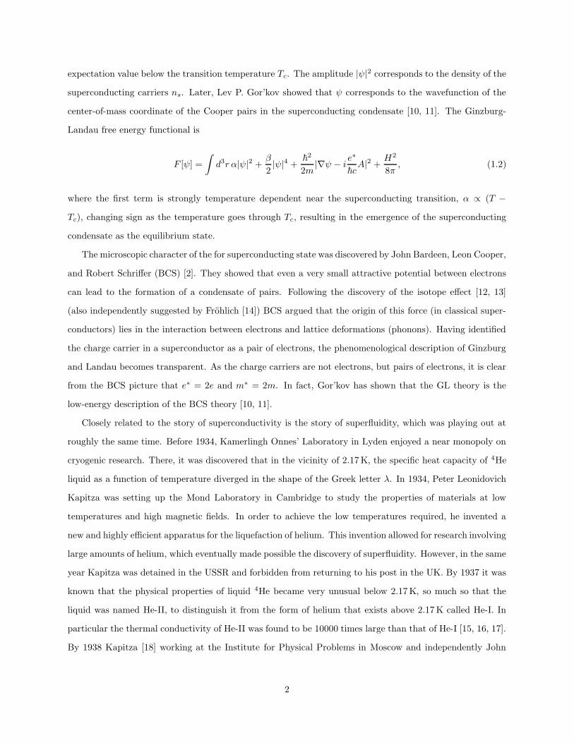
expectation value below the transition temperature Tc. The amplitude |ψ|2 corresponds to the density of the

superconducting carriers ns. Later, Lev P. Gor’kov showed that ψ corresponds to the wavefunction of the

center-of-mass coordinate of the Cooper pairs in the superconducting condensate [10, 11]. The Ginzburg-

Landau free energy functional is

F [ψ] =

∫d3r α|ψ|2 +

β

2|ψ|4 +

~2

2m|∇ψ − i e

∗

~cA|2 +

H2

8π, (1.2)

where the first term is strongly temperature dependent near the superconducting transition, α ∝ (T −

Tc), changing sign as the temperature goes through Tc, resulting in the emergence of the superconducting

condensate as the equilibrium state.

The microscopic character of the for superconducting state was discovered by John Bardeen, Leon Cooper,

and Robert Schriffer (BCS) [2]. They showed that even a very small attractive potential between electrons

can lead to the formation of a condensate of pairs. Following the discovery of the isotope effect [12, 13]

(also independently suggested by Frohlich [14]) BCS argued that the origin of this force (in classical super-

conductors) lies in the interaction between electrons and lattice deformations (phonons). Having identified

the charge carrier in a superconductor as a pair of electrons, the phenomenological description of Ginzburg

and Landau becomes transparent. As the charge carriers are not electrons, but pairs of electrons, it is clear

from the BCS picture that e∗ = 2e and m∗ = 2m. In fact, Gor’kov has shown that the GL theory is the

low-energy description of the BCS theory [10, 11].

Closely related to the story of superconductivity is the story of superfluidity, which was playing out at

roughly the same time. Before 1934, Kamerlingh Onnes’ Laboratory in Lyden enjoyed a near monopoly on

cryogenic research. There, it was discovered that in the vicinity of 2.17 K, the specific heat capacity of 4He

liquid as a function of temperature diverged in the shape of the Greek letter λ. In 1934, Peter Leonidovich

Kapitza was setting up the Mond Laboratory in Cambridge to study the properties of materials at low

temperatures and high magnetic fields. In order to achieve the low temperatures required, he invented a

new and highly efficient apparatus for the liquefaction of helium. This invention allowed for research involving

large amounts of helium, which eventually made possible the discovery of superfluidity. However, in the same

year Kapitza was detained in the USSR and forbidden from returning to his post in the UK. By 1937 it was

known that the physical properties of liquid 4He became very unusual below 2.17 K, so much so that the

liquid was named He-II, to distinguish it from the form of helium that exists above 2.17 K called He-I. In

particular the thermal conductivity of He-II was found to be 10000 times large than that of He-I [15, 16, 17].

By 1938 Kapitza [18] working at the Institute for Physical Problems in Moscow and independently John

2

F. Allen and A. D. Misener [19] working at the Mond Laboratory in Cambridge discovered a most striking

phenomenon: the new “form” of Helium seemed to have vanishingly small viscosity, and was thus able to flow

through capillaries without resistance (or to leak out of a container that had the tiniest hole), a phenomenon

that Kapitza called superfluidity. The investigation of the anomalously high thermal conductivity of He-II

led to the discovery of the fountain effect [20]. The lack of viscosity in He-II was associated with the lack of

resistance in superconductors, and thus was named superfluidity [21].

According to Pitaevskii, one of the first practical application of superfluidity arose in 1938, when Landau

was arrested “as a result of an outrageous and false (but typical for those days) accusations of espionage

and sabotage” [22]. Peter Kapitza, who at the time was the head of the Institute for Physical Problems in

Moscow, used superfluidity as an excuse in his fight to save Landau. A year before Landau’s arrest, Kapitza

had arranged for Landau to move to Moscow, which undoubtedly delayed the arrest. On the day of the

arrest, Kapitza wrote a letter to J. V. Stalin, the Secretary General of the Communist Party, on Landau’s

behalf. However, neither Kapitza’s letter nor one from Niels Bohr had the desired effect. Next, Kapitza

wrote a letter to V. M. Molotov, the second highest political figure after Stalin, demanding that he needed a

good theorist like Landau to help him write a paper on the properties of superfluid Helium. This approach

worked and Landau was released.

To explain the superfluid effect, Landau suggested the following phenomenological criterion [23]: excita-

tions in a fluid may be generated only when the phase velocity of the excitation exceeds the flow velocity of

the fluid. Therefore, Landau defined the critical velocity, vc, as the phase velocity of the slowest excitation:

vc = minε(p)

p, (1.3)

where p is the momentum and ε(p) the energy of the excitation. If vc is nonzero then the fluid is a superfluid

and exhibits dissipationless flow at velocities smaller than vc. If vc is exceeded then elementary excitations

start to be created by the flow, resulting in viscous drag on the fluid. Landau further developed the theory of

two-fluid (quasi-)hydrodynamics describing the quantum superfluid component and the normal component

and their interactions.

A useful description of superfluidity, which will be the basis for further calculations within this thesis, was

proposed independently by Gross [24, 25] and Pitaevskii [26]. Consider the many-body Heisenberg equation

of motion for the field operator Ψ(r, t) =∑

α ψα(r, t)aα, where the aα’s are the annihilation operators for

3

the single-particle wave functions ψα(r). This equation of motion reads

i~∂

∂tΨ(r, t) = [Ψ, H ] (1.4)

=

[−~

2∇2r

2m+ Vext(r) +

∫dr′ |Ψ(r′, t)|2V (r − r′)

]Ψ(r, t), (1.5)

where Vext(r) is the external or confining potential and V (r − r′) is the two-particle interaction potential.

Replacing the field operator Ψ by its expectation value Φ(r, t) = 〈Ψ(r, t)〉 we obtain the mean-field equation

known as the Gross-Pitaevskii equation:

i~∂

∂tΦ(r, t) =

[−~

2∇2

2m+ Vext(r) + g|Φ(r, t)|2

]Φ(r, t), (1.6)

where we have also replaced the two-particle potential by the point contact interaction V (r′−r) = gδ(r′−r).

Here, Φ plays the role of an order parameter. Strictly speaking, the Gross-Pitaevskii description is only

correct at zero temperature, when there are no excitations present, and even then it neglects correlation

effects. In this thesis we concentrate only on the properties of the analogous static equation, where the

left-hand-side is set to zero.

1.1 Phase coherence and topological excitations

The key feature of both superfluids and superconductors is their so-called macroscopic quantum coherence

(MQC), which is a direct consequence of their off diagonal long range order (ODLRO). MQC implies that

the amplitude and the phase of the order parameter ψ(r) (i.e. the wavefunction of superfluid atoms for

the case of superfluids, or the center-of-mass of the Cooper pairs for the case of superconductors) are both

sufficiently stiff that the two-point correlator is always nonzero:

〈ψ†(r)ψ(0)〉 6= 0, (1.7)

and approaches some finite value ns as r → ∞ called the condensate fraction 1. Therefore, it is reasonable

to ask how the order parameter changes as one follows a closed-loop? Assuming that we choose a loop

where the amplitude of the order parameter is always non-zero, the single valuedness of the order parameter

1In two dimensions, for T < TKTB , this correlator falls off algebraically with separation, resulting in superfluidity with nolong range order.

4

2-D 3-D

edge edge

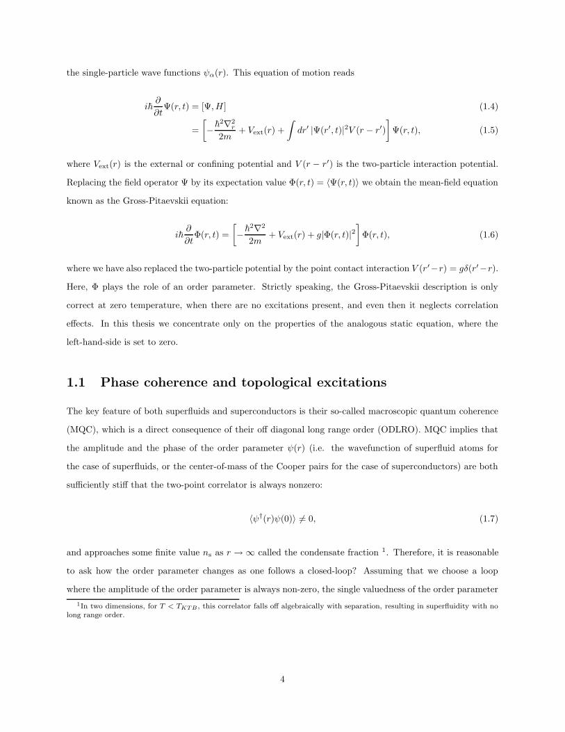
Figure 1.1: Schematic depiction of the formation of vortex pairs and vortex loops. The stars depict thefluctuation from which the vortices are born. Top row: formation of vortex pairs (left) and a vortex loop(right) in bulk superfluid. Bottom row: formation of a single vortex (left) and a vortex half-loop (right) ata superfluid edge.

implies that the phase gain around the loop is a multiple of 2π:

∮∇φ · dl = 2πn, n ∈ Z. (1.8)

In other words, as the order parameter is a complex scalar, the first homotopy group of the mapping between

the space of nonzero order parameters and closed loops is Z. Therefore, each closed loop encircles an integer

number of quantized vortices that pass through it. Furthermore, in order to change the number of vortices

within such a closed loop, somewhere along the loop the order-parameter must temporarily become zero.

These arguments imply that in two spatial dimensions, within the bulk superfluid or superconductor,

vortices must be born in pairs with partners of opposite vorticity, which may later separate. For the case of

three dimensions vortices must be born as vortex line that closes on itself, which may later expand in space.

A vortex line is a line along which the amplitude of the order parameter is zero, and if we integrate the phase

gain along a contour that winds around the vortex line exactly once the result is a multiple of 2π associated

with the vorticity of the vortex line. The formation of vortex-anti-vortex pairs and closed vortex lines is

illustrated in the top row of Fig. 1.1. The situation is different if the superfluid has a boundary. In two

dimensions isolated vortices may be born directly on a boundary, while in three or more dimensions vortex

lines in the shape of half-loops may spontaneously emerge, the vortex line being anchored to the boundary

at both ends of the half-loop. The formation of isolated vortices and vortex half-loops is illustrated in the

bottom row of Fig. 1.1.

Before proceeding to describe phase-slips, we make some remarks regarding the structure of vortices and

vortex-lines. Within the context of this thesis, we shall confine ourselves to the structure and properties

5

of vortices as obtained from the GL equation. We assume that the temperature is sufficiently below the

transition temperature that order parameter fluctuations may be ignored. For the case of neutral superfluids,

ξ is the only length-scale, and it determines the size of the vortex core, i.e. the size of the region where the

order parameter amplitude is suppressed. For the case of superconductors, there are two lengths-scales, ξ

and λ, which determine the vortex structure. If λ < ξ then vortices are unstable. On the other hand if

λ > ξ then vortices are stable. For this case, ξ again determines the size of the core, whereas λ determines

the size of the region of flux-penetration associated with the vortex.

1.2 Thermally activated phase-slips

We shall specialize to geometries having two bulk superfluids or superconductors connected by one or more

weak links. The weak links that we shall consider are either small apertures in a thin membrane separating the

two bulk superfluids or narrow superconducting bridges or wires connecting two large bulk superconductors.

We shall briefly discuss the properties of a single weak link and then move on to the main focus: devices

that have multiple weak links. Consider a single weak-link device with a small current I flowing through

the weak link between the two bulks. Assign ΦL and ΦR to be the phases of the left and right bulk. We

would like to describe the dynamics of the phase difference ∆Φ = ΦR − ΦL. The weak link is called weak

because it allows for so-called phase-slip process. In a phase-slip process the order parameter amplitude is

completely suppressed within the weak link, by either a thermal or a quantum fluctuation, and, therefore,

∆Φ changes by a multiple of 2π after the process is complete.

We shall describe the weak links by length d, and radius r0. Throughout this thesis, we focus on the

case of devices much smaller than λ, and therefore we ignore the lengthscale associated with λ. Within this

regime we may order the lengthscales in the following four ways:

1. ξ & d, 2r0 — The weak link functions as a Josephson junction.

2. d ξ & 2r0 — The weak link functions as a one-dimensional superconducting wire.

3. 2r0 ξ & d — The weak link functions as a wide Josephson junction.

4. 2r0, d ξ — The weak link functions as a wide wire.

In the first regime the size of the weak link (both d and r0) is smaller than ξ, therefore there cannot

be any additional degrees of freedom associated with the weak link, except for the phase difference between

the two bulk superfluids, ∆Φ. This situation exactly corresponds to that of a Josephson junction. Here, the

GL equation within the weak link is dominated by the gradient term and there is only one stable solution

for each value of ∆Φ. The thermodynamics of a Josephson junction shunted by a capacitor and a resistor

6

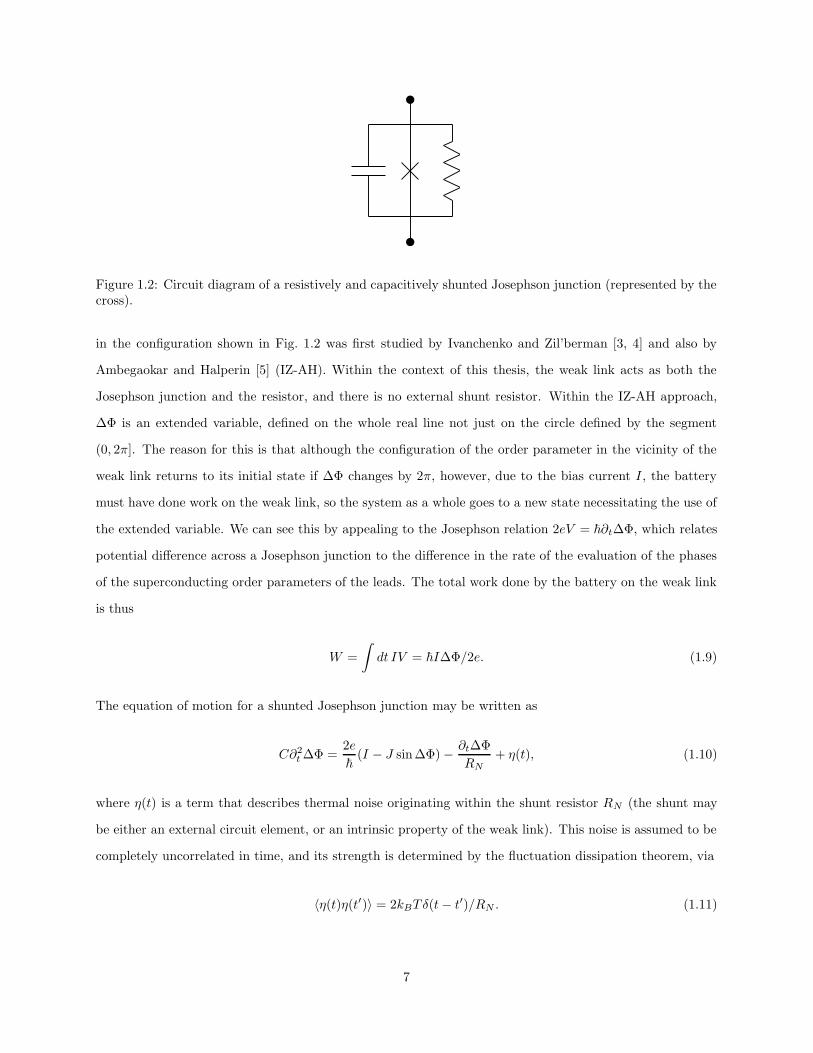
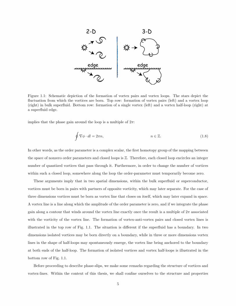
Figure 1.2: Circuit diagram of a resistively and capacitively shunted Josephson junction (represented by thecross).

in the configuration shown in Fig. 1.2 was first studied by Ivanchenko and Zil’berman [3, 4] and also by

Ambegaokar and Halperin [5] (IZ-AH). Within the context of this thesis, the weak link acts as both the

Josephson junction and the resistor, and there is no external shunt resistor. Within the IZ-AH approach,

∆Φ is an extended variable, defined on the whole real line not just on the circle defined by the segment

(0, 2π]. The reason for this is that although the configuration of the order parameter in the vicinity of the

weak link returns to its initial state if ∆Φ changes by 2π, however, due to the bias current I , the battery

must have done work on the weak link, so the system as a whole goes to a new state necessitating the use of

the extended variable. We can see this by appealing to the Josephson relation 2eV = ~∂t∆Φ, which relates

potential difference across a Josephson junction to the difference in the rate of the evaluation of the phases

of the superconducting order parameters of the leads. The total work done by the battery on the weak link

is thus

W =

∫dt IV = ~I∆Φ/2e. (1.9)

The equation of motion for a shunted Josephson junction may be written as

C∂2t ∆Φ =

2e

~(I − J sin ∆Φ)− ∂t∆Φ

RN+ η(t), (1.10)

where η(t) is a term that describes thermal noise originating within the shunt resistor RN (the shunt may

be either an external circuit element, or an intrinsic property of the weak link). This noise is assumed to be

completely uncorrelated in time, and its strength is determined by the fluctuation dissipation theorem, via

〈η(t)η(t′)〉 = 2kBTδ(t− t′)/RN . (1.11)

7

The equation of motion is the same as that of a particle moving in a “tilted washboard” potential under

the influence of random noise. The tilt of the washboard is determined by the strength of the bias current,

and the size of the ridges is determined by the Josephson coupling. IZ-AH concentrate on the limit of small

capacitance, where the term on the LHS of Eq. (1.10) may be set to zero. In this limit, the rate at which

the particle progresses down the washboard can be obtained exactly (see Appendix B). On the other hand,

we can also estimate this rate in the regime in which the barriers are much bigger than kBT . Following AH,

the sizes of the barriers are:

∆F± = − ~J

ekBT

[(1− I2

J2

)1/2

+I

Jsin−1 I

J∓ π

2

I

J

], (1.12)

and the attempt rate corresponds to the rate of relaxation of small perturbations away from the bottom of

one of the wells of the tilted washboard potential, Ω = 2eJR(

1− I2

J2

)1/2

/~. Therefore the average (over

time) rate at which the phase advances is given by

〈∂t∆Φ〉 = Ω(e−∆F+/kBT − e−∆F−/kBT

). (1.13)

Each thermally-activated barrier crossing process is called a thermally-activated phase slip (TAPS). As

an aside, it also makes sense to study the quantum dynamics of this model, which was worked out by Fisher

and Zwerger [27], following the ideas of Caldeira and Leggett [28]. Within this thesis we focus on TAPS

processes only, however, it would certainly be of interest to work out the case of QPS (quantum phase slip)

processes for multiply connected devices.

In the second regime, the weak link is much longer than the coherence length but also narrower. Thus,

there are many independent longitudinal degrees of freedom, roughly d/ξ, but no transverse ones. This

situation corresponds to an effectively one-dimensional superconducting wire (or superfluid capillary). Phase

slips in these systems were first discussed by Little [29], who proposed that in the course of a phase slip the

amplitude of the order parameter within a region of length ξ fluctuates to zero. When this occurs, the left

and right portions of the wire are no longer phase-coherent, so when the fluctuation heals ∆Φ, as measured

by looking at the phase gain going from left to right, can change by a multiple of 2π. The barrier for such

a fluctuation can be estimated to be:

∆F = ξπr20H2

c

8π, (1.14)

where ξπr20 = ξσ corresponds to the volume of the wire in which the order parameter is suppressed (σ being

8

1 2 3 4 5 6

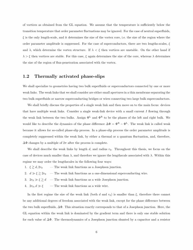
Figure 1.3: Schematic depiction of a half-loop vortex line crossing the aperture. The half-loop is nucleatedin slice 1, the end points move around the aperture and rejoin in slice 6. Phase gain going from left to rightreservoir differs by 2π depending on whether the trajectory goes through the blue or white region.

the cross-sectional area) and H2c /8π is the condensation energy per unit volume. The rate of phase slips

follows the Arrhenius law Γ ∼ exp(−∆F/kBT ). Furthermore, due to the bias current I flowing through the

weak link, the barrier for phase slips that add or subtract 2π phase differences differ. Langer and Ambegaokar

(LA) further extended Little’s proposal by computing the free energy barrier for the one-dimensional GL

model of the wire [6] (see Appendix C). McCumber compared the current- and voltage-biased cases [30].

Finally, McCumber and Halperin computed the pre-exponential factor to find the rate at which phase slips

occur [7].

The third regime corresponds to the situation described by Anderson [31]. In this setting, there are many

transverse degrees of freedom. Phase slippage occurs by the nucleation of a half-loop line vortex that sweeps

across the aperture as indicated in Fig. 1.3. The computation of the barrier to phase-slippage in this regime

is much more complicated, and is dependent on the properties of the walls of the aperture.

The fourth regime is similar to the third one, in that phase-slips occur via crossing of half-loop vortex lines.

This regime will feature prominently in Chapter 3; however, we shall consider only a simple deterministic

model of the superflow through such an aperture, in which a phase slip occurs once the supervelocity exceeds

an aperture-dependent critical velocity.

1.3 Overview of the dissertation

The main goal of this thesis is to examine properties of the dynamics of multiply-connected superfluid

and superconducting systems. The thesis is split into two main parts. In Chapter 2 we concentrate on

a system studied experimentally by David S. Hopkins and Alexey Bezryadin. It is composed of two bulk

superconductors connected by a parallel pair of superconducting wires. We have developed a detailed model

of this system and computed the barriers (and, consequently, rates for phase slips) in the various wires and

how these depend on currents and magnetic fields applied to the bulk superconductors. In Chapter 3, we

9

describe our work inspired by the experiments of Yuki Sato, Aditya Joshi, and Richard Packard on the

superflow of helium through an array of nanosized apertures in a thin membrane. We find that, due to the

coupling between the superflows in the various apertures, this system can display a wide variety of dynamic

processes.

10

Chapter 2

Superconducting two-nanowire

devices

In this Chapter a theory describing the operation of a superconducting nanowire quantum interference device

(NQUID) is presented. The device consists of a pair of thin-film superconducting leads connected by a pair

of topologically parallel ultra-narrow superconducting wires. It exhibits intrinsic electrical resistance, due to

thermally-activated dissipative fluctuations of the superconducting order parameter. Attention is given to

the dependence of this resistance on the strength of an externally applied magnetic field aligned perpendic-

ular to the leads, for lead dimensions such that there is essentially complete and uniform penetration of the

leads by the magnetic field. This regime, in which at least one of the lead dimensions—length or width—lies

between the superconducting coherence and penetration lengths, is referred to as the mesoscopic regime. The

magnetic field causes a pronounced oscillation of the device resistance, with a period not dominated by the

Aharonov-Bohm effect through the area enclosed by the wires and the film edges but, rather, in terms of the

geometry of the leads, in contrast to the well-known Little-Parks resistance of thin-walled superconducting

cylinders. A detailed theory, encompassing this phenomenology quantitatively, is developed through exten-

sions, to the setting of parallel superconducting wires, of the Ivanchenko-Zil’berman-Ambegaokar-Halperin

theory of intrinsic resistive fluctuations in a current-biased Josephson junctions and the Langer-Ambegaokar-

McCumber-Halperin theory of intrinsic resistive fluctuations in superconducting wires. In particular, it is

demonstrated that via the resistance of the NQUID, the wires act as a probe of spatial variations in the

superconducting order parameter along the perimeter of each lead: in essence, a superconducting phase

gradiometer.

This work was done in collaboration with D. S. Hopkins, A. Bezryadin, and P. M. Goldbart.

2.1 Introduction

The Little-Parks effect concerns the electrical resistance of a thin cylindrically-shaped superconducting film

and, specifically, the dependence of this resistance on the magnetic flux threading the cylinder [32, 33, 34].

It is found that the resistance is a periodic function of the magnetic field, with period inversely proportional

11

to the cross-sectional area of the cylinder. Similarly, in a DC SQUID, the critical value of the supercurrent

is periodic in magnetic field, with period inversely proportional to the area enclosed by the SQUID ring [34].

In this Chapter, we consider a mesoscopic analog of a DC SQUID. The analog consists of a device

composed of a thin superconducting film patterned into two mesoscopic leads that are connected by a pair

of (topologically) parallel, short, weak, superconducting wires. Thus, we refer to the device as an NQUID

(superconducting nanowire quantum interference device). The only restriction that we place on the wires of

the device is that they be thin enough for the order parameter to be taken as constant over each cross-section

of a wire, varying only along the wire length. In principle, this condition of one-dimensionality is satisfied

if the wire is much thinner than the superconducting coherence length ξ. In practice, it is approximately

satisfied provided the wire diameter d is smaller than 4.4 ξ [35]. For thicker wires, vortices can exist inside

the wires, and such wires may not be assumed to be one dimensional.

By the term mesoscopic we are characterizing phenomena that occur on length-scales larger than the

superconducting coherence length ξ but smaller than the electromagnetic penetration depth λ⊥ associated

with magnetic fields applied perpendicular to the superconducting film. We shall call a lead mesoscopic

if at least one of its two long dimensions is in the mesoscopic regime; the other dimension may be either

mesoscopic or macroscopic. Thus, a weak magnetic field applied perpendicular to a mesoscopic lead will

penetrate the lead without appreciable attenuation and without driving the lead from the homogeneous

superconducting state to the Abrikosov vortex state. This is similar to the regime of operation of super-

conducting wire networks; see e.g., Ref. [36, 37]. The nanowires connecting the two leads are taken to be

topologically parallel (i.e. parallel in the sense of electrical circuitry): these nanowires and edges of the leads

define a closed geometrical contour, which will be referred to as the Aharonov-Bohm (AB) contour. In our

approach, the nanowires are considered to be links sufficiently weak that any effects of the nanowires on the

superconductivity in the leads can be safely ignored.

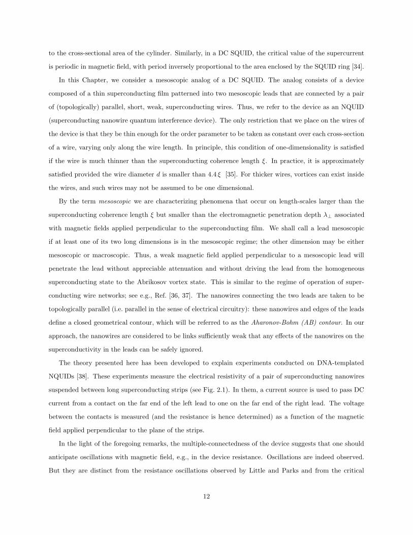
The theory presented here has been developed to explain experiments conducted on DNA-templated

NQUIDs [38]. These experiments measure the electrical resistivity of a pair of superconducting nanowires

suspended between long superconducting strips (see Fig. 2.1). In them, a current source is used to pass DC

current from a contact on the far end of the left lead to one on the far end of the right lead. The voltage

between the contacts is measured (and the resistance is hence determined) as a function of the magnetic

field applied perpendicular to the plane of the strips.

In the light of the foregoing remarks, the multiple-connectedness of the device suggests that one should

anticipate oscillations with magnetic field, e.g., in the device resistance. Oscillations are indeed observed.

But they are distinct from the resistance oscillations observed by Little and Parks and from the critical

12

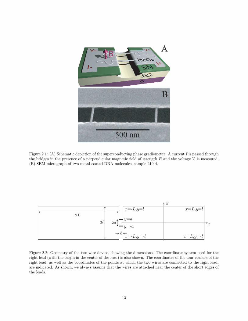
Figure 2.1: (A) Schematic depiction of the superconducting phase gradiometer. A current I is passed throughthe bridges in the presence of a perpendicular magnetic field of strength B and the voltage V is measured.(B) SEM micrograph of two metal coated DNA molecules, sample 219-4.

a

b

l

L

x=-L,y=l

x=-L,y=-l

x=L,y=l

x=L,y=-l

x

y

y=-a

y=a

Figure 2.2: Geometry of the two-wire device, showing the dimensions. The coordinate system used for theright lead (with the origin in the center of the lead) is also shown. The coordinates of the four corners of theright lead, as well as the coordinates of the points at which the two wires are connected to the right lead,are indicated. As shown, we always assume that the wires are attached near the center of the short edges ofthe leads.

13

current oscillations observed in SQUID rings. What distinguishes the resistance oscillations reported in

Ref. [38] from those found, e.g., by Little and Parks? First, the most notable aspect of these oscillations

is the value of their period. In the Little-Parks type of experiment, the period is given by Φ0/2ab, where

Φ0(≡ hc/2e) is the superconducting flux quantum, 2a is the bridge separation, and b is the bridge length,

i.e., the superconducting flux quantum divided by the area of the AB contour (see Fig. 2.2). In a high-

magnetic-field regime, such periodic behavior is indeed observed experimentally, with the length of the

period somewhat shorter but of the same order of magnitude as in the AB effect [38]. However, in a low-

magnetic-field regime, the observed period is appreciably smaller (in fact by almost two orders of magnitude

for our device geometry). Second, because the resistance is caused by thermal phase fluctuations (i.e. phase

slips) in very narrow wires, the oscillations are observable over a wide range of temperatures (∼ 1 K). Third,

the Little-Parks resistance is wholly ascribed to a rigid shift of the R(T ) curve with magnetic field, as Tc

oscillates. In contrast, in our system we observe a periodic broadening of the transition (instead of the

Little-Parks—type rigid shift) with magnetic field. Our theory explains quantitatively this broadening via

the modulation of the barrier heights for phase slips of the superconducting order parameter in the nanowires.

In the experiment, the sample is cooled in zero magnetic field, and the field is then slowly increased

while the resistance is measured. At a sample-dependent field (∼ 5 mT) the behavior switches sharply from

a low-field to a high-field regime. If the high-field regime is not reached before the magnetic field is swept

back, the low-field resistance curve is reproduced. However, once the high-field regime has been reached,

the sweeping back of the field reveals phase shifts and hysteresis in the R(B) curve. The experiments [38]

mainly address rectangular leads that have one mesoscopic and one macroscopic dimension. Therefore, we

shall concentrate on such strip geometries. We shall, however, also discuss how to extend our approach to

generic (mesoscopic) lead shapes. We note in passing that efficient numerical methods, such as the boundary

element method (BEM) [39], are available for solving the corresponding Laplace problems.

This chapter is arranged as follows. In Section 2.2 we construct a basic picture for the period of the

magnetoresistance oscillations of the two-wire device, which shows how the mesoscopic size of the leads

accounts for the anomalously short magnetoresistance period in the low-field regime. In Section 2.3 we

concentrate on the properties of mesoscopic leads with regard to their response to an applied magnetic field,

and in Section 2.4 we extend the LAMH model to take into account the inter-wire coupling through the

leads. Analytical expressions are derived for the short- and long-wire limits, whilst a numerical procedure is

described for the general case. The predictions of the model are compared with data from our experiment in

Section 2.5, and we give some concluding remarks in Section 2.8. Certain technical components are relegated

to the appendix, as is the analysis of example multiwire devices.

14

µ1,L R

!µ2,L R

!

0

2¼

±2 1,L

!

±2 1,R

!-

µ2,L R

!

-

1R 1R2R2L1L

µ1,L R

!

±2

1,R

!

±2

1,L

!

(a) (b)

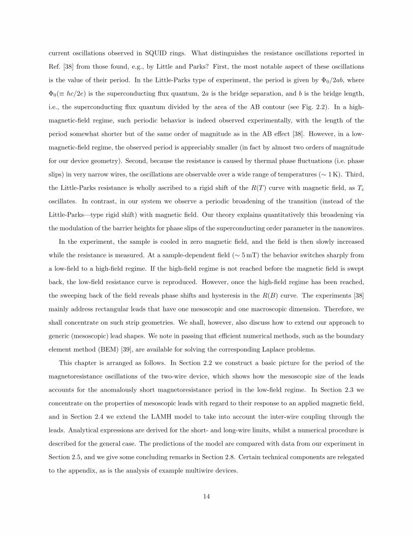
Figure 2.3: Phase accumulations around the gradiometer: (a) Close-up of the two nanowires and the leads.The top (bottom) thick arrow represents the integration contour for determining the phase accumulationθ1,L←R (θ2,L←R) in the first (second) wire. The dotted arrow in the left (right) lead indicates a possiblechoice of integration contour for determining the phase accumulation δ2←1,L (δ2←1,R). These contours maybe deformed without affecting the values of the various phase accumulations, as long as no vortices arecrossed. (b) Sketch of the corresponding superconducting phase at different points along the AB contourwhen one vortex is located inside the contour.

2.2 Origin of magnetoresistance oscillations

Before presenting a detailed development of the theory, we give an intuitive argument to account for the

anomalously-short period of the magnetoresistance in the low-magnetic-field regime, mentioned above.

2.2.1 Device geometry

The geometry of the devices studied experimentally is shown in Fig. 2.2. Five devices were successfully

fabricated and measured. The dimensions of these devices are listed in Table 2.1, along with the short

magnetoresistance oscillation period. The perpendicular penetration depth λ⊥ for the films used to make

the leads is roughly 70µm, and coherence length ξ is roughly 5 nm.

2.2.2 Parametric control of the state of the wires by the leads

The essential ingredients in our model are (i) leads, in which the applied magnetic field induces supercurrents

and hence gradients in the phase of the order parameter, and (ii) the two wires, whose behavior is controlled

parametrically by the leads through the boundary conditions imposed by the leads on the phase of the

order parameters in the wires. For now, we assume that the wires have sufficiently small cross-sections

that the currents through them do not feed back on the order parameter in the leads. (In Section 2.3.4 we

shall discuss when this assumption may be relaxed without altering the oscillation period.) The dissipation

results from thermally activated phase slips, which cause the superconducting order parameter to explore a

discrete family of local minima of the free energy. (We assume that the barriers separating these minima

are sufficiently high to make them well-defined states.) These minima (and the saddle-point configurations

connecting them) may be indexed by the net (i.e. forward minus reverse) number of phase slips that have

occurred in each wire (n1 and n2, relative to some reference state). More usefully, they can be indexed by

15

ns = min(n1, n2) (i.e. the net number of phase slips that have occurred in both wires) and nv = n1 − n2

(i.e. the number of vortices enclosed by the AB contour, which is formed by the wires and the edges of

the leads). We note that two configurations with identical nv but distinct ns and n′s have identical order

parameters, but differ in energy by

∫IV dt =

~

2e

∫IΘ dt =

h

2eI (n′s − ns), (2.1)

due to the work done by the current source supplying the current I , in which V is the inter-lead voltage, Θ

is the inter-lead phase difference as measured between the two points half-way between the wires, and the

Josephson relation Θ = 2eV/~ has been invoked. In our model, we assume that the leads are completely

rigid. Therefore the rate of phase change, and thus the voltage, is identical at all points inside one lead.

For sufficiently short wires, nv has a unique value, as there are no stable states with any other number of

vortices.

Due to the screening currents in the left lead, induced by the applied magnetic field B (and independent

of the wires), there is a field-dependent phase δ2←1,L(B) =∫ 2

1 d~r · ~∇ϕ(B) (computed below) accumulated in

passing from the point at which wire 1 (the top wire) contacts the left (L) lead to the point at which wire

2 (the bottom wire) contacts the left lead (see Fig. 2.3). Similarly, the field creates a phase accumulation

δ2←1,R(B) between the contact points in the right (R) lead. As the leads are taken to be geometrically

identical, the phase accumulations in them differ in sign only: δ2←1,L(B) = −δ2←1,R(B). We introduce

δ(B) = δ2←1,L(B). In determining the local free-energy minima of the wires, we solve the Ginzburg-Landau

equation for the wires for each vortex number nv , imposing the single-valuedness condition on the order

parameter,

θ1,L←R − θ2,L←R + 2δ(B) = 2πnv. (2.2)

This condition will be referred to as the phase constraint . Here, θ1,L←R =∫ L

Rd~r · ~∇ϕ(B) is the phase

accumulated along wire 1 in passing from the right to the left lead; θ2,L←R is similarly defined for wire 2.

Absent any constraints, the lowest energy configuration of the nanowires is the one with no current

through the wires. Here, we adopt the gauge in which A = Byex for the electromagnetic vector potential,

where the coordinates are as shown in Fig. 2.2. The Ginzburg-Landau expression for the current density in

a superconductor is

J ∝(

∇ϕ(r)− 2e

~A(r)

). (2.3)

For our choice of gauge, the vector potential is always parallel to the nanowires, and therefore the lowest

16

energy state of the nanowires corresponds to a phase accumulation given by the flux through the AB contour,

θ1,L←R = −θ2,L←R = 2πBab/Φ0. As we shall show shortly, for our device geometry (i.e. when the wires

are sufficiently short, i.e., b l), this phase accumulation may be safely ignored, compared to the phase

accumulation δ(B) associated with screening currents induced in the leads. As the nanowires are assumed

to be weak compared to the leads, to satisfy the phase constraint (2.2), the phase accumulations in the

nanowires will typically deviate from their optimal value, generating a circulating current around the AB

contour. As a consequence of LAMH theory, this circulating current results in a decrease of the barrier

heights for phase slips, and hence an increase in resistance. The period of the observed oscillations is derived

from the fact that whenever the magnetic field satisfies the relation

2πm = 2π2abB

Φ0+ 2δ(B) (2.4)

[where m is an integer and the factor of 2 accompanying δ(B) reflects the presence of two leads], there is no

circulating current in the lowest in energy state, resulting in minimal resistance. Furthermore, the family of

free energy-minima of the two-wire system (all of which, in thermal equilibrium, are statistically populated

according to their energies) is identical to the B = 0 case. The mapping between configurations at zero

and nonzero B fields is established by a shift of the index nv → nv −m. Therefore, as the sets of physical

states of the wires are identical whenever the periodicity condition (2.4) is satisfied, at such values of B the

resistance returns to its B = 0 value.

2.2.3 Simple estimate of the oscillation period

In this subsection, we will give a “back of the envelope” estimate for the phase gain δ(B) in a lead by

considering the current and phase profiles in one such lead. According to the Ginzburg-Landau theory, in

a mesoscopic superconductor, subjected to a weak magnetic field, the current density is given by Eq. (2.3).

Now consider an isolated strip-shaped lead used in the device. Far from either of the short edges of this

lead, A = Byex is a London gauge [9, 34], i.e., along all surfaces of the superconductor A is parallel to

them; A→ 0 in the center of the superconductor; and ∇ ·A = 0. In this special case, the London relation 1

states that the supercurrent density is proportional to the vector potential in the London gauge. Using

this relation, we find that the supercurrent density is J ∝ −(2e/~) A = −(2e/~)Byex, i.e., there is a

1Consider the case in which A is a London gauge everywhere (with our choice of gauge, A = Byex, this is the case foran infinitely long strip). By using the requirement that ∇ · A = 0, together with Eq. (2.13b), we see that φ satisfies theLaplace equation. We further insist that no current flows out of the superconductor, i.e., along all surfaces the supercurrentdensity, Eq. (2.12), is always parallel to the surface. Together with the requirement that along all surfaces A is parallel tothem, this implies the boundary condition that n · ∇φ = 0. Next, it can be shown that this boundary condition implies thatφ must be a constant function of position in order to satisfy the Laplace equation, and therefore Eq. (2.12) simplifies to readJ = −(c/8πλ2

eff)A, which is known as the London relation.

17

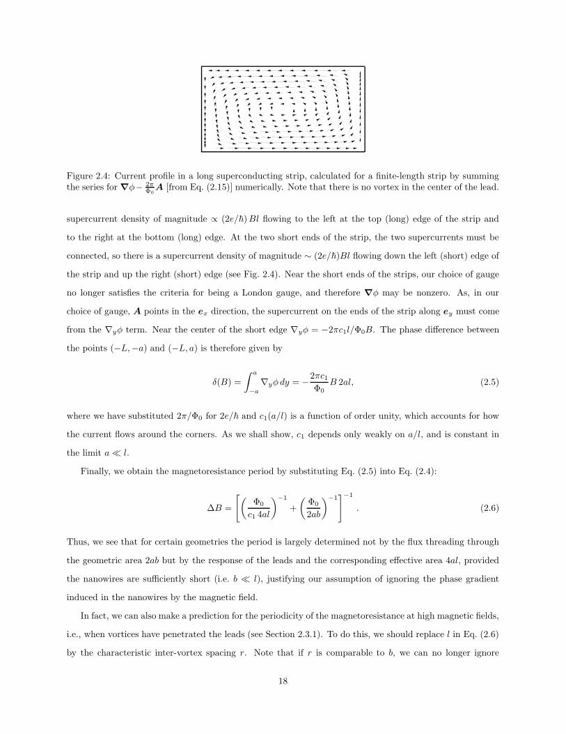
Figure 2.4: Current profile in a long superconducting strip, calculated for a finite-length strip by summingthe series for ∇φ− 2π

Φ0A [from Eq. (2.15)] numerically. Note that there is no vortex in the center of the lead.

supercurrent density of magnitude ∝ (2e/~)Bl flowing to the left at the top (long) edge of the strip and

to the right at the bottom (long) edge. At the two short ends of the strip, the two supercurrents must be

connected, so there is a supercurrent density of magnitude ∼ (2e/~)Bl flowing down the left (short) edge of

the strip and up the right (short) edge (see Fig. 2.4). Near the short ends of the strips, our choice of gauge

no longer satisfies the criteria for being a London gauge, and therefore ∇φ may be nonzero. As, in our

choice of gauge, A points in the ex direction, the supercurrent on the ends of the strip along ey must come

from the ∇yφ term. Near the center of the short edge ∇yφ = −2πc1l/Φ0B. The phase difference between

the points (−L,−a) and (−L, a) is therefore given by

δ(B) =

∫ a

−a

∇yφ dy = −2πc1Φ0

B 2al, (2.5)

where we have substituted 2π/Φ0 for 2e/~ and c1(a/l) is a function of order unity, which accounts for how

the current flows around the corners. As we shall show, c1 depends only weakly on a/l, and is constant in

the limit a l.

Finally, we obtain the magnetoresistance period by substituting Eq. (2.5) into Eq. (2.4):

∆B =

[(Φ0

c1 4al

)−1

+

(Φ0

2ab

)−1]−1

. (2.6)

Thus, we see that for certain geometries the period is largely determined not by the flux threading through

the geometric area 2ab but by the response of the leads and the corresponding effective area 4al, provided

the nanowires are sufficiently short (i.e. b l), justifying our assumption of ignoring the phase gradient

induced in the nanowires by the magnetic field.

In fact, we can also make a prediction for the periodicity of the magnetoresistance at high magnetic fields,

i.e., when vortices have penetrated the leads (see Section 2.3.1). To do this, we should replace l in Eq. (2.6)

by the characteristic inter-vortex spacing r. Note that if r is comparable to b, we can no longer ignore

18

the flux through the AB contour. Furthermore, if r b then the flux through the AB contour determines

periodicity and one recovers the usual Aharonov-Bohm type of phenomenology.

2.3 Mesoscale superconducting leads

In this section and the following one we shall develop a detailed model of the leads and nanowires that

constitute the mesoscopic device.

2.3.1 Vortex-free and vorticial regimes

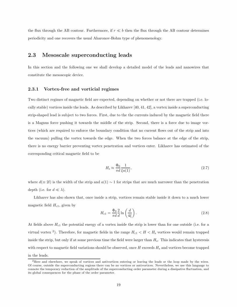
Two distinct regimes of magnetic field are expected, depending on whether or not there are trapped (i.e. lo-

cally stable) vortices inside the leads. As described by Likharev [40, 41, 42], a vortex inside a superconducting

strip-shaped lead is subject to two forces. First, due to the the currents induced by the magnetic field there

is a Magnus force pushing it towards the middle of the strip. Second, there is a force due to image vor-

tices (which are required to enforce the boundary condition that no current flows out of the strip and into

the vacuum) pulling the vortex towards the edge. When the two forces balance at the edge of the strip,

there is no energy barrier preventing vortex penetration and vortices enter. Likharev has estimated of the

corresponding critical magnetic field to be

Hs ≈Φ0

πd

1

ξa(1), (2.7)

where d(≡ 2l) is the width of the strip and a(1) ∼ 1 for strips that are much narrower than the penetration

depth (i.e. for d λ).

Likharev has also shown that, once inside a strip, vortices remain stable inside it down to a much lower

magnetic field Hc1, given by

Hc1 =Φ0

πd

2

dln

(d

4ξ

). (2.8)

At fields above Hc1 the potential energy of a vortex inside the strip is lower than for one outside (i.e. for a

virtual vortex 2). Therefore, for magnetic fields in the range Hc1 < H < Hs vortices would remain trapped

inside the strip, but only if at some previous time the field were larger than Hs. This indicates that hysteresis

with respect to magnetic field variations should be observed, once H exceeds Hs and vortices become trapped

in the leads.

2Here and elsewhere, we speak of vortices and antivortices entering or leaving the leads or the loop made by the wires.Of course, outside the superconducting regions there can be no vortices or antivortices. Nevertheless, we use this language toconnote the temporary reduction of the amplitude of the superconducting order parameter during a dissipative fluctuation, andits global consequences for the phase of the order parameter.

19

In real samples, in addition to the effects analyzed by Likharev, there are also likely to be locations

(e.g. structural defects) that can pin vortices, even for fields smaller than Hc1, so the reproducibility of the

resistance vs. field curve is not generally expected once Hs has been surpassed.

As magnetic field at which vortices first enter the leads is sensitive to the properties of their edges,

we expect only rough agreement with Likharev’s theory. For sample 219-4, using Likharev’s formula, we

estimate Hs = 11 mT (with ξ = 5 nm). The change in regime from fast to slow oscillations is found to

occur at 3.1 mT for that sample [38]. It is possible to determine the critical magnetic fields Hs and Hc1

by the direct imaging of vortices. Although we do not know of such a direct measurement of Hs, Hc1 was

determined by field cooling niobium strips, and found to agree in magnitude to Likharev’s estimate [43].

2.3.2 Phase variation along the edge of the lead

In the previous section it was shown that the periodicity of the magnetoresistance is due to the phase

accumulations associated with the currents along the edges of the leads between the nanowires. Thus, we

should make a precise calculation of the dependence of these currents on the magnetic field, and this we now

do.

Ginzburg-Landau theory

To compute δ(B), we start with the Ginzburg-Landau equation for a thin film as our description of the

mesoscopic superconducting leads:

αψ + β|ψ|2ψ +1

2m∗

(~

i∇− e∗

cA

)2

ψ = 0. (2.9)

Here, ψ is the Ginzburg-Landau order parameter, e∗ (= 2e) is the charge of a Cooper pair and m∗ is its mass,

and α and β may be expressed in terms of the coherence length ξ and critical field Hc via α = −~2/2m∗ξ2

and β = 4πα2/H2c .

The assumptions that the magnetic field is sufficiently weak and that the lead is a narrow strip (compared

with the magnetic penetration depth) allow us to take the amplitude of the order parameter in the leads

to have the value appropriate to an infinite thin film in the absence of the field. By expressing the order

parameter in terms of the (constant) amplitude ψ0 and the (position-dependent) phase φ(r), i.e.,

ψ(r) = ψ0 eiφ(r), (2.10)

20

the Ginzburg-Landau formula for the current density,

J =e∗~

2m∗i

(ψ∗∇ψ − ψ∇ψ∗

)− e∗2

m∗cψ∗ψA(r), (2.11)

becomes

J =e∗

m∗ψ2

0

(~∇φ(r)− e∗

cA(r)

), (2.12)

and [after dividing by eiφ(r)] the real and imaginary parts of the Ginzburg-Landau equation become

0 =

[αψ0 + β ψ3

0 +1

2m∗ψ0

∣∣∣∣~∇φ(r)− e∗

cA(r)

∣∣∣∣2], (2.13a)

0 =~

2

2m∗iψ0

(∇2φ(r)− e∗

~c∇ ·A(r)

). (2.13b)

As long as any spatial inhomogeneity in the gauge-covariant derivative of the phase is weak on the length-

scale of the coherence length[

i.e. ξ∣∣∇φ(r)− e∗

~cA(r)∣∣ 1

], the third term in Eq. (2.13a) is much smaller

than the first two and may be ignored, fixing the amplitude of the order parameter at its field-free infinite thin

film value, viz., ψ0 ≡√−α/β. To compute φ(r) we need to solve the imaginary part of the Ginzburg-Landau

equation.

Formulation as a Laplace problem

We continue to work in the approximation that the amplitude of the order parameter is fixed at ψ0. Starting

from Eq. (2.13b), we see that for our choice of gauge, A = Byex, the phase of the order parameter satisfies

the Laplace equation, ∇2φ = 0. We also enforce the boundary condition that no current flows out of the

superconductor on boundary surface Σ, whose normal is n:

n · j∣∣Σ

= 0, (2.14a)

j ∝(∇φ− 2π

Φ0A). (2.14b)

Solving the Laplace problem for the strip geometry

To solidify the intuition gained via the physical arguments given in Section 2.2, we now determine the phase

profile for an isolated superconducting strip in a magnetic field. This will allow us to determine the constant

c1 in Eq. (2.6), and hence obtain a precise formula for the magnetoresistance period. To this end, we solve

Laplace’s equation for φ subject to the boundary conditions (2.14). We specialize to the case of a rectangular

21

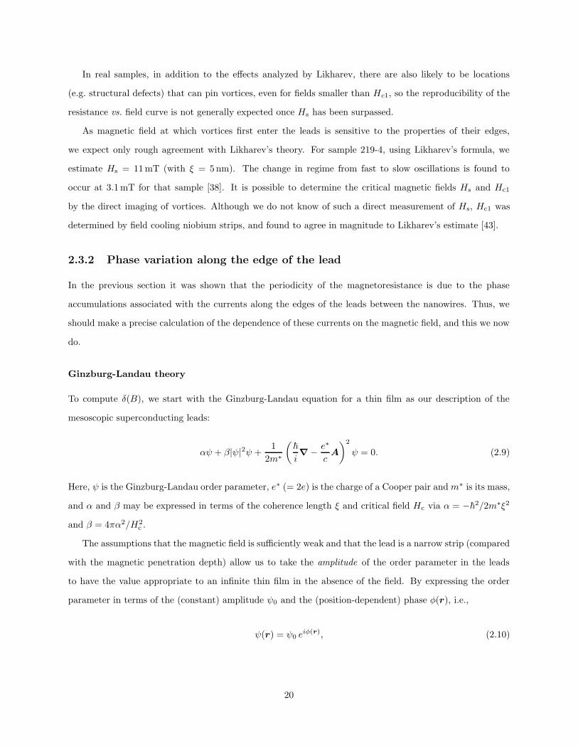
Figure 2.5: Phase profile in the leads in the vicinity of the trench, generated by numerically summing theseries for φ for a finite-length strip. Arrows indicate phases connected by nanowires.

strip 3.

In terms of the coordinates defined in Fig. 2.2, we expand φ(x, y) as the superposition

φ(x, y) = ΘL/R +∑

k

(Ak e

−kx +Bk ekx)

sin(ky), (2.15)

which automatically satisfies Laplace’s equation, although the boundary conditions remain to be satisfied.

ΘL(R) is the phase at the the point in the left (right) lead located half-way between the wires. In other

words ΘL = φ(−L− b, 0) and ΘR = φ(−L, 0) in the coordinate system indicated in Fig. 2.2. ΘL/R are not

determined by the Laplace equation and boundary conditions, but will be determined later by the state of

the nanowires.

We continue working in the gauge A = By ex. The boundary conditions across the edges at y = ±l

(i.e. the long edges) are ∂yφ(x, y = ±l) = 0. These conditions are satisfied by enforcing kn = π(n + 12 )/l,

where n = 0, 1, 2, . . .. The boundary conditions across the edges at x = ±L (i.e. the short edges) are

∂xφ(x = ±L, y) = hy (where h ≡ 2πB/Φ0). This leads to the coefficients in Eq. (2.15) taking the values

Bk = −Ak =h

k3nl

(−1)n

cosh(knL)(n = 0, 1, . . .), (2.16)

and hence to the solution

φ(x, y) =

∞∑

n=0

(−1)n 2h

k3nl cosh(knL)

sin(kny) sinh(knx). (2.17)

Figure 2.5 shows the phase profiles in the leads, in the region close to the trench that separates the leads.

3This specialization is not necessary, but it is convenient and adequately illustrative

22

2.3.3 Period of magnetoresistance for leads having a rectangular strip

geometry

Using the result for the phase that we have just established, we see that the phase profile on the short edge

of the strip at x = −L is given by

φ(−L, y) = −2hl2

π2

∞∑

n=0

(−1)n

(n+ 12 )3

sinπ(n+ 1

2

)y

l, (2.18)

where we have taken the limit L→∞. We would like to evaluate this sum at the points (x, y) = (−L,±a).

This can be done numerically. For nanowires that are close to each other (i.e. for a l), an approximate

value can be found analytically by expanding in a power series in a around y = 0:

φ(−L, a) = φ(−L, 0) + a∂

∂yφ(−L, y)

∣∣∣∣y=0

+a2

2

∂2

∂y2φ(−L, y)

∣∣∣∣y=0

+O(a3).

(2.19)

The first and third terms are evidently zero, as φ is an odd function of y. The second term can be evaluated

by changing the order of summation and differentiation. (Higher-order terms are harder to evaluate, as the

changing of the order of summation and differentiation does not work for them.) Thus, to leading order in

a we have

φ(−L, a) ≈ −8G

π2hla, (2.20)

where G ≡∑∞n=0(−1)n

(2n+1)2 ≈ 0.916 is the Catalan number (see Ref. [44]). This linear approximation is plotted,

together with the actual phase profile obtained by the numerical evaluation of Eq. (2.18), in Fig. 2.6. Hence,

the value of c1 in Eq. (2.5) becomes c1 = 8G/π2 ≈ 0.74, and Eq. (2.6) becomes

B =Φ0

2πh =

π2

8G

Φ0

4al. (2.21)

To obtain this result we used the relation δ(B)/2 = φ(−L, a).

2.3.4 Bridge-lead coupling

In order to simplify our analysis we have assumed that the nanowires do not exert any influence on the order

parameter in the leads. We examine the justification for this assumption in the setting of the experiment

23

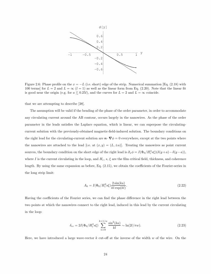
-1 -0.5 0.5 1y

-0.6

-0.4

-0.2

0.2

0.4

0.6

Φ@yD

Figure 2.6: Phase profile on the x = −L (i.e. short) edge of the strip. Numerical summation [Eq. (2.18) with100 terms] for L = 2 and L =∞ (l = 1) as well as the linear form from Eq. (2.20). Note that the linear fitis good near the origin (e.g. for a . 0.25l), and the curves for L = 2 and L =∞ coincide.

that we are attempting to describe [38].

The assumption will be valid if the bending of the phase of the order parameter, in order to accommodate

any circulating current around the AB contour, occurs largely in the nanowires. As the phase of the order

parameter in the leads satisfies the Laplace equation, which is linear, we can superpose the circulating-

current solution with the previously-obtained magnetic-field-induced solution. The boundary conditions on

the right lead for the circulating-current solution are n ·∇φ = 0 everywhere, except at the two points where

the nanowires are attached to the lead [i.e. at (x, y) = (L,±a)]. Treating the nanowires as point current

sources, the boundary condition on the short edge of the right lead is ∂xφ = I(Φ0/H2c sξ)(δ(y+a)−δ(y−a)),

where I is the current circulating in the loop, and Hc, s, ξ are the film critical field, thickness, and coherence

length. By using the same expansion as before, Eq. (2.15), we obtain the coefficients of the Fourier-series in

the long strip limit:

Ak = I(Φ0/H2c sξ)

2 sin(ka)

kl exp(kl). (2.22)

Having the coefficients of the Fourier series, we can find the phase difference in the right lead between the

two points at which the nanowires connect to the right lead, induced in this lead by the current circulating

in the loop:

δcc = 2I(Φ0/H2c sξ)

k=1/w∑

n=0

sin2(ka)

kl∼ ln(2l/πw). (2.23)

Here, we have introduced a large wave-vector k cut-off at the inverse of the width w of the wire. On the

24

other hand, the current flowing through the wire is

ξH2c

Φ0ws

∆θ

b, (2.24)

where ξ, Hc, and s are the wire coherence length, critical field, and height (recall that b is the wire length).

To support a circulating current that corresponds to a phase accumulation of ∆θ along one of the wires, the

phase difference between the two nanowires in the lead must be on the order of

δcc = ∆θw

b

(H2

c sξ)wire

(H2c sξ)film

ln

(2l

πw

). (2.25)

For our experiments [38], we estimate that the ratio of δcc to ∆θ is always less than 20%, validating the

assumption of weak coupling.

2.3.5 Strong nanowires

We remark that the assumption of weak nanowires is not obligatory for the computation the magnetore-

sistance period . Dropping this assumption would leave the period of the magnetoresistance oscillations

unchanged.

To see this, consider φ11, i.e., the phase profile in the leads that corresponds to the lowest energy solution

of the Ginzburg-Landau equation at field corresponding to the first resistance minimum [i.e. at B being

the first non-zero solution of Eq. (2.4)]. For this case, and for short wires, the phase gain along the wires

is negligible, whereas the phase gain in the leads is 2π, even for wires with large critical current. Excited

states, with vortices threading the AB contour, can be constructed by the linear superposition of φ11 with

φ0nv, where φ0nv

is the phase profile with nv vortices at no applied magnetic field.

This construction requires that the nanowires are narrow, but works independently of whether nanowires

are strong or weak, in the limit that H Hc. The energy of the lowest energy state always reaches

its minimum when the applied magnetic field is such that there is no phase gain (i.e. no current) in the

nanowires. By the above construction, it is clear that the resistance of the device at this field is the same as

at zero field, and therefore the minimum possible.

Therefore, our calculation of the period is valid, independent of whether the nanowires are weak or

strong. However, the assumption of weak nanowires is necessary for the computation of magnetoresistance

amplitude, which we present in the following section.

25

2.4 Parallel superconducting nanowires and intrinsic resistance

In this section we consider the intrinsic resistance of the device. We assume that this resistance is due to

thermally activated phase slips (TAPS) of the order parameter, and that these occur within the nanowires.

Equivalently, these processes may be thought of as thermally activated vortex flow across the nanowires.

Specifically, we shall derive analytical results for the asymptotic cases of nanowires that are either short or

long, compared to coherence length, i.e. Josephson junctions [3, 4, 5] or Langer-Ambegaokar-McCumber-

Halperin (LAMH) wires [6, 7]; see also Ref. [29]. We have not been able to find a closed-form expression for

the intrinsic resistance in the intermediate-length regime, so we shall consider that case numerically.

There are two (limiting) kinds of experiments that may be performed: fixed total current and fixed

voltage. In the first kind, a specified current is driven through the device and the time-averaged voltage

is measured. Here, this voltage is proportional to the net number of phase slips (in the forward direction)

per unit time, which depends on the height of the free-energy barriers for phase slips. Why do we expect

minima in the resistance at magnetic fields corresponding to 2δ = 2mπ and maxima at 2δ = (2m+ 1)π for

m integral, at least at vanishingly small total current through both wires? For 2δ = 2mπ the nanowires

are unfrustrated, in the sense that there is no current through either wire in the lowest local minimum of

the free energy. On the other hand, for 2δ = (2m+ 1)π the nanowires are maximally frustrated: there is a

nonzero circulating current around the AB contour. Quite generally, the heights of the free-energy barriers

protecting locally stable states decrease with increasing current through a wire, and thus the frustrated

situation is more susceptible to dissipative fluctuations, and hence shows higher resistance. Note, however,

that due to the inter-bridge coupling caused by the phase constraint, the resistance of the full device is more

subtle than the mere addition of the resistances of two independent, parallel nanowires, both carrying the

requisite circulating current.

In the second kind of experiment, a fixed voltage is applied across the device and the total current is

measured. In this situation, the inter-lead voltage is fixed, and therefore the phase drop along each wire is

a fixed function of time. Hence, there is no inter-bridge coupling in the fixed voltage regime. Therefore,

the resistance of the device would not exhibit magnetic field dependence. If the voltage is fixed far away

from the wires, but not in the immediate vicinity of the wires, so that the phase drop along each wire is

not rigidly fixed, then some of the magnetic field dependence of the resistance would be restored. In our

experiments on two-wire devices, we believe that the situation lies closer to the fixed current limit than to

the fixed voltage limit, and therefore we shall restrict our attention to the former limit.

In the fixed-current regime, the relevant independent thermodynamic variable for the device is the total

current through the pair of wires, i.e., I ≡ I1 +I2. Therefore, the appropriate free energy to use, in obtaining

26

the barrier heights for phase slips, is the Gibbs free energy G(I), as discussed by McCumber [30], rather

than the Helmholtz free energy F (Θ) 4. In the Helmholtz free energy the independent variable can be taken

to be Θ ≡ ΘL −ΘR, i.e., the phase difference across the center of the “trench,” defined modulo 2π. G(I) is

obtained from F (Θ) via the appropriate Legendre transformation:

G(I) = F (Θ)− ~

2eIΘ, (2.26)

where the second term represents the work done on the system by the external current source. F (Θ) is the

sum of the Helmholtz free energies for the individual nanowires:

F (Θ) = F1(θ1) + F2(θ2), (2.27)

where F1(2)(θ1(2)) is the Ginzburg-Landau free energy for first (second) wire and a simplified notation has

been used θ1 ≡ θ1,L←R and θ2 ≡ θ2,L←R. θ1 and θ2 are related to each other and to Θ through the phase

constraint Eq. (2.2).

2.4.1 Short nanowires: Josephson junction limit

If the nanowires are sufficiently short, they may be treated as Josephson junctions. Unlike the case of long

nanowires, described in the following subsection, in this Josephson regime there is no metastability, i.e., the

free energy of each junction is a single-valued function of the phase difference, modulo 2π, across it. The

phase constraint then implies that there is a rigid difference between the phases across the two junctions.

As a consequence, nv can be set to zero. The Gibbs free energy in such a configuration is then

G(I) = − ~

2e

(Ic1 cos(θ1) + Ic2 cos(θ2) + IΘ

), (2.28)

where Ic1 and Ic2 are the critical currents for the junctions. In thermodynamic equilibrium, the Gibbs free

energy must be minimized, so the dependent variable Θ must be chosen such that ∂G(I)/∂Θ = 0.

Using θ1 = Θ + δ and θ2 = Θ− δ, G(I) may be rewritten in the form

G(I) = − ~

2e

(√(Ic1 + Ic2)2 cos2 δ + (Ic1 − Ic2)2 sin2 δ · cos(ϑ) + I ϑ1

), (2.29)

where we have shifted the free energy by an additive constant(

~

2e

)I tan−1

[(Ic1−Ic2Ic2+Ic1

)tan δ

], and ϑ ≡

4Recall that the Helmholtz free energy is obtained by minimizing the Ginzburg-Landau free energy functional with respect

to the order parameter function ψ(r), subject to the phase accumulation constraintR

R

Ldr · ∇φ = θ.

27

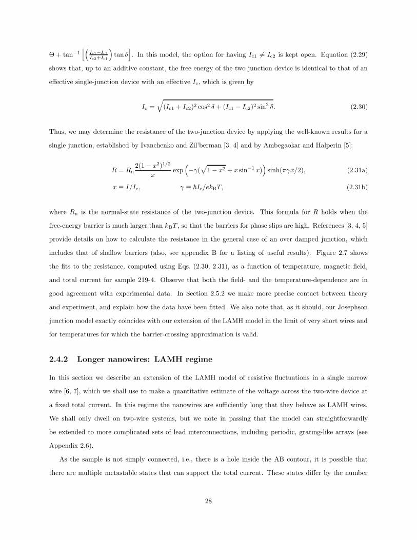
Θ + tan−1[(

Ic1−Ic2Ic2+Ic1

)tan δ

]. In this model, the option for having Ic1 6= Ic2 is kept open. Equation (2.29)

shows that, up to an additive constant, the free energy of the two-junction device is identical to that of an

effective single-junction device with an effective Ic, which is given by

Ic =

√(Ic1 + Ic2)2 cos2 δ + (Ic1 − Ic2)2 sin2 δ. (2.30)

Thus, we may determine the resistance of the two-junction device by applying the well-known results for a

single junction, established by Ivanchenko and Zil’berman [3, 4] and by Ambegaokar and Halperin [5]:

R = Rn2(1− x2)1/2

xexp

(−γ(

√1− x2 + x sin−1 x)

)sinh(πγx/2), (2.31a)

x ≡ I/Ic, γ ≡ ~Ic/ekBT, (2.31b)

where Rn is the normal-state resistance of the two-junction device. This formula for R holds when the

free-energy barrier is much larger than kBT , so that the barriers for phase slips are high. References [3, 4, 5]

provide details on how to calculate the resistance in the general case of an over damped junction, which

includes that of shallow barriers (also, see appendix B for a listing of useful results). Figure 2.7 shows

the fits to the resistance, computed using Eqs. (2.30, 2.31), as a function of temperature, magnetic field,

and total current for sample 219-4. Observe that both the field- and the temperature-dependence are in

good agreement with experimental data. In Section 2.5.2 we make more precise contact between theory

and experiment, and explain how the data have been fitted. We also note that, as it should, our Josephson

junction model exactly coincides with our extension of the LAMH model in the limit of very short wires and

for temperatures for which the barrier-crossing approximation is valid.

2.4.2 Longer nanowires: LAMH regime

In this section we describe an extension of the LAMH model of resistive fluctuations in a single narrow

wire [6, 7], which we shall use to make a quantitative estimate of the voltage across the two-wire device at

a fixed total current. In this regime the nanowires are sufficiently long that they behave as LAMH wires.

We shall only dwell on two-wire systems, but we note in passing that the model can straightforwardly

be extended to more complicated sets of lead interconnections, including periodic, grating-like arrays (see

Appendix 2.6).

As the sample is not simply connected, i.e., there is a hole inside the AB contour, it is possible that

there are multiple metastable states that can support the total current. These states differ by the number

28

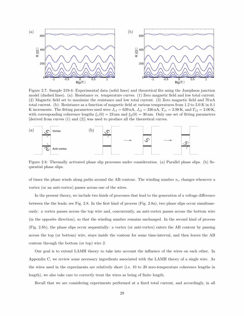
(a)

-1 -0.5 0 0.5 1B(µΤ)

0

200

400

600R

(Ω

)(b)

-1 -0.5 0 0.5 1B(µΤ)

0

200

400

600

R (

Ω)

Figure 2.7: Sample 219-4: Experimental data (solid lines) and theoretical fits using the Josephson junctionmodel (dashed lines). (a): Resistance vs. temperature curves. (1) Zero magnetic field and low total current.(2) Magnetic field set to maximize the resistance and low total current. (3) Zero magnetic field and 70 nAtotal current. (b): Resistance as a function of magnetic field at various temperatures from 1.2 to 2.0 K in 0.1K increments. The fitting parameters used were Jc1 = 639 nA, Jc2 = 330 nA, Tc1 = 2.98 K, and Tc2 = 2.00 K,with corresponding coherence lengths ξ1(0) = 23 nm and ξ2(0) = 30 nm. Only one set of fitting parameters[derived from curves (1) and (2)] was used to produce all the theoretical curves.

Anti-vortex

Vortex(a) (b)

Figure 2.8: Thermally activated phase slip processes under consideration. (a) Parallel phase slips. (b) Se-quential phase slips.

of times the phase winds along paths around the AB contour. The winding number nv changes whenever a

vortex (or an anti-vortex) passes across one of the wires.

In the present theory, we include two kinds of processes that lead to the generation of a voltage difference

between the the leads; see Fig. 2.8. In the first kind of process (Fig. 2.8a), two phase slips occur simultane-

ously: a vortex passes across the top wire and, concurrently, an anti-vortex passes across the bottom wire

(in the opposite direction), so that the winding number remains unchanged. In the second kind of process

(Fig. 2.8b), the phase slips occur sequentially: a vortex (or anti-vortex) enters the AB contour by passing

across the top (or bottom) wire, stays inside the contour for some time-interval, and then leaves the AB

contour through the bottom (or top) wire 2.

Our goal is to extend LAMH theory to take into account the influence of the wires on each other. In

Appendix C, we review some necessary ingredients associated with the LAMH theory of a single wire. As

the wires used in the experiments are relatively short (i.e. 10 to 20 zero-temperature coherence lengths in

length), we also take care to correctly treat the wires as being of finite length.

Recall that we are considering experiments performed at a fixed total current, and accordingly, in all

29

configurations of the order parameter this current must be shared between the top and bottom wires. We

shall refer to this sharing,

I = I1 + I2, (2.32)

as the total current constraint . Let us begin by considering a phase-slip event in a device with an isolated

wire. While the order parameter in that wire pinches down, the end-to-end phase accumulation must adjust

to maintain the prescribed value of the current through the wire. Now consider the two-wire device, and

consider a phase slip event in one of the wires. As in the single-wire case, the phase accumulation will adjust,

but in so doing it will alter the current flowing through other wire. Thus, in the saddle-point configuration

of the two-wire system the current splitting will differ from that in the locally stable initial (and final) state.

Taking into account the two kinds of phase-slip processes, and imposing the appropriate constraints

(i.e. the total current constraint and the phase constraint), we construct the possible metastable and saddle-

point configurations of the order parameter in the two-wire system. Finally, we compute the relevant rates

of thermally activated transitions between these metastable states, construct a Markov chain [45], and

determine the steady-state populations of these states. Thus, we are able to evaluate the time-average of

the voltage generated between the leads at fixed current due to these various dissipative fluctuations. We

mention that we have not allowed for wires of distinct length or constitution (so that the Ginzburg-Landau

parameters describing them are taken to be identical). This is done solely to simplify the analysis; extensions

to more general cases would be straightforward but tedious.

Parallel pair of nanowires

The total Gibbs free energy for the two-wire system is given by

G(I) = F1(θ1) + F2(θ2)− 4EΘ · (J1 + J2). (2.33)

Here, we have followed MH by rewriting the current-phase term in terms of dimensionless currents in wires

i = 1, 2, i.e., Ji defined via Ii = 8πcJiE/Φ0. Moreover, E ≡ H2c ξσ8π is the condensate energy density per

unit length of wire, and Fi(θi) is the Helmholtz free energy for a single wire along which there is a total

phase accumulation of θi. The precise form of Fi(θi) depends on whether the wire is in a metastable or

saddle-point state.

We are concerned with making stationary the total Gibbs free energy at specified total current I , subject

to the phase constraint, Eq. (2.2). This can be accomplished by making stationary the Helmholtz free energy

on each wire, subject to both the total current constraint and the phase constraint, but allowing θ1 and θ2

30

to vary so as to satisfy these constraints—in effect, adopting the total current I as the independent variable.

The stationary points of the Helmholtz free energy for a single wire are reviewed in Appendix C as implicit

functions of θi, i.e., the end-to-end phase accumulation along the wire. The explicit variable used there is

Ji, which is related to θi via Eq. (C.21).

Analytical treatment in the limit of long nanowires

In the long-wire limit, we can compute the resistance analytically by making use of the single-wire free energy

and end-to-end phase accumulation derived by Langer and Ambegaokar [6] (and extended by McCumber [30]

for the case of the constant-current ensemble). Throughout the present subsection we shall be making an

expansion in powers of 1/b, where b is the length of the wire measured in units of the coherence length,

keeping terms only to first order in 1/b. Thus, one arrives at formulæ for the end-to-end phase accumulations

and Helmholtz free energies for single-wire metastable (m) and saddle-point (sp) states [30]:

θm(κ) = κb, (2.34a)

θsp(κ) = κb+ 2 tan−1

(1− 3κ2

2κ2

)1/2

, (2.34b)

Fm(κ) = −E(b(1− κ2)2

), (2.34c)

Fsp(κ) = −E(b(1− κ2)2 − 8

√2

3

√1− 3κ2

), (2.34d)

where κ is defined via Ji = κi(1 − κ2i ). In the small-current limit, one can make the further simplification

that Ji ≈ κi; henceforth we shall keep terms only up to first order in κ. To this order, the phase difference

along a wire in a saddle-point state becomes

θsp = κb+ π − 2√

2κ. (2.35)

Next, we make use of these single-wire LAMH results to find the metastable and saddle-point states

of the two-wire system, and use them to compute the corresponding barrier heights and, hence, transition

rates. At low temperatures, it is reasonable to expect that only the lowest few metastable states will be

appreciably occupied. These metastable states, as well as the saddle-point states between them, correspond

31

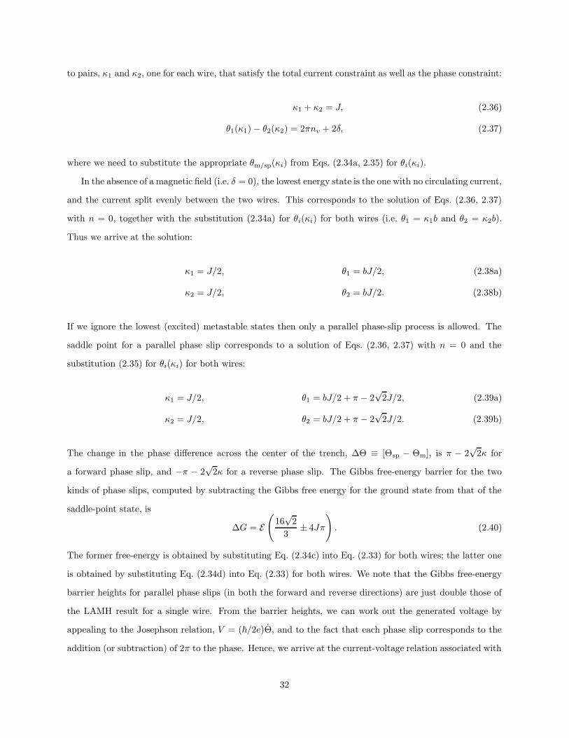
to pairs, κ1 and κ2, one for each wire, that satisfy the total current constraint as well as the phase constraint:

κ1 + κ2 = J, (2.36)

θ1(κ1)− θ2(κ2) = 2πnv + 2δ, (2.37)

where we need to substitute the appropriate θm/sp(κi) from Eqs. (2.34a, 2.35) for θi(κi).

In the absence of a magnetic field (i.e. δ = 0), the lowest energy state is the one with no circulating current,

and the current split evenly between the two wires. This corresponds to the solution of Eqs. (2.36, 2.37)

with n = 0, together with the substitution (2.34a) for θi(κi) for both wires (i.e. θ1 = κ1b and θ2 = κ2b).

Thus we arrive at the solution:

κ1 = J/2, θ1 = bJ/2, (2.38a)

κ2 = J/2, θ2 = bJ/2. (2.38b)

If we ignore the lowest (excited) metastable states then only a parallel phase-slip process is allowed. The

saddle point for a parallel phase slip corresponds to a solution of Eqs. (2.36, 2.37) with n = 0 and the

substitution (2.35) for θi(κi) for both wires:

κ1 = J/2, θ1 = bJ/2 + π − 2√

2J/2, (2.39a)

κ2 = J/2, θ2 = bJ/2 + π − 2√

2J/2. (2.39b)

The change in the phase difference across the center of the trench, ∆Θ ≡ [Θsp − Θm], is π − 2√

2κ for

a forward phase slip, and −π − 2√

2κ for a reverse phase slip. The Gibbs free-energy barrier for the two

kinds of phase slips, computed by subtracting the Gibbs free energy for the ground state from that of the

saddle-point state, is

∆G = E(

16√

2

3± 4Jπ

). (2.40)

The former free-energy is obtained by substituting Eq. (2.34c) into Eq. (2.33) for both wires; the latter one

is obtained by substituting Eq. (2.34d) into Eq. (2.33) for both wires. We note that the Gibbs free-energy

barrier heights for parallel phase slips (in both the forward and reverse directions) are just double those of

the LAMH result for a single wire. From the barrier heights, we can work out the generated voltage by

appealing to the Josephson relation, V = (~/2e)Θ, and to the fact that each phase slip corresponds to the

addition (or subtraction) of 2π to the phase. Hence, we arrive at the current-voltage relation associated with

32

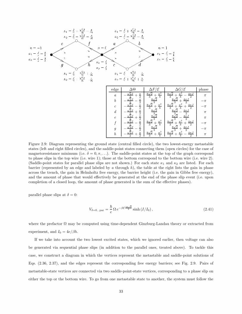
edge ∆Θ ∆F/E ∆G/E phase

a −√

2J2 + π

28√

23 + π2

b8√

23 + π2

b − 4πJ2 π

b −√

2J2 − π

28√

23

8√

23 + 4πJ

2 −πc −

√2J2 − π

28√

23 + π2

b8√

23 + π2

b + 4πJ2 −π

d −√

2J2 + π

28√

23

8√

23 − 4πJ

2 π

e −√

2J2 + π

28√

23

8√

23 − 4πJ

2 π

f −√

2J2 − π

28√

23 + π2

b8√

23 + π2

b + 4πJ2 −π

g −√

2J2 − π

28√

23

8√

23 + 4πJ

2 −πh −

√2J2 + π

28√

23 + π2

b8√

23 + π2

b − 4πJ2 π

Figure 2.9: Diagram representing the ground state (central filled circle), the two lowest-energy metastablestates (left and right filled circles), and the saddle-point states connecting them (open circles) for the case ofmagnetoresistance minimum (i.e. δ = 0, π, . . .). The saddle-point states at the top of the graph correspondto phase slips in the top wire (i.e. wire 1); those at the bottom correspond to the bottom wire (i.e. wire 2).(Saddle-point states for parallel phase slips are not shown.) For each state κ1 and κ2 are listed. For eachbarrier (represented by an edge and labeled by a through h), the table at the right lists the gain in phaseacross the trench, the gain in Helmholtz free energy, the barrier height (i.e. the gain in Gibbs free energy),and the amount of phase that would effectively be generated at the end of the phase slip event (i.e. uponcompletion of a closed loop, the amount of phase generated is the sum of the effective phases).

parallel phase slips at δ = 0:

Vδ=0 , par =~

eΩ e−βE 16

√2

3 sinh (I/I0) , (2.41)

where the prefactor Ω may be computed using time-dependent Ginzburg-Landau theory or extracted from

experiment, and I0 = 4e/βh.

If we take into account the two lowest excited states, which we ignored earlier, then voltage can also

be generated via sequential phase slips (in addition to the parallel ones, treated above). To tackle this

case, we construct a diagram in which the vertices represent the metastable and saddle-point solutions of

Eqs. (2.36, 2.37), and the edges represent the corresponding free energy barriers; see Fig. 2.9. Pairs of

metastable-state vertices are connected via two saddle-point-state vertices, corresponding to a phase slip on

either the top or the bottom wire. To go from one metastable state to another, the system must follow the

33

edge out of the starting metastable state leading to the desired saddle-point state. We assume that, once

the saddle-point state is reached, the top of the barrier has been passed and the order parameter relaxes

to the target metastable state. (To make the graph more legible, we have omitted drawing the edge that

corresponds to this relaxation process.) To find the Gibbs free-energy difference between a metastable state

and a saddle-point state, we need to know the phase difference across the center of the trench. To resolve

the ambiguity of 2π in the definition of Θ, the phase difference can be found by following the wire with no

phase slip. To further improve the legibility of Fig. 2.9, the free-energy barriers are listed in a separate table

to the right. Note, that a phase slip on just one of the wires, being only half of the complete process, can

be regarded to a gain in phase of ±π for the purposes of calculating voltage, as indicated in both the graph

and the table.

Once the table of barrier heights has been computed, we can construct a Markov chain on a directed

graph, where the metastable states are the vertices—in effect, an explicit version of our diagram. In general,

each pair of neighboring metastable states, sn and sn+1, are connected by four directed edges:

sn −−−−−→top

sn+1 sn −−−−−→bottom

sn+1 (2.42a)

sn ←−−−−−top

sn+1 sn ←−−−−−bottom

sn+1 (2.42b)

where the probability to pass along a particular edge is given by P (·) = exp−β∆G(·), in which ∆G(·) may

be read off from the table in Fig. 2.9.

We denote the occupation probability of the nth metastable state by on, where n corresponds to the

n in the phase constraint (2.2). on may be computed in the standard way, by diagonalizing the matrix

representing the Markov chain [45]. Each move in the Markov chain can be associated with a gain in phase

across the device of ±π, as specified in Fig. 2.9. Thus, we may compute the rate of phase-gain, and hence

the voltage:

V =Ω~

4e

∑

〈nm〉

on

gn,m

(P (sn −−→

topsm)− P (sn −−→

botsm)

), (2.43)

where the rate prefactor Ω is to be determined, 〈nm〉 indicates that the sum runs over neighboring states

only, and gn,m keeps track of the sign of the phase-gain for reverse phase-slips:

gn,m =

1, if m > n,

−1, if m < n.(2.44)

For the case δ = 0, and keeping the bottom three states only, the voltage generated via sequential phase

34

edge ∆Θ ∆F/E ∆G/E phase

1 −√

2J2 + π

28√

23 − π2

b8√

23 − π2

b − 4πJ2 π

2 −√

2J2 − π

28√

23 − π2

b8√

23 − π2

b + 4πJ2 −π

3 −√

2J2 − π

28√

23 − π2

b8√

23 − π2

b + 4πJ2 −π

4 −√

2J2 + π

28√

23 − π2

b8√

23 − π2

b − 4πJ2 π

Figure 2.10: Diagram and corresponding Table for the case of magnetoresistance maxima (i.e. δ =π/2, 3π/2, . . .). See the caption to Fig. 2.9 for explanation of the diagram.

slips turns out to be

Vδ=0 , seq =2~

eΩ e−βE

“

8√

23

+ π2

b

”

sinh(I/2I0). (2.45)

Having dealt with the case of δ = 0 (and hence obtained the value of the resistance at magnetic fields

corresponding to resistance minima), we now turn to the case of δ = π/2, i.e., resistance maxima.

In this half-flux quantum situation, there are two degenerate lowest-energy states, with opposite circulat-

ing currents. These states are connected by saddle-point states in which a phase-slip is occurring on either

the top or bottom wire. The diagram of the degenerate ground states and the saddle-point states connecting

them is shown in Fig. 2.10. By comparing the diagram with the associated Table, it is easy to see that

the free-energy barriers are biased by the current, making clockwise traversals of Fig. 2.10 more probable

than counter-clockwise traversals. As there are only two metastable states being considered, and as they are

degenerate, it is unnecessary to go through the Markov chain calculation; clearly, the two states each have

a population of 1/2. The voltage being generated by the sequential phase-slip is then given by

Vδ=π/2, seq =~

2eΩ e−βE

“

8√

23−π2

b

”

sinh(I/2I0). (2.46)

Vδ=π/2, seq is larger than the sum of Vδ=0, seq and Vδ=0, par, so, as expected, the resistance is highest at

magnetic fields corresponding to δ = π/2. For very long wires, the perturbation of one wire when a phase

slip occurs in the other is very small, and therefore we expect that the dependence of resistance on magnetic

35

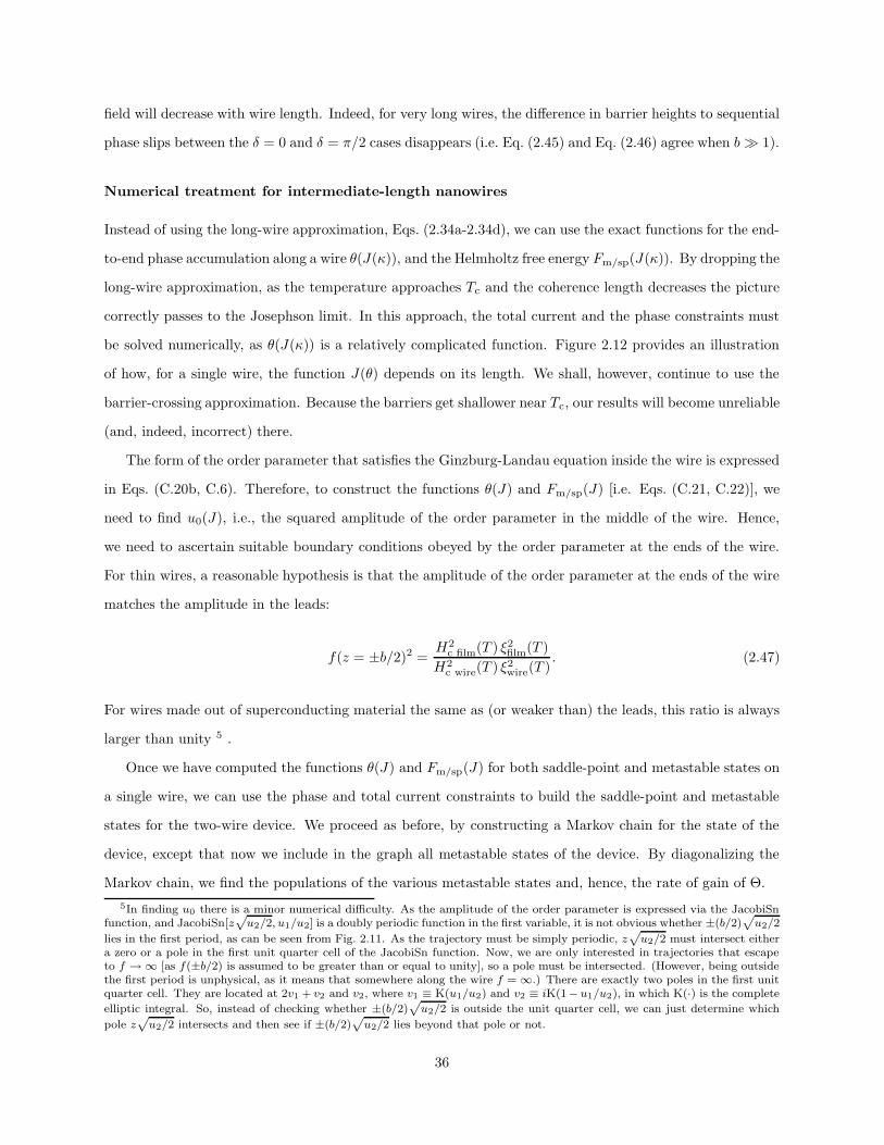
field will decrease with wire length. Indeed, for very long wires, the difference in barrier heights to sequential

phase slips between the δ = 0 and δ = π/2 cases disappears (i.e. Eq. (2.45) and Eq. (2.46) agree when b 1).

Numerical treatment for intermediate-length nanowires

Instead of using the long-wire approximation, Eqs. (2.34a-2.34d), we can use the exact functions for the end-

to-end phase accumulation along a wire θ(J(κ)), and the Helmholtz free energy Fm/sp(J(κ)). By dropping the

long-wire approximation, as the temperature approaches Tc and the coherence length decreases the picture

correctly passes to the Josephson limit. In this approach, the total current and the phase constraints must

be solved numerically, as θ(J(κ)) is a relatively complicated function. Figure 2.12 provides an illustration

of how, for a single wire, the function J(θ) depends on its length. We shall, however, continue to use the

barrier-crossing approximation. Because the barriers get shallower near Tc, our results will become unreliable

(and, indeed, incorrect) there.

The form of the order parameter that satisfies the Ginzburg-Landau equation inside the wire is expressed

in Eqs. (C.20b, C.6). Therefore, to construct the functions θ(J) and Fm/sp(J) [i.e. Eqs. (C.21, C.22)], we

need to find u0(J), i.e., the squared amplitude of the order parameter in the middle of the wire. Hence,

we need to ascertain suitable boundary conditions obeyed by the order parameter at the ends of the wire.

For thin wires, a reasonable hypothesis is that the amplitude of the order parameter at the ends of the wire

matches the amplitude in the leads:

f(z = ±b/2)2 =H2

c film(T ) ξ2film(T )

H2c wire(T ) ξ2wire(T )

. (2.47)

For wires made out of superconducting material the same as (or weaker than) the leads, this ratio is always

larger than unity 5 .

Once we have computed the functions θ(J) and Fm/sp(J) for both saddle-point and metastable states on

a single wire, we can use the phase and total current constraints to build the saddle-point and metastable

states for the two-wire device. We proceed as before, by constructing a Markov chain for the state of the

device, except that now we include in the graph all metastable states of the device. By diagonalizing the

Markov chain, we find the populations of the various metastable states and, hence, the rate of gain of Θ.

5In finding u0 there is a minor numerical difficulty. As the amplitude of the order parameter is expressed via the JacobiSnfunction, and JacobiSn[z

p

u2/2, u1/u2] is a doubly periodic function in the first variable, it is not obvious whether ±(b/2)p

u2/2

lies in the first period, as can be seen from Fig. 2.11. As the trajectory must be simply periodic, zp

u2/2 must intersect eithera zero or a pole in the first unit quarter cell of the JacobiSn function. Now, we are only interested in trajectories that escapeto f → ∞ [as f(±b/2) is assumed to be greater than or equal to unity], so a pole must be intersected. (However, being outsidethe first period is unphysical, as it means that somewhere along the wire f = ∞.) There are exactly two poles in the first unitquarter cell. They are located at 2v1 + v2 and v2, where v1 ≡ K(u1/u2) and v2 ≡ iK(1−u1/u2), in which K(·) is the complete

elliptic integral. So, instead of checking whether ±(b/2)p

u2/2 is outside the unit quarter cell, we can just determine which

pole zp

u2/2 intersects and then see if ±(b/2)p

u2/2 lies beyond that pole or not.

36

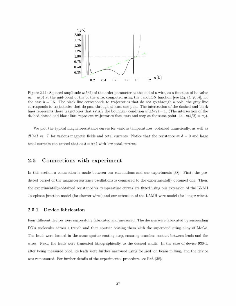
Figure 2.11: Squared amplitude u(b/2) of the order parameter at the end of a wire, as a function of its valueu0 = u(0) at the mid-point of the of the wire, computed using the JacobiSN function [see Eq. (C.20b)], forthe case b = 16. The black line corresponds to trajectories that do not go through a pole; the gray linecorresponds to trajectories that do pass through at least one pole. The intersection of the dashed and blacklines represents those trajectories that satisfy the boundary condition u(±b/2) = 1. (The intersection of thedashed-dotted and black lines represent trajectories that start and stop at the same point, i.e., u(b/2) = u0).

We plot the typical magnetoresistance curves for various temperatures, obtained numerically, as well as

dV/dI vs. T for various magnetic fields and total currents. Notice that the resistance at δ = 0 and large

total currents can exceed that at δ = π/2 with low total-current.

2.5 Connections with experiment

In this section a connection is made between our calculations and our experiments [38]. First, the pre-

dicted period of the magnetoresistance oscillations is compared to the experimentally obtained one. Then,

the experimentally-obtained resistance vs. temperature curves are fitted using our extension of the IZ-AH

Josephson junction model (for shorter wires) and our extension of the LAMH wire model (for longer wires).

2.5.1 Device fabrication

Four different devices were successfully fabricated and measured. The devices were fabricated by suspending

DNA molecules across a trench and then sputter coating them with the superconducting alloy of MoGe.

The leads were formed in the same sputter-coating step, ensuring seamless contact between leads and the

wires. Next, the leads were truncated lithographically to the desired width. In the case of device 930-1,

after being measured once, its leads were further narrowed using focused ion beam milling, and the device

was remeasured. For further details of the experimental procedure see Ref. [38].

37

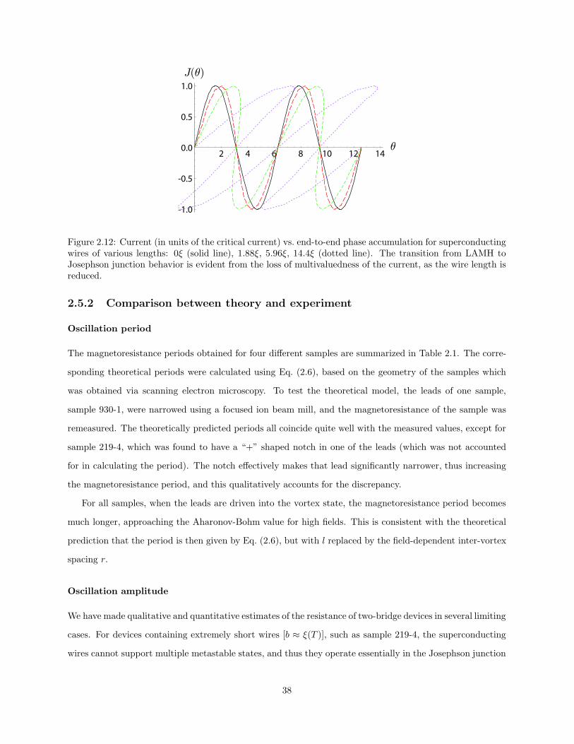
2 4 6 8 10 12 14

-1.0

-0.5

0.5

1.0

0.0 µ

J(µ)

Figure 2.12: Current (in units of the critical current) vs. end-to-end phase accumulation for superconductingwires of various lengths: 0ξ (solid line), 1.88ξ, 5.96ξ, 14.4ξ (dotted line). The transition from LAMH toJosephson junction behavior is evident from the loss of multivaluedness of the current, as the wire length isreduced.

2.5.2 Comparison between theory and experiment

Oscillation period

The magnetoresistance periods obtained for four different samples are summarized in Table 2.1. The corre-

sponding theoretical periods were calculated using Eq. (2.6), based on the geometry of the samples which

was obtained via scanning electron microscopy. To test the theoretical model, the leads of one sample,

sample 930-1, were narrowed using a focused ion beam mill, and the magnetoresistance of the sample was

remeasured. The theoretically predicted periods all coincide quite well with the measured values, except for

sample 219-4, which was found to have a “+” shaped notch in one of the leads (which was not accounted

for in calculating the period). The notch effectively makes that lead significantly narrower, thus increasing

the magnetoresistance period, and this qualitatively accounts for the discrepancy.

For all samples, when the leads are driven into the vortex state, the magnetoresistance period becomes

much longer, approaching the Aharonov-Bohm value for high fields. This is consistent with the theoretical

prediction that the period is then given by Eq. (2.6), but with l replaced by the field-dependent inter-vortex

spacing r.

Oscillation amplitude

We have made qualitative and quantitative estimates of the resistance of two-bridge devices in several limiting

cases. For devices containing extremely short wires [b ≈ ξ(T )], such as sample 219-4, the superconducting

wires cannot support multiple metastable states, and thus they operate essentially in the Josephson junction

38

Sample b (nm) 2a (nm) 2l (nm) Theoretical period (µT) Measured period (µT) error205-4 121 266 11267 929.21 947. 1.9%219-4 137 594 12062 388.73 456.6 12.8%930-1 141 2453 14480 78.41 77.5 −1.2%930-1 (shaved) 141 2453 8930 127.14 128.3 0.9%205-2 134 4046 14521 47.41 48.9 3.0%

Table 2.1: Comparison between measured and theoretical magnetoresistance periods. The geometries of thesamples were obtained via scanning electron microscopy and used to compute the periods theoretically; seethe text for additional details.

Figure 2.13: Sample 219-4: Resistance vs. temperature measurements in zero magnetic field (open circles)and at a magnetic field of 228µT (solid circles) corresponding to a maximum change in magnetoresistance.The lines are theoretical fits, based on the short-wire (Josephson) limit of the LAMH theory, using the fol-lowing fitting parameters: Jc1 = 639 nA, Jc2 = 330 nA, Tc1 = 2.98 K, and Tc2 = 2.00 K (with correspondingcoherence lengths ξ1(0) = 20 nm and ξ2(0) = 26 nm).

limit, but with the junction critical current being a function of temperature given by LAMH theory as

Ic(T ) = Ic(0)(1− T/Tc)3/2. (2.48)

A summary of fits to the data for this sample, using the Josephson junction limit, is shown in Fig. 2.7. On

the other hand, for longer wires it is essential to take into account the multiple metastable states, as is the

case for sample 930-1, which has wires of intermediate length. A summary of numerical fits for this sample

is shown in Fig. 2.14. In all cases, only the two low total-current magnetoresistance curves were fitted. By

using the extracted fit parameters, the high total-current magnetoresistance curves were calculated, with

their fit to the data serving as a self-consistency check. As can be seen from the fits, our model is consistent

with the data over a wide range of temperatures and resistances. We remark, however, that the coherence

length required to fit the data is somewhat larger than expected for MoGe.

39

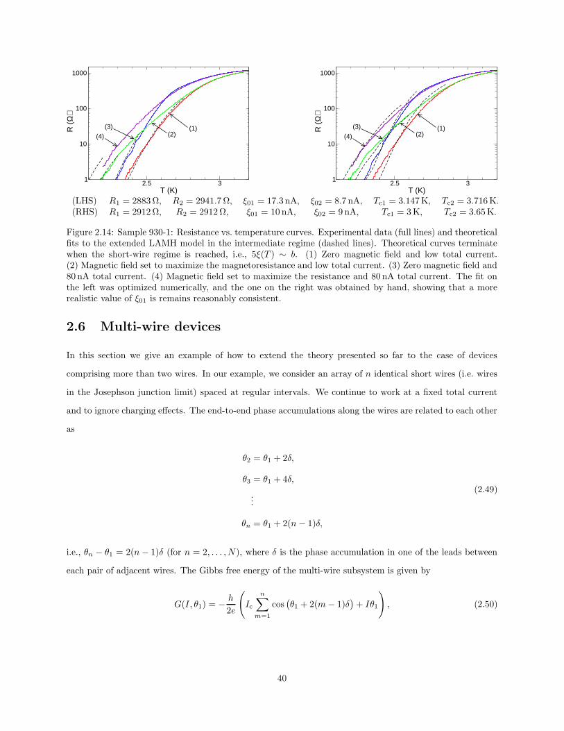
2.5 3T (K)

1

10

100

1000R

(Ω

)

(1)(2)

(3)

(4)

2.5 3T (K)

1

10

100

1000

R (

Ω)

(1)(2)

(3)

(4)

(LHS) R1 = 2883 Ω, R2 = 2941.7 Ω, ξ01 = 17.3 nA, ξ02 = 8.7 nA, Tc1 = 3.147 K, Tc2 = 3.716 K.(RHS) R1 = 2912 Ω, R2 = 2912 Ω, ξ01 = 10 nA, ξ02 = 9 nA, Tc1 = 3 K, Tc2 = 3.65 K.

Figure 2.14: Sample 930-1: Resistance vs. temperature curves. Experimental data (full lines) and theoreticalfits to the extended LAMH model in the intermediate regime (dashed lines). Theoretical curves terminatewhen the short-wire regime is reached, i.e., 5ξ(T ) ∼ b. (1) Zero magnetic field and low total current.(2) Magnetic field set to maximize the magnetoresistance and low total current. (3) Zero magnetic field and80 nA total current. (4) Magnetic field set to maximize the resistance and 80 nA total current. The fit onthe left was optimized numerically, and the one on the right was obtained by hand, showing that a morerealistic value of ξ01 is remains reasonably consistent.

2.6 Multi-wire devices

In this section we give an example of how to extend the theory presented so far to the case of devices

comprising more than two wires. In our example, we consider an array of n identical short wires (i.e. wires

in the Josephson junction limit) spaced at regular intervals. We continue to work at a fixed total current

and to ignore charging effects. The end-to-end phase accumulations along the wires are related to each other

as

θ2 = θ1 + 2δ,

θ3 = θ1 + 4δ,

...

θn = θ1 + 2(n− 1)δ,

(2.49)

i.e., θn − θ1 = 2(n− 1)δ (for n = 2, . . . , N), where δ is the phase accumulation in one of the leads between

each pair of adjacent wires. The Gibbs free energy of the multi-wire subsystem is given by

G(I, θ1) = − h

2e

(Ic

n∑

m=1

cos(θ1 + 2(m− 1)δ

)+ Iθ1

), (2.50)

40

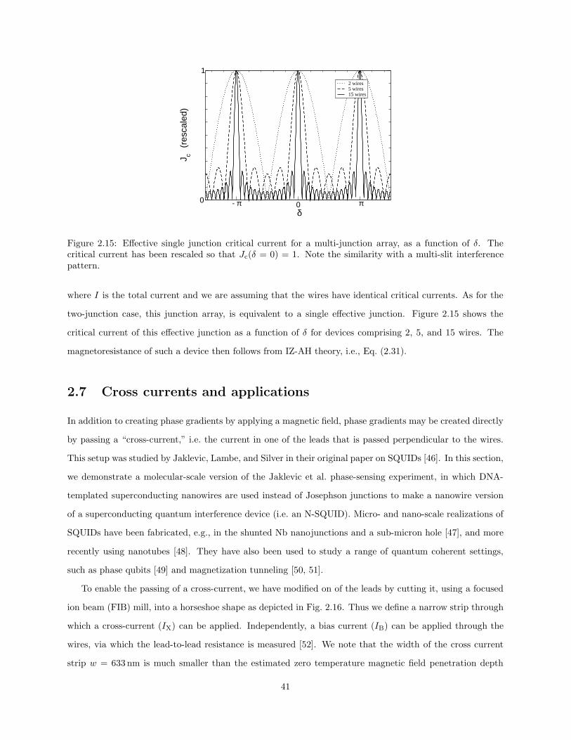
- π 0 π δ

0

1

J c (

resc

aled

)

2 wires5 wires15 wires

Figure 2.15: Effective single junction critical current for a multi-junction array, as a function of δ. Thecritical current has been rescaled so that Jc(δ = 0) = 1. Note the similarity with a multi-slit interferencepattern.

where I is the total current and we are assuming that the wires have identical critical currents. As for the

two-junction case, this junction array, is equivalent to a single effective junction. Figure 2.15 shows the

critical current of this effective junction as a function of δ for devices comprising 2, 5, and 15 wires. The

magnetoresistance of such a device then follows from IZ-AH theory, i.e., Eq. (2.31).

2.7 Cross currents and applications

In addition to creating phase gradients by applying a magnetic field, phase gradients may be created directly

by passing a “cross-current,” i.e. the current in one of the leads that is passed perpendicular to the wires.

This setup was studied by Jaklevic, Lambe, and Silver in their original paper on SQUIDs [46]. In this section,

we demonstrate a molecular-scale version of the Jaklevic et al. phase-sensing experiment, in which DNA-

templated superconducting nanowires are used instead of Josephson junctions to make a nanowire version

of a superconducting quantum interference device (i.e. an N-SQUID). Micro- and nano-scale realizations of

SQUIDs have been fabricated, e.g., in the shunted Nb nanojunctions and a sub-micron hole [47], and more

recently using nanotubes [48]. They have also been used to study a range of quantum coherent settings,

such as phase qubits [49] and magnetization tunneling [50, 51].

To enable the passing of a cross-current, we have modified on of the leads by cutting it, using a focused

ion beam (FIB) mill, into a horseshoe shape as depicted in Fig. 2.16. Thus we define a narrow strip through

which a cross-current (IX) can be applied. Independently, a bias current (IB) can be applied through the

wires, via which the lead-to-lead resistance is measured [52]. We note that the width of the cross current

strip w = 633 nm is much smaller than the estimated zero temperature magnetic field penetration depth

41

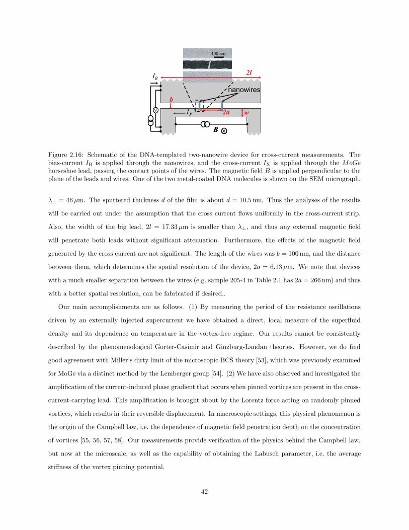
Figure 2.16: Schematic of the DNA-templated two-nanowire device for cross-current measurements. Thebias-current IB is applied through the nanowires, and the cross-current IX is applied through the MoGehorseshoe lead, passing the contact points of the wires. The magnetic field B is applied perpendicular to theplane of the leads and wires. One of the two metal-coated DNA molecules is shown on the SEM micrograph.

λ⊥ = 46µm. The sputtered thickness d of the film is about d = 10.5 nm. Thus the analyses of the results

will be carried out under the assumption that the cross current flows uniformly in the cross-current strip.

Also, the width of the big lead, 2l = 17.33µm is smaller than λ⊥, and thus any external magnetic field

will penetrate both leads without significant attenuation. Furthermore, the effects of the magnetic field

generated by the cross current are not significant. The length of the wires was b = 100 nm, and the distance

between them, which determines the spatial resolution of the device, 2a = 6.13µm. We note that devices

with a much smaller separation between the wires (e.g. sample 205-4 in Table 2.1 has 2a = 266 nm) and thus

with a better spatial resolution, can be fabricated if desired..

Our main accomplishments are as follows. (1) By measuring the period of the resistance oscillations

driven by an externally injected supercurrent we have obtained a direct, local measure of the superfluid

density and its dependence on temperature in the vortex-free regime. Our results cannot be consistently

described by the phenomenological Gorter-Casimir and Ginzburg-Landau theories. However, we do find

good agreement with Miller’s dirty limit of the microscopic BCS theory [53], which was previously examined

for MoGe via a distinct method by the Lemberger group [54]. (2) We have also observed and investigated the

amplification of the current-induced phase gradient that occurs when pinned vortices are present in the cross-

current-carrying lead. This amplification is brought about by the Lorentz force acting on randomly pinned

vortices, which results in their reversible displacement. In macroscopic settings, this physical phenomenon is

the origin of the Campbell law, i.e. the dependence of magnetic field penetration depth on the concentration

of vortices [55, 56, 57, 58]. Our measurements provide verification of the physics behind the Campbell law,

but now at the microscale, as well as the capability of obtaining the Labusch parameter, i.e. the average

stiffness of the vortex pinning potential.

42

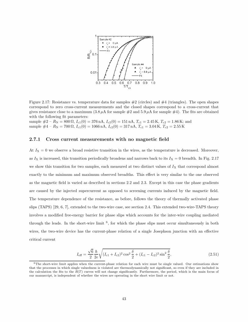
Figure 2.17: Resistance vs. temperature data for samples #2 (circles) and #4 (triangles). The open shapescorrespond to zero cross-current measurements and the closed shapes correspond to a cross-current thatgives resistance close to a maximum (3.8µA for sample #2 and 5.9µA for sample #4). The fits are obtainedwith the following fit parameters:sample #2 – RN = 800 Ω, Ic1(0) = 376 nA, Ic2(0) = 151 nA, Tc1 = 2.45 K, Tc2 = 1.86 K; andsample #4 – RN = 700 Ω, Ic1(0) = 1066 nA, Ic2(0) = 317 nA, Tc1 = 3.04 K, Tc2 = 2.55 K

2.7.1 Cross current measurements with no magnetic field

At IX = 0 we observe a broad resistive transition in the wires, as the temperature is decreased. Moreover,

as IX is increased, this transition periodically broadens and narrows back to its IX = 0 breadth. In Fig. 2.17

we show this transition for two samples, each measured at two distinct values of IX that correspond almost

exactly to the minimum and maximum observed breadths. This effect is very similar to the one observed

as the magnetic field is varied as described in sections 2.2 and 2.3. Except in this case the phase gradients

are caused by the injected supercurrent as opposed to screening currents induced by the magnetic field.

The temperature dependence of the resistance, as before, follows the theory of thermally activated phase

slips (TAPS) [29, 6, 7], extended to the two-wire case, see section 2.4. This extended two-wire-TAPS theory

involves a modified free-energy barrier for phase slips which accounts for the inter-wire coupling mediated

through the leads. In the short-wire limit 6, for which the phase slips must occur simultaneously in both

wires, the two-wire device has the current-phase relation of a single Josephson junction with an effective

critical current

Ieff =

√6

2

~

2e

√(Ic1 + Ic2)2 cos2

δ

2+ (Ic1 − Ic2)2 sin2 δ

2, (2.51)

6The short-wire limit applies when the current-phase relation for each wire must be single valued. Our estimations showthat the processes in which single valuedness is violated are thermodynamically not significant, so even if they are included inthe calculation the fits to the R(T ) curves will not change significantly. Furthermore, the period, which is the main focus ofour manuscript, is independent of whether the wires are operating in the short wire limit or not.

43

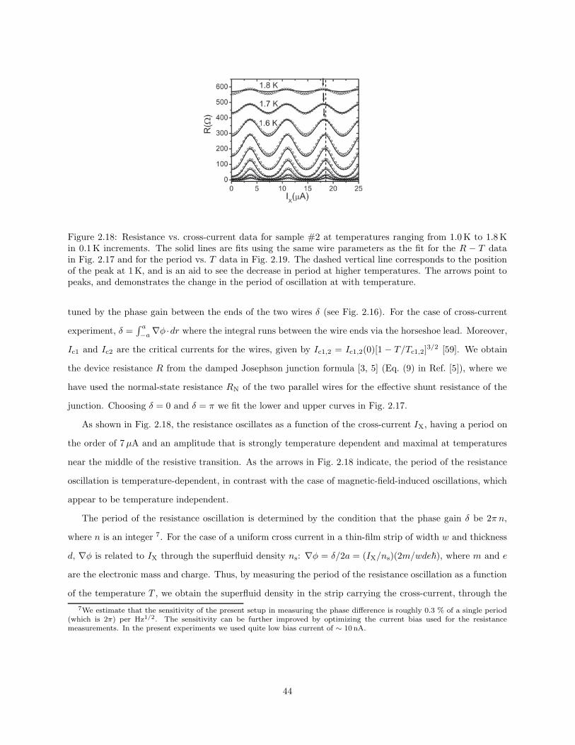
Figure 2.18: Resistance vs. cross-current data for sample #2 at temperatures ranging from 1.0 K to 1.8 Kin 0.1 K increments. The solid lines are fits using the same wire parameters as the fit for the R − T datain Fig. 2.17 and for the period vs. T data in Fig. 2.19. The dashed vertical line corresponds to the positionof the peak at 1 K, and is an aid to see the decrease in period at higher temperatures. The arrows point topeaks, and demonstrates the change in the period of oscillation at with temperature.

tuned by the phase gain between the ends of the two wires δ (see Fig. 2.16). For the case of cross-current

experiment, δ =∫ a

−a∇φ ·dr where the integral runs between the wire ends via the horseshoe lead. Moreover,

Ic1 and Ic2 are the critical currents for the wires, given by Ic1,2 = Ic1,2(0)[1 − T/Tc1,2]3/2 [59]. We obtain

the device resistance R from the damped Josephson junction formula [3, 5] (Eq. (9) in Ref. [5]), where we

have used the normal-state resistance RN of the two parallel wires for the effective shunt resistance of the

junction. Choosing δ = 0 and δ = π we fit the lower and upper curves in Fig. 2.17.

As shown in Fig. 2.18, the resistance oscillates as a function of the cross-current IX, having a period on

the order of 7µA and an amplitude that is strongly temperature dependent and maximal at temperatures

near the middle of the resistive transition. As the arrows in Fig. 2.18 indicate, the period of the resistance

oscillation is temperature-dependent, in contrast with the case of magnetic-field-induced oscillations, which

appear to be temperature independent.

The period of the resistance oscillation is determined by the condition that the phase gain δ be 2π n,

where n is an integer 7. For the case of a uniform cross current in a thin-film strip of width w and thickness

d, ∇φ is related to IX through the superfluid density ns: ∇φ = δ/2a = (IX/ns)(2m/wde~), where m and e

are the electronic mass and charge. Thus, by measuring the period of the resistance oscillation as a function

of the temperature T , we obtain the superfluid density in the strip carrying the cross-current, through the

7We estimate that the sensitivity of the present setup in measuring the phase difference is roughly 0.3 % of a single period(which is 2π) per Hz1/2. The sensitivity can be further improved by optimizing the current bias used for the resistancemeasurements. In the present experiments we used quite low bias current of ∼ 10 nA.

44

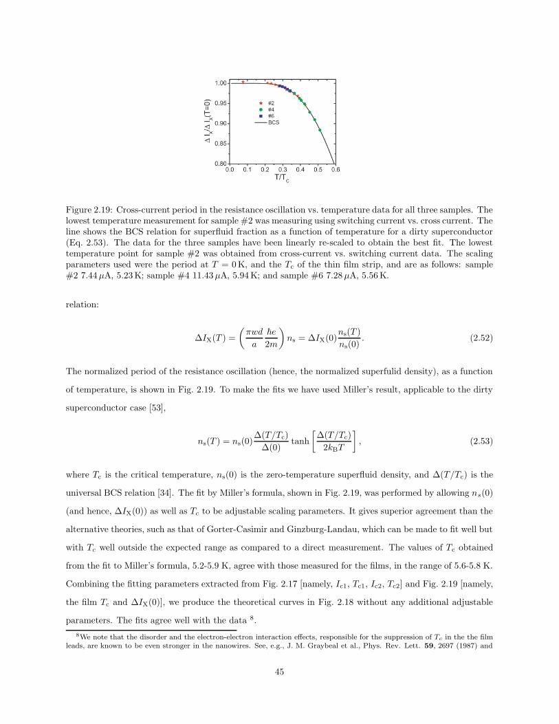
Figure 2.19: Cross-current period in the resistance oscillation vs. temperature data for all three samples. Thelowest temperature measurement for sample #2 was measuring using switching current vs. cross current. Theline shows the BCS relation for superfluid fraction as a function of temperature for a dirty superconductor(Eq. 2.53). The data for the three samples have been linearly re-scaled to obtain the best fit. The lowesttemperature point for sample #2 was obtained from cross-current vs. switching current data. The scalingparameters used were the period at T = 0 K, and the Tc of the thin film strip, and are as follows: sample#2 7.44µA, 5.23 K; sample #4 11.43µA, 5.94 K; and sample #6 7.28µA, 5.56 K.

relation:

∆IX(T ) =

(πwd

a

~e

2m

)ns = ∆IX(0)

ns(T )

ns(0). (2.52)

The normalized period of the resistance oscillation (hence, the normalized superfulid density), as a function

of temperature, is shown in Fig. 2.19. To make the fits we have used Miller’s result, applicable to the dirty

superconductor case [53],

ns(T ) = ns(0)∆(T/Tc)

∆(0)tanh

[∆(T/Tc)

2kBT

], (2.53)

where Tc is the critical temperature, ns(0) is the zero-temperature superfluid density, and ∆(T/Tc) is the

universal BCS relation [34]. The fit by Miller’s formula, shown in Fig. 2.19, was performed by allowing ns(0)

(and hence, ∆IX(0)) as well as Tc to be adjustable scaling parameters. It gives superior agreement than the

alternative theories, such as that of Gorter-Casimir and Ginzburg-Landau, which can be made to fit well but

with Tc well outside the expected range as compared to a direct measurement. The values of Tc obtained

from the fit to Miller’s formula, 5.2-5.9 K, agree with those measured for the films, in the range of 5.6-5.8 K.

Combining the fitting parameters extracted from Fig. 2.17 [namely, Ic1, Tc1, Ic2, Tc2] and Fig. 2.19 [namely,

the film Tc and ∆IX(0)], we produce the theoretical curves in Fig. 2.18 without any additional adjustable

parameters. The fits agree well with the data 8.

8We note that the disorder and the electron-electron interaction effects, responsible for the suppression of Tc in the the filmleads, are known to be even stronger in the nanowires. See, e.g., J. M. Graybeal et al., Phys. Rev. Lett. 59, 2697 (1987) and

45

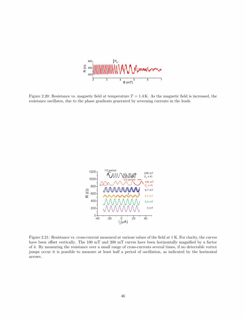
Figure 2.20: Resistance vs. magnetic field at temperature T = 1.4 K. As the magnetic field is increased, theresistance oscillates, due to the phase gradients generated by screening currents in the leads.

Figure 2.21: Resistance vs. cross-current measured at various values of the field at 1 K. For clarity, the curveshave been offset vertically. The 100 mT and 200 mT curves have been horizontally magnified by a factorof 4. By measuring the resistance over a small range of cross-currents several times, if no detectable vortexjumps occur it is possible to measure at least half a period of oscillation, as indicated by the horizontalarrows.

46

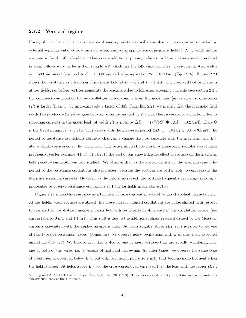
2.7.2 Vorticial regime

Having shown that our device is capable of sensing resistance oscillations due to phase gradients created by

external supercurrents, we now turn our attention to the application of magnetic fields & Hc1, which induce

vortices in the thin-film leads and thus create additional phase gradients. All the measurements presented

in what follows were performed on sample #2, which has the following geometry: cross-current strip width

w = 633 nm, uncut lead width 2l = 17330 nm, and wire separation 2a = 6133 nm (Fig. 2.16). Figure 2.20

shows the resistance as a function of magnetic field at IX = 0 and T = 1.4 K. The observed fast oscillations

at low fields, i.e. before vortices penetrate the leads, are due to Meissner screening currents (see section 2.3),

the dominant contribution to the oscillation period coming from the uncut lead [as its shortest dimension

(2l) is larger (than w) by approximately a factor of 30]. From Eq. 2.21, we predict that the magnetic field

needed to produce a 2π phase gain between wires (separated by 2a) and, thus, a complete oscillation, due to

screening currents in the uncut lead (of width 2l) is given by ∆Bth = (π2/8G)(Φ0/2al) = 102.5µT, where G

is the Catalan number ≈ 0.916. This agrees with the measured period ∆Bexp = 101.8µT. At ∼ 3.5 mT, the

period of resistance oscillations abruptly changes, a change that we associate with the magnetic field Hc1

above which vortices enter the uncut lead. The penetration of vortices into mesoscopic samples was studied

previously, see for example [43, 60, 61], but to the best of our knowledge the effect of vortices on the magnetic

field penetration depth was not studied. We observe that as the vortex density in the lead increases, the

period of the resistance oscillations also increases, because the vortices are better able to compensate the

Meissner screening currents. However, as the field is increased, the vortices frequently rearrange, making it

impossible to observe resistance oscillations at 1.4 K for fields much above Hc1.

Figure 2.21 shows the resistance as a function of cross-current at several values of applied magnetic field.

At low fields, when vortices are absent, the cross-current induced oscillations are phase shifted with respect

to one another for distinct magnetic fields but with no detectable difference in the oscillation period (see

curves labeled 0 mT and 3.4 mT). This shift is due to the additional phase gradient caused by the Meissner

currents associated with the applied magnetic field. At fields slightly above Hc1, it is possible to see one

of two types of resistance traces. Sometimes, we observe noisy oscillations with a smaller than expected

amplitude (4.5 mT). We believe that this is due to one or more vortices that are rapidly wandering near

one or both of the wires, i.e. a version of motional narrowing. At other times, we observe the same type

of oscillation as observed below Hc1, but with occasional jumps (6.7 mT) that become more frequent when

the field is larger. At fields above Hc1 for the cross-current carrying lead (i.e. the lead with the larger Hc1),

Y. Oreg and A. M. Finkel’stein, Phys. Rev. Lett. 83, 191 (1999). Thus, as expected, the Tc we obtain for our nanowires issmaller than that of the film leads.

47

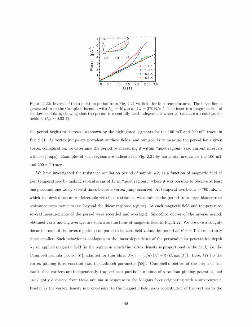
Figure 2.22: Inverse of the oscillation period from Fig. 2.21 vs. field, for four temperatures. The black line isgenerated from the Campbell formula with λ⊥ = 46µm and k = 370 N/m2. The inset is a magnification ofthe low-field data, showing that the period is essentially field independent when vortices are absent (i.e. forfields < Hc1 ∼ 0.02 T).

the period begins to decrease, as shown by the highlighted segments for the 100 mT and 200 mT traces in

Fig. 2.21. As vortex jumps are prevalent at these fields, and our goal is to measure the period for a given

vortex configuration, we determine the period by measuring it within “quiet regions” (i.e. current intervals

with no jumps). Examples of such regions are indicated in Fig. 2.21 by horizontal arrows for the 100 mT

and 200 mT traces.

We have investigated the resistance oscillation period of sample #2, as a function of magnetic field at

four temperatures by making several scans of IX in “quiet regions,” where it was possible to observe at least

one peak and one valley several times before a vortex jump occurred. At temperatures below ∼ 700 mK, at

which the device has an undetectable zero-bias resistance, we obtained the period from large bias-current

resistance measurements (i.e. beyond the linear response regime). At each magnetic field and temperature,

several measurements of the period were recorded and averaged. Smoothed curves of the inverse period,

obtained via a moving average, are shown as functions of magnetic field in Fig. 2.22. We observe a roughly

linear increase of the inverse period; compared to its zero-field value, the period at B = 3 T is some thirty

times smaller. Such behavior is analogous to the linear dependence of the perpendicular penetration depth

λ⊥ on applied magnetic field (in the regime in which the vortex density is proportional to the field), i.e. the

Campbell formula [55, 56, 57], adapted for thin films: λC,⊥ = (1/d)(λ2 + Φ0B/µ0k(T )

). Here, k(T ) is the

vortex pinning force constant (i.e. the Labusch parameter [58]). Campbell’s picture of the origin of this

law is that vortices are independently trapped near parabolic minima of a random pinning potential, and

are slightly displaced from these minima in response to the Magnus force originating with a supercurrent.

Insofar as the vortex density is proportional to the magnetic field, so is contribution of the vortices to the

48

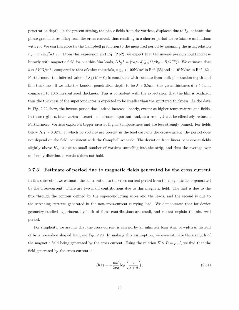
penetration depth. In the present setting, the phase fields from the vortices, displaced due to IX, enhance the

phase gradients resulting from the cross-current, thus resulting in a shorter period for resistance oscillations

with IX. We can therefore tie the Campbell prediction to the measured period by assuming the usual relation

ns = m/µ0e2dλC,⊥. From this expression and Eq. (2.52), we expect that the inverse period should increase

linearly with magnetic field for our thin-film leads, ∆I−1X = (2a/wd)(µ0λ

2/Φ0 +B/k(T )). We estimate that

k ≈ 370N/m2 , compared to that of other materials, e.g., > 100N/m2 in Ref. [55] and ∼ 105N/m2 in Ref. [62].

Furthermore, the inferred value of λ⊥(B = 0) is consistent with estmate from bulk penetration depth and

film thickness. If we take the London penetration depth to be λ ≈ 0.5µm, this gives thickness d ≈ 5.4 nm,

compared to 10.5 nm sputtered thickness. This is consistent with the expectation that the film is oxidized,

thus the thickness of the superconductor is expected to be smaller than the sputtered thickness. As the data

in Fig. 2.22 show, the inverse period does indeed increase linearly, except at higher temperatures and fields.

In these regimes, inter-vortex interactions become important, and, as a result, k can be effectively reduced.

Furthermore, vortices explore a bigger area at higher temperatures and are less strongly pinned. For fields

below Hc1 ∼ 0.02 T, at which no vortices are present in the lead carrying the cross-current, the period does

not depend on the field, consistent with the Campbell scenario. The deviation from linear behavior at fields

slightly above Hc1 is due to small number of vortices tunneling into the strip, and thus the average over

uniformly distributed vortices does not hold.

2.7.3 Estimate of period due to magnetic fields generated by the cross current

In this subsection we estimate the contribution to the cross-current period from the magnetic fields generated

by the cross-current. There are two main contributions due to this magnetic field. The first is due to the

flux through the contour defined by the superconducting wires and the leads, and the second is due to

the screening currents generated in the non-cross-current carrying lead. We demonstrate that for device

geometry studied experimentally both of these contributions are small, and cannot explain the observed

period.

For simplicity, we assume that the cross current is carried by an infinitely long strip of width d, instead

of by a horseshoe shaped lead, see Fig. 2.23. In making this assumption, we over-estimate the strength of

the magnetic field being generated by the cross current. Using the relation ∇× B = µ0J , we find that the

field generated by the cross-current is

B(z) = −µ0I

2πdlog

(z

z + d

), (2.54)

49

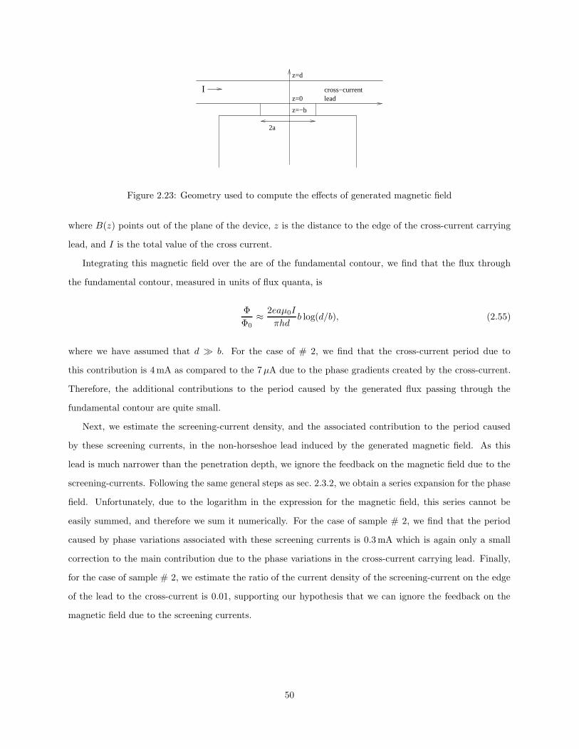
Iz=0

z=−b

z=d

2a

cross−currentlead

Figure 2.23: Geometry used to compute the effects of generated magnetic field

where B(z) points out of the plane of the device, z is the distance to the edge of the cross-current carrying

lead, and I is the total value of the cross current.

Integrating this magnetic field over the are of the fundamental contour, we find that the flux through

the fundamental contour, measured in units of flux quanta, is

Φ

Φ0≈ 2eaµ0I

πhdb log(d/b), (2.55)

where we have assumed that d b. For the case of # 2, we find that the cross-current period due to

this contribution is 4 mA as compared to the 7µA due to the phase gradients created by the cross-current.

Therefore, the additional contributions to the period caused by the generated flux passing through the

fundamental contour are quite small.

Next, we estimate the screening-current density, and the associated contribution to the period caused

by these screening currents, in the non-horseshoe lead induced by the generated magnetic field. As this

lead is much narrower than the penetration depth, we ignore the feedback on the magnetic field due to the

screening-currents. Following the same general steps as sec. 2.3.2, we obtain a series expansion for the phase

field. Unfortunately, due to the logarithm in the expression for the magnetic field, this series cannot be

easily summed, and therefore we sum it numerically. For the case of sample # 2, we find that the period

caused by phase variations associated with these screening currents is 0.3 mA which is again only a small

correction to the main contribution due to the phase variations in the cross-current carrying lead. Finally,

for the case of sample # 2, we estimate the ratio of the current density of the screening-current on the edge

of the lead to the cross-current is 0.01, supporting our hypothesis that we can ignore the feedback on the

magnetic field due to the screening currents.

50

2.8 Concluding remarks

The behavior of mesoscale NQUIDs composed of two superconducing leads connected by a pair of super-

conducting nanowires has been investigated. Magnetoresistance measurements [38] have revealed strong

oscillations in the resistance as a function of magnetic field, and these were found to have anomalously

short periods. The period has been shown to originate in the gradients in the phase of the superconducting

order parameter associated with screening currents generated by the applied magnetic field. The periods

for five distinct devices were calculated, based on their geometry, and were found to fit very well with the

experimental results

The amplitude of the magnetoresistance has been estimated via extensions, to the setting of parallel

superconducting wires, of the IZ-AH theory of intrinsic resistive fluctuations in a current-biased Josephson

junction for the case of short wires and the LAMH theory of intrinsic resistive fluctuations in superconducting

wires for pairs of long wires. In both cases, to make the extensions, it was necessary to take into account

the inter-wire coupling mediated through the leads. For sufficiently long wires, it was found that multiple

metastable states, corresponding to different winding numbers of the phase of the order parameter around

the AB contour, can exist and need to be considered. Accurate fits have been made to the resistance

vs. temperature data at various magnetic fields and for several devices by suitably tuning the critical

temperatures, zero-temperature coherence lengths, and normal-state resistances of the nanowires.

As these device are sensitive to the spatial variations in the phase of the order parameter in the leads,

they may have applications as superconducting phase gradiometers. Such applications may include the

sensing of the presence in the leads of vortices or of supercurrents flowing perpendicular to lead edges. We

also note that our setup can be used to shed light on settings in which local fluctuations of the superfluid

density play a pivotal role, such as those associated with the tail states predicted for superconductors with

magnetic impurities (see e.g. [63]) and those in the junction of two two-dimensional superconducting films

(see e.g. [64]).

51

Chapter 3

Superflow through arrays of nanosized

apertures: disorder, fluctuations,

avalanches, criticality, and other

stories

Superflow in multiply-connected geometries demonstrates rich collective phenomena both in the non-dissipative

(i.e. Josephson) and the dissipative (i.e. irreversible phase-slippage) regimes. In this chapter, and inspired by

recent experiments [65], we construct and analyze a model describing both non-dissipative and dissipative

superflow of a superfluid between two reservoirs through an array of nanosized apertures. The main ingre-

dient of our model are the interactions between superflows through the various apertures, these interactions

being mediated by the superflows in the bulk reservoirs. In addition, for the case of the dissipative regime,

we add aperture-specific (i.e. quenched) disorder to describe the variations in the critical velocity in the

various apertures.

In the non-dissipative we find that, due to the inter-aperture couplings, small arrays of apertures act as

a single effective Josephson link having a coupling strength proportional to the number of apertures. More

complex behavior is expected in larger arrays, which are studied via a renormalization-group approach.

In the dissipative regime, phase slips occurring in individual apertures are the source of dissipation. The

interactions amongst the apertures tends to synchronize these phase-slips, whereas the disorder intrinsic to

each aperture tends to desynchronize them. We find that competition between these tendencies leads to a

disorder-driven continuous phase transition, at which a phase-slip avalanche of macroscopic size first occurs.

We describe the critical properties of our model using the Martin-Siggia-Rose formalism, and find that due

to the long range of the interactions, the upper critical dimension for this phase transition is three. We

compute the critical exponents associated with the transition within mean-field approximation as well as

corrections using an expansion around the upper critical dimension.

Recent experiments [66, 67, 68, 65] on the superflow of 4He between two reservoirs coupled via an

array of nanosized apertures, depicted in Fig. 3.1, found that the system passes through several regimes

of temperature, as the temperature is progressively lowered below the critical temperature Tλ of the bulk

52

system’s transition to the superfluid state. Just below Tλ, and for sufficiently small supercurrents, the array

was observed to function as a single effective Josephson junction having an essentially sinusoidal current-

phase relation. For lower temperatures, below roughly a few millikelvin below Tλ, it was observed that the

single-aperture dynamics becomes irreversible. This is due to the dissipative phase-slips that occur whenever

the superflow velocity in an aperture reaches a critical value [69, 31, 70, 6]. At the high-temperature end of

this regime, there is a narrow interval of temperatures, of width roughly 10 mK, within which all apertures

appear to phase-slip simultaneously, and which Sato et al. [65] refer to as the synchronous regime. For lower

temperatures, down to roughly 160 mK below Tλ, it appears that simultaneity in phase-slippage is lost; Sato

et al. refer to this as the asynchronous regime.

The single-aperture dynamics is controlled by the ratio of the temperature-dependent healing length to

the aperture diameter. For the aperture geometries used in the recent experiments, this ratio can be tuned

to be either very large or very small by varying the temperature. We shall consider two limits, (1) the

high-temperature limit, in which the healing length exceeds the aperture size and the dynamics is reversible,

and the current-phase relation is sinusoidal; (2) the low-temperature limit, in which the aperture size exceeds

the healing length, the dynamics is dissipative, and the current-phase relation is saw-tooth-like (linear, with

sharp, periodic drops). In the low temperature regime, the sharp drops of the supercurrent occur whenever

the supercurrent exceeds an aperture-dependent critical current, and the superflow in the aperture suffers

a phase slip. In both regimes, the long-range nature of inter-aperture interaction mediated by the bulk

superfluids plays an essential role.

For the case of 4He it is known that a single aperture operating in the Josephson regime always has

weak Josephson coupling as compared to thermal fluctuations (EJ < kBT ) [71]. We find that in the high-

temperature regime, due to the long range of the interactions, the effective Josephson coupling between

the reservoirs is proportional to the number of apertures, at least for sufficiently small arrays, supporting

the conclusions of Ref. [72]. However, the effective coupling is suppressed by a factor arising from thermal

fluctuations.

In the low-temperature regime, when dissipation sets in, the dynamics becomes more complex, due to the

disorder associated with the aperture-to-aperture variability of the critical currents. Specifically, the inter-

aperture interactions may lead to an avalanching behavior, in which a phase-slip in one aperture triggers

phase-slips in one or more of its neighbors. We show that this avalanching phenomenon is analogous to

ones observed in disparate physical systems, such as sliding tectonic plates [73], random-field magnets [74],

and solids with disorder-pinned charge-density waves (CDWs) [75, 76], that feature competition between

quenched disorder and interactions. We shall demonstrate a particular kinship to the soft-spin version of the

53

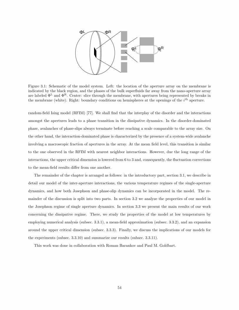
φiL

ΦL

φiR

ΦR

Figure 3.1: Schematic of the model system. Left: the location of the aperture array on the membrane isindicated by the black region, and the phases of the bulk superfluids far away from the nano-aperture arrayare labeled ΦL and ΦR. Center: slice through the membrane, with apertures being represented by breaks inthe membrane (white). Right: boundary conditions on hemispheres at the openings of the ith aperture.

random-field Ising model (RFIM) [77]. We shall find that the interplay of the disorder and the interactions

amongst the apertures leads to a phase transition in the dissipative dynamics. In the disorder-dominated

phase, avalanches of phase-slips always terminate before reaching a scale comparable to the array size. On

the other hand, the interaction-dominated phase is characterized by the presence of a system-wide avalanche

involving a macroscopic fraction of apertures in the array. At the mean field level, this transition is similar

to the one observed in the RFIM with nearest neighbor interactions. However, due the long range of the

interactions, the upper critical dimension is lowered from 6 to 3 and, consequently, the fluctuation corrections

to the mean-field results differ from one another.

The remainder of the chapter is arranged as follows: in the introductory part, section 3.1, we describe in

detail our model of the inter-aperture interactions, the various temperature regimes of the single-aperture

dynamics, and how both Josephson and phase-slip dynamics can be incorporated in the model. The re-

mainder of the discussion is split into two parts. In section 3.2 we analyze the properties of our model in

the Josephson regime of single aperture dynamics. In section 3.3 we present the main results of our work

concerning the dissipative regime. There, we study the properties of the model at low temperatures by

employing numerical analysis (subsec. 3.3.1), a mean-field approximation (subsec. 3.3.2), and an expansion

around the upper critical dimension (subsec. 3.3.3). Finally, we discuss the implications of our models for

the experiments (subsec. 3.3.10) and summarize our results (subsec. 3.3.11).

This work was done in collaboration with Roman Barankov and Paul M. Goldbart.

54

3.1 Introduction

The geometry of the system we wish to describe consists of two large reservoirs of superfluid, separated by a

rigid barrier. Embedded in this barrier is an array of apertures, as shown in Fig. 3.1. We shall specialize to

the case of an N ×N array of apertures, each aperture having length d and radius r0, centered at the sites of

a square lattice of lattice parameter `. It is straightforward to extend our analysis to other array geometries.

It is convenient to regard the superfluid system as comprising three components: two are bulk components

[i.e., the left (L) and right (R) reservoirs]; the third consists of the superfluid inside the apertures. We shall

describe the state of the bulk helium in terms of the phase fields of the superfluid order-parameter. In doing

this we are neglecting effects of amplitude excitations of the order parameter, including vortices, within the

bulk. In contrast, within the apertures we shall retain both amplitude and phase degrees of freedom. We

imagine controlling the system by specifying the phases ΦL/R on surfaces in the bulk superfluids far from

the array of nanoapertures (see Fig. 3.1). We believe that this level of description allows us to capture

the following important elements: (a) apertures that exhibit Josephson dynamics in the high temperature

regime and dissipative dynamics due to narrow-wire-like meta stable states, these states being connected

by phases slips, in the low temperature regime; and (b) interactions mediated through the bulk superfluid

in the two reservoirs, which couple pairs of apertures to one another and also couple the apertures to the

control phases ΦL/R.

We can consider two possible ways to drive the system: either by fixing the total current through the

aperture array or the chemical potential difference ∆µ across it. We shall focus on the second strategy, which

amounts to fixing the rate of change of the control phase difference ΦL − ΦR via the Josephson-Anderson

relation

ΦL − ΦR =∆µ

~t, (3.1)

where t is the time that has passed from the moment when ∆µ was first applied. Fixing ∆µ corresponds

to the typical experimental setup in experiments on superfluid helium [78]. If we wish to fix the total

current, as is typical for experiments on superconductors, we can perform a Legendre transform to change

the independent variable from the control phase difference to the total current [30].

We separate the description of the bulk superfluid from the superfluid inside the apertures by specifying

the phases in the vicinity of the aperture openings. That is for ith aperture we specify the phases in the

55

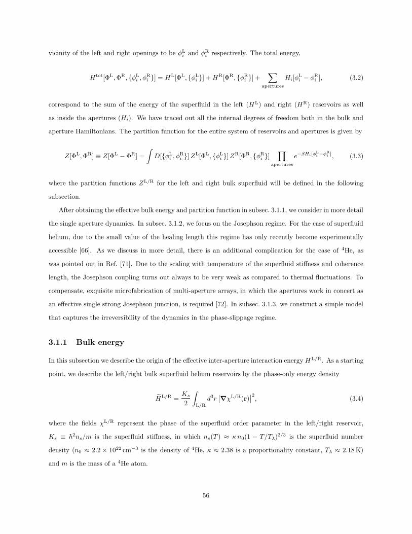
vicinity of the left and right openings to be φLi and φR

i respectively. The total energy,

Htot[ΦL,ΦR, φLi , φ

Ri ] = HL[ΦL, φL

i ] +HR[ΦR, φRi ] +

∑

apertures

Hi[φLi − φR

i ], (3.2)

correspond to the sum of the energy of the superfluid in the left (HL) and right (HR) reservoirs as well

as inside the apertures (Hi). We have traced out all the internal degrees of freedom both in the bulk and

aperture Hamiltonians. The partition function for the entire system of reservoirs and apertures is given by

Z[ΦL,ΦR] ≡ Z[ΦL − ΦR] =

∫D[φL

i , φRi ]ZL[ΦL, φL

i ]ZR[ΦR, φRi ]

∏

apertures

e−βHi[φLi −φR

i ], (3.3)

where the partition functions ZL/R for the left and right bulk superfluid will be defined in the following

subsection.

After obtaining the effective bulk energy and partition function in subsec. 3.1.1, we consider in more detail

the single aperture dynamics. In subsec. 3.1.2, we focus on the Josephson regime. For the case of superfluid

helium, due to the small value of the healing length this regime has only recently become experimentally

accessible [66]. As we discuss in more detail, there is an additional complication for the case of 4He, as

was pointed out in Ref. [71]. Due to the scaling with temperature of the superfluid stiffness and coherence

length, the Josephson coupling turns out always to be very weak as compared to thermal fluctuations. To

compensate, exquisite microfabrication of multi-aperture arrays, in which the apertures work in concert as

an effective single strong Josephson junction, is required [72]. In subsec. 3.1.3, we construct a simple model

that captures the irreversibility of the dynamics in the phase-slippage regime.

3.1.1 Bulk energy

In this subsection we describe the origin of the effective inter-aperture interaction energy HL/R. As a starting

point, we describe the left/right bulk superfluid helium reservoirs by the phase-only energy density

HL/R =Ks

2

∫

L/R

d3r∣∣∇χL/R(r)

∣∣2, (3.4)

where the fields χL/R represent the phase of the superfluid order parameter in the left/right reservoir,

Ks ≡ ~2ns/m is the superfluid stiffness, in which ns(T ) ≈ κn0(1 − T/Tλ)2/3 is the superfluid number

density (n0 ≈ 2.2 × 1022 cm−3 is the density of 4He, κ ≈ 2.38 is a proportionality constant, Tλ ≈ 2.18 K)

and m is the mass of a 4He atom.

56

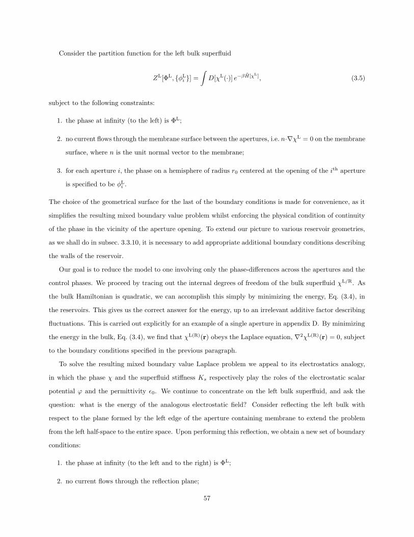
Consider the partition function for the left bulk superfluid

ZL[ΦL, φLi ] =

∫D[χL(·)] e−βH[χL], (3.5)

subject to the following constraints:

1. the phase at infinity (to the left) is ΦL;

2. no current flows through the membrane surface between the apertures, i.e. n·∇χL = 0 on the membrane

surface, where n is the unit normal vector to the membrane;

3. for each aperture i, the phase on a hemisphere of radius r0 centered at the opening of the ith aperture

is specified to be φLi .

The choice of the geometrical surface for the last of the boundary conditions is made for convenience, as it

simplifies the resulting mixed boundary value problem whilst enforcing the physical condition of continuity

of the phase in the vicinity of the aperture opening. To extend our picture to various reservoir geometries,

as we shall do in subsec. 3.3.10, it is necessary to add appropriate additional boundary conditions describing

the walls of the reservoir.

Our goal is to reduce the model to one involving only the phase-differences across the apertures and the

control phases. We proceed by tracing out the internal degrees of freedom of the bulk superfluid χL/R. As

the bulk Hamiltonian is quadratic, we can accomplish this simply by minimizing the energy, Eq. (3.4), in

the reservoirs. This gives us the correct answer for the energy, up to an irrelevant additive factor describing

fluctuations. This is carried out explicitly for an example of a single aperture in appendix D. By minimizing

the energy in the bulk, Eq. (3.4), we find that χL(R)(r) obeys the Laplace equation, ∇2χL(R)(r) = 0, subject

to the boundary conditions specified in the previous paragraph.

To solve the resulting mixed boundary value Laplace problem we appeal to its electrostatics analogy,

in which the phase χ and the superfluid stiffness Ks respectively play the roles of the electrostatic scalar

potential ϕ and the permittivity ε0. We continue to concentrate on the left bulk superfluid, and ask the

question: what is the energy of the analogous electrostatic field? Consider reflecting the left bulk with

respect to the plane formed by the left edge of the aperture containing membrane to extend the problem

from the left half-space to the entire space. Upon performing this reflection, we obtain a new set of boundary

conditions:

1. the phase at infinity (to the left and to the right) is ΦL;

2. no current flows through the reflection plane;

57

Electrostatic

analogy

Figure 3.2: Left: schematic of the mixed boundary value problem for the superflows in the left reservoir.The solid block represents the membrane and the breaks in it represent the apertures. The surface labeledΦL represents the boundary condition on the phase of the order parameter far away from the aperture array.The hemi-spherical surfaces labeled φ1, φ2, and φ3 represent the boundary condition on the phase of theorder parameter on these imaginary surfaces located at the aperture openings. Right: schematic for theanalogous electrostatics boundary value problem. In the picture on the right, the picture on the left hasbeen duplicated and one copy reflected across the plane formed by the left edge of the aperture containingmembrane. The hemispherical surfaces of constant phase at the aperture openings on the left have beenreplaced by equipotential spheres (spherical capacitors) on the right. Similarly, the boundary condition atinfinity to the left has been replicated on the right.

3. for each aperture i, the phase on a sphere of radius r0, formed from the original hemisphere and its

reflection is specified to be φLi .

These boundary condition specify an electrostatics problem to compute the energy of the electric field

produced by an array of conductive spheres (spherical capacitors) held at fixed potentials, see Fig. 3.2.

Condition (2.) is automatically satisfied due to the symmetry of the problem. To compute the energy, in

terms of the boundary data, we apply the divergence theorem to Eq. (3.4) to obtain the energy in terms of

a surface integral:

HL =Ks

2

∫

∂ L

dS · χL∇χL − Ks

2

∫

L

d3r χL∇2χL, (3.6)

where the volume (i.e. the last) term vanishes upon minimization (computing the variation of HL with respect

to χL, we find that the minimum-energy configuration χL obeys ∇2χL = 0). To simplify the evaluation of

the surface integral we make use of the fact that the energy is invariant under global shifts of the potential.

Thus, we lower all potentials by ΦL, which eliminates the contribution from the (left and right) surfaces at

infinity. What remains are the contributions from the surfaces of the spherical capacitors, which give the

effective energy

HL =1

2

∑

apertures

(φLi − ΦL) qi, (3.7)

which is a well known relation in electrostatics. Here, for each aperture i, the phase χL takes the constant

value φLi (shifted to φL

i − ΦL) on the associated spherical surface, and the remaining surface integrals have

58

been replaced (via the analogue of Gauss’s law) by the supercurrent out of the surface which is the analogue

of the charge enclosed qi. For aperture i this “charge” is qi ≡ Ks

∫dS ·∇χL, where the integral is taken over

the spherical surface. What remains is to determine the charges qi. To do this, we consider the ith sphere:

in the limit ` r0, where ` is the distance between the closest apertures (i.e. ignoring di- and higher-order

charge-multipoles), the potential on its surface obeys

Ks

(φL

i − ΦL)

=∑

j

C−1ij qj , (3.8a)

C−1ij ≡

δij4π r0

+1− δij4π |rij |

, (3.8b)

where |rij | is the distance between the ith and jth aperture (sphere) centers, and Cij is the analogue of the

capacitance matrix . By solving Eq. (3.8a) for the qi’s and eliminating them from Eq. (3.7) (and dividing

by two, as we want the energy of the left bulk only), we arrive at the energy of the superfluid in the left

reservoir.

HL =Ks

4

∑

ij

(φLi − ΦL)Cij (φL

j − ΦL). (3.9)

In general the structure of the Cij matrix is as follows: the diagonal elements Cii ∼ 4πr0 are positive,

while the off diagonal elements are negative, with the property∑

j Cij > 0. For an infinite regular array

of apertures, Cij may be obtained by Fourier transforming C−1ij , inverting, and anti-Fourier transforming.

Upon performing this procedure, we find that the Cij matrix has the following asymptotes

Cij ∼

r20/|rij |, |rij | `2/r0

`4/|rij |3, |rij | `2/r0

. (3.10)

The inter-aperture coupling falls off as 1/r for aperture that are close together, and as 1/r3 for apertures

that are far apart. The 1/r3 long range nature of the interaction is key for determining the properties of

large aperture arrays. This form of dependence of the inter-aperture coupling on the distance between the

apertures seems to be generally true, based in numerical investigations, as long as the square root of the

total number of apertures satisfies N `/r0. The infinitely large array limit has an the additional property

that∑

j Cij = 0. This property implies the decoupling from the control phase in the bulk, which is sensible

as the problem becomes one-dimensional.

59

3.1.2 Single-aperture dynamics in the Josephson regime

Having obtained the effective energy for the bulk superfluids, we complete the description by specifying the

effective energy of the superfluid in the apertures. In the present subsection we shall concentrate on the

temperature regime in which apertures act as Josephson junctions. In this regime the current-phase relation

for a single aperture is single-valued, and the single aperture energy is given by

Hi = −EJ cos(φLi − φR). (3.11)

The Josephson effect is an important consequence of macroscopic quantum phenomena. In the setting of

superconductors, it was first proposed by Brian Josephson in 1962 [79], and was observed soon thereafter [80,

81]. More recently, the Josephson effect has also been observed between two weakly coupled BEC [82], as

well as in superfluid 3He [83, 84, 78] and 4He [66, 68] weak links.

Being able to observe any sort of Josephson effect in 4He is a serious concern because the Josephson

coupling strength across a single aperture is always smaller than kBT [71]. This may be demonstrated

by the following scaling analysis due to Zimmermann [71, 72], which shows that the maximum Josephson

coupling for a given aperture is independent of its size, and is very small. Consider an aperture having

radius r0 and length (membrane thickness) d. Here, we shall focus on the experimentally relevant situation

of apertures having d ∼ 2r0. Following Ref. [72], the Josephson coupling strength 2EJ is roughly proportional

to the largest kinetic energy achievable within the aperture, i.e.

2EJ ≈ns~

2

2m4

∫|∇φ|2d3x, (3.12)

where ns is the superfluid density, m4 is the mass of a 4He atom, φ is the phase of the order parameter, and

the integral runs over the volume of an aperture. The maximum kinetic energy is achieved when the phase

difference across the aperture is π, for which ∇φ ∼ π/d. To maximize EJ we lower the temperature so as to

maximize the superfluid fraction. However, in order for the aperture to function in the Josephson regime,

we must stop lowering the temperature at the point where the temperature-dependent healing length is

comparable to the aperture diameter. This point defines the temperature Tm, via the relation ξ(Tm) = 2r0.

Below Tm the aperture stops acting as a Josephson junction. Therefore, the maximal Josephson coupling

occurs at the temperature Tm, where it obtains the value EJ ≈ ns(Tm)~2

2m ξ(Tm). Using the scaling relations

near Tλ, i.e. ns ≈ n′0(1− T/Tλ)2/3 and ξ(T ) ≈ ξ0(1− T/Tλ)−2/3, we find that EJ ∼ 0.6 K is independent of

Tm and therefore it is also independent of the aperture size.

60

Due to the fact that ξ0 ∼ 2 × 10−10 m, which is much smaller than the smallest aperture that can be

made, in order for an aperture to operate in the Josephson regime the temperature must be very near the

transition temperature, Tλ = 2.18 K. As EJ < kBT , the Josephson effect is not expected to survive for the

case of a single aperture [34].

3.1.3 Single-aperture dynamics in the phase slippage regime

For single apertures operating in the dissipative regime, observations of single-phase slip events were first

reported in Refs. [85, 83]. The cross-over between the Josephson and the dissipative regimes has been studied

experimentally in Ref. [68]. It was found that as the temperature is lowered, and thus the temperature-

dependent healing length decreased, the sinusoidal current-phase relation becomes distorted into the shape of

a breaking wave. This reflects the development of metastable current-carrying states that first appear when

the healing length becomes commensurate with the aperture size. The switching between these metastable

states occurs through phase-slip processes, which arise from vortex lines crossing the aperture [31].

To account for phase-slippage processes within an aperture we shall use a modified phase-only model

that accounts for the vanishing of the amplitude associated with vortex lines by keeping track of the number

of phase slips that have occurred. Therefore, we take the energy of the superfluid inside the ith aperture to

be

Hi =Ks

2J(φL

i − φRi − 2πni

)2, (3.13)

in which J(≡ π r20/d) accounts for the geometry of the aperture, where d is of the order of the membrane

thickness. The integer ni counts the net number of phase slips that would occur in the ith aperture if

the system were to progress to its present state from a reference state in which the phases were uniform

throughout the system.

We complete the description of our model by specifying the single-aperture dynamics, and thus the

mechanism by which energy is dissipated in the apertures. The superfluid velocity vi in a aperture of thickness

d is defined by the phases at the aperture openings: vi = ~∇φi/m ≈ ~(2φL

i − 2πni

)/dm. Correspondingly,

the current through the aperture is given by

Ii =KsJ

~

(2φL

i − 2πni

). (3.14)

When the velocity through the ith aperture exceeds its critical value vc,i (or, equivalently, φLi − πni exceeds

φc,i), a vortex line nucleates and moves across the aperture, which decreases the phase-difference along a

61

path from the far left, through the ith aperture, to the far right by 2π, whilst the phase-difference along a

path through any other aperture remains unaffected. In our model, we implement this kind of phase-slip

event by sending ni to ni + 1 (assuming all flow is to the left).

The Berkeley group’s experiments are primarily conducted in the temperature regime in which T is close

to Tλ [65]. In this regime, the intrinsic critical velocity is proportional to the superfluid stiffness [85, 70, 6]:

vc(T ) ' ~/mξ(T ) ∝ Ks(T ), (3.15)

where, as before, ξ(T ) ' ξ0(1−T/Tλ)−2/3 is the temperature-dependent superfluid healing length. Extrinsic

effects are known to reduce critical velocities from their intrinsic values. We hypothesize that in the Berkeley

group’s experiments these extrinsic effects originate in atomic-scale roughness of the aperture walls, and play

a pivotal role in generating critical-velocity variability amongst the apertures. This variability is expected

to be temperature dependent, because only roughness on length-scales longer than ξ(T ) can substantially

perturb the order parameter and thus influence the critical velocities. Hence, at higher temperatures the

impact of surface roughness is expected to be weaker and, correspondingly, the distribution of critical

velocities is expected to be narrower. Under this hypothesis, lowering the temperature has the important

effective consequence of increasing the effective disorder 1.

3.1.4 Summary of the model

To summarize, we describe the three components of the system by the total energy

H = HL +HR +∑

i

Hi, (3.16)

where HL/R, given by the Eq. (3.16), describes the superflows in the left/right bulk superfluid and Hi

describes the superflow in the ith aperture and has different functional form in the low-temperature regime

Eq. (3.11) and high-temperature regime Eq. (3.13). We connect the description of the bulk superfluids to

that of the superfluids within the apertures by specifying the phases at the interfaces. That is, in the vicinity

of the aperture openings we specify the phases to be φL/Ri (Fig. 3.1). Having specified φ

L/Ri and ΦL/R, we

can express HL/R through a set of effective couplings between the phases in the vicinities of the various

apertures and the control phases. For convenience, we set ΦR = −ΦL by a suitable choice of gauge, and

focus on states in which the left and right hand sides of the system are symmetric, so that φRi = −φL

i . In

this case, we need only specify the (L) phases for a full description of the system, which is what we shall do

1Similar ideas have been suggested by Y. Sato and co-workers (private communication (2006)).

62

from now on.

3.2 Analysis of array dynamics in the Josephson regime

In this section, we demonstrate that multiple apertures can cooperate to make the Josephson effect in 4He

observable. The main result of this section is that for small arrays of apertures the total effective Josephson

coupling EtotJ is given by

EtotJ = N2EJ , (3.17)

where EJ is the effective single-aperture coupling and N 2 is the total number of apertures. Our result agrees

with that of Ref. [72], in that the total coupling is proportional to the number of apertures. However, in

contrast to the conclusions of Ref. [72], we find that the phases in the vicinity of the aperture openings

always suffer strong thermal fluctuations and are not locked together. As a result, Eq. (3.17) features an

effective single aperture coupling that accounts for the thermal fluctuations EJ instead of the bare coupling

EJ . Finally, for large arrays, due to correlated fluctuations, the total coupling grows slower than the array

size.

We proceed by: (1) identifying a model for the energetics of the superflows through the apertures and the

bulk superfluid reservoirs, making the approximation that the superfluid in the vicinity of the aperture array

comes into equilibrium much more quickly than the phase difference between the bulk superfluids evolves

in time; (2) integrating out the fluctuations in the bulk superfluids; and (3) obtaining the effective coupling

between the bulk superfluids by tracing over the configurations of the phases in the vicinity of the aperture

openings using both analytical and numerical approaches.

We begin by assuming that the bulk reservoirs are large and three dimensional, and therefore there is a

well-defined phase difference between them. Furthermore, we shall assume that this phase difference evolves

slowly in time, such that the superfluid in the vicinity of the apertures is always in thermal equilibrium,

subject to the constraint that deep within the bulk the phase approaches ΦL/R in the left/right reservoir.

The goal is to obtain the effective free energy of the superfluid in the apertures and in the bulk reservoirs

as a function of ∆Φ ≡ ΦL − ΦR, and thus to extract the total Josephson coupling.

63

Following Eq. (3.3), the partition function for a given ∆Φ is

Z[∆Φ] = e−βSeff[∆Φ], (3.18)

Seff[∆Φ] =Ks

2

∑

ij

(φLi − ΦL)Cij(φL

j − ΦL)−EJ

∑

i

cos(2φLi ). (3.19)

Before continuing with a detailed analysis of the model, we pause to demonstrate that, within this model,

the fluctuations of the phase across any individual aperture are large (compared to 2π). The phase φi across

the ith aperture is constrained from fluctuating by both the EJ (Josephson) term and by its coupling to the

other apertures and to the phase deep in the bulk via the Cij term. The fluctuations across a given aperture

will be weakest when the two terms constraining it are largest. Assuming that we have already tuned the

temperature so as to maximize EJ while remaining in the Josephson regime of single aperture dynamics, we

concentrate on tuning the Cij term. Largest constraint by the Cij term is achieved for the case of a large

array, with all the φj ’s except the one of interest frozen so that they cannot fluctuate. Locking all the other

phases to zero (or a multiple of π to ensure that both the Josephson term and the inter-aperture coupling

term have the same minimum), we find that the energy associated with fluctuations of the phase across ith

aperture is

Ks

2Ciiφ

2i +EJ cosφi, (3.20)

where the first term is approximately 2πKsr0φ2i and the second term is approximately ∼ Ksπr0/d cos(φi).

For the geometry of interest, 2r0 ∼ d, we see that the presence of the other apertures in the array only changes

the total energy for fluctuations of φi → ±2π by a small factor. However, from the form of Eq. (3.20) we

see that the aperture is constrained to fluctuate around the point φi = 0. We believe that this observation

is the key to understanding the observation of the Josephson effect in aperture array. Furthermore, due to

the long range order present in superfluid, relaxing the condition that all the other apertures are frozen does

not significantly affect this conclusion.

Next, we integrate over the φi’s, to obtain an effective action (and the associated partition function) for

the phases at infinity. This is hard to do directly, due to the non-linear cosine term. A useful approach is

to replace the cosine potential by the Villian potential. The prescription for doing this is to perform the

following replacement:

eβEJ cos(x) →∞∑

η=−∞e−β

EV2

(x−2πη)2 , (3.21)

64

which produces another periodic potential with similar amplitude. This mapping is only approximate,

however, physical results should remain unchanged provided that we correctly scale the the Villian potential

relative to the cosine potential (i.e. conserve the amplitude of the energy difference between the maximum

and minimum of the potential), which we do using the following (implicit) transformation:

2βEJ =EllipticTheta[3, 0, e−2π2βEV ]

EllipticTheta[2, 0, e−2π2βEV ]. (3.22)

Upon transforming to the Villian potential, we obtain:

Z =

∫D[ΦL]D[φL

i ]∑

ηiexp

−βKs

2

∑

ij

(φLi − ΦL)Cij (φL

j − ΦL) +EV

2

∑

i

(2φLi − 2πηi)

2

, (3.23)

where ηi stands for all possible combinations of the Villian “charges.” We can now perform the integral

over the φLi ’s, to obtain an effective partition function with the Villain charges and ∆Φ as the remaining

degrees of freedom:

Z =

∫D[ΦL]

∑

ηie−βHeff(Φ

L,ηi) (3.24)

Heff(ΦL, ηi) =

−1

4

∑

ij

(ΦLKs

2

∑

k

Cki + 2πEV ηi

)(Ks

4Cij +

EV

2δij

)−1(

ΦLKs

2

∑

m

Cmj + 2πEV ηj

)

(3.25)

+Ks

4(ΦL)2

∑

ij

Cij +EV

2

∑

i

(2πηi)2

. (3.26)

To make further progress, we make the small, well spaced array approximation, i.e. we ignore the off-

diagonal elements of the C−1ij matrix, and approximate the diagonal ones by C−1

ii ≈ 1/4πr0. The effective

action under this assumption becomes

Seff(Φ) = − 1

βlogZ[Φ] = N2EJ

[EV Ks

Ks + 2EV C−1ij

]cos(Φ), (3.27)

where EJ [.] is transformation (3.22) from EV to EJ , and N2 is the total number of apertures. This is clearly

just N2 times the action for a single aperture. Here, EJ ≡ EJ

[EV Ks

Ks+2EV C−1

ij

]plays the role of an effective

coupling, which takes into account the “fringe” fields, i.e. the hydrodynamic flows around the aperture.

Therefore, it is easy to see that whenever N 2 is large enough, the total coupling can exceed the strength of

thermal fluctuations, leading to the Josephson effect using the mechanism described in Ref. [72]. However,

65

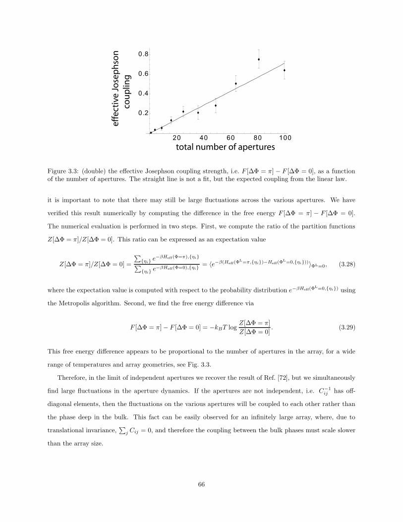
20 40 60 80 100

0.2

0.4

0.6

0.8

total number of apertures

eff

ect

ive

Jo

sep

hso

n

co

up

lin

g

Figure 3.3: (double) the effective Josephson coupling strength, i.e. F [∆Φ = π] − F [∆Φ = 0], as a functionof the number of apertures. The straight line is not a fit, but the expected coupling from the linear law.

it is important to note that there may still be large fluctuations across the various apertures. We have

verified this result numerically by computing the difference in the free energy F [∆Φ = π] − F [∆Φ = 0].

The numerical evaluation is performed in two steps. First, we compute the ratio of the partition functions

Z[∆Φ = π]/Z[∆Φ = 0]. This ratio can be expressed as an expectation value

Z[∆Φ = π]/Z[∆Φ = 0] =

∑ηi e

−βHeff(Φ=π),ηi∑ηi e

−βHeff(Φ=0),ηi = 〈e−β(Heff(ΦL=π,ηi)−Heff(Φ

L=0,ηi))〉ΦL=0, (3.28)

where the expectation value is computed with respect to the probability distribution e−βHeff(ΦL=0,ηi) using

the Metropolis algorithm. Second, we find the free energy difference via

F [∆Φ = π]− F [∆Φ = 0] = −kBT logZ[∆Φ = π]

Z[∆Φ = 0]. (3.29)

This free energy difference appears to be proportional to the number of apertures in the array, for a wide

range of temperatures and array geometries, see Fig. 3.3.

Therefore, in the limit of independent apertures we recover the result of Ref. [72], but we simultaneously

find large fluctuations in the aperture dynamics. If the apertures are not independent, i.e. C−1ij has off-

diagonal elements, then the fluctuations on the various apertures will be coupled to each other rather than

the phase deep in the bulk. This fact can be easily observed for an infinitely large array, where, due to

translational invariance,∑

j Cij = 0, and therefore the coupling between the bulk phases must scale slower

than the array size.

66

3.3 Analysis of the array dynamics in the phase-slippage regime

As we demonstrate later, the quenched disorder in the critical velocities of various apertures dominates

over the disorder associated with thermal noise. Thus, in this section we begin by concentrating on the

quasi-static dynamics of phase-slippage in the aperture array and assume that the impact of thermal noise

on the phase-slippage is negligible.

We work at constant (negative) difference ∆µ in the chemical potential between the reservoirs, so that

the control parameter ΦL evolves linearly in time, according to the Josephson-Anderson relation:

ΦL = −ΦR = −∆µ

2~t. (3.30)

As ΦL − ΦR grows, so do the superfluid velocities through the various apertures, punctuated at regular

intervals by velocity drops associated with phase-slip processes. As, beyond a brief transient interval, the

total energy of the state is periodic in ΦL with period π, the total current through the array must be a

periodic function of time with period given by the Josephson frequency ωJ = ∆µ/~. Due to the randomness

in the critical velocities of the apertures, the velocities in the various apertures do not reach their critical

values simultaneously. Thus, apertures having smaller critical velocities (i.e. weaker apertures) slip first.

We note that immediately after a phase slip in the ith aperture the velocity through it is decreased by

∆v ≡ 2π~/md (i.e. the quantum of superfluid velocity for an aperture having fixed phases at the openings),

i.e. vi → vi −∆v. However, after a very short time (on the order of time it takes sound to cross the array),

the system equilibrates the superflow in the bulk reservoirs and through the various apertures. Therefore,

after this relaxation process is complete, the net drop in the superfluid velocity through the ith aperture is

always less than ∆v. To determine the configuration of the superfluid after a phase slip, we must increment

ni to ni +1 in the description of the energy of the ith aperture Eq. (3.13) (assuming all flow is to the left) and

find the new set of values for all of the φLi ’s by minimizing the total energy, Eq. (3.16). This minimization

results in a decrease of the supervelocity in the ith aperture but an increase in the supervelocity in all of the

other apertures, which pushes them closer to their own critical velocities.

If the distribution of critical velocities is sufficiently narrow, the array may—as we demonstrate shortly—

suffer a system-wide avalanche (SWA). By an SWA we mean that when the weaker apertures (i.e. those having

smaller critical velocities) slip, superflow through the neighboring apertures that have yet to slip increases,

due to the inter-aperture interaction, and this drives them right up to their own vc,i, thus causing a cascade

of phase slips in which an appreciable fraction of the apertures in the array slip. Experimentally, SWAs

67

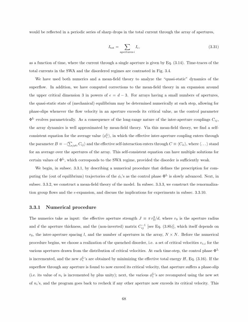
would be reflected in a periodic series of sharp drops in the total current through the array of apertures,

Itot =∑

apertures i

Ii, (3.31)

as a function of time, where the current through a single aperture is given by Eq. (3.14). Time-traces of the

total currents in the SWA and the disordered regimes are contrasted in Fig. 3.4.

We have used both numerics and a mean-field theory to analyze the “quasi-static” dynamics of the

superflow. In addition, we have computed corrections to the mean-field theory in an expansion around

the upper critical dimension 3 in powers of ε = d − 3. For arrays having a small numbers of apertures,

the quasi-static state of (mechanical) equilibrium may be determined numerically at each step, allowing for

phase-slips whenever the flow velocity in an aperture exceeds its critical value, as the control parameter

ΦL evolves parametrically. As a consequence of the long-range nature of the inter-aperture couplings Cij ,

the array dynamics is well approximated by mean-field theory. Via this mean-field theory, we find a self-

consistent equation for the average value 〈φLi 〉, in which the effective inter-aperture coupling enters through

the parameterB ≡ −〈∑j 6=i Cij〉 and the effective self-interaction enters through C ≡ 〈Cii〉, where 〈. . . 〉 stand

for an average over the apertures of the array. This self-consistent equation can have multiple solutions for

certain values of ΦL, which corresponds to the SWA regime, provided the disorder is sufficiently weak.

We begin, in subsec. 3.3.1, by describing a numerical procedure that defines the prescription for com-

puting the (out of equilibrium) trajectories of the φi’s as the control phase ΦL is slowly advanced. Next, in

subsec. 3.3.2, we construct a mean-field theory of the model. In subsec. 3.3.3, we construct the renormaliza-

tion group flows and the ε-expansion, and discuss the implications for experiments in subsec. 3.3.10.

3.3.1 Numerical procedure

The numerics take as input: the effective aperture strength J ≡ π r20/d, where r0 is the aperture radius

and d the aperture thickness, and the (non-inverted) matrix C−1ij [see Eq. (3.8b)], which itself depends on

r0, the inter-aperture spacing l, and the number of apertures in the array, N × N . Before the numerical

procedure begins, we choose a realization of the quenched disorder, i.e. a set of critical velocities vc,i for the

various apertures drawn from the distribution of critical velocities. At each time-step, the control phase ΦL

is incremented, and the new φLi ’s are obtained by minimizing the effective total energy H , Eq. (3.16). If the

superflow through any aperture is found to now exceed its critical velocity, that aperture suffers a phase-slip

(i.e. its value of ni is incremented by plus unity); next, the various φLi ’s are recomputed using the new set

of ni’s, and the program goes back to recheck if any other aperture now exceeds its critical velocity. This

68

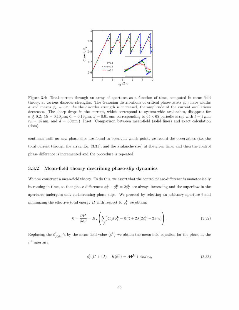
3 4 5 6 7 8 9

0.6

0.7

0.8

0.9

1

ωJ t/2 π

Cur

rent

, I/I c

σ=0.1

σ=0.3

σ=0.5

Figure 3.4: Total current through an array of apertures as a function of time, computed in mean-fieldtheory, at various disorder strengths. The Gaussian distributions of critical phase-twists φc,i have widthsσ and means φc = 3π. As the disorder strength is increased, the amplitude of the current oscillationsdecreases. The sharp drops in the current, which correspond to system-wide avalanches, disappear forσ & 0.2. (B = 0.10µm; C = 0.19µm; J = 0.01µm; corresponding to 65× 65 periodic array with ` = 3µm,r0 = 15 nm, and d = 50 nm.) Inset: Comparison between mean-field (solid lines) and exact calculation(dots).

continues until no new phase-slips are found to occur, at which point, we record the observables (i.e. the

total current through the array, Eq. (3.31), and the avalanche size) at the given time, and then the control

phase difference is incremented and the procedure is repeated.

3.3.2 Mean-field theory describing phase-slip dynamics

We now construct a mean-field theory. To do this, we assert that the control phase-difference is monotonically

increasing in time, so that phase differences φLi − φR

i = 2φLi are always increasing and the superflow in the

apertures undergoes only ni-increasing phase slips. We proceed by selecting an arbitrary aperture i and

minimizing the effective total energy H with respect to φLi we obtain:

0 =∂H

∂φLi

= Ks

∑

j

Cij(φLj − ΦL) + 2J(2φL

i − 2πni)

. (3.32)

Replacing the φLj(6=i)’s by the mean-field value 〈φL〉 we obtain the mean-field equation for the phase at the

ith aperture:

φLi (C + 4J)−B〈φL〉 = AΦL + 4πJ ni, (3.33)

69

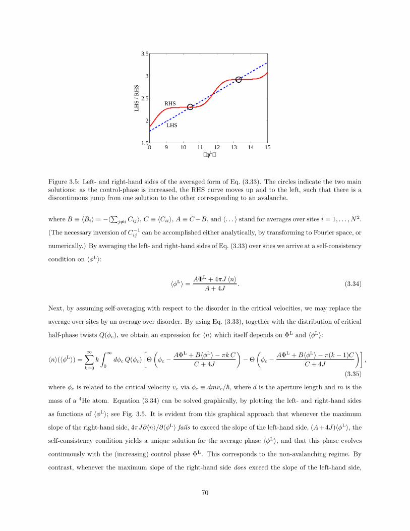
8 9 10 11 12 13 14 151.5

2

2.5

3

3.5

⟨ φL⟩

LH

S / R

HS

LHS

RHS

Figure 3.5: Left- and right-hand sides of the averaged form of Eq. (3.33). The circles indicate the two mainsolutions: as the control-phase is increased, the RHS curve moves up and to the left, such that there is adiscontinuous jump from one solution to the other corresponding to an avalanche.

where B ≡ 〈Bi〉 = −〈∑j 6=i Cij〉, C ≡ 〈Cii〉, A ≡ C−B, and 〈. . . 〉 stand for averages over sites i = 1, . . . , N 2.

(The necessary inversion of C−1ij can be accomplished either analytically, by transforming to Fourier space, or

numerically.) By averaging the left- and right-hand sides of Eq. (3.33) over sites we arrive at a self-consistency

condition on 〈φL〉:

〈φL〉 =AΦL + 4πJ 〈n〉

A+ 4J. (3.34)

Next, by assuming self-averaging with respect to the disorder in the critical velocities, we may replace the

average over sites by an average over disorder. By using Eq. (3.33), together with the distribution of critical

half-phase twists Q(φc), we obtain an expression for 〈n〉 which itself depends on ΦL and 〈φL〉:

〈n〉(〈φL〉) =

∞∑

k=0

k

∫ ∞

0

dφc Q(φc)

[Θ

(φc −

AΦL +B〈φL〉 − πk CC + 4J

)−Θ

(φc −

AΦL +B〈φL〉 − π(k − 1)C

C + 4J

)],

(3.35)

where φc is related to the critical velocity vc via φc ≡ dmvc/~, where d is the aperture length and m is the

mass of a 4He atom. Equation (3.34) can be solved graphically, by plotting the left- and right-hand sides

as functions of 〈φL〉; see Fig. 3.5. It is evident from this graphical approach that whenever the maximum

slope of the right-hand side, 4πJ∂〈n〉/∂〈φL〉 fails to exceed the slope of the left-hand side, (A+4J)〈φL〉, the

self-consistency condition yields a unique solution for the average phase 〈φL〉, and that this phase evolves

continuously with the (increasing) control phase ΦL. This corresponds to the non-avalanching regime. By

contrast, whenever the maximum slope of the right-hand side does exceed the slope of the left-hand side,

70

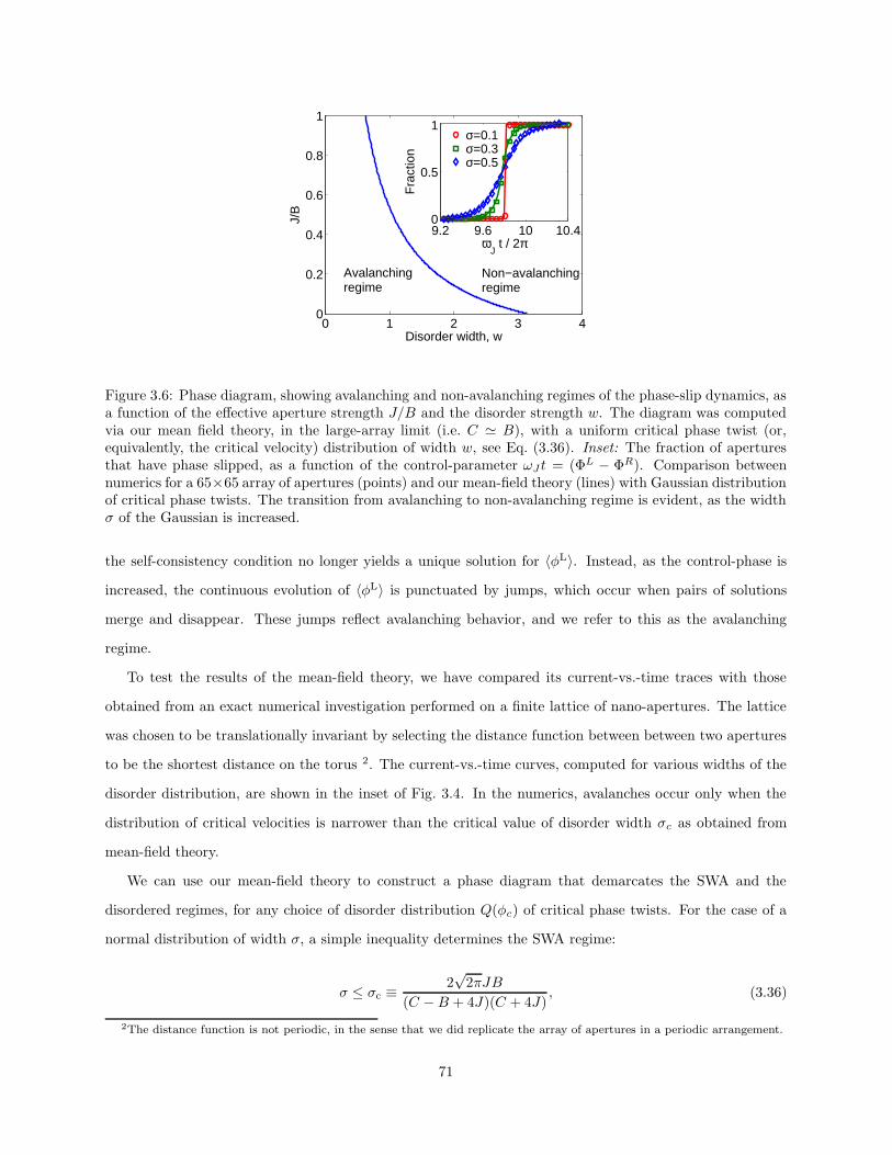
0 1 2 3 40

0.2

0.4

0.6

0.8

1

Disorder width, w

J/B

9.2 9.6 10 10.40

0.5

1

ωJ t / 2π

Fra

ctio

n

σ=0.1σ=0.3σ=0.5

Avalanchingregime

Non−avalanchingregime

Figure 3.6: Phase diagram, showing avalanching and non-avalanching regimes of the phase-slip dynamics, asa function of the effective aperture strength J/B and the disorder strength w. The diagram was computedvia our mean field theory, in the large-array limit (i.e. C ' B), with a uniform critical phase twist (or,equivalently, the critical velocity) distribution of width w, see Eq. (3.36). Inset: The fraction of aperturesthat have phase slipped, as a function of the control-parameter ωJ t = (ΦL − ΦR). Comparison betweennumerics for a 65×65 array of apertures (points) and our mean-field theory (lines) with Gaussian distributionof critical phase twists. The transition from avalanching to non-avalanching regime is evident, as the widthσ of the Gaussian is increased.

the self-consistency condition no longer yields a unique solution for 〈φL〉. Instead, as the control-phase is

increased, the continuous evolution of 〈φL〉 is punctuated by jumps, which occur when pairs of solutions

merge and disappear. These jumps reflect avalanching behavior, and we refer to this as the avalanching

regime.

To test the results of the mean-field theory, we have compared its current-vs.-time traces with those

obtained from an exact numerical investigation performed on a finite lattice of nano-apertures. The lattice

was chosen to be translationally invariant by selecting the distance function between between two apertures

to be the shortest distance on the torus 2. The current-vs.-time curves, computed for various widths of the

disorder distribution, are shown in the inset of Fig. 3.4. In the numerics, avalanches occur only when the

distribution of critical velocities is narrower than the critical value of disorder width σc as obtained from

mean-field theory.

We can use our mean-field theory to construct a phase diagram that demarcates the SWA and the

disordered regimes, for any choice of disorder distribution Q(φc) of critical phase twists. For the case of a

normal distribution of width σ, a simple inequality determines the SWA regime:

σ ≤ σc ≡2√

2πJB

(C −B + 4J)(C + 4J), (3.36)

2The distance function is not periodic, in the sense that we did replicate the array of apertures in a periodic arrangement.

71

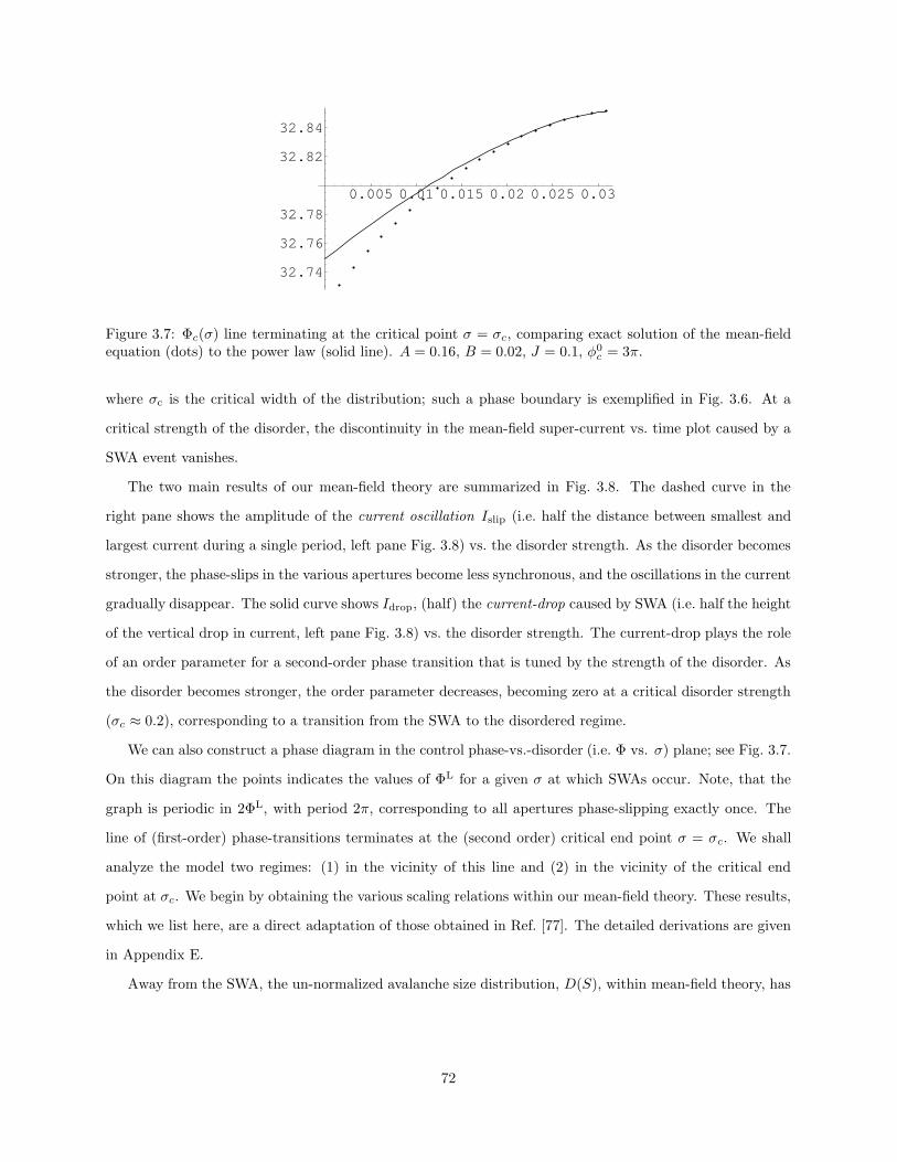
0.005 0.01 0.015 0.02 0.025 0.03

32.74

32.76

32.78

32.82

32.84

Figure 3.7: Φc(σ) line terminating at the critical point σ = σc, comparing exact solution of the mean-fieldequation (dots) to the power law (solid line). A = 0.16, B = 0.02, J = 0.1, φ0

c = 3π.

where σc is the critical width of the distribution; such a phase boundary is exemplified in Fig. 3.6. At a

critical strength of the disorder, the discontinuity in the mean-field super-current vs. time plot caused by a

SWA event vanishes.

The two main results of our mean-field theory are summarized in Fig. 3.8. The dashed curve in the

right pane shows the amplitude of the current oscillation Islip (i.e. half the distance between smallest and

largest current during a single period, left pane Fig. 3.8) vs. the disorder strength. As the disorder becomes

stronger, the phase-slips in the various apertures become less synchronous, and the oscillations in the current

gradually disappear. The solid curve shows Idrop, (half) the current-drop caused by SWA (i.e. half the height

of the vertical drop in current, left pane Fig. 3.8) vs. the disorder strength. The current-drop plays the role

of an order parameter for a second-order phase transition that is tuned by the strength of the disorder. As

the disorder becomes stronger, the order parameter decreases, becoming zero at a critical disorder strength

(σc ≈ 0.2), corresponding to a transition from the SWA to the disordered regime.

We can also construct a phase diagram in the control phase-vs.-disorder (i.e. Φ vs. σ) plane; see Fig. 3.7.

On this diagram the points indicates the values of ΦL for a given σ at which SWAs occur. Note, that the

graph is periodic in 2ΦL, with period 2π, corresponding to all apertures phase-slipping exactly once. The

line of (first-order) phase-transitions terminates at the (second order) critical end point σ = σc. We shall

analyze the model two regimes: (1) in the vicinity of this line and (2) in the vicinity of the critical end

point at σc. We begin by obtaining the various scaling relations within our mean-field theory. These results,

which we list here, are a direct adaptation of those obtained in Ref. [77]. The detailed derivations are given

in Appendix E.

Away from the SWA, the un-normalized avalanche size distribution, D(S), within mean-field theory, has

72

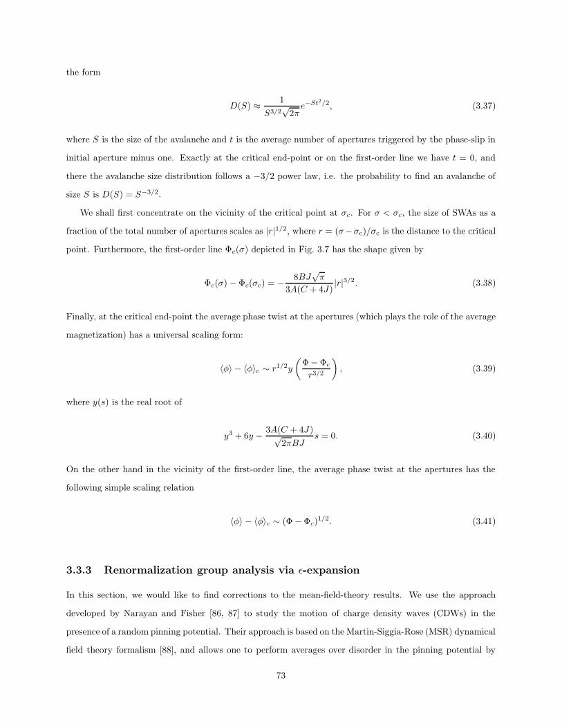
the form

D(S) ≈ 1

S3/2√

2πe−St2/2, (3.37)

where S is the size of the avalanche and t is the average number of apertures triggered by the phase-slip in

initial aperture minus one. Exactly at the critical end-point or on the first-order line we have t = 0, and

there the avalanche size distribution follows a −3/2 power law, i.e. the probability to find an avalanche of

size S is D(S) = S−3/2.

We shall first concentrate on the vicinity of the critical point at σc. For σ < σc, the size of SWAs as a

fraction of the total number of apertures scales as |r|1/2, where r = (σ−σc)/σc is the distance to the critical

point. Furthermore, the first-order line Φc(σ) depicted in Fig. 3.7 has the shape given by

Φc(σ) − Φc(σc) = − 8BJ√π

3A(C + 4J)|r|3/2. (3.38)

Finally, at the critical end-point the average phase twist at the apertures (which plays the role of the average

magnetization) has a universal scaling form:

〈φ〉 − 〈φ〉c ∼ r1/2y

(Φ− Φc

r3/2

), (3.39)

where y(s) is the real root of

y3 + 6y − 3A(C + 4J)√2πBJ

s = 0. (3.40)

On the other hand in the vicinity of the first-order line, the average phase twist at the apertures has the

following simple scaling relation

〈φ〉 − 〈φ〉c ∼ (Φ− Φc)1/2. (3.41)

3.3.3 Renormalization group analysis via ε-expansion

In this section, we would like to find corrections to the mean-field-theory results. We use the approach

developed by Narayan and Fisher [86, 87] to study the motion of charge density waves (CDWs) in the

presence of a random pinning potential. Their approach is based on the Martin-Siggia-Rose (MSR) dynamical

field theory formalism [88], and allows one to perform averages over disorder in the pinning potential by

73

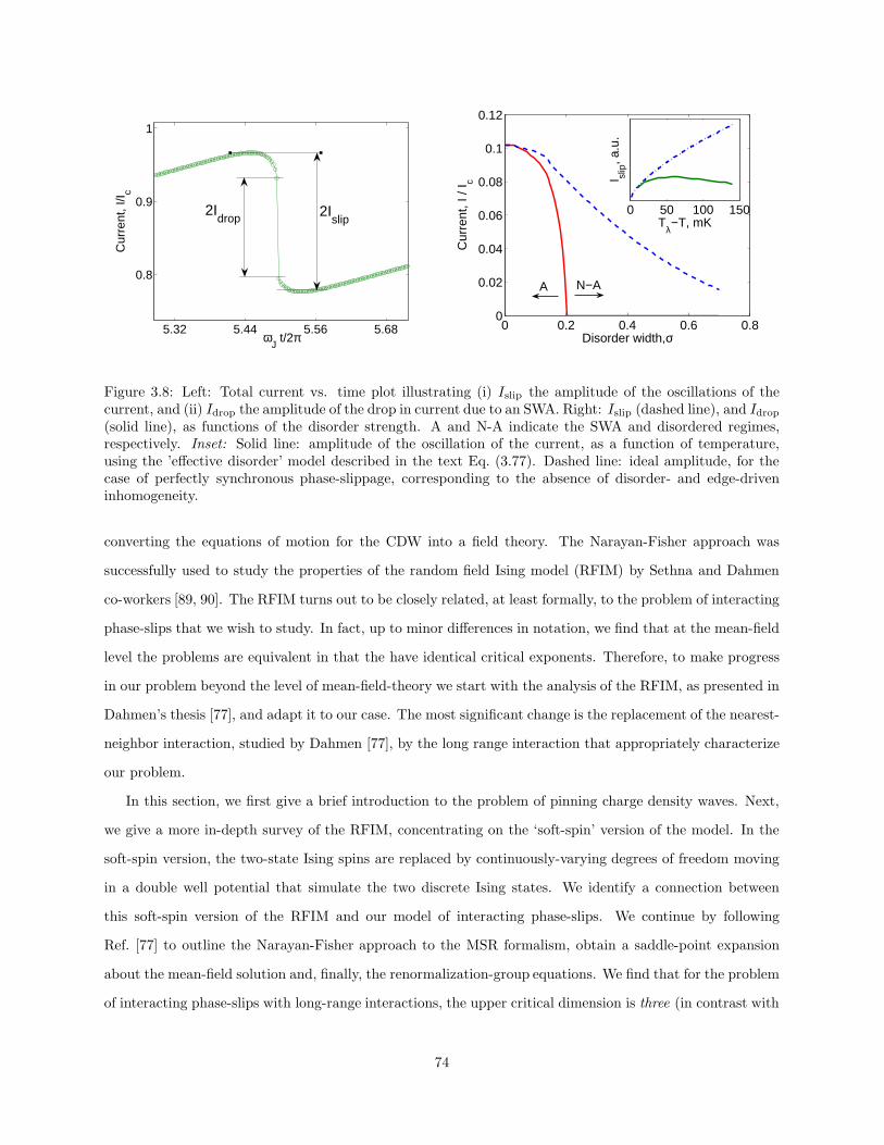
5.32 5.44 5.56 5.68

0.8

1

0.9

ωJ t/2π

Cur

rent

, I/I c

2Idrop 2I

slip

0 0.2 0.4 0.6 0.80

0.02

0.04

0.06

0.08

0.1

0.12

Disorder width,σ

Cur

rent

, I /

I c

0 50 100 150T

λ−T, mK

I slip

, a.u

.

N−AA

Figure 3.8: Left: Total current vs. time plot illustrating (i) Islip the amplitude of the oscillations of thecurrent, and (ii) Idrop the amplitude of the drop in current due to an SWA. Right: Islip (dashed line), and Idrop

(solid line), as functions of the disorder strength. A and N-A indicate the SWA and disordered regimes,respectively. Inset: Solid line: amplitude of the oscillation of the current, as a function of temperature,using the ’effective disorder’ model described in the text Eq. (3.77). Dashed line: ideal amplitude, for thecase of perfectly synchronous phase-slippage, corresponding to the absence of disorder- and edge-driveninhomogeneity.

converting the equations of motion for the CDW into a field theory. The Narayan-Fisher approach was

successfully used to study the properties of the random field Ising model (RFIM) by Sethna and Dahmen

co-workers [89, 90]. The RFIM turns out to be closely related, at least formally, to the problem of interacting

phase-slips that we wish to study. In fact, up to minor differences in notation, we find that at the mean-field

level the problems are equivalent in that the have identical critical exponents. Therefore, to make progress

in our problem beyond the level of mean-field-theory we start with the analysis of the RFIM, as presented in

Dahmen’s thesis [77], and adapt it to our case. The most significant change is the replacement of the nearest-

neighbor interaction, studied by Dahmen [77], by the long range interaction that appropriately characterize

our problem.

In this section, we first give a brief introduction to the problem of pinning charge density waves. Next,

we give a more in-depth survey of the RFIM, concentrating on the ‘soft-spin’ version of the model. In the

soft-spin version, the two-state Ising spins are replaced by continuously-varying degrees of freedom moving

in a double well potential that simulate the two discrete Ising states. We identify a connection between

this soft-spin version of the RFIM and our model of interacting phase-slips. We continue by following

Ref. [77] to outline the Narayan-Fisher approach to the MSR formalism, obtain a saddle-point expansion

about the mean-field solution and, finally, the renormalization-group equations. We find that for the problem

of interacting phase-slips with long-range interactions, the upper critical dimension is three (in contrast with

74

the value of six for the nearest-neighbor case considered for the RFIM). Next, we identify the various fixed

points and obtain the corresponding critical exponents.

3.3.4 Pinning of charge density waves

In many, especially lower-dimensional, systems, due the interaction between electrons and phonons, the

discrete lattice translational invariance may be spontaneously broken giving rise to a CDW, i.e., a periodic

modulation of the electron density accompanied by lattice deformations. This mechanism is known as the

Pierel’s instability. In some CDW systems the modulation of the electron density is commensurate with the

underlying lattice, which typically leads to the locking of the modulation to the lattice. Others, however,

are incommensurate with the underlying lattice and thus, in principle, are energetically free to slide through

the lattice. Narayan-Fisher concentrate on the incommensurate CDWs, and study the pinning of this sliding

motion by impurities within the lattice. They describe the CDW by a collection of phases of the periodic

lattice distortion associated with the CDW specified at the sites of a lattice φi. The dynamics of these

phases are modeled via the equation of motion

∂φj

∂t= − ∂H

∂φj=∑

i

Jij(φi − φj)− dVj

dφj+ F, (3.42)

where Jij describes the interaction between phases at site i and j (that are generally taken to be nearest-

neighbor), Vj is the random pinning potential for the jth site (for the case of CDWs, Vj is a random but

periodic in φj potential, having a random amplitude and phase-shift on the various sites of the lattice), and

F is a driving force (due, e.g., to an external electric field) that pushes the CDW forward (i.e. to higher

values of φi). When the externally-applied force is sufficiently large, the CDW suffers the so-called de-

pinning transition and starts sliding. The form of the equation of motion describing CDWs is very general

and, in fact, can also be used to describe both the soft-spin version of the RFIM and the present problem of

interacting phase-slips. The main differences between the three problems arise from the form and range of

the interaction Jij and the form of the pinning potential Vj .

3.3.5 Soft-spin random field Ising model

The RFIM is a model designed to capture the essential properties of realistic magnets, in particular how

the magnetization changes, in a history dependent way, as the externally-applied magnetic field is varied.

Like the standard Ising model, the RFIM is composed of interacting spins in an external magnetic field.

Each spin j has a magnetic moment sj that can be in one of two states, sj = ±1, and the interaction is

75

assumed to be nearest-neighbor and ferromagnetic (i.e. favoring alignment of spins i and j). In addition to

the externally-applied magnetic field F , associated with each domain is a local random field fi.

Unlike the standard Ising model, in this context we treat the RFIM not as a thermodynamic model but

instead as a non-linear dynamics model. Therefore, instead of weighting states using Boltzmann factors,

we look at the dynamics of the spins. The dynamics are described by the following rules: One imagines

beginning with an external field F so large that all the Ising spins are aligned with it. Next, one imagines

slowly change F , and whenever the local field Fj , where

Fj = F +∑

i(6=j)

Jijsj + fj , (3.43)

acting on a particular Ising spin sj , changes sign, the Ising spin flips so as to remain aligned with the

local field. When a spin flips, the neighbors of the spin that has flipped encounter a change in their local

field Fi. This change in the local field of the neighboring spins can induce one or more of them to flip. If

the distribution of the random fields fi is sufficiently narrow, the initial spin flip may launch a cascade of

secondary spin-flips, and this is called an avalanche.

The dynamics of the RFIM cannot be (easily) written in the form of Eq. (3.42) due to the discrete nature

of the Ising spins. Therefore, it is convenient to study the soft-spin version of the RFIM, in which the Ising

spins Sj are replaced by the continuous variables φj . The φj ’s are subject to move in the potentials

Vj =

k/2(φj + 1)2 − φjfj ; for φi < 0,

k/2(φj − 1)2 − φjfj ; for φi > 0,(3.44)

where, as before, fj is the random local field. This form of the potential serves two purposes: (1) its two

minima simulate the two Ising states, and (2) it captures the effect of the random local field fj by shifting

the relative energy of the two minima. The dynamics of these soft-spins are described by the equation of

motion Eq. (3.42), with Vj specified by Eq. (3.44), and Jij = 1/z if i and j are nearest neighbors and Jij = 0

otherwise, where z is the coordination number of the lattice (e.g. six for a three-dimensional square lattice).

3.3.6 Connection between the random field Ising model and the present

model of interacting phase-slips

We begin by considering an equation of motion that would capture the properties of the model of interacting

phase-slips. That is, we would like to identify an equation of motion for the phases across the apertures that

would reproduce the trajectories that we obtain when the system follows the rules described in subsec. 3.3.1.

76

In the limit of an adiabatically-slowly varying control-phase Φ, the solution of the equation of motion

∂φj

∂t= − ∂H

∂φj, (3.45)

where H is the total energy that appears in Eq. (3.16), will, indeed, trace out trajectories identical to those

obtained by the rules described in subsec. 3.3.1.

To make a connection with the RFIM, we write down the equation of motion explicitly for the problem

of interacting phase-slips:

∂φj

∂t=∑

i(6=j)

Cijφi + Φ∑

j

Cij − J(φj − π

∞∑

k=0

θ(φj − φc,j − πk)

), (3.46)

where θ(·) is the unit step function, and φc,i is the random, aperture-specific, critical phase-twist, and,

crucially, we continue working under the assumption that all the apertures have phase slipped either n or

n+ 1 times3. Next, we compare this equation of motion to the one obtained for the RFIM:

∂sj

∂t= −2

∑

i(6=j)

Jijsi + fj + F − ksj + 2k

(θ(sj)− 1

2

). (3.47)

The identification between the two equations of motion is made explicit via the following transformations:

Cij = −2Jij , (3.48)

Φ∑

j

Cij = F, (3.49)

sj = φj − φc,j (3.50)

φc,j = (2Jij + kδij)−1fi. (3.51)

With these transformations, we map the problem of interacting phase-slips on to a version of the RFIM, the

only difference being the substitution of long- for short-range interactions.

Having made this identification, we proceed by developing the MSR formalism for a generic equation of

motion, and make the restriction to this specific form only when it becomes necessary for the computation

of the coefficients in the expansion about the saddle-point.

3We have ignored the (inconsequential) δ functions that arise when taking the derivative of the θ functions in the piningpotential.

77

3.3.7 Martin-Siggia-Rose formalism

The basic idea is to convert the description of dynamics based on the equation of motion, Eq. (3.42), into a

description involving an integral over histories. This is accomplished via the MSR formalism, which provides

a way to write a path integral that, for a given initial conditions and disorder, selects only the single path

that obeys the equation of motion. Consider introducing the partition function Z via

1 = Z =

∫[dφ][dφ]J [φ] exp

i∑

i

∫dt φi

(∂φi

∂t+∂H

∂φi

], (3.52)

where J [φ] is a functional Jacobian determinant that ensures that the partition function is indeed unity by

guaranteeing that all of the δ-functions integrate to unity. The form of J [φ] depends on the definition of

the path integral, in the sense of discretization in time, and we shall adopt the one for which the correct

value is J [φ] ≡ 1. Upon performing the path-integral over φ, we obtain a δ-function that selects only that

path that satisfies the equation of motion. One advantage of the MSR formalism is that one does not have

to deal with a random denominator when computing observables; this is because Z ≡ 1, independent of the

randomness.

3.3.8 Saddle-point expansion

Narayan and Fisher continue by introducing the disorder-averaged partition function Z:

1 = Z =

∫[dφ][dφ]

⟨exp

[i∑

i

∫dt φi

(∂φi

∂t+∂H

∂φi

)]⟩(3.53)

where 〈· · · 〉 stands for the disorder average. Next, following Sompolinsky and Zippelius [91], Narayan and

Fisher introduce the conjugate fields Φ and Φ. The goal of this transformation is to separate the disorder

average and the inter-site interaction through the introduction of an axillary field, which allows us to carry

out the disorder averages on different sites independently. Upon the introduction of the conjugate fields, the

disorder-averaged partition function becomes

Z =

∫[dΦ][dΦ]

∏

j

Zj [Φj , Φj ] exp

−∫dt ΦiJ

−1ijΦj

, (3.54)

where Zj [Φj , Φj ] is a path integral over the fields φj and φj on a single site only

Zj [Φj , Φj ] =

∫[dφ][dφ]

⟨exp

∫dt

[Φjφj + iφj

(∂tφj − Φj + φj +

∂H

∂φj

)]⟩, (3.55)

78

and H is the energy without the Jij term. If we were to integrate over the conjugate fields, Φ and Φ, we

would recover the original partition function, Eq. (3.53). The introduction of the conjugate fields allows us to

perform a perturbative expansion not about the trivial point (Φ = Φ = 0), but rather about the mean-field

solution, which corresponds to the saddle-point of the action in Eq. (3.54). To find this saddle-point, we

vary this action with respect to Φj and Φj , thus obtaining the following equations for the location (Φ0j and

Φ0j ) of the saddle point:

−J−1ij Φ0

i − i〈φj〉l,Φ0,Φ0 = 0, (3.56)

−J−1ij Φ0

i + 〈φi〉l,Φ0,Φ0 = 0, (3.57)

where 〈. . . 〉l stands for the local (i.e. single-site) average over the disorder, computed with η and η fixed at

their mean-field values, that is

〈φj〉l,Φ0,Φ0 = i∂Zj [Φj , Φj ]

∂Φj

∣∣∣∣∣Φ0,Φ0

, (3.58)

〈φj〉l,Φ0,Φ0 =∂Zj [Φj , Φj ]

∂Φj

∣∣∣∣∣Φ0,Φ0

. (3.59)

(3.60)

By solving Eqs. (3.56, 3.57) we obtain the self-consistent form

Φ0j = 0, (3.61)

Φ0j = M(t) = 〈φj〉l,Φ0,Φ0 , (3.62)

where M(t) is the disorder-averaged solution of the mean-field equation of motion

∂tφj = M(t)− ∂H

∂φj. (3.63)

We are now in a position to perform an expansion about the saddle point. We begin by introducing the

(shifted) variables ηj and ηj , which measure the deviation from the saddle point solution:

ηj ≡ Φj − Φ0j , ηj ≡ Φj − Φ0

j . (3.64)

79

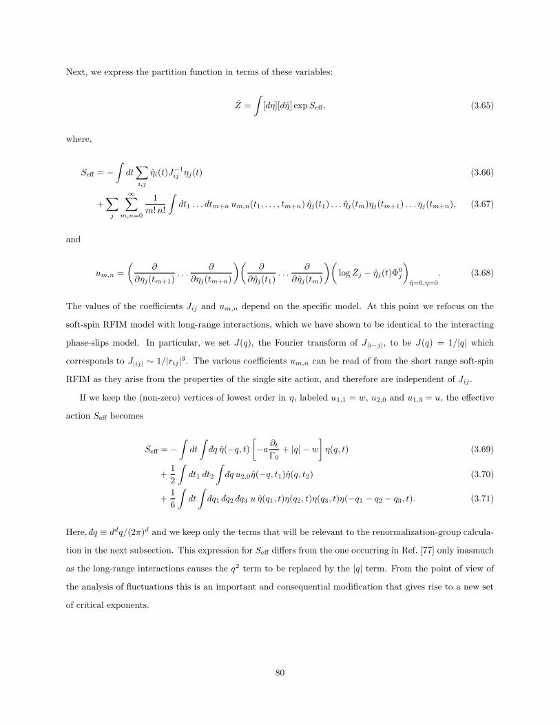
Next, we express the partition function in terms of these variables:

Z =

∫[dη][dη] expSeff, (3.65)

where,

Seff = −∫dt∑

i,j

ηi(t)J−1ij ηj(t) (3.66)

+∑

j

∞∑

m,n=0

1

m!n!

∫dt1 . . . dtm+n um,n(t1, . . . , tm+n) ηj(t1) . . . ηj(tm)ηj(tm+1) . . . ηj(tm+n), (3.67)

and

um,n =

(∂

∂ηj(tm+1). . .

∂

∂ηj(tm+n)

)(∂

∂ηj(t1). . .

∂

∂ηj(tm)

)(log Zj − ηj(t)Φ0

j

)

η=0,η=0

. (3.68)

The values of the coefficients Jij and um,n depend on the specific model. At this point we refocus on the

soft-spin RFIM model with long-range interactions, which we have shown to be identical to the interacting

phase-slips model. In particular, we set J(q), the Fourier transform of J|i−j|, to be J(q) = 1/|q| which

corresponds to J|ij| ∼ 1/|rij |3. The various coefficients um,n can be read of from the short range soft-spin

RFIM as they arise from the properties of the single site action, and therefore are independent of Jij .

If we keep the (non-zero) vertices of lowest order in η, labeled u1,1 = w, u2,0 and u1,3 = u, the effective

action Seff becomes

Seff = −∫dt

∫dq η(−q, t)

[−a ∂t

Γ0+ |q| − w

]η(q, t) (3.69)

+1

2

∫dt1 dt2

∫dq u2,0η(−q, t1)η(q, t2) (3.70)

+1

6

∫dt

∫dq1 dq2 dq3 u η(q1, t)η(q2, t)η(q3, t)η(−q1 − q2 − q3, t). (3.71)

Here, dq ≡ ddq/(2π)d and we keep only the terms that will be relevant to the renormalization-group calcula-

tion in the next subsection. This expression for Seff differs from the one occurring in Ref. [77] only inasmuch

as the long-range interactions causes the q2 term to be replaced by the |q| term. From the point of view of

the analysis of fluctuations this is an important and consequential modification that gives rise to a new set

of critical exponents.

80

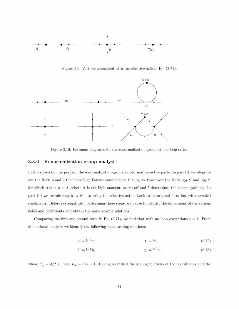
η η u2,0u

Figure 3.9: Vertices associated with the effective action, Eq. (3.71).

= +

u

u2,0

= +

uu

u2,0

Figure 3.10: Feynman diagrams for the renormalization group at one loop order.

3.3.9 Renormalization-group analysis

In this subsection we perform the renormalization-group transformation in two parts: In part (i) we integrate

out the fields η and η that have high Fourier components; that is, we trace over the fields η(q, t) and η(q, t)

for which Λ/b < q < Λ, where Λ is the high-momentum cut-off and b determines the coarse graining. In

part (ii) we rescale length by b−1 to bring the effective action back to its original form but with rescaled

coefficients. Before systematically performing these steps, we pause to identify the dimensions of the various

fields and coefficients and obtain the naive scaling relations.

Comparing the first and second term in Eq. (3.71), we find that with no loop corrections z = 1. From

dimensional analysis we identify the following naive scaling relations:

q′ = b−1q, t′ = bt, (3.72)

η′ = bCpη, η′ = bCpη, (3.73)

where Cp = d/2 + 1 and Cp = d/2 − 1. Having identified the scaling relations of the coordinates and the

81

fields, we can compute the naive scaling relation for an arbitrary vertex:

u′m,n = b(2−(m+n))d/2+num,n. (3.74)

From this relation, we see that for d > 4 all super-quadratic vertices are irrelevant. Below four dimensions,

the first vertex to become relevant is u1,2. However, at the critical end-point, σ = σc, that we are interested

in u1,2 ≡ 0. Therefore, we must look at the next most relevant non-zero vertex u1,3. From Eq. (3.74), we

see that u1,3 is relevant in less than three dimensions.

Next, we perform the renormalization-group transformation and find the scaling relations to one-loop

order. The diagrams involved in tracing out the high momentum modes to this order are shown in Fig. 3.10.

At this order, u2,0 is found to be fixed, while both w and u are found to flow at both the tree-level and with

one-loop corrections (see Fig. 3.10). The details of this calculations closely follow Chapter 7 of Ref. [77] and

are provided in Appendix F. The resulting flow equations are

v′ = v + v log(b)

(ε+

3v

2π2

), (3.75)

w′ = b

(w +

v

2

1

2π2

[Λ

(1− 1

b

)+ 2w log b

]), (3.76)

where v = uu1,2. As described in Appendix F, these flow equations have two fixed points, the Gaussian

fixed point located at v = 0 and u = 0 and the Wilson-Fisher fixed point v = − 2π2

3 ε and w = εΛ6

11−ε/3 .

The properties of the system near criticality, in particular the critical exponents, may be obtained from

the analysis of the linearized flow equations in the vicinity of the fixed points, see Appendix F. For d > 3, the

Gaussian fixed point has one stable and one unstable eigendirection while the Wilson-Fisher fixed point has

two unstable eigendirections. Therefore the Gaussian fixed point controls the flows, and we can read off the

correlation length critical exponent ν from the unstable eigenvalue of the Gaussian fixed point ν = 1/yt = 1.

On the other hand for d < 3, the situation is reversed and the Gaussian fixed point has two unstable

eigendirections, while the Wilson-Fisher fixed point has one stable and one unstable eigendirection, and the

correlation length critical exponent becomes ν = 1/yt = 1 + ε/3.

3.3.10 Implications for experiment

In their experiments [65], the Berkeley group measured the amplitude of the “whistle” (i.e. the amplitude

of the current oscillations Islip) as a function of temperature at a fixed chemical potential difference. These

experiments found an onset of current oscillations at Tλ. As the temperature was lowered below Tλ, Islip

82

begins by increasing from zero, and then decreases gradually. To obtain the temperature dependence of Islip,

we consider the origin of the disorder in the critical velocities, which we have until now been treating as a

completely phenomenological parameter. Thus, we extend the model for the critical velocity, Eq. (3.15), to

include the effect of disorder by hypothesizing that

vc,i(T ) ' ~

mξ(T )

(1 +

xi

r0

), (3.77)

where xi is a single, temperature-independent length, characterizing surface roughness in the ith aperture,

and we take it to have a Gaussian distribution. For Tλ−T > 10 mK, we can compare the results of our model

to those of the experiments. The general features are reproduced: the initial increase in Islip is associated

with an increase in the superfluid fraction; the gradual decrease at lower temperatures is due to the loss of

synchronicity amongst the apertures, which is caused by the effective increase in the strength of the disorder.

To demonstrate these features, we plot the amplitude of the current oscillations vs. temperature; see the

inset in Fig. 3.8, for which we have used a Gaussian distribution of xi’s of standard deviation σx = 0.6 nm.

We also note that the general features of the current-vs.-time traces, Fig. 3.4, are similar to those of

the Type III experiments described in Ref. [65]. In both, as the temperature is lowered (i.e. the disorder is

increased), the avalanche gradually disappears, and then so do the oscillations in the current.

Thermal fluctuations

Thermal fluctuations of the phases can wash out the disorder-driven phase transition if they exceed the

width of the disorder distribution, and if they are sufficiently strong they can also wash out the “whistle.”

The main mechanism by which thermal fluctuations act is by causing random premature phase slips before

the critical velocity is reached. Thus, the thermal fluctuations effectively broaden the width of the critical

velocity distribution. As suggested by Sato [92], we can model this effect by a stochastic approach in which we

choose a new critical velocity for an aperture that has just phase slipped from a distribution specific to that

aperture, where the distribution describe both thermal effects and physical properties of the aperture. That

is for the ith aperture, the new critical velocity vc,i is chosen from a distribution centered on vc,i and with

width, the thermal width, common to all apertures. Within this approach, the effect of thermal fluctuations

is the same as choosing a new distribution of critical velocities for each cycle, and therefore within any cycle

thermal fluctuations act analogously to quenched disorder in the critical velocities. Moreover, if the two

sources of disorder are Gaussian, their effects can be combined into one “effective” source of width given by

(σ2q +σ2

t )1/2, where q and t correspond to quenched and thermal disorder. Therefore, as before, the criterion

for the avalanching regime can be estimated by Eq. (3.36), but now using the effective disorder width.

83

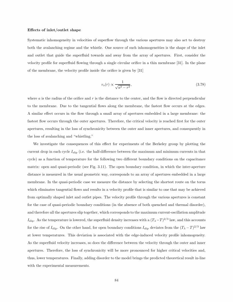
Effects of inlet/outlet shape

Systematic inhomogeneity in velocities of superflow through the various apertures may also act to destroy

both the avalanching regime and the whistle. One source of such inhomogeneities is the shape of the inlet

and outlet that guide the superfluid towards and away from the array of apertures. First, consider the

velocity profile for superfluid flowing through a single circular orifice in a thin membrane [31]. In the plane

of the membrane, the velocity profile inside the orifice is given by [31]

vs(r) ∝ 1√a2 − r2

, (3.78)

where a is the radius of the orifice and r is the distance to the center, and the flow is directed perpendicular

to the membrane. Due to the tangential flows along the membrane, the fastest flow occurs at the edges.

A similar effect occurs in the flow through a small array of apertures embedded in a large membrane: the

fastest flow occurs through the outer apertures. Therefore, the critical velocity is reached first for the outer

apertures, resulting in the loss of synchronicity between the outer and inner apertures, and consequently in

the loss of avalanching and “whistling.”

We investigate the consequences of this effect for experiments of the Berkeley group by plotting the

current drop in each cycle Islip (i.e. the half-difference between the maximum and minimum currents in that

cycle) as a function of temperature for the following two different boundary conditions on the capacitance

matrix: open and quasi-periodic (see Fig. 3.11). The open boundary condition, in which the inter-aperture

distance is measured in the usual geometric way, corresponds to an array of apertures embedded in a large

membrane. In the quasi-periodic case we measure the distance by selecting the shortest route on the torus

which eliminates tangential flows and results in a velocity profile that is similar to one that may be achieved

from optimally shaped inlet and outlet pipes. The velocity profile through the various apertures is constant

for the case of quasi-periodic boundary conditions (in the absence of both quenched and thermal disorder),

and therefore all the apertures slip together, which corresponds to the maximum current-oscillation amplitude

Islip. As the temperature is lowered, the superfluid density increases with a (Tλ−T )2/3 law, and this accounts

for the rise of Islip. On the other hand, for open boundary conditions Islip deviates from the (Tλ−T )2/3 law

at lower temperatures. This deviation is associated with the edge-induced velocity profile inhomogeneity.

As the superfluid velocity increases, so does the difference between the velocity through the outer and inner

apertures. Therefore, the loss of synchronicity will be more pronounced for higher critical velocities and,

thus, lower temperatures. Finally, adding disorder to the model brings the predicted theoretical result in-line

with the experimental measurements.

84

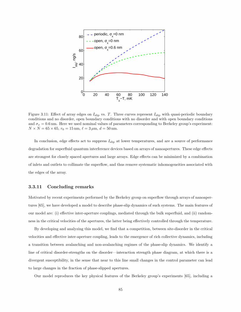
0 20 40 60 80 100 120 1400

20

40

60

80

Tλ−T, mK

I slip

, ng/

s

periodic, σx=0 nm

open, σx=0 nm

open, σx=0.6 nm

Figure 3.11: Effect of array edges on Islip vs. T . Three curves represent Islip with quasi-periodic boundaryconditions and no disorder, open boundary conditions with no disorder and with open boundary conditionsand σx = 0.6 nm. Here we used nominal values of parameters corresponding to Berkeley group’s experiment:N ×N = 65× 65, r0 = 15 nm, ` = 3µm, d = 50 nm.

In conclusion, edge effects act to suppress Islip at lower temperatures, and are a source of performance

degradation for superfluid quantum interference devices based on arrays of nanoapertures. These edge effects

are strongest for closely spaced apertures and large arrays. Edge effects can be minimized by a combination

of inlets and outlets to collimate the superflow, and thus remove systematic inhomogeneities associated with

the edges of the array.

3.3.11 Concluding remarks

Motivated by recent experiments performed by the Berkeley group on superflow through arrays of nanoaper-

tures [65], we have developed a model to describe phase-slip dynamics of such systems. The main features of

our model are: (i) effective inter-aperture couplings, mediated through the bulk superfluid, and (ii) random-

ness in the critical velocities of the apertures, the latter being effectively controlled through the temperature.

By developing and analyzing this model, we find that a competition, between site-disorder in the critical

velocities and effective inter-aperture coupling, leads to the emergence of rich collective dynamics, including

a transition between avalanching and non-avalanching regimes of the phase-slip dynamics. We identify a

line of critical disorder-strengths on the disorder—interaction strength phase diagram, at which there is a

divergent susceptibility, in the sense that near to this line small changes in the control parameter can lead

to large changes in the fraction of phase-slipped apertures.

Our model reproduces the key physical features of the Berkeley group’s experiments [65], including a

85

high-temperature synchronous regime, a low-temperature asynchronous regime, and a transition between

the two. We therefore feel that our model captures the essential physics explored in these experiments.

It is likely that technologically useful devices, such as ultra-precise gyrometers, can be designed to function

not only in the Josephson (i.e. reversible) regime but also in the phase-slippage (i.e. irreversible) regime,

provided that a large enough fraction of apertures can be arranged to slip sufficiently simultaneously so as to

produce a measurable “whistle” at the Josephson frequency [67]. We remark that, in the setting of multi-link

superconducting devices, it has been shown that the irreversible regime can be utilized for magnetic-field

and related phase-sensitive measurements [38].

86

Chapter 4

Conclusions

In this thesis we have explore superflows in multiply connected geometries. In particular we have concen-

trated on geometries with multiple constrictions and on interactions between phase-slips occurring in these

constrictions. We find and investigate many interesting physical phenomena in these systems, spanning from

non-linear physics and avalanches to superconducting-phase gradiometery.

87

Appendix A

Physical Scales

It is convenient to express the results of the long-wire model, Eqs. (2.41,2.45,2.46), in terms of macro-

scopic physical parameters. Following Tinkham and Lau [59], we express the condensation energy scale per

coherence length of wire as

E = 0.22 kBTc (1− t)3/2 Rq

RN

b

ξ(T = 0), (A.1)

where t ≡ T/Tc, RN is the normal-state resistance of the device, and Rq ≡ h/4e2 ≈ 6.5 kΩ is the quantum

of resistance. The LAMH prefactor for sequential phase slips then becomes

Ω =b√

1− tξ(T = 0)

(8√

2 E3 kBTc

)1/28kB(Tc − T )

π~, (A.2)

and for parallel phase slips it becomes

Ω =

(b√

1− tξ(T = 0)

)2(

16√

2E3 kBTc

)1/28kB(Tc − T )

π~. (A.3)

The remaining parameters in the model are RN , Tc and ξ(T = 0). The normal-state resistance and the

critical temperature may be obtained from the R vs. T curve. The coherence length may be obtained by

comparing E obtained from the critical current at low temperature, via

Ic =2

3√

3

16πEΦ0

, (A.4)

with E obtained via Eq. (A.1).

In experiments, it is expected that the two wires are not identical. The long-wire model can be easily

extended to this case. The number of parameters to be fitted would then expand to include the normal-state

resistance for each wire (only one of which is free, as the pair are constrained by the normal-state resistance

of the entire device, which can be extracted from the R vs. T curve), a zero-temperature coherence length

for each wire, and critical temperatures for each wire.

88

Appendix B

Ambegaokar-Halperin formula for

resistance of a damped

Josephson junction

In this appendix we reproduce the result of the Ambegaokar-Halperin Letter [5], but correcting typographical

errors. Eq. (9) of reference [5] should read

ν =V

IcR=

4π (eπγx − 1)

γ(∫ 2π

0 dθ∫ θ

0 dθ′ f(θ)

f(θ′) + eπγx∫ 2π

0 dθ∫ 2π

0 dθ′ f(θ)f(θ′)

) , (B.1)

where,

f(θ) = e12γ(xθ+cosθ), (B.2)

ν is related to the resistance of the shunted junction through R = νIcRN/I , x and γ are defined in Eq. 2.31b.

89

Appendix C

LA-MH theory for a single bridge

In this appendix we reproduce useful formulas from LA [6], and rewrite them in a way that is convenient for

further calculations, especially for numerical implementation. As in the case of single-wire LAMH theory,

one starts with the Ginzburg-Landau free energy

F =

∫ b/2

−b/2

(α|ψ|2 +

β

2|ψ|4 +

~2

2m|∇zψ|2

)dz. (C.1)

The relationships between the parameters of the Ginzburg-Landau free energy (α and β), the coherence

length ξ, the condensation energy per coherence length E , the critical field Hc, and the cross-sectional area

of the wire σ are given by α2

β =H2

c σ8π = E/ξ and ξ2 = ~

2

2m|α| . Following McCumber [30], it is convenient to

work in terms of the dimensionless units obtained using the transformations: |ψ|2 → αβ |ψ|2, z →

√2m|α|

~2 z,

and b→ b/ξ =√

2m|α|~2 b. In terms of these units, the free energy becomes

F = 2E∫ b/2

−b/2

(1

2(1− |ψ|2)2 + |∇zψ|2

)dz. (C.2)

The Ginzburg-Landau equation is obtained by varying the free energy:

δF = 0 ⇒ −ψ + |ψ|2ψ −∇2ψ = 0. (C.3)

By writing ψ = feiφ and taking the real and imaginary parts of the Ginzburg-Landau equation one obtains

−f + f3 + (φ′)2f = f ′′, (C.4)

2φ′f ′ + φ′′f = 0. (C.5)

From Eq. (C.5), one finds the current-conservation law:

f2φ′ = J, (C.6)

90

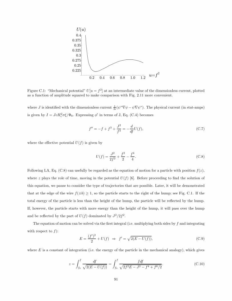
0.4

0.375

0.325

0.35

0.3

0.275

0.25

0.225

U(u)

u=f 20.2 0.4 0.6 0.8 1.0 1.2

Figure C.1: “Mechanical potential” U [u = f 2] at an intermediate value of the dimensionless current, plottedas a function of amplitude squared to make comparison with Fig. 2.11 more convenient.

where J is identified with the dimensionless current 12i (ψ

∗∇ψ−ψ∇ψ∗). The physical current (in stat-amps)

is given by I = JcH2cσξ/Φ0. Expressing φ′ in terms of J, Eq. (C.4) becomes

f ′′ = −f + f3 +J2

f3= − d

dfU(f), (C.7)

where the effective potential U(f) is given by

U(f) =J2

2f2+f2

2− f4

4. (C.8)

Following LA, Eq. (C.8) can usefully be regarded as the equation of motion for a particle with position f(z),

where z plays the role of time, moving in the potential U(f) [6]. Before proceeding to find the solution of

this equation, we pause to consider the type of trajectories that are possible. Later, it will be demonstrated

that at the edge of the wire f(±b) ≥ 1, so the particle starts to the right of the hump; see Fig. C.1. If the

total energy of the particle is less than the height of the hump, the particle will be reflected by the hump.

If, however, the particle starts with more energy than the height of the hump, it will pass over the hump

and be reflected by the part of U(f) dominated by J2/2f2.

The equation of motion can be solved via the first integral (i.e. multiplying both sides by f and integrating

with respect to f):

E =(f ′)2

2+ U(f) ⇒ f ′ =

√2(E − U(f)), (C.9)

where E is a constant of integration (i.e. the energy of the particle in the mechanical analogy), which gives

z =

∫ f

f0

df√2(E − U(f))

=

∫ f

f0

fdf√2f2E − J2 − f4 + f6/2

. (C.10)

91

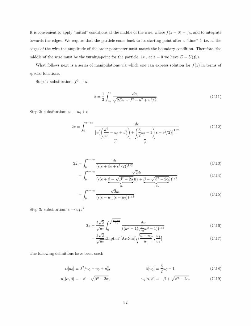
It is convenient to apply “initial” conditions at the middle of the wire, where f(z = 0) = f0, and to integrate

towards the edges. We require that the particle come back to its starting point after a “time” b, i.e. at the

edges of the wire the amplitude of the order parameter must match the boundary condition. Therefore, the

middle of the wire must be the turning-point for the particle, i.e., at z = 0 we have E = U(f0).

What follows next is a series of manipulations via which one can express solution for f(z) in terms of

special functions.

Step 1: substitution: f2 → u

z =1

2

∫ u

u0

du√2Eu− J2 − u2 + u3/2

(C.11)

Step 2: substitution: u→ u0 + ε

2z =

∫ u−u0

0

dε[ε((J2

u0− u0 + u2

0

)

︸ ︷︷ ︸α

+

(3

2u0 − 1

)

︸ ︷︷ ︸β

ε+ ε2/2)]1/2

(C.12)

2z =

∫ u−u0

0

dε

(ε(ε+ βε+ ε2/2))1/2(C.13)

=

∫ u−u0

0

√2dε

(ε(ε+ β +√β2 − 2α︸ ︷︷ ︸−u1

)(ε+ β −√β2 − 2α︸ ︷︷ ︸−u2

))1/2(C.14)

=

∫ u−u0

0

√2dε

(ε(ε− u1)(ε− u2))1/2(C.15)

Step 3: substitution: ε→ u1z2

2z =2√

2√u2

∫ q

u−u0u1

0

dω

((ω2 − 1)(u1

u2ω2 − 1))1/2

(C.16)

=2√

2√u2

EllipticF[ArcSin

[√u− u0

u1

],u1

u2

](C.17)

The following definitions have been used:

α[u0] ≡ J2/u0 − u0 + u20, β[u0] ≡ 3

2u0 − 1, (C.18)

u1[α, β] ≡ −β −√β2 − 2α, u2[α, β] ≡ −β +

√β2 − 2α. (C.19)

92

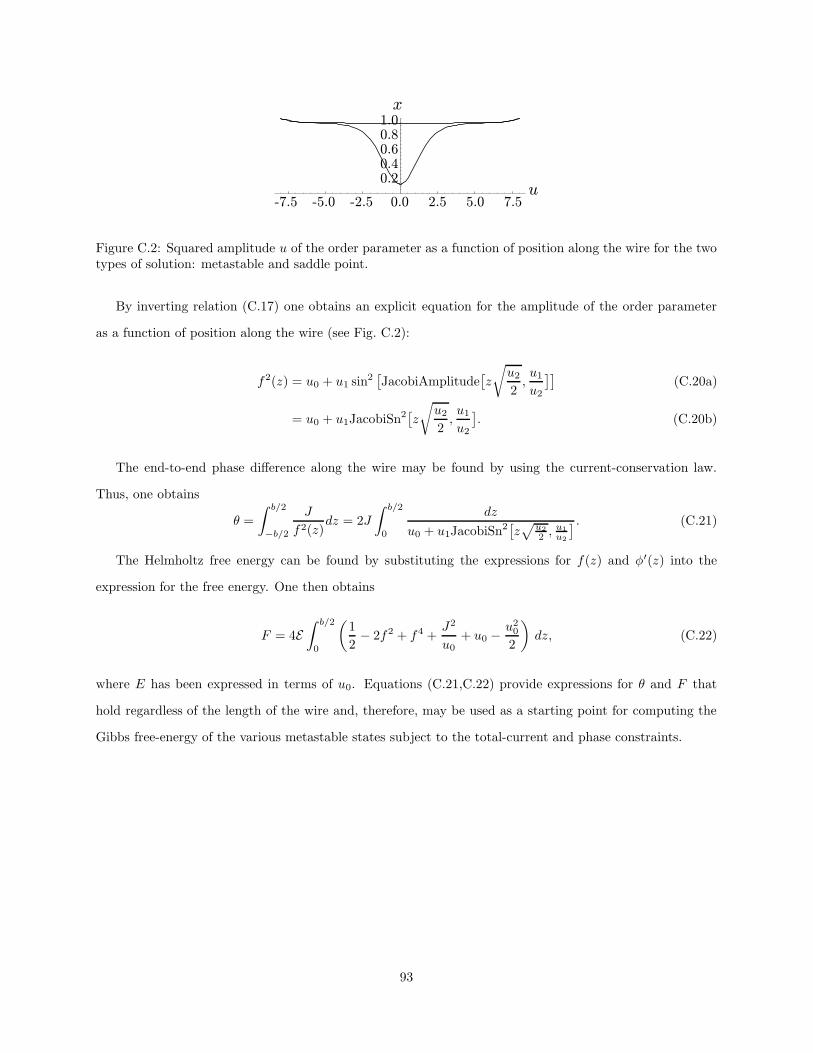
-7.5 -5.0 -2.5 0.0 2.5 5.0 7.5

0.6

0.8

0.4

1.0

0.2u

x

Figure C.2: Squared amplitude u of the order parameter as a function of position along the wire for the twotypes of solution: metastable and saddle point.

By inverting relation (C.17) one obtains an explicit equation for the amplitude of the order parameter

as a function of position along the wire (see Fig. C.2):

f2(z) = u0 + u1 sin2[JacobiAmplitude

[z

√u2

2,u1

u2

]](C.20a)

= u0 + u1JacobiSn2[z

√u2

2,u1

u2

]. (C.20b)

The end-to-end phase difference along the wire may be found by using the current-conservation law.

Thus, one obtains

θ =

∫ b/2

−b/2

J

f2(z)dz = 2J

∫ b/2

0

dz

u0 + u1JacobiSn2[z√

u2

2 ,u1

u2

] . (C.21)

The Helmholtz free energy can be found by substituting the expressions for f(z) and φ′(z) into the

expression for the free energy. One then obtains

F = 4E∫ b/2

0

(1

2− 2f2 + f4 +

J2

u0+ u0 −

u20

2

)dz, (C.22)

where E has been expressed in terms of u0. Equations (C.21,C.22) provide expressions for θ and F that

hold regardless of the length of the wire and, therefore, may be used as a starting point for computing the

Gibbs free-energy of the various metastable states subject to the total-current and phase constraints.

93

Appendix D

Josephson effect in a single aperture

We would like to consider the Josephson effect in a single 4He aperture. The setup is as follows.

• Two reservoirs of superfluid helium are joined by a single aperture.

• The aperture diameter and length are sufficiently small that its free energy may be described by the

Josephson relation.

• The pressure difference is applied across the aperture, giving rise to a chemical potential difference

that tends to drive a supercurrent.

• We assume that the at each point in time, the system is in thermodynamic equilibrium. This assump-

tion is true when the relaxation time between different modes in the superfluid is much faster than the

inverse Josephson frequency. This relaxation time may be estimated from the ratio of the reservoir

size to the speed of sound.

• The flow of supercurrent through the aperture is insufficient to fix the chemical potential imbalance

The question we would like to address is what role do the thermal fluctuations in the superfluid play? What

happens when kBT is on the order of Josephson energy for the Junction EJ? Do thermal fluctuations destroy

the Josephson effect?

We assume that there is a well-defined phase difference between the left and right reservoirs. When

a chemical potential difference is applied between the reservoirs, the relative phase between them winds

according to the Josephson-Anderson relation:

ϕ(t) = −1

~∆µ(t). (D.1)

Where is this phase difference specified? The only possible location to set the phase difference is far away

from the aperture, where, due to long range order in 3D superfluid, it makes sense to specify values of phase

differences. Without loss of generality, to simplify the calculations we consider two spherical reservoirs of

94

radius R, connected by an aperture of radius r0 (it is, of course, not possible to embed this setup into

three dimensional space, but the qualitative behavior is identical to the more realistic setup described in

Chapter 3). The phase of the order parameter in the left and right spheres, ϕL(r) and ϕR(r), will be set on

the outer walls, as follows:

ϕL(r = R,Ω) = ϕL0 , ϕR(r = R,Ω) = ϕR

0 . (D.2)

To determine if the Josephson effect persists in spite of thermal fluctuations, we shall fix the phases ϕL0

and ϕR0 deep in the bulk superfluids, and look for a Josephson supercurrent through the aperture.

D.1 Partition function

Next, we need to obtain the partition function describing the superfluid in the reservoirs as well as in the

aperture. Here, we will take a different approach than in the main text to coupling the superfluid in the two

reservoirs through the aperture. Similar to the main text, we assume that the energy of the superfluid in the

aperture can be described by a single variable — the phase difference across it. However, instead of joining

the description of the superfluid in the bulk and in the aperture on a surface enclosing the aperture opening

we take a different strategy. On each side of the aperture we compute the weighted average of the phase

of the bulk superfluid, with the weighting function T (r) that is concentrated near the aperture openings.

Next, we set the phase across the aperture to be the difference of these weighted averages. (Alternatively,

we could consider a point aperture and introduce some ultraviolet cut-off of in the k sums, but what we do

amounts to the same thing, with the cut-off scale being set by the inverse of the aperture radius r0. It is

important to note that this trick only works for non-extended Josephson junctions, i.e. when ξ & r0.)

Using the energy functional for the bulk superfluids from the main text, and the averaging procedure for

connecting the aperture to the bulk superfluids, we obtain the partition function

Z =

∫D[ϕL, ϕR, φ, ζ]

ϕL(R)=ϕL0 , ϕR(R)=ϕR

0

e−β[R

R

0(∇ϕL)2+(∇ϕR)2 d3r+iζ(φ−

R

R

0T (r)(ϕL(r)−ϕR(r)) d3r)−J cos φ], (D.3)

where T (r) is the normalized tempering function that describes how to weigh the average value of ϕ(r) in the

vicinity of the aperture, and ζ is a Lagrange multiplier used to enforce the condition that the phase across

the aperture φ matches the difference of the weighted averages∫ R

0T (r)(ϕL(r)−ϕR(r)) d3r. It is convenient

to transform to normal modes of the reservoir. As only the isotropic (l = 0 modes) can couple through

the junction (all the other modes do not survive the averaging by the isotropic wighting function), we may

95

ignore all the other modes. Furthermore, we take the opportunity to enforce the boundary condition, and

write:

ϕL/R(r) = ϕL/R0 +

1√2πR

∑

k=πn/R

AL/Rk

sin(kr)

r(n = 1, 2, . . .). (D.4)

These form an orthonormal basis set, except for the k = 0 mode which is orthogonal but not normal, as can

be easily verified:

1

2πR

∫ R

0

4πr2 drsin(kr)

r

sin(k′r)

r= δk,k′ . (D.5)

Furthermore, we can show that modes are not coupled by the kinetic energy term

1

2πR

∫ R

0

4πr2 dr

(∂r

sin(kr)

r

)(∂r

sin(k′r)

r

)= k2δk,k′ . (D.6)

Finally, we make a convenient choice of the tempering function and take the inner product. We believe that

the exact form of the tempering function is unimportant, so it is convenient to choose:

T (r) =e−r/r0

r

(∫ R

0

4πr2e−r/r0

rdr

)−1

. (D.7)

The inner product of T (r) and one of the basis functions is given by:

∫ R

0

4πr2√2πR

sin(kr)

rT (r) dr =

2√2πR

k

1 + k2r20(D.8)

Using the basis set Eq. (D.4), we express the partition function as

Z =

∫D[AL

k , ARk , φ, ζ] exp−β

[∑

k>0

k2(ALk

2+AR

k

2) + iζ

φ−

(ϕL

0 − ϕR0 +

2√2πR

∑

k>0

(ALk −AR

k )k

1 + k2r20

)− J cosφ

],

(D.9)

Performing the Gaussian integrals over the Ak and Bk modes, we obtain

Z =

∫D[φ, ζ]e

−β

»

ζ2 P

k>01

πR

“

1

1+k2r02

”2

+iζ(φ−(ϕL0−ϕR

0 ))−J cos φ

–

; (D.10)

96

The mode summation may be easily evaluated for r0 R:

∑

k>0

1

πR

(1

1 + k2r02

)2

=1

4πr0+O

(r0R

)2

. (D.11)

Finally, by performing the integral over the constraint we find the effective partition function for the phase

difference across the junction:

Z[φL0 − φR

0 ] =

∫D[φ]e

−βh

πr0[φ−(ϕL0−ϕR

0 )]2−J cos φi

(D.12)

D.2 Electrostatic approach to partition function

Instead of using the above averaging procedure for joining the description of the superfluid inside the aperture

to the description in the bulk, we can follow the procedure outlined in the main text. To summarize: as the

theory for the bulk superfluid is quadratic, thermal fluctuations result in a additive constant to the effective

action as compared to its classical value. Therefore, we may compute the effective action by evaluating the

classical action and ignore the additive constant. Appealing to the electrostatic analogy, the energy of the

aperture due to coupling to the phase at infinity (i.e. due to self-capacitance) will be given by

U = 2

∫ R

0

(∇ϕ)2 d3r = 2

∫ R

r0

4πr2r20r4

(φ

2− ϕ0

2

)2

dr = 2πr0(φ− ϕ0)2, (D.13)

where the phase difference has been split between the left and right sides. This form of the action is the

same as the one that appears in the expression for the partition function Eq. (D.12) above up to a factor of

2, which arises due to different choices of how to couple the description of the superfluid in the aperture to

the description of the superfluid in the bulk.

D.3 Supercurrent

The supercurrent through the junction may be computed via

I =

∫D[φ]J sinφ e

−βh

πr0[φ−(ϕL0−ϕR

0 )]2−J cos φ

i

∫D[φ]e

−βh

πr0[φ−(ϕL0−ϕR

0 )]2−J cos φ

i (D.14)

97

If r0β 1, the current through the junction will be very strongly suppressed. This is the high temperature

limit. For the case of small J we may compute the current in perturbation theory.

I = Je−1/4πr0β sinφ0, (D.15)

if we are at high temperature, i.e. 8πr0β 1, then the formula is valid for J < 1/β; at low temperature

the range of validity is J < 8πr0.

D.4 Results

In this appendix we obtain two results. First, the mechanism for coupling the descriptions of the bulk

superfluid and the superfluid in the aperture does not seem to be very important. Second, as long as the

phase difference between the bulk superfluids is well defined, there will be a Josephson current. This current

is maintained, even for the case of very weak Josephson coupling, due to the stabilization of the phase across

the aperture by coupling to the phase at infinity. However if this coupling is also weak, than strong thermal

fluctuations of the phase across the aperture arise leading to the suppression of the Josephson effect.

98

Appendix E

Avalanche size scaling and other

critical exponents in

mean-field-theory

The goal of this appendix is to provide details of a computation of the distribution D(S) of avalanche sizes S.

In order to achieve this goal, we adopt Dahmen’s [77] calculation of avalanche-size scaling within mean-field

theory, which was done in the setting of the Random Field Ising Model, to our model of avalanches in the

superflow of helium. We note that at the mean field level, the two models are very similar with identical

critical exponents.

Our mean-field model for the dynamics of the phases across various apertures is obtained by disorder-

averaging the phase-difference across a single aperture in a self-consistent way. The half-phase difference

across the ith aperture, see Eq. (3.33) in the main text, satisfies the equation

φi =AΦ +B〈φ〉 + 4πJni

C + 4J, (E.1)

This equation must be supplemented by the condition that whenever the phase difference across an aperture

exceeds its critical value, φc,i, it phase-slips. These two conditions lead to the mean-field equation

〈φ〉 =A

A+ 4JΦ +

4πJ

A+ 4J

∑

k

k

∫ ϕk−1

ϕk

dφcQ(φc), (E.2)

where ϕk = (AΦ +B〈φ〉 − πkC)/(C + 4J). We concentrate on the “restricted” case, in which the disorder

distribution is sufficiently narrow such that |ni − nj | = 0, 1; in this setting, at any given Φ there are two

populations of apertures: the ones that have slipped n times, and the ones that have slipped n + 1 times;

the fraction of the latter will be denoted by f .

E.1 Avalanche size distribution

We would like to find the distribution of avalanche sizes, i.e., the probability that an avalanche involves

exactly S apertures. To approach this question, we first ask how many apertures are triggered, ntrig, if one

aperture phase-slips? The phase-slip in the initial aperture causes an increase in 〈φ〉, which in turn causes

99

the various φi’s to advance. This advance may trigger additional phase slips, as apertures are driven above

their critical velocities.

Before the initial event, we can divide the apertures into two groups, denoted by U±, U+ containing the

Nf apertures that have already slipped and U− containing the N(1 − f) apertures that have yet to slip.

From Eq. (E.1) and the definition of 〈φ〉 we obtain the equations for φ± corresponding to U±:

φ−(C + 4J)−B〈φ〉 = AΦ, (E.3)

φ+(C + 4J)−B〈φ〉 = AΦ + 4πJ, (E.4)

〈φ〉 = fφ+ + (1− f)φ−. (E.5)

Here, f must be obtained from the distribution of φc’s. In particular we obtain that

〈φ〉 =AΦ

A+ 4J+

4πJf

A+ 4J. (E.6)

When the initial aperture slips f → f + 1/N , and this causes 〈φ〉 as well as φ± to advance:

〈φ〉 → 〈φ〉 +4πJ

A+ 4J

1

N, (E.7)

φ± → φ± +B

C + 4J

4πJ

A+ 4J

1

N. (E.8)

If there are any apertures that have φc in the interval

(φ−, φ− +

B

C + 4J

4πJ

A+ 4J

1

N

), (E.9)

these apertures will be triggered to phase slip by the initial phase slip. The number of such apertures is

ntrig = N

∫ φ−+δ

φ−

Q(φc) dφc =B

C + 4J

4πJ

A+ 4JQ(φ−), (E.10)

where we have assumed that Q(φc) is a slowly varying function.

Consider an avalanche of size S. In the process of this avalanche we have that

φ− → φ− +B

C + 4J

4πJ

A+ 4J

S

N. (E.11)

To have such an avalanche, there must be exactly S − 1 secondary apertures within this interval. We shall

assume that the distribution of φc’s is uniform within this interval, with a density NQ(φ−). We can therefore

100

identify this as a Poisson process, the probability being Pν(S− 1) where ν is the expected number of events.

Thus, we have that

ν = SQ(φ−)B

C + 4J

4πJ

A+ 4J= (t+ 1)S, (E.12)

Pν(S + 1) =νS−1e−ν

(S − 1)!≈ 1√

2πS(t+ 1)S−1e−St, (E.13)

where we have used Stirling’s approximation (i.e. n! ≈√

2πn(n/e)n) in the last step. Finally, we notice (as

pointed out in Dahmen’s thesis [77]) that we are over-counting by a factor of S, as this interval may contain

two or more smaller avalanches as opposed to one big one. Therefore, the mean-field result for the avalanche

size distribution is in fact

D(S) ≈ 1

S3/2√

2πe−st2/2, (E.14)

where we have expanded for small t ≡ ntrig − 1. At criticality t = 0, and the distribution attains a −3/2

power law. As we move away from criticality, this power law gets cut off for large avalanches at the scale

S ∼ 2/t2.

E.2 Mean-field-theory in the vicinity of criticality

We would like to understand the scaling of various quantities, within mean-field-theory, near the critical

end-point point and the first-order line. In particular this will tell us how close we have to be to criticality

to obtain power-law scaling of the avalanche sizes.

Consider the susceptibility

χ ≡ d〈φ〉dΦ

, (E.15)

which describes the rate of change of the mean-field in response to the change of the control-phase Φ.

By differentiating the mean-field equation, Eq. (E.2), with respect to Φ, we obtain an expression for this

susceptibility that can be expanded about a critical point or line:

χ =A

A+ 4J

(1 +

4πJ

C + 4JQ(x)

)(1

−t(x)

), (E.16)

where x ≡ (AΦ +B〈φ〉)/(C + 4J)−φ0c . In the vicinity of an SWA, small changes in Φ cause drastic changes

101

in 〈φ〉. In particular, when Phi reaches the value at which an SWA occurs, a single phase slip will trigger a

macroscopic number of secondary phase slips through a cascade. Thus in the vicinity of an SWA t(x) → 0

and χ diverges. At fixed σ, as Φ is tuned t(x) can approach zero in two ways: either (i) by approaching the

critical end-point located at σ = σc or (ii) by approaching the first order line that stretches from σ = 0 to

σ = σc. We define Φc(σ), as the value of the control-phase at which t(x)→ 0.

How can t(x) → 0? This can happen by tuning Φ or σ. We can simplify the expression for χ in the

vicinity of criticality by expanding up to second power in x and first in σ:

χ ' −AB

C+4JA+4J

(x− xc)∂xt(xc) + 12 (x− xc)2∂2

xt(xc) + (σ − σc)∂σt(xc), (E.17)

Q(x) =e−x2/2σ2

√2πσ

, (E.18)

t(xc) = 0 =B

C + 4J

4πJ

A+ 4JQ(xc)− 1, (E.19)

∂xt(xc) =B

C + 4J

4πJ

A+ 4J

(− x

σ2

) e−x2/2σ2

√2πσ

, (E.20)

∂2xt(xc) =

B

C + 4J

4πJ

A+ 4J

(− 1

σ2+( xσ2

)2)e−x2/2σ2

√2πσ

, (E.21)

∂σt(xc) =B

C + 4J

4πJ

A+ 4J

(− 1

σ+x2

σ3

)e−x2/2σ2

√2πσ

. (E.22)

Here, we can consider two cases: the system is near the critical end-point (i.e. σ ' σc and x ' 0), or near

the first order line (i.e. σ < σc and x 6= 0).

E.2.1 Mean-field-theory in the vicinity of σc

In the case of σ ' σc, we have ∂xt(x) = 0 and we need to keep terms to second order in (x − xc):

∂〈φ〉∂Φ

' −AB

C+4JA+4J

(x − xc)2/2σ2c + r

, (E.23)

where r ≡ (σ − σc)/σc. From the definition of x, we obtain

dx

dΦ=

A

C + 4J+

B

C + 4J

d〈φ〉dΦ

. (E.24)

Expressing d〈φ〉dΦ in terms of dx

dΦ we obtain an ordinary differential equation for x(Φ, σ), which reads:

dx

dΦ

C + 4J

B− A

B= −

AB

C+4JA+4J

(x− xc)2/2σ2c + r

. (E.25)

102

Integrating both sides, and keeping terms to third order in x, we obtain:

Φ− Φc =A+ 4J

Arx +

1

6σ2c

A+ 4J

Ax3. (E.26)

Substituting x = r1/2σcy, we arrive at

y3 + 6y − 3A(C + 4J)√2πBJ

Φ− Φc

r3/2= 0, (E.27)

〈φ〉 − 〈φ〉c =

[σr1/2(C + 4J)y

(Φ− Φc

r3/2

)−A(Φ− Φc)

]/B ∼ r1/2y

(Φ− Φc

r3/2

),

(E.28)

which is the universal functional form of the dependence of the mean-field 〈φ〉 (i.e. the analog of the mag-

netization in the random field Ising model) on the control phase Φ (i.e. the analog of the applied magnetic

field). From this relation, we can obtain the susceptibility as well as corrections to the power law scaling of

avalanche sizes away from the critical point.

E.2.2 Mean-field-theory for σ < σc

In the case σ < σc, we cannot ignore ∂xt(xc) term, which now dominates the scaling. In this regime, near

criticality the susceptibility obeys:

∂〈φ〉∂Φ

' C + 4J

B

Aσ2

xc(A+ 4J)(x− xc)=C + 4J

B

(dx

dΦ− A

C + 4J

), (E.29)

where the last equality is copied from Eq. (E.24). Reshuffling, we obtain the ordinary differential equation:

dx

dΦ=

Aσ2

xc(A+ 4J)(x− xc)+

A

C + 4J. (E.30)

Near criticality, the last term can clearly be dropped, and we find:

(x− xc) =

√2Aσ

xc(A+ 4J)(Φ− Φc)1/2, (E.31)

〈φ〉 − 〈φ〉c ∼ (Φ− Φc)1/2. (E.32)

103

E.2.3 Mean-field equations for the critical line

Finally, we may ask how Φc(σ) behaves in the vicinity of σc. By using the condition for criticality t(xc) = 0,

we obtain the relation

xc(σ) = σ√−2 log(σ/σc). (E.33)

By using the definition for x and the mean-field-theory equation, Eq. (E.2), we obtain an equation for the

line of SWAs, i.e. Φc(σ):

〈φ〉c(σ) =1

B((xc(σ) + φ0

c)(C + 4J)−AΦc(σ)) =1

A+ 4J

(AΦc(σ) + 2πJ

(1 + Erf

[xc(σ)√

2σ

])). (E.34)

This equation, supplemented by Eq. (E.33), can be solved numerically in a straightforward way. Alter-

natively, we can expand about critical value of disorder to obtain the equation for the first-order line of

SWAs:

Φc(σ) − Φc(σc) = − 8BJ√π

3A(C + 4J)|r|3/2; (E.35)

see Fig. 3.7.

104

Appendix F

The renormalization group

transformation of the long-range

soft-spin RFIM

The goal of this appendix is to provide the details of the renormalization-group transformation of the long-

range soft-spin RFIM effective action given in Eq. (3.71). The renormalization procedure follows the same

steps as for the short-range soft-spin RFIM as described in [77], and is performed in two parts: first, the high

momentum modes lying in the range Λ/b < q < Λ, where Λ is the high-momentum cut-off and b determines

the coarse graining, are traced out; second, the lengths are rescaled by b−1 to bring the effective action back

to its original form but with rescaled coefficients.

We begin by explicitly writing the high momentum cut-off Λ in the expression for the effective action

Eq. (3.71):

Seff = −∫dt

∫ Λ

0

dq η(−q, t)[−a ∂t

Γ0+ |q| − w

]η(q, t) (F.1)

+1

2

∫dt1 dt2

∫ Λ

0

dq u2,0η(−q, t1)η(q, t2) (F.2)

+1

6

∫dt

∫ Λ

0

dq1 dq2 dq3 u η(q1, t)η(q2, t)η(q3, t)η(−q1 − q2 − q3, t). (F.3)

The cut-off Λ starts out representing the discrete nature of the aperture array (or the spins of the RFIM).

In the first step of the renormalization-group transformation we must trace over the fields with momenta in

the shell Λ/b < q < Λ, where b is some number close to, but bigger than, unity. It is convenient to introduce

the notation where we add the subscript “s” (which stands for slow) to fields with q < Λ/b and “f” (which

stands for fast) to fields with q > Λ/b. The goal then becomes to compute the effective action which is

obtained by tracing over the fast fields

exp (−βS′eff[ηs, ηs]) =

∫D[ηf, ηf] exp (−βSeff[ηs, ηs, ηf, ηf]) . (F.4)

To perform the path integral over the non-quadratic parts of the action we expand the exponential in powers

of u2,0 and u to one loop order. At this order there are no diagrams that correspond to the the rescaling of

u2,0. The Feynman diagrams describing the rescaling of w and u are pictured in Fig. 3.10. The corresponding

105

amplitudes of these two diagrams are

A1 =1

2u2,0uI1 ≡

1

2

∫ Λ

Λ/b

dq1

(|q| − w)2u2,0u (F.5)

for the rescaling of w (top diagram) and

A2 =1

2u2,0u

2I2 ≡1

2

∫ Λ

Λ/b

dq1

(|q| − w)3u2,0u

2 (F.6)

for the rescaling of u (bottom diagram). Therefore, upon integrating over the fast fields we are left with the

effective action

Seff = −∫dt

∫ Λ/b

0

dq η(−q, t)[−a ∂t

Γ0+ |q| −

(w +

1

2I1u2,0u

)]η(q, t) (F.7)

+1

2

∫dt1 dt2

∫ Λ/b

0

dq u2,0η(−q, t1)η(q, t2) (F.8)

+1

6

∫dt

∫ Λ/b

0

dq1 dq2 dq3 (u+ 3I2u2,0u2) η(q1, t)η(q2, t)η(q3, t)η(−q1 − q2 − q3, t). (F.9)

Next we perform the second step of the renormalization-group transformation and rescale the length so

as to bring the effective action Eq. (F.9) to the original form Eq. (F.3). After this transformation, we find

that the coefficients w and u scale as

w′ = b(w +

u2,0u

2I1), (F.10)

u′ = bε(1 + 3u2,0uI2

). (F.11)

As u always appears in combination with u2,0, it is convenient to change variables from u to v ≡ u2,0u. The

final step needed to obtain the renormalization-group flow equations is to evaluate the integrals I1 and I2.

We concentrate on the case of d ∼ 3, and evaluate the integrals in d = 3− ε dimensions as follows:

I1 ≈1

2π2

∫ Λ

Λ/b

dq

(1 + 2

w

q+ . . .

)=

1

2π2

[Λ

(1− 1

b

)+ 2w log b

]+O

(1

Λ

)(F.12)

I2 ≈1

2π2

∫ Λ

Λ/b

dq

q

(1 + 3

w

q+ . . .

)=

1

2π2log(b) +O

(1

Λ

). (F.13)

106

We thus arrive at the following set of flow equations:

v′ = v + v log(b)

(ε+

3v

2π2

), (F.14)

w′ = b

(w +

v

2

1

2π2

[Λ

(1− 1

b

)+ 2w log b

]). (F.15)

The flow equations, Eqs. (F.14) and (F.15), have two fixed points. The Gaussian fixed point is located

at v = 0 and u = 0 and the Wilson-Fisher fixed point at v = − 2π2

3 ε and w = εΛ6

11−ε/3 .

To facilitate further analysis, and in particular to compute critical exponents, we linearize the recursion

relations in the vicinity of the fixed points. For the Gaussian fixed point we find

∂w′

∂w∂w′

∂v

∂v′

∂w∂v′

∂v

=

b Λ

4π2 (b− 1)

0 bε

, (F.16)

where we have used 1 + ε log b = 1 + log(1 + (bε − 1)) ≈ bε. Similarly for the Wilson-Fisher fixed point we

find

∂w′

∂w∂w′

∂v

∂v′

∂w∂v′

∂v

=

b1−ε/3 Λ

4π2 (b− 1)

0 b−ε

. (F.17)

For the Gaussian fixed point the eigenvalues of this linearized transformation are ew = byt = b1 and

e2 = bε, and the corresponding eigendirections are (1, 0) and (−Λ(2π)−2, 1). The eigenvalue ew is always

bigger than unity, and therefore corresponds to an eigendirection that is always unstable. On the other

hand, e2 is smaller than unity for d > 3 and larger for d < 3. Thus for d > 3, e2 corresponds to a stable

eigendirection, while for d < 3 an unstable one.

Similarly, for the Wilson-Fisher fixed point the eigenvalues are ew = byt = b1−ε/3 and e2 = b−ε, and the

eigendirections coincide with those found for the Gaussian fixed point. Again, the eigenvalue ew is always

bigger than unity, and therefore corresponds to an eigendirection that is always unstable. For the case of the

Wilson-Fisher fixed point, however, e2 has the opposite behavior as compared to the Gaussian fixed point.

For d > 3, e2 is larger than unity and corresponds to an unstable eigendirection, while for d < 3 e2 becomes

smaller than unity and thus corresponds to a stable eigendirection.

107

References

[1] V. L. Ginzburg and L. D. Landau, Zh. Eksp. Teor. Fiz. 20, 1064 (1950).

[2] J. Bardeen, L. N. Cooper, and J. R. Schrieffer, Phys. Rev. 108, 1175 (1957).

[3] Y. M. Ivanchenko and L. A. Zil’berman, JETP Lett. 8, 113 (1968).

[4] Y. M. Ivanchenko and L. A. Zil’berman, JETP 28, 1272 (1969).

[5] V. Ambegaokar and B. I. Halperin, Phys. Rev. Lett. 22, 1364 (1969).

[6] J. S. Langer and V. Ambegaokar, Phys. Rev. 164, 498 (1967).

[7] D. E. McCumber and B. I. Halperin, Phys. Rev. B 1, 1054 (1970).

[8] W. Meissner and R. Ochsenfeld, Naturwissenschaften 21, 787 (1933).

[9] F. London and H. London, Proc. R. Soc. London, Ser A A149, 71 (1935).

[10] L. P. Gorkov, Zh. Eksp. Teor. Fiz. 34, 735 (1953), [Sov. Phys. JETP 7, 505 (1958)].

[11] L. P. Gorkov, Zh. Eksp. Teor. Fiz. 36, 1918 (1959), [Sov. Phys. JETP 9, 1364 (1959)].

[12] E. Maxwell, Phys. Rev. 78, 477 (1950).

[13] C. A. Reynolds, B. Serin, W. H. Wright, and L. B. Nesbitt, Phys. Rev. 78, 487 (1950).

[14] H. Frohlich, Phys. Rev. 79, 845 (1950).

[15] W. H. Keesom and A. P. Keesom, Physica 2, 557 (1935).

[16] W. H. Keesom and A. P. Keesom, Physica 3, 359 (1936).

[17] J. F. Allen, R. Peierls, and M. Z. Uddin, Nature 140, 62 (1937).

[18] P. Kapitza, Nature 141, 74 (1938).

[19] J. F. Allen and A. D. Misener, Nature 141, 75 (1938).

[20] J. F. Allen and H. Jones, Nature 141, 243 (1938).

[21] D. Shoenberg, Nature 171, 458 (1953).

[22] L. P. Pitaevskii, J. Low Temp. Phys. 87, 127 (1992).

[23] L. D. Landau, J. Phys. U.S.S.R. 5, 71 (1941).

[24] E. P. Gross, Nuovo Cimento 20, 454 (1961).

[25] E. P. Gross, J. Math. Phys. 4, 195 (1963).

[26] L. P. Pitaevskii, JETP 13, 451 (1961).

108

[27] M. P. A. Fisher and W. Zwerger, Phys. Rev. B 32, 6190 (1985).

[28] A. O. Caldeira and A. J. Leggett, Physica A 121, 587 (1983).

[29] W. A. Little, Phys. Rev. 156, 396 (1967).

[30] D. E. McCumber, Phys. Rev. 172, 427 (1968).

[31] P. W. Anderson, Rev. Mod. Phys. 38, 298 (1966).

[32] W. A. Little and R. D. Parks, Phys. Rev. Lett. 9, 9 (1962).

[33] W. A. Little and R. D. Parks, Phys. Rev. 133, a 97 (1964).

[34] M. Tinkham, Introduction to Superconductivity, 2nd ed. (McGraw-Hill, New York, 1996).

[35] K. K. Likharev, Rev. Mod. Phys. 51, 101 (1979).

[36] A. Bezryadin and B. Pannetier, J. Low Temp. Phys. 98, 251 (1995).

[37] C. C. Abilio, L. Amico, R. Fazio, and B. Pannetier, J. Low Temp. Phys. 118, 23 (2000).

[38] D. S. Hopkins, D. Pekker, P. M. Goldbart, and A. Bezryadin, Science 308, 1762 (2005).

[39] C. A. Brebbia, Boundary Element Method for Engineers (Pentech Press, London, 1978).

[40] K. K. Likharev, Sov. Radiophys. 14, 722 (1973).

[41] J. R. Clem, Bull. Am. Phys. Soc. 43, 411 (1972).

[42] G. M. Maksimova, Phys. Solid State 40, 1610 (1998).

[43] G. Stan, S. B. Field, and J. M. Martinis, Physical Review Letters 92, 097003 (2004).

[44] I. S. Gradstein and I. M. Ryzhik, Table of Integrals, Series, and Products (Academic Press, New York,1965).

[45] Zinn-Justin, Quantum Field Theory and Critical Phenomena, 3rd ed. (Oxford University Press, NewYork, 2002).

[46] R. C. Jaklevic, J. Lambe, A. H. Silver, and J. E. Mercereau, Phys. Rev. Lett. 12, 159 (1964).

[47] S. K. H. Lam and D. L. Tilbrook, Appl. Phys. Lett. 82, 1078 (2003).

[48] J.-P. Cleuziou, W. Wernsdorfer, V. Bouchiat, T. Ondarcuhu, and M. Monthioux, Nature Nanotech. 1,53 (2006).

[49] I. Chiorescu, Y. Nakamura, C. J. P. M. Harmans, and J. E. Mooij, Science 299, 1869 (2003).

[50] W. Wernsdorfer et al., Phys. Rev. Lett. 79, 4014 (1997).

[51] W. Wernsdorfer and R. Sessoli, Science 284, 133 (1999).

[52] D. S. Hopkins, Measurements of superconducting phase gradients by a nanowire quantum interferencedevice templated by DNA molecules, PhD thesis, University of Illinois at Urbana Champaign, 2007.

[53] J. Bardeen, Rev. Mod. Phys. 34, 667 (1962).

[54] S. J. Turneaure, T. R. Lemberger, and J. M. Graybeal, Phys. Rev. Lett. 84, 987 (2000).

[55] R. Prozorov et al., Phys. Rev. B 67, 184501 (2003).

[56] A. M. Campbell, J. Phys. C 2, 1492 (1969).

109

[57] A. M. Campbell, J. Phys. C 4, 3186 (1971).

[58] R. Labusch, Phys. Rev. 170, 470 (1968).

[59] M. Tinkham and C. N. Lau, Applied Physics Letters 80, 2946 (2002).

[60] B. J. Baelus, A. Kanda, F. M. Peeters, Y. Ootuka, and K. Kadowaki, Physical Review B (CondensedMatter and Materials Physics) 71, 140502 (2005).

[61] K. Y. Arutyunov and T. T. Hongisto, Physical Review B (Condensed Matter and Materials Physics)70, 064514 (2004).

[62] A. A. Pesetski and T. R. Lemberger, Phys. Rev. B 62, 11826 (2000).

[63] A. Lamacraft and B. D. Simons, Phys. Rev. Lett. 85, 4783 (2000).

[64] M. Hermele, G. Refael, M. P. A. Fisher, and P. M. Goldbart, Nature Physics 1, 117 (2005).

[65] Y. Sato, E. Hoskinson, and R. E. Packard, Physical Review B (Condensed Matter and MaterialsPhysics) 74, 144502 (2006).

[66] K. Sukhatme, Y. Mukharsky, T. Chui, and D. Pearson, Nature 411, 280 (2001).

[67] E. Hoskinson, R. E. Packard, and T. M. Haard, Nature 433, 376 (2005).

[68] E. Hoskinson, Y. Sato, I. Hahn, and R. E. Packard, Nature Physics 2, 23 (2006).

[69] R. P. Feynman, Progress in Low Temperature Physics (North-Holland, Amsterdam, 1955), Vol. 1,Chap. 2.

[70] S. V. Iordanskii, Zh. Eksp. Teor. Fiz. 48, 708 (1965), [Sov. Phys. JETP 21 467-471 (1965)].

[71] W. Zimmermann, in Proceedings of the Fifth Oregon Conference on Liquid Helium, a Report from theDepartment of Physics, p. 118, University of Oregon, 1987.

[72] T. Chui, W. Holmes, and K. Penanen, Phys. Rev. Lett. 90, 085301 (2003).

[73] R. Burridge and L. Knopoff, Bull. Seismol. Soc. Am. 57, 341 (1967).

[74] J. P. Sethna et al., Phys. Rev. Lett. 70, 3347 (1993).

[75] D. S. Fisher, Phys. Reps. 301, 113 (1998), see for a review.

[76] M. C. Marchetti, cond-mat/0503660 (2005), see also and references therein.

[77] K. Dahmen, Hysteresis, Avalanches, and Disorder-Induced Critical Scaling: A Renormalization GroupApproach, PhD thesis, Cornell, 1995.

[78] J. C. Davis and R. E. Packard, Rev. Mod. Phys. 74, 741 (2002).

[79] B. D. Josephson, Phys. Lett. 1, 251 (1962).

[80] J. M. Rowell, Phys. Rev. Lett. 11, 200 (1963).

[81] I. Giaever, Phys. Rev. Lett. 14, 904 (1965).

[82] M. Albiez et al., Physical Review Letters 95, 010402 (2005).

[83] O. Avenel and E. Varoquaux, Phys. Rev. Lett. 60, 416 (1988).

[84] S. Backhaus, S. V. Pereverzev, A. Loshak, J. C. Davis, and R. E. Packard, Science 278, 1435 (1997).

[85] G. B. Hess, Phys. Rev. Lett. 27, 977 (1971).

110

[86] O. Narayan and D. S. Fisher, Phys. Rev. Lett. 68, 3615 (1992).

[87] O. Narayan and D. S. Fisher, Phys. Rev. B 46, 11520 (1992).

[88] P. C. Martin, E. D. Siggia, and H. A. Rose, Phys. Rev. A 8, 423 (1973).

[89] K. Dahmen and J. P. Sethna, Phys. Rev. Lett. 71, 3222 (1993).

[90] K. Dahmen and J. P. Sethna, Phys. Rev. B 53, 14872 (1996).

[91] H. Sompolinsky and A. Zippelius, Phys. Rev. B 25, 6860 (1982).

[92] Y. Sato, Model of thermal fluctuations, private communication.

111

Author’s Biography

David Pekker was born in a typical Soviet scientific family and grew up in Novosibirsk, central Siberia,

Russia. In 1991, his family immigrated to the U.S., first settling in St. Paul, Minnesota, and later moving

to Austin, Texas. He received his B.S. in Physics and B.A. in Mathematics in 2002 from Rice University, in

Houston, Texas. He entered the Ph.D. program in Physics at the University of Illinois at Urbana Champaign

in 2002.

List of publications at the University of Illinois at Urbana-Champaign

1. D. Pekker, R. Barankov, and P. M. Goldbart “Critical properties of dissipative superflow of helium in

multiply-connected geometries,” in preparation (2007).

2. D. Pekker, R. Barankov, and P. M. Goldbart “Phase-slip avalanches in the superflow of 4He through

arrays of nanosized apertures,” Physical Review Letters , (2007).

3. A. Rogachev, T.-C. Wei, D. Pekker, A.T. Bollinger, P. M. Goldbart, and A. Bezryadin, “Magnetic field

enhancement of superconductivity in ultra-narrow wires,” Physical Review Letters 97, 137001 (2006).

4. T.-C. Wei, D. Pekker, A. Rogachev, A. Bezryadin, P. M. Goldbart “Enhancing superconductivity:

Magnetic impurities and their quenching by magnetic fields,” Europhysics Letters 75, 943 (2006).

5. D. Pekker, A. Bezryadin, D. S. Hopkins, and P. M. Goldbart, “Operation of a superconducting nanowire

quantum interference device with mesoscopic leads,” Physical Review B 72, 104517 (2005).

6. D. Pekker, S. Mukhopadhyay, N. Trivedi, and P. M. Goldbart, “Double-exchange model for nonin-

teracting electron spins coupled to a lattice of classical spins: Phase diagram at zero temperature,”

Physical Review B 72, 075118 (2005).

7. D. S. Hopkins, D. Pekker, P. M. Goldbart, and A. Bezryadin, “Quantum Interference Device Made by

DNA Templating of Superconducting Nanowires,” Science 308 1762 (2005).

112