POWER SYSTEM STABILITY ENHANCMENT USING UPFC DAMPING CONTROLLER

A Thesis submitted in partial fulfillment of the requirements for

the degree of Master of Technology

In

Electrical Engineering

(Power Electronics and Drives)

By

Sudhansu Kumar Samal

Roll Number: 212EE4512

DEPARTM ENT OF ELECTRICAL ENGINEERING NATIONAL INSTITUTE OF TECHNOLOGY,

ROURKELA ODISHA, INDIA PIN-769008

(2012-2014)

POWER SYSTEM STABILITY ENHANCMENT USING UPFC DAMPING CONTROLLER

By

Sudhansu Kumar Samal

Roll Number. 212EE4512

DEPARTM ENT OF ELECTRICAL ENGINEERING NATIONAL INSTITUTE OF TECHNOLOGY,

ROURKELA ODISHA, INDIA PIN-769008

(2012-2014)

Dedicated to

My beloved Parents

NATIONAL INSTITUTE OF TECHNOLOGY ROURKELA

CERTIFICATE

This is to certify that the thesis report entitled “Power System Stability Enhancement

Using UPFC Damping Controller” submitted by Mr. Sudhansu Kumar Samal in partial

fulfillment of the requirements for the award of Master of Technology degree in

Electrical Engineering with specialization in “Power Electronics and Drives” during

session 2012-2014 at National Institute of Technology, Rourkela (Deemed University)

and is an authentic work by him under my supervision and guidance.

To the best of my knowledge, the matter embodied in the thesis has not been submitted to

any other university/institute for the award of any degree or diploma.

Prof. P. C. PANDA

Date: Dept. of Electrical Engineering

Place: Rourkela NIT Rourkela

i

I would like to appearance my extreme gratitude to my supervisor Prof. P. C. Panda,

Professor, Department of Electrical Engineering, NIT Rourkela. I feel encouraged and

motivated every time I meet him. Without his inspiration and supervision, this project would

not have materialized.

I am also thankful to Prof. A. K. Panda for his valuable suggestions towards the completion of

my project. I would like to thank Rakhi Panigrahi and Rajendra Prasad and my friend Saroj

and Biranchi for their help and moral support. Finally I would like to thank my Parents and

elder Sister Shantilata Samal for their moral support and encouragement.

Apart after my hard work, the accomplishment of any project depends highly on the

inspiration and guidance of several others. I yield this opportunity to express my gratitude to

the people who have been instrumental in the successful achievement of this project.

The guidance and provision acknowledged from all the associates who help and who are

backing to this project, was vital for the achievement of the project. I am very much obliged

for their continuous support and assistance.

SUDHANSU KUMAR SAMAL

Roll No: 212EE4512

ii

ABSTRACT

The rising of demand of power and difficulties of constructing a newly transmission network

causes the power system to be complex and stressed. Due to the stress in the power system

there is a chance of losing the stability following to the fault. When the fault occurs in the

power system the whole system goes to severe transients. By using PSS and AVR we can

easily stabilize the system. FACTS devices (i.e. TCSC, SVC, STATCOM, and UPFC) are

extremely important to suppressing the power system oscillations for faults and it also

increasing the damping of the system. The power electronic device named as UPFC which

efficiently control the active and reactive power. This thesis reflects a novel control technique

which is based on Fuzzy Logic technique to provide external controlling signal to UPFC

which is mounted in a single-machine infinite bus system to suppress low frequency

oscillations and also it describes the model of a UPFC with multi-machine system which is

externally controlled by the signal which is generated by the newly proposed power flow

controller to increase the stability of the system with occurrence of fault in which it

connected. The proposed controller consists of Power oscillation damping controller and

Proportional Integral Differential controller (POD & PID). The effectiveness of controller for

suppressing oscillation due to change in mechanical input and excitation is examined by

investigating their change in rotor angle and speed occurred in the SMIB system. FACTS

devices are used the existing transmission system very efficiently with the specified stability

margin.

iii

LIST OF FIGURES

FIGURE NO FIGURE TITLE PAGE NO

1.1 Schematic diagram of FACTS controllers…………………….. 06

2.1 Single Machine Infinite Bus systems ...………………………..11

2.2 Block diagram representation of small signal SMIB model…... 14

2.3 Simplified SMIB model for Heffron-Philips model…………....16

2.4 The linearized Heffron-Philips model…………………………..18

2.5 A two-voltage source UPFC model……………………………..18

2.6 UPFC injected voltage model …………………………………..19

2.7 A UPFC installed in SMIB system……………………………...21

2.8 Heffron-Philips model of SMIB system with UPFC …………..21

2.9 Conventional Power System Stabilizer………………………....22

2.10 UPFC with Power System Stabilizer …………………………..23

2.11 Basic structure of Fuzzy Controller……………………………..24

2.12 UPFC with Fuzzy Logic Controller……………………………..24

2.13 Hybrid fuzzy damping controller structure……………………...26

2.14 Response of SMIB system without UPFC………………………27

2.15 Response of SMIB system with UPFC………………………….28

2.16 Response of SMIB system with UPFC and Power

System Stabilizer………………………………………………...29

2.17 Response of SMIB system with UPFC and Conventional

Fuzzy Logic Controller ………………………………………….30

2.18 Response of SMIB system with UPFC and Hybrid Fuzzy

Logic Controller………………………………………………....31

2.19 Comparison of Response of SMIB system without and

with UPFC with various controllers …………………………...32

3.1 Connection diagram of UPFC with transmission line…………...36

3.2 A general circuit equivalent of UPFC …………………………...36

iv

FIGURE NO FIGURE TITLE PAGE NO

3.3 UPFC based control system…………………………………….37

3.4 Single line diagram of two-machine power

system with UPFC controller ………………………………….38

3.5 Block diagram of PID controller Parameters…………………..39

3.6 PID controller in proportional action…………………………..39

3.7 Determination of sustained oscillation (Pcr)………………….. 39

3.8 PID controller with tuning parameters………………………....39

3.9 Internal structure of PID controller with dω1& dω2 input ……40

3.10 Internal structure of POD controller…………………………...41

3.11 Complete model of Power System Controller…………………41

3.12 Bus voltage (B1) in p.u. without UPFC………………………..42

3.13 Bus power (B1) in MW without UPFC………………………..42

3.14 Bus voltage in p.u. (UPFC without power flow controller) …..43

3.15 Bus power in MW (UPFC without power flow controller)……43

3.16 Bus voltage (B1) in p.u. without UPFC………………………..43

3.17 Bus power (B1) in MW without UPFC………………………..44

3.18 Bus voltage in p.u. (UPFC without power flow controller) …..44

3.19 Bus power in MW (UPFC without power flow controller)……44

3.20 Bus voltage in p.u. (UPFC with power system controller)…….45

3.21 Bus power in MW (UPFC with power system controller)…….45

3.22 Bus voltage in p.u. (UPFC with power system controller) ……45

3.23 Bus power in MW (UPFC with power system controller)…….46

v

LIST OF TABLES TABLE NO TABLE TITLE PAGE NO

Table.1 Comparison of Response of SMIB system

with out and with UPFC with various controllers…………..33

Table.2 The performance of UPFC with Power Flow

Controller having same 500KV transmission line……….....46

vi

ABBREVIATION

FACTS : Flexible AC Transmission Systems

TCSC : Thyristor Controlled Series Capacitor

SSSC : Static Synchronous Series Compensators

UPFC : Unified Power Flow Controllers

PSS : Power System Stabilizer

VSC : Voltage Source Converter

LFO : Low Frequency Oscillation

PFC : Power Flow Controller

ANN : Artificial Neural Network

POD : Power Oscillation damping

S-L-G : Single-Line-Ground

PID : Proportional Integral Derivative

SVC : Static VAR Compensator

STATCOM : Static Synchronous Compensators

vii

ABSTRACT

LIST OF FIGURES

LIST OF TABLES

ABBREVIATION

CONTENTS

CHAPTER 1

INTRODUCTION

1.1 Introduction

1.2 Power System Stability

1.3 Transient Stability

1.4 FACTS Devices

1.4.1 Flexible AC Transmission System (FACTS)

1.4.2 FACTS Controller

1.5 Literature Review

1.6 Problem Formulation

1.7 Objectives and Scope of the Project

1.8 Organization of the Thesis

CHAPTER 2

MODELING OF UPFC FOR SMALL SIGNAL STABILITY ANALYSIS OF SMIB

(HEFFRON-PHILIPS MODEL) SYSTEM.

2.1 Introduction

2.2 Small Signal Stability of SMIB System

2.3 Modeling of Small Signal Stability of SMIB System (Heffron-Philips Model)

2.4 Steady-State Model of the UPFC

2.5 Dynamic Model of the UPFC

2.6 Power system stabilizer

2.7 Fuzzy Logic Controller

2.7.1 Hybrid Fuzzy Controller

2.8 Simulation Results and Discussion

viii

CHAPTER 3

POWER SYSTEM OSCILLATION DAMPING USING UPFC COORDINATED WITH POD

AND PID CONTROLLERS.

3.1 Introduction

3.2 control concept of UPFC

3.3 UPFC based control system

3.4 Power system model with UPFC

3.5 Design of power flow controller (PID and POD)

3.5.1 Design of PID controller

3.5.2 Design of POD controller

3.6 Simulation Results and Discussion

CHAPTER 4

CONCLUSION AND SCOPE FOR FUTURE WORK

4.1 Conclusion

4.2 Future Scope

REFERENCES

PUBLICATION

1

CHAPTER 1

INTRODUCTION

2

CHAPTER 1

1.1 Introduction – Now recent years, the power system design, high efficiency operation and

reliability of the power systems have been considered more than before. Due to the growth in

consuming electrical energy, the maximum capacity of the transmission lines should be

increased. Therefore in a normal condition also the stability as well as the security is the

major part of discussion. Several years the power system stabilizer act as a common control

approach to damp the system oscillations [1-2]. However, in some operating conditions, the

PSS may fail to stabilize the power system, especially in low frequency oscillations [3]. As a

result, other alternatives have been suggested to stabilize the system accurately. It is proved

that the FACTS devices are very much effective in power flow control as well as damping

out the swing of the system during fault. Recent years lots of control devices are implemented

under the FACTS technology. By implementing the FACTS devices gives the flexibility for

voltage stability and regulation also the stability of the system by getting proper control

signal [4].The FACTS devices are not a single but also collection of controllers which are

efficiently not only work under the rated power, voltage, impedance, phase angle frequency

but also under below the rated frequency. Among all FACTS devices the UPFC most popular

controller due to its wide area control over power both active and reactive, it also gives the

system to be used for its maximum thermal limit. It’s primarily duty to control both the

powers independently. It has been shown that all three parameters that can affect the real

power and reactive power in the power system can be simultaneously and independently

controlled just by changing the control schemes from one type to other in UPFC. Moreover,

the UPFC is executed for voltage provision and transient stability improvement by

suppressing the sub-synchronous resonance (SSR) or LFO [5]. For example, in it has been

shown that the UPFC is capable of inter-area oscillation damping by means of straight

controlling the UPFC’s sending and receiving bus voltages. Therefore, the main aim of the

UPFC is to control the active and reactive power flow through the transmission line with

emulated reactance. It is widely accepted that the UPFC is not capable of damping the

oscillations with its normal controller. As a result, the auxiliary damping controller should be

supplemented to the normal control of UPFC in order to retrieve the oscillations and improve

the system stability.

1.2 Power System Stability-The term stability exist due to the existence of the synchronous

machine in the power system .The power which is available in the real world on the

economical basis by the use of all conventional sources is all generated from synchronous

3

generator. The generators are always located at the remote end of the load or distribution

centers. And almost all or bulk quantity of power is generation is able to transmitted to the

load center by using extra high voltage lines. Stability is the capability of the system to retain

synchronism with externally connected transmission line by synchronous generator in order

to deliver maximum power to either small, sudden load change. The two important

parameters are usually defines the stability consideration are 1).supply frequency 2).The

terminal voltage. In general the active or real power is only considered for the stability

consideration, because any change in the load end is always reflects as a change in the rotor

position of alternator. Most common word resembles in the stability are the acceleration and

deceleration, moment of inertia, angular velocity, power angle etc. If we are talking about the

stability it is nothing but a virtue of the system or some part of the system to develop a

restoring force which is equal to the or greater than the disturbing force to maintain the

stability or synchronism. The maximum power which can be transmitted through the system

at any operating point is refer as a stability limit to the part of the system to which the

stability limit refers is operating with stability. Generally for the analysis purpose we are

considering three conditions.1).Steady State Stability 2).Transient Stability 3) Dynamic

stability. [1] [6].

The ability to maintain synchronism by delivering maximum amount of real power for a

small and gradual variation of load is simply termed as steady state stability. The rate of

change of load is less than rate of change of excitation controller or the frequency of

oscillation due to change of load are less than the natural frequency of the system.

If the system subject to the sudden and large variation of the load due to 3-phase short

circuit fault occurred for only a time of 5 cycles, then the maximum amount of power that can

be delivered to the load without losing the synchronism is called transient stability. If the

oscillation persist after first swing of the rotor up to the point for which the rotor regain its

new operating point to maintain the stability without losing the synchronism is called as

dynamic stability.

1.3 Transient Stability- A synchronous power system seems transient stability if

subsequently a huge, quick disturbance, it manages to recover and continue the state of

synchronism. A quick huge disturbance comprises application of different faults, switching

of the arrangement rudiments (loads, transmission lines, generators etc.).The study carried

out for the transient stability is analyzed for short time that is equivalent to the first swing of

4

the rotor. Normally the time period which we have considered is one second or less then of

that. Because it seems that if the system being stable after a first swing then we can predict

that the whole system remain stable and the proceeding swing diminish and all system are

intact. [1] [7].

Assumption to evaluate the transient stability:

1. The resistance, the shunt capacitance of generator and the transmission lines are

ignored. The shunt element like shunt capacitor (or) shunt inductor at load bus or

generator bus are ignored. The network is represented as transfer reactance.

2. The input mechanical power is assumed to be constant.

3. The speed of the alternator remains constant.

4. The damping force provided by the damper winding assumed to be neglected.

5. The reactance voltage of the machine assumed to be neglected.

The transient stability can be analyzed by using the swing equation.

Sinδ

1.4 FACTS Devices-

1.4.1-FACTS System (FACTS): It defined as AC transmission network integrating

semiconductor based power electronic device as well as different stationary controllers to

increase the capacity of power flow and also expand the controllability of the system.

1.4.2-FACTS Controller: It includes power electronic devices as well as other static devices

with advance power electronic conversion and switching capability. It is significant to describe that some other static device which is used as a controller are not

belongs to the power electronic family but basically the used controller are thyristor devices.

When we are use the FACTS as a reactive power controller they are provided with minimum

storage at dc side. The general symbol for FACTS Controller is shown in Fig. 1.2a. FACTS

Controllers are distributed into four groups [8] [9].

1] Series FACTS Controllers

2] Shunt FACTS Controllers

4] Combined Series-Shunt FACTS Controllers

3] Combined Series-Series FACTS Controllers

i) Series FACTS Controllers: - These FACTS Controllers are inject the voltage series

through the connected line , if this series injected voltage is in phase quadrature to the line

current, the controller simply deliver or receives the variable reactive power which is

5

illustrated in Fig. 1.2b. Other than the quadrature with injected voltage and line current the

controller can involve itself for real power control.

ii) Shunt FACTS Controllers: - The shunt FACTS Controllers have flexible impedance

type i.e. reactor or capacitor adjustable source based on the power electronics , which is shunt

connected to the line in order to inject variable current, as shown in Fig. 1.2c. Here up to

which the current is injected to the line voltage with phase quadrature it deliveries or absorbs

the reactive power to the system, other than that at any angle for voltage and current it well

work for the real power flow.

iii) Combined Series-Series FACTS Controllers: -, as illustrated in Fig. 1.2d. This

configuration provides autonomous series reactive power compensation for each line but also

transfers real power among the lines via power link. The presence of power link between

series controllers names this configuration as “Unified Series-Series Controller”.

iv) Combined Series-Shunt FACTS Controllers: - These are arrangement of distinct

arrangement of series and shunt controller and they connected in such way that the control of

both is much synchronized manner (Fig. 1.2e) or a UPFC connected with series and shunt

controller (Fig. 1.2f). The real or active power exchange is take place through the power dc

link when these controllers are connected to each other and also with the line.

(a) (b)

(c)

6

(d) (e)

(f)

Fig.1.1 Schematic diagram of FACTS Devices (a) Representation for FACTS Controller,

(b) Representation of Series FACTS Controller, (c) Symbolic representation of shunt

FACTS Controller, (d) Schematic of a series-series FACTS Controller, (e) organized

series and shunt Controller, (f) unified series-shunt Controller,

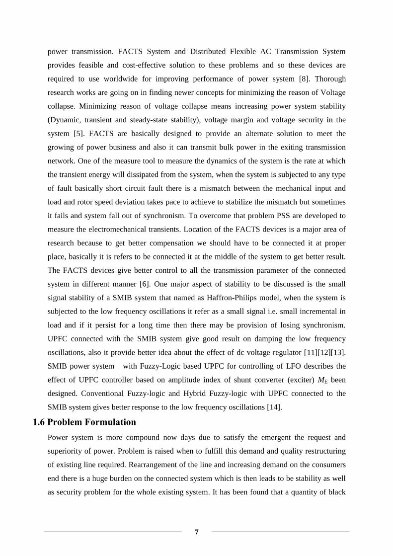
1.5 Literature Review - Power systems over the worldwide becoming complex day to day

and continuous requirements are coming for stable, secured, controlled, economic and better

quality power. These requirements become more essential when environment becoming more

vital and important deregulation. Power transfer capacity in transmission system is limited

due to various factors such as transient and steady state stability, thermal limit, damping of

the connected system. The consequence of the degree of various parameters limit are given

the electrical damping of power system require to be mitigate to steady oscillations allowed

7

power transmission. FACTS System and Distributed Flexible AC Transmission System

provides feasible and cost-effective solution to these problems and so these devices are

required to use worldwide for improving performance of power system [8]. Thorough

research works are going on in finding newer concepts for minimizing the reason of Voltage

collapse. Minimizing reason of voltage collapse means increasing power system stability

(Dynamic, transient and steady-state stability), voltage margin and voltage security in the

system [5]. FACTS are basically designed to provide an alternate solution to meet the

growing of power business and also it can transmit bulk power in the exiting transmission

network. One of the measure tool to measure the dynamics of the system is the rate at which

the transient energy will dissipated from the system, when the system is subjected to any type

of fault basically short circuit fault there is a mismatch between the mechanical input and

load and rotor speed deviation takes pace to achieve to stabilize the mismatch but sometimes

it fails and system fall out of synchronism. To overcome that problem PSS are developed to

measure the electromechanical transients. Location of the FACTS devices is a major area of

research because to get better compensation we should have to be connected it at proper

place, basically it is refers to be connected it at the middle of the system to get better result.

The FACTS devices give better control to all the transmission parameter of the connected

system in different manner [6]. One major aspect of stability to be discussed is the small

signal stability of a SMIB system that named as Haffron-Philips model, when the system is

subjected to the low frequency oscillations it refer as a small signal i.e. small incremental in

load and if it persist for a long time then there may be provision of losing synchronism.

UPFC connected with the SMIB system give good result on damping the low frequency

oscillations, also it provide better idea about the effect of dc voltage regulator [11][12][13].

SMIB power system with Fuzzy-Logic based UPFC for controlling of LFO describes the

effect of UPFC controller based on amplitude index of shunt converter (exciter) ME been

designed. Conventional Fuzzy-logic and Hybrid Fuzzy-logic with UPFC connected to the

SMIB system gives better response to the low frequency oscillations [14].

1.6 Problem Formulation

Power system is more compound now days due to satisfy the emergent the request and

superiority of power. Problem is raised when to fulfill this demand and quality restructuring

of existing line required. Rearrangement of the line and increasing demand on the consumers

end there is a huge burden on the connected system which is then leads to be stability as well

as security problem for the whole existing system. It has been found that a quantity of black

8

out have been caused by the lack of appropriate reactive power management which has to be

mitigate also one important thing to be improve is the quality of power supplied to the

distribution side.. The major problem now days are to mitigate the fault as soon as possible

or the fault clearing time should be minutest. One other thing is also creating the stability

problem is the frequent change in load demand and the excitation system.

1.7 Objectives and Scope of the Project

To study the steady state operating condition of the electrical network such as SMIB system

with low frequency oscillations for sudden load change or excitation. The steady state may be

determined by finding out the flow of active and reactive in the whole system with and

without FACTS devices. To investigate the effect of FACTS devices (basically UPFC) for

enhancing transient stability of the system to which it connected will be discussed. The

simulation results of the SMIB system are performed at different fault conditions with

different fault clearing time. Also interest is given to the finding the application of UPFC to

damping the oscillation for both single and Multi machine power system in most possible fault

clearing time.

1.8 Organization of the Thesis

Chapter 1

This chapter deliberates outline about FACTS and different FACTS Controllers, power system

stability, and transient stability, and literature review, problem formulation, objective of the

work and chapter wise contribution of the thesis.

Chapter 2

This chapter presents the Small signal analysis of SMIB, Modeling of Small Signal Stability

of SMIB System (Heffron-Philips Model), Steady State and dynamic model of the UPFC,

Power system stabilizer, conventional Fuzzy and Hybrid Fuzzy Logic Controller.

Chapter 3

This chapter presents the control concept of UPFC, UPFC based control system, Power

system model with UPFC, Design of power flow controller (PID and POD),

Chapter 4

This chapter presents the Conclusion and Scope of future scope.

9

CHAPTER 2

MODELING OF UPFC FOR SMALL SIGNAL

STABILITY ANALYSIS OF SMIB (HEFFRON-PHILIPS

MODEL) SYSTEM.

10

CHAPTER 2

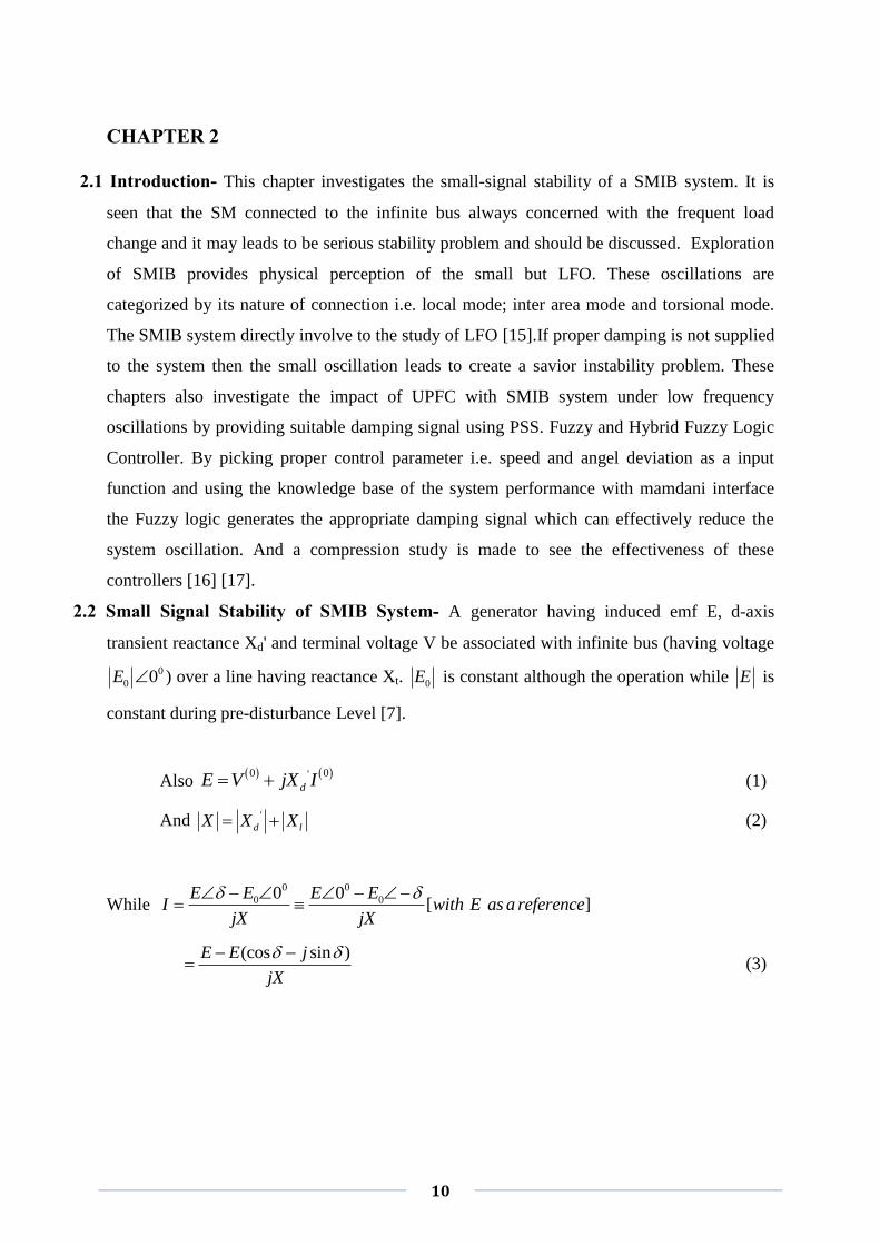
2.1 Introduction- This chapter investigates the small-signal stability of a SMIB system. It is

seen that the SM connected to the infinite bus always concerned with the frequent load

change and it may leads to be serious stability problem and should be discussed. Exploration

of SMIB provides physical perception of the small but LFO. These oscillations are

categorized by its nature of connection i.e. local mode; inter area mode and torsional mode.

The SMIB system directly involve to the study of LFO [15].If proper damping is not supplied

to the system then the small oscillation leads to create a savior instability problem. These

chapters also investigate the impact of UPFC with SMIB system under low frequency

oscillations by providing suitable damping signal using PSS. Fuzzy and Hybrid Fuzzy Logic

Controller. By picking proper control parameter i.e. speed and angel deviation as a input

function and using the knowledge base of the system performance with mamdani interface

the Fuzzy logic generates the appropriate damping signal which can effectively reduce the

system oscillation. And a compression study is made to see the effectiveness of these

controllers [16] [17].

2.2 Small Signal Stability of SMIB System- A generator having induced emf E, d-axis

transient reactance Xd' and terminal voltage V be associated with infinite bus (having voltage

0

0 0E ) over a line having reactance Xt. 0E is constant although the operation while E is

constant during pre-disturbance Level [7].

Also 0 0'

dE V jX I (1)

And '

d lX X X (2)

While 0 0

0 00 0[ ]

E E E EI with E as a reference

jX jX

(cos sin )E E j

jX

(3)

11

0 0E

0E

V

Fig 2.1 SMIB system

Where 0

V and 0I are the pre-disturbance terminal voltage and current of generator,

respectively. The generated complex power (or airgap power) at the infinite bus is obtented

as

0 0( cos )sing g g

E E E E ES P jQ EI j

X X

(4)

For the lossless generator, this air gap power or terminal power of generator

i.e. 0

sing

E EP

X (5)

In per unit, gP (generated active power) is equal to the airgap torque.

i.e. gT =

gP (in per unit system)

0

0cosg

E ET

X (6)

Assume 0 as initial operating power angle.

The swing equation of the generator rotor is given by:

2

2

0

2m e m e

HdP P T T

dt

(7)

12

[In per unit mP =

mT , while eP =

eT ,mP be the mechanical power supply to the generator while

eP be the generated output.]

It is often required to add one component of the damping torque which is proportional to the

speed deviation and swing equation is modified as follows:

2

2

0

2m e d

HdT T k

dt

(8)

Here, H =inertia constant,

0 =synchronous speed,

eT = Electrical torque (

gT ), p.u.,

mT = Mechanical torque, p.u.,

dk =damping constant.

Let r be the angular velocity of the rotor in rad/sec. If is the angular position of the rotor

in electrical radian with respect to a synchronously rotating reference and 0 is the value at

t=0, we have

0 0( )rt t

0( )r r

d

dt

(8a)

2

2

rdd d d

dt dt dt dt

To normalize the expression involving r , let us rewrite, 0

r

and then 2

02

d d

dt dt

.thus in p.u., equation (8), we can be written as

2 m e d

dH T T k

dt

(8b)

Thus, we have two equations (8a) and (8b) expressing the dynamics of rotor. Let us represent

these two equations as shown in (9a) and (9b).

From equation (8a), we can write:

0

d

dt

(9a)

And from equation (8b), we can write

1

( )2

m e d

dT T k

dt H

(9b)

13

From equation (9b) and (9a), we can write

1

( )2

m e dp T T kH

(10a)

0p (10b)

And

It might be called the speed deviation in p.u., is the rotor angle (rad), and p is the

differential operatord

dt.

Linearizing equation (10a) and using equation (6), we get

1

( )2

m e dp T T kH

i.e. 1

( )2

m c dp T T kH

(11)

Where cT the synchronizing torque coefficient and is obtained from equation (6).

0

0cosc

E ET

X (12)

Also, linearizing equation (10b), we get

0p (13)

Equations (11) and (13) can be written in a matrix from as

0

1

2 2 2

0 0

d c

m

k T

p TH H H

(14a)

Or,

Whered

xdt

,

0

2 2

0

d ck T

A H H

, x

,

1

2

0

b H

, mu T . (14b)

It may be observed that the element of state matrix A depends on dk , H, X and the initial

operating condition governed by E and 0 .figure 2.2 represents the block diagram of the

SMIB system.

14

0 0E

0E

V 1

2Hs

0

s

Fig.2.2 Block diagram representation of small signal SMIB model

From Fig. 2.2, we obtain

0 1( )

2c d mT k T

s Hs

= 0

0

1( )

2c d mT k s T

s Hs

i.e. 2 00

2 2 2

d cm

k Ts s T

H H H

(15)

The characteristic equation is then given by

2

0 02 2

d ck Ts s

H H (16)

[General form: 2 22 0n ns s ]

The undamped natural frequency is then given as

0 / sec2

n cT radH

(17)

Damping ratio ( ) is given by

0

1 1

2 2 2 2

d d

n c

k k

H T H

(18)

It may be observed that with increase in cT , the synchronizing torque coefficient, the

Natural frequency 0 increases while the damping ratio ( ) decreases. If dk is increased, the

damping ratio ( ) decreases .If dk is increased, the damping ratio ( ) increases. On the other

hand, if H is increased, n decreases along with reduction in damping ratio.

15

2.3 Modelling of Small Signal Stability of SMIB System (P-H Model) - SMIB model was

mathematically analyzed in heffron-philips model and was used extensively by Demello and

Cocordia for small signal analysis. In this model, a flux-decay system is linearized with Ed

(d-axis induced emf of a generator) as an input and then a fast acting exciter is introduced. In

the given state space model certain constant (k1 to k6) are identified: these constants are the

function of operating condition. The state space model is then used to examine the

eigenvalues as well as to design supplementary controllers to ensure adequate damping. The

real and imaginary parts of the electromechanical model are associated with the damping and

synchronizing torques [17] [18].

0 =synchronous speed in rad/sec

=steady state angular speed of the alternator in rad/sec

=angle of induced voltage (v) in rad or degree

=angle of the terminal voltage of phase voltage at terminal in p.u.

=direct axis component of the phase voltage at terminal in p.u

=quadrature axis component of phase voltage at terminal in p.u

√

=terminal voltage per phase in p.u

'

dE =direct axis component of stator induced emf in p.u

'

qE =quadrature axis component of stator induced emf in p.u

' ' 2 ' 2[ ]d qE E E =stator induced emf per phase in p.u

Id = direct axis component of armature current in p.u

Iq = quadrature axis component of armature current in p.u

Efd = open circuit terminal voltage per phase in p.u

Xd = direct axis synchronous reactance in p.u

Xq= quadrature axis synchronous reactance in p.u

'

dX = direct axis transient reactance

'

qX = quadrature axis transient reactance in p.u

H= inertia constant in seconds.

Let us draw a simplified model of SMIB (Fig.2.3). We assume the machine is connected to

the bus through an external impedance (Zl=Rl+jXl).

16

Fig.2.3 Simplified SMIB model for Heffron-Philips model.

The flux-decay model differential equation is as follows:

'

' '

'

1( )

q

q d q d fd

do

dEE X X I E

dt T (19)

0

d

dt

(20)

' '

0[ { ( ) ( )}]2

m q q d d d q d

dT E I X X I I k

dt H

(21)

The stator algebraic equations are

sin( ) 0s d q qV R I X I (22)

And ' 'cos( ) 0q s q d dE V R I X I (23)

In this model, we assume stator resistance sR =0.The equation (22 and 23) thus can be

represented as sin( ) 0q qX I V (22a)

' 'cos( ) 0q d dE V X I (23b)

Now ( )

2j j

d qV jV V

Hence, ( )

2jj

d qV jV V (24)

Expanding the RHS of the equation (24), we have

sin( ) cos( )d qV jV V jV (25)

Equating the real and imaginary parts,

sin( ); cos( )d qV V V V

Substitution of dV and qV in (22a) and (23b) yields

0q q dX I V (26)

' ' 0q q d dE V X I (27)

Cross multiplication and separation into real and imaginary parts yield

17

0 sinl d l q dR I X I V E (29)

0 cosl d l q qX I R I V E (30)

Hence ,for a SMIB model, the differential equations are given by equations(19-21) while

algebraic equations are obtained as shown in equations (26),(27),(29) and(30).The next to

linearize these equations around variables like dI , qI , , dV and

qV .

Solving for dI and

qI , we get

'

0 0 0 0

'

0 0 0 0

cos sin1

sin ( ) cos

d l q l l q q

ql l d l

I X X R E X X E E

I R R E X X E

(31)

Linearizing the three differential equations (19-21) and substituting the values ofdI , and

qI ,

we find the following equations:

''' '''

0

' ' '0 0 0 0 00 0 0 0

'

0

1 10 0 ( ) 0

0 0 1 0 0

0 ( ) ( )2 2 2 2 2

10

0 0

02

d dqdo dq

d

q

q d q d q d q d q

do

X XET TE

I

I

I k I X X X X I EH H H H H

T

H

fd

m

E

T

(32)

Substituting for dI andqI for equation (32), we get

' ' 4

' ' '

3

'0 2 0 1 0 0

1 1

2 2 2 2

q q fd

do do do

dq m

kE E E

k T T T

k k kE T

H H H H

(33)

The parameters ( 1k to 6k ) all changes with operating condition, except 3k (which is ratio of

impedance). These equations represent the linearized minor perturbation relation of a sole

generator connected with an Infinite bus through external impedance. Suffix 0 stands for

initial value. The linearized P-H model is shown in the Fig.2.4.

18

Fig.2.4 The linearized Phillips-Heffron model

2.4 Steady-State Model of the UPFC- In the fig 2.5 it shown that the bus “i” and bus “j” act as a

sending end and receiving end bus and the UPFC is installed between then, with its steady

state representation we assumed that the impedances of both series and shunt branches of

UPFC are pure reactance. If we are considering the steady state operation of the system then

the real power injected by the voltage source is zero and the between two voltage source the

real power exchange will take place. Fig.2.6 shown the three power injection model

converted from two voltage source. We can remove the shunt reactance from the system

admittance

Fig.2.5. A UPFC with two-voltage source

matrix because we considered it as an injected reactive power i.e. “Qij”. Here Pio, Qio are real

and reactive power represents the shunt voltage source and Pi, Pj, and Qi, Qj are the real and

reactive powers represent the series voltage source. For load flow analysis we consider this

two buses as a load buses and the power injected to the buses as follows:

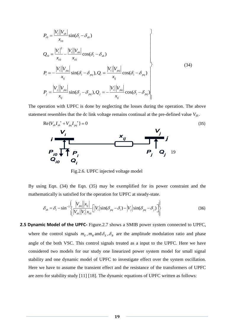
19

0

0

2

0

0 0

sin( )

cos( )

sin( ), cos( )

sin( ), cos( )

i sh

i i sh

i

i i sh

i i sh

i i

i pq i pq

i i pq i i pq

ij ij

j pq i pq

j j pq j i pq

ij ij

V VP

x

V V VQ

x x

V V V VP Q

x x

V V V VP Q

x x

(34)

The operation with UPFC is done by neglecting the losses during the operation. The above

statement resembles that the dc link voltage remains continual at the pre-defined value Vdc.

Re{ } 0sh sh pq pqV I V I (35)

19

Fig.2.6. UPFC injected voltage model

By using Eqn. (34) the Eqn. (35) may be exemplified for its power constraint and the

mathematically is satisfied for the operation for UPFC at steady-state.

1

0

sin sin( ) sin( )pq ij

sh i i pq i j pq j

sh i i

V xV V

V V x

(36)

2.5 Dynamic Model of the UPFC- Figure.2.7 shows a SMIB power system connected to UPFC,

where the control signals Em , Bm and E , B are the amplitude modulation ratio and phase

angle of the both VSC. This control signals treated as a input to the UPFC. Here we have

considered two models for our study one linearized power system model for small signal

stability and one dynamic model of UPFC to investigate effect over the system oscillation.

Here we have to assume the transient effect and the resistance of the transformers of UPFC

are zero for stability study [11] [18]. The dynamic equations of UPFC written as follows:

20

0

1 2

34

0

6

00 0 0

0

10

10

0 0 0 0

pd

qd dc

qd do doq do

qeqe A s A A vd

A A A A

pe p e

KK KD

M M M M

K KK VE

T T TE TE

E K K K K K K

T T T T

K K

M M

0 0 0 0

pb p bE

E

qe q e qb q b

B

d d d d

B

A ve A v e A vb A v b

A A A A

K Km

M M

K K K Km

T T T T

K K K K K K K K

T T T T

cos( )

0 2

0 sin( )

2

cos( )

0 2

0 sin( )

2

E dc E

Etd EdE

Etq EqE E dc E

B dc B

Btd BdB

Btq BqB B dc B

m vv iX

v iX m v

m vv iX

v iX m v

(37)

3 3[cos( ) sin( )] [cos( ) sin( )]

4 4

Ed Bddc E BE E B B

Eq Bqdc dc

i idv m m

i idt C C

By combining equation (37) and machine dynamic equation of the UPFC, we can develop

complete dynamic model of the SMIB system connected with UPFC as follows:

0

0

( ) / , ( ) / (1 )

, ( ) / 2

q q qe d qe A to t A

m e

E E E T E K V V sT

P P D H

(38)

By merging and linearizing Equations (37) and (38), the power system with UPFC state

equations as follows:

(39)

(39)

Where Em , Bm , E and B be the deviance of control input signals of the UPFC

21

'

qE

1Ms D

0ωs

2K

4K

5K

6K

3

'

3 01 d

K

sK T 1

KasTa

'

fdE

1K

f

vKqKpK

dc E E B B

pd pe p e pb p b

p

T

qd qe q e qb q b

q

do do do do do

T

A vd A ve A v e A vb A v bv

A A A A A

f v m m

K K K K KK

M M M M M

K K K K KK

T T T T T

K K K K K K K K K KK

T T T T T

Fig.2.7. A UPFC installed in SMIB system.

This linearize model (Figure 2.8.), which is then established by increasing the nonlinear

differential equations about a normal operational point. Here the performance of the SMIB

system has been studied under different disturbances i.e. frequent load changes, the constants

of the UPFC are calculated as:

(40)

Fig.2.8. H-P model of SMIB system with UPFC

22

2.6 Power System Stabilizer-An economic and satisfactory solution to the unstable

oscillations a power system produces is to provide additional damping (to rotor windings) for

the generator rotor. This is done via Conventional PSS which gives additional controllers to

the excitation system [7]. The input Vs to the exciter (Figure 2) is, as seen in Figure 2.9 the

output from the Power System Stabilizer whose input signal originates from rotor velocity (or

frequency). Conventional Power System Stabilizers are modeled in the following manner:

The Power System Stabilizer implemented consists, as shown in Figure 2.9, of three main

functional blocks:

-Lag Compensator

Fig 2.9. Conventional PSS

The Gain of PSS:

The Gain is simply the proportional gain of the PSS.

The Washout Circuit:

At the output of the PSS there is a steady state bias which modifies the generator terminal

voltage; this is eliminated through the use of a Washout Circuit [5]. In the input signal the

Power System Stabilizer acts upon only the transient variations. It doesn’t however take any

action when DC offsets in the signal are present. By subtracting the low frequency

components from the input signal (through the use of a low-pass filter essentially) the DC

offset present in the signal can be removed. Hence it can be said that Washout Circuits are

essentially High-Pass filters which pass all frequencies that are of interest. It is understood

that the system under investigation is of local mode nature and so the Tw value be placed in

the range of 1 and 2.

The Dynamic Compensator, Lead – Lag Compensation:

The final process contained within the Power System Stabilizer is the Dynamic Compensator.

This stage comprises of lead-lag stages and has the transfer function as shown in Figure 6.

INPUT

OUTPUT

23

The Lead-Lag stage utilizes the rotor shaft angular velocity and uses it as the inputs signal

(as mentioned previously about the Washout Circuit) [7]. The Lead-Lag time constants: T1

and T2 were allocated values such that when the PSS is included in the feedback loop the

overall closed loop of the H-P model and UPFC is stable at a set operating point. See Figure

2.10.

Tuning:

Given the above knowledge of PSS, the following values for the various parameters in

relation to it were allocated

Fig. 2.10 UPFC with Power System Stabilizer

2.7 Fuzzy Logic Controller- In order to providing stabilizer signal, the output of obtained

model reference of power system is compared with output of real power system and the error

signal is fed to a fuzzy controller [14]. The Fuzzy controller provides stabilizer signal in order

to damping system oscillations. Fig. 2.11. Present the block diagram of proposed Fuzzy logic

controller. In fact Fuzzy logic controller is one of the most effective operations of fuzzy set

theory; its key features are the use of linguistic variables relatively than numerical variables.

This control technique depends on human competency to understand the system performance

and is based on quality control rules. Fuzzy logic provides a simple technique to reach at a

definite conclusion created upon ambiguous, uncertain, inaccurate, noisy, or lost input

information. FLC work on the principle of simple understanding of the system behavior of a

person and simple rule based “If x and y then z”, this rule base again defined by some

membership function of FLC with proper argument to enhance the system performance [16]

[17] [18]. The UPFC with Fuzzy controller is shown in the figure 2.12. Inaccurate, noisy, or

lost input information. FLC work on the principle of simple understanding of the system

behavior of a person and simple rule based “If x and y then z”, this rule base again defined by

24

some membership function of FLC with proper argument to enhance the system performance

[16] [17] [18]. The UPFC with Fuzzy controller is shown in the figure 2.12.

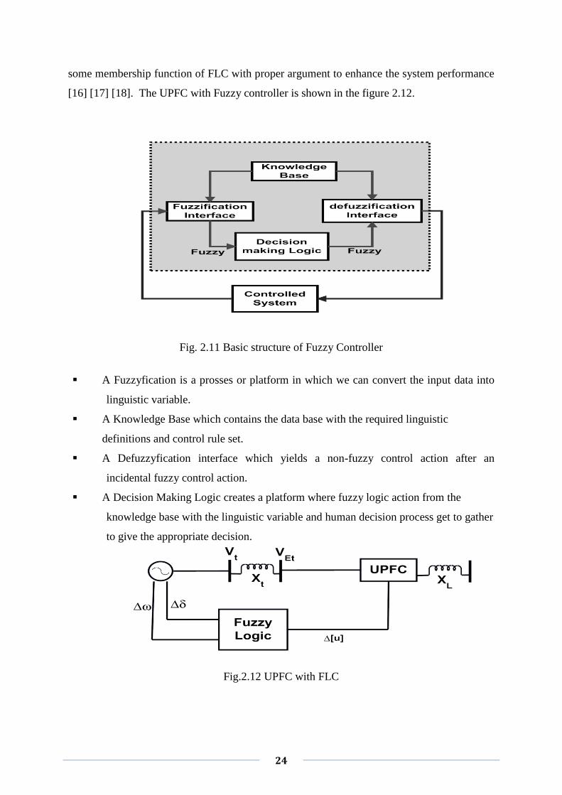
Fig. 2.11 Basic structure of Fuzzy Controller

A Fuzzyfication is a prosses or platform in which we can convert the input data into

linguistic variable.

A Knowledge Base which contains the data base with the required linguistic

definitions and control rule set.

A Defuzzyfication interface which yields a non-fuzzy control action after an

incidental fuzzy control action.

A Decision Making Logic creates a platform where fuzzy logic action from the

knowledge base with the linguistic variable and human decision process get to gather

to give the appropriate decision.

Fig.2.12 UPFC with FLC

25

FLC parameters: -

FLC structure:

The Rules used in this controller are chosen as follows:

If ∆ω is P and ∆δ is P then ∆[u] is P.

If ∆ω is P and ∆δ is N then ∆[u] is Z.

If ∆ω is N and ∆δ is P then ∆[u] is Z.

If ∆ω is N and ∆δ is N then ∆[u] is N.

Input and output membership functions:

Input Membership Function

Ouput Membership Function

Input Membership Function

2.7.1 Hybrid Fuzzy Logic Controller-It is a combination of conventional FLC and

conventional PI controller. The internal arrangement of the hybrid fuzzy damping controller

26

∆U

dv/dt

Derivative

Fuzzy Logic Controller

Kp

Ki

+

+

+

+

KDcm1

∆δ,∆ω K-K-

displayed in the Fig.2.13.The membership functions, the rule base used here is same as of

conventional FLC.

Fig. 2.13 Hybrid fuzzy damping controller structure

2.8 SIMULATION RESULTS and DISCUSSION

The K-constants of SMIB system are calculated under the nominal condition with and

without UPFC:

1 2 3 4 5 61.1253, 0.29611, 0.46154, 0.20755, 0.01055, 0.49647

0.53564, 2.1595, 0.49398pe qe ve

K K K K K K

K K K

Operating condition:

1.0 . , 1.0 . , 50t bV p u V p u f Hz

Parameter of DC link capacitor:

2, 1dc dcV C

Constants for PSS Controller [17]:

1 24.33, 2, 0.45012, 0.1133,max 0.15,min 0.015STAB wK T T T

Excitation System:

0.05, 50A AT K

Power System Data:

0 7.76, 1.0, 0.6, 0.3, 4, 2d d q dT X X X H M H .

Hybrid Fuzzy Logic Data [19]:

Kp=5, Ki=5, KD=1

The output of the simulation model is taken as speed deviation (∆ω) angle deviation (∆δ). So,

the following response is performed for speed deviation (∆ω) and angle deviation (∆δ)

against time from simulation model using SMIB system. The simulation process is carries for

duration of 10 seconds [11].

27

0 5 10 15-0.04

-0.02

0

0.02

0.04

Time (seconds)

Spee

d

Variation of Speed Vs Time

Speed

0 5 10 150

0.5

1

1.5

2

2.5

Time (seconds)

Ang

le

Variation of Angle Vs Time

Angle

SIMULATION RESULTS:

Effect Step change in mechanical Power input on Power System Oscillations without

UPFC. From viewing response of the system in figure 2.14 we have, the variation in

speed and angle is oscillatory in nature. Due to formation of these oscillations the

system is unstable. To improve the system performance and getting the stable position

we have to eliminate these oscillations. To eliminate these oscillations we install

UPFC with this SMIB system.

Fig. 2.14 Response of SMIB system without UPFC

Effect Step change in mechanical Power input on Power System Oscillations with

UPFC without external controlling signal is shown in the Figure 2.15. By calculating

constants for FACTS device (UPFC) i.e. Kp, Kq and Kv. We can see the effect of

28

0 5 10 150

0.5

1

1.5

2Variation of Angle Vs Time

Time (seconds)

Ang

le

Angle

0 5 10 15-0.02

-0.01

0

0.01

0.02

Time (seconds)

Spee

d

Variation of Speed Vs Time

Speed

UPFC on power system. As we know that, the significant control parameters of UPFC

are Em ,

Bm and B

E . By controlling these parameters we can control the magnitude

of voltage through reactive power compensation at a bus where the UPFC is installed,

also we can control the magnitude of the series injected voltage. Also we can regulate

the d.c link voltage.

Fig. 2.15 Response of SMIB system with UPFC

Effect Step change in mechanical Power input on Power System Oscillations with UPFC

and external controlling signal from power system stabilizer is shown in the Figure 2.16.

As we can see that using UPFC the oscillation of SMIB is reduced. But still the system is

having oscillations which should be damped. So we install a damping controller on

UPFC.

29

0 5 10 15-0.02

-0.01

0

0.01

0.02

Time (seconds)

Spee

dVariation Speed Vs Time

Speed

0 5 10 150

0.5

1

1.5

2

Time (seconds)

Ang

le

Variation Angle Vs Time

Angle

Fig. 2.16 Response of SMIB system with UPFC and Power System Stabilizer

Effect in mechanical power input to the excitation on System Oscillations with UPFC and

external controlling signal from Conventional -FLC is shown in the Figure 2.17. In this

sub section we install a fuzzy damping controller for UPFC.

30

0 5 10 150

0.5

1

1.5

2

Time (seconds)

Ang

le

Variation of Angle Vs Time

Angle

0 5 10 15-0.02

-0.01

0

0.01

0.02

Time (seconds)

Spee

dVariation of Speed Vs Time

Speed

Fig. 2.17 Response of SMIB system with UPFC and Conventional Fuzzy Logic Controller

Effect in mechanical power input to the excitation on System Oscillations with UPFC and

external controlling signal from Hybrid -FLC is shown in the Figure 2.18.

31

Fig. 2.18 Response of SMIB system with UPFC and Hybrid Fuzzy Logic Controller

Comparison study of the impact of all controllers to the UPFC for controlling the

effect of step changing on mechanical power input to the SMIB system is shown in

the figure 2.19.

0 2 4 6 8 100

0.1

0.2

0.3

0.4variation of Angle Vs Time

Tme(second)

An

gle

32

0 1 2 3 4 5 6 7 8 9 10-0.04

-0.02

0

0.02

0.04Variation of Speed Vs Time

Time(second)

Sp

eed

Without controller With UPFC With PSS-UPFC With Fuzzy logic contoller-UPFC With Hybrid Fuzzy logic contoller-UPFC

0 1 2 3 4 5 6 7 8 9 10-1

0

1

2

3

Time(second)

An

gle

Variation of Angle Vs Time

Without Controller With UPFC With PSS-UPFC With Fuzzy Logic Controller-UPFC With Hybrid Fuzzy Logic Contoller-UPFC

Fig. 2.19 Comparison of Response of SMIB system without and with UPFC with

various controllers

33

Results Comparison:

CONTROLLERS

WITHOUT

UPFC

WITH

UPFC

UPFC

WITH

PSS

UPFC WITH

CONVENTIONAL

FUZZY LOGIC

CONTROLLER

UPFC WITH

HYBRID

FUZZY LOGIC

CONTROLLER

Settling

Time(speed) infinite 50 sec 15 sec 7.1 sec 3.3 sec

Settling

Time(angle) infinite 50 sec 15 sec 7.2 sec 3 sec

Table.1 Comparison of Response of SMIB system without and with UPFC with various

controllers

DISCUSSION- From the above study with SMIB system connected to UPFC, PSS and also

with FLC, simulation experiments and simulation results it is concluded that we can

effectively damp out the low frequency oscillations by using Fuzzy and Hybrid Fuzzy logic

controllers with only 7.2s and 3s, hence the stability of the system increases.

34

CHAPTER 3

.

35

CHAPTER 3

3.1 Introduction- The swift evolution of Power electronic sector gives an new idea and also

empower the field of power system in many manner by developing new power electronics

equipment’s under the name of FACTS technology and is very much popular in last few

decades. UPFC is used as most versatile and effective among all FACTS controllers for

incising the stability of a system as well as control the power flow in the line [20]. This

chapter also briefing the linear model of UPFC connected with the line and externally

controlled by the signal from the proposed power flow controller to damp out the system

oscillation with stability study with occurrence of fault. The proposed controller consist of

Power oscillation damping controller and Proportional Integral Differential controller(POD

& PID).The PID controller parameter has been optimized by Ziegler-Nichols tuning

method. The simulation model is tested for both S-L-G and 3-ø faults. A power system is

designed and examined by using phasor simulated process and the system is tested in three

stages; without having UPFC, with UPFC but not having any external signal, power system

having new proposed controller. It is seen that without the controller the all system

parameters goes to unstable. When UPFC is connected in the system, it becomes stable.

Again, when the UPFC is externally controlled by the proposed controller, the power

system parameters (P, Q, and V) become stable very rapidly. It has been observed that

UPFC rating is only 15 MVA with controller and 100 MVA without controllers. Therefore,

UPFC is very effective to enhance the power system stability in good manner and also

damp the power system oscillation.

3.2 CONTROL CONCEPT OF UPFC- The classical connection of UPFC with transmission

line shown on the figure.3.1. The UPFC uses a two back-to back VSCs, operated from a

common dc link. The converter 2 injects the controllable voltage both magnitude and phase

angle to the connected line via series transformer. The converter 1 called STATCOM

supplies or absorbed the real power demand by the converter 2 via dc link which then

support the real power exchange between them. Conceptually the UPFC can automatically

control all the system parameter that affect the power flow in a line, namely, voltage,

impedance, and phase angle, hence, the name suggested “unified”[20]. The UPFC provides

complete control over power flow in the line. A circuit equivalent diagram of the UPFC is

show in the fig.3.2.

36

lI

vRV vR

vRZ

cRZmI

vRI

cRV cR

lV lmlV m

1I

0}Re{

mcRvRvR IVIV

Fig.3.1. Connection diagram of UPFC with transmission line

3.3. UPFC BASED CONTROL SYSTEM- There is two modes of operation

1. PFC mode or automatic mode and

2. Manual voltage injection made

In the power control mode the comparison between the actual and reference values of the

active and reactive power is made to produce an error P and Q. This error P and Q again

synthesize by two voltage regulator and the VSC to compute the Vd and Vq. component

(Vd and Vq are the direct and quadrature axis component with the voltage V1 to control the

power flow in the line). In manual voltage injection mode the use of voltage regulator is

absent. The voltage of the converter is synthesized by the injected voltage Vdref and Vqref

[20]. Fig.3.3 shows the block diagram of series converter

Fig.3.2. A general circuit equivalent of UPFC

37

Fig.3.3. UPFC based control system

3.4. POWER SYSTEM MODEL WITH UPFC- Here model of a modest power system

comprising of two-hydraulic power plants connected to a power grid is illustrated [21]. The

whole Simulink model shown in figure.3.4. A UPFC is connected to regulate the power flow

in a 500/230 kV transmission line. The power system used under the study is assembled in a

loop arrangement, and it combination of five buses (B1, B2, B3, B4, B5).Three lines L1 to L3

are connected to make a ring system. Each plant having their own PSS, excitation system,

speed regulators. The fig.3.4 shows the single line diagram of the two- machine system

connected with UPFC. The UPFC is connected to the bus 3 via line 1-2 to control both the

powers in the system also it control the voltage at the bus B_UPFC using two VSCs via dc

link capacitor and the coupling reactors and the through transformers. The total generating

capacity of 1500 MW and load connected are 1500 MVA, 500 KV, and 200 MW.

38

Fig.3.4 Single line diagram of two-machine power system with UPFC controller

3.5. DESIGN OF POWER FLOW CONTROLLER

The projected power flow controller consist of two different controllers, A. PID controller

which is tuned by Ziegler-Nichols tuning method, B. POD controller.

3.5.1. PID Controller Tuning Process:

Input to the PID controller is the machine angular speed deviation and gives the output as an

error signal. The PID tuning is done to selecting the proper controller parameter to meet the

desire performance at particular condition. Most PID controllers are adjusted on-site, many

types of tuning rules have been proposed in different literatures [22] [23]. The dynamic

equation of PID control is given as:

∫

In Laplace Form,

(

)

39

Block diagram of PID controller Parameters is shown in the figure.3.5, for selecting the

proper controller parameter, Ziegler-Nichols PID tuning method which is being used for the

known system dynamics of the given plant is used. The parameter is selected as τi=∞,

τd=0.By means of the proportional controller action the Kp is increased from 0 to critical

value Kcr which is shown in figure.3.6., Fig.3.7 shows the output of the sustained oscillation.

Fig.3.5 Block diagram of PID controller Parameters

Fig.3.6 Proportional action of PID controller

Fig.3.7 Calculation of sustained oscillation (Pcr)

Fig.3.8 PID controller with tuning parameters

40

Thus experimentally the critical gain Kcr & its corresponding critical time period Pcr are

determined. Then according to Ziegler and Nichols the value of the parameter Kp, τi, τd

must set according to the subsequent formula.

Kp=0.6Kcr, τi=0.5Pcr, τd=0.125Pcr

Using this tuning method for PID controller, the result which is obtained is given by,

(

)

Thus the PID controller has a pole at origin and two zeros at S= -4/Pcr. It is found that, Pcr

=0.2s & Kcr =200 from figure 3.5. Block diagram of PID controller with tuning parameter

shown in the figure.3.8. By taking the input as machines angular speed deviation dω1 and

dω2 it generates an output error signal dω, which is shown in the figure.3.9.

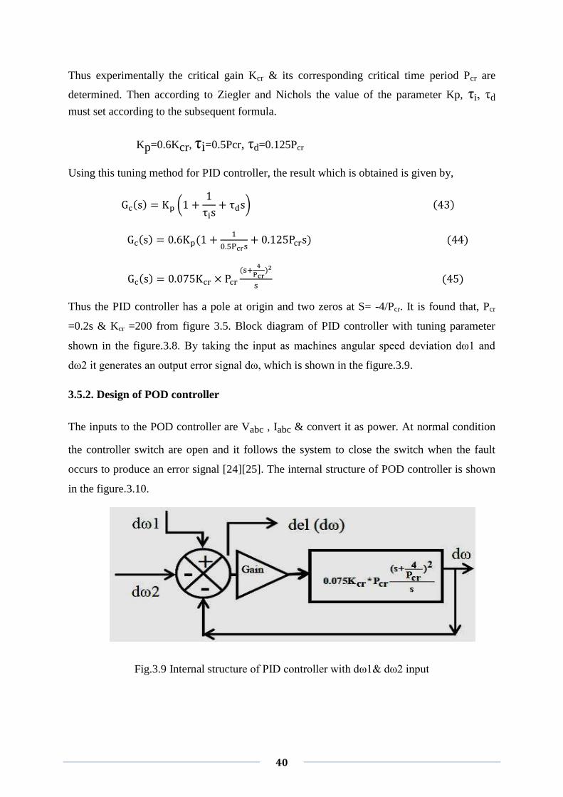
3.5.2. Design of POD controller

The inputs to the POD controller are Vabc , Iabc & convert it as power. At normal condition

the controller switch are open and it follows the system to close the switch when the fault

occurs to produce an error signal [24][25]. The internal structure of POD controller is shown

in the figure.3.10.

Fig.3.9 Internal structure of PID controller with dω1& dω2 input

41

Fig.3.10 Internal structure of POD controller

Fig.3.11 Complete model of Power Flow Controller

Finally two error signals one from PID and other from POD has been added to form Power

System Controller to give the reference voltage signal Vqref. This output is used as a

reference signal and again given to the UPFC when it operates in manual voltage injection

mode for improving the stability and damp out the oscillation. The complete internal structure

of power system controller is shown in the figure.3.11.

3.6 SIMULATION RESULTS AND DISCUSSION

The simulation is carried out for two different types of fault condition.

Case A. S-L-G fault

Case B. 3-ø fault

Case A.1: S-L-G fault (without UPFC)When S-L-G fault happened at 0.1s and the fault

breaker unlocked at 0.2s (3-phase 4-cycle fault), as there is no UPFC connected the whole

system voltage and power turn out to be unstable. The responses of the system are shown in

fig.3.12 andfig3.13.

42

0 1 2 3 4 5 60

0.25

0.5

1

1.25

1.5

2

Time(sec)

Bus

Vol

tage

(p.u

)

0 1 2 3 4 5 6-2000

-1000

0

1000

2000

Time(sec)

Bus

Pow

er(M

W)

CaseA.2: S-L-G fault (UPFC without power flow controller)

If UPFC is connected, the responses of the system are shown in fig.3.14 and fig.3.15.

Case B.1: 3-ø (without UPFC)

Throughout 3-Phase faults, if UPFC is not connected, then again system voltage and

power going to be unstable. The simulation results are shown in figure.3.16 and

figure.3.17.

Case B.2: 3-ø fault (UPFC without power flow controller)

During Three-Phase faults, If UPFC is connected to the system, the simulation results are

shown in the figure.3.18 and figure.3.19.

Case A.3: S-L-G fault (UPFC with power flow controller)

If UPFC with PFC is connected to the system, the simulation results are shown in fig.3.20

and fig.3.21.

Case B.3: 3-ø fault (UPFC with power flow controller)

During Three-Phase faults, If UPFC is connected to the system, the simulation results are

shown in the figure.3.22 and figure.3.23.

Fig.3.12 Bus voltage (B1) in p.u. without UPFC

Fig.3.13 Bus power (B1) in MW without UPFC

43

0 0.2 0.4 0.6 0.8 1 1.2 1.4 1.5

0.6

0.7

0.8

0.9

1

1.1

1.2

1.3

1.4

Time(sec)

Bus

Vol

tage

(p.u

)

Va

Vb

Vc

0 0.2 0.4 0.6 0.8 1 1.2 1.4 1.6

0

500

1000

1500

2000

2500

Time(sec)

Bus

Pow

er(M

W)

Pa(MW)

Pb(MW)

Pc(MW)

0 0.2 0.4 0.6 0.8 1 1.2 1.4 1.6 1.8 20

0.5

1

1.5

Time(sec)

Bus

Vol

tage

(p.u

)

Fig.3.14 Bus voltage in p.u. (UPFC without power flow controller)

Fig.3.15 Bus power in MW (UPFC without power flow controller)

Fig.3.16 Bus voltage (B1) in p.u. without UPFC

44

0 0.5 1 1.5 2-2000

-1000

0

1000

2000

Time(sec)

Bu

s P

ow

er(M

W)

power

0 0.2 0.4 0.6 0.8 1 1.2 1.4 1.5

0.6

0.7

0.8

0.9

1

1.1

1.2

1.3

1.4

Time(sec)

Bus

Vol

tage

(p.u

)

Va

Vb

Vc

Fig.3.17 Bus power (B1) in MW without UPFC

Fig.3.18 Bus voltage in p.u. (UPFC without power flow controller)

Fig.3.19 Bus power in MW (UPFC without power flow controller)

0 0.1 0.2 0.4 0.6 0.8 1 1.2 1.4 1.6 1.8 2-1000

0

1000

2000

3000

Time(sec)

Bus

Pow

er(M

W)

Pa(MW)

Pb(MW)

Pc(MW)

45

0 0.1 0.2 0.3 0.4 0.5 0.6 0.70.4

0.6

0.8

1

1.2

1.4

Time(sec)

Bus

Vol

tage

(p.u

)

Vc

Va

Vb

0 0.1 0.2 0.3 0.4 0.50

0.5

1

1.5

2

Time(sec)

Bus

Vol

tage

(p.u

)

Vc

Vb

Va

0 0.2 0.4 0.6 0.8 1 1.2

0

500

1000

1500

2000

2500

Time(sec)

Bus

Pow

er(M

W)

Pa(MW)

Pb(MW)

Pc(MW)

Fig.3.20 Bus voltage in p.u. (UPFC with power system controller)

Fig.3.21 Bus power in MW (UPFC with power system controller)

Fig.3.22 Bus voltage in p.u. (UPFC with power flow controller)

46

0 0.2 0.4 0.6 0.8 1 1.2 1.4-3000

-2000

-1000

0

1000

2000

3000

Time(sec)

Bus

Pow

er(M

W)

Pa(MW)

Pc(MW)

Pb(MW)

Fig.3.23 Bus power in MW (UPFC with power flow controller)

The performance of UPFC with Power Flow Controller having same 500KV

transmission line is summarized in table 1. Below.

Table.2 The performance of UPFC with PFC having same 500KV transmission line

DISCUSSION: - The above simulation results gives an idea about that UPFC not only

significantly increases transient stability limits but also compensates the power system

oscillations during both single phase and three phase faults. The UPFC with power flow

controller very much effective to control the both active and reactive power flow of power system

by injecting suitable reactive power during fault condition and damp the oscillation for active

power in just 1.25s for single phase and 1.4s for three phase faults and for voltage it is 0.6s single

phase and 0.3s for three phase.. We also conclude that if the fault clearing time is less, more

stability improvement. On the other hand less transient stability improvement occurs if fault

clearing time is more.

SETTLING TIME

1-Phase Fault 3-Phase Fault

Status UPFC Voltage Active Power Voltage Active Power

No UPFC NO

UPFC 100MVA 1.5s 1.6s 1.5s 2.1s

UPFC+PFC 15MVA 0.6s 1.25s 0.3s 1.4s

47

CHAPTER 4

CONCLUSION AND FUTURE SCOPE

48

CHAPTER 4

4.1 CONCLUSION-In the chapter 2, a brief discussion is made about the LFO and small signal

stability of a system. A linearize Haffron-Philips model is considered and a dynamic behavior

of the system was examined by using different controllers like UPFC with power system

stabilizer, conventional Fuzzy logic controller, Hybrid fuzzy logic controller..etc. to the small

change in excitation and mechanical input. From the figure it is observed, that the planned

Hybrid fuzzy logic UPFC controllers significantly damp power system oscillations

effectively compared to the conventional Fuzzy logic UPFC. In chapter 3, the whole system

presents the effectiveness and stability response of the UPFC without and with power flow

controller on the dynamic behavior of the power system with external fault, real & reactive

power flow, voltage level for different type of fault (single and three phase faults) conditions.

If Power Flow Controller is connected then lesser rating of UPFC becomes sufficient for

stabilization of the system oscillation at very shortest interval of time for both the steady and

dynamic conditions.. This power flow controller can use with any FACTS devices for any

type of system like single or multi machine system to enhance the stability of the system with

damping the oscillation .

4.2 FUTURE SCOPE- These proposed controller can applied to any other FACTS devices with

tuning algorithm i.e. ANN, Fuzzy logic, Genetic algorithm. In future a Fuzzy logic based

POD controller will be designed to control the UPFC for power system oscillations. We can

also enhance our projects from SMIB system to multi machine system for small signal

analysis.

ix

REFERENCES

[1]. P.Kundur, “Power System Stability and Control”, McGraw-Hill, 1999.

[2]. Hingorani NG, Gyugyi L (2000). Understanding FACTS, IEEE Press, pp., 323-387.

[3]. T. J. E. Miller, Reactive power control in electric systems, Wiley Interscience

Publication, 1982.

[4]. M.H. Haque,“Damping improvement using FACTS devices”. Electrical Power Syst. Res.

Volume 76, Issues 9-10, June 2006.

[5]. M. Zarghami, M. L. Crow, J. Sarangapani, Y.Liu and S. Atcitty. “A novel approach to

interarea oscillation damping by unified power flow controller utilizing ultracapacitors”,

IEEE Transactions on Power Systems, vol. 25, no.1, pp. 404-412, 2010.

[6]. H. Saadat, “Power System Analysis”, McGraw-Hill, 2002.

[7]. A.Chakrabarti, S.Halder, “Power System Analysis and Control”, Third Edition, Chapter

15,Page no 744 -830.

[8]. N.G. Hingorani and L. Gyugyi, “Understanding FACTS: concepts and technology of

flexible ac transmission systems”, IEEE Press, NY, 1999.

[9]. Y.H.Song, A.T. Johns (Eds), “Flexible A.C. Trans-mission Systems (FACTS)”,IET,

1999, Chapter 7, Pages 1-72.

[10]. Z. Huaang, Y.X. Ni, C. M. She, F. F. Wu, S. Chen, and B.Zhang, “Application of Unified

Power Flaw controller in interconnected Power Systems modeling, interface, control,

strategy, and case study”, IEEE Trans. On Power Systems. Vol.15, No.2, pp. 817-824,

May 2000.

[11]. H. F. Wang, F. J. Swift, “A Unified Model for the Analysis of FACTS Devices in

Damping Power System Oscillations Part I: Single-machine Infinite-bus Power Systems,”

IEEE Transactions on Power Delivery, Vol. 12, No. 2, April, 1997, pp. 941-946.

[12]. H. F. Wang, F. J. Swift, “A Unified Model for the Analysis of FACTS Devices in

Damping Power System Oscillations Part II: Multi-machine Power Systems,” IEEE

Transactions on Power Delivery, Vol. 13, No. 4, October, 1998, pp. 1355-1362.

[13]. HaiFeng Wang, Member, IEEE, “A Unified Model for the Analysis of FACTS Devices

in Damping Power System Oscillations”—Part III: Unified Power Flow Controller, IEEE

Transactions on Power Delivery, vol. 15, no. 3, july 2000.

[14]. A. A. Eldamaty S. O. Faried S. Aboreshaid, “damping power system oscillations

using a fuzzy logic based unified power flow controller”,IEEE conference,

CCECE/CCGEI, Saskatoon, May 2005,0-7803-8886-0/05/$20.00@2005 IEEE.

x

[15]. N.Tambey, M.L.Kothari, “Damping of Power System Oscillations with Unified

Power Flow Controller”, IEE Procdceding-Gener.Trans.Distri., Vol.150, No 2, March

2003.

[16]. R.H.Adware, P.P.Jagtap and J.B.Helonde, “Power System Oscillations Damping using

UPFC Damping Controller”, IEEE conference, Third International Conference on

Emerging Trends in Engineering and Technology, 2010.

[17]. N. Bigdeli, E. Ghanbaryan, K. Afshar., “low frequency oscillations suppression via

cpso based damping controller, “journal of operation and automation in power

engineering”, vol. 1, no. 1, March 2013.

[18]. R.Manrai, Rintu Khanna, B.Singh, P Manrai, “Power system Stability using Fuzzy

Logic based Unified Power Flow Controller in SMIB Power System”,IEEE

Conference,978-1-4673-0449-8/12/$31.00©2012 IEEE.

[19]. Ravindra Sangu, Veera Reddy.V.C, Sivanagaraju. “Damping power system

oscillations by sssc equipped with a hybrid damping controller”, IJAREEIE, Vol. 2,

Issue 7, July 2013.

[20]. S. Tiwari, R. Naresh, R. Jha, “Neural network predictive control Predictive control of

UPFC for improving transient stability Performance of power system”, Applied Soft

Computing, Volume 11, Issue 8, December 2011, Pages 4581-4590,ISSN 1568- 4946.

[21]. Gyugyi, L. "Unified power-flow control concept for Flexible AC Transmission Systems,"

Generation, Transmission and Distribution, IEEE Proceedings, vol.139, no.4, pp.323-331,

Jul 1992.

[22]. K. Ogata, Modern Control Engineering, Fourth Edition, Prince Hall, 2002, Chapter, 10.

[23]. Md.Habibur Rahman, Md. Harun-Or-Rashid, Sohel Hossain, “stability improvement

of power system by using PSC controlled UPFC”, IJSETR, Volume 2, Issue 1, January

2013.

[24]. Meysam Eghtedari, Reza Hemmati, and Sayed Mojtaba Shirvani Boroujeni,” Multi

objective control of UPFC using PID type Controllers” International Journal of the

Physical Sciences Vol. 6(10), pp. 2363-2371, 18 May, 2011.

[25]. S.N. Dhurvey and V.K. Chandrakar: “Performance Comparison of UPFC in Coordination

with Optimized POD and PSS On Damping of Power System Oscillations”, WSEAS

Transactions on Power Systems, Issue 5, Vol. 3, pp. 287-299, May 2008.

xi

PUBLICATION

[1] Sudhansu Kumar Samal, P.C.Panda, “Damping of Power System Oscillations by Using

Unified Power Flow Controller with POD and PID Controllers”, IEEE Conference

(ICCPCT), 2014, .978-1-4799-2395-3/14/$31.00 ©2014 IEEE.