University of New England

School of Economics

AN ANALYSIS OF STRESS TESTING FOR ASIAN STOCK PORTFOLIOS

by

SHEN WANG, CHONG MUN HO AND BRIAN DOLLERY

No. 2003-3

Working Paper Series in Economics

ISSN 1442 2980

http://www.une.edu.au/febl/EconStud/wps.htm

Copyright © 2003 by Shen Wang, Chong Mun Ho and Brian Dollery. All rights reserved. Readers may make verbatim copies of this document for non-commercial purposes by any means, provided this copyright notice appears on all such copies. ISBN 1 86389 830 1

2

AN ANALYSIS OF STRESS TESTING FOR ASIAN STOCK PORTFOLIOS

SHEN WANG, CHONG MUN HO AND BRIAN DOLLERY∗∗

Abstract

While extreme asset price movements are a common feature of the global financial system, recent financial crises have witnessed an increase in the use of serious stress testing in risk management. This paper examines the performance of a bivariate normal distribution model and a bivariate mixture of two normal distributions model in the institutional context of five Asian stock markets, namely Bangkok, Hong Kong, Seoul, Taipei and Tokyo. To assess the performance of the two models, the data from the five stock markets for the period 4 January 1990 to 28 February 1998 are employed. The results show that the bivariate normal distribution model outperforms the bivariate mixture of two normal distributions model. This seems to suggest that the latter model can more precisely capture the fat-tailed property of left and right tails in return distributions.

Key Words: Stress Testing; Bivariate Normal Distribution Model; Bivariate Mixture of Two Normal Distributions Model; Backtesting.

∗∗ Shen Wang is a Senior Research Fellow in Education and Development Department Securities and Futures Institute, Taiwan. Chong Mun Ho School is at the Science & Technology Universiti Malaysia Sabah, Kota Kinabalu, Sabah, MALAYSIA and Brian Dollery is Professor in the School of Economics, University of New England. Contact information: School of Economics, University of New England, Armidale, NSW 2351, Australia. Email: bdollery@metz.une.edu.au.

3

An Analysis of Stress Testing for Asian Stock Portfolios

1. Introduction

The Asian financial crisis in 1997 has witnessed a renewed interest amongst

scholars and practitioners alike in stress testing as an important risk management tool

for asset portfolio assessment. As defined by International Organization of Securities

Commissions (IOSCO 1995), stress tests apply particular ‘worst-case’ assumptions to

a given portfolio to determine the effects of specific and severe adverse market

movements on financial institutions, and to identify what potential losses would arise

if the envisaged ‘worst-case’ scenario eventuated. The Basle Capital Accords of the

Bank for International Settlement (BIS 1995, 1996) stipulate that financial institutions

should use Value-at-Risk (VaR) models to calculate the potential risk on capital. It

also requires these institutions should also perform stress tests as an additional

dimension of risk management. Moreover, RiskMetrics (1999) has indicated that,

employed in tandem, VaR and stress tests provide a ‘boarder picture of risk’.

The BIS (1996) stresses two important complementary features of stress testing.

Thus, while its quantitative characteristics enable analysts to identify plausible stress

scenarios to which financial institutions could be exposed, its qualitative

characteristics allow managers to evaluate the capacity of a financial institution to

absorb capital large capital losses. Managers are thus able to identify those measures a

financial institution can take to reduce its risk and to conserve its capital. The 1999

4

IOSCO report also underlines the unique functions of stress testing. This report argues

that stress testing should be performed regardless of whether the institution uses VaR

models, since stress tests quantify the extreme risks that may threaten the firm.

Accordingly, regulatory advice from international supervisory organizations, as well

as potentially serious losses contingent upon financial crises, have induced financial

institutions to disclose both the methodology and/or the results of stress testing in

their annual reports. Leading examples include Citibank, Chase, United Bank of

Switzerland, Deutsche Bank and the Canadian Imperial Bank of Commerce1.

The need for stress testing is well documented. For example, Best (1998, 1999)

argues that the primary purpose of risk management is to prevent a financial

institution from suffering catastrophic losses, defined either as total institutional

failure or as severe material damage to its competitive position. In procedural terms,

the risk management function should report the estimated stress losses to senior

management. This information can then be employed to design the long-term risk

profile and determine the stress limits. Sound contingency plans should only be

developed after such limits have been decided. However, traditional stress testing

methods ignore the assessments of probabilities of extreme events, and thus their

results may be misleading for risk management in financial firms. Furthermore, the

1 Please refer to the 1998 annual reports of these banks.

5

BIS (1999) holds that the performance of stress test systems solely based on historical

or hypothetical scenario analysis is not satisfactory.

In this paper, the specifications for stress testing are compared for Kupiec’s

(1998) multivariate normal distribution model and Kim and Finger’s (1999) bivariate

mixture of two normal distributions model. To assess the comparative performance of

these two models, data from the Tokyo, Seoul, Bangkok, Hong Kong and Taipei stock

markets are used for the period 4 January 1990 to 28 February 1998.

The paper itself is divided into three main sections. In section II, we specify and

compare Kupiec’s (1998) multivariate normal distribution model and Kim and

Finger’s (1999) bivariate mixture of two normal distributions models from the

perspective of stress testing. Section III discusses the empirical application of these

models to data drawn from the five Asian stock markets. The paper ends with some

brief concluding comments in section IV.

2 Methods and Model Specifications for Stress Testing

Traditional stress testing methods are intrinsically scenario-orientated: namely,

the standard scenario approach, the historical scenario approach and the hypothetical

scenario approach. In the first place, the standard scenario approach employs a set of

conceivable situations, representing widely accepted specific extremal market

6

conditions, to evaluate the stress losses of specific portfolios. For example, the nine

specific market movements defined by the Derivatives Policy Group (1995) constitute

a standard scenario set. Breuer and Krenn (1999) point out that a regulatory

authority can easily compare the possible historical extremal loss changes of some

given institution, or alternatively, compare the differences of possible stress losses

between various institutions at a given point of time, if they are provided with

standard scenario stress test results by financial firms. However, since not all of the

portfolios held by financial institutions are the same, this method cannot evaluate

precisely the maximum losses that firms may actually face. Thus financial

institutions should develop portfolio-specific standard scenario stress testing to

comprehend the possible maximum losses contingent upon the composition of

particular portfolios.

The historical scenario approach represents a second technique that financial

institutions can use to conduct stress tests. This method employs historical market

extremal changes to assess their effects on portfolios. For instance, a stock dealer may

use information from the stock market ‘crisis’ of 1987 to measure the impact on its

current portfolios. The data requirements of this technique are straightforward.

Moreover, the method is uncontroversial: no senior management can ignore the

likelihood of such scenarios. However, it may be not useful for newly developed

7

financial products for which no past data exists. Furthermore, historical extremal

scenarios may be not the possible worst-case scenarios for a given portfolio (see, for

example, Dunbar and Irving (1998), Breuer and Krenn (1999), and Blanco (1999)).

The final scenario-orientated approach is to hypothesize the worst-case

conditions for particular portfolios (Breuer and Krenn 1999). This involves designing

the scenarios by specifying possible extremal changes in risk factors, volatilities,

correlations, etc., and then assessing the value changes of portfolios from these

hypothetical scenarios. This method emphasizes the quality of risk measures (i.e.,

whether the scenario in question is possible or probable) and is thus dependent on the

value judgments of risk analysts. However, this method may encounter the problem of

‘risk ignorance’ (Kimball 2000): Risk managers may overlook some important risk

factors that can have a great influence on portfolios.

While the three basic methods described above all have strengths and

weaknesses, they share the common problem of assigning probabilities to specific

stress scenarios. Although both Breuer and Krenn (1999) and Best (1998) contend that

this problem is essentially trivial, it has been argued elsewhere that the probabilities of

particular market conditions provide vital information for risk management (Wang et

al. 2001). Indeed, some recent studies have tried to estimate stress losses with

associated probabilities, including Zangari (1997), Kupiec (1998), Berkowitz (1999)

8

and Kim and Finger (1999). We now examine the Kupiec (1998) and the Kim and

Finger (1999) models in more detail.

2.1 Kupiec’s multivariate normal distribution model

A natural consideration is to extend the univariate normal distribution to a

multivariate distribution when the stress tests are conducted for a multi-asset

portfolio. However, this may result in overly complicated estimations and

computations. Kupiec (1998) has developed a simplified multivariate normal

distribution model. In this model, the stress tests can be performed using the

characteristics of conditional multivariate normal distribution in the framework

of VaR.

Assume that there are N assets in a portfolio, and that the first kN −

are non-care and the remaining k are core assets. A partitioned vector will

represent the return vector of the assets and is denoted as

=

t

tt R

RR

2

1~~

~ , where

tR1~ is a 1)( ×− kN vector, and tR2

~ is a 1×k vector. The return vector

follows a N -dimension normal distribution and is denoted

as

ΣΣ

ΣΣ

22

12

21

11

2

1

||,~

~~~

t

tNt NR

µµ

. If the stress loss of core assets is defined

as ],...,,[~2122 kt rrrRR == , then the expected stress loss of portfolio is shown as2:

2 For details, please refer to Kupiec (1998) and Appendix 1 in this paper.

9

)]([ 221

22121122 µµ −ΣΣ++ − RWRW tt , where tiW , is the investment weight vector

for kN − non-care and k core assets, 2,1=i . In the case of a two-asset

portfolio, if 1~r and 2

~r are assumed to be the returns of non-core and core

assets, and if the stress loss of core assets is defined as 22~ rr = , then the

expected stress losses of the portfolio can be shown as:

)]([ 2222

121122 µ

σσ

µ −++ rWrW tt = )]([ 22122

11122 µρ

σσ

µ −++ rWrW tt , (1)

where 12ρ is the unconditional correlation coefficient of 1~r and 2

~r .

2.2 Kim and Finger’s bivariate mixture of two normal distributions model

Kim and Finger (1999) considered the stress testing of a two-asset portfolio.

If we assume that the returns on two different assets are x and y respectively, x

is core asset and y is non-core asset, then a bivariate mixture of two normal

distributions model can be written as:

)(1Pr,||,~

)(Pr,||,~

22

2222

2222

22

2

22

21

1111

1111

21

1

12

periodhecticwobN

periodquietwobNyx

y

yxyx

yxyx

x

y

x

y

yxyx

yxyx

x

y

x

−=

=

σρσσ

ρσσσ

µµ

σρσσ

ρσσσ

µµ

,

(2)

where 1 and 2 are denoted as the ‘quiet’ and ‘hectic’ periods respectively.

In a similar vein to the Kupiec (1998) model, if the stress loss of core assets

is defined as xx ˆ= , then the expected stress losses of the portfolio can be

10

shown as:

)]ˆ([ˆ 222

222 x

y

yxyytxt xWxW µ

σσ

µ −++ = )]ˆ([ˆ 2222

22 xyx

x

yxytxt xWxW µρ

σσ

µ −++ , (3)

However, in contrast to the Kupiec (1998) model, the mean, standard

deviation and correlation coefficient parameters are estimated in the ‘hectic’

periods. To avoid complexity in estimating parameters, Kim and Finger (1999)

estimate the parameters initially by the whole sample data of x and then

weight the parameters by the conditional probabilities of x being derived from

‘hectic’ period3.

2.3 Investment strategies specifications and stress losses formula

To represent different investment strategies (such as long and short positions)

in different markets, the stress losses of two-market portfolios estimated by

these models can be classified into four main categories. The stress loss

formulae for four categories of Kupiec’s (1998) model are summarized in Table

1. Moreover, for the sake of expositional clarity, we assume that the stress

scenario for the core asset is set at 002.0=α ( 998.0=α ) only. Using the same

methodology set out in Table 1, we can also derive the stress losses for the four

categories for Kim and Finger’s (1999) model. The abbreviated formulae are

3 For details, please refer to Kim and Finger (1999) and also Appendix 2 to this paper.

11

shown in the Table 2. The stress scenario for core asset is once again calculated

at 002.0=α .

Table 1. Summary for Stress Losses Calculation in Bivariate Kupiec’s (1998) Model

Core asset Non-core asset

Formula

Long Long )()( 11211222 αα σρµσµ ZWZW +++ Long Short

)}()(|,)(|)({

1112112122

11211222

αα

αα

σρµσµσρµσµ

−− +−++++

ZWZWZWZWMin

Short Long )}()(

|,)(|)({

11211222

1112112122

αα

αα

σρµσµσρµσµ

ZWZWZWZWMin

+−++++− −−

Short Short )()( 1112112122 αα σρµσµ −− +−+− ZWZW Note: α =0.002; 88.2−=αZ and 88.21 =−αZ

Table 2. Summary for Stress Losses Calculation in Bivariate Kim and Finger’s (1999) Model

Core asset Non-core asset

Formula

Long Long )()( 22221222 αα σρµσµ ZWZW yyxyxx +++

Long Short

)}()(|,)(|)({

1222212122

22221222

αα

αα

σρµσµσρµσµ

−− +−+

+++

ZWZWZWZWMin

yyxyxx

yyxyxx,

Short Long

)}(|)(|

),()({

22221222

1222212122

αα

αα

σρµσµσρµσµ

ZWZWZWZWMin

yyxyxx

yyxyxx

+−+

+++− −−

Short Short )()( 1222212122 αα σρµσµ −− +−+− ZWZW yyxyxx

Note: α =0.002; 88.2−=αZ and 88.21 =−αZ

3 Empirical Evidence

Five Asian stock markets, Bangkok, Hong Kong, Seoul, Taipei and Tokyo, are

considered in the empirical study. By way of historical background, all of these stock

12

exchanges represent are emerging markets, with the sole exception of Tokyo. In the

1990s, the Bangkok, Hong Kong, Seoul and Taipei stock markets all thrived on the

basis of their outstanding national economic growth rates. Furthermore, the regulatory

authorities governing these emerging markets were eager to deregulate in order to

attract the foreign capital inflows and to develop their financial markets as regional

financial centers. However, these markets were all severely ‘shocked’ by the financial

crisis in 1997 and the subsequent Asian contagion. This emphasizes the crucial need

for international financial asset management institutions that specialize in investing in

Asian equity markets to take a much more considered view of the risk of extremal

events.

3.1 Data and descriptive statistics

The empirical data employed in this paper are the daily closed indices of five

markets from 4 January, 1990 to 28 February, 1998. These indices include the SET

Index (Bangkok (BK)), Heng Seng Index (Hong Kong (HK)), Seoul Securities

Exchange Index (Seoul (SL)), TSEC Index (Taipei (TP)) and Nikkei 225 Index

(Tokyo (TK)). Since trading days are different for all markets, the sample sizes of

returns are 2024, 2022, 2043, 2323 and 2010 respectively. Moreover, because the

empirical estimations will consider only the case of two-asset portfolios, in order to

13

get more consistent results, the data were trimmed to keep a common number of

trading days for all five markets. This procedure reduces the original sample sizes

to 1709 observations for all five markets. The standardized indices of the five

markets are shown in Figure 1, where the five indices are all 100 on 4 January,

1990.

PLEASE INSERT FIGURE 1 HERE

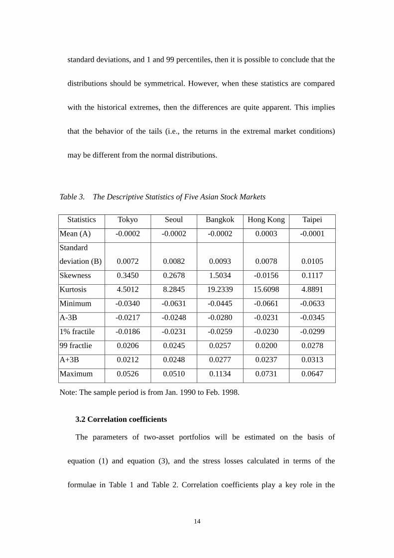
To understand the data structure primarily, the descriptive statistics of daily

returns are summarized in Table 3. Table 3 shows that the means of daily return

series are all near zero, and the standard deviations of five market returns are not

apparently different and are all in the range of 0.72% and 1.05%. However, the

skewness and kurtosis are very different among the five markets. The skewness of

Hong Kong is negative, but for the other four markets it is slightly positive.

Furthermore, the kurtosis of the five markets is higher than 3.0, the value held by a

normal distribution. The information given in Table 3 indicates that most of

empirical distributions are centralized at zero, but may have quite different types of

peaks and tails in the respective markets.

Table 3 also presents the sample means plus (minus) three times the standard

deviations, 1 and 99 percentiles, and historical maxima and minima. If the data

structure is judged from the relative positions of means plus (minus) three times

14

standard deviations, and 1 and 99 percentiles, then it is possible to conclude that the

distributions should be symmetrical. However, when these statistics are compared

with the historical extremes, then the differences are quite apparent. This implies

that the behavior of the tails (i.e., the returns in the extremal market conditions)

may be different from the normal distributions.

Table 3. The Descriptive Statistics of Five Asian Stock Markets

Statistics Tokyo Seoul Bangkok Hong Kong Taipei

Mean (A) -0.0002 -0.0002 -0.0002 0.0003 -0.0001

Standard

deviation (B)

0.0072

0.0082

0.0093

0.0078

0.0105

Skewness 0.3450 0.2678 1.5034 -0.0156 0.1117

Kurtosis 4.5012 8.2845 19.2339 15.6098 4.8891

Minimum -0.0340 -0.0631 -0.0445 -0.0661 -0.0633

A-3B -0.0217 -0.0248 -0.0280 -0.0231 -0.0345

1% fractile -0.0186 -0.0231 -0.0259 -0.0230 -0.0299

99 fractlie 0.0206 0.0245 0.0257 0.0200 0.0278

A+3B 0.0212 0.0248 0.0277 0.0237 0.0313

Maximum 0.0526 0.0510 0.1134 0.0731 0.0647

Note: The sample period is from Jan. 1990 to Feb. 1998.

3.2 Correlation coefficients

The parameters of two-asset portfolios will be estimated on the basis of

equation (1) and equation (3), and the stress losses calculated in terms of the

formulae in Table 1 and Table 2. Correlation coefficients play a key role in the

15

calculation of stress losses. The historical correlation coefficients will be used in

Kupiec’s (1998) model. They will also be employed by weighting the conditional

probabilities of core asset being in ‘hectic’ periods in Kim and Finger’s (1999)

model.

The historical correlation matrix calculated by means of the full sample data is

shown in Table 4. It is immediately evident that the correlation coefficients between

any two markets are not very high. The specific cases of Hong King and Seoul, and

Hong Kong and Bangkok are used to illustrate the estimations of aggregated stress

losses of two-asset portfolios since these markets were influenced most deeply by

the Asian financial crisis in 1997. Furthermore, we shall assume that the Hong

Kong market position is the core asset (and thus carries a higher investment weight),

and the other two markets positions (Seoul and Bangkok) are the non-core assets

(and thus attract lower investment weights).

Table 4. The Linear Correlation Coefficients of Returns among Five Asian Stock Markets Tokyo Seoul Bangkok Hong Kong Taipei

Tokyo 1

Seoul 0.1084 1

Bangkok 0.1650 0.2252 1

Hong Kong 0.3052 0.1713 0.3737 1

Taipei 0.1870 0.1194 0.1785 0.1931 1

3.3 Backtesting

16

In order to check the accuracy of the models considered in this paper, we

performed backtests using the method developed by Kupiec (1995). Let P be

the ‘theoretical failure rate’, which is defined as the proportion of the total of

estimated stress losses being exceeded in a given sample. And let TN / be the

‘observed failure rate’, which is defined as the number of observations ( N ) in

which estimated stress loss is exceeded, over the total observed data (T ). Kupiec

(1995) developed a likelihood ratio test with the test statistic being:

])/())/(1log[(2])1log[(2 NNTNNT TNTNppLR −− −+−−= , (4)

which is a distributed chi-square with one degree of freedom. If LR is

significant, then the accuracy of our model is rejected. Conversely, one can also

define the non-rejection regions of N such that the accuracy of our model will not

be rejected. Since the sample size of our return data is 1708 (T=1708), the

non-rejected regions of alternative ‘theoretical failure rates’ at significance levels,

can be set at 0.01, 0.05 and 0.10 respectively. These non-rejected regions are

summarized in Table 5. For instance, if N =0.005 and significance level=0.05, the

non-rejection region is 3< N <15.

17

Table 5. Non-rejection regions for number of failures (N) (Sample = 1708) Critical probabilities Significant level=0.01 Significant level =0.05 Significant level =0.10

0.0100 0.9900 7<N<29 9<N<26 10<N<25

0.0075 0.9925 4<N<24 6<N<21 7<N<20

0.0050 0.9950 2<N<18 3<N<15 4<N<14

0.0025 0.9975 N<11 N<9 1<N<9

0.0020 0.9980 N<10 N<8 N<7

0.0015 0.9985 N<8 N<7 N<6

0.0010 0.9990 N<7 N<5 N<5

0.0005 0.9995 N<5 N<4 N<3

3.4 Empirical results

The estimated results of Kupiec’s (1998) and Kim and Finger’s (1999) models

are presented in Table 6 and Table 7 respectively. The estimates in Table 6 show

that the stress losses fall in the range of 0.93% and 2.15%. The absolute numbers of

the data sample exceeding estimated stress losses (shown in the corresponding

parentheses) indicate that the predictive accuracy of Kupiec’s (1998) model can be

rejected, if we use the information provided in the Table 5.

Table 6. Stress Losses Estimations of Two-asset Portfolios with Different Investment Weights in Bivariate Kupiec’s model ( 002.0=α )

Hong Kong Weights

(HK: Others) 60:40 75:25 90:10 Stock markets

Investment strategies

Long Short Long Short Long Short

Long 0.0149 (25)

0.0120 (28)

0.0176 (22)

0.0161 (15)

0.0204 (17)

0.0201 (18)

Seoul

Short 0.0117 (36)

0.0153 (27)

0.0156 (22)

0.0181 (19)

0.0195 (19)

0.0209 (13)

18

Long 0.0173 (27)

0.0097 (38)

0.0191 (22)

0.0146 (14)

0.0210 (19)

0.0195 (21)

Bangkok

Short 0.0093 (44)

0.0177 (25)

0.0141 (21)

0.0196 (20)

0.0190 (18)

0.0215 (12)

Note: the number of sample exceeding estimated stress losses are in the corresponding parentheses.

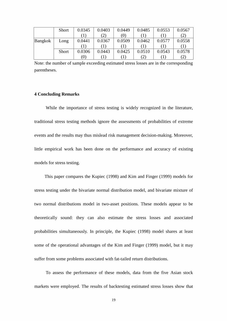
The results in Table 7 demonstrate that the stress losses are in the range of 3.06%

and 5.78%. The numbers of sample exceeding estimated stress losses (shown in the

corresponding parentheses) suggest that the predictive accuracy of Kim and

Finger’s (1999) model should not be rejected, and that all of these numbers are all

less than 2. Accordingly, we can conclude that the Kim and Finger (1999) model is

much more precise than the Kupiec’s (1998) model. A common characteristic of

both models is that the estimated stress losses are symmetrical when the investment

strategy is either one-way (i.e., long or short positions in both markets) or mixed

(i.e., a long position in one market and a short position in the other market).

However, the estimated stress losses from former model are insufficient to cover

the extremal losses. Put differently, the estimated stress losses from the Kim and

Finger (1999) model can satisfy the requirements of backtests.

Table 7. Stress Losses Estimations of Two-asset Portfolios with Different Investment Weights in Bivariate Kim and Finger’s model ( 002.0=α )

Hong Kong Weights

(HK: Others) 60:40 75:25 90:10 Stock markets

Investment strategies

Long Short Long Short Long Short

Seoul Long 0.0402 (1)

0.0344 (1)

0.0485 (1)

0.0449 (1)

0.0567 (1)

0.0553 (1)

19

Short 0.0345 (1)

0.0403 (2)

0.0449 (0)

0.0485 (1)

0.0553 (1)

0.0567 (2)

Long 0.0441 (1)

0.0367 (1)

0.0509 (1)

0.0462 (1)

0.0577 (1)

0.0558 (1)

Bangkok

Short 0.0306 (0)

0.0443 (1)

0.0425 (1)

0.0510 (2)

0.0543 (1)

0.0578 (2)

Note: the number of sample exceeding estimated stress losses are in the corresponding parentheses.

4 Concluding Remarks

While the importance of stress testing is widely recognized in the literature,

traditional stress testing methods ignore the assessments of probabilities of extreme

events and the results may thus mislead risk management decision-making. Moreover,

little empirical work has been done on the performance and accuracy of existing

models for stress testing.

This paper compares the Kupiec (1998) and Kim and Finger (1999) models for

stress testing under the bivariate normal distribution model, and bivariate mixture of

two normal distributions model in two-asset positions. These models appear to be

theoretically sound: they can also estimate the stress losses and associated

probabilities simultaneously. In principle, the Kupiec (1998) model shares at least

some of the operational advantages of the Kim and Finger (1999) model, but it may

suffer from some problems associated with fat-tailed return distributions.

To assess the performance of these models, data from the five Asian stock

markets were employed. The results of backtesting estimated stress losses show that

20

the Kim and Finger (1999) model is preferred for performing stress tests. Our results

imply that Kim and Finger (1999) model possess superior precision in capturing the

fat-tailed nature of emergent market return distributions, and in determining the

extremal correlation between assets in stressful market conditions. These empirical

results may be useful to risk managers who are interested in Asian stock markets.

21

References

Bank for International Settlement, 1995, An Internal Model-Based Approach to

Market Risk Capital Requirements, Basle Committee on Banking Supervision, Basle,

Switzerland.

Bank for International Settlement, 1996, Amendment to the Capital Accord to

Incorporate Market Risks, Basle Committee on Banking Supervision, Basle,

Switzerland.

Bank for International Settlement, 1999, Performance of Models-Based Capital

Charges for Market Risk, Basle Committee on Banking Supervision, Basle,

Switzerland.

Berkowitz, J., 1999, A Coherent Framework for Stress Testing, Working Paper, FEDS

1999-29, Federal Reserve Board.

Best, P., 1998, Implementing Value at Risk, John Wiely & Sons Ltd.

Best, P., 1999, VaR versus Stress Testing, Derivatives Week (Nov. 8th), 6-7.

Blanco, C., 1999, Complementing VaR with Stress Tests, Derivatives Week (Aug.

9th), 5-6.

Breuer, T and Krenn, G., 1999, Guidelines on Market Risk Volume 5 --- Stress

Testing, Austrian National Bank.

Derivatives Policy Group, 1995, Framework for Voluntary Oversight, US.

Dunbar, N. and R. Irving, 1998, This Is the Way the World Ends, Risk (Dec), 28-32.

22

International Organization of Securities Commissions, 1995, The Implications for

Securities Regulators of the Increased Use of Value at Risk Models by Securities

Firms, Technical Committee, Montreal, Canada.

International Organization of Securities Commissions, 1999, Recognizing A Firm’s

Internal Market Risk Model for the Purposes of Calculating Required Regulatory

Capital: Guidance to Supervisors, Technical Committee, Montreal, Canada.

Kim, J. and C. Finger, 1999, A Stress Test to Incorporate Correlation Breakdown,

working paper, RiskMetrics Group.

Kimball, R., 2000, Failure in Risk Management, New England Economic Review,

Jan./Feb, 3-12.

Kupiec, P., 1995, Techniques for Verifying the Accuracy of Risk Measurement

Models, Journal of Portfolio Management, summer, 73-84.

Kupiec, P., 1998, Stress Testing in a Value at Risk Framework, Journal of Derivatives,

Fall, 7-24.

RiskMetrics Group, 1999, Risk Management --- A Practical Guide.

Wang, S., S. Wu and H. Chung, A New Approach of Stress Testing for Stock

Portfolios and its Application to the Taiwan Stock Market, Asian Pacific Journal of

Economics and Business, 4, 52-73.

Zangari, P., 1997, Catering for an Event, Risk, 10, 34-36.

23

Appendix 1

Since

ΣΣ

ΣΣ

22

12

21

11

2

1

||,~

~~~

t

tNt NR

µµ

, the return of the portfolio can be calculated as

tttt RWRWV 1122~~~ +=∆ .

If the stress scenario of core assets is defined as ],...,,[~2122 kt rrrRR == , then

tttt RWRWV 1122~~ +=∆ .

The distribution of tR1~ conditioned on the ],...,,[~

2122 kt rrrRR == can be derived

as ),(~|~22

~1 ccRRt NRt

Σ= µ ,

where )( 221

22121 µµµ −ΣΣ+= − Rc , and 211

221211 ΣΣΣ−Σ=Σ −c .

Therefore, the return to this portfolio can be written as

2222~1122~ |~|~

RRtttRRt ttRWRWV == +=∆ , and their expected value and variance

are ))(()~|~( 221

2212112212222 µµµ −ΣΣ++=+==∆ − RWRWWRWRRVE ttcttt , and

==∆ )~|~( 22 RRVV tTtt WW 121

12212111 )( ΣΣΣ−Σ − respectively.

The estimated stress loss of the portfolio can be computed like the VaR:

StressVaR(95%)= )~|~()~|~( 2295.022 RRVVZRRVE tt =∆−=∆ =

)( 21

2212122 RWRW tt−ΣΣ+ -1.65 T

tt WW 1211

2212111 )( ΣΣΣ−Σ − .

So the expected value of stress loss is

E[StressVaR(95%)]= )~|~( 22 RRVE t =∆ = ))(( 221

22121122 µµ −ΣΣ++ − RWRW tt .

24

Appendix 2

Since the marginal distribution x can shown as

)(1),(~

)(),(~

22

11

periodhecticwprobwithN

periodquietwprobwithNx

xx

xx

−=

=

σµ

σµ,

the conditional probabilities of x being from ‘hectic’ periods can be calculated

by tα using the Bayesian theorem:

tα =),|()(),|()1(

),|()1(

1122

22

xxtxxt

xxt

xfwxfwxfw

σµσµσµ

+−−

.

The tα can be used as weight factors for estimating the parameters in Kim and

Finger’s (1999) model (equation 3). Thus,

∑=

=n

tttx x

12 αµ , ∑

=

=n

ttty y

12 αµ , ∑

=

−=n

txttx x

1

22

22 )( µασ ,

∑=

−=n

txttx x

1

22

22 )( µασ , and

∑

∑

=

=

−−= n

ttyx

n

tytxtt

yx

yx

122

122

22

))((

ασσ

µµαρ .

0

50

100

150

200

250

01/04/90

05/04/90

09/04/90

01/04/91

05/04/91

09/04/91

01/04/92

05/04/92

09/04/92

01/04/93

05/04/93

09/04/93

01/04/94

05/04/94

09/04/94

01/04/95

05/04/95

09/04/95

01/04/96

05/04/96

09/04/96

01/04/97

05/04/97

09/04/97

01/04/98

Figure 1. The Standardized Indices of Five Asian Stock M arkets

HK index

BK index

SL indexTW index

TK index