COORDINATED PATH FOLLOWING

OF

MULTIPLE AUTONOMOUS VEHICLES

By

Reza Ghabcheloo

SUBMITTED IN PARTIAL FULFILLMENT OF THE

REQUIREMENTS FOR THE DEGREE OF

DOCTOR OF PHILOSOPHY

AT

INSTITUTO SUPERIOR TECNICO

TECHNICAL UNIVERSITY OF LISBON

MAY 29, 2007

c© Copyright by Reza Ghabcheloo, 2007

“If you can’t explain it simply, you

don’t understand it well enough.”

Albert Einstein

i

ii

ABSTRACT

The thesis addresses the problem of steering a group of autonomous vehicles along given

spatial paths while holding a desired inter-vehicle formation pattern. In short, the problem

of Coordinated Path-Following (CPF). The solution proposed unfolds in two basic steps.

First, a path-following control law is derived that drives each vehicle to its assigned path

no matter what the speed profile of the vehicle is. In the methodology adopted for path-

following, to each vehicle there corresponds a virtual reference target that moves along the

path. A conveniently defined error vector that captures the “generalized” distance between

the vehicle and the target is then driven asymptotically to zero. In the second step, the

speeds of all vehicles are adjusted so as to synchronize the positions of the correspond-

ing virtual targets (also called coordination states), thus achieving coordination along the

paths. In the problem formulation, it is explicitly assumed that each vehicle transmits its

coordination state to a subset of the other vehicles only, as determined by the communica-

tions topology adopted. This allows for explicit consideration of stringent communication

constraints.

The thesis is organized as follows. Chapter 1 is the Introduction: it contains motivating

examples and a summary of the contributions of the thesis. Chapter 2 offers a local solution

to the CPF problem using a simple algorithm that builds on linearization techniques and

gain scheduling control theory. In Chapter 3, Lyapunov-based techniques and graph theory

are brought together to yield a global nonlinear decentralized control structure for CPF.

Both bi-directional and uni-directional communication topologies are studied. Chapter 4

addresses important stability and performance issues that arise from the consideration of

complex underactuated vehicle dynamics as well as inter-vehicle communication losses

and time delays. Finally, Chapter 5 contains the conclusions and discusses challenging

issues that warrant further research.

Key words: Coordinated path-following, Coordination control, Path-following, Commu-

nication constraints, Switching communication topologies, Time delays, Wheeled robots,

Underactuated vehicles, Marine vehicles.

iii

iv

RESUMO

Esta tese aborda o problema do seguimento coordenado de caminhos de multiplos veıculos

autonomos. Na sua essencia, o problema consiste em coordenar um conjunto de veıculos

de modo a que sigam caminhos estabelecidos, ao mesmo tempo que mantem um padrao

geometrico desejado. A solucao proposta desenrola-se em dois passos. Primeiro, con-

stroi-se uma lei de controlo que obriga cada veıculo a convergir para o caminho que lhe

esta atribuıdo, qualquer que seja o seu perfil de velocidade. A estrategia adoptada requer

a construcao de um veıculo-referencia virtual que se movimenta ao longo do caminho.

Define-se um vector de erro que capta a distancia “generalizada” entre o veıculo real e

o virtual, e conduz-se esse erro assimptoticamente para zero. No segundo passo, as ve-

locidades sao ajustadas de modo a sincronizar as posicoes espaciais (tambem denominadas

estados da coordenacao) dos veıculos virtuais e atingir o padrao gometrico desejado. Na

formulacao do problema, assume-se explicitamente que existem restricoes fortes aos tipos

de comunicacoes que se podem estabelecer entre os veıculos. Em particular, assume-se que

cada veıculo so pode comunicar com um subconjunto de veıculos na sua vizinhanca.

A tese esta organizada em cinco capıtulos. O Capıtlo 1 introduz o problema a estu-

dar atraves de exemplos e apresenta as contribuicoes principais da tese. No Capıtulo 2

apresenta-se uma solucao - denominada local - para o problema do seguimento coordenado

de caminhos recorrendo a tecnicas de linearizacao e comutacao de ganhos. No Capıtulo 3

levantam-se as restricoes mencionadas e consideram-se formacoes arbitrarias de veıculos.

Recorrendo a tecnicas de Lyapunov e teoria dos Grafos, derivam-se leis descentralizadas e

globais para o controlo coordenado de multiplos veıculos. O Capitulo 4 analisa o impacte

de falhas temporarias e atrasos nas comunicacoes na estabilidade e desempenho de uma

formacao de veıculos. Finalmente, o Capitulo 5 contem as conclusoes e discute problemas

para investigacao futura.

Palavras-Chave: Seguimento coordenado de caminhos, Controlo cooperativo, Seguimento

de caminhos, Redes de Comunicacoes e Controlo, Sistemas com atrasos, Sistemas com fal-

has, Veıculos sub-actuados, Veıculos Terrestres, Veıculos Marinhos.

v

vi

ACKNOWLEDGEMENTS

I would like to start by saying that the last few years have been the most “colorful and

spicy” of my life because I truly had the opportunity to meet and get to know people from

different countries, with different customs and a wide range of cultural backgrounds. In the

process, I learned how boring life would be without these differences and contrasts. I am

pleased that I became part of a community where I could appreciate how each individual

brings to a common environments his or her unique intrinsic beauty, strength, and values.

I am also deeply grateful to all the teachers that opened my eyes and guided my steps in

the long and winding (and yet truly challenging and exciting) road to the fantastic world of

research.

First and foremost, I thank my thesis advisor, Professor Antonio Pascoal, who was not

only scientifically but also socially my teacher and guide. I am grateful to his continuous

stream of ideas and insightful comments, excellent guidance and patience, and availability

to listen to my concerns and hardships, thus absorbing some of the pressure that I experi-

enced at times. Undoubtedly, he was the most influential person during my PhD studies

and I can only wish that the link that we established will continue in the years to come.

He is truly a good friend. My special thanks go to my thesis co-advisor, Professor Carlos

Silvestre, for his encouraging and useful comments and for always being helpful and giving

good insight into the problems. I thank both of them for giving me support and offering me

countless opportunities.

Professor Pedro Aguiar came to ISR in the middle of my PhD research. However, he

was extremely influential in shaping its final stage. I was lucky to have him as my next door

neighbor, always available for discussions and solid advice on theoretical issues. He truly

helped me open new horizons and develop new concepts that materialized in the form of

joint publications. I am indebted to his guidance and thought provoking discussions. I am

also indebted to Professor Isaac Kaminer for his helpful comments, exciting discussions

and tremendous insight on the practical implications of the theoretical results derived. I

thank him for giving me the opportunity to visit the NPS and hosting me in Monterey,

California as a good friend. I am also obliged to Professor Kristing Petterson for being kind

enough to invite me to spend three months at the NTNU and for creating a pleasant and

challenging research atmosphere that I truly appreciated. My special gratitude goes also to

Professor Michael Athans for his cheerful disposition and encouragement and for giving

vii

me great insight into control and estimation theory. I would also like to thank Professor

Joao Hespanha for his insight advice and helpful comments on some of the work that we

did jointly.

To Professor Isabel Ribeiro, the Director of ISR, go my special thanks for her determi-

nation in pursuing the policy of attracting and encouraging foreign PhD students to come

and stay in Portugal and for making the atmosphere of ISR a friendly and motivating one.

I would like to thank all the institutions that supported this work, and in special the FCT

(Fundacao para a Ciencia e a Tecnologia) for providing me with a PhD grant1.

I also thank Professor Joao Lemos and Professor Jose Sa da Costa for having kindly

agreed to participate in my thesis research and final PhD committees, and for giving me

solid advice on how to shape the thesis. My appreciation goes also to Professor Jorge

Martins de Carvalho for his participation in my PhD committee.

I wish to thank my father, mother, brother and sister, although far, for giving me courage

and strength through their understanding and moral support. My deepest thanks go to

Niina for giving me continuous hope and courage, specially through final stages of my

PhD research. I also express my gratitude to the Pestana’s family, Eduarda and Rui, who

played the role of my family and friends in Portugal. In this regard, I can never forget my

Brazilian friends Rodrigo, Ana, and Danilo.

Finally, I wish to thank Rita, Sandra, Karim, Alex, Francisco, Nuno, Guilherme, Luis,

Rufino, and Sajjad for their friendship and a pleasant working atmosphere.

Lisbon, Portugal Reza Ghabcheloo

December 28, 2006

1This work was supported by the Portuguese FCT POSI program under framework QCA III. It was also

partly supported by MAYA-Sub of the AdI, project GREX / CEC-IST (Contract No. 035223), and the FCT-

ISR/IST plurianual funding program (through the POS-Conhecimento Program initiative in cooperation with

FEDER).

viii

TABLE OF CONTENTS

Abstract iii

Resumo v

Acknowledgements vii

List of Figures xii

1 Introduction 1

1.1 Coordinated path-following . . . . . . . . . . . . . . . . . . . . . . . . . . 5

1.1.1 Path-following . . . . . . . . . . . . . . . . . . . . . . . . . . . . 5

1.1.2 Coordination . . . . . . . . . . . . . . . . . . . . . . . . . . . . . 7

1.2 Coordinated path-following: a simple example . . . . . . . . . . . . . . . . 11

1.3 Literature review . . . . . . . . . . . . . . . . . . . . . . . . . . . . . . . 16

1.3.1 Coordinated path-following . . . . . . . . . . . . . . . . . . . . . 17

1.3.2 Communication topologies and graph theory . . . . . . . . . . . . 19

1.4 Publications and thesis contributions . . . . . . . . . . . . . . . . . . . . . 24

1.5 Structure of the thesis . . . . . . . . . . . . . . . . . . . . . . . . . . . . . 28

2 Linearization techniques: Wheeled robots 31

2.1 Path-following: single vehicle . . . . . . . . . . . . . . . . . . . . . . . . 32

2.1.1 Decoupling algorithm . . . . . . . . . . . . . . . . . . . . . . . . 36

2.1.2 State transformation . . . . . . . . . . . . . . . . . . . . . . . . . 40

2.2 Vehicle coordination control . . . . . . . . . . . . . . . . . . . . . . . . . 43

2.2.1 Leader-follower . . . . . . . . . . . . . . . . . . . . . . . . . . . . 46

2.2.2 Gateway . . . . . . . . . . . . . . . . . . . . . . . . . . . . . . . 48

2.3 Stability of the coordinated path-following control system . . . . . . . . . . 50

2.3.1 Decoupling algorithm . . . . . . . . . . . . . . . . . . . . . . . . 50

2.3.2 State transformation . . . . . . . . . . . . . . . . . . . . . . . . . 52

2.4 Robustness against vehicle failures . . . . . . . . . . . . . . . . . . . . . . 53

2.5 Simulations . . . . . . . . . . . . . . . . . . . . . . . . . . . . . . . . . . 57

2.5.1 Control of direction of motion . . . . . . . . . . . . . . . . . . . . 57

2.5.2 Coordinated path-following . . . . . . . . . . . . . . . . . . . . . 58

ix

2.5.3 Coordinated path-following with vehicle failures . . . . . . . . . . 59

2.6 Summary . . . . . . . . . . . . . . . . . . . . . . . . . . . . . . . . . . . 61

3 Fixed communication topologies: Wheeled robots,

fully actuated marine vehicles 65

3.1 Mathematical preliminaries . . . . . . . . . . . . . . . . . . . . . . . . . . 65

3.1.1 Stability definitions and related theorems . . . . . . . . . . . . . . 66

3.1.2 Graph theory . . . . . . . . . . . . . . . . . . . . . . . . . . . . . 72

3.2 Path-following: single vehicle . . . . . . . . . . . . . . . . . . . . . . . . 82

3.2.1 Wheeled robots . . . . . . . . . . . . . . . . . . . . . . . . . . . . 82

3.2.2 Fully actuated marine vehicles . . . . . . . . . . . . . . . . . . . . 91

3.3 Vehicle coordination control. Fixed communication topologies . . . . . . . 95

3.3.1 Coordination error dynamics . . . . . . . . . . . . . . . . . . . . 95

3.3.2 Bi-directional communications . . . . . . . . . . . . . . . . . . . . 98

3.3.3 Time-varying pattern tracking . . . . . . . . . . . . . . . . . . . . 106

3.3.4 Uni-directional communications . . . . . . . . . . . . . . . . . . . 108

3.3.5 Truly decentralized vehicle coordination . . . . . . . . . . . . . . . 112

3.3.6 Path-following and coordination control interconnection . . . . . . 117

3.4 Simulations . . . . . . . . . . . . . . . . . . . . . . . . . . . . . . . . . . 124

3.4.1 Bi-directional communications . . . . . . . . . . . . . . . . . . . . 124

3.4.2 Uni-directional communications . . . . . . . . . . . . . . . . . . . 125

3.5 Summary . . . . . . . . . . . . . . . . . . . . . . . . . . . . . . . . . . . 125

4 Switching communication topologies: General autonomous vehicles 131

4.1 Problem statement . . . . . . . . . . . . . . . . . . . . . . . . . . . . . . 131

4.1.1 Path-following control . . . . . . . . . . . . . . . . . . . . . . . . 133

4.1.2 Vehicle coordination . . . . . . . . . . . . . . . . . . . . . . . . . 134

4.2 Preliminaries and basic results . . . . . . . . . . . . . . . . . . . . . . . . 135

4.2.1 Graph theory . . . . . . . . . . . . . . . . . . . . . . . . . . . . . 135

4.2.2 Brief connectivity losses . . . . . . . . . . . . . . . . . . . . . . . 136

4.2.3 Connected in mean topology . . . . . . . . . . . . . . . . . . . . . 139

4.2.4 System interconnections. Systems with brief instabilities . . . . . . 141

4.3 Coordinated path-following: no communication delays . . . . . . . . . . . 144

4.3.1 Brief connectivity losses . . . . . . . . . . . . . . . . . . . . . . . 145

4.3.2 Uniform switching topology . . . . . . . . . . . . . . . . . . . . . 148

4.4 Coordinated path-following: delayed information . . . . . . . . . . . . . . 151

4.5 Underactuated autonomous vehicles . . . . . . . . . . . . . . . . . . . . . 155

4.5.1 Path-following . . . . . . . . . . . . . . . . . . . . . . . . . . . . 155

4.5.2 Coordinated path-following . . . . . . . . . . . . . . . . . . . . . 160

4.6 An illustrative example . . . . . . . . . . . . . . . . . . . . . . . . . . . . 166

4.7 Summary . . . . . . . . . . . . . . . . . . . . . . . . . . . . . . . . . . . 167

x

5 Concluding chapter 171

6 Appendix 173

6.1 Path-following control implementation . . . . . . . . . . . . . . . . . . . 173

6.2 Proofs . . . . . . . . . . . . . . . . . . . . . . . . . . . . . . . . . . . . . 174

xi

xii

LIST OF FIGURES

1.1 ASIMOV concept . . . . . . . . . . . . . . . . . . . . . . . . . . . . . . . 4

1.2 Underway replenishment . . . . . . . . . . . . . . . . . . . . . . . . . . . 5

1.3 Path-following problem . . . . . . . . . . . . . . . . . . . . . . . . . . . . 6

1.4 Coordination: triangle formation . . . . . . . . . . . . . . . . . . . . . . . 7

1.5 Coordination: in-line formation . . . . . . . . . . . . . . . . . . . . . . . . 7

1.6 Along-path distances: straight lines . . . . . . . . . . . . . . . . . . . . . . 8

1.7 Along-path distances: circumferences . . . . . . . . . . . . . . . . . . . . 8

1.8 Coordination: a general scheme . . . . . . . . . . . . . . . . . . . . . . . 9

1.9 CPF. Simple example with fixed communication topology . . . . . . . . . . 13

1.10 CPF. Simple example with communication losses . . . . . . . . . . . . . . 14

2.1 Frames and error variables. a wheeled robot . . . . . . . . . . . . . . . . . 32

2.2 D−methodology - state feedback . . . . . . . . . . . . . . . . . . . . . . . 39

2.3 D−methodology - output feedback case . . . . . . . . . . . . . . . . . . . 39

2.4 Angular speeds and spatial paths of the robot for different trimming speeds 40

2.5 Controller implementation, state transformation . . . . . . . . . . . . . . . 42

2.6 Comparison between the decoupling and state transformation methods . . . 42

2.7 Information flow diagram: Leader-Follower, Gateway, Neighbors . . . . . . 46

2.8 Root locus of the coordinated path-following system . . . . . . . . . . . . 52

2.9 Frame selection: Lines . . . . . . . . . . . . . . . . . . . . . . . . . . . . 58

2.10 Frame selection: Circumferences . . . . . . . . . . . . . . . . . . . . . . . 58

2.11 The effect of choosing different Serret-Frenet frames for the same geomet-

rical path . . . . . . . . . . . . . . . . . . . . . . . . . . . . . . . . . . . 59

2.12 Coordinated path-following: Gateway configuration, trajectories . . . . . . 60

2.13 Coordinated path following: Gateway configuration, vehicle speeds . . . . 60

2.14 Coordinated path-following: Gateway configuration, the coordination errors 61

xiii

2.15 Gateway configuration, failures . . . . . . . . . . . . . . . . . . . . . . . . 63

3.1 An undirected graph with an associated orientation . . . . . . . . . . . . . 75

3.2 Graph example, directed . . . . . . . . . . . . . . . . . . . . . . . . . . . 80

3.3 Frames and error variables. a wheeled robot . . . . . . . . . . . . . . . . . 83

3.4 Frames and error variables. a marine vehicle . . . . . . . . . . . . . . . . . 92

3.5 Augmented graph. vL known only to the virtual leader . . . . . . . . . . . 113

3.6 Interconnected system . . . . . . . . . . . . . . . . . . . . . . . . . . . . 119

3.7 In-line formation, constant C, bi-directional communications . . . . . . . . 127

3.8 Triangular formation, constant C, bi-directional communications . . . . . . 128

3.9 Coordination of 2 vehicles, varying C, bi-directional communications . . . 129

3.10 Coordination of 3 vehicles, uni-directional communications . . . . . . . . . 130

4.1 Interconnected system . . . . . . . . . . . . . . . . . . . . . . . . . . . . 147

4.2 Coordinated path-following of 3 AUVs with communication losses and

time delays. Trajectories of the vehicles . . . . . . . . . . . . . . . . . . . 168

4.3 Coordinated path-following of 3 AUVs with communication losses and

time delays. Error variables . . . . . . . . . . . . . . . . . . . . . . . . . . 169

xiv

CHAPTER 1

INTRODUCTION

This thesis addresses the problem of coordinated path-following (CPF) whereby multiple

vehicles are required to follow pre-specified spatial paths while keeping a desired inter-

vehicle formation pattern in time. This problem is strongly motivated by mission scenarios

that occur naturally in marine robotics (Pascoal et al. 2000). Namely, in the operation of

multiple autonomous vehicles for fast acoustic coverage of the seabed. In this important

case, two or more vehicles are required to fly above the seabed at the same or different

depths, along geometrically similar spatial paths, and map the seabed using copies of the

same suite of acoustic sensors. By requesting that the vehicles traverse identical paths so as

to make the acoustic beam coverage overlap along the seabed, large areas can be covered

in a short time. This imposes constraints on the inter-vehicle formation pattern. Similar

scenarios can of course be envisioned for land and air vehicles.

The problem of coordinated path-following has only recently come to the forum. How-

ever, some of the key concepts involved can be in part traced back to the ASIMOV project

of the CEC coordinated by IST, that aimed at the coordinated control of marine robots. See

for example the following statement in (Pascoal et al. 2000).

“Three major stumbling blocks have thus far prevented demonstrating the po-

tential applications of Autonomous Underwater Vehicle (AUVs) to demand-

ing industrial and scientific missions. Namely, i) the lack of reliable naviga-

tion systems, ii) the impossibility of transmitting data at high rates between

1

2

the AUV and a support ship at slant range, and iii) the unavailability of ad-

vanced mission control systems offer effectively affording end-users the tools

to seamlessly plan, program, and run scientific / industrial missions at sea,

while having access to ocean data in almost real-time so as to re-direct the

AUV mission, if required. As a contribution toward solving some of the above-

mentioned problems, the ASIMOV project puts forward the key concept of an

Autonomous Surface Vehicle (ASV) that will operate in close cooperation with

an AUV, as a mobile relay for fast communications. In the scenarios consid-

ered, the ASV will be equipped with a differential GPS receiver, an ultra short

baseline unit (USBL), a radio link, and a high data rate communication link

with the AUV that will be optimized for the vertical channel. By properly

maneuvering the ASV to always remain in the vicinity of a vertical line with

the AUV, a fast communication link can be established to transmit navigational

data from the DGPS and USBL units to the AUV and ocean data from the AUV

to the ASV, and subsequently to an end-user located on board a support ship or

on shore via an aerial link.”

The above concept is illustrated in Figure 1.1. Other scenarios can be envisioned, of which

the following are representative examples. See (Fossen 2002) and (Pascoal et al. 2006) and

the references therein.

• Image acquisition- Combined autonomous underwater vehicle control. This scenario

occurs when an underwater vehicle carries a strong light source and illuminates the

scenery around a second underwater vehicle that must follow a pre-determined path

and acquire images for scientific purposes.

• Fast acoustic coverage of the seabed - Combined autonomous underwater vehicle

control. In this important case, two vehicles are required to maneuver above the

seabed at identical or different depths, along parallel paths, and map the sea bottom

using two copies of the same suite of acoustic sensors (e.g. sidescan, mechanically

scanned pencil beam, and sub-bottom profiler). By requesting the vehicles to traverse

identical paths so as to make the acoustic beam coverage overlap on the seabed, large

3

areas can be covered quickly. One can also envision a scenario where the vehicles

use a set of vision sensors to inspect the same scenery from two different viewpoints

to try and acquire three-dimensional images of the seabed.

• Underway replenishment, or replenishment at sea- a challenging mission scenario.

“An underway replenishment operation is an operation where fuel, food, parts or

personnel are transferred from one vessel to another while both vessels are moving,

and is common in marine operations.” (Kyrkjebo 2007). In this situation, there is a

need to coordinate the two vessels, the mother vessel playing the role of leader and

the ship to be replenished that of follower, the vessels moving in a alongside kind of

formation. See Figure 1.2.

The above circle of ideas has spurred great interest and has led to the definition of some

challenging problems that are of the root of the key questions addressed in this thesis. From

a theoretical viewpoint, the plethora of problems that must be solved to achieve coordina-

tion of multiple vehicles spans a vast number of fields that include navigation, guidance,

and control. Here, we focus on the problem of coordinated motion control. At first inspec-

tion, this problem seems to fall within the domain of decentralized control. However, as

clearly pointed out by (Fax & Murray 2002a,b), it possesses several unique aspects that

pose new challenges to system designers. Among these, the following are worth stressing:

i) except for some cases in the area of aircraft control, the motion of one vehicle does

not directly affect the motion of the other vehicles, that is, the vehicles are dynamically

decoupled; the only coupling arises naturally out of the specification of the tasks that they

are required to accomplish together.

ii) there are strong practical limitations to the flow of information among vehicles,

which is severely restricted by the nature of the supporting communications network. In

marine robotics, for example, underwater communications (that rely on the propagation of

acoustic waves) are plagued with intermittent failures, delays, and multi-path effects. These

effects set tight limits on the effective communication bandwidths that can be achieved and

introduce latency in the measurements that are exchanged among the vehicles. As a rule,

no vehicle will be able to communicate with the entire formation and the vehicles cannot

4

Figure 1.1: ASIMOV project. AUV / ASC coordination

all communicate at the same time. It is therefore imperative to develop coordinated mo-

tion control strategies that can yield robust performance in the presence of communication

failures and switching communication topologies. New paradigms are required to address

these challenges, thus departing from classical centralized control methodologies.

Classical centralized controllers deal with systems in which a single controller pos-

sesses all the information needed to achieve desired control objectives, including stability

and performance requirements. However, in many applications like the one described be-

fore, it is impractical to exchange all the relevant information and convert the problem into

a centralized one. Thus the need to study and develop decentralized algorithms where sin-

gle local controllers act based on partial information to accomplish a common goal. For

example, to bring subsets of the states of networked systems to converge to a common value

(agreement problem). Over the past few years, there has been a flurry of activity in the area

of multi-agent networks with application to engineering and science problems. The thesis

exploits some of the ideas proposed in the literature and advances new ones. The main

theme of the work revolves around coordinated path-following, as explained below.

5

Figure 1.2: Underway replenishment. Source: US defence visual information center/public

release. ID: DN-SC-05-06680.

1.1 Coordinated path-following

Coordinated Path-Following (CPF) addresses the problem of steering a group of autonomous

vehicles along given spatial paths, while holding a desired inter-vehicle formation pattern.

The CPF control methodology is a “Divide to Conquer” approach. Using this framework,

path-following (in space) and inter-vehicle coordination (in time) can be essentially be

viewed as decoupled. Path-following for each vehicle amounts to reducing a conveniently

defined error variable to zero. Vehicle coordination is typically achieved by adjusting the

“speed” of each of the vehicles along its path according to information on the positions of a

set of neighboring vehicles, as determined by the topology of the communication network

adopted. No other kinematic or dynamic information is exchanged among the vehicles.

1.1.1 Path-following

Consider the autonomous underwater vehicle depicted in Figure 1.3, together a spatial path

Γ in the horizontal plane to be followed. It is assumed that the vehicle is equipped with

actuators capable of imparting the necessary forces and torques to it. In a great number

of cases, the vehicle may be underactuated. The problem of path-following can be briefly

stated as follows:

6

Ty

G

vt

y

b

B

t

n

path

yU

xU

T

U

s

ye

P

yF

xB

xF

Q

O

Figure 1.3: Path-following problem

Given a spatial path Γ, develop a feedback law for the control forces and torques acting

on the vehicle so that its centre of mass will converge asymptotically to the path while its

total speed tracks a desired temporal profile vd(t), t ≥ 0.

Consider again Figure 1.3, where P is an arbitrary point on the path and p denotes

its position in the inertial frame U. Let B≡xB,yB and F≡xF ,yF denote the

body-fixed frame and flow frame, respectively, of the vehicle both with origin at Q, its

centre of mass. Recall that the flow frame has its x−axis aligned with vehicle’s velocity

vector. Associated with P, consider the tangent frame T≡t,n, where t and n denote

the tangent and normal, respectively, to the path. The signed curvilinear abscissa of P

along the path is denoted s and is measured from some appropriate origin. With these

definitions, the problem of path-following is equivalently defined as that of driving the flow

frame F to the state-driven (time-varying) tangent frame T=T(s) while ensuring that

‖p(t)‖ tracks a desired speed profile. Under these conditions, Q tends to P, xF aligns itself

asymptotically with xT ≡ t, and s → vd . Several solutions to the problem of path-following

of a single vehicle will be presented in this thesis.

7

t

1 2 3

v

vv

G G G G

Figure 1.4: Coordination: triangle for-

mation

v

v

v

O

3

2

1

2G

3G

1G

Figure 1.5: Coordination: in-line forma-

tion

1.1.2 Coordination

In the most general set-up of the CPF problem, one is given a set of n ≥ 2 vehicles and

a set of n spatial paths Γk; k ∈ Nn := 1, ...,n and require that vehicle k follow path Γk.

We further require that the vehicles move along the paths in such a way as to maintain a

desired formation pattern compatible with the paths. The speeds at which they are required

to travel can be imposed in a number of ways; for example, by nominating one of the

vehicles as a formation leader, assigning a desired speed to it, and having the other vehicles

adjust their speeds accordingly. Figures 1.4 and 1.5 show the simple cases where 3 vehicles

are required to follow straight paths and circumferences Γi; i = 1,2,3, respectively, while

keeping a desired “triangle” or “in-line” formation pattern.

In the simplest case, the paths Γi may be obtained as simple parallel translations of a

“template” path Γt (Figure 1.4). A set of paths can also be obtained by considering the case

of scaled circumferences with a common centre and different radii Ri (Figure 1.5). In the

course of this thesis, more general paths and formation patterns will be considered.

Assuming that separate path-following controllers have been implemented for each ve-

hicle, it now remains to coordinate (that is, synchronize) the vehicle motions in time so

as to achieve a desired formation pattern. As will become clear throughout the thesis, this

will be achieved by adjusting the “speeds” of the vehicles as functions of the “along-path”

8

1

2

s1,2

s1

s2

1T

2T

Figure 1.6: Along-path distances:

straight lines

RR

12

l 1

l 2

s1

s2

2T

s1,2

1T

Figure 1.7: Along-path distances: cir-

cumferences

distances among them. To better grasp the key ideas involved in the computation of these

distances, consider for example the case of in-line formations maneuvering along parallel

translations of straight lines. For each vehicle i, let si denote the signed curvilinear abscissa

of the origin of the corresponding tangent frame Ti being tracked, introduced before.

Since the flow frame Fi tends asymptotically to Ti, it follows that the vehicles are

(asymptotically) coordinated or synchronized if

si, j(t) := si(t)− s j(t) → 0, t → ∞; i = 1, ..,n; i < j ≤ n. (1.1)

This shows that in the case of translated straight lines si, j is a good measure of the along-

path distances among the vehicles. Similarly, in the case of scaled circumferences an ap-

propriate measure of the distances among the vehicles is

si, j := si − s j; i = 1, ..,n; i < j ≤ n (1.2)

where si = si/Ri. See Figures 1.6 and 1.7.

Notice how the definition of si, j relies on a normalization of the lengths of the circumfer-

ences involved and is equivalent to computing the angle between vectors li and l j directed

from the centre of the circumferences to origin of the tangent frames Ti and T j, respec-

tively. In both cases, we say that the vehicles are coordinated if the corresponding along

path distance is zero, that is, si − s j = 0 or si − s j = 0. The extension of these concepts to a

9

2T

1T

Γ

Γ

2

1

ξ1,2

45º

Figure 1.8: A general coordination scheme

more general setting requires that each path Γi be parameterized in terms of a parameter ξi

that is not necessarily the arc length along the path. An adequate choice of the parameteri-

zation will allow for the conclusion that the vehicles are synchronized iff ξi = ξ j for all i, j.

For example, in the case of two vehicles following two circumferences with radii R1 and

R2 while keeping an in-line formation pattern, ξi = si/Ri; i = 1,2. This seemingly trivial

idea allows for the study of more elaborate formation patterns. As an example, consider

the problem depicted in Figure 1.8 where vehicles 1 and 2 must follow paths Γ1 and Γ2

while maintaining vehicle 2 ”to-the-left-and-behind” vehicle 1, that is, along a straight line

that makes an angle of 135 degrees with the positive direction of path Γ1. Let ξ1 = s1 and

ξ2 = s2

√2. It is clear that the vehicles are synchronized if they are on their assigned paths

and ξ1 −ξ2 = 0. Since the objective of the coordination is to synchronize the ξi’s, we will

refer to them as coordination states.

Consider the general problem of synchronizing n coordination states ξi; i ∈ Nn where

ξi corresponds to vehicle i and path Γi. For simplicity of exposition, assume the ve-

hicles are on their paths, thus avoiding at this introductory stage the problem of path-

following/coordination interaction. Let ui be the control signal of vehicle i available for co-

ordination. The objective is to derive a control law for ui; i∈Nn, so as to make ξ1 = ... = ξn

or, equivalently, (ξi−ξ j) = 0 for all i, j ∈Nn. It is further required that the fleet of vehicles

adopt a desired common speed profile vL , that is, ξi = vL ∀i ∈ Nn. This issue requires

clarification. Notice that the desired speed assignment is given in terms of the time deriva-

tives of the coordination states ξi, not in terms of the actual inertial speeds of the vehicles

10

undergoing synchronization. Assuming the vehicles have reached their paths, their speeds

degenerate into dsi

dt; i ∈ Nn and because

dξi

dt= dξi

dsi

dsi

dt= vL , it follows that dsi

dt= vL /dξi

dsi.

This yields dsi

dt= RivL for the example of the circumferences given above. With this speed

assignment, one does not have to specify the actual inertial speeds of the vehicles, but rather

those of their coordination states which are all equal to vL . In the most general setting vL

may be time-varying. For example, vL can be taken as an explicit function of time t or

of one of the coordination states ξi. At this point, two extremely important control design

constraints must be taken into consideration. The first type of constraint is imposed by the

topology of the inter-vehicle communications network, that is, by the types of links avail-

able for communications. The second type of constraint arises from the need to drastically

reduce the amount of information that is exchanged over the communications network. In

a typical case, it is assumed that the vehicles only exchange information on their “posi-

tions” along the paths (the coordination states). As a consequence the coordination laws

are necessarily of the form

ui = ui(ξi,ξ j : j ∈ Ni) (1.3)

where Ni ⊂Nn is the neighboring set, an index set that determines what coordination states

ξ j; j ∈ Ni are transmitted to vehicle i. With this control law, each vehicle i requires only

access to its own coordination state and to some or all of the coordination states of the

remaining vehicles, as defined by the index set Ni. Throughout the thesis, two types of

communication links are considered: i) bi-directional communication links, that is, if vehi-

cle i sends information to j, then j also sends information to i; formally, i ∈ N j ⇔ j ∈ Ni; ii)

uni-directional communication links, where i ∈ N j does not necessarily imply that j ∈ Ni.

Clearly, the index sets capture the type of communication structure that is available for ve-

hicle coordination. This suggests that the vehicles and the data links among them should be

viewed as a graph where the vehicles and the data links play the role of vertices of the graph

and edges connecting those vertices, respectively. It is thus natural that the machinery of

graph theory be brought to bear on the definition of the problem under study.

To better grasp the circle of ideas exposed, a very simple example of a CPF control

algorithm for two unicycle type robots is given next. The treatment is rather cursory and

most of the details are omitted. This subject will be fully studied in the main body of the

11

thesis which will address the problem of CPF for multiple underactuated vehicles, general

types of paths and formation patterns, and switching communication networks.

1.2 Coordinated path-following:

a simple example

Consider the problem of coordinated path-following control for two wheeled vehicles of

the unicycle type in the x− y plain. Each vehicle is required to follow a horizontal straight

line along the x−axis while keeping an in-line formation pattern along the y−axis, that is,

the vehicles are required to reach agreement on the x−coordinate. Let the equations of

motion of each vehicle be described by

x = vcosψ

y = vsinψ

where the forward speed v and the heading angle ψ are taken as the control signals. We will

refer to the vehicles as V1 and V2 and use subscripts 1 and 2 to distinguish between their

states. We further denote by Γi; i = 1,2 the paths to be followed by the vehicles, where

Γ1 and Γ2 are obtained by shifting the x−axis along the vertical coordinate y by ∆1s and

∆2s , respectively. Vehicle i; i = 1,2 can be driven to the desired path Γi using the heading

control

ψi = −sign(vi)sin−1[2

πtan−1 y−∆i

s

∆], (1.4)

where sign(.) is the sign function and ∆ > 0 is a tuning variable that is commonly referred

in the literature as the LOS1 distance. The resulting closed-loop dynamics in y are given by

yi = −2|vi|π

tan−1 yi −∆is

∆,

thus guaranteeing that yi → ∆is and ψi → 0 as t → ∞, if vi 9 0.

For each vehicle, its dynamics along the x−coordinate can be written as

xi = vi +di

1Line Of Sight

12

where di = vi(cosψi − 1) and di vanishes as t → ∞, since so does ψi. In what follows,

we assume that di = 0; i = 1,2 to simplify the presentation of the key ideas involved in

synchronization. Later throughout the thesis, we will consider the case when di 6= 0.

Consider a coordination problem in which the vehicles are required to agree on the

coordination state xi and follow a common speed profile vL (t). Assume that the vehicles

exchange information on their x−coordinate positions only. Coordination can be achieved

using the control law

x1 = v1 = −a1(x1 − x2)+ vL

x2 = v2 = −a2(x2 − x1)+ vL

(1.5)

for some ai > 0. To prove agreement between x1 and x2, let e = x1 − x2. This yields

e = −(a1 +a2)e and e converges exponentially to zero. Therefore, x1 and x2 tend to vL as

t → ∞. Implementing the control signal (1.5) requires that both vehicles know the speed

profile vL (t) in advance. While this is a plausible assumption, it can be alleviated when

vL is constant, as follows. Let V1 play the role of a leader that sets the formation speed

vL , and let V2 be required to learn it. Set a new coordination control law as

x1 = −a1(x1 − x2)+ vL

for V1 and

x2 = −a2(x2 − x1)+b2eI

eI = x1 − x2

for V2, where b2 > 0 and eI is an auxiliary “integral” state. Let e := x1−x2 and xc := (e,eI)T .

Then, xc = Axc +(vL ,0)T where

A =

(

−(a1 +a2) −b2

1 0

)

.

Clearly, A is Hurwitz. In the special case where b2 = a1a2, A has two eigenvalues at −a1

and −a2. Therefore xc → 0 exponentially if vL is constant. As a consequence, e → 0 as

t → ∞, and x1, x2 tend to vL . If vL has a bounded time derivative, xi−vL will be bounded.

Simulations were performed to visualize the time trajectories of the states in the above-

mentioned example. Figure 1.9 illustrates the simulations for the case where vL = 0.5[s−1],

13

0 5 10 15 20 25 300.45

0.46

0.47

0.48

0.49

0.5

0.51

0.52

0.53

0.54

0.55

time [s]

speed [m

/s]

vL

V1

V2

(a) Vehicle speeds

0 2 4 6 8 10 12 14

−4

−3

−2

−1

0

1

2

3

4

5

6

x [m]

y [m

]

V1

V2

(b) Vehicle trajectories

0 5 10 15 20 25 300

0.5

1

1.5

2

2.5

3

time [s]

[m]

V1

V2

(c) y1 −∆1s and y2 −∆2

s

0 5 10 15 20 25 300

0.05

0.1

0.15

0.2

0.25

0.3

0.35

time [s]

[m]

(d) x1 − x2

Figure 1.9: Simple example: coordination of 2 vehicles along straight lines: fixed commu-

nication topology

∆ = 1[m], a1 = a2 = 0.2[s−1] and the vehicles were requested to follow Γ1 and Γ2 with

∆1s = 2[m] and ∆2

s = −2[m].

Notice how the speeds converge to the desired speed2 (Figure 1.9(a)), the vehicles

converge to their assigned paths (Figure 1.9(b)), the off-path distances go to zero (Fig-

ure 1.9(c)), and the coordination error vanishes (Figure 1.9(d)).

We now give some insight into the coordination problem in the presence of commu-

nication losses. Consider the previous coordination problem with the following switching

2In this case, since the coordination states ξi are taken to be the x−coordinates of the robots, the desired

inertial speeds equal vL in value.

14

0 5 10 15 20 25 300.45

0.46

0.47

0.48

0.49

0.5

0.51

0.52

0.53

0.54

0.55

time [s]

speed [m

/s]

vL

V1

V2

(a) Vehicle speeds

0 2 4 6 8 10 12 14

−4

−3

−2

−1

0

1

2

3

4

5

6

x [m]

y [m

]

V1

V2

(b) Vehicle trajectories

0 5 10 15 20 25 300

0.5

1

1.5

2

2.5

3

time [s]

[m]

V1

V2

(c) y1 −∆1s and y2 −∆2

s

0 5 10 15 20 25 300

0.05

0.1

0.15

0.2

0.25

0.3

0.35

time [s]

[m]

(d) x1 − x2

Figure 1.10: Simple example: coordination of 2 vehicles along straight lines, with commu-

nication losses; T0 = T1 = T2 = 1[s]

communication scenarios.

Switching network: There exist TM > 0 and 0 < Tm < TM such that over any interval of

length TM, vehicles V1 and V2 exchange information about their states during a total time

interval of duration greater than Tm. The communications may occur simultaneously, or

each vehicle may only communicate when the other one is not transmitting. For example,

vehicle V2 sends measurements of x2 to V1 during T1 seconds, vehicle V1 sends measure-

ments of x1 to V2 during T2 seconds non-overlapping with T1 and T1 +T2 ≥ Tm. In this sce-

nario, during an interval of length Tm the vehicles remain silent during T0 seconds, where

T0 ≤ TM −Tm.

15

In what follows, we only address the coordination dynamics with the control law of

(1.5) and the switching communication topology described above. We will show that coor-

dination is achieved under the above communication scenario. Before proceeding, we need

the following Lemma. A proof is given in the Appendix.

Lemma 1.1

Let p(t) be a binary function that takes values in the set 0,1 and let

∫ t2

t1

p(t)dt ≤ α(t2 − t1),∀ t2 − t1 ≥ T (1.6)

for some 0 ≤ α < 1 and T > 0. Then, the origin of the scalar switching ODE

x = −a(1− p(t))x (1.7)

is stable and x → 0 exponentially with rate (1−α)a, for any a > 0.

In (1.6), α is a measure of the percentage of time that p(t) = 1 during any time interval

[t1, t2] of length at least T , or equivalently, the percentage of time that the dynamics (1.7)

take the “unstable” form x = 0. Equivalently, (1−α) is percentage of time that the dynam-

ics (1.7) take the stable form x =−ax, over any interval [t1, t2] of length at least T . Coming

back to the main problem (coordination under communication losses), let ai(t) = a when

Vi receives information from the companion vehicle, and ai(t) = 0 otherwise. Now, recall

the dynamics of the coordination error e = x1 − x2, that is, e = −(a1(t)+ a2(t))e. There-

fore, if the communication network admits the switching scenarios described above, over

any interval of length TM, e = −ae during at least Tm seconds and e = 0 in the remaining

instants. Thus, Lemma 1.1 applies with 1−α = Tm/TM and T = TM. As a consequence,

e → 0 exponentially and coordination is achieved.

This example gives a glimpse of the type of problems that may arise because of tem-

porary communication losses. Namely, the degradation in performance that may occur as

the percentage of time that communications are lost increases; in the example above, the

degradation of performance translates into a slower rate of decay of the coordination error.

One of the key objectives of the thesis is to extend the analysis above to a more general

set-up.

16

1.3 Literature review

Increasingly challenging mission scenarios and the advent of powerful embedded systems

and communication networks have spawned widespread interest in the problem of coor-

dinated motion control of multiple autonomous vehicles. The types of applications envi-

sioned are numerous and include aircraft and spacecraft formation flying control (Beard

et al. 2001), (Giuletti et al. 2000), (Pratcher et al. 2001), coordinated control of land robots

(Ghabcheloo et al. 2007), (Ogren et al. 2002), control of multiple surface and underwater

vehicles (Encarnacao & Pascoal 2001), (Lapierre et al. 2003), (Skjetne et al. 2002), and

networked robots (Cortes & Bullo 2005).

To meet the requirements imposed by these applications, a new control paradigm is

needed that departs considerably from classical centralized control strategies. In fact, be-

cause of the highly distributed nature of the vehicles’ sensing and actuation modules, and

due to the very nature of the inter-vehicle communications network, it becomes impos-

sible to tackle the new problems at hand in the framework of centralized control theory.

For these reasons, there has been over the past few years widespread interest in the area

of multi-agent networks with application to engineering and science problems. Namely,

in such topics as parallel computing (Tsitsiklis & Athans 1984), synchronization of oscil-

lators (Papachritodoulou & Jadbabaie 2005), (Sepulchre et al. 2003), collective behavior

and flocking (Jadbabaie et al. 2003), consensus (Lin et al. 2005b), multi-vehicle formation

control (Egerstedt & Hu 2001), asynchronous protocols (Fang et al. 2005), graph theory

and graph connectivity (Kim & Mesbahi 2006), and Voronoi tessellations (Bullo & Cortes

2005).

In what follows, for the sake of completeness, we provide a brief summary of two broad

classes of research topics that bear close affinity to those addressed in this thesis. Namely,

coordinated path-following and applications of graph theory to the study of the limitations

introduced by inter-vehicle communication constraints.

17

1.3.1 Coordinated path-following

The problem of Coordinated Path-Following has only recently been addressed in the litera-

ture. Previous work in the area has essentially been restricted to marine robots. See (Fossen

2002), (Encarnacao & Pascoal 2001), (Lapierre et al. 2003), (Skjetne et al. 2002), (Skjetne

et al. 2003), and (Ghabcheloo, Pascoal & Silvestre 2005b) and the references therein for

an introduction to and a historical perspective of this vibrant topic of research. See also

(Kyrkjebo & Pettersen 2003) and (Kyrkjebo et al. 2004) for a very interesting type of co-

operative motion control problems with applications in ship rendezvous maneuvers. The

reader will also find in (Pascoal et al. 2006) a fast paced presentation of the problem and a

description of some of the techniques developed to solve it.

The problem of coordinated path-following is implicit in the early work of (Encarnacao

& Pascoal 2001) for coordinated path-following control of an autonomous surface craft

(ASC) and an autonomous underwater vehicle (AUV). However, the strategy adopted is

not easily generalized to more than two vehicles and requires that a large amount of in-

formation be exchanged between them. The latter problem was alleviated in the work of

(Lapierre et al. 2003) on coordinated path-following of two underwater vehicles by resort-

ing to a technique that “almost decouples” the spatial and temporal assignments referred

to above: both the leader and follower execute path-following algorithms, the leader trav-

eling along its path at the desired speed profile. It is the task of the follower to adjust

its total speed based on the measurement of a generalized “along-path distance” between

the two vehicles. Intuitively, the follower speeds up or slows down in reaction to the dis-

tance between two “virtual target vehicles” involved in the path-following algorithms. This

strategy drastically reduces the amount of information that must be exchanged between the

two vehicles. Controller design builds on Lyapunov theory and backstepping techniques.

The resulting nonlinear feedback control law yields convergence of the two vehicles to

the respective paths and forces the follower to accurately track the leader asymptotically.

Thus, the mathematical machinery supports the intuition behind the spatial/temporal al-

most decoupling assumption. Interestingly enough, a solution to the problem of coordi-

nated path-following that relies on the computation of the distance between “virtual target

vehicles” was advanced at practically the same time by (Skjetne et al. 2003). However, in

18

these early approaches to coordinated path-following the communication constraints were

never addressed explicitly and new techniques were required to make progress in this yet

uncharted territory. It was against this backdrop of ideas that the work of (Ghabcheloo,

Aguiar, Pascoal, Silvestre, Kaminer & Hespanha 2006) exploited the use of graph and net-

worked control theory to yield new solutions to the problem of coordinated path-following

control in the presence of communications with failures. Currently, research continues

on how to better cope with communication failures and/or time-varying communication

topologies by incorporating distributed observers. There is also great interest in address-

ing the problems that arise due to latency in the measurements and in the transmission of

information. The problem of coordinated path-following is receiving increased attention

and has led to a body of literature that exploits the use of complementary techniques for

its solution. A representative example is the PhD thesis (Ihle 2006) recently concluded at

the Norwegian University of Science and Technology in Norway, where the author uses

the term “synchronized path-following” instead of coordinated path-following. The main

body of his work considers fully actuated marine vessels and employs passivity theorems.

However, communication constraints are not addressed explicitly.

Recently, we became aware of the work of (Egerstedt & Hu 2001) that addresses a

problem akin to that of CPF. The solution adopted builds also on the decoupling of path

tracking and coordination. A virtual path with a reference point moving on the latter is

considered. The formation is defined by the global minimum of a “rigid body constraint

function”; for example, for 3 vehicles the function f (r) = (‖r1 − r2‖−1)2 +(‖r2 − r3‖−1)2 + (‖r3 − r1‖ − 1)2, where ri denotes the position of vehicle i in the inertial frame,

“corresponds” to an equilateral triangle where all sides have length equal to 1. Using this

function, a desired trajectory is defined for each robot by a steepest descent method. The

authors show that if the robots track their respective reference points perfectly, or if the

tracking errors are bounded, the formation error is stabilized about zero. It is interesting

to point out that no communication constraints are explicitly considered; however, close

analysis of the framework adopted suggests that communication constraints maybe cast in

the form of rigid body links.

19

1.3.2 Communication topologies and graph theory

This section gives a survey of important references on the application of graph theory to

the modeling of communication constraints that arise in coordinated control. For the sake

of clarity and briefness we keep the technical details to a minimum.

A rigorous methodology to deal with some of the issues that arise in coordinated mo-

tion control has emerged from the work reported by (Fax & Murray 2002a,b) that addresses

explicitly and simultaneously the topics of information flow and cooperation control of ve-

hicle formations. The methodology proposed builds on an elegant framework that involves

the concept of Graph Laplacian (a matrix representation of the graph associated with a

given communication network3). In particular, the results in (Fax & Murray 2002b) show

clearly how the Graph Laplacian associated with a given inter-vehicle communication net-

work plays a key role in assessing stability of the behavior of the vehicles in a formation.

It is however important to point out in that work the following: i) the dynamics of the

vehicles are assumed to be linear and time-invariant and ii) the information exchanged

among vehicles is restricted to linear combinations of the vehicles’ state variables. With

the set-up adopted in (Fax & Murray 2002b), the stability of the formation dynamics can

be examined by using a simple Nyquist-like criterion. The key result involves the Lapla-

cian L of the graph associated with the communication topology of a fleet of vehicles and

its associated eigenvalues λi, together with the loop transfer function K(s)G(s) for each

local vehicle control system. It is proved that if the net encirclement of λ−1i by the Nyquist

plot of K(s)G(s) is zero (for all λi 6= 0), then the formation is stable. This result shows

clearly how the eigenvalues of the graph Laplacian L impact directly on the stability of

the formation dynamics. The authors use the fact that for strongly connected graphs, L

has a single eigenvalue at zero and the remaining eigenvalues have positive real part. In-

terestingly enough, the periodicity of a graph places the inverse of the eigenvalues of its

Laplacian closer to the imaginary axis. This in turn implies that the stability margin of the

resulting coordinated system is degraded. In other words, aperiodicity is a desirable prop-

erty of the formation interconnection topologies. In fact, it can be shown that for directed

3The term sensor graph is used instead of communication graph, if the source of the information in the

interconnection network is sensory.

20

graphs, adding communication links to an existing communication graph may destabilize

the formation dynamics.

In (Olfati Saber & Murray 2003a) the agreement and average-consensus problems for

a network of integrators x = u with directed information flow (communication links) are

studied in detail. We recall that the agreement problem consists of stabilizing all the states

of a number of interconnected systems to a common value while in the average-consensus

problem this common value is the average of the initial states. It is shown that the control

law u = −Lx, where L is the graph Laplacian, solves the agreement problem if the graph

is strongly connected. It is important to stress, based on the results of (Lin et al. 2005a),

that strong connectedness of a graph is not a necessary condition to achieve agreement. Ol-

fati Saber & Murray (2003a) further show, for a strongly connected graph, that the control

law u = −Lx solves the average-consensus problem if and only if the graph is balanced,

that is, if the total number of edges entering a vertex and leaving the same vertex are equal

for all vertices. It is also shown that the rate of convergence to consensus is related to

the smallest nonzero eigenvalue of (L + LT )/2, known as the Fiedler eigenvalue (Fiedler

1973). In (Olfati Saber & Murray 2003b), some of these results are extended to include

time delays and nonlinear protocols such as saturations in the control actuation.

(Mesbahi 2002) introduced state-dependent graphs, motivated by the earlier observa-

tion in (Mesbahi & Hadaegh 2001) that the interaction between the elements of a multi-

body system is generally dynamic, and consequently the corresponding topology is time

and state dependent. Following (Mesbahi & Hadaegh 2001), let the dynamics of n inter-

acting elements be x(k+1) = f (x(k),u(k)), with the communication (and/or sensor) graph

denoted by G (x(k)) to highlight the dependency of the topology on the current state of the

system. A state-driven dynamic graph can then be defined as a mapping from the space

of configuration state to the set of all labeled graphs defined on n vertices. We say xi ∼ x j

(equivalent relation), if G (xi) = G (x j). Now, define the graph G of graphs Gi as all possible

graphs defined on n vertices as the vertices of G. Vertices (Graphs) Gi and G j are neigh-

bors in G if there is a sequence of control inputs driving the system from the equivalent

class xi to the equivalent class x j, without passing through other equivalent classes. With

this setup, (Mesbahi 2002) relates some dynamic system properties, e.g. controlability, to

graph properties such as connectedness.

21

In the present thesis, inspired by the work in (Lin et al. 2005a), we avail ourselves of

some important results on directed graphs (digraphs). Consider a system of n integrators

written in vector form as x = u. Assume the communication topology is modeled by a

digraph G defined on n vertices. Following common nomenclature, a vertex i is said to

be reachable from vertex j if there is a path (of arcs) from j to i. A globally reachable

vertex is one that is reachable from every other vertex in the graph. The main lemma

of (Lin et al. 2005a) states that if a graph has a globally reachable vertex, then zero is

a single eigenvalue of the graph Laplacian L and all the other eigenvalues have positive

real part. From this lemma, it follows that the control law u = −Lx solves the agreement

problem, that is xi = x j;∀i, j at steady-state. Another important property of L, also shown

in (Lin et al. 2005a), is that if the graph has a globally reachable vertex, for any positive

definite diagonal matrix R matrix −RL has a single eigenvalue at zero and the rest are

stable (the same stability properties as −L). By exploiting this circle of ideas for n unicycle

type vehicles, the authors derive a decentralized control law that drives the vehicles to any

geometrical 2D pattern (point stabilization) when the communication graph has a globally

reachable vertex. Some particular cases are also studied when the globally reachability

condition is violated.

The problem of decentralized stabilization of vehicle formations using techniques from

graph theory is also studied in (Caughman et al. 2005). Each vehicle (in simplified form)

can be seen as a second order linear dynamics with acceleration as the input variable. The

formation is defined as converging to a predefined fixed pattern for positions, and agree-

ment in velocities. A static state feedback is derived and stability conditions are presented.

The condition under which the controller is designed is similar to the one posed for the

communication graph in (Lin et al. 2005a) with different graph theory tools. More pre-

cisely, in (Caughman et al. 2005) the graph should have a rooted directed spanning tree

which is equivalent to the condition of having a globally reachable vertex as introduced in

(Lin et al. 2005a). With this condition, as stated before, the graph Laplacian matrix has a

single eigenvalue at zero.

In all the agreement problems posed in the literature, one common property is observed:

the formation closed-loop dynamics exhibit a simple zero eigenvalue. This is a natural

consequence of the fact that in these problems only the relative motions are of interest

22

and not the absolute motion. In (Fax & Murray 2002a), the zero eigenvalue is interpreted

as “the unobservable absolute motion of the formation in the measurements”. Logically,

the remaining modes of the closed-loop system must be stable. To study the behavior of

relative motions, different approaches have been taken in the literature. In (Lin et al. 2005a)

a similarity transformation is used to “separate” the zero eigenvalue from the remaining

ones while in (Olfati Saber & Murray 2003a) stability and convergence of an error vector

(defined with respect to the average point of the formation) are analyzed, the marginally

unstable zero eigenvalue being associated with the evolution of the average formation point.

In (Caughman et al. 2005), stability and convergence of the formation dynamics are studied

in the quotient space Rn/span1, where 1 is the vector with all entries equal to one. In

this thesis, this issue is dealt with by introducing adequate error vectors (depending on the

problem addressed) using linear transformations that map the error space of interest into a

lower dimensional space, the origin of which becomes the equilibrium of the closed-loop

system being studied.

(Vicsek et al. 1995) propose a simple discrete-time model of n agents moving in the

plane with the same speed and different headings. Each agent’s heading is updated using a

local rule based on the average of its own heading and the heading of the neighbors (those

placed at a certain distance from it). They show that despite a central coordination system,

and despite the fact that the neighboring sets change with time, all the agents eventually

move in the same direction. The system, in a non-switching case, can be modeled by

difference equations of the form x(t + 1) = −Fx(t), where F is a stochastic matrix, that

is, a nonnegative matrix whose rows sum to one. The work in (Jadbabaie et al. 2003)

gives a theoretical explanation for this agreement behavior. Different models which show

similar behaviors are also proposed and studied. The novel theorem exploited in this work

is Wolfowitz theorem, which states that the multiplication of a sequence of infinite ergodic

matrices which selects its elements from a bounded set of ergodic matrices, converge to

1cT , where c is a constant vector. Here, an ergodic matrix is defined as any stochastic

matrix for which limi→∞ Mi is a matrix of rank one.

Recent work reported in (Moreau 2005) reveals some interesting results for time-dependent

communication topologies. A discrete model similar to one used by (Jadbabaie et al. 2003)

23

is studied. Let G (t) denote the active communication graph at time index t. The connect-

edness across an interval of time is defined as connectedness of the union graph of graphs

G (t) denoted⋃

G . When the graphs are directed, it is shown that if there is a T ≥ 0 such

that for all t0, there is a globally reachable vertex in⋃

G during the time interval [t0, t0 +T ],

then the coordination states converge to the same value. For the case of bi-directional com-

munication (undirected graphs), the condition is relaxed to nonuniform time intervals, that

is, the above result holds if the graph⋃

G is connected on [t0,∞] for any t0. With a coun-

terexample, the author shows that the condition of uniformity on time intervals for directed

graphs is essential. (Moreau 2005) further shows that the propositions mentioned above are

extended to more general (nonlinear) discrete-time systems that preserve some convexity

properties. It is shown as well that the proposed model covers many other models con-

sidered in the literature. The proofs of these results rely heavily on set-valued Lyapunov

theory.

Interesting results on time-varying communication topologies are given in (Tanner et al.

2004), where control laws are proposed to solve a flocking problem for n agents consisting

of fully actuated double integrators. The control laws result in i) heading alignment, ii)

convergence to a common velocity, iii) collision avoidance. The communication network

is considered to be bi-directional. The stability of the resulting discontinuous dynamics

are analyzed using differential inclusions and nonsmooth analysis. Collision avoidance is

achieved by considering an appropriately defined potential function in the stability Lya-

punov function. It is also proved that the agents converge to some local minimum defined

by potential functions.

It is important to point out that some of the above results can be traced back to the

work of Tsitsiklis and Athans in a stochastic framework; see for example (Tsitsiklis &

Athans 1984) for a description of their original work and (Blondel et al. 2005) for a new

and more recent outlook on this circle of ideas. See also (Bertsekas & Tsitsiklis 1989) and

the references therein. For interesting and very recent results on the consensus problem and

related problems, the reader is advised to consult (Lin et al. 2004, 2006), and (Cao et al.

2006a,b).

24

1.4 Publications and thesis contributions

Inspired by the developments in the field, this thesis tackles a multiple vehicle coordina-

tion control problem that departs slightly from mainstream work reported in the literature.

Specifically, we consider the problem of steering multiple vehicles to pre-specified spa-

tial paths while holding an inter-vehicle formation pattern in time. We study coordination

control problems related to autonomous vehicles in general by dividing the CPF system

into two subsystems: path-following and coordination control. At the lower (or inner-loop)

level the path-following problem is solved for individual vehicles, each having access to

local measurements. Coordination is then achieved by synchronizing the so-called coordi-

nation states in the outer loop. Finally, the stability of the resulting interconnected system

is proven. Some of the issues related to communication losses are also addressed.

The results obtained in the scope of this thesis have naturally led to a number of pub-

lications: two journal articles (Ghabcheloo et al. 2007, Ghabcheloo, Pascoal, Silvestre &

Kaminer 2006a), one book chapter (Ghabcheloo, Pascoal, Silvestre & Kaminer 2006b),

and several conference papers (Ghabcheloo, Aguiar, Pascoal, Silvestre, Kaminer & Hes-

panha 2006) – (Ghabcheloo, Pascoal, Silvestre & Kaminer 2004). There are also two

non-refereed reports (Ghabcheloo, Pascoal & Silvestre 2005a, 2004). Recently, a paper

summarizing key theoretical results on coordination control in the presence of communi-

cation losses was submitted for publication. See (Ghabcheloo, Aguiar, Pascoal, Silvestre,

Hespanha & Kaminer 2006).

Coordinated path-following mission scenarios occur naturally in underwater robotics

as explained in the previous section. This is the area that motivated most of the prob-

lems addressed in the thesis. At an early stage of the research, however, we started by

addressing similar problems for wheeled robots in the hope that the solutions derived for

this simpler case would shed some light into the problem of coordinated path-following for

the more complex case of air and marine robots. Preliminary steps in this direction were

taken in (Ghabcheloo, Pascoal, Silvestre & Kaminer 2006a), (Ghabcheloo, Pascoal, Sil-

vestre & Kaminer 2004) and (Ghabcheloo, Pascoal & Silvestre 2004), where the problem

of coordinated path-following of multiple wheeled robots was solved by resorting to lin-

earization and gain scheduling techniques. The solutions obtained are conceptually simple

25

and embody in themselves a straightforward mechanism that allows for the decoupling of

path path-following (in space) and vehicle synchronization (in time). The price paid for

the simplicity of the solutions is the lack of global results, that is, attractivity to so-called

trimming paths and to a desired formation pattern can only be guaranteed locally, when the

initial vehicle formation is sufficiently close to the desired one. This research is summa-

rized in (Ghabcheloo, Pascoal, Silvestre & Kaminer 2006a), which is the journal version

of (Ghabcheloo, Pascoal, Silvestre & Kaminer 2004).

Later, the above linearization approach was refined and extended to a nonlinear set-

ting in (Ghabcheloo et al. 2007), (Ghabcheloo, Pascoal, Silvestre & Kaminer 2006b), and

(Ghabcheloo, Pascoal & Silvestre 2005a). The new methodologies developed overcome

the limitations of linear techniques and yield global results that allow for the consideration

of arbitrary paths, formation patterns, and initial conditions. The solutions adopted build

on Lyapunov based techniques and address explicitly the constraints imposed by the topol-

ogy of the inter-vehicle communications network. Once again, using the set-up adopted,

path-following (in space) and inter-vehicle coordination (in time) are essentially decoupled.

In coordinated path-following control, the coordination level is supported by a commu-

nication network through which the required information are exchanged among the differ-

ent vehicles. Because of practical considerations, no vehicle will be able to communicate

with the entire formation. That is, all-to-all communication is in general impossible and

each vehicle is bound to exchange information with its immediate neighbors only. To deal

explicitly with this issue, the communication constraints are modeled in terms of graphs,

whereby the nodes and edges of a graph represent the vehicles and the communication

links among them, respectively. In this set-up, graph theory plays a key role in modeling

the collective system under study and in deriving formal proofs of coordinated behavior

properties. It therefore comes as no surprise that graph theory has steadily become the tool

par excellence to formally study the coordinated control of multiple vehicles subject to pos-

sibly stringent communication requirements. Depending on the communication network,

the resulting graphs are either undirected graphs or directed graphs (digraphs). Although

similar, different types of properties are obtained for the two types of graphs. The main

difference arises from the fact that the matrices that represent the graphs, namely the graph

Laplacian matrix, are symmetric for undirected graphs, but not necessarily so for digraphs

26

in general. In the course of this PhD research, different control laws were proposed and

the stability of the corresponding closed-loop coordination dynamics was studied. For ex-

ample, (Ghabcheloo, Pascoal & Silvestre 2005b) deals with fixed and symmetric commu-

nication topologies. However, in real scenarios the communication network is subjected to

change because of failures/creations of links. Therefore, the graphs become state dependent

or even time-dependent. These problems are addressed in (Ghabcheloo, Aguiar, Pascoal,

Silvestre, Kaminer & Hespanha 2006). Latency in the exchange of the information is also

addressed in (Ghabcheloo, Aguiar, Pascoal & Silvestre 2006).

The work in (Ghabcheloo, Pascoal & Silvestre 2005b) addresses the CPF problem of

steering a fleet of wheeled robots along a set of straight lines and circumferences. The

communication network is fixed (with respect to time) and bi-directional. (Ghabcheloo,

Pascoal, Silvestre & Kaminer 2005) is an extension of (Ghabcheloo, Pascoal & Silvestre

2005b) to uni-directional communication networks and (Ghabcheloo, Carvalho, Pascoal

& Silvestre 2005) is an extension of (Ghabcheloo, Pascoal, Silvestre & Kaminer 2005)

to fully actuated marine vehicles. In the latter case, the added difficulty comes from the

fact that marine vehicles show side-slip in their motions which is not the case for wheeled

robots. (Ghabcheloo et al. 2007) is a journal version of (Ghabcheloo, Pascoal & Silvestre

2005b) and extends the results of the latter to address the problem of CPF for a general

class of paths. In this case, the coordination dynamics become time-varying (state-driven)

and the proofs become more involved. (Ghabcheloo et al. 2007) examines also the conver-

gence properties of the solutions of the combined path-following and coordination algo-

rithms. (Ghabcheloo, Pascoal, Silvestre & Kaminer 2006b) is a collective paper combining

(Ghabcheloo et al. 2007) and (Ghabcheloo, Pascoal & Silvestre 2005b) in a book chapter.

The techniques used in the aforementioned papers ((Ghabcheloo et al. 2007), (Ghabch-

eloo, Carvalho, Pascoal & Silvestre 2005), (Ghabcheloo, Pascoal, Silvestre & Kaminer

2005), and (Ghabcheloo, Pascoal & Silvestre 2005b)) share a common strategy. More re-

cent publications ((Ghabcheloo, Aguiar, Pascoal, Silvestre, Kaminer & Hespanha 2006),

(Ghabcheloo, Aguiar, Pascoal & Silvestre 2006), (Aguiar et al. 2006)) use a different ap-

proach to the problem of CPF, leading to a new set-up in which the analysis of the com-

bined path-following and coordination systems is easier to do, even in the presence of

time-varying communication networks (failures / creation of links). In the first approach

27

to solve the CPF problem, the total speeds of the vehicles act as control signals at the co-

ordination level; for the case where the paths are not straight lines or circumferences, the

relationship between the total speeds and the coordination states in the coordination dy-

namics, becomes a function of the positions of the vehicles along the paths or, equivalently,

a function of the states of the system. In the new approach, the coordination control signal

for each vehicle is the evolution of a free point on the corresponding path. Interestingly

enough, with this change of focus, the coordination dynamics take the form of a single

integrator and the change of “curvature” along the desired paths is taken care of naturally

at the path-following level. This simplifies considerably the proofs of convergence. The

results in (Ghabcheloo, Aguiar, Pascoal, Silvestre, Kaminer & Hespanha 2006), (Ghabche-

loo, Aguiar, Pascoal & Silvestre 2006), and (Aguiar et al. 2006) extend also previous results

in order to deal with a general class of under-actuated autonomous vehicles, as explained

below.

Aguiar et al. (2006) address the CPF problem for a group of under-actuated autonomous

vehicles. For a general class of vehicles moving in either two or three dimensional space, it

is shown how Lyapunov-based techniques and graph theory can be brought together to yield

a decentralized control structure. Path-following for each vehicle amounts to reducing the

geometric error to a small neighborhood of the origin. The desired spatial paths do not need

to be of a particular type (e.g., trimming trajectories) and can be any sufficiently smooth

curves. Vehicle coordination is achieved by adjusting the evolution of the coordination

state of each vehicle along its path according to information on the positions of a subset of

the other vehicles, as determined by the communications topology adopted. (Ghabcheloo,

Aguiar, Pascoal & Silvestre 2006) extends the results of (Aguiar et al. 2006) and solves

the problem of CPF subjected to switching communication networks and time delays by

exploiting interesting results from graph theory. (Ghabcheloo, Aguiar, Pascoal, Silvestre,

Kaminer & Hespanha 2006) solves the problem of CPF for a general class of under-actuated

autonomous vehicles with temporary communication losses by extending previous results

available for systems with “brief instabilities”.

The work reported in (Ghabcheloo, Aguiar, Pascoal, Silvestre, Hespanha & Kaminer

2006) is a journal version of (Ghabcheloo, Aguiar, Pascoal, Silvestre, Kaminer & Hes-

panha 2006), (Ghabcheloo, Aguiar, Pascoal & Silvestre 2006): it provides the proofs of

28

the results in the latter two conference publications and addresses some issues related to

communication losses and time delays.

Part of my research work was done in cooperation with the team of Prof. Isaac Kaminer

at the NPS, Monterey, CA. The results of joint work done during my visit to NPS are

detailed in (Dobrokhodov et al. 2006) and (Yakimenko et al. 2006).

Finally, (Børhaug et al. 2006) presents the results of my cooperation with the team

of Prof. Kristin Pettersen from NTNU, Norway, during the spring of 2006. It proposes

a nonlinear coordination control scheme for formation control of a group of underactu-

ated marine vehicles with communication topology constraints (both bi-directional and

uni-directional communication links). Its key contribution, when compared with (Aguiar

et al. 2006), is the use of a saturation function at the coordination control law to keep the

vehicle speeds positive and bounded above.

1.5 Structure of the thesis

The thesis address the problem of coordinated path-following for autonomous vehicles.

Different aspects of the problem are explored and several solutions are proposed. The

efficacy of the algorithms developed is supported by numerical simulations. The thesis is

organized in three main chapters that are easily distinguished by the increasing complexity

of the problems addressed and the techniques adopted for their solution.

Chapter 2 This chapter reflects the early stage of research on CPF. The methodology

adopted for CPF builds on linearization techniques and draws heavily on previ-

ous work on the design and implementation of gain-scheduled controllers for time-

varying plants. Using this set-up, path-following and inter-vehicle coordination are

essentially decoupled. Vehicle coordination is achieved by adjusting the speed of

each of the vehicles along its path, according to information on the position of the

remaining vehicles only. The resulting control system is simple to implement and

avoids feedforwarding the desired speed of all the vehicles. We consider different

vehicle configurations and address some of the problems that arise when the vehicles

fail to reach some desired speed. In particular, it is shown how the remaining vehicles

29

adjust their speeds to try and maintain formation.

Chapter 3 In this chapter, most of the results of Chapter 2 are extended to a more general

framework by resorting to nonlinear techniques. The CPF problem is solved for a

fleet of wheeled robots and fully actuated marine vehicles. The solution adopted for

CPF builds on Lyapunov based techniques and addresses explicitly the constraints

imposed by the topology of the inter-vehicle communications network. To achieve

coordination, the vehicles adjust their speeds based on information received from

the other vehicles, as determined by the communications topology adopted. Tools

borrowed from Graph theory play an instrumental role in modeling the constraints

imposed by the underlying communication network and allow for the study of the

impact that the network has on the behavior of the resulting CPF control system, both

in terms of stability and performance. In this chapter, the communication graphs are

assumed to be fixed with respect to time, that is, the topology of the communication

network is fixed.

Chapter 4 This chapter addresses the CPF problem for a very general class of autonomous,

possibly underactuated vehicles. This is in striking contrast with the classes of vehi-

cles considered in Chapter 3, that were either fully actuated or, if underactuated, had

the simple dynamics of a wheeled robot. First, a path-following control law is used

that drives each vehicle to its assigned path regardless of the temporal speed profile

adopted. This is done by making each vehicle approach a conveniently defined vir-

tual target that moves along the path. In the second step, the speeds of the virtual

targets are adjusted so as to synchronize their positions, thus achieving coordina-

tion of the vehicles along the paths, since each vehicle will tend to its corresponding

virtual target on the path. It is shown that the system that is obtained by putting

together the path-following and coordination strategies can be naturally viewed as

a feedback interconnected system. Using this result and recent results from nonlin-

ear system and graph theory, conditions are derived under which the path-following

and the coordination errors are driven to a neighborhood of zero in the presence of

communication losses and time delays. Two different situations are considered. The

first captures the case where the communication graph is alternately connected and

30

disconnected (brief connectivity losses). The second reflects an operating scenario

where the union of the communication graphs over uniform intervals of time remains

connected (uniformly connected in mean), even though the frozen-time graph may

never be connected.

CHAPTER 2

LINEARIZATION TECHNIQUES:

WHEELED ROBOTS

This chapter addresses the CPF problem for a fleet of wheeled robots along a set of given

spatial paths. The paths considered are the concatenation of so-called trimming paths which

are straight lines and circumferences for wheeled robots. We solve this and other related

problems using a simple algorithm that builds on linearization techniques and gain schedul-

ing control theory. Using this set-up, path-following (in space) and inter-vehicle coordina-

tion (in time) are almost decoupled. Path-following for each vehicle amounts to reducing

a conveniently defined generalized error vector to zero. It is shown that the linearization

of the equations of motion about the trimming paths yields a linear time-invariant (LTI)

system. Thus, at this level any LTI control system design strategy can be used for path

following control. Vehicle coordination is achieved by adjusting the speed of each of the

vehicles along its path, according to information on the position of all or some of the other

vehicles. No other information is exchanged among the robots. The set-up adopted allows

for a simple analysis of the resulting coordinated path-following control system. We de-

scribe the structure of the coordination system proposed and address challenging problems

of robustness with respect to certain types of vehicle failures.

31

32

P

U

d

R

Trimming Path

o

c

t

nY

X

U

U

XB

YB

T

Figure 2.1: Frames and error variables

2.1 Path-following: single vehicle

This section introduces some basic notation and offers two solutions to the problem of

path-following for a single wheeled robot.

Consider the wheeled robot of the unicycle type shown in Figure 2.1, together with

a spatial path to be followed. The vehicle has two identical parallel, nondeformable rear

wheels. It is assumed that the plane of each wheel is perpendicular to the ground and that

the contact between the wheels and the ground is pure rolling and nonslipping, that is, the

velocity of the center of mass of the robot is orthogonal to the rear wheels axis. Each rear

wheel is powered by a motor which generates a control torque. This will in turn generate a

control force and torque applied to the vehicle.

The following notation will be used in the sequel. The symbol A:= xA,yA,zAdenotes a reference frame with origin at OA and unit vectors xA,yA,zA. Often, for simplicity

of presentation, we omit writing explicitly the third component of the reference frames,

because the wheeled robot is restricted to move in the horizontal plane. Let U and Bbe inertial and body-fixed reference frames, respectively and assume that the origin OB

of B is coincident with the center of mass of the vehicle. Further let [x,y]T denote the

position of OB in U and ψ the parameter that describes the orientation of B with

respect to U (i.e., the robot’s orientation with respect to the inertial x-axis). Define v and

33

r as the linear and rotational velocities of B with respect to U, respectively expressed

in B. With the above notation, the simplified kinematic and dynamic equations of the

wheeled robot can be written as

Dynamics

v = F/m

r = N/I(2.1)

Kinematics

ψ = r

x = vcos(ψ)

y = vsin(ψ)

(2.2)

where m denotes the mass of the robot, I is the moment of inertia about its vertical body-

axis, and F and N denote the total force and torque respectively, applied to the vehicle.

Define

x1 = [v,r]T ;x2 = [ψ,x,y]T ;u = [F,N]T (2.3)

and assume that m = I = 1 in the appropriate units. Equations (2.1) and (2.2) can obviously

be cast in the general state space form

x1 = f1(x1,u)

x2 = f2(x1,x2),(2.4)

where f1, f2 are nonlinear functions of their arguments and x1 and x2 represent the dynamic

and kinematic states, respectively. Even though the simple dynamical model of the wheeled

robot does not require that f1 be a function of x1, it is convenient to adopt the general state

space form because it allows for the inclusion of dissipative (velocity dependent) terms if

needed. Notice that the evolution of x1 does not depend on x2.

Following (Sivestre 2000), (Silvestre & Pascoal 2002) a trimming trajectory of the

wheeled robot is a set

ϒc := (xc1,x

c2(.),u

c) : f1(xc1,u

c) = 0 (2.5)

parameterized by the 2-tuple of vectors xc1,u

c that make f1(x1,u) = 0. The notation xc2(.)

represents the corresponding time-history of state variable x2 at trimming. Stated in sim-

ple terms, along a trimming (also called equilibrium) trajectory, the input u is held fixed,

34

and the dynamic variables remain constant (x1 = 0). Notice, however that the kinematic

variables x2 are allowed to be functions of time.

In the case of the wheeled robot, it is trivial to show that the only possible trimming

trajectories correspond to circumferences and straight lines. In other words, with u set to

a constant value uc, v and r assume constant values vc and rc respectively, and the xc2(.)

component of ϒc is such that ψc(t) = rct +ψ0, where ψo denotes the heading angle at time

t = 0. Straightforward computations show that in this case the origin OB of the wheeled

robot is driven along a circumference with radius R = |vc/rc|, where |.| stands for the

absolute value. The circle degenerates into a straight line when rc = 0.

Notice in (2.5) that a trimming trajectory is specified in terms of all state and input

variables at trimming. However, given fixed values vc and rc, the corresponding input uc

and the state xc2(.) are, apart from the initial conditions, uniquely determined. In this sense,

vc and rc determine uniquely the values of [xc,yc]T , and thus of the corresponding path

(curve in space) Γc traversed by the vehicle. Formally,

Γc := Πpxc2(.) : (xc

1,xc2(.),u

c) ∈ ϒc (2.6)

where Πp : R3 → R2 denotes the operator that extracts the last two components of xc

2(.),

that is, x and y coordinates. Clearly, a trimming path is simply obtained from a trimming

trajectory by keeping the 2-D vector corresponding to the position of the wheeled robot.

From the above discussion, and with a slight abuse of language, it can be stated that Γc =

Γc(vc,rc), that is, a trimming path is uniquely determined by the trimming values vc and

rc or, equivalently, by vc and cc, where cc denotes the path curvature. In what follows it is

assumed that Γc can be parameterized in some convenient geometric manner, for example

in terms of its curvilinear abscissa s (length along the path).

In the sequel, we consider the case where the wheeled robot is required to follow a

general path that consists of the union of trimming paths. The emphasis is therefore placed

on the development of controllers for accurate following of trimming paths. Consider now

Figure 2.1, and suppose it is required for the wheeled robot to follow the trimming path Γc,

that is, for OB to converge to and follow the 2-D curve Γc at constant linear and rotational

speeds vc and rc, respectively. A solution to this problem can be easily obtained by recall-

ing the work of (Micaelli & Samson 1993) on path-following, from which the following

35

intuitive explanation is obtained: a path-following controller should look at i) the distance

from the vehicle to the path and ii) the angle between the vehicle velocity vector and the

tangent to the path, and reduce both to zero. This motivates the development of the kine-

matic model of the vehicle in terms of a Serret-Frenet frame T that moves along the path;

T plays the role of the body axis of a “virtual target vehicle” that should be tracked by the

“real vehicle”. Using this set-up, the abovementioned distance and angle become part of

the coordinates of the error space where the path-following control problem is formulated

and solved.

Formally, given OB assume that the closest point P on the path is well defined and

consider the Serret-Frenet frame T:= t,n with its origin at P. As is well known, t and

n are the tangent and normal to the curve at P, respectively, where the positive direction of

t is defined by traversing the path along increasing values of its length s. Let de be the y-

component of vector d from P to OB, expressed in T (the x-component is zero). Clearly,

d is co-linear with unit vector n. Further let ψT = ψc parameterize the rotation matrix from

T to U, satisfying the relation

ψT = ccs (2.7)

where cc is the curvature of the path and s denotes the time derivative of the curvilinear

abscissa s of P. Since there is no slippage, B=T at trimming.

Equipped with this notation, we now derive two algorithms for path-following by re-

sorting to linearization techniques. See (Kaminer et al. 1998), (Sivestre 2000), and (Sil-

vestre & Pascoal 2002) for an introduction to these techniques and for their application to

path-following control of air and marine robots. The two algorithms build on two differ-

ent error coordinates and will henceforth be referred to as the Decoupling and the State

Transformation algorithms.

36

2.1.1 Decoupling algorithm

Given a trimming path, consider the path-following error coordinates

ve = v− vc

re = r− rc

de = Πd

ψe = ψ −ψc = ψ −ψT ,

(2.8)

where Π = [ 0 1 ]. Convergence of a vehicle to the path is equivalent to driving the above

error variables to zero. Notice that with the simplified wheeled robot model, Fc = Nc = 0.

Following the methodology exposed in (Micaelli & Samson 1993) and using (2.2) and

(2.1), straightforward computations show that the error dynamics can be written as

ve = F

re = N

de = vsin(ψe)

ψe = r− ccvcos(ψe)1−decc

.

(2.9)

Furthermore, the evolution of the closest point on the path is easily seen to be given by

s =vcos(ψe)

1−decc. (2.10)

A formal way to derive (2.10) is presented in Section 3.2 which also helps in deriving (2.9).

It is important to point out that equations (2.9) and (2.10) are only valid when decc < 1,

that is, when the vehicle is “sufficiently close” to the path.

At this point, it is important to examine the equations above. Notice that the first equa-

tion in (2.9) is completely independent of the remaining ones. This means that the forward

speed v of the vehicle can be manipulated at will by manipulating F , no matter what the

evolution of the variables re,de, and ψe is. In particular, when following a desired trimming

path without any inter-vehicle coordination requirements, the forward speed is simply set

to the trimming value vc. It is then up to the path-following controller to manipulate the

torque N so as to drive re,de, and ψe to zero.

This simple circle of ideas is at the core of the technique of coordinated path-following

proposed in this chapter: for each vehicle in the formation, the torque N is computed so

37

as to achieve path-following objectives for a given set of possible forwards speeds and

trimming paths, while F controls the forward speed of the vehicle in order to meet the

required inter-vehicle formation requirements.

The first step in the decoupling approach to path-following is to linearize the error

dynamics about trimming conditions to obtain

δ ve = δF

δ re = δN

δ de = vcδψe

δψe = δ re − c2cvcδde − ccδve.

(2.11)

The resulting system is time-invariant, as proven in (Sivestre 2000) for a more general

class of systems. An important assumption is made at this point: since the variable ve is

controlled independently (to meet the formation requirements), δve is simply viewed as a

vanishing perturbation and thus ignored in the design of a path-following controller that

will drive re,de, and ψe to zero. This assumption will be re-visited and proved rigorously

later in Section 2.3. In the case of pure path-following about a trimming path (that is,

without any formation requirements), δve is naturally set to zero. In what follows, it is

assumed that the curvature cc is upper bounded. Ignoring the first independent equation

in (2.11) yields the sub-system

δ re = δN

δ de = vcδψe

δψe = δ re − c2cvcδde,

(2.12)

for which a stabilizing controller is sought. Notice in the equations the explicit dependence

of the dynamics on the path curvature cc and trimming forward speed vc = rc/cc. It is thus

natural that the resulting controllers show dependence, that is, be scheduled on the same

variables. As is customary in gain scheduling control, the scheduling is done on the actual

values of the variables, that is, on cc(s) and r/cc(s). In what follows the D-methodology

introduced in (Kaminer et al. 1995) for the design and implementation of gain scheduled

controllers is adopted. See also (Khalil 2002, Chapter 10). The D-methodology addresses

explicitly the problem of controller implementation on the original nonlinear plant and

38

avoids feedforwarding the values of the relevant variables at trimming. As in (Kaminer

et al. 1995), append to the original system (2.12) an extra state z, defined by

z = δde, (2.13)

aimed at driving the steady state of δde to zero (in general, one should include as many

integrators as the number of control signals). Since the linearized system with input δN

and state [δ re,δde,δψe,z]T is controllable, arbitrary closed loop eigenvalue placement can

be achieved with the state feedback control law

δN = −k1δ re − k2δde − k3δψe − k4z, (2.14)

yielding the closed-loop characteristic polynomial

λ 4 + k1λ 3 +(k2 +(ccvc)2)λ 2 + vc(k2 + k1c2cvc)λ + k4vc. (2.15)

Without loss of generality, and for simplicity of exposition, select the desired values of

the closed loop eigenvalues to be coincident and equal to −λp [rad s−1]; λp > 0. This can

be done with the state feedback gains

k1 = 4λp

k2 = 4λ 3p/vc −4λpc2

cvc

k3 = 6λ 2p − (ccvc)2

k4 = λ 4p/vc

(2.16)

that show clearly the dependence on the trimming values of cc and vc. Obviously, the gains

can also be defined in terms of cc and rc/cc. For implementation purposes, the actual values

of cc and r/cc are used. Figure 2.2 shows the final implementation of the gain scheduled

controller on the nonlinear plant, using the D-methodology (Kaminer et al. 1995).

Notice how the integrator was moved in front of the plant and derivative operators were

introduced at the appropriate variables. As explained in (Kaminer et al. 1995), this pro-

cedure does not introduce any unstable pole-zero cancelations. In practice, the derivative

operator is approximated by s/(sτ +1), with τ sufficiently small. With the implementation

proposed, there is no need to introduce trimming values for any of the dynamics variables,

namely for the angular velocity r. The importance of this property can hardly be overem-

phasized. In fact, given a desired path with a known curvature cc and given an arbitrary

39

Robot

d/dt

r

F

N1/s

Path

d/dt

+

-k3+

-k1

d/dt

-k4

-k2

-

r

de

de

T

T

(cc, r/cc)

Figure 2.2: Gain Scheduled Controller Implementation using the D−methodology - state

feedback

RobotK(s)

d/dt r

de

F

N1/s

Path

d/dt

(cc, r/cc)

Figure 2.3: Gain Scheduled Controller Implementation using the D−methodology - output

feedback case

translational velocity v of the vehicle, the current scheme will make the vehicle converge to

the path and acquire the correct rotational speed so as to follow the path with the desired ra-

dius. This is done without knowing the translational velocity explicitly. As explained later,

this property is extremely important for coordinated path-following because we do not re-

quire that all vehicles know the required values of their trimming speeds. The scheme also

avoids feedforwarding the trimming value for the input F and can thus cope velocity de-

pendent friction forces not taken into account in the simplified design model introduced

above.

A solution to the path-following problem that avoids feeding back all state variables

can also be obtained using output feedback. Since the system with input δN and output

[ δ re, δde, z ]T is controllable and observable, a controller K(s) can be designed (using

any of the methods available in the literature) and scheduled on cc and r/cc. As an example,

an output feedback controller was designed that requires measurements of de and re only,

that is, ψe is not measured.

40

0 10 20 30 40 50 60 70−0.1

0

0.1

0.2

0.3

0.4

0.5

0.6

time[sec]

rad/s

−4 −3 −2 −1 0 1 2 3 4 5

−3

−2

−1

0

1

2

3

4

[m]

[m]

Figure 2.4: Angular speeds and spatial paths of the robot for vc = 0.3,0.4, and 0.5 [m s−1]

Figure 2.3 shows the final implementation of the gain scheduled controller on the non-

linear plant, using the D-methodology. The figure shows clearly how easy the implemen-

tation of the gain scheduled controller is. Figure 2.4 illustrates the behaviour of a wheeled

robot following a circular path at velocities 0.3, 0.4, and 0.5 [m s−1], with an output feed-

back controller designed for vc = 0.4[m s−1]. As expected, the robot “learns” the required

rotational speeds automatically. The controller was designed using H2 optimization (Zhou

et al. 1996) and the performance index was obtained by computing the L2 norm of

e =

20δde +15δN

5z+15δN

50δ re +10δψe +75δN

.

In the design process, we considered an additive disturbance input in the equation

for ψe in (2.11), thus modeling the disturbance-like term ve that was eliminated in equa-

tions (2.12).

2.1.2 State transformation

The decoupling methodology for path-following is naturally suited to deal with the case

where the forward speed of the robot is held constant at a given trimming speed. An

alternative scheme that can deal easily with speed variations about a given trimming value

requires the introduction of a new variable η = r−ccv that equals zero at trimming, that is,

41

ηc = 0. To this effect, define the error variables

ve = v− vc

ηe = η −ηc = r− ccv

de = Πd

ψe = ψ −ψc = ψ −ψT .

(2.17)

The new error space differs from the previous one in the equation for ηe only. By

defining a new control variable

ue = N − ccF,

the corresponding error dynamics become

ve = F

ηe = ue

de = vsinψe

ψe = ηe + ccv− ccvcosψe

1−decc.

Linearizing the above equations yields

δ ve = δF

δ ηe = δue

δ de = vcδψe

δψe = δ re − c2cvcδde.

(2.18)

Equation (2.18) shows that the dynamics of δve have become uncoupled from those

of δηe, δde, and δψe. This is in contrast with the previous methodology, where δve was

a coupling variable that was not taken in consideration during the design phase. As will

be seen, this uncoupling will render the proof of stability of the overall coordinated path-

following system simple.

In what follows, consider equations (2.18) with the dynamics of δve deleted. The rele-

vant equations resemble those in (2.12) with δN replaced by δue. Notice the important fact

that all relevant state variables and input equal zero at trimming. At this point, a simple

state-feedback or an output-feedback path-following controller can be designed to drive

ηe, de and ψe to zero. The design procedure follows closely that adopted for the decou-

pling method. For example, appending an integrator to δde and choosing the state feedback

42

RobotK(s) r

de

F

N1/s

Path

v cc

cc

(cc, r/cc)

+

+

Figure 2.5: Controller implementation, state transformation method

−2 −1.5 −1 −0.5 0 0.5 1 1.5 2 2.5

−1.5

−1

−0.5

0

0.5

1

1.5

2

[m]

[m]

D copST path

0 10 20 30 40 50 60 70−0.6

−0.5

−0.4

−0.3

−0.2

−0.1

0

0.1

0.2

time [sec]

[m]

D copST

Figure 2.6: Comparison between the decoupling and state transformation methods

control law

δue = −k1δηe − k2δde − k3δψe − k4z (2.19)

with ki; i = 1, ...,4 scheduled on cc and r/cc as in (2.16) places all the the closed loop

eigenvalues at −λp [rad s−1]. An output gain-scheduled feedback control law can also be

designed and implemented as shown in Figure 2.5. Notice that the implementation does

not require the use of the D-methodology because the trimming values of all relevant state

and input variables are zero.

A quick comparison of the two methods shows that the state transformation strategy

has the advantage of decoupling the velocity equation from the other variables.

Figure 2.6 shows the results of simulations aimed at illustrating the performance of the

two methodologies for path-following. In the simulations, it was required that a wheeled

robot follow a circumference with a given radius while the forward speed undergoes varia-

tion imposed by a periodic square signal in F . Notice that the state transformation method-

ology eliminates completely the variations in forward speed. As will be seen later, this

43

allows for a very simple proof of stability of the complete coordinated path-following sys-

tem. The downside of the method is that it requires (at a path-following level) knowledge

of the forward speed v and force F . This is totally avoided in the decoupling method. The

latter seems at first inspection to be far worse than the state transformation method because

it cannot, at the path-following level, eliminate the variations in forward speed about a

trimming value. However, it will be later proved that the deviation in speed goes to zero

at steady state, and this is the reason why the decoupling method works. The advantage

of the decoupling method is the fact that no variables related to synchronization must be

used. In summary, the state transformation method yields better performance at the price

of increased controller complexity. It is up to the designer to decided what method to use

depending on practical considerations.

2.2 Vehicle coordination control

We now consider the problem of coordinated path-following control as defined in Sec-

tion 1.1. Consider a set of n ≥ 2 wheeled robots and a set of n trimming paths Γk;

k = 1,2, ...,n and require that robot i follow path Γi. We further require that the vehi-

cles traverse the paths in such a way as to maintain a desired formation pattern. We assume

each path is parameterized in terms of si, its curvilinear abscissa, as measured from some

adequately chosen point on the path. The paths Γi may be obtained as simple translations

of a “template” path or as scaled circumferences with a common center and different radii

Ri. In this chapter, we restrict ourselves to “in-line” formation patterns.

Assuming that path-following controllers have been implemented separately for each

robot, it now remains to synchronize these in time by adjusting the speeds vi of the robots as

a function of the “along-path” distances between them. Formally, we define the distances

between vehicles i and j as

si, j = si − s j; i, j = 1, ..,n; i 6= j (2.20)

in the case of shifted straight lines, and as

si, j = si − s j; i, j = 1, ..,n; i 6= j, (2.21)

44

with si = si/Ri, in the case of scaled circumferences.

Given the positions [xi, yi]T and [x j, y j]

T of robots i and j, respectively it is trivial to

compute that

si, j =

(xi−x j)+m(yi−y j)√1+m2

; m < ∞

yi − y j; otherwise

in the case of lines,

si, j = atan2(yi − y0,xi − x0)− atan2(y j − y0,x j − x0).

in the case of circumferences.

To compute the evolution of the along-path distance, use (2.10),(2.21) to obtain

˙si, j =vicos(ψei

)

Ri(1−deicci

)−

v jcos(ψe j)

R j(1−de jcc j

), (2.22)

which degenerates into

si, j = vicos(ψei)− v jcos(ψe j

) (2.23)

for straight lines. In the case of circumferences cck= ±1/Rk, the sign depending on the

direction of motion. More details will be presented in Section 2.5.1. Clearly, the objective

is to drive si j (or si, j) to zero by manipulating vi; i = 1,2, ..,n about their trimming values

vci . Notice that in the case of “in-line” coordinated path-following the along path distances

are zero at trimming, that is, sci, j = sc

i, j = 0.

Adopting a set-up similar to the one used for path-following control, one is naturally led

to consider the coordination system that is obtained by linearizing the relevant dynamics

equations about trimming, that is,

δ vei= δFi

δ si, j = δvei−δve j

for straight lines and

δ vei= δFi

δ ˙si, j = δvei/Ri −δve j

/R j + fi(δdei)− f j(δde j

)(2.24)

45

for circumferences, where

fk(δdek) =

vck sign(cck

)

R2k

δdek. (2.25)

In the equations above, there are disturbance-like terms fk(δdek) that come from the

path-following system. At this point, it is assumed that these disturbances tend asymptot-

ically to zero. As will be seen later, this fact is trivial to prove in the case of the state-

transformation methodology for path-following. A similar conclusion will also be derived

for the decoupling strategy. As a consequence of this assumption, the relevant linearized

equations for circumferences reduce to

δ vei= δFi

δ ˙si, j = δvei/Ri −δve j

/R j.(2.26)

In the sequel, we analyze the case of coordinated path-following for circumferences,

the results carrying over in an obvious manner to straight lines.

The final step in the design of a coordination controller for (2.26) is to seek a general

control law of the form

δFi = gi(δvei, si, j; j ∈ Ni)

such that si, j is driven to zero asymptotically. In the above equation, Ni denotes the set

of vehicles that vehicle i communicates with. It is then straightforward to implement the

controller in a nonlinear setting by once again exploiting the results available in (Kaminer

et al. 1995). For practical reasons, we require that the gi(., .) depend on δveionly, that is,

vehicle i does not have access to the speeds of the other vehicles.

At this point, different strategies can be adopted for control, depending on the flow

of information among the vehicles. Figure 2.7 shows three representative configurations,

illustrated for the case of 3 robots.

Leader-Follower. This configuration captures the case where a vehicle, elected as

the “Leader”, executes a path-following algorithm at a required forward speed and

relays its position to the remaining vehicles. It is up to the “Followers” to keep the

formation, based on info received from the Leader.

46

1

3

2

1

3

2

1

3

2

1) L-F 2) Gateway 3) Neighbours

Figure 2.7: Information flow diagram: 1) Leader-Follower, 2) Gateway, 3) Neighbors

Gateway. In this configuration, a vehicle serves as a Gateway (vehicle 1 in Fig-

ure 2.7-2). Each of the remaining vehicles sends its position to Gateway and receives

the Gateway’s position. Coordination is thus achieved through the Gateway vehicle.

Neighbors. In this case, each vehicle communicates with its immediate neighbors.

The n vehicles are indexed according to the spatial pattern they are required to

achieve, and vehicle i; i = 2, ...,n− 1 communicates with vehicles i− 1 and i + 1.

Vehicles 1 and n communicate with vehicles 2 and n−1, respectively.

Different control laws can now be proposed for the configurations above. In what fol-

lows we analyze the Leader-Follower and the Gateway configurations.

2.2.1 Leader-follower

Suppose vehicle 1 is the Leader. A possible coordination control law is

δF1 = −a1δve1

δFi = −aiδvei+Ribiδ s1,i; i = 2, ...,n

(2.27)

which corresponds to having the leader adjust its own speed independently, while the re-

maining vehicles control their speeds in response to the along-path distances between them

and the leader.

Equations (2.26), together with (2.27), define the coordination system dynamics. Sim-

ple computations show that this linear system exhibits one eigenvalue at −a1 [rad s−1],

and n− 1 pairs of eigenvalues at the roots of λ 2 + aiλ + bi = 0, i.e. the eigenvalues are

47

independent of the radii of the circumferences that the vehicles must follow. Clearly, the

closed-loop eigenvalues are stable if ai and bi are positive. Furthermore, the eigenvalues

can be assigned arbitrarily in the left half complex plane by proper choice of parameters ai

and bi.

Notice, however that the implementation of the coordination system proposed requires

that we have access to δvei; i = 1,2, ...,n. This is easy to do for vehicle 1, because it acts as a

leader and sets the “pace” for the formation by traveling at the desired speed vc1, which is set

in advance. However, when it comes to the remaining vehicles, it is best not to feedforward

the desired speeds vci ; i = 2, ..,n, lest the radii be different from their expected values. In this

case, one should require that the vehicles “learn” their speeds vci ; i = 2, ..,n automatically.

This can be done by changing the above control law to include integrators on the states

δ s1,i and doing a D-implementation of the resulting control scheme, following the circle of

ideas introduced in (Kaminer et al. 1995). Formally, define the new states δe1,i; i = 2, ...,n

through

δ e1,i = δ s1,i. (2.28)

and modify the control law (2.27) to incorporate extra feedback terms from the new states,

yielding

δF1 = −a1δve1

δFi = −aiδvei+Ribiδ s1,i +Riciδe1,i.

(2.29)

Straightforward computations show that the resulting (coordination) closed loop system

exhibits one eigenvalue at −a1 [rad s−1], and n− 1 triple of eigenvalues at the roots of

polynomial λ 3 +aiλ2 +biλ +ci. Again, the eigenvalues are independent of the radii Ri and

can be placed arbitrarily in the left half complex plane. Using the methodology exposed

in (Kaminer et al. 1995) it is simple to go from perturbed to global variables and to arrive

at the final coordination control law

F1 = −a1(v1 − vc1) (2.30)

Fi = −zi +Ribis1,i,

zi = −Ricis1,i +aivi

(2.31)

48

where the derivative vi can be computed numerically using an approximate differentiation

operator.

As in (Kaminer et al. 1995), it can be shown that the linearization of the full nonlinear

system (about the trimming conditions corresponding to the situation where the vehicles

execute perfect coordinated path-following) has the same set of eigenvalues as those for

the linear designs, that is, they are the roots of λ 3 + aiλ2 + biλ + ci. Thus, from a local

point of view, the coordination error converges to zero and the velocities of the robots

are synchronized. Notice in the above control law that only the desired velocity vc1 of the

leader must be provided. As for the other velocities, and since they appear only through

their derivatives and their steady state values are constant, it is not required to feedforward

their trimming values.

2.2.2 Gateway

Inspired by the previous coordination control law, and taking into consideration the com-

munications structure for the Gateway configuration (with vehicle 1 as the Gateway vehi-

cle) suggests the control law

δF1 = −a1δve1−b0δev −R1(b1Σδ s1,i + c1Σδe1,i)

δFi = −aiδvei+Ri(biδ s1,i + ciδe1,i)

δ e1,i = δ s1,i

δ ev = δve1,

(2.32)

where Σ denotes the summation operator over all i ≥ 2. Define z1 = a1δve1+ b0δev −

R1c1Σδe1,i and zi = aiδvei− Riciδe1,i; i ≥ 2. A straightforward application of the D-

methodology yields the final nonlinear coordination control law

F1 = −z1 −R1b1Σs1,i

z1 = a1v1 +b0(v1 − vc1)−R1c1Σs1,i

(2.33)

for the Gateway vehicle and

Fi = −zi +Ribis1,i

zi = aivi −Ricis1,i.(2.34)

49

for the remaining vehicles. The problem of finding a set of gains to obtain a stable system

with adequate transient performance is not tackled here. Instead, we simply prove that the

above system can always be stabilized in a trivial manner. To simplify the presentation, the

analysis is done for the case of three vehicles. Let ai = a, bi = b and ci = c; i = 1, ..,3. The

closed loop eigenvalues are easily seen to be the roots of

(λ 3 +aλ 2 +bλ + c)(

λ (λ +a)(λ 3 +aλ 2 +3bλ +3c)+b0(λ3 +aλ 2 +bλ + c)

)

= 0.

(2.35)

The result follows from the fact that if a,b, and c are chosen so as to make λ 3 +aλ 2 +

bλ +c a stable polynomial, then so is (2.35) for any positive b0. This can be easily seen by

applying the Routh-Hurwitz criterion.

The stability of the overall coordinated path-following system is explored in the next

section.

50

2.3 Stability of the coordinated path-following control sys-

tem

In the previous sections, the general problem of coordinated path-following was broken

down into two problems: path-following and vehicle coordination (that is, synchronization

in time). This procedure, even though not fully justified from a theoretical point of view,

allowed for the derivation of simple control laws for the two problems taken separately.

In fact, the design of a path-following controller using the decoupling methodology relied

on the assumption that the coupling term −ccδve in the dynamics (2.11) could indeed be

viewed as a vanishing perturbation coming from the coordination level. Conversely, the

design of the coordination controller assumed that the perturbation terms δdek could also

be viewed as perturbations being reduced to zero at the path-following level. In view of

these yet unjustified assumptions, the control laws derived should, at this stage, be simply

viewed as candidates to be brought together to yield a combined coordinated path-following

controller, the stability of which must be proven rigorously. This is the objective of this

section. A proof of stability is done for the Leader-Follower configuration and for a state

feedback control law at the path-following level. Once again, two path-following strategies

are considered: decoupling algorithm and state transformation.

2.3.1 Decoupling algorithm

Comparing to state transformation, decoupling strategy is harder to analyze. Consider the

Leader-Follower configuration where vehicle 1 is the leader. We only indicate how a set of

gains can be found so as to make the linearized coordinated path-following system stable.

51

From (2.11), (2.14), (2.24), and (2.29), the closed-loop dynamics can be written as

δ ve1= −a1δve1

δ re1= −k1δ re1

− k2δde1− k3δψe1

− k4z1

δ de1= vc

1δψe1

δψe1= δ re1

− c2c1

vc1δde1

− cc1δve1

z1 = δde1

−− − −−−−δ vei

= −aiδvei+Ribiδ s1,i +Riciδ e1,i

δ rei= −k1δ rei

− k2δdei− k3δψei

− k4zi

δ dei= vc

i δψei

δψei= δ rei

− c2ci

vci δdei

− cciδvei

zi = δdei

δ ˙s1,i = δve1/R1 −δvei

/Ri +vc

1 sign(cc1)

R21

δde1− vc

i sign(cci)

R2i

δdei

δ e1,i = δ s1,i; i = 2, ..,n

(2.36)

Without loss of generality, consider the case of two vehicles only. The corresponding

closed-loop characteristic polynomial is

(λ +a1)(λ +λp)4

(

(λ 3 +a2λ 2 +b2λ + c2)(λ +λp)4 − (

vc2

R2)2λ (λ +4λp)(b2λ + c2)

)

.

(2.37)

Notice that (λ +a1)(λ +λp)4 can be chosen to be stable by proper design of the path-

following controller and thus plays no role in the stability analysis that follows. Choose

a2 = 3ξ , b2 = 3ξ 2, and c2 = ξ 3 for some ξ > 0, and let k = maxvc2,R2

(vc2/R2)

2, that is, let√

k be the largest expected trimming value of the rotational speed of the Follower. With the

above choices, the relevant part of the characteristic polynomial that depends on k becomes

(λ +ξ )3(λ +λp)4 −3ξ 2kλ (λ +4λp)(s+ξ/3) (2.38)

Notice that the poles at −λp come from the path-following, and those at −ξ come from

coordination level. Let ξ = mλp, and for a given k choose λp = 2mk1/2. A straightforward

but cumbersome application of the Routh-Hurwitz stability criteria reveals that the above

system is stable for m > m0 = 0.63. Thus, given any k, λp can be chosen large enough

52

−4 −3.5 −3 −2.5 −2 −1.5 −1 −0.5 0 0.5−1

−0.8

−0.6

−0.4

−0.2

0

0.2

0.4

0.6

0.8

1

λp=λ

p0

end

start

Figure 2.8: Root locus of the coordinated path-following system for varying λp

(note that λp = 2mk1/2) to guarantee stability. To better illustrate this result, a numerical

example was run with k = 0.25 [rad2 s−2] and ξ = 2m20k1/2 = 0.4 [rad s−1]. The critical

λp was computed as λp0= 2m0k1/2 = 0.63 [rad s−1]. Figure 2.8 shows the root loci for

varying λp0−0.5 < λp < λp0

+2. Clearly, the system is stable for λp > λp0.

2.3.2 State transformation

The state transformation case is trivial to analyze because there is true decoupling of the

path-following and coordination schemes. In fact, close examination of the error dynamics

in (2.18) shows that the evolution of the coordination-related variable δve is totally inde-

pendent of the path-following related variables. Furthermore, the latter are driven asymp-

totically to zero with the control law (2.19) proposed. As a consequence, the variables δdek

that appear at the coordination level in (2.24)-(2.25) vanish asymptotically. The coordina-

tion scheme with the control law (2.30) and (2.31) proposed is therefore an asymptotically

stable system driven by vanishing external perturbations. As a consequence, all relevant

state variables are also driven to zero asymptotically. The same conclusion can be reached

by considering the linearized dynamics of the system that arise when a state-feedback /

53

state-transformation control strategy is used for path-following and a leader-follower con-

figuration is adopted at the coordination level. From (2.18), (2.19), (2.24), and (2.29) the

complete dynamics can be written as

δ ve1= −a1δve1

δ ηe1= −k1δηe1

− k2δde1− k3δψe1

− k4z1

δ de1= vc

1δψe1

δψe1= δηe1

− c2c1

vc1δde1

z1 = δde1

−− − −−−−δ vei

= −aiδvei+Ribiδ s1,i +Riciδe1,i

δ ηei= −k1δηei

− k2δdei− k3δψei

− k4zi

δ dei= vc

i δψei

δψei= δηei

− c2ci

vci δdei

zi = δdei

δ ˙s1,i = δve1/R1 −δvei

/Ri +vc

1 sign(cc1)

R21

δde1− vc

i sign(cci)

R2i

δdei

δ e1,i = δ s1,i; i = 2, ..,n

(2.39)

Using the controller gains in (2.16), the closed loop characteristic polynomial yields

(λ +a1)(λ +λp)4nΠi=2...n(λ

3 +aiλ2 +biλ +ci). Clearly, the set of eigenvalues of the total

linearized path-following control system consists of the union of the two sets of eigenvalues

determined for the two systems taken separately. Since the two can be designed to be stable,

the stability of the complete coordinated path-following system follows.

2.4 Robustness against vehicle failures

The previous sections described a set of solutions to the problem of coordinated path-

following of multiple wheeled robots. However, the important issue of robustness against

vehicle failures or loss of inter-vehicle communications was not addressed explicitly. Two

possible failure situations are described below as illustrative examples.

54

Vehicle failures. This situation occurs when one or more of the vehicles cannot

achieve their desired formation speeds. For example, in a Leader-Follower config-

uration one of the vehicles may get “stuck” at some fixed velocity that is different

from the assigned one. The need then arises to assess the stability of the resulting

formation and, in particular, to find out if the along-path “coordination errors” si, j

remain bounded.

Communication failures. In this case, one or more of the inter-vehicle communi-

cation links fail temporarily or permanently. For example, the communication link

between two vehicles may fail briefly at random instants of time, or one vehicle may

only be able to broadcast its position to a subset of the remaining vehicles and re-

ceive information from another subset. In both cases, it is crucial to find out if the

formation remains stable.

The study of these problems is far from complete and warrants further research efforts.

In this chapter, for the sake of completeness, we simply touch upon a number of simple

problems in the area of robustness against vehicle failures by examining the coordination

dynamics only. Communication failures are addressed in Chapter 4 for general autonomous

vehicles in nonlinear framework.

Leader-follower configuration

In the absence of vehicle failures, the coordination dynamics can be written as

v1 = −a1v1 +a1vc1

vi = −zi +Ribis1,i

˙s1,i = 1R1

v1 − 1Ri

vi

zi = −aizi +Ri(aibi − ci)s1,i

(2.40)

Equation (2.40) was derived using (2.30), (2.31) and the vehicle dynamics vi = Fi.

Suppose now that due to a failure the speed of the leader is fixed at some positive speed

55

v0. The dynamics of the remaining vehicles become

vi = −zi +Ribis1,i

˙s1,i = 1R1

v0 − 1Ri

vi

zi = −aizi +Ri(aibi − ci)s1,i.

(2.41)

Clearly, the eigenvalues of (2.41) are those of (2.40) except for the eigenvalue at −a1.

Thus, if the dynamics without failures are asymptotically stable, so are the dynamics in the

case where the leader fails. As a consequence, 1/R1v0−1/Rivi and s1, j; i = 2, ..n are driven

to zero. Stated intuitively, all vehicles slow down or speed up in order to adopt the speeds

that are required to maintain formation. Should the failure occur in one the followers, say

vehicle i = 2, it is possible to show that all the remaining vehicles (i ≥ 3) will still synchro-

nize with the Leader.

Gateway configuration

In the case of the Gateway configuration, a similar analysis shows that if for some reason

the velocity of the Gateway vehicle is fixed at v0, then (as in the case of the Leader-Follower

configuration) the other vehicles will adapt their velocities so as to keep the formation. It is

interesting to examine the case where a vehicle other than the Gateway vehicle has a failure

and its speed gets fixed at v0.

Without any loss of generality, assume that the vehicle with a failure is vehicle 2. In

this case, straightforward computations show that the coordination dynamics become

v1 = −z1 −R1b1 ∑ni=2 s1,i

vi = −zi +Ribis1,i

˙s1,2 = 1R1

v1 − 1R2

v0

˙s1,i = 1R1

v1 − 1Ri

vi

z1 = −a1z1 +b0(v1 − vc1)−R1(a1b1 − c1)∑n

i=2 s1,i

zi = −aizi +Ri(aibi − ci)s1,i

(2.42)

for i ∈ 3, ...,n. Equation (2.42) was derived using (2.33) and (2.34) and dynamics vi = Fi.

If properly designed, the coordination law will ensure that the above system is stable. It

56

can then be concluded that all vehicles except vehicle 2 will learn their correct speeds and

keep the formation. That is,

vi → Ri

R1v1 = Ri

R2v0

v1 → R1R2

v0.

Vehicle 2 , however, will exhibit a finite-state steady state error

s2,1 →b0

c1(v0/R2 − vc

1/R1), (2.43)

and the rest will coordinate, that is, si,1 → 0; i ∈ 3, ...,n. The results above were derived

using the fact that the left-hand side of (2.42) is zero at steady-state.

Simulation results are presented and discussed in the next section.

57

2.5 Simulations

This section contains the results of simulations that illustrate the performance of the co-

ordinated path-following control system developed in this chapter.. The impact of vehicle

failures on system performance is also illustrated. In what follows, for the sake of com-

pleteness, we show how, in the control laws derived, the signs of the curvature cc and the

feedback signal denoted de are computed.

2.5.1 Control of direction of motion

In the proposed path-following control laws, distance de to a path can be easily computed

for circumferences and straight lines as follows. Let (x0, y0, R) denote a circumference

with center (x0, y0)T and radius R, and let (x0, y0, m) be a straight line with slope m, passing

through a point with coordinates x0, y0. Further let (x, y)T denote the position of the center

of mass of the robot. Then,

Line : de =

±y−mx−(y0−mx0)√1+m2

; m < ∞

±(−x+ x0); otherwise

Circ. : de = ±(R−√

(x− x0)2 +(y− y0)2)

Proper care must now be taken to compute the correct sign of de. To do effect, start

by defining the desired direction of motion along the path, that is, the direction in which

the path parameter s increases. At any point on that path, define the x−axis of a Serret-

Frenet frame (denoted t) as colinear with the tangent to the path, directed along the desired

direction of motion. Finally, given a left-handed universal reference frame U, obtain

the complete Serret-Frenet frame by rotating U so as to align their x−axis. This will

naturally define the y−axis of the Serret-Frenet frame, normally referred to as a normal to

the path, denoted n. The sign of de is now taken as that of its component along n, computed

for the Serret-Frenet at the point on the trajectory that is closest to the vehicle.

Figures 2.9 and 2.10 show how the tangent frames are chosen for lines and circum-

ferences, respectively. We choose t according to the desired direction of motion, and n is

defined accordingly. Figure 2.11 illustrates the results of a simulation performed for two

58

different signs of de in the feedback loop. As seen, when the initial direction of the vehicle

is in the opposite direction of the desired motion, the vehicle is pushed off the path and

turns back to the correct direction.

d>0

d<0

n t

motion

d>0

d<0

n t

motion

Inertial frame

Figure 2.9: Serret-Frenet frame for lines

d>0

d<0

n t

motion

d>0 d<0

n

t

motion

Inertial frame

Figure 2.10: Serret-Frenet frame for circumferences

2.5.2 Coordinated path-following

Figures 2.12 and 2.13 correspond to simulations where 4 wheeled robots were required

to follow paths that consists of portions of straight lines and nested arcs of circumfer-

ences, while holding an in-line formation pattern. In the simulation, the controller gains

were scheduled on the path’s curvature as well as on the rotation speed of the vehicles, as

explained before. The simulation assumed a Gateway configuration, where the Gateway

vehicle (vehicle number 1, denoted V 1) was assigned a piecewise constant speed profile

59

−4 −3 −2 −1 0 1 2 3 4 5 6

−4

−3

−2

−1

0

1

2

3

4

Trajectories

0 5 10 15 20 25 30 35−1.5

−1

−0.5

0

0.5

1

1.5

2Path-following errors

Figure 2.11: The effect of choosing different Serret-Frenet frames for the same geometrical

path

that acted as a reference for the actual speed of that vehicle, shown in Figure 2.13. During

the first phase of the maneuver, along an arc of a circumference, the desired speed of V 1

was set to 0.1[m s−1]. All vehicles started at zero speed, on top of their respective paths.

During the successive legs of the mission, the reference speed for vehicle V 1 was set to

0.2, 0.4, and 0.2 [m s−1]. Notice how the remaining vehicles adjust their speeds to meet

the formation requirements. Figure 2.14 shows the coordination errors, as captured by the

along-path distances between vehicle 1 and the remaining vehicles. The figures include

information on both si, j and si, j. Because the paths to be followed consist of segments of

straight lines and semi-circumferences, normalization factors were used to make the above

variables non-dimensional.

2.5.3 Coordinated path-following with vehicle failures

Consider CPF of 3 vehicles with Gateway communication topology, with V 1 as the gate-

way, required to follow circumferences with radii 2, 3 and 4[m], at desired trimming speed

vc1 = 0.2[ms−1]. Figure 2.15 illustrates a failure scenario in which vehicle 2 fails to reach

to desired speed vc2 = 3[m]

2[m]vc1 = 0.3[ms−1] and gets stuck at v0 = 0.25[ms−1]. Consider the

control law (2.33) and (2.34) with control gains

b0 = 5, ai = 3λ , bi = 3λ 2, andci = λ 3

60

−5 0 5 10

−14

−12

−10

−8

−6

−4

−2

0

2

4

[m]

[m]

V1V2V3V4

Figure 2.12: Coordinated path-following: Gateway configuration, trajectories

0 50 100 1500

0.05

0.1

0.15

0.2

0.25

0.3

0.35

0.4

0.45

time[sec]

m/s

V1V2V3V4

Figure 2.13: Coordinated path following: Gateway configuration, vehicle speeds

where we set λ = 1. The simulation results are shown in Figure 2.15–(a),(c),(e). No-

tice how the coordination errors at steady-state tend to 0.083[rad]=4.75[deg] which con-

firms (2.43). Figure 2.15–(b),(d),(f) show that this steady-state error can be eliminated

by adding an extra integrator state to the controller. Consider extra integrator state z1,i =

δe1,i; i = 2, ...,n together with dynamical control laws (2.32). Define z1 = a1δve1+b0δev−

R1c1Σδe1,i − R1d1Σz1,i and zi = aiδvei− Riciδe1,i − Ridiz1,i; i ≥ 2, where di > 0;∀i. A

straightforward application of the D-methodology yields the final nonlinear coordination

control law

F1 = −z1 −R1b1Σs1,i

z1 = a1v1 +b0(v1 − vc1)−R1c1Σs1,i −R1d1Σδe1,i

61

0 50 100 150−0.1

−0.05

0

0.05

0.1

0 50 100 150−0.1

−0.05

0

0.05

0.1

0 50 100 150−0.2

−0.1

0

0.1

0.2

time[sec]

Figure 2.14: Coordinated path-following: Gateway configuration, the coordination errors

between vehicle 1 and the remaining vehicles, 2, 3 and 4

for the Gateway vehicle and

Fi = −zi +Ribis1,i

zi = aivi −Ricis1,i −Ridiδe1,i.

δ e1,i = s1,i

for the remaining vehicles. In the simulations, the control gains were set to

b0 = 5, ai = 4λ , bi = 6λ 2, ci = 4λ 3 anddi = λ 4,

with λ = 1 that results in a stable system. The stability proof is straightforward and we will

not go through the details of the proof for this case. Notice that the Gateway vehicle needs

to transmit s1 to the other vehicles, and they (i = 2, ...,n) need to transmit si as well as δe1,i

to the Gateway.

2.6 Summary

This chapter offers a solution to coordinated path-following of a fleet of wheeled robots

along a set of given spatial paths, the so-called trimming paths. The methodology proposed

builds on linearization techniques and draws heavily on previous work on the implementa-

tion of gain-scheduled controllers. Using this set-up, path-following and inter-vehicle co-

ordination are essentially decoupled. Path-following for each vehicle amounts to reducing

62

a conveniently defined error vector to zero. Vehicle coordination is achieved by adjusting

the speed of each of the vehicles along its path, according to information on the position of

the remaining vehicles only. This allowed for a simple analysis of the resulting coordinated

path-following control system. The resulting control system is simple to implement and

avoids feedforwarding the desired speed of all the vehicles. In fact, only the velocity of

one of the vehicles is required, the other vehicles recruiting their velocities automatically

to keep the formation. We consider different vehicle configurations and address some of

the problems that arise when a vehicle fails to reach some desired speed. In particular, it is

shown how the remaining vehicles adjust their speeds and try to maintain formation. This

chapter of the work was a first attempt to derive simple, easy to implement control sys-

tems for coordinated path-following. Extending the results to a full nonlinear setting, thus

achieving global stability and convergence, is the subject of Chapter 3. The issues related

to communication losses and time delays are addressed in Chapter 4.

63

−4 −3 −2 −1 0 1 2 3 4 5−4

−3

−2

−1

0

1

2

3

4

path

V1V2V3

(a) Trajectories

−5 −4 −3 −2 −1 0 1 2 3 4 5

−4

−3

−2

−1

0

1

2

3

4

path

V1V2V3

(b) Trajectories, extra integral

0 10 20 30 40 50 60 70 800

0.05

0.1

0.15

0.2

0.25

0.3

0.35

0.4

0.45velocities

V1V2V3

(c) Speeds

0 10 20 30 40 50 60 70 800

0.05

0.1

0.15

0.2

0.25

0.3

0.35

0.4

0.45velocities

V1V2V3

(d) Speeds, extra integral

0 10 20 30 40 50 60 70 80−0.02

0

0.02

0.04

0.06

0.08

0.1coordination error/angle

s1,2

s1,3

(e) Coordination errors

0 10 20 30 40 50 60 70 80−0.02

−0.015

−0.01

−0.005

0

0.005

0.01

0.015

0.02

0.025coordination error/angle

s1,2

s1,3

(f) Coordination errors, extra integral

Figure 2.15: Gateway topology. Coordination of 3 vehicles. Failure of vehicle 2

64

CHAPTER 3

FIXED COMMUNICATION TOPOLOGIES:

WHEELED ROBOTS,

FULLY ACTUATED MARINE VEHICLES

This chapter offers several solutions to the problem of coordinated path-following of wheeled

robots. The results are also extended to cope with fully actuated marine vehicles. The

types of communication topologies considered are quite general. Tools from Graph the-

ory are used to deal with communication constraints. Bi-directional (symmetric) and uni-

directional (asymmetric) communication networks are addressed separately, and the topolo-

gies are assumed to be fixed with respect to time1. We start with some preliminaries.

3.1 Mathematical preliminaries

This section summarizes the mathematical machinary required to study the problems of

path-following and coordinated path-following. Different notions of stability equilibrium

points of ODE and related theorems are described. The section ends with an overview of

important concepts in Graph theory.

1Switching communication networks are addressed in Chapter 4.

65

66

3.1.1 Stability definitions and related theorems

Most of the definitions and theorems in this section borrow from (Khalil 2002), (Rouche

et al. 1977) and (Horn & Johnson 1985).

Norms and properties

The symbol ‖.‖p (p ≥ 1) denotes both the p-norm of a vector and the induced p-norm of

matrix as follows. Given a vector x = (x1, ...,xn)T ∈R

n,

‖x‖p = (n

∑i=1

|xi|p)1/p

and ‖x‖∞ = maxi |xi|. Given a matrix A : Rn →Rm,

‖A‖p = supx 6=0

‖Ax‖p

‖x‖p

= max‖x‖p=1

‖Ax‖p.

We will drop p from the notation indicating that the norm can be any p-norm. Notice that

‖x‖22 = xT x. The vector 2-norm is also called the Euclidean norm (or l2 norm), and the

matrix induced 2-norm is called the spectral norm because

‖A‖2 = max√

λ : λ ∈ σ(AT A),

where σ(AT A) denotes set of the eigenvalues of AT A, also called the spectrum of AT A.

Some useful inequalities related to norms are worth recalling. All vector p-norms in a

finite dimensional space are equivalent in the sense that for any p1 6= p2, there exist a,b > 0

such that

a‖x‖p1≤ ‖x‖p2

≤ b‖x‖p1.

Young’s inequality

|xT y| ≤ axT x+byT y, ab =1

4.

Holder inequality

|xT y| ≤ ‖x‖p1‖y‖p2

,1

p1+

1

p2= 1.

We will use the preceding inequality for p1 = p2 = 2.

67

Systems and dynamics

We consider nonautonomous systems described by ordinary differential equations of the

form

x = f (t,x) (3.1)

where f : [0,∞)×D→Rn is piecewise continuous in t and locally Lipschitz in x on [0,∞)×

D with D ∈ Rn a domain that contains the origin x = 0. The function f (t,x) is said to be

locally Lipschitz at (t0,x0) ∈ [0,∞)×D if there is L > 0 such that

‖ f (t,x)− f (t,y)‖ ≤ L‖x− y‖

for all (t,x) and (t,y) in some neighborhood of (t0,x0). The function f is uniformly con-

tinuous in x on [0,∞)×D if ∀ε > 0,∃δ > 0 such that ‖ f (t,x)− f (t,y)‖ < ε for all x,y ∈ D

satisfying ‖x− y‖ < δ and ∀t ≥ 0. Roughly speaking, small changes in x results in small

changes in f (t,x) uniformly in t. Notice that the Lipstchitz property of a function is stronger

than uniform continuity. That is, if f (t,x) is Lipstchitz in x on [0,∞)×D, then it is uni-

formly continuous on [0,∞)×D, but the converse is not true. The origin is an equilibrium

point of (3.1) if

f (t,0) = 0, ∀t ≥ 0

Theorem 3.1 (Existence and uniqueness)

Let f (t,x) be piecewise continuous in t and locally Lipschitz in x for all t ≥ t0 and all x

in the domain D. Let W be a compact set of D, and x0 ∈ W, and suppose it is known that

every solution of

x = f (t,x), x(t0) = x0

lies entirely in W. Then there is a unique solution that is defined for all t ≥ t0.

Class K and K L functions

• Class K : a continuous, strictly increasing function α : [0,a) → [0,∞) such that

α(0) = 0. For example, α(r) = rc,c ∈R+.

• Class K∞: a class K for which a = ∞, α(r) → ∞ as r → ∞.

68

• Class K L : a continuous function β : [0,a)× [0,∞)→ [0,∞), such that for each fixed

s the mapping β (r,s) ∈ K with respect to r, and for each fixed r the mapping β (r,s)

is decreasing with respect to s and β (r,s)→ 0 as s → ∞. For example, β (r,s) = rce−s

Stability definitions Denote by x(t); t ≥ t0 the solution of (3.1) with initial condition x(t0).

The equilibrium x = 0 of x = f (t,x) is

• uniformly stable (US), if there exist a class K function α(.) and a positive constant

c independent of t0, such that

‖x(t)‖ ≤ α(‖x(t0)‖), ∀t ≥ t0, ∀‖x(t0)‖ < c

• uniformly asymptotically stable (UAS), if there exist a class K L function β (., .)

and a positive constant c independent of t0, such that

‖x(t)‖ ≤ β (‖x(t0)‖, t − t0), ∀t ≥ t0, ∀‖x(t0)‖ < c (3.2)

• uniformly globally asymptotically stable (UGAS), if the previous condition holds for

any initial state x(t0).

• exponentially stable (ES), if inequality (3.2) is satisfied with

β (r,s) = kre−γs, k > 0,γ > 0.

• equi-asymptotically stable, if it is asymptotically stable uniformly with respect to the

initial conditions. In other words, if we relax uniformity of UAS with respect to t0,

we get equi-asymptotical stability. See (Rouche et al. 1977) for a regorous definition.

Lyapunov stability, non-autonomous system A function V : [0,∞)×D → R, denoted

V (t,x) is positive definite if V (t,x) ≥ α1(‖x‖), for some α1(.) of class K and all t ≥ 0.

Identically, a function V (t,x) as defined above is decrescent if V (t,x) ≤ α2(‖x‖), for some

α2(.) of class K and t ≥ 0.

Theorem 3.2 (Lyapunov theorem)

Let V : [0,∞)×D →R be a C 1 function such that

69

α1(‖x‖) ≤V (t,x) ≤ α2(‖x‖)

V :=∂V

∂ t+

∂V

∂xf (t,x) ≤−α3(‖x‖)

∀t ≥ 0,∀x ∈ D, where α1(.), α2(.), and α3(.) are class K functions defined on [0,r);r > 0.

Then x = 0 is a UAS equilibrium of (3.1). If all the assumptions are satisfied globally

r = +∞, and α1,α2 ∈ K∞, then x = 0 is UGAS. If αi(s) = kis2; i = 1,2,3 for some ki > 0,

then the origin is UGES. If α3 = 0, then the origin is US.

We now consider the systems that are driven by external inputs.

Input-to-state stability The system x = f (t,x,u) is said to be input-to-state stable (ISS)

with state x and input u if there exist a K L function β , and a class K function γ such

that for any initial state x(t0) and any bounded input u(t), the solution x(t) exists ∀t ≥ t0

and satisfies

‖x(t)‖ ≤ β (‖x(t0)‖, t − t0)+ γ(supt0≤τ≤t‖u(τ)‖)

It can be shown that if u(t) vanishes as t → ∞, then ‖x(t)‖→ 0, (Sontag & Wang 1996).

Example 3.1. Consider the linear system with dynamics x = Ax+Bu where A is a stability

matrix. Using the fact that

‖e(t−t0)A‖ ≤ ke−λ (t−t0)

for some k,λ > 0, it follows that

‖x(t)‖ ≤ ke−λ (t−t0)‖x0‖+k‖B‖

λsupt0≤τ≤t‖u(τ)‖.

and the system is ISS with state x and input u.

Lemma 3.1

Suppose that f (t,x,u) is continuously differentiable and globally Lipschitz in (x,u), uni-

formly in t. If the unforced system x = f (t,x,0) has a UGES equilibrium point at the origin

x = 0, then the system x = f (t,x,u) is input-to-state stable (ISS). (Khalil 2002, pp. 174)

Lyapunov functions with negative semi-definite derivative Theorems 3.3 to 3.6 provide

70

tools to deal with the Lyapunov functions whose time derivatives are not negative definite.

Theorem 3.3 (Barbashin and Krasovskii (Special case of LaSalle’s invariance principle))

Let x = 0 be an equilibrium point for the autonomous system x = f (x). Let V : D → R

be a C 1 positive definite function on a neighborhood D of 0, such that V ≤ 0 in D. Let

E = x ∈ D|V (x) = 0 and suppose that no solution can stay forever in E, other than the

trivial solution. Then the origin is asymptotically stable.

Theorem 3.4 (Invariance principle-like theorem for non-autonomous systems)

Consider the system (3.1) with domain D = x ∈Rn : ‖x‖ < r. Let V : [0,∞)×D →R be

a continuously differentiable function such that

α1(‖x‖) ≤V (t,x) ≤ α2(‖x‖)V (t,x) ≤−W (x) ≤ 0

∀t ≥ 0,∀x ∈ D, where α1(.) and α2(.) are class K functions defined on [0,r) and W (x) is

continuous on D. Then, all solutions of x = f (t,x) with ‖x(t0)‖ < α−12 (α1(r)) are bounded

and satisfy

W (x(t)) → 0 as t → ∞.

Moreover, if all the assumptions hold globally and α1(.) belongs to class K∞, the statement

is true for all x(t0) ∈Rn.

Theorem 3.5 (Matrosov 1962, non-autonomous systems)

Consider the system (3.1). Let there exist two C 1 functions V : [0,∞)× D → R, W :

[0,∞)×D→R, a C 0 function U : D→R, three functions α1,α2,α3 ∈K and two constant

c1 and c2, such that for every (t,x) ∈ [0,∞)×D

1. α1(‖x‖) ≤V (t,x) ≤ α2(‖x‖),

2. V (t,x) ≤U(x) ≤ 0; Define E := x ∈ D : U(x) = 0,

3. |W (t,x)| < c1,

4. max(dist(x,E), |W (t,x)|) ≥ α3(‖x‖),

5. ‖ f (t,x)‖ < c2.

71

where dist(x,E) = mine∈E ‖x− e‖. Then the origin is UAS, (Rouche et al. 1977, pp. 62).

Theorem 3.6 (Massera, equi-asymptotic stability)

Suppose there exist a C 1 function V : [0,∞)×Rn → R and functions α1(.),α2(.) ∈ K

such that ∀t ≥ 0,∀x ∈Rn

α1(‖x‖) ≤V (t,x) ≤ α2(‖x‖)

Further assume there exist a function U : [0,∞)×Rn →R and a function α3(.) ∈ K such

that

U(t,x) ≥ α3(‖x‖);U(t,0) = 0,

and for any ρ1 and ρ2 with 0 < ρ1 < ρ2, limt→∞ V +U(t,x) = 0, uniformly on ρ1 ≤ ‖x‖ ≤ρ2. Then the origin is an equi-asymptotically stable equilibrium of (3.1), (Massera 1949)

and (Rouche et al. 1977, pp. 34).

Lemma 3.2 Barbalat’s lemma

Let φ :R→R be a uniformly continuous function on [0,∞). Further assume limt→∞∫ t

0 φ(τ)dτ

exists and is finite. Then φ(t) → 0 as t → ∞.

Linear systems

Lemma 3.3 UGES and ISS.

Consider the linear time-varying system

x = A(t)x (3.3)

where A(t) is a piecewise continuous matrix function in t. Let (3.3) be UGES, and B(t) be

bounded and tend to zero as t → ∞. Then

1. x = A(t)x+d is ISS with d as input,

2. x = (A(t)+B(t))x is UGES.

3. x = (A(t)+B(t))x+d is ISS with d as input.

Lemma 3.4

72

System (3.3) is UAS if and only if it is UES. Moreover, local stability for (3.3) implies

global stability.

Positive definiteness and Schur complements Suppose that a symmetric matrix is parti-

tioned as(

A B

BT C

)

where A and C are square. This matrix is positive definite iff A and C−BT A−1B are positive

definite.

Properties of max(., .)

• For any a,b,c ∈R

max(a,b) ≥ 1/2(a+b)

max(a,b,c) ≥ 1/3(a+b+ c).

• If a ≥ c and 0 < β ≤ 1 then

max(a,b) ≥ max(c,b)

max(a,b) = max(a,b,c)

max(a,b) ≥ max(a,βb)

3.1.2 Graph theory

Cooperative control strategies for multiple vehicles are supported by the communications

network over which the vehicles exchange motion-related information. Practical con-

straints related to limited bandwidth, range of communications, energy minimization, and

possible interferences dictate that is general no vehicle will be able to communicate with

the entire vehicle formation. The topology of the communications network must therefore

be addressed explicitly. For our purposes, this will be done by using Graph Theory which

is the tool par excellent to describe the type of network available for communications and

to study the impact of communication topologies on the performance that can be achieved

with different coordination strategies.

The communication links among the vehicles can be bi-directional or uni-directional.

In bi-directional networks all data links are bi-directional, that is, if vehicle i sends infor-

mation to j, then j also sends information to i. In a uni-directional network, there are

73

vehicles which only send or receive information. In the context of Graph theory undirected

graphs are specially suited to model bi-directional communication networks. To model

uni-directional communications networks directed graphs must be used.

This section summarizes some key concepts and results of graph theory that are relevant

to the thesis. The definitions and theorems in this section borrow from (Balakrishnan &

Ranganathan 2000), (Biggs 1996) and (Godsil & Royle 2001) for undirected graphs, and

from (Bang-Jensen & Gutin 2002) and (Godsil & Royle 2001) for directed graphs. For

important matrix analysis tools that support the developments in graph theory, reader is

referred to (Horn & Johnson 1985). The PhD theses (Fax 2002) and (Lin 2006) offer a

good collection of theorems on directed graphs.

Undirected graphs

An undirected graph or simply a graph G (V ,E ) (abbv. G ) consists of a set of vertices

Vi ∈ V (G ) and a set of edges E (G ), where an edge Vi,V j is an unordered pair of distinct

vertices Vi and V j in V (G ). A simple graph is a graph with no edges from one vertex to

itself. We will only consider simple graphs, and will refer to them simply as graphs. In

this thesis, the vertices and the edges of a graph represent the vehicles and the data links

among them, respectively. If Vi,V j ∈ E (G ), then we say that Vi and V j are adjacent or

neighbors. The set of the neighbors of Vi is denoted by Ni. A path of length r from Vi to

V j in a graph is a sequence of r + 1 distinct vertices starting with Vi and ending with V j,

such that two consecutive vertices are adjacent. The graph G is said to be connected if two

arbitrary vertices Vi and V j can be joined by a path of arbitrary length.

The assumption that all communication links are bi-directional seems to imply that

no specific orientations should be assigned to the edges of the underlying coordination

graph. This is true from a pure communications standpoint. However, the fact that we

wish the coordination control law to reflect the topology of the communication network

requires that we take a different approach to the problem at hand. To see this, let G be the

undirected graph that captures a given bi-directional communication network. Then, G has

n vertices (as many as the vehicles). Associate to each vertex i the coordination state ξi of

the corresponding vehicle. As discussed in the Introduction, Section 1.1, it is the objective

74

of the coordination system to drive the errors (ξi−ξ j) to 0 for all i, j. This must be done by

controlling the speed of each vehicle in the formention via a suitably designed coordination

control law. Consider vehicle i (represented by vertex i) and its set of neighbors Ni. It is

natural that the coordination law for vehicle i include terms of the form ξi − ξ j; j ∈ Ni

or combinations thereof. To make this circle of ideas formal we recall the definition of

orientation of a graph and related concepts.

An orientation of a graph G is the assignment of a direction to each edge of that graph.

To this effect, select for each edge Vi,V j in E (G ) one of the Vi,V j to be the head of the

edge and the other the tail, and view the edge oriented from its tail to its head. After this

operation, the elements of E (G ) become ordered pairs (Vi,V j), henceforth known as arcs.

See Figure 3.1(a) for the case of an undirected graph with three vertices and the graph with

an associated orientation in Figure 3.1(b). Formally, an orientation of G can be defined

as a function σ from the arcs of G to −1,1 as follows: σ(Vi,V j) = 1 if edge Vi,V j is

oriented form tail Vi to head V j; σ(Vi,V j) = −1 if edge Vi,V j is oriented form tail V j to

head Vi. Notice that σ(Vi,V j) = −σ(V j,Vi). For example, in Figure 3.1(b), σ(V1,V2) = +1

and σ(V1,V3) =−1. An oriented graph is a graph with a particular orientation denoted G σ .

The incidence matrix M of G σ is the 0,±1-matrix with rows and columns indexed by

the vertices and the arcs of G σ , respectively. If G σ has n vertices and ε arcs, M is of order

n× ε and its kl-entries are

mkl =

+1, ifVk is theheadofarc l

−1, ifVk is the tailofarc l

0, otherwise

where an arbitrary numbering of the arcs is assumed. Note that each column of M contains

only two non-zero entries, +1 and −1, representing the head and the tail of the incident

arc. The following result plays a key role in the development that follows.

Lemma 3.5 (Godsil & Royle 2001)

Let G be a graph with ε edges and n vertices. Let M be the incidence matrix of G σ

with an arbitrary orientation σ . If G is connected, then ε ≥ n−1, RankMT = n−1, and

KernMT = 1.

Given an undirected graph, its degree matrix D is defined as the diagonal matrix of

75

2

1

3

1 2

vertex

edge

(a) An undirected graph

2

1

3

1 2

vertex

arc

(b) A graph with an associated orientation

Figure 3.1: An undirected graph with an associated orientation

order n with |Ni| (the cardinality of Ni) in the ii-entry2. Further, the adjacency matrix A

is a square matrix with rows and columns indexed by the vertices, such that the i j-entry

of A is 1 if Vi,V j ∈ E and zero otherwise. We continue by introducing the concept of

Laplacian of an undirected graph (Biggs 1996). Let G be an undirected graph with n

vertices and assign an arbitrary orientation to it. Consider the corresponding incidence

matrix M. The Laplacian L of G is the symmetric, positive semi-definite square matrix L =

MMT of order n×n. This definition of Laplacian is equivalent to the more used one of L =

D−A, where D and A denote the degree matrix and the adjacency matrix of G , respectively.

By construction, L is independent of the particular orientation assigned to an undirected

graph G . Furthermore, all eigenvalues of L are non-negative, and L1 = 0. If G is connected,

RankL = n−1 and consequently L has a single eigenvalue at zero with corresponding right

eigenvector 1. Furthermore, the diagonal elements of the Laplacian matrix of a connected

graph are positive and its off diagonals are non-positive. The following statement is taken

from (Biggs 1996).

Lemma 3.6

Let D and A be degree matrix and adjacency matrix of an undirected graph G , respectively.

If σ is an arbitrary orientation of G and M is the incidence matrix of G σ , then MMT =

D−A.

2|Ni| is also called the valency of vertex Vi.

76

Let G be an undirected graph defined by n vertices and ε edges numbered 1, ...,ε with

incidence matrix M ∈Rn×ε . Further, let W = [wk]ε×ε , where wk > 0 is a weight associated

with edge k, be a diagonal matrix and define the weighted graph Laplacian Lw = MWMT .

If z = Lwξ , then

zi = ∑j∈Ni,k=e(i, j)

wk(ξi −ξ j)

where the notation k = e(i, j) means the k-th edge Vi,V j.

The following example illustrates some of the definitions and properties introduced

above.

Example 3.2. Consider the graph G of Figure 3.1(a) with the orientation inherited from

the directions assigned to its edges as in Figure 3.1(b). Clearly, V = 1,2,3, E =

1,2,1,3, σ(1,2) = 1, and σ(1,3) = −1. Then,

M =

−1 1

1 0

0 −1

, L = MMT =

2 −1 −1

−1 1 0

−1 0 1

,

and

D =

2 0 0

0 1 0

0 0 1

, and A =

0 1 1

1 0 0

1 0 0

.

Notice that for any arbitrary orientation, the graph Laplacian will remain unchanged and

L = MMT = D−A.

We now summarize a set of more advanced results in graph theory.

Spanning tree of a graph

A subgraph of a graph G is a graph G1 such that V (G1) ⊆ V (G ) and E (G1) ⊆ E (G ),

that is, the vertices and edges sets of G1 are subsets of those of G . If V (G1) = V (G ), we

call G1 a spanning subgraph of G . A cycle is a close path (that is, a path from vertex Vi to

itself) in which the intermediate edges are all distinct. A connected graph without cycles

is defined as a tree. A spanning tree of a connected undirected graph G is a spanning

subgraph of G which is a tree. The following results are worth stressing.

Lemma 3.7 (Balakrishnan & Ranganathan 2000)

77

The number of edges in a tree with n vertices is n−1. Conversely, a connected graph with

n vertices and n−1 edges is a tree. Moreover, every connected graph contains a spanning

tree.

Informally, a spanning tree T of a connected graph G is defined as what is left of a

graph G after deleting from it the maximum number of edges while keeping the resulting

graph connected. These results are now exploited to give further insight into the structure

of a connected graph G with n vertices and ε edges.

Lemma 3.8 L decomposition

If G is connected, the graph Laplacian L can be written as L = M1Y 2MT

1 , where M1 ∈R

n×n−1 is a full rank incidence matrix and Y > 0 is an n×n real matrix.

Proof. Since G is connected, ε ≥ n− 1. We analyze the cases ε ≥ n and ε = n− 1 sepa-

rately. Suppose ε ≥ n and choose a spanning tree T in G , which is known to exist because

of Lemma 3.7 and ensures that the spanning tree has n−1 edges. Index the edges of G that

are in T from 1 to n−1 and the remaining edges from n to ε . Associate now an arbitrary

orientation σ to graph G and compute the corresponding incidence matrix M of G σ . Par-

tition M as M = [M1,M2], where M1 ∈ Rn×n−1 becomes the incidence matrix of T σ with

the orientation inherited from G σ .

Since T is connected, RankM1 = n−1 and MT1 M1 is invertible. Let U = MT

2 M1(MT1 M1)

−1.

Then, M2 and M1 are related through the expression MT2 = UMT

1 . Close inspection of U

shows that it is a matrix with entries in the set 0,±1. This is a simple consequence of

the following two facts: i) the columns of M1 are linearly independent and each column of

M2 is a linear combination of the columns of M1, and ii) given an arbitrary column of M2,

the coefficients of its expansion in terms of the columns of M1 are +1 or −1. To see this,

consider an arbitrary edge i ≥ n (corresponding to column j = i− n + 1 of M2), joining

vertices Vk and Vl . T is connected, and therefore there exists a path Γ from Vk to Vl en-

tirely contained in T . Because the edges in this path correspond to a subset of the columns

1, ...,n−1 of matrix M1 and each edge has an assigned orientation, the results follow. As a

result, M = [M1 M1UT ] = M1[I UT ] and the Laplacian of G admits the representation

L = MMT = M1Y 2MT

1(3.4)

78

with

Y 2 = I +UTU ;Y > 0. (3.5)

Consider now the case where ε = n edges (that is, G is already a tree). The above equalities

apply with U = 0 and Y = I. Furthermore, M2 is obviously null.

Example 3.3. Consider the connected graph G that is obtained by adding to that of Fig-

ure 3.1(a) an extra edge V2,V3 with orientation σ(V2,V3) = 1. The resulting graph is not

a tree. However, it admits an obvious spanning tree for which

M1 =

−1 1

1 0

0 −1

, M2 =

0

−1

1

,UT =

(

−1

−1

)

, and Y 2 =

(

2 1

1 2

)

.

To do the above computations in a systematic way, start by choosing n− 1 = 2 inde-

pendent columns of M to build M1. Then M2 is simply the rest of the columns. Compute

U = MT2 M1(M

T1 M1)

−1 and then Y from (3.5).

Directed graphs

This section deals with directed graphs. A first reading will show obvious connections

with the theory of oriented graphs exposed in the previous section. However, there are

some subtle differences that will be stressed in the course of the presentation.

A directed graph or simply a digraph G = G (V ,E ) consists of a finite set V of vertices

or nodes Vi ∈ V and a finite set E of ordered pairs (Vi,V j) ∈ E , henceforth referred to as

arcs. Given an arc (Vi,V j) ∈ E , its first and second elements are called the tail and head

of the arc, respectively. In the present work, the vertices of a graph represent vehicles and

the arcs the uni-directional data links among them. We define the flow of information in an

arc to be directed from its head to its tail. The in-degree (out-degree) of a vertex Vi is the

number of arcs with Vi as its head (tail). If (Vi,V j) ∈ E , then we say that Vi is adjacent to

V j.

At this point, we recall the definition of oriented graph which is an undirected graph

with an orientation assigned to each of its edges. A difference between a digraph and an

79

oriented graph is that if Vi and V j are vertices, a digraph allows both (Vi,V j) and (V j,Vi)

as arcs, while only one is permitted in an oriented graph. Furthermore, in a digraph the

directions are fixed and imposed by the communication topology under study, but in an

oriented graph the underlying graph is fixed, while the orientation may vary.

A path of length r from Vi to V j in a digraph is a sequence of r + 1 distinct vertices

starting with Vi and ending with V j such that consecutive vertices are adjacent. If there is a

path in G from vertex Vi to vertex V j, then V j is said to be reachable from Vi. In this case,

there is a path of consecutive communication links directed from vehicle j (transmitter) to

vehicle i (receiver). Vertex Vi is globally reachable if it is reachable from every other vertex

in the digraph.

The adjacency matrix of a digraph G , denoted A, is a square matrix with rows and

columns indexed by the vertices, such that the i j-entry of A is 1 if (Vi,V j) ∈ E and zero

otherwise. The degree matrix D of a digraph G is a diagonal matrix where the ii-entry

equals the out-degree of vertex Vi. The Laplacian matrix of a digraph is defined as L =

D−A. The following Lemma plays a key role in the development that follows.

Lemma 3.9 (Lin et al. 2005a)

The Laplacian matrix of a digraph with at least one globally reachable vertex has a simple

eigenvalue at 0 with right eigenvector 1. All the other eigenvalues have positive real parts.

The result above can be found in the literature stated in different, yet equivalent manners

and using different terminology. In this sense, the statements i) the digraph has “a center

node”, ii) the digraph is “quasi-strongly connected”, iii) the digraph has a “rooted spanning

tree” are equivalent. See for example (Lin 2006) and (Caughman et al. 2005) and references

therein.

From the above lemma, if L is the Laplacian of a digraph with a globally reachable

vertex, then there exists a nonsingular matrix F , partitioned as

F =(

1 F1

)

,

F−1 =

(

β T

F2

)

,(3.6)

80

2

1

3

12

3

Figure 3.2: A directed graph

such that

F−1LF =

(

0 0T

0 L11

)

, (3.7)

where 0 = [0, ...,0]T is a vector of appropriate dimensions, β is a left eigenvector associated

with the 0 eigenvalue, and L11 is nonsingular and has the property that all its eigenvalues

have positive real parts. From the fact that F−1F = In, it can be easily concluded that

F2F1 = In−1

F21 = 0

β T F1 = 0T

L = F1L11F2

(3.8)

Example 3.4. Figure 3.2 shows a digraph with three vertices of which V2 is the only globally

reachable vertex. The degree matrix D, the adjacency matrix A, and the Laplacian of the

graph are

D =

2 0 0

0 0 0

0 0 1

,A =

0 1 1

0 0 0

1 0 0

,L =

2 −1 −1

0 0 0

−1 0 1

.

It is easy to check that L has a single eigenvalue at zero with right and left eigenvector 1

and β = [0,1,0]T , respectively, and 0.38,2.62 are the two other eigenvalues.

81

To generate matrices F1 and F2 introduced in (3.6), start by choosing F1 such that

β T F1 = 0T . One simple numerical way to do this is to compute the svd 3 of ββ T ; this

will return a matrix of the form [β F1]. Afterwards, construct F = [1,F1] and extract F2

from F−1. The result for the Laplacian given above is

F1 =

1 0

0 0

0 1

, F2 =

1 −1 0

0 −1 1

,L11 = F2LF1 =

(

2 −1

−1 1

)

.

Let ξ = (ξ1, ...,ξn)T ∈R

n and define z = Lξ where L is the Laplacian matrix of a graph

G . Then, the i’th element zi of vector z is

zi = ∑j∈Ni

(ξi −ξ j) = |Ni|ξi − ∑j∈Ni

ξ j, (3.9)

that is, zi is a linear combination of the terms (ξi−ξ j), where j spans over the neighboring

set Ni, the index set which defines the vertices adjacent to vertex i in graph G . Formally,

j ∈ Ni iff (Vi,V j) ∈ E . For digraphs, Ni defines the set of the vehicles that vehicle i receives

information from, and for undirected graphs, Ni denotes the set of those that vehicle i

exchanges information with; this is because of the symmetry property j ∈ Ni iff i ∈ N j that

does not hold in general for digraphs. From a control point of view, notice that variables

zi inherit and embody in themselves the communication constraints imposed by sets Ni; i ∈Nn. That is, if variables ξ j: j ∈ Ni are the only measurements available to vehicle i, a

single variable zi can be used for control purposes. The decentralization property (3.9)

plays a key role in the computation of a decentralized coordination control law that takes

into consideration the a priori existing communication constraints.

Example 3.5. Assume L is the Laplacian matrix of the graph illustrated in Figure 3.2, see

Example 3.4. By direct calculation, it is easy to show that

Lξ =

(ξ1 −ξ2)+(ξ1 −ξ3)

0

ξ3 −ξ1

which verifies the decentralization property (3.9) with N1 = 2,3, N2 = /0, and N3 = 1.

3Singular Value Decomposition

82

3.2 Path-following: single vehicle

The following section describes two novel solutions to the problem of path-following (PF)

in 2D for a single wheeled robot. In Section 3.2.2, after some adaptation, the solutions are

extended to address the PF problem of fully actuated marine vehicles. The solutions build

on and simplify the nonlinear control law first proposed in (Soetanto et al. 2003).

3.2.1 Wheeled robots

Consider a wheeled robot of the unicycle type depicted in Figure 3.3, together a spatial

path Γ in horizontal plane to be followed. The vehicle is motorized at rear wheels gen-

erating a control force and a control torque. See Section 2.1 for more details about the

physical characteristics of the vehicle. Recall the path-following problem briefly stated in

Section 1.1,

Given a spatial path Γ, develop a feedback control law for the force and torque acting

on a wheeled robot so that its center of mass converges asymptotically to the path while its

total speed tracks a desired temporal profile.

An elegant solution to this problem was first advanced at a kinematic level in (Mi-

caelli & Samson 1993), from which the following intuitive explanation is obtained: a path-

following controller should “look” at i) the distance from the vehicle to the path and ii) the

angle between the vehicle’s velocity vector and the tangent to the path, and reduce both

to zero. This suggests that the kinematic model of the vehicle be derived with respect to a

Serret-Frenet frame (or tangent frame) T that moves along the path, with T playing the

role of the body-axis of a “virtual target vehicle” that must be tracked by the “real vehicle”.

Using this set-up, the aforementioned distance and angle become part of the coordinates of

the error space where the path-following control problem can be formulated and solved.

Chapter 2 used the ideas of (Micaelli & Samson 1993) in the framework of linear sys-

tems. The set-up adopted in (Micaelli & Samson 1993) was later reformulated in (Soetanto

et al. 2003), leading to a feedback control law that steers the dynamic model of a wheeled

robot with parameter uncertainty along a desired path and yields global convergence re-

sults. This is in striking contrast with the results described in (Micaelli & Samson 1993),

83

T

B

t

n

path

yU

xU

T

U

s P

xB

Q

O

xeye

( , )

Vt

Figure 3.3: Frames and error variables

where only local convergence to the path has been proven. The key enabling idea involved

in the derivation of a globally convergent path-following control law is to add another de-

gree of freedom to the rate of progression of a “virtual target” to be tracked along the path,

thus bypassing the singularity problems that arise in (Micaelli & Samson 1993) when the

position of the virtual target is simply defined by the projection of the actual vehicle on

that path. Formally, this is done by making the center of the Serret-Frenet frame T that

is attached to the path evolve according to an extra “virtual” control law.

To this effect, consider Figure 3.3 where P is an arbitrary point on the path to be fol-

lowed and Q is the center of the mass of the vehicle. Associated with P, consider the

Serret-Frenet T. The signed curvilinear abscissa of P along the path is denoted by s.

Clearly, Q can be expressed either as q = (x,y) in the inertial reference frame U, or as

(xe,ye) in T. Let p be the position of P in U. Further let UT R and U

B R denote the rotation

matrices from T to U and from B to U respectively, parameterized by the yaw

angles ψT and ψB. The rotation matrix for a rotation of angle ψ about z axis is defined as

R(ψ) =

(

cosψ −sinψ

sinψ cosψ

)

.

84

Define the variables v and r = ψB as the linear and angular speed of the robot, respec-

tively, calculated in U and expressed in B. From the figure, it follows that

q = p+UT R

(

xe

ye

)

. (3.10)

Taking derivatives and expressing the result in frame U yields

UB R

(

v

0

)

= UT R

(

s

0

)

+UT R

(

xe

ye

)

+UT R

(

xe

ye

)

.

From the above expression, using

R(ψ) = ψR(ψ)

(

0 −1

1 0

)

,

simple calculations lead to the kinematics of the robot in the (xe,ye) coordinates as

Kinematics

xe = (yecc(s)−1)s+ vcosψe

ye = −xecc(s)s+ vsinψe

ψe = r− cc(s)s.

(3.11)

where ψe = ψB −ψT and cc(s) is the path curvature at P determined by s, that is ψT =

cc(s)s. Notice how the kinematics are driven by v, r and the term s that plays the role of an

extra control signal.

Under the usual simplifying assumptions, the dynamics of the wheeled robot can be

written as

Dynamics

v = F/m

r = N/I(3.12)

where m denotes the mass of the robot, I is the moment of inertia about the vertical body-

axis, and F and N denote the total force and torque applied to the vehicle. We assume

without loss of generality that m = I = 1 in the appropriate units. With this set-up, the

problem of path-following can be mathematically formulated as follows:

Definition 3.1 (Path-Following. Wheeled robot)

Let Γ be a spatial path to be followed by a wheeled robot. Further let the kinematic and

dynamic equations of motion of the robot be given by (3.11) and (3.12), respectively. Given

85

the path Γ and a desired speed path profile vd(t) for the vehicle speed v, derive feedback

control laws for F, N and s to drive xe,ye,ψe, and v− vd asymptotically to 0.

Remark 3.1. In Figure 3.3, if P is chosen to be the closest point on the path, that is, xe ≡ 0,

from (3.11) the evolution of s is driven as

s =vcosψe

1− yecc(s).

This is a formal way to derive the kinematics equations (2.2) in Chapter 2.

Solutions

Driving the speed v to the desired speed is trivial to do with the simple control law F =

vd − k0(v− vd), which makes the error v− vd decay exponentially to zero. Controlling v is

therefore decoupled from the control of the other variables, and all that remains is to find

suitable control laws for N and for s to drive xe,ye,ψe to zero, no matter what the evolution

of v(t) is. The only technical assumptions required are that the path be sufficiently smooth

and v(t) be nonzero for “long enough” time.

Solution 1 The first solution to Problem 3.1 is given below.

Proposition 3.1 (Path-following 1. Wheeled robot)

Consider a wheeled robot with equations of motion given by (3.11) and (3.12). Define

σ = σ(ye) = −sign(v)sin−1 k2ye

|ye|+ε0,

φ = ccs+ σ − k1(ψe −σ)− vye∆,(3.13)

where k1 > 0, 0 < k2 ≤ 1, ε0 > 0, and

∆(ψe,σ) =

1 if ψe = σsinψe−sinσ

ψe−σ otherwise

Let the control laws for N and s be given by

N = φ − k4(r−φ)− (ψe −σ) (3.14)

s = vcosψe + k3xe (3.15)

for some k3,k4 > 0. Consider the following conditions.

86

i v(t) is uniformly continuous on R+ := [0,∞) and limt→∞ v(t) 6= 0.

ii∫ ∞

t0min(k, |v(t)|)dt = ∞ for some k > 0.

Under condition i or ii, Problem 3.1 is solved and (xe,ye,ψe) = (0,0,0) is a semi-globally

asymptotically stable equilibrium point.

Remark 3.2. Next we show that ii;i and i⇒ii. However, we will give a separate proof

of the above proposition for i and ii, since the proof under condition ii is easier to do and it

also simplifies the proof of stability and convergence of the relevant errors of closed-loop

combined path-following and coordination control systems.

Denote i1: v(t) is uniformly continuous on R+ := [0,∞), and i2: limt→∞ v(t) 6= 0, that

is, i=i1∧ i2. To show that ii;i, consider the simple counterexample given by v1(t) = et ,

a function that satisfies ii but is not uniformly continuous on R+, that is, ii;i2. Next

we show that even ii∧i1 ;i2. To this effect, let k ≥ 1 and define v2(t) as a sequence of

triangles centered at 1n; n = 1,2,3, ... with hight and width 1√

n. It is easy to check that v2(t)

is uniformly continuous and limt→∞ v2(t) = 0; however,∫ ∞

0 min(k, |v2(t)|)dt = ∑∞n=1

1n

=

∞. We now show that i⇒ii. Let v3(t) be uniformly continuous, that is, i1 applies, and∫ ∞

0 min(k, |v3(t)|)dt < ∞, that is, ∼ii. Then from Barbalat’s lemma limt→∞ v3(t) = 0, that

is, ∼i2. Formally, i1∧ ∼ii⇒∼i2 and the result follows.

Solution 2 The second solution to Problem 3.1 is stated next.

Proposition 3.2 (Path-following 2. Wheeled robot)

Consider a wheeled robot with equations of motion given by (3.11) and (3.12). Let σ and

φ be as in (3.13) with ∆ ≡ 0. Let the control laws for N and s be given by

N = φ − k4(r−φ)− (ψe −σ) (3.16)

s = vcosψe + k3xe (3.17)

for some k3,k4 > 0. If v(t) is uniformly continuous and limt→∞ v(t) 6= 0, then (xe,ye,ψe) =

(0,0,0) is a semi-globally asymptotically stable equilibrium point and Problem 3.1 is

solved.

Remark 3.3. Notice that the only difference in the control laws given in two the proposi-

tions stated above is in the definition of φ where in the latter ∆ is set to zero.

87

Remark 3.4. It is easily seen that if time grows unbounded, s tends to v, that is, the speed

of the virtual target approaches v asymptotically. Furthermore, r approaches ccs = ccv as t

increases.

Remark 3.5. Notice in equations (3.14) and (3.15) that v appears explicitly in the control

laws derived. In practice, this variable may be estimated explicitly using an approximate

derivative operator or computed implicitly using the dynamics (3.12) of the vehicle model.

The latter approach needs to be fully justified in the presence of model uncertainties by

resorting to analysis tools that are routinely used in adaptive control. The first approach

may introduce unacceptable noise levels. These issues are not addressed in detail in the

thesis. For implementation purposes, the term ∂cc/∂ s must also be computed. Theoreti-

cally, this can be done for paths with differentiable curvature cc(s). In practice, however,

this condition may be violated at isolated instants of time. See Appendix 6.1 for details on

the implementation of the control laws derived.

Proofs

This section contains the proofs of Propositions 3.1 and 3.2. The key ideas in developing

the control laws borrow from the work of (Soetanto et al. 2003) and (Kaminer et al. 2005)

where Proposition 3.1 was proved under the condition that v(t) ≥ vm > 0. Here, we give a

rigorous proof under conditions i and ii. Condition ii will be useful for further developments

in proving stability and convergence of the interconnected system consisting of the path-

following subsystems and the coordination control subsystem.

Proof of Proposition 3.1. By assumption, the speed v of the robot is controlled indepen-

dently and is viewed as an exogenous variable that satisfies either of the conditions i or ii

of the proposition. Consider the Lyapunov function candidate

Vp =1

2x2

e +1

2y2

e +1

2(ψe −σ)2 +

1

2(r−φ)2 (3.18)

which is positive definite and radially unbounded. With N and s as in (3.14) and (3.15),

respectively the time derivative of Vp along the trajectories of the vehicle with kinematics

88

described in (3.11) and dynamics r = N yields

Vp = −k3x2e − k1(ψe −σ)2 − k2|v(t)|

y2e

|ye|+ ε0− k4(r−φ)2, (3.19)

which is negative semidefinite (notice that v(t) can go through 0). Simple computation re-

veals that φ = ccv and σ = 0 at the equilibrium xe = ye = ψe = 0. Define Xp = (xe,ye,ψe,r−ccv)T . Then, Xp = 0 is a stable equilibrium point.

Furthermore, for any initial condition there exists a c > 0, such that Vp ≤ 12c2 for all

t ≥ t0, since Vp ≤ 0. Therefore, |ye(t)| ≤ c ∀t ≥ t0. Then

Vp ≤−2min(k1,k3,k4,k2

c+ ε0|v(t)|)Vp. (3.20)

Hereafter, the proof follows separately under conditions i and ii.

Condition i. Since Vp is positive definite and radially unbounded, and Vp ≤ 0, for any

initial condition of the state there is co > 0 such that ‖Xp(t)‖ < co for all t ≥ t0.

Therefore, from the fact that the vector field in (3.11) is locally Lipschitz in Xp uni-

formly in t and v(t) is uniformly continuous, we conclude that Xp(t) is uniformly

continuous in t on [t0,∞). To conclude asymptotic stability start by noticing that be-

cause Vp(t,Xp(t)) is nonincreasing and bounded from below by zero, it converges to

a limit as t → ∞. From

−∫ t

t0

Vp(τ,Xp(τ))dτ = Vp(t0,Xp(t0))−Vp(t,Xp(t)), (3.21)

it follows that limt→∞∫ t

t0Vp(τ,Xp(τ))dτ exists and is finite. Because Xp(t) and v(t)

are uniformly continuous, so is Vp(t,Xp(t)). A straightforward application of Bar-

balat’s lemma (Khalil 2002) allows for the conclusion that limt→∞ Vp(t,Xp(t)) = 0.

Therefore, from (3.19), xe, (ψe −σ), (r − φ) and v(t)y2e vanish as t → ∞. More-

over, since Vp is bounded below by zero and nonincreasing, we can conclude that

Vp has a limit so limt→∞ ye = ye,lim. Because limt→∞ v(t) 6= 0 and v(t)y2e,lim vanishes,

ye,lim = 0. As a consequence, the origin Xp = 0 is semi-globally attractive and thus

semi-globally asymptotically stable. See the Appendix for an alternative argument

under condition i.

89

Condition ii. Rewrite (3.20) as

Vp ≤−2k2

c+ ε0min(k, |v(t)|)Vp (3.22)

where k = c+ε0

k2min(k1,k3,k4). Therefore

Vp(t) ≤Vp(t0)e−2

k2c+ε0

∫ tt0

min(k,|v(τ)|)dτ

and since the integral tends to infinity as t → ∞, Vp tends to zero asymptotically. As

a consequence, the origin Xp = 0 is semi-globally attractive and thus semi-globally

asymptotically stable.

Remark 3.6. Notice from (3.20) that if |v(t)| has a positive lower bound, that is, inft |v(t)|=vm > 0 for all t ≥ t0, then Xp is exponentially attractive to zero. The same can be easily

concluded if v(t) admits the integral condition

∃T > 0,λ > 0 : ∀t > 0,∫ t+T

tmin(k, |v(τ)|)dτ ≥ λT

Proof of Proposition 3.2. The first part of the proof unfolds in two basic steps. Step 1

derives a controller at a kinematic level by acting on the angular speed r. Step 2 addresses

the vehicle dynamics by using a backstepping approach, leading to a control law for the

torque N. These two steps can be tackled simultaneously by considering the candidate

Lyapunov function

V1 =1

2(ψe −σ)2 +

1

2(r−φ)2 (3.23)

where φ plays the role of a virtual control (i.e., the desired behavior for the angular rate

r) and the term (ψe −σ)2 aims to shape the approach angle to the path as function of the

“distance” ye to that path. Simple computations show that V1 =−k1(ψe−σ)2−k2(r−φ)2.

Letting k = min(k1,k2) yields V1 ≤−2kV1, thus proving that V1, and therefore (ψe−σ) and

(r−φ), converge to zero exponentially.

90

In the second part of the proof, we first study the case where |v(t)| ≥ ε > 0 and restrict

ourselves to showing convergence of the solutions of (3.11) to zero. Later, we will lift this

limitation. Start with the candidate Lyapunov function

V2(xe,ye) =1

2x2

e +1

2y2

e

and the auxiliary function

U(t,xe,ye) = −yev(t)sinσ(ye)+ k3x2e .

Under the conditions stated above, it can be shown that V2(xe,ye) and U(t,xe,ye) satisfy

the conditions of a theorem on (equi-)asymptotic stability due to J. Massera, see Chapter

3.1, page 71. Simple calculations, applying the control law given in Proposition 3.2, yield

V2 = v(t)ye sinψe − k3x2e

V2 +U = v(t)ye(sinψe − sinσ).(3.24)

Recall the result in the first part of the proof, that is (ψe −σ) → 0 which allows for the

conclusion that V2 +U → 0 as t → ∞ uniformly on ρ1 < x2e + y2

e < ρ2, for any 0 < ρ1 <

ρ2. It follows from Massera’s theorem in Section 3.1.1 that (xe,ye) = (0,0) is an equi-

asymptotically stable equilibrium point and therefore the solutions xe(t) and ye(t) tend to

zero asymptotically, uniformly with respect to the initial conditions. Moreover, it is now

straightforward to re-visit the result in the first part of the proof to show that ψe tends to

zero and thus completing the proof for the case where |v(t)| ≥ ε > 0.

Consider now the situation where the condition |v(t)| ≥ ε for some ε > 0 is violated.

Because by assumption v(t)→ 0 as t →∞, the only possibility is for v(t) to take zero values

during discrete or over compact interval of time. Consider the latter situation. Interestingly

enough, the conclusion on boundedness and convergence of ψe −σ(ye) → 0 remain valid.

Therefore, at the times for which v(t) = 0, V2 =−k3x2e ≤ 0 and therefore, (xe,ye) = (0,0) is

a stable equilibrium point, xe and ye remain bounded, and so does φe. We conclude that the

states decay toward zero when |v(t)| is bounded away from zero, and stay bounded when

|v(t)| is zero. Since the period of time that v(t) is bounded away from zero is infinity, the

error variables will converge to zero as t → ∞. Even, if v(t) → 0 as t → ∞, the conclusions

on boundedness remain valid, and xe and s will tend to zero, but not ye.

91

3.2.2 Fully actuated marine vehicles

Consider a fully actuated autonomous underwater vehicle depicted in Figure 3.4, together

a spatial path Γ in x− y plane to be followed. We assume the vehicle is fully actuated and

is therefore equipped with enough thrusters capable of generating separate control forces

in surge and sway, together with a control torque in yaw (about the z-axis). The problem

of path-following can now be briefly stated as follows:

Given a spatial path Γ, develop feedback control laws for the surge and sway forces

and (yaw) torque acting on the underwater vehicle so that its center of mass converges

asymptotically to the path while its total speed tracks a desired temporal profile and the

side-slip angle remains at a given desired value.

The solution to this problem is similar to that given in Section 3.2.1 for wheeled robots,

with some extra concerns for marine vehicles due to non-zero side-slip angle. The details

are given next.

To this effect, consider Figure 3.4 where P is an arbitrary point on the path to be fol-

lowed and Q is the center of the mass of the vehicle. Associated with P, consider the

Serret-Frenet T. The signed curvilinear abscissa of P along the path is denoted by s.

Clearly, Q can be expressed either as−→OQ = (x,y) in the inertial reference frame U, or as

(xe,ye) in T. Let−→OP be the position of P in U and define two frames with their origin

at the center of mass of the vehicle: i) the body-fixed frame denoted B with its x-axis

along the main axis of the body, and ii) the flow frame denoted F with its x-axis along the

total velocity vt of the vehicle. Further let UT R, and U

F R denote the rotation matrices from

T to U and from F to U parameterized by ψT and ψF , respectively. The yaw

angle of the vehicle will be denoted ψB. Define the variables u and v as the surge and sway

linear speeds, respectively and r = ψB as the angular speed of the vehicle. We will use the

term vt for the total velocity of the vehicle, that is,

(

vt

0

)

= FBR

(

u

v

)

. (3.25)

which implies |vt |=√

u2 + v2. Simple calculations similar to those in Section 3.2.1 lead to

92

T

B

t

n

path

yU

xU

T

U

s P

F

xB

xF

Q

O

xeye

( , )

Vt

Figure 3.4: Frames and error variables

the kinematics of the vehicle in the (xe,ye) coordinates as

Kinematics

xe = (yecc(s)−1)s+ vt cosψe

ye = −xecc(s)s+ vt sinψe

ψe = r− cc(s)s+ β

(3.26)

where ψe = ψF −ψT is the error angle,

β = ψF −ψB (3.27)

is the side-slip angle, and cc(s) is the path’s curvature at P determined by s, that is ψT =

cc(s)s.

Remark 3.7. For marine vehicles, solving the path-following problem is equivalent to

driving the flow-frame F to the Serret-Frenet T as (3.26) clearly shows. In the case of

wheeled robots, the total velocity is aligned with the body axis, therefore the flow frame

and body-fixed frame coincide.

Consider now the simplified dynamics of a fully actuated underwater vehicle in body-

fixed frame, written as (Aguiar 2002)

Dynamics in B

u = 1mu

(τu +mvvr−duu)

v = 1mv

(τv −muur−dvv)

r = 1mr

(τr +muvuv−drr)

(3.28)

93

where τu, τv and τr denote the surge force, sway force and torque applied to the vehicle,

respectively, and m’s and d’s are vehicle parameters. Using (3.25) and (3.27), the dynam-

ics (3.28) can be rewritten in terms of (vt ,β ,r) as

Dynamics in F

vt = fvt(vt ,β ,r)+ τvt

(τu,τv,vt ,β )

β = fβ (vt ,β ,r)+ τβ (τu,τv,vt ,β )

r = fr(vt ,β ,r)+ 1mr

τr

(3.29)

where

fvt = (mv

mu− mu

mv)vtr sinβ cosβ − ( du

mucos2 β + dv

mvsin2 β )vt

fβ = −mv

mur +(mv

mu− mu

mv)r cos2 β +( du

mu− dv

mv)sinβ cosβ

fr = − dr

mr+ mur

mrv2

t sinβ cosβ

τvt = cosβmu

τu + sinβmv

τv

τβ = − sinβvtmu

τu + cosβvtmv

τv.

(3.30)

Notice that the transformation between (τu,τv) and (τvt,τβ ) is nonsingular; the determinant

of the transformation matrix is mvmuvt . With this set-up, the equations resemble those of

the wheeled robot, and therefore the problems and the solutions are defined in a similar

manner. Specifically, the problem of path-following can be mathematically formulated as

follows:

Definition 3.2 (Path-following. Fully actuated marine vehicle)

Given a spatial path Γ and desired time profiles vt,d(t) and βd(t) for the vehicle total speed

vt and side-slip angle β , respectively, derive a feedback control law for τvt, τβ , τr and s to

drive xe,ye,ψe, β −βd and vt − vt,d asymptotically to 0.

Driving the speed vt and β to their desired values is trivial to do with the simple control

laws τvt= − fvt

+ vt,d − k0(vt − vt,d) and τβ = − fβ + βd − k0(β − βd), which make the

errors vt − vt,d and β −βd decay exponentially to zero. Controlling vt and β is therefore

decoupled from the control of the other variables, and all that remains is to find suitable

control laws for τr and for s to drive xe,ye,ψe to zero, no matter what the evolutions of vt(t)

and β (t) are. The solution to Problem 3.2 is stated next.

Proposition 3.3 (Fully actuated marine vehicle)

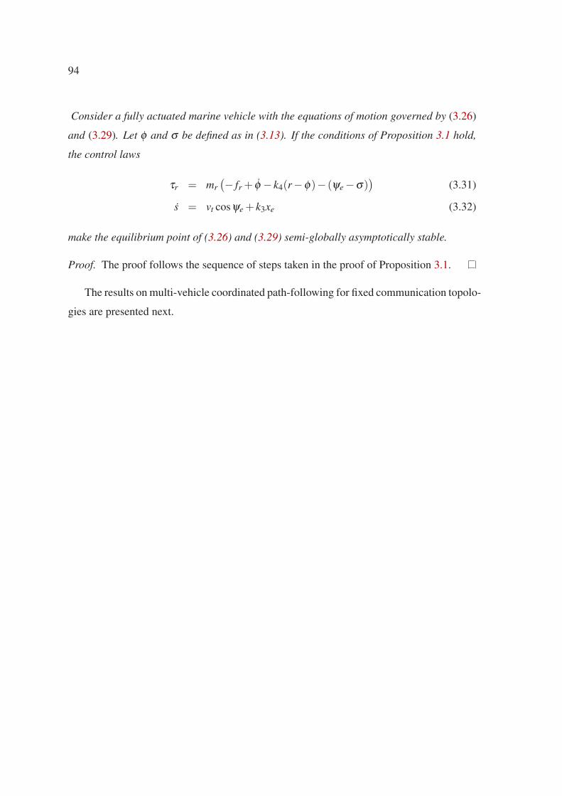
94

Consider a fully actuated marine vehicle with the equations of motion governed by (3.26)

and (3.29). Let φ and σ be defined as in (3.13). If the conditions of Proposition 3.1 hold,

the control laws

τr = mr

(

− fr + φ − k4(r−φ)− (ψe −σ))

(3.31)

s = vt cosψe + k3xe (3.32)

make the equilibrium point of (3.26) and (3.29) semi-globally asymptotically stable.

Proof. The proof follows the sequence of steps taken in the proof of Proposition 3.1.

The results on multi-vehicle coordinated path-following for fixed communication topolo-

gies are presented next.

95

3.3 Vehicle coordination control. Fixed communication

topologies

In this chapter we propose several solutions to the problem of coordinated path-following

under the restriction that the underlying communication network be fixed. Conditions are

derived under which coordination is achieved. The chapter concludes by addressing some

issues that arise in the scope of bi-directional and uni-directional communication topolo-

gies.

3.3.1 Coordination error dynamics

Equipped with the results obtained in Chapter 3.2 for the path-following problem of a single

vehicle, we now consider the problem of coordinated path-following control. In the most

general set-up, one is given a set of n ≥ 2 wheeled robots (or fully actuated marine vehicle)

and a set of n spatial paths Γk; k = 1,2, ...,n and require that robot k follow path Γk. We

further require that the vehicles move along the paths in such a way as to maintain a desired

formation pattern compatible with those paths. Recall that in the solutions given for the

path-following problem, the vehicle is driven to the “virtual target” which is parameterized

by si, the signed curvilinear abscissa on the path. Assume each vehicle is equipped with

a path-following control law, so that the evolution of the corresponding “virtual target” is

given by

si = vi cosψei + k3ixei (3.33)

as derived in (3.32), where vi denotes the total speed of the vehicle. It now remains to

coordinate (that is, synchronize) the vehicles in time so as to achieve a desired formation

pattern. As will become clear shortly, this will be achieved by adjusting the speeds of the

vehicles as functions of the “along-path” distances among them.

The dynamics of the total speed of the i’th vehicle, that is, (3.12) for a wheeled robot

and (3.29) for a marine vehicle, can be rewritten as

vi = Fi (3.34)

96

where Fi = Fi/m for a wheeled robot, and Fi = τvti+ fvti

for a marine vehicle.

Now, let each path Γi be parameterized in terms of a parameter ξi that is not necessarily

the arc length along the path. An adequate choice of the parameterization will allow for

the conclusion that the vehicles are synchronized iff ξi = ξ j for all i, j. For example, in

the case of two vehicles following two circumferences, Figure 1.5, with radii R1 and R2

while keeping an in-line formation pattern, ξi = si/Ri; i = 1,2. See Chapter 1 for more

details. Denote by si = si(ξi); i = 1,2, ...,n the corresponding arc length. We define Ri(ξi) =

∂ si/∂ξi and assume that Ri(ξi) is positive and uniformly bounded for all ξi. In particular, si

is a monotonically increasing function of ξi. We further assume that all Ri(ξi) is bounded

away from 0 and that ∂Ri/∂ξi is uniformly bounded. The symbol Ri(.) is motivated by the

nomenclature adopted before for the case of paths that are nested arcs of circumferences.

Using equation (3.33) and the fact that ξi = Risi, it is straightforward to show that the

evolution of ξi is given by

ξi =1

Ri(ξi)(vi cosψei + k3ixei) (3.35)

which can be re-written as

ξi =1

Ri(ξi)vi +di (3.36)

where

di =1

Ri(ξi)[(cosψei −1)vi + k3ixei]. (3.37)

Notice from Section 3.2 that if vehicle i tends to the assigned path di → 0 asymptotically

as t → ∞, if vi is bounded. Later in this chapter, it will be shown that this assumption is

met. Suppose one vehicle, henceforth referred to as vehicle L , is elected as a “leader”

and let the corresponding path ΓL be parameterized by its length, that is, ξL = sL . In

this case, RL (ξL ) = 1. It is important to point out that L can always be taken as a

“virtual” vehicle that is added to the set of “real” vehicles as an expedient to simplify the

coordination strategy. Let vL = vL (t) be a desired speed profile assigned to the leader

in advance, that is ξL = vL , and known to all the other vehicles. Notice now that in the

ideal steady situation where the vehicles move along their respective paths while keeping

the desired formation, we have ξi −ξL = 0 and therefore ξi = vL for all i = 1, ..,n. Thus,

97

vL becomes the desired speed of each of the vehicles, expressed in ξi coordinates. As

such, one can proceed without having to resort to the concept of an actual or virtual leader

vehicle, thus making the coordination scheme truly distributed.

From (3.36), making di = 0, it follows that the desired inertial velocities of vehicles

1 ≤ i ≤ n equal Ri(ξi)vL (t). This suggests the introduction of the speed-tracking error

vector

ηi = vi −Ri(ξi)vL , 1 ≤ i ≤ n. (3.38)

Taking into account the vehicle dynamics, (3.38) yields

ηi = ui = Fi −d

dt(Ri(ξi)vL ) . (3.39)

Using (3.36), it is also easy to compute the dynamics of the origin of each Serret-Ferret

frame Ti as

ξi = 1Ri

ηi + vL +di. (3.40)

To write the above dynamic equations in vector form, define η = [ηi]n×1, ξ = [ξi]n×1,

u = [ui]n×1, d = [di]n×1 and C = C(ξ ) = diag[1/Ri(ξi)]n×n to obtain

η = u

ξ = Cη + vL 1+d(3.41)

where 1 = [1]n×1. In the above, matrix C is positive definite and bounded, that is,

0 < c1I ≤C(ξ (t)) ≤ c2I (3.42)

for all t, where c1 and c2 are positive scalars and I the identity matrix. Notice that C

is allowed to be (state-driven) time-varying, thus allowing for more complex formation

patterns than those in the motivating examples of Chapter 1. We will present an example

for coordinated path-following with varying C, later in Section 3.4.

The objective is to derive a control strategy for u to make ξ1 = ... = ξn or, equiva-

lently, (ξi − ξ j) = 0 for all i, j. The first type of constraints is imposed by the types of

links available for communication. The second type of constraints arises from the need to

drastically reduce the amount of information that is exchanged over the communications

98

network. It will be assumed that the vehicles only exchange information on their positions

and speeds. We will derive several solutions to the problem of the vehicles coordination

with bi-directional and uni-directional communication.

Remark 3.8. Since the coordination states are non-dimensional variables, one can always

normalize them, that is, make ξ ′i = kξi for some k > 0. Consequently, R′

i = ∂ si/∂ξ ′i =

∂ si/(k∂ξi) = Ri/k and C′ = kC. This is particularly helpful when the paths are concate-

nation of sub-paths of different types (straight lines, nested arcs, etc.). Using different

normalization gains for each part, it is possible to bring all the parametrization variables to

the same range.

3.3.2 Bi-directional communications

We now comment on the type of communication constraints contemplated in this section.

It is assumed that i) the communications are bi-directional, that is, if vehicle i sends in-

formation to j, then j also sends information to i. Formally that is j ∈ Ni iff i ∈ N j, and

ii) the communications graph is connected. Notice that if assumption (ii) is not verified,

then there are two or more clusters of vehicles and no information is exchanged among the

clusters. Clearly, in this situation no coordination is possible.

Definition 3.3 (Coordination control)

Consider the vehicle coordination system with dynamics (3.41) where C satisfies the

bounds in (3.42), vL is the desired formation speed, and d tends asymptotically to zero.

Further assume that each of the n vehicles has access to its own state and exchanges infor-

mation on its path parameter (coordination state) ξi and speed tracking error ηi with some

or all of the other vehicles defined by neighboring sets Ni. Determine a feedback control

law for u such that limt→∞ ηi = 0 and limt→∞(ξi −ξ j) = 0 for all i, j = 1, ..,n.

In the sequel, three solutions are presented for coordination control problem above: i)

Proposition 3.4 offers two solutions with linear control laws, and ii) Proposition 3.5 gives a

version of one of the solutions in i with a nonlinear control law which employs a saturation

function.

Coordination problem solutions

99

The next proposition offers two solutions to coordination problem Definition 3.3, under the

basic assumption that the communications graph G is bi-directional and connected.

Proposition 3.4 (Solution I & II. Linear control laws)

Consider the coordination problem defined in 3.3 with d = 0 and assume that the underly-

ing communications graph G (defined by sets Ni) is connected. Let L be the Laplacian of G ,

and A = diag[ai]n×n and B = diag[bi]n×n be arbitrary positive definite diagonal matrices.

Then, the control laws

Solution I

u = −(LC +C +A)η −ALξ (3.43)

Solution II

u = −Aη −BCLξ , (3.44)

solve the coordination problem. Namely, the control laws meet the communication con-

straints and the origin is a uniformly globally exponentially stable (UGES) equilibrium

point of the coordination closed-loop subsystem.

Proof. The proof is given later in this section.

When using the term stability of the equilibrium of the coordination system, we refer to

the stability of ηi = 0,ξi −ξ j = 0;∀i, j = 1, ...,n. The following proposition offers another

solution to the coordination problem in Definition 3.3. The control law is a version of (3.43)

with a saturation function that adds an extra option for the designer to keep the speeds of

the vehicles in a bounded region. Recall that the disturbance-like term d tends to zero if

v(t) is bounded. Thus, boundedness of v(t) simplifies the proof of stability of the system

resulting from putting together the path-following and the coordination subsystems.

Proposition 3.5 (Solution III. With saturation function)

Consider the coordination problem described in Definition 3.3 and assume that the com-

munications graph G is connected and d = 0. Let L be the Laplacian of G , and A =

diag[ai]n×n and B = diag[bi]n×n be arbitrary positive definite diagonal matrices. Then, the

100

control law

u = −(A−1L+A)Cη −Bsat(η +A−1Lξ ), (3.45)

where sat is the saturation function

sat(x) =

xm x > xm

x |x| ≤ xm

−xm x < −xm

(3.46)

with xm > 0 arbitrary, solves the coordination problem. Namely, the control law meets

the communication constraints and the origin is a uniformly globally asymptotically stable

(UGAS) equilibrium point of the coordination closed-loop subsystem.

Proof. The proof is given later in this section.

Remark 3.9. The assumption that d tends asymptotically to 0 as t → ∞ will be justified

later in this chapter, which contains the analysis of the dynamic behavior of the combined

path-following and coordination systems.

Proofs

We start by modeling the communication network as an undirected graph G which we

assume is connected. Choose a spanning tree T of the connected graph G and associate

to G an arbitrary orientation σ . Partition the incidence matrix M of G σ as M = [M1,M2],

where M1 is the incidence matrix of T σ . As explained in Section 3.1.2, the graph Laplacian

can be written as L = M1Y 2MT

1 for some Y > 0, where M1 is of order n×n−1, RankM1 =

n−1, MT

1 M1 is invertible, and M11 = 0. Introduce formally the graph-induced coordination

error as

θ := Y MT

1 ξ . (3.47)

Notice that θ ∈Rn−1. From the above relation, θ = 0 is equivalent to ξi = ξ j,∀i, j. Conse-

quently, if θ is driven to zero asymptotically, so are the coordination errors ξi −ξ j and the

problem of coordinated path-following (Definition 3.3) is solved. This justifies the choice

of the error vector (3.47).

Proposition 3.4

101

Proof of Solution I. Consider the coordination dynamics (3.41) with the control law (3.43).

The closed-loop dynamics in terms of (η ,θ) ∈Rn ×R

n−1 can be represented as

η = −(M1Y 2M1C +C +A)η −AM1Y θ

θ = Y MT

1Cη +Y MT

1 d.(3.48)

Let

z = η +M1Y θ

and consider the candidate Lyapunov function

V =1

2θ T θ +

1

2zT z.

Clearly, V is positive definite and radially unbounded on (η ,θ). Computing the deriva-

tive of V along the solutions of (3.48) with d = 0 yields

V = −ηTCη − zT Az

which is negative and is zero only at equilibrium point, since M1 is full rank and Y > 0.

Therefore, V is negative definite and resorting the Lyapunov stability theorem (η ,θ) =

(0,0) is a uniformly globally exponentially stable (UGES) equilibrium point.

We now examine the form of the control law (3.43), which can be written as

ui = −(ai +1

Ri)ηi − ∑

j∈Ni

(aiξi +1

Riηi −aiξ j −

1

R jη j).

Notice how the control input of vehicle i is a function of its own speed-tracking error and

coordination state as well as of the coordination states and speed-tracking errors of the

other vehicles included in the index set Ni. Clearly, the control law is decentralized and

meets the constraints imposed by the communications network, as required.

Proof of Solution II. Consider the coordination dynamics (3.41) with the control law (3.44).

The closed-loop dynamics in terms of (η ,θ) can be written as

η = −Aη −BCM1Y θ

θ = Y MT

1Cη +Y MT

1 d.(3.49)

102

In what follows, we show that for d = 0 the functions V and W defined as

V = 12ηT B−1η + 1

2θ T θ

W = ηT M1Y θ .(3.50)

satisfy the conditions of Matrosov theorem (see page 70), thus proving that the origin is a

UGES equilibrium point for the dynamic equations (3.49).

Let x := (ηT ,θ T)T and define Ω := x ∈ Rn ×R

n−1 : ‖x‖ ≤ α. It is easy to see that

conditions 1, 3, and 5 of Matrosov’s theorem (on page 70) are indeed satisfied for any

(η ,θ) ∈ Ω and for some c1,c2 > 0 and α1,α2 ∈ classK . Computing the derivative of V

along the solutions of (3.49) yields V = −ηT B−1Aη , which fulfills condition 2. It remains

to show that condition 4 is satisfied for some α3 ∈ classK . To this effect, start by defining

E = x ∈ Ω : V = 0 = (0T ,θ T)T ∈ Ω and compute the distance of point x to E as

dist(x,E) = ‖η‖ =√

ηT η . (3.51)

Compute also the derivative of W to obtain

W = −ηT AM1Y θ −θ TY MT

1CBM1Y θ +ηT M1Y 2MT

1Cη

= −xT Qx+ηT(P+M1Y 2MT

1C)η(3.52)

where

Q =

(

P 12AM1Y

12Y MT

1 A Y MT

1CBM1Y

)

(3.53)

with an arbitrary P. Now, to make Q > 0, let P = ρ4c1

B−1A2 for some ρ > 1, where c1 is the

uniform lower bound of C(t) in (3.42). This can be shown by taking Schur complements

as follows. Since P > 0, then Q > 0 if

Y MT

1CBM1Y − 14Y MT

1 AP−1AM1Y = Y MT

1 (CB− 14A2P−1)M1Y

= Y MT

1 B(C− c1ρ I)M1Y > 0

where we used the fact that C− c1ρ I > 0. Define P1 = P + 1

2(LC +CL), and rewrite (3.52)

as

W = −xT Qx+ηT P1η . (3.54)

103

It can be shown that P1 > 0 for large enough ρ . The proof is identical to that of

Lemma 6.1, since P and C are positive definite diagonal matrices. Then, we have

p1ηT η ≤ ηT P1η ≤ p2ηT η

q1xT x ≤ xT Qx ≤ q2xT x(3.55)

for some positive scalars p1, p2,q1,q2. Since ‖x‖= (ηT η +θ T θ)1/2 < α for all x ∈ Ω, then

1

αηT η ≤

√

ηT η ≤ α (3.56)

and finally

max(√

ηT η , |W |) ≥ max(1

αηT η , |W |). (3.57)

Therefore, to prove that condition 4 of the Matrosov theorem is satisfied, it is sufficient to

show that max( 1α ηT η , |W |) ≥ α3(||x||) for some α3(.) ∈ classK . This is done next.

Choose β such that 0 < β < min(1,α p2). Obviously, β < 1 and β/(α p2) < 1. We

consider two different possibilities: i) W ≥ 0 and ii) W < 0.

i) Suppose W ≥ 0. From (3.54), ηT P1η ≥ xT Qx and therefore

xT Qx ≤ p2ηT η ⇒ 1

α p2xT Qx ≤ 1

αηT η . (3.58)

Simple algebra shows that

max(dist(x,E),W ) ≥ max(

1α ηT η ,ηT P1η − xT Qx

)

= max(

1α ηT η , 1

α p2xT Qx,ηT P1η − xT Qx

)

≥ max(

1α ηT η , 1

α p2xT Qx, β

α p2(ηT P1η − xT Qx)

)

≥ 13

(

1α ηT η + 1

α p2xT Qx+ β

α p2(ηT P1η − xT Qx)

)

≥ 13

(

( 1α + β p1

α p2)ηT η + (1−β )q1

α p2xT x)

≥ λ1xT x

(3.59)

where λ1 = (1−β )q1

3α p2and we used the properties of max(., .) listed in Section 3.1.1.

104

ii) Suppose W ≤ 0. From (3.54), ηT P1η ≤ xT Qx, and therefore

max(dist(x,E),−W ) ≥ max(

1α ηT η ,xT Qx−ηT P1η

)

≥ max(

1α ηT η , β

α p2(xT Qx−ηT P1η)

)

≥ 12

(

1α ηT η + β

α p2(xT Qx−ηT P1η)

)

≥ 12

(

1−βα ηT η + βq1

α p2xT x)

≥ λ2xT x

(3.60)

where λ2 = βq1

2α p2.

Let λ = min(λ1,λ2) and define α3(‖x‖) = λxT x, which is of classK . Results i) and ii)

above show that max(dist(x,E), |W |) ≥ α3(||x||), thus showing that the origin is a UGAS,

therefore UGES equilibrium point, since the dynamics are linear.

Remark 3.10. Consider the coordination dynamics (3.41) with the linear control law

u = −Aη −BCMWMT

where A = diag[ai], B = diag[bi] and W = diag[wi] are positive diagonal matrices, and M is

the incidence matric of the communication graph, that is, the graph Laplacian L = MMT .

We further assume that matrix C = C(ξ ) is constant. While restrictive, this still allows

one to consider paths that consist of translations of straight lines, nested circumferences,

and parallel translations of one arbitrary path. Define the graph-induced coordination error

θ = MT ξ and compute the closed-loop dynamics in terms of η and θ as

η = −Aη −BCMθ

θ = MTCη

for d = 0. Let

V =1

2ηT B−1η +

1

2θ TWθ (3.61)

be the candidate Lyapunov function whose time derivative along the solutions of the closed-

loop dynamics is V =−ηT B−1Aη , which is negative semi-definite. Note that V = 0 ⇒ η =

0 which in turn implies that Mθ = 0. Moreover, Mθ = 0 ⇒ Lξ = 0 ⇒ ξ ∈ span1⇒ θ =

MT ξ = 0. Since the system is time-invariant and V is radially unbounded, a straightforward

105

application of LaSalle’s invariance principle shows that the origin is UGES. Let k = e(i, j)

mean that edge Vi,V j is the k− th element in the ordered list of edges. Close examination

of the control law reveals that it can be written in a decentralized form as

ui = −aiηi −bi

Ri(ξi)∑

j ∈ Ni

k = e(i, j)

wk(ξi −ξ j) (3.62)

Notice that vehicle i only has access to its speed and the coordination state, and to the

coordination states ξ j of its neighbors. Making W identity, the abovementioned control law

degenerates to (3.44).

Proposition 3.5

Proof of the coordination control law with sat(.) With the control law (3.45), the dynamics

of the coordination system (3.41) can be written in terms of η and θ as

η = −(A−1M1Y 2MT

1 +A)Cη −Bsat(η +A−1M1Y θ),

θ = Y MT

1Cη +Y MT

1 d,(3.63)

where we used the fact that MT

1 vL 1 = 0. Let

z = η +A−1M1Y θ

and consider the candidate Lyapunov function

V =1

2θ T θ +

1

2zT z.

Clearly, V is positive definite and radially unbounded on (η ,θ). Computing the deriva-

tive of V along the solutions of (3.63) with d = 0 yields

V = −ηT ACη − zT Bsat(z).

which is negative definite with respect to (ηT ,zT)T = 0, or equivalently with respect to

(ηT ,θ T)T = 0, since M1 is full rank and Y > 0. Therefore the origin is a UGAS equilibrium

point of (3.63). The control law (3.45) in a decentralized form can be written as

ui = − ai

Riηi −

1

ai∑j∈Ni

(1

Riηi −

1

R jη j)−bi sat

(

ηi +1

ai∑j∈Ni

(ξi −ξ j)

)

. (3.64)

106

Notice that the control signal of vehicle i is a function of its own speed and coordination

state as well as of the coordination states and speeds of the other vehicles defined by Ni.

Clearly, the control law is decentralized and meets the constraints imposed by the commu-

nications network, as required.

3.3.3 Time-varying pattern tracking

In Chapter 1, with the help of simple motivating examples, we showed how the problem of

coordinated path-following can be essentially reduced to that of “aligning” the coordina-

tion states ξi asymptotically, that is, making ξi −ξ j → 0 for all i and j as t → ∞. Further, it

was also shown how the coordination ξi state of each vehicle yields a re-parametrization of

its assigned path as a function of path length si, that is, ξi = ξi(si). Using this set-up, for-

mation patterns (compatible with the paths being followed) are obtained by proper choice

of the parametrization functions ξi(s), which must be computed in advance. In the case of

complex but fixed formation patterns that are path-dependent, the re-parametrization can

be done but may assume a complicated form. This problem is further aggravated in the

case of desired formation patterns that are explicit functions of time, because in this case

the above re-parametrization is simply non-existent. This section offers a methodology for

time-varying pattern tracking that is simple to implement and overcomes the above prob-

lems. The rationale behind the methodology can be explained by referring to the simple

case of a number of vehicles doing coordinated path-following along parallel straight lines.

With ξi = si and the methods proposed so far, coordination is achieved when the vehicles

assume an in-line formation pattern, which will henceforth be called the baseline pattern

or configuration. Now, it is easy to go from the baseline configuration to a more complex,

possibly time-varying formation, by introducing appropriate offsets in the desired positions

of the vehicles with respect to the position of a fictitious Leader or with respect to the aver-

age point of the formation. We take the latter approach and formalize it as follows. Recall

the coordination dynamics

η = u

ξ = Cη + vL 1+d(3.65)

107

and assume as before, at this stage, that d = 0. Define α (the average point of the formation)

and δ (the offset of the vehicles with respect to α) as

α :=1

n1T ξ (3.66)

and

δ := ξ −α1, (3.67)

respectively and notice that 1T δ = 0. Define now the (pattern-induced) reference vector h(t)

with respect to α , which satisfies necessarily the relation 1T h(t) = 0. Then, the problem of

time-varying pattern tracking is reduced to that of making (δ −h) → 0 as t → ∞.

With the change of variables

µ = η −C−1h

θ = Y MT

1 (ξ −h)

u0 = ddt

(C−1h),

(3.68)

the dynamics of (µ,θ) are given by

µ = u−u0

θ = Y MT

1Cµ(3.69)

The methodology used in the last section can now be exploited to show that the coordination

control law u = u0 − (A−1M1Y 2MT

1 +A)Cµ − Bsat(µ +A−1M1Y θ) or, equivalently (in the

original state-space) the control law

u =d

dt(C−1h)− (A−1L+A)(Cη − h)− Bsat(η −C−1h+A−1L(ξ −h)) (3.70)

renders the origin of the closed-loop system uniformly globally asymptotically stable (UGAS).

As a consequence, as t →∞, θ → 0. Therefore, using the fact that MT

1 1 = 0, MT

1 (ξ −h)→ 0

implies that MT

1 (δ −h) → 0. Because 1T δ = 0 and 1T h = 0, that is, δ −h is normal to the

null space of MT

1 , we conclude that (δ −h)→ 0 as required. In the exposition above, it was

implicitly assumed that the reference h(t) is sufficiently smooth in order for its derivatives

to exist.

The above control law can be written in decentralized form as

108

ui =d

dt(Rihi)−ai(

1

Ri

ηi − hi)−1

ai∑j∈Ni

(1

Ri

ηi − hi −1

R j

η j + h j)

−bi sat(ηi −Rihi +1

ai∑j∈Ni

(ξi −hi −ξ j +h j)).

Notice that vehicle i needs to know the difference ξ j − h j between the coordination

variable ξ j and reference h j of vehicle j (but not the coordination state ξ j itself) together

with 1R j

η j − h j.

Remark 3.11. The offset h(t) can always be given with respect to any convenient reference

point. It is a simple matter to compute the average of h and subtract the average from h

to make the condition 1T h = 0 hold. That is, the new h is computed as h − (1T hn

)1 =

(I − 1n11T)h.

3.3.4 Uni-directional communications

In this section, we study the stability of the coordination dynamics under the assumption

that the communications among the vehicles are uni-directional. Moreover, we will assume

that the coordination dynamics (3.41) are time-invariant, that is, the matrix C(ξ ) is constant.

While restrictive, this assumption still allows one to consider paths that consist of straight

lines, nested circumferences, and parallel translations of one arbitrary path.

Let G denote the graph that represents the communication network among the vehicles

and L the associated Laplacian matrix. Moreover, assume that G has a globally reachable

vertex. In this case, L can be decomposed as in (3.6), that is, L = F1L11F2. Define θ =

F2ξ ∈Rn−1. The coordination dynamics (3.41) can be written in terms of η and θ as

η = u

θ = F2Cη +F2d,(3.71)

using the fact that F21 = 0. Moreover, since RankF2 = n− 1, then θ = 0 ⇔ ξi = ξ j for

all i, j. Consequently, if θ is driven to zero asymptotically, so are the coordination errors

ξi −ξ j and the problem of coordinated path-following is solved. This key observation sets

the stage for the mathematical formulation of the coordinated control problem that follows.

109

In this section, we will give solutions to the vehicle coordination problem as stated in

Definition 3.3 with constant matrix C and uni-directional communication topologies.

Coordination control solution

The main result of this section is stated below.

Proposition 3.6 (Coordination, Directed graph)

Consider the coordination dynamics (3.41) with constant matrix C. The control law

u = −Aη −BC−1Lξ , (3.72)

solves the coordination problem for positive definite scalar matrices A = aI and B = bI if

the graph G (L) has at least one globally reachable vertex and

a2

b> max

µ∈σ(L)−0

Im(µ)2

Re(µ)(3.73)

where σ(.) stands for the spectrum of a matrix and Im(.) and Re(.) denote the imaginary

and real part of a complex number. Furthermore, the control law (3.72) can be written in

decentralized form as

ui = −aηi −bRi(ξi) ∑j∈Ni

(ξi −ξ j) (3.74)

Proof. Consider for the time being the case where d = 0 (this assumption will be lifted

later). The unforced closed-loop coordination system consisting of equations (3.71)-(3.72)

can be written as

η = −Aη −BC−1F1L11θ

θ = F2Cη(3.75)

We now show that the closed-loop matrix

Acl =

(

−A −BC−1F1L11

F2C 0

)

is a stability (Hurwitz) matrix, thus proving that the linear system (3.75) is uniformly glob-

ally exponentially stable (UGES). To this effect, we start by computing the eigenvalues of

110

Acl as functions of the eigenvalues of L11. Simple computations show that

σ(Acl) = σ(

(

F−1B−1C 0

0 I

)

Acl

(

C−1BF 0

0 I

)

)

= σ(

−aIn −(

β T

F2

)

F1L11

bF2

(

1 F1

)

0

)

= σ(

−aIn −(

0T

In−1

)

L11

b(

0 In−1

)

0

),

(3.76)

and therefore σ(Acl) = σ(Acl1), where

Acl1 =

−a 0T 0T

0 −aIn−1 −L11

0 bIn−1 0

(3.77)

where 0 denotes a square matrix of zeros. It is easily seen that λ = −a is an eigenvalue of

Acl1 and thus of Acl . The rest of the eigenvalues are given by the roots of

det(

(

(λ +a)In−1 +L11

−bIn−1 λ In−1

)

) = 0. (3.78)

At this point, use the Lemma that for any matrices A, B, C and D with proper dimensions

det(

(

A B

C D

)

) = det(AD−BC),

if CD = DC. Applying the Lemma, (3.78) can be simplified to

det(λ (λ +a)I +bL11) = 0. (3.79)

Let µ ∈ σ(L11) be an arbitrary eigenvalue of L11, recall that Re(µ) > 0 . From (3.79),

it follows that

µ = −λ (λ +a)

b. (3.80)

111

Clearly, to every µ there correspond two possible values for λ given by

λ1,2(µ) = −√

b(c±√

c2 −µ) (3.81)

where c = 0.5a/√

b. Let µ = µr + µi

√−1 with µr > 0. Then, the real parts of the corre-

sponding eigenvalues λ1,2(µ) are negative if

a2

b> max

µ∈σ(L11)

µ2i

µr. (3.82)

The technical condition (3.73) in the statement of the theorem follows immediately

from the fact that σ(L) = σ(L11)∪0.

Remark 3.12. Notice that the eigenvalues of the closed-loop coordination system given

in (3.81) are independent of the matrix C. A similar result was derived in Chapter 2 for

communication links with a simple structure, using linearization techniques. This result

is therefore a non-trivial extension of the results in Chapter 2 to a nonlinear setting and to

more realistic communication structures.

Remark 3.13. Notice that the coordination control law

u = −Aη −BCLξ . (3.83)

is the same as (3.44) derived for the case of undirected graphs but differs from

u = −Aη −BC−1Lξ (3.84)

derived for the case of directed graphs in (3.72). The stability condition for the closed-loop

system resulting from (3.65) with control (3.83) changes to

a2

b> max

06=µ∈σ(L)

Im(µ)2

Re(µ)c2, (3.85)

where C = cI. Notice that the stability condition is no longer independent of matrix C.

Remark 3.14. The stability condition (3.85) does not contradict Proposition 3.4 where

we have shown that the closed-loop coordination dynamics are stable for any diagonal

matrix A and B. The argument is as follows. The eigenvalues of the graph Laplacian L are

112

all real numbers if the graph is symmetric, for example in the case of undirected graphs.

Considering the fact that the condition (3.85) is always true for any positive a and b, if all

the eigenvalues of L are real, the statement of the proposition is verified.

Remark 3.15. The pattern tracking algorithm derived in Section 3.3.3 can be extended to

the case of uni-directional communications. However, the results can only be guaranteed

for time-invariant systems and therefore apply to fixed formation patterns. Let the constant

vector h be the desired reference pattern defined with respect to the middle point of the

formation, that is, 1T h = 0. Using arguments similar to those in Section 3.3.3, it can be

shown that the control law

u = −Aη −BC−1L(ξ −h) (3.86)

solves the coordination problem and that the vehicles exponentially converge to the desired

pattern defined by h, that is, limt→∞(ξi −hi)− (ξ j −h j) = 0; ∀i, j.

3.3.5 Truly decentralized vehicle coordination

In all the solutions derived so far to the coordinated path-following control problem, we

assumed that a predefined velocity profile vL is known to all vehicles. This is apparent in

the coordination dynamics of (3.41), where the speed error is defined as ηi = vi−RivL . In

many situations, however it is natural to assume that the “pace of the fleet” is set during the

mission by one of the members, namely the Leader.

In order to make the coordination algorithms truly decentralized, this section derives

a strategy that keeps the amount of required information flow as low as before, while vL

is known only to one of the vehicles. With the structure proposed, the only vehicle who

knows the value of vL (actually the one that sets its value) is a globally reachable vertex in

the underlying communication graph. We further assume that vL is constant and present

the solution for general digraphs. An undirected graph will be modeled by its equivalent

symmetric digraph, that is, a digraph with two arcs in opposite directions for each edge of

the undirected graph.

Consider the coordination problem of n vehicles supported by a communication net-

work. Let the underlying graph Gn have at least one globally reachable vertex which will

113

GR-vertex

Virtual Leader

Fleet

Figure 3.5: Augmented graph. vL known only to the virtual leader

be called GR-vertex. Number the vertices of Gn in increasing order as 2, ...,n + 1 and

assume without loss of generality that V2 is a GR-vertex. Add a vertex numbered 1 to

V (Gn), where V1 is a virtual vehicle moving at constant speed vL . Construct the graph

Gn+1 by adding an arc namely arc (V2,V1), that captures the transmission of information

from V1 (virtual leader) to V2 (GR-vertex), see Figure 3.5. Notice that vertex V1 in Gn+1

is the only GR-vertex: it is globally reachable because it is reachable from V2 while V2 is

reachable from every other node but V1, and it is unique since none of the other vertices

can be reached from V1. Therefore, Gn+1 has a GR-vertex. The Laplacian matrix of Gn+1

has the structure

L =

(

0 0T

−e1 Ln

)

(3.87)

where e1 = [1,0, ...,0]T and Ln is a n×n matrix. That is, the first row of L that corresponds

to the “virtual leader” is zero.

Let D and A be the out-degree and adjacency matrices of graph Gn+1, respectively,

modified as follows: set the 11−entries of D and A to 1. With this modification, the new

D is invertible 4 and L = D−A does not change. Define a normalized version of the graph

4Every other vertex has at least out-degree equal 1, since V1 is the only globally reachable vertex.

114

Laplacian as L = D−1L = I −D−1A. Further define

ξ = D−1Aξ ⇔ ξi =

1|Ni| ∑ j∈Ni

ξ j, |Ni| 6= 0

ξi, |Ni| = 0, (3.88)

where ξ is the vector of coordination states of graph Gn+1. Notice that since |Ni| is the

number of the neighbors of Vi, then ξi is the average of the coordination states of its neigh-

bors.

We now rewrite a version of the coordination closed-loop dynamics with system dy-

namics (3.34), (3.36) and the control law (3.72), for constant vL and a constant matrix C,

in terms of the states v and ξ , as follows

v = F

ξ = Cv+d(3.89)

with the control law

F = −a(v−C−1vL 1)−bC−1Lξ ,

where a,b > 0 satisfy condition (3.73), and L is the graph Laplacian of Gn+1. The argu-

ments of Proposition 3.6 apply to (3.89). Thus, for d = 0, at steady-state vi = RivL and

ξi = vL and therefore the average of the derivative of any subset of the coordination states,

namely Ni, is vL , that is,˙ξi = vL ;∀i. This suggests to feedback

˙ξi (or any estimate of it)

instead of vL , that is, to apply the control law

F = −a(v−C−1 ˙ξ )−bC−1Lξ . (3.90)

Notice that L and L coincide at the nonzero entries, therefore using L instead of L only

changes the gains and not the communication constraints (the details will be shown later).

Simple manipulations yield the dynamics

˙ξ = D−1Aξ = D−1ACv.

Therefore, F derived in (3.90) can be written in terms of the states (ξ ,v) as F =−aC−1LCv−bC−1Lξ . This justifies the choice of control law that will be given next.

115

Notice that all the vectors in (3.89) have dimension n + 1 with compatible matrices,

where the first rows belong to the “virtual leader”, that is

v1 = vL

ξ1 = ξL

f1 = 0

R1 = 1, (11-entry of C)

d1 = 0.

(3.91)

The above introduction motivates the following proposition.

Proposition 3.7 (Truly decentralized coordination control)

The control law

F = −aC−1LCv−bC−1Lξ , (3.92)

where L is the (normalized) graph Laplacian of Gn+1 , stabilizes the coordination dynamics

(3.89) for constant vL and constant C if

a2

b> max

µ∈σ(L)−0

µ2i

µr(µ2r + µ2

i ), (3.93)

where µr = Re(µ) and µi = Im(µ) and at steady-state vi = RivL and ξi = ξ j ∀i, j =

1, ...,n+1. Furthermore, (3.92) meets the communication constraints.

Proof. Since L has a globally reachable vertex, it can be decomposed as in (3.6) where

L = F1L11F2. Define the error vector θ = F2ξ . Since RankF2 = n, θ = 0 ⇔ ξi = ξ j∀i, j.

The closed-loop dynamics in terms of v and θ , for d = 0, are given by

v = −aC−1F1L11F2Cv−bC−1F1L11θ

θ = F2Cv.(3.94)

We proceed in three steps to verify that i) θ = 0 and vi = RivL ;∀i is an equilibrium point

of the closed-loop coordination system, ii) the control laws are in decentralized form, and

iii) the control laws render the closed-loop system asymptotically stable, that is, stability

and convergence of the solutions to the equilibrium are observed.

i) Equilibrium point. From the first row of (3.94) or (3.92) we have that v1 = 0. Thus,

it is enough to choose the initial condition v1(0) = vL to guarantee that v1(t) = vL . At

116

equilibrium θeq = 0 and therefore F2Cveq = 0 or equivalently Cveq = vo1 for some vo ∈R;

the first row of these equations shows that vo = vL . Substituting veq = C−1vL 1 in the first

equation of (3.94) results in C−1F1L11θeq = 0. Then, multiplying on the left by L−111 F2C

yields θeq = 0.

ii) Decentralized control law. The control law given in (3.92) in a decentralized form

can be written as

Fi = −aRi ∑ j∈Ni( 1

Rivi − 1

R jv j)−bRi ∑ j∈Ni

(ξi −ξ j)

= −a|Ni|vi −b|Ni|Riξi +Ri ∑ j∈Nia

v j

R j+bξ j,

for vehicle i. If we substitute L by L = I −D−1A in the control law, then the control signal

becomes

Fi = −avi −bRiξi +Ri

|Ni| ∑j∈Ni

av j

R j

+bξ j.

Notice that Fi = |Ni|Fi.

iii) Stability and convergence. We now show that under condition (3.93), the eigenval-

ues of the closed-loop matrix

Acl =

(

−aC−1F1L11F2C −bC−1F1L11

F2C 0

)

are on the left-half-plane, except one eigenvalue at zero which corresponds to v1 = 0, thus

proving that equilibrium θeq = 0 and veq−C−1vL 1 = 0 of the linear system (3.94) is UGES.

We start by computing the eigenvalues of Acl as functions of the eigenvalues of L11. Simple

computations show that

σ(Acl) = σ(

(

F−1C 0

0 I

)

Acl

(

C−1F 0

0 I

)

)

= σ(

−a

(

0 0T

0 L11

)

−b

(

β T

F2

)

F1L11

F2

(

1 F1

)

0

),

and therefore σ(Acl) = σ(Acl1), where

Acl1 =

0 0T 0T

0 −aL11 −bL11

0 In 0

(3.95)

117

Clearly, Acl1 has one eigenvalue at 0 which corresponds to v1 = 0, the virtual leader’s

dynamic. The rest of the eigenvalues are the roots of

det(

(

λ In +aL11 bL11

−In λ In

)

) = 0.

At this point, use the Lemma that for any square matrices A, B, C and D

det(

(

A B

C D

)

) = det(AD−BC),

if CD = DC. Applying the Lemma, the characteristics polynomial of Acl is simplified to

det(λ 2In +(aλ +b)L11). Therefore if µ ∈ σ(L11), then

µ =−λ 2

aλ +b.

Knowing that Re(µ) > 0, after some algebra, it can be shown that the roots of λ 2 +aµλ +

bµ = 0 have negative real part if

a2

b> max

µ∈σ(L11)

µ2i

µr(µ2i + µ2

r ). (3.96)

and the results follow.

Remark 3.16. Notice that because of the way the graph Gn+1 was constructed, L is not

symmetric. Thus, L11 has some non-real eigenvalues, that is, ∃µ ∈ σ(L11) : µi 6= 0. On the

other hand, since µr > 0, the right-hand side of (3.96) cannot be zero or infinity. That is,

the inequality has always a positive bounded right-hand side.

3.3.6 Path-following and coordination control interconnection

This section examines the behavior of the coordinated path-following system that results

from putting together the path-following control and the coordination control systems pre-

sented in the previous sections. In particular, we show that the trajectories of the relevant

state variables tend asymptotically to 0.

Recall how the two subsystems are connected via d and v in the equations of motions

(3.11) and (3.41). Proposition 3.1 showed that the origin is a globally asymptotically sta-

ble equilibrium of path-following subsystem, under some mild technical assumptions. In

particular, either of the following conditions was required

118

C.1 the speed vi(t) is uniformly continuous and limt→0 vi(t) 6= 0, or

C.2∫ ∞

t0min(k, |vi(t)|)dt = ∞.

Under these conditions, the disturbance-like term di that appears at the coordination level

was shown to vanish asymptotically to zero if

C.3 the speed vi is bounded,

thus making the states of the coordination system tend asymptotically to zero. It follows

from these considerations that Xp := [Xpi]n×1 (Xpi is the state of path-following subsystem i)

and Xc (the states of the coordination control subsystem) in Figure 3.6 tend asymptotically

to zero if the speed v satisfies C.1 ∧ C.3 or C.2 ∧ C.3. These results are formally applied

in the proofs of the propositions that contained in the present section.

We proposed three different solutions in Section 3.2 to the problem of path-following

for wheeled robots (Propositions 3.1 and 3.2) and fully actuated marine vehicles (Proposi-

tion 3.3). Moreover, in the previous chapters, several coordination control strategies were

derived. Thus, different combinations of path-following and coordination control strategies

are possible. We will group these combinations into two categories, based on the proof of

convergence of the resulting coordinated path-following system, and present key results in

Propositions 3.8 and 3.9. This approach is summarized in Table 3.1 that shows how the

coordination control strategies are classified in two general control laws: i) Linear and ii)

with a sat(.) function.

In Proposition 3.8, it is more natural to address the problem using C.1, while the proof

of Proposition 3.9 is easier referring to C.2, as will become clear shortly. Since the proofs

are identical in every combination in each group, we will present statements of only repre-

sentative members.

Proposition 3.8 (Coordinated path-following I)

Consider a fleet of n wheeled robots, each equipped with the path-following control law of

Proposition 3.1. Let the corresponding coordination system be based on a bi-directional

communication network and use the control law (3.45). Let Xpi = (xei,yei,ψei)T denote the

state of the path-following subsystem of vehicle i; 1 ≤ i ≤ n . Further let Xc = (ηT ,θ T )T be

119

d

v

Xp

Xc

P.F.

C.C.

Figure 3.6: Closed-loop system consisting of the path-following and coordination control

subsystems

Path-following

Prop. 3.1 Prop. 3.2 Prop. 3.3

Coordination controlLinear Prop. 3.9 Prop. 3.9 ×Sat(.) Prop. 3.8 Prop. 3.8 Prop. 3.8

Table 3.1: Path-following and coordination: a summary of results

the relevant state of the coordination subsystem. Suppose matrix A > 0 in the coordination

control law (3.45) satisfies the constraint

a21 >

1

2(c2

c1− a1

a2)max

i|Ni| (3.97)

where a1I ≤ A ≤ a2I, and c1 and c2 are as defined in (3.42). Then, given any initial

state Xpi(0); 1 ≤ i ≤ n and Xc(0), the resulting trajectories Xpi(t) and Xc(t) are driven

asymptotically to 0.

Proof. The closed-loop system consisting of the Path-Following (PF) and Coordination

Control (CC) subsystems of Proposition 3.1 and control law (3.45), respectively are de-

picted in Figure 3.6.

Define Vη = ηT η and compute its derivative along the solutions of the coordination

subsystem (3.63) to obtain

Vη = −ηTCQCη −2ηT Bsat(η +A−1M1Y θ)

where Q =C−1A−1L+LC−1A−1 +2C−1A. From Lemma 6.1, and because C(t) is diagonal

and has a positive uniform lower bound c1, it follows from condition (3.97) that there exists

120

γ = γc21 > 0 such that ηTCQCη ≥ γ‖η‖2 and therefore

Vη ≤−γ‖η‖2 +2b2xm

√n‖η‖,

where b2I ≥ B, and xm is the limit of sat(.). Clearly, Vη is negative if ‖η‖ > 2b2xm

√n/γ .

Therefore, η is uniformly ultimately bounded and so is v(t) = η + vL C−11. See Khalil

(2002) for the definition of ultimate boundedness, together with related results of interest.

From the form of the closed-loop dynamics (3.63) it follows that η is bounded and therefore

v is also bounded. As a consequence, v(t) is uniformly continuous.

It is now necessary to show that limt→∞ vi(t) 6= 0 for all i. Assume by contradiction that

∃ j such that v j(t) = 0 for all t > t0 ≥ 0 and limt→∞ vi(t) 6= 0 ∀i 6= j (the analysis for the case

where v j tends to 0 but is not identically 0 after a certain finite time can be done identically).

Recall from the proof of Proposition 3.2 that all xei’s converge to zero as t → ∞ even if vi(t)

tends to 0. Thus, d j = 1R j

[(cosψe j − 1)v j + k3xe j]|v j=0 is also bounded and tends to zero.

Furthermore, according to Proposition 3.1, the states Xpi ∀i 6= j are bounded and converge

to zero and so do the di; ∀i 6= j. Since η and d are bounded, so is θ . Therefore θ is bounded

in any bounded interval of time. It is easy to check that (3.63) is small-signal L∞ stable

with d as an input, that is, ∃r > 0 such that if ‖d‖ < r the states remain bounded. Because

‖d‖→ 0, as t → ∞, then ∃T > 0 : ∀t > T,‖d(t)‖ < r. Therefore the states remain bounded

and decay to zero as d → 0, namely the coordination states Xc vanish asymptotically. Thus,

η = v− vL C−11 and in particular η j = v j −R jvL converge to 0, which contradicts the

assumption that v j = 0 because vL 6= 0 and R j is strictly positive.

Proposition 3.9 (Coordinated path-following II)

Consider a fleet of n wheeled robots each equipped with the path-following control law of

Proposition 3.1. Let the corresponding coordination system be based on a bi-directional (or

uni-directional) communication network and uses control law (3.44). Let Xpi =(xei,yei,ψei)T ;

1 ≤ i ≤ n denote the state of the path-following subsystem of each vehicle. Further let

Xc = (ηT ,θ T )T be the relevant state of the coordination subsystem. Then, given any initial

state Xpi(0); 1 ≤ i ≤ n and Xc(0), the resulting trajectories Xpi(t) and Xc(t) are driven

asymptotically to 0.

121

Proof. Recall the coordination subdynamics with either of the control laws (3.43), (3.44)

or (3.72) derived in the previous sections as follows

η = u(η ,θ)

θ = Y MT1 Cη +Y MT

1 d,

where u(., .) is a linear function of its arguments. It was proved that the origin is a globally

exponentially stable equilibrium of the above dynamics with d = 0. Therefore the closed-

loop dynamics of the coordination control system are linear, and can be represented as

Xc = A(t)Xc for d = 0. Using ηi = vi −RivL , rewrite the disturbance-like terms di as

di = 1Ri

[(cosψei −1)vi + k3xei]

= 1Ri

(cosψei −1)ηi +(cosψei −1)vL + k3

Rixei.

Now we rewrite the coordination subdynamics as

Xc = (A(t)+B(t))Xc + d, (3.98)

where

B =

(

0 0

0 Y MT1

)(

0 0

B 0

)

d =

(

0 0

0 Y MT1

)(

0

d0

)

(3.99)

with B = diag[ 1Ri

(cosψei −1)] and d0 = vect[(cosψei −1)vL + k3

Rixei]. Moreover, recall the

Lyapunov function (3.18)

Vpi =1

2x2

ei +1

2y2

ei +1

2(ψei −σi)

2 +1

2(ri −φi)

2

used in the proof of the stability of the path-following subdynamics and its derivative

Vpi = −k1x2ei − k2(ψei −σi)

2 − k3|vi|y2

ei

|yei|+ ε− k4(ri −φi)

2.

Write the path-following subdynamics (3.11) in the general form

Xpi = f (vi(t),Xpi). (3.100)

122

We first prove that the solution of the differential equations of the closed-loop system exists

for all t ≥ 0. Assume T > 0 is the maximum length of time over which the solution exists.

Therefore ∀t ∈ [0,T ), Vpi ≤ 0 and thus Xpi is bounded uniformly with respect to T . That

is, the solutions of (3.100) lie in a compact set for ∀t ∈ [0,T ), so the solution exists and

is unique, see Lemma 3.1. Therefore, ‖A(t) + B(t)‖ and d are bounded uniformly with

respect to T , so the solution of (3.98) exists and is unique over 0 ≤ t < T . Moreover, Xc(t)

may go unbounded only as if t → ∞. Since T is arbitrary, the solution exists and is unique

for all t ≥ 0.

It follows from the above that ∀t ≥ 0, Vpi ≤ 0, and therefore Xpi = 0 is stable ∀i. Thus,

for any initial condition, there exists c > 0 such that Vpi ≤ 12c2 and yei(t) ≤ c, ∀t ≥ 0. As a

consequence we have

Vpi ≤−2min(k1,k3,k4,k2

c+ ε0|vi(t)|)Vpi ≡−φi(t)Vpi, (3.101)

and therefore

Vpi(t) ≤Vpi(t0)e−∫ t

t0φi(τ)dτ

. (3.102)

Now we show that

limt→∞

∫ t

t0

φi(τ)dτ = ∞, (3.103)

for all i. By contradiction assume that

∃ j,∫ ∞

t0

min(k, |v j(τ)|)dτ < M

for some k,M > 0. Notice that boundedness of the above integral as well as the integral

in (3.103) are equivalent. To avoid unnecessary indexing, assume the integral (3.103) is

unbounded for all the other indices, that is, ∀i ∈Nn/ j. Otherwise they can be treated in

the same way as j as will become clear shortly.

Recall the coordination subdynamics as Xc = (A + B)Xc + d with B and d0 redefined

as follows. Let B = diag[Bii] where B j j = 0, and Bii = 1Ri

(cosψei − 1); ∀i 6= j. Further

d0 = d1 + d2 where d1 j = k3xe j, d2 j = 1R j

(cosψe j − 1)v j, d1i = (cosψei − 1)vL + k3xei,

and d2i = 0, ∀i 6= j. Since B vanishes as t → ∞, the linear dynamics Xc = (A + B)Xc are

123

UGES and Xc = (A + B)Xc + d is ISS with input d. Notice that the disturbance-like term

d1 is L∞ and d2 is L1. Since Xc(t) is a solution of a linear differential equation driven by

inputs of types L1 and L∞, Xc(t) is bounded, namely, η j or v j is bounded. Consequently,

d is bounded, so is Xp and v j. Therefore v j is uniformly continuous. Since the integral of

its absolute value is bounded, resorting to Barbalat’s lemma implies that limt→∞ v j(t) = 0.

Further, using the same argument as in Proposition 3.2, limt→∞ xe j(t) = 0. Therefore d

vanishes as t → ∞ and so does Xc, namely η j = v j −R jvL tends to zero, which contradicts

the fact that R jvL 6= 0. Therefore integral in (3.103) is infinity.

It now follows that Vpi(t);∀i vanishes as t → ∞ and so does Xpi. Therefore, Xpi = 0 is

UGAS. Consequently, B(t) and d are bounded and converge to zero and it follows from

Lemma 3.3 Xc = (A+B)Xc + d is ISS with d as input. That is, Xc(t) tends to zero, since so

does d.

124

3.4 Simulations

3.4.1 Bi-directional communications

This section contains the results of simulations that illustrate the performance obtained

with the coordinated path-following control laws developed in this chapter for the case of

bi-directional communication networks. Figures 3.7 and 3.8 illustrate the situation where 3

wheeled robots are required to follow paths that consist of parallel straight lines and nested

arcs of circumferences, that is, C is piecewise constant and defined as follows:

C = diag[12, 1

3, 1

4], arc I

C = I3, line I

C = diag[14, 1

3, 1

2], arc II

C = I3, line II

The coordination control laws were computed according to (3.45) with A = I3, B = 0.25I3,

and xm = 1. Figure 3.7 corresponds to the case of an in-line formation pattern. Figure 3.8

shows the case where the vehicles are required to keep a triangular formation pattern with

constant pattern hT = [−0.25,+0.5,−0.25]. In both simulations, vehicle 1 is allowed to

communicate with vehicles 2 and 3, but the last two do not communicate between them-

selves directly. The reference speed vL was set to vL = 0.1 [s−1]. This in turn acted as

a reference for the actual speeds of the vehicles which can be computed as vr = vL C−11.

Notice how the vehicles adjust their speeds to meet the formation requirements and the

path-following errors decay to 0. In the in-line formation case (Figure 3.7), the coordina-

tion errors ξ12 = ξ1 −ξ2 and ξ13 = ξ1 −ξ3 converge to zero. In the triangle formation case

(Figure 3.8), ξ12 →−0.75 and ξ13 → 0 as desired.

Figure 3.9 illustrates a different kind of coordinated maneuver in the x− y plane: one

robot is required to follow the x−axis, while the other must follow a sinusoidal path as the

two maintain an in-line formation along the y−axis. In this case, C is time varying. Notice

in Figure 3.9(b) how vehicle 1 adjusts its speed along the path so as to achieve coordination.

As seen in sub-Figures 3.9(c) and 3.9(d), the vehicles converge to the assigned paths and

drive the error between their x−coordinates to 0. The coordination control signals were

calculated using (3.43), with A = I2. The vehicles are coordinated if their x−coordinates

125

are equal, that is, the coordination states are defined as ξi = xi; i = 1,2. The paths are

defined by y1 = 1 + sin(2πλ x1) and y2 = −1 with λ = 1. The arc-lengths are computed as

s1 =∫ x1

0

√

1+(dy1

dx1(x))2dx and s2 = x2. The C matrix is C = diag[1/R1,1/R2], where

R1 = ds1

dξ1= ds1

dx1=√

1+(2πλ )2 cos2(2π

λ x1)

R2 = 1.

Clearly, in this case C is a state-driven, time-varying matrix that must be used to compute

the time-varying reference speed for vehicle 1, see Figure 3.9.

3.4.2 Uni-directional communications

The performance obtained with the control laws developed for the directed communication

topologies are illustrated in this section. Figure 3.10 corresponds to a simulation where

3 wheeled robots were required to follow 3 circumferences, with radii 2[m], 3[m] and

4[m], while keeping an in-line formation pattern. The Laplacian matrix L (that captures the

communication network among the vehicles) and the coordination controller gains are

L =

1 −1 0

0 1 −1

−1 0 1

and a = 2;b = 1, (3.104)

respectively. The eigenvalues of L belong to the set 0,0.86± j0.5, thus verifying condi-

tion (3.97). The reference speed vL was set to 0.1[s−1]. Figure 3.10(a) shows the evolution

of the vehicles as they start from the same point off the assigned paths and converge to the

latter. Figure 3.10(b) is a plot of the vehicle speeds that ensure coordination along the paths.

Finally, Figures 3.10(c) and 3.10(d) show the coordination errors ξ1 − ξ2 and ξ1 − ξ3 and

the path-following errors yei, respectively, decaying to 0.

3.5 Summary

This chapter presented several solutions to the coordinated path-following problem of a

fleet of wheeled robots and fully actuated marine vehicles along a set of general types of

paths, under the constraints of symmetric and asymmetric communication networks. The

126

solutions adopted build on Lyapunov based techniques and addresses explicitly the con-

straints imposed by the topology of the inter-vehicle communications network. With this

set-up, path-following (in space) and inter-vehicle coordination (in time) are essentially de-

signed decoupled. Further, it was shown that the relevant error variables converge to zero

when putting together the path-following and coordination subsystems. Path-following for

each vehicle amounts to reducing a conveniently defined error vector to zero. Vehicle coor-

dination is achieved by adjusting the speed of each of the vehicles along its path, according

to information on the position of the other vehicles. The methodology proposed led to a

decentralized control law whereby the exchange of data among the vehicles is kept at a

minimum. Some other particular issues were also addressed: time-varying pattern tracking

and truly decentralized coordination strategies where only one of the vehicles decides the

value of the reference speed vL .

The problem of robustness against temporary communication losses is the subject of

the next chapter.

127

−5 0 5 10−8

−6

−4

−2

0

2

4

[m]

[m]

V # 1

V # 2

V # 3

(a) Trajectories

0 50 100 1500

0.05

0.1

0.15

0.2

0.25

0.3

0.35

0.4

0.45

time[sec]

[m/s

]

V # 1

V # 2

V # 3

(b) Velocity trajectories

0 50 100 150−0.45

−0.4

−0.35

−0.3

−0.25

−0.2

−0.15

−0.1

−0.05

0

0.05

time[sec]

ξ12ξ13

(c) Coordination errors

0 50 100 150−0.5

0

0.5

1

1.5

2

2.5

3

time[sec]

[m]

V # 1

V # 2

V # 3

(d) Path-following errors (ye)

Figure 3.7: In-line formation, piecewise constant C, bi-directional communications

128

−5 0 5 10−8

−6

−4

−2

0

2

4

[m]

[m]

V # 1

V # 2

V # 3

(a) Trajectories

0 50 100 150−0.1

0

0.1

0.2

0.3

0.4

0.5

0.6

time[sec]

[m/s

]

V # 1

V # 2

V # 3

(b) Velocity trajectories

0 50 100 150−1

−0.8

−0.6

−0.4

−0.2

0

0.2

0.4

time[sec]

ξ12

ξ13

(c) Coordination errors

0 50 100 150−0.5

0

0.5

1

1.5

2

2.5

3

3.5

time[sec]

[m]

V # 1

V # 2

V # 3

(d) Path-following errors (ye)

Figure 3.8: Triangular formation, piecewise constant C, bi-directional communications

129

0 1 2 3 4 5 6

−2

−1.5

−1

−0.5

0

0.5

1

1.5

2

[m]

[m]

V # 1V # 2

(a) Trajectories

0 10 20 30 40 50 60 70−0.1

0

0.1

0.2

0.3

0.4

0.5

0.6

0.7

time[sec]

[m/s

]

V # 1

V # 2

(b) Velocity trajectories

0 10 20 30 40 50 60 70−0.4

−0.35

−0.3

−0.25

−0.2

−0.15

−0.1

−0.05

0

0.05

0.1

time[sec]

(c) Coordination error

0 10 20 30 40 50 60 70−1

−0.8

−0.6

−0.4

−0.2

0

0.2

0.4

time[sec]

[m]

V # 1V # 2

(d) Path-following errors (ye)

Figure 3.9: Coordination of 2 vehicles, varying C, bi-directional communications

130

−4 −2 0 2 4 6

−4

−3

−2

−1

0

1

2

3

4V#1V#2V#3

[m]

[m]

(a) Trajectories

0 5 10 15 20 25 30 35 40 45 500

0.05

0.1

0.15

0.2

0.25

0.3

0.35

0.4V#1V#2V#3

t[sec]

v[m

/s]

(b) Velocity trajectories

0 5 10 15 20 25 30 35 40 45 50−0.06

−0.04

−0.02

0

0.02

0.04

0.06

0.08

0.1

0.12

ξ12

ξ13

[m]

t[sec]

(c) Coordination error

0 5 10 15 20 25 30 35 40 45 50−3

−2.5

−2

−1.5

−1

−0.5

0V#1V#2V#3

t[sec]

y e[m

]

(d) Path-following errors (ye)

Figure 3.10: Coordination of 3 vehicles, uni-directional communications

CHAPTER 4

SWITCHING COMMUNICATION TOPOLOGIES:

GENERAL AUTONOMOUS VEHICLES

This chapter addresses the problem of coordinated path-following control of a group ve-

hicles in the presence of varying communication topologies and fixed time-delays. Its key

contributions are twofold: i) the class of vehicle considered is very general and includes

underactuated vehicles, and ii) problems that arise due to temporary communication losses

and fixed time delay are dealt with in a rigorous mathematical framework. The chapter

concludes with a study on the coordinated path-following problem for underactuated au-

tonomous underwater vehicles.

4.1 Problem statement

Consider a group of n vehicles numbered 1, ..,n. We let the dynamics of vehicle i be

modeled by a general system of the form

xi = fi(xi,ui,wi)

yi = hi(xi,vi)(4.1)

where xi ∈ Rn is the state, ui ∈ R

m is the control signal, and yi ∈ Rq is the output that we

require to reach and follow a path ydi(γi) : R→R

q parameterized by γi ∈R. Signals wi and

vi denote the disturbance inputs and measurement noises, respectively. Later in Section 4.5,

an example will be given where the dynamics of (4.1) are those of a very general class of

131

132

autonomous underwater vehicles. In this case, the output yi corresponds to the position of

the vehicle with respect to a inertial coordinate frame.

For any timing law γi(t), the path-following and speed tracking error variables are de-

fined as

ei(t) := yi(t)− ydi(γi(t)) (4.2)

and

ηi(t) := γi(t)− vri(t), (4.3)

respectively, where vri(t) ∈ R denotes a desired temporal speed profile. Notice that this

notation is slightly different from the one in the previous chapters. This is done in order to

keep close to the notation used in (Aguiar & Hespanha 2006) that inspired the development

in this chapter.

In preparation for the development that follows we set vri(t) = vL (t) + vri

(t), where

vL (t) is a nominal, pre-determined speed profile and vrican be seen as the perturbation

component of vriabout vL . As will be seen later, vL (t) denotes the component of vri

(t)

that is common to all the vehicles and is known in advance and

vri(t) = vri

(t)− vL (t) (4.4)

is the remaining component that is not known beforehand. We assume the time-derivative

of vL (t) is known and that vL (t) and ydi(γi) are sufficiently smooth with respect to their

arguments.

Inspired by the work in (Aguiar et al. 2005, Ghabcheloo et al. 2007, Skjetne et al. 2004),

we start by defining a problem of path-following for each vehicle.

Definition 4.1 (Path-following (PF) problem)

Consider a vehicle with dynamics (4.1) together with a spatial path ydi(γi) to be followed

and a desired, pre-determined temporal speed profile vri(t) to be tracked. Let the path-

following error and the speed tracking error be as in (4.2) and (4.3), respectively. Given

ε > 0, design a feedback control law for ui such that all closed-loop signals are bounded

and both ‖ei‖ and |ηi| converge to a neighborhood of the origin of radius ε .

133

Stated in simple terms, the problem above amounts to requiring that the output yi of a

vehicle converge to and remain inside a tube centered around the desired path ydi, while

ensuring that its rate of progression γi also converge to and remain inside a tube centered

around the desired speed profile vri(t).

We henceforth assume that the path-following controllers adopted meet a number of

technical conditions described next. In Section 4.5, we introduce a path-following control

solution for a general underacuated vehicle that does indeed satisfy the required technical

conditions.

4.1.1 Path-following control

Consider vehicle i and assume a solution to the path-following problem of Definition 4.1

exists. Let the corresponding closed-loop path-following system be described by

ζi = fci(t,ζi, vri

,di) (4.5)

where di subsumes all the exogenous inputs (including disturbances and measurement

noises), state vector ζi includes necessarily ei but may or may not include ηi, and vriis

defined in (4.4). Two types of path-following strategies are considered:

Type I- variable ηi plays the role of an auxiliary control for the path-following algorithm in

that it defines what the evolution of γi should be. In this case ηi is a state of the

closed-loop PF system, that is, ζi includes ηi.

Type II- ηi = 0. The dynamics of γi are simply γi = vri. Clearly in this case, ζi does not

include ηi.

Recall now the definition of input-to-state stability (ISS). See (Sontag 1998, Sontag &

Wang 1996) and (Khalil 2002, pp. 217) for details on ISS and its relation to Lyapunov

theory. Let ζi(t) be a solution of (4.5) for a given signal vri(t) and di(t), and initial condition

ζi(t0). System (4.5) is said to be input-to-state stable (ISS) with ζi as state and di and vrias

input if

‖ζi(t)‖ ≤ β (‖ζi(t0)‖, t − t0)+ρ1

(

supt0≤s≤t

‖vri(s)‖

)

+ρ2

(

supt0≤s≤t

‖di(s)‖)

, ∀t ≥ t0.

134

where β (., .) is a function of classK L and ρi(.); i = 1,2 are functions1 of class K .

Assumption 4.1. We assume that there exists a Lyapunov function Wi(t,ζi) satisfying

α1‖ζi‖2 ≤Wi ≤ α1‖ζi‖2 (4.6)

Wi ≤−λ1Wi +ρ1|vri|2 +ρ2d2

i , (4.7)

where λ1, ρ1, ρ2, α1, and α1 are positive values, and Wi is taken along the solutions of

(4.5), that is,

Wi =∂Wi

∂ t+

∂Wi

∂ζifci

This assumption implies that the PF system is ISS with input (di, vri) and state ζi. To

verify this, integrate (4.7) and use (4.6) to obtain

α1‖ζi(t)‖2 ≤ α1‖ζi(t0)‖2e−λ1(t−t0) +ρ1

λ1sup |vri

|2 +ρ2

λ1sup |di|2,

and therefore

‖ζi(t)‖ ≤ α‖ζi(t0)‖e−0.5λ1(t−t0) +ρv sup |vri|+ρd sup |di|

where α =√

α1/α1, ρv =√

ρ1/(λ1α1), and ρd = ρ2/(λ1α1).

4.1.2 Vehicle coordination

Assuming a path-following controller has been implemented for each vehicle, it now re-

mains to coordinate (that is, synchronize) the entire group of vehicles so as to achieve a

desired formation pattern compatible with the paths adopted. Let Γi denote the desired

path to be followed by vehicle i, and consider the position of the associated virtual target

being tracked, ydi(γi) along Γi. Since each vehicle, yi(t), tends asymptotically to ydi

(γi),

it follows that an adequate choice of the path parametrizations will allow for the conclu-

sion that the vehicles are coordinated or have reached agreement, iff γi, j = 0; ∀ j, i ∈ Nn.

As will become clear, coordination is achieved by adjusting the speed of each virtual target

γi; i∈Nn as a function of the along-path distances γi j; j ∈Ni, where Ni denotes the set of the

1See Section 3.1 for the definition of classK and classK L .

135

neighbors of vehicle i. We will require that the formation as a whole (group of multiple ve-

hicles) travels at an assigned speed profile vL (t) while coordinated, that is, asymptotically

γi = vL ; ∀i ∈Nn.

From (4.3), the evolution of coordination state γi; i ∈Nn is governed by

γi(t) = vri(t)+ηi(t) (4.8)

where the speed tracking errors ηi are viewed as disturbance-like input signals and the

speed-profiles vriare taken as control signals that must be assigned to yield coordination of

the states γi. To achieve this objective, information is exchanged through an inter-vehicle

communication network. In general, γi will be a function of xi, γi and of the coordination

states of the neighboring vehicles. For simplicity of presentation, in this chapter, we assume

that the communication links are bi-directional2, that is, i ∈ N j ⇔ j ∈ Ni.

Definition 4.2 (Coordinated Path-Following)

Consider a set of vehicles Vi; i ∈Nn with dynamics (4.1), the corresponding paths ydi(γi)

parameterized by γi, and a formation speed assignment vL (t). Assume that for each vehicle

there is a feedback control law that satisfies Assumption 4.1. Further, assume γi and γ j;

j ∈ Ni are available to vehicle i ∈ Nn. Derive a control law for vri(or vri

= vri− vL )

such that for a given ε > 0 the coordination errors γi−γ j and the formation speed tracking

errors γi − vL ; ∀i, j ∈Nn converge to a ball of radius ε around zero as t → ∞.

We now recall some key concepts from algebraic graph theory (Godsil & Royle 2001)

and agreement algorithms and derive some basic tools that will be used in the sequel. The

emphasis is on Graph theoretical results required to tackle problems related to switching

communication topologies.

4.2 Preliminaries and basic results

4.2.1 Graph theory

Let G (V ,E ) be the undirected graph induced by the inter-vehicle communication network,

with V denoting the set of n vertices (each corresponding to a vehicle) and E the set of

2See Remark 4.3 for a note on the uni-directional case.

136

edges (each standing for a data link). See Section 3.1 for details of Graph Theory.

We will be dealing with situations where the communication links are time-varying in

the sense that links can appear and disappear (switch) due to intermittent failures and/or

communication links scheduling. The mathematical set-up required is described next.

A complete graph is a graph with an edge between each pair of vertices. A complete

graph with n vertices has n = n(n−1)/2 edges. Let G be a complete graph with edges

numbered 1, ..., n. Consider a communication network among n agents. To model the un-

derlying switching communication graph, let p = [pi]n×1, where each pi(t) : [0,∞)→0,1is a piecewise-continuous time-varying binary function which indicates the existence of

edge i in the graph G at time t. Therefore, given a switching signal p(t), the dynamic

communication graph Gp(t) is the pair (V ,Ep(t)), where, if i ∈ Ep(t) then pi(t) = 1, other-

wise pi(t) = 0. For example, p(t) = [1,0, ...,0]T means that at time t only link number 1

is active. Denote by Lp the explicit dependence of the graph Laplacian on p and likewise

for the degree matrix Dp and adjacency matrix Ap. Further let Ni,p(t) denote the set of the

neighbors of agent i at time t.

We discard infinitely fast switchings. Formally, let Sdwell denote the class of piecewise

constant switching signals such that any consecutive discontinuities are separated by no less

than some fixed positive constant time τD, the dwell time. We assume that p(t) ∈ Sdwell .

4.2.2 Brief connectivity losses

Consider the situation where the communication network changes in time so as to make the

underlying dynamic communication graph Gp(t) alternatively connected and disconnected.

To study the impact of temporary connectivity losses on the performance of the coordi-

nation algorithms developed, we explore the concept of “brief instabilities” developed in

(Hespanha et al. 2004). In particular, this concept will be instrumental in capturing the

percentage of time that the communication graph is not connected.

Recall that the binary value of the element pi in p declares the existence of edge i

in Graph Gp. We can thus build 2n graphs indexed by the different possible occurrence

of vector p. Let P denote the set of all possible vectors p and let Pc and Pdc denote the

partitions of P that give rise to connected graphs and disconnected graphs, respectively.

137

That is, if p ∈ Pc, then Gp is connected, otherwise disconnected. Define the characteristic

function of the switching signal p as

χ(p) :=

0 p ∈ Pc

1 p ∈ Pdc

(4.9)

For a given time-varying p(t) ∈ Sdwell , the connectivity loss time Tp(τ, t) over [τ, t] is de-

fined as

Tp(t,τ) :=∫ t

τχ(p(s))ds. (4.10)

Definition 4.3 (Brief Connectivity Losses)

The communication network is said to have brief connectivity losses, BCL for short, if

Tp(t,τ) ≤ α(t − τ)+(1−α)T0, ∀t ≥ τ ≥ 0 (4.11)

for some T0 > 0 and 0 ≤ α ≤ 1.

In (4.11), α provides an asymptotic upper bound on the ratio Tp(τ, t)/(t−τ), as t−τ →∞ and is therefore called the asymptotic connectivity loss rate. When p ∈ Pdc over an

interval [τ, t], we have Tp(τ, t) = t − τ and the above inequality requires that t − τ ≤ T0.

This justifies calling T0 the connectivity loss upper bound. Notice that α = 1 means that

the communications graph is never connected.

Before closing this section, we introduce a special coordination error vector and some

results that will play an important role later. As will be shown later, this error state is zero

iff the coordination states are equal. Stack the coordination states in a vector γ := [γi]n×1.

Given a diagonal matrix K > 0, define β := K−11 and the error vector

γ := Lβ γ, (4.12)

where

Lβ := I − 1

β T 11β T (4.13)

and I is an identity matrix. The following statements hold.

Lemma 4.1

138

The error vector γ , the matrix Lβ , and the graph Laplacian Lp satisfy the following prop-

erties:

1. Lβ has n− 1 eigenvalues at 1 and a single eigenvalue at zero with right and left

eigenvectors 1 and β , respectively such that Lβ 1 = 0 and β TLβ = 0T .

2. Lβ KLp = KLp for all p ∈ Pc ∪Pdc

3. νL T

β K−1Lβ ν ≤ νK−1ν ; ∀ν ∈Rn

4. γ = 0 ⇔ γ ∈ span1

5. β T γ = 0

6. Lpγ = Lpγ for all p ∈ Pc ∪Pdc

7. if ‖γ‖ < ε , then |γi − γ j| <√

2ε and ‖KLpγ‖ < nε‖K‖

8. Let

λ2,m := minp∈Pc

1T ν=0νT ν 6=0

νT Lpν

νT ν, λm := min

p∈Pc

β T ν=0

νT ν 6=0

νT Lpν

νT ν, λm := min

p∈Pc∪PdcLpν 6=0

νT ν 6=0

νT Lpν

νT ν.

Then, λm = (β T 1)2

nβ T βλ2,m > 0 and λm > 0.

9. If z = Lp(t)γ , then the i’th component of z is zi = ∑ j∈Ni,p(t)γi − γ j.

Proof. See the Appendix.

Property 4 allows for the conclusion that if γ tends to zero, then |γi−γ j| → 0; ∀i, j ∈Nn

as t → ∞ and coordination is achieved. Property 7 gives a bound on the coordination errors

γi−γ j given a bound on the error vector γ . In the literature, the connectivity of a graph with

Laplacian L is the second smallest eigenvalue λ2 of L. The term λ2,m defined in property 8

is an extension of the concept of the connectivity in a collective sense, that is, the smallest

graph connectivity over all connected graphs Gp. Given λm, the lower bound estimate

γT Lpγ ≥ λmγT γ , when p ∈ Pc, applies. An identical interpretation applies to λm. Notice

139

from property 9 that if the control signal of vehicle i is computed as a function of zi, then

the proposed control law meets the communication constraints embodied in the sets Ni.

The following lemma plays a key role in deriving the vehicle coordination dynamics

with switching topologies in Section 4.5.

Lemma 4.2

Let M ∈ Rn×n−1 such that RankMT = n− 1 and MT 1 = 0, and MT M = In−1. Define

Up := MTpM with Mp ∈ R

n×n−1 and MpMTp = Lp, where the latter is the graph Laplacian.

Then

1. MTp = UpMT ,

2. σ(UTp Up) = σ(Lp)\0, where σ(.) denotes the spectrum of the matrix in the argu-

ment.

Proof. See the Appendix.

4.2.3 Connected in mean topology

In the previous situation, we considered the case where the communication graph changes

in time, alternating between connected and disconnected graphs. We now address a more

general case where the communication graph may even fail to be connected at any instant

of time; however, we assume there is a finite time T > 0 such that over any interval of

length T the union of the different graphs is somehow connected. This statement is made

precise in the sequel. We now present some key results for time-varying communication

graph that borrow from (Lin 2006, Lin et al. 2005b, Moreau 2004).

Let Gi; i = 1, ...,q be q graphs defined on n vertices, and denote by Li their correspond-

ing graph Laplacians. Define union graph G = ∪iGi as the graph whose edges are obtained

from the union of the edges Ei of Gi; i = 1, ...,q. If G is connected, L = ∑i Li has a single

eigenvalue at 0 with eigenvector 1. Notice that L is not necessarily the Laplacian of G ,

because for an edge e if e ∈ Ei and e ∈ E j, for i 6= j, then e is counted twice in L through

Li + L j, while we only consider one link in G as representative of e. However, L has the

same rank properties as the Laplacian of G . Since p ∈ Sdwell (only a finite number of

140

switchings are allowed over any bounded time interval), the union graph is defined over

time intervals in the obvious manner. Formally, given two real numbers 0 ≤ t1 ≤ t2, the

union graph G ([t1, t2)) is the graph whose edges are obtained from the union of the edges

Ep(t) of graph Gp(t) for t ∈ [t1, t2).

Definition 4.4 (Uniformly Connected in Mean)

A switching communication graph Gp(t) is uniformly connected in mean (UCM), if there

exists T > 0 such that for every t ≥ 0 the union graph G ([t, t +T )) is connected.

For a given t > 0, let t0 := t and the sequence ti; i = 1, ...,q be the time instants at which

switching happens over interval [t, t +T ). If the switching communication graph is UCM,

then the union graph ∪qi=0Gi is connected and ∑

qi=0 Lp(ti) has a single eigenvalue at origin

with eigenvector 1.

Consider the linear time-varying system

γ = −KLpγ (4.14)

where K is a positive definite diagonal matrix and Lp is the Laplacian matrix of a dynamic

graph Gp. It is known, see for example (Lin et al. 2005b), that

Theorem 4.2 (Agreement)

Coordination (agreement) among the variables γi with dynamics (4.14) is achieved uni-

formly exponentially if the switching communication graph Gp(t) is UCM. That is, under

this connectivity condition all the coordination errors γi j(t) converge to zero and γi → 0 as

t → ∞.

We now consider the delayed version of (4.14). Let the coordination states γi evolve

according to

γ(t) = −KDp(t)γ(t)+KAp(t)γ(t − τ) (4.15)

where Dp(t) and Ap(t) are the degree matrix and the adjacency matrix of Gp(t), respectively.

The following statement can be derived from (Moreau 2004).

Theorem 4.3 (Agreement-delayed information)

141

The variables γi with dynamics (4.15) agree uniformly exponentially for τ ≥ 0 if the switch-

ing communication graph Gp(t) is UCM. That is, under this connectivity condition all the

coordination states γi(t) converge to the same value and γi → 0 as t → ∞.

Remark 4.1. A version of Definition 4.4 for directed graphs was introduced in (Lin et al.

2005b) where the term “Uniformly Quasi Strongly Connected” was used. Here, we adapt

it for undirected graphs, thus the term “Uniformly Connected in Mean” seems to be more

adequate. Theorem 3.4 in (Lin 2006) provides some of the results in (Lin et al. 2005b)

for linear systems. Moreover, using the fact that we assume p(t) ∈ Sdwell with a dwell

time τD > 0, Theorem 4.2 can be deduced from Theorem 1 in (Moreau 2004) where the

concept of δ−digraphs was used. More precisely, the results are the same if we set K = kI,

and δ = kτD in (Moreau 2004). Likewise, Theorem 4.3 can be derived from Theorem 2

in (Moreau 2004) where the authors consider the Metzler matrices; matrices with all row-

sums equal to zero. It is important to underline that matrix −KLp is a Metzler matrix.

4.2.4 System interconnections. Systems with brief instabilities

We now present a lemma that will be instrumental in deriving the performance measure

(decay rate) associated with the coordination algorithm that will be later derived for multi-

vehicle systems communicating over networks with brief connectivity losses (Definition

4.3). Here, we avail ourselves of some important results on brief instabilities3. See (Hes-

panha et al. 2004).

Lemma 4.3 System interconnection and brief instabilities

Consider a coupled system consisting of two subsystems

z1 = φ1(t,z1,z2,u1),

z2 = φ2(t,z1,z2,u2),

where z1 and z2 denote the state vectors and u1 and u2 the inputs. Assume that Lyapunov

3Consider the switching linear system S : x = Apx + Bpu, with characteristic function χ(p) = 0 if S is

stable, and χ(p) = 1 otherwise. Let the instability time Tp(t,τ) be defined as in (4.10). Then, S has brief

instabilities with instability bound T0 and asymptotic instability rate α if Tp satisfies (4.11).

142

functions V1(t,z1) and V2(t,z2) exist and satisfy

α1‖z1‖2 ≤V1 ≤ α1‖z1‖2

α2‖z2‖2 ≤V2 ≤ α2‖z2‖2(4.16)

and

∂V1

∂ t+ ∂V1

∂ z1φ1 ≤−λ1V1 +ρ1‖z2‖2 +u2

1

∂V2

∂ t+ ∂V2

∂ z2φ2 ≤−λ2(t)V2 +ρ2‖z1‖2 +u2

2

(4.17)

where α i, αi, ρi; i = 1,2, and λ1 are positive values, and system 2 is subjected to brief

instabilities characterized by some function χ(p) and a switching signal p(t). Suppose the

brief instabilities are of the form

λ2(p) =

λ2 χ(p) = 0

−λ2 χ(p) = 1,

where λ2 > 0, λ2 ≥ 0, with asymptotic instability rate α and instability bound T0. Let

λ0 :=1

2(λ1 +λ2)−

√

1

4(λ1 +λ2)2 −λ1λ2 +

ρ1ρ2

α1α2

(4.18)

which satisfies

min(λ1,λ2)−√

ρ1ρ2

α1α2

≤ λ0 ≤ max(λ1,λ2)−√

ρ1ρ2

α1α2

.

Assume that α < λ0/(λ2 + λ2) and

ρ1ρ2 < α1α2λ1λ2. (4.19)

Then

1. the interconnected system is ISS with respect to state z = col(z1,z2) and input u =

col(u1,u2),

2. there is a Lyapunov function V (t,z) such that

α‖z‖2 ≤V ≤ α‖z‖2

V (t) ≤ cV (t0)e−λ (t−t0) +gsup[t0,t]

u2(4.20)

where c = e(λ2+λ2)(1−α)T0 , g = cλ max(1,α1(λ1 − λ0)/ρ2), and the rate of conver-

gence is given by λ = λ0 −α(λ2 + λ2).

143

In particular, if ρ2 = 0 and ρ1 > 0, then the interconnected system takes a cascade form and

is ISS with input u and state z and exhibits convergence rate λ = min(λ1,(1−α)λ2−αλ2).

The conclusions are also valid with α = 0 for the case where system 2 has no instabilities,

that is, λ2(t) = λ2.

Proof. See the Appendix.

The reader is referred to (Ito 2002) for the results in the case where system 2 has no

brief instabilities.

Equipped with the results derived so far the main results of this chapter are presented

next. The following two sections offer solutions to the coordinated path-following problem

formulated in Section 4.1.

144

4.3 Coordinated path-following: no communication de-

lays

Consider now the coordination control problem introduced in Section 4.1 with a switching

communication topology parameterized by p : [0,∞)→0,1 and with no communication

delays.

Recall that the coordination states γi are governed by the work in (4.8). Inspired by

(Tsitsiklis & Athans 1984, Jadbabaie et al. 2003), we propose the following decentralized

feedback law for the reference speeds vrias a function of the information obtained from the

neighboring vehicles:

vri= vL − ki ∑

j∈Ni,p(t)

γi(t)− γ j(t) (4.21)

where vL (t) is the assigned speed to the fleet of mobile agents and ki > 0. Notice that

with this choice of control law, the term vri= vri

− vL (for which the time derivative is not

available) is given by

vri= −ki ∑

j∈Ni,p(t)

γi(t)− γ j(t). (4.22)

Using (4.8), (4.21), and Lemma 4.1 - property 9, the coordination control closed-loop

system can be written in vector form as

γ = −KLp(t)γ + vL 1+gηη , (4.23)

where K =diag[ki]. The auxiliary term gη was added for the simplicity of the exposition:

gη = 1 when the closed-loop PF system is of type I (η is considered a state), and gη = 0

when the PF system is of type II (η = 0), see Assumption 4.1. Using properties 2 and 6 of

Lemma 4.1, the coordination dynamics (4.23) take the form

˙γ = −KLpγ +gηLβ η . (4.24)

Notice from (4.23) that η can be viewed as a coupling term from the path-following to the

coordination dynamics.

145

We now consider n path-following subsystems, each satisfying Assumption 4.1. Let

ζ = [ζi]n×1 and V1 = ∑iWi. Then

α1‖ζ‖2 ≤V1 ≤ α1‖ζ‖2

V1 ≤−λ1V1 +ρ1n2k2M‖γ‖2 +u2

1

(4.25)

where

u21 :=

n

∑i=1

d2i . (4.26)

To show this, it is enough to use (4.6), (4.7) and the fact that

n

∑i=1

|vri|2 = γT LpK2Lpγ ≤ n2k2

M‖γ‖2 (4.27)

where kM := maxi ki, and vriand γ are defined in (4.22) and (4.12), respectively. See the

Appendix for a complete proof of (4.27).

To derive an ISS inequality for the path-following subsystem (4.5) under Assump-

tion 4.1, we start by integrating (4.25). Straightforward computations show that

‖η(t)‖ ≤ ‖ζ (t)‖ ≤ e−λ1(t−t0)‖ζ (t0)‖+ ρ1 supτ∈[t0,t)

‖γ‖+ ρ2‖u1‖ (4.28)

where λ1 =α12α1

λ1, ρ1 =

√

ρ1n2k2M

λ1α1, and ρ2 = 1√

λ1α1

.

To deal with switching communication topologies, two approaches are introduced next:

“brief connectivity losses”, and “uniform switching topologies” as defined in Section 4.1.

We present conditions under which the overall closed-loop system formed by the path-

following and the coordination subsystems is stable. We also derive some convergence

properties.

4.3.1 Brief connectivity losses

In this approach, we use the concept of brief connectivity losses (BCLs) in which the under-

lying communication graphs are assumed to be alternatively connected and disconnected.

The following result provides conditions under which the overall closed-loop system

formed by the path-following and coordination subsystems is ISS.

Theorem 4.4 (CPF with BCLs)

146

Consider the interconnected system Σ depicted in Figure 4.1, consisting of n path follow-

ing subsystems that satisfy Assumption 4.1 and the coordination subsystem (4.23) with a

communication network subjected to BCLs characterized by (4.11). Let km := mini ki and

define kg :=λ 2

mk3m

n2k3M

and

λ0 = λ0 −√

λ 20 − kmλmλ1(1−

ρ1

kgα1λ1)

where λ0 = 12(λ1 + kmλm), and λm as defined in Lemma 4.1–property 8. Assume the fol-

lowing conditions hold:

a) [PF of type I] The asymptotic connectivity losses rate α satisfies

α <λ0

2kmλm

and

ρ1

α1λ1< kg.

b) [PF of type II] α < 1.

Then, Σ is ISS with respect to the states γ and ζ and input u1 (see (4.47)). Furthermore, the

path-following error vectors ei, the speed tracking errors |γi − vL |, and the coordination

errors |γi − γ j|,∀i, j ∈Nn converge exponentially fast to some ball around zero (depending

on the size of u1) as t → ∞, with rate at least

λ =

λ0 −2αkmλm, PF of type I

min(λ1,2(1−α)kmλm), PF of type II.

Proof. Choose the Lyapunov candidate function

V2 :=1

2γT K−1γ

whose time derivative along the solutions of (4.24) is

V2 = −γT Lpγ +gη γT K−1Lβ η

≤ −γT Lpγ +gη‖K−1/2γ‖.‖K−1/2Lβ η‖

147

γ

η

u1

ζ

γ

P.F.

C.C.

Figure 4.1: Σ: Overall closed-loop system consisting of the path-following and coordina-

tion control subsystems

Using properties 3 and 8 of Lemma 4.1 and Young’s inequality, we obtain

V2 ≤

−λ2V2 +ρ2‖η‖2 p ∈ Pc

λ2V2 +ρ2‖η‖2 p ∈ Pdc

(4.29)

where λ2 = 2(λmkm −gηθ1), λ2 = 2gηθ1, ρ2 = gη1

4kmθ1, and 0 < θ1 < λmkm.

Close inspection of (4.29) and (4.25) reveals that the coordination and the path-following

subsystems form a feedback interconnected system with η and γ as interacting signals, as

shown in Figure 4.1. Therefore, according to Lemma 4.3, since system 2 has BCLs as de-

fined in (4.11), the interconnected system is ISS from input d1 provided that the following

conditions are satisfied:

a) [PF of type I] For gη = 1, from (4.19) we obtain

(ρ1n2k2M)(

1

4kmθ1) < (α1)(

1

2kM)(λ1)(2λmkm −2gηθ1)

orρ1

α1λ1<

4km

n2k3M

θ1(λmkm −gηθ1)

whose right hand side is maximized for θ1 = 12λmkm. The results follow immediately.

b) [PF of type II] For gη = 0, (4.29) simplifies to

V2 ≤

−λ2V2 p ∈ Pc

0 p ∈ Pdc

where λ2 = 2λmkm. Thus, resorting to Lemma 4.3 with λ2 = 0 and ρ2 = 0, the results

follows.

148

Remark 4.2. Consider as an example the coordination path-following problem of 3 agents

(n = 3). Then λm = 1, and choosing K = I yields km = kM = 1. Let λ1 = 1, α1 = 12. Thus

the interconnected system is ISS from input d1 if ρ1 < 1/18 and α < (1−√18ρ1)/2 when

PF is of type I. Notice that at best α must be smaller than 1/2. However, Σ is ISS for any

α < 1 and any ρ1 when PF is of type II. Taking for example, ρ1 = 172

and α = 15, the best

estimate of the convergence rate is λ = 0.1 with η as state, while we obtain λ = 1 with

η = 0.

4.3.2 Uniform switching topology

In this section, we consider the case where the communication network changes but the

underlying communication graph is uniformly connected in mean (see Definition 4.4). Re-

call in this case that there is T > 0 such that for any t ≥ 0, the union graph G ([t, t +T )) is

connected.

Consider first the unforced coordination closed-loop dynamics, that is,

˙γ = −KLpγ. (4.30)

First, we will show that if the switching communication graph is UCM (with parameter

T > 0), then ∀t > 0,∃τ ∈ [t, t +T ), such that Lp(τ)γ(τ) 6= 0.

Let V = 12γT K−1γ whose time derivative along the solutions of (4.30) is

V = −γT Lpγ.

Notice that V is negative semi-definite, the graph being connected or not. Thus γ remains

bounded.

Consider the sequence ti; i = 1, ...,q of switching times in the interval [t, t + T ), with

t ≤ t1 < tq < t +T and ti ≤ ti+1 − τD; i = 1, ...,q−1, where τD is the dwell time. Let t0 :=

min(t, t1−τD) and T1 := max(tq +τD, t +T )− t0. With this construction T ≤ T1 ≤ T +2τD,

t1 − τD ≥ t0, and tq + τD ≤ t0 + T1. We now show that ∃τ ∈ T1 := [t0, t0 + T1) such that 4

Lp(τ)γ(τ) 6= 0.

4Notice that if ∃τ ∈ T1 such that Lp(τ)γ(τ) 6= 0, then ∃τ1 ∈ [t, t + T ) such that Lp(τ1)γ(τ1) 6= 0 since

t0 ≤ t ≤ t0 + τD and t0 +T1 − τD ≤ t +T ≤ t0 +T1.

149

By contradiction, assume Lpγ = 0 ∀τ ∈T1 and discard the trivial solution γ = 0. Then,

from (4.30) we have ˙γ = 0, that is, γ remains unchanged over T1. Thus,

0 =q

∑i=0

Lp(ti)γ(ti) =

(

q

∑i=0

Lp(ti)

)

γ(t0).

As shown in Section 4.2, since the graph is UCM, the matrix ∑qi=0 Lp(ti) has rank n−1 and

its kernel is span1. As a consequence, γ(t0) ∈ span1, which contradicts the fact that

β T γ = 0.

Therefore, during an interval of length T1, there is an interval of at least length τD such

that Lpγ 6= 0. Without loss of generality assume Lp(t0)γ(t0) 6= 0. It follows that

V (t) ≤

− λm

kMV (t) t ∈ TD

0 t ∈ T1\TD

(4.31)

where TD := [t0, t0 +tD) and λm is defined in Lemma 4.1–property 8. We can now conclude

that the system (4.30) with UCM switching communication graphs has brief instabilities

with asymptotic instability rate α = 1− τD/T1 ≤ 1− τD/(T + 2τD) and instability upper

bound T0 = T1 − τD ≤ T + τD. At this point, we can use the results available for switching

systems with brief instabilities in (Hespanha et al. 2004) to derive stability conditions and

a lower bound on the convergence rate. However, we take an independent approach as

follows. If a characteristic function χ is defined as

χ(t) =

0 t ∈ TD

1 t ∈ T1\TD,

then V (t) ≤− λm

kM(1− χ(t))V (t). Integrating this differential inequality yields

V (t) ≤ cV (τ)e−λ0(t−τ); ∀t ≥ τ ≥ 0.

where c = eλmT0(1−α), λ0 = (1− α) λm

kM, and where we used the fact that

∫ τ

tχ(s)ds ≤ α(t − τ)+(1− α)T0; ∀t ≥ τ ≥ 0.

Therefore,

‖γ(t)‖ ≤ ckM

kme−λ0(t−τ)‖γ(τ)‖

150

and

‖Φp(t,τ)‖ ≤ ckM

kme−λ0(t−τ), (4.32)

where Φp(t,τ) denotes the state transition matrix of (4.30). Notice that the above inequality

is valid for all p(t) ∈ Sdwell such that the dynamic graph Gp is UCM. For a given switching

signal p(t), input η(t), and initial state γ(t0), by the variation of constants formula the

solution of (4.24) is given by

γ(t) = Φp(t)(t, t0)γ(t0)+gη

∫ t

t0

Φp(t)(t,τ)Lβ η(τ)dτ; ∀t ≥ t0

which implies, using (4.32), that

‖γ(t)‖ ≤ ckM

kme−λ0(t−t0)‖γ(t0)‖+gη

ckM

λ0kmsup

τ∈[t0,t)

η(τ). (4.33)

Equipped with the technical machinery derived so far, the main results of this section

are stated next.

Theorem 4.5 (CPF with UCM)

Consider the interconnected system Σ depicted in Figure 4.1, consisting of n path-following

subsystems that satisfy Assumption 4.1 and the coordination subsystem (4.23) with a com-

munication network uniformly connected in mean with parameter T . Then, Σ is ISS with

respect to the states γ and ζ and input u1, if

√

ρ1n2k2M

λ1α1

ckM

λ0km< 1 PF of type I

always PF of type II.

Furthermore, the path-following error vectors ei, the speed tracking errors |γi − vL |, and

the coordination errors |γi−γ j|,∀i, j ∈Nn converge exponentially fast to some ball around

zero (depending on the size of u1) as t → ∞, with rate at least min(λ0, λ1).

Proof. The result follows by applying the ISS version of the small gain theorem to the

interconnection of systems (4.33) and (4.28).

151

4.4 Coordinated path-following: delayed information

In this section, we study the coordinated path-following system when the communication

channels have the same delay τ > 0. We further assume that the path-following closed-loop

subsystems are of type II, that is, η = 0.

In this case, the control law for the reference speed becomes a function of delayed

information, that is

vri= vL − ki ∑

j∈Ni,p(t)

γi(t)− γ j(t − τ). (4.34)

Using (4.8) and (4.34), the closed-loop coordination subsystem can be written as

γ(t) = vL 1−KDp(t)γ(t)+KAp(t)γ(t − τ) (4.35)

where Dp and Ap are the degree matrix and the adjacency matrix of the communication

graph, respectively. We are now interested in determining conditions under which coordi-

nation is achieved, that is, finding conditions for the existence of a time signal γ0(t) ∈ R

such that γ = γ0(t)1 is a solution of (4.35). If this is the case, then by substituting this

solution in (4.35) and using the fact that Ap = Dp −Lp, we obtain

γ01 = vL 1−KDpγ0(t)1+K(Dp −Lp)γ0(t − τ)1

which simplifies to

γ01− vL 1 = −(γ0(t)− γ0(t − τ))KDp1. (4.36)

This equality is possible iff all the rows of the right-hand side are equal for all time.

Two cases are possible.

p1 γ0(t) is either a constant or a periodic signal with period τ: In this case γ0(t)− γ0(t −τ) = 0 and the right-hand side of (4.36) equals zero. Thus (4.36) holds with γ0 = vL

where the formation speed vL must be set to either zero or a periodic signal with

period τ . These cases are not interesting from a practical stand point.

p2 ∀t,KDp(t) = kI for some k > 0. This requires that the degrees of the nodes of the

switching communication graph Gp never vanish, that is, |Ni,p| 6= 0, ∀t, so that the

152

degree matrix is always nonsingular and we can set the control gains to K = kD−1p .

Therefore, the control gains become piecewise constant as functions of p.

Next, we will address case p2 and state the first result of the section. To lift the constraint

|Ni,p| 6= 0 and have the coordinated path-following algorithm applicable to more general

types of switching topologies, we will later modify control law (4.34).

Lemma 4.4

Consider the coordination system dynamics (4.8) with control law (4.34). Assume that

|Ni,p(t)| 6= 0 for all time, and let the control gains be ki(t) = k/|Ni,p(t)|. Then, the states γi

uniformly exponentially agree if the underlying communication graph Gp is UCM. In other

words, |γi − γ j| → 0 and γi → γ0 as t → ∞, where γ0 is a solution of the delay differential

equation

γ0 = −k(γ0(t)− γ0(t − τ))+ vL . (4.37)

Proof. As explained above, with the control law (4.34), the coordination system takes the

form (4.35). Let

γ(t) = γ0(t)1+ γ(t) (4.38)

and substitute γ from (4.38) in (4.35) to get

γ0(t)1+ ˙γ = −K(t)Dp(t)γ(t)+K(t)Ap(t)γ(t − τ)+

−K(t)Dp(t)γ0(t)1+K(t)Ap(t)γ0(t − τ)1+ vL 1(4.39)

which simplifies to

˙γ = −kγ(t)+ kD−1p Apγ(t − τ) (4.40)

if γ0(t) is the solution of (4.37) and K(t) = kD−1p . From Theorem 4.3, states γi in (4.40)

agree uniformly exponentially. In particular, γ → 0 as t → ∞. Thus, from (4.38) γ → γ01

and the results follow.

In general, if vL is time-varying, the delayed differential equation (4.37) has no closed

form solution. However, for the particular case of vL constant, one solution is γ0(t) = v∗L

t

153

where v∗L

= vL

1+kτ . Notice that due to the transmission delay τ , there is a finite error in the

speed tracking, that is, γi converges to v∗L

and not to vL .

Consider now the case where there are instants of time t for which |Ni,p(t)|= 0 for some

i ∈Nn. We will present this part only for the case that vL is constant, that is, γ0(t) = v∗L

t

and v∗L

= vL

1+kτ . In this case, (4.35) can be rewritten in terms of γ defined in (4.38) as

˙γ = −K(t)Dp(t)γ(t)+K(t)Ap(t)γ(t − τ)+ v∗L τ(kI −K(t)Dp)1. (4.41)

Clearly, when τ = 0 the agreement is achieved for any choice of positive definite K, because

of Theorem 4.3. However, this is not the case when τ 6= 0. For example, assume that the

agreement dynamics (4.41) are at equilibrium, that is, γi = v∗L

∀i ∈ Nn. Then, at the

times when |Ni,p(t)| = 0 for some i, the dynamics are disturbed by a signal of amplitude

kv∗L

τ = vL − v∗L

through the row corresponding to the vertex whose valency vanishes.

This problem arises from the fact that the formation at equilibrium would travel at speed

v∗L

, but during the time that Ni,p = /0 (empty set) the corresponding coordination state is

governed by dynamics γi = vL . This can be resolved by applying different desired speeds

when the vehicle has no neighbors. The solution is stated next.

Lemma 4.5

Consider the coordination system dynamics with control law

vri=

vL + k|Ni,p| ∑ j∈Ni,p

γi(t)− γ j(t − τ), Ni,p 6= /0

v∗L

, Ni,p = /0(4.42)

where k > 0. Then the states γi uniformly exponentially agree if the underlying communi-

cation graph Gp is UCM. In other words, |γi − γ j| → 0 and γi → v∗L

as t → ∞.

Proof. The dynamics of the closed-loop coordination scheme are written in vector form as

γ = −KDpγ(t)+KApγ(t − τ)+vL − v∗

L

kKDp1+ v∗L 1.

Letting γ(t) = v∗L

t1+ γ(t) simplifies the closed-loop dynamics to

˙γ = −KDpγ(t)+KApγ(t − τ)

whose agreement property is guaranteed according to Theorem 4.3. The results follow

immediately.

154

Notice that in order to implement the control law (4.42), the different agents need to

know the delay τ to compute v∗L

. This raises the interesting question whether it is possible

or not to estimate v∗L

. We will not study this issue here.

Theorem 4.6 (CPF-delay)

Consider system Σ that is obtained by putting together the n path-following subsystem

that satisfies Assumption 4.1 and the coordination subsystems studied in Lemma 4.4 / 4.5.

Then, Σ is ISS with input d1. In particular, the path-following errors ‖ei‖ tend to some ball

around zero, and the coordination errors |γi − γ j| and the speed tracking errors |γi − v∗L|

converge to zero exponentially.

Proof. From (4.34) / (4.42), the signal vri= vri

− vL takes the form

vri= ki ∑

j∈Ni,p(t)

γi(t)− γ j(t − τ). (4.43)

From Lemma 4.4 / 4.5, we conclude that vriconverges to zero exponentially. Equations

(4.7) and (4.43) show that the path-following and coordination control subsystems form an

interconnected cascade system where vrican be viewed as the output of the CC subsystem

and the input of the PF subsystems. Since that latter is ISS from vri, the results follow.

Remark 4.3. The results developed in Section 4.4 are valid for communication networks

with uni-directional links.

155

4.5 Underactuated autonomous vehicles

This section gives a solution to the coordinated path-following problem in Definition 4.2

for general underactuated autonomous vehicles for which the path-following closed-loop

systems satisfy Assumption 4.1.

4.5.1 Path-following

Consider a general underactuated vehicle (GUV) modeled as a rigid body subject to exter-

nal forces and torques. Let U be an inertial coordinate frame and B a body-fixed coor-

dinate frame whose origin is located at the center of mass of the vehicle. The configuration

(R,p) of the vehicle is an element of the Special Euclidean group SE(3) := SO(3)×R3,

where R ∈ SO(3) := R ∈ R3×3 : RRT = I3,det(R) = +1 is a rotation matrix that de-

scribes the orientation of the vehicle and maps body coordinates into inertial coordinates,

and p ∈R3 is the position of the origin of B in U. Denote by ν ∈R

3 and ω ∈R3 the

linear and angular velocities of the vehicle relative to U expressed in B, respectively.

The following kinematic relations apply

p = Rν , (4.44a)

R = RS(ω), (4.44b)

where

S(x) :=

[

0 −x3 x2x3 0 −x1−x2 x1 0

]

, ∀x := (x1,x2,x3)T ∈R

3.

We consider here underactuated vehicles with dynamic equations of motion of the follow-

ing form

Mν = −S(ω)Mν + fν(ν ,p,R)+B1u1, (4.45a)

Jω = fω(ν ,ω,p,R)+B2u2, (4.45b)

where M∈R3×3 and J∈R

3×3 denote constant symmetric positive definite mass and inertia

matrices; u1 ∈R and u2 ∈R3 denote the control inputs, which act upon the system through

a constant nonzero vector B1 ∈ R3 and a constant nonsingular matrix B2 ∈ R

3×3, respec-

tively; and fν(·), fω(·) represent all the remaining forces and torques acting on the body.

156

For the special case of an underwater vehicle, M and J also include the so-called hydro-

dynamic added-mass MA and added-inertia JA matrices, respectively, i.e., M = MRB +MA,

J = JRB +JA, where MRB and JRB are the rigid-body mass and inertia matrices, respectively.

See (Fossen 1994) for details.

A solution to the path-following problem (Definition 4.1) of an autonomous underactu-

ated vehicle was given in (Aguiar & Hespanha 2004, 2006) where the control laws require

that γi and γi be known. Recall that we decomposed the desired speed profile to two parts

as vri= vL + vri

in which only the derivatives of vL can be computed accurately. However,

it can be shown that in the control laws of (Aguiar & Hespanha 2004, 2006), if the terms γi

and γi are replaced with vL and vL , respectively, the resulting path-following closed-loop

system becomes input-to-state stable (ISS) from vrias input. This leads to the following

result. In this section, for ease of presentation we delete the subscript i from most of the

variables.

Theorem 4.7 (PF-GUV)

Consider a GUV with the equations of motion given by (4.44) and (4.45) with a desired

path pd(γ) in 3D-space to follow. There is a control law for u1 and u2 as a function of the

local states, pd , vL , and vL that makes the closed-loop system satisfy Assumption 4.1.

Proof. The design methodology is based on Lyapunov-based theory and backstepping tech-

niques.

Step 1. Define the global diffeomorphic coordinate transformation

e := RT(p−pd(γi))

which expresses the path tracking error p− pd in body-fixed frame. Recall η = γi − vr

the speed tracking error, where vr = vL + vr is the reference speed profile. In sequel, for

simplicity of the presentation we assume that vL is constant. The derivative of e yields

e = −S(ω)e+ν − vL RT pγd − ηRT p

γd

where η := η + vr and superscript γ stands for the partial derivative ∂∂γ , for example p

γd =

∂pd

∂γ and pγ2

d = ∂ 2pd

∂γ2 .

157

We start by defining the Lyapunov function W1 := 12eT e and compute its time derivative

to obtain

W1 = eT(ν − vL RT pγd)− ηeT RT p

γd,

and where we used the fact that eT S(ω)e = 0 ∀e,ω ∈R3. We regard ν as a virtual control

signal and introduce the virtual control tracking error variable

z1 := ν − vL RT pγd + keM−1e.

Then W1 can be rewritten as

W1 = −keeT M−1e+ eT z1 +α1η ,

where α1 := −eT RT pγd . Now we would like to drive z1 to zero aiming at making W1 nega-

tive.

Step 2. The time derivative of z1 yields

Mz1 = vL Γω +S(Mz1)ω +B1u1 + ηh1 +h2

where

Γ := MS(RT pγd)−S(MRT p

γd)

h1 := −vL MRT pγ2

d − keRT pγd

h2 := fν + keν + vL h1

It turns out that due to lack of actuation, it is not always possible to drive z1 to zero.

Instead, we drive z1 to a constant design vector δ ∈ R3. To this effect, we define a new

error vector φ := z1 −δ and the augmented Lyapunov function

W2 := W1 +1

2φ T M2φ

whose derivative yields

W2 = −keeT M−1e+ eT δ +φ T M(Bζ +M−1e+h2)+α2η

where

α2 := α1 +φ T Mh1, (4.46)

158

B :=(

B1 S(Mδ )+ vL Γ)

, and ζ :=

(

u1

ω

)

,

where we used the fact that φ T MS(Mz1)ω = φ T MS(Mδ )ω . Matrix B can be always made

full rank, see (Aguiar & Hespanha 2006) for details. Let

β1 := BT(BBT)−1(−h2 −M−1e− kφ φ).

To accomplish this step, we set u1 to be the first entry of β1, that is

u1 = π1β1, π1 := (1 01×3) (4.47)

and introduce the error variable

z2 := ω −Πβ1, Π :=(

03×1 I3×3

)

,

that we would like to drive to zero. Now, we can rewrite

W2 = −keeT M−1e+ eT δ − kφ φ T Mφ +φ T MBΠT z2 +α2η .

Remark 4.4. Notice that

|α2| ≤ k1‖e‖+(k2 + k3ke)‖φ‖ (4.48)

for some ki > 0, i = 1,2,3, defined by vL , M, pγd and p

γ2

d .

Step 3. Define

W3 := W2 +1

2zT

2Jz2 (4.49)

whose time derivative applying the control law

u2 = B−12 (− fω + JΠβ1 −ΠBT Mφ − kzz2) (4.50)

yields

W3 = −keeT M−1e+ eT δ − kφ φ T Mφ − kzzT

2z2 +α2η . (4.51)

159

Now, use (4.48), (4.51) and Young’s inequality, to compute

W3 ≤ −(kem− 14λ1

− k1

4λ2)‖e‖2

−(kφ − k3ke+k2

4λ3)‖φ‖2 − kz2

‖z2‖2

+λ1‖δ‖2 +((k3ke + k2)λ3 + k1λ2)|η |2

for some λ1,λ2,λ3 > 0, where m = ‖M−1‖, kφ = ‖Kφ‖ and kz2= ‖Kz2

‖. Choose

λ1 = λ4

2k21

, λ2 = λ42k1

, λ3 = λ4

2(k3ke+k2),

ke =2k2

1

mλ4, kφ = (k3ke+k2)

2

λ4

for some λ4 > 0 to get

W3 ≤ −12mke‖e‖2 − 1

2kφ‖φ‖2 − kz2

‖z2‖2

+λ1‖δ‖2 +λ4|η |2.(4.52)

Remark 4.5. For simplicity of the presentation, we do not expand β1, however, it is

important to notice that to compute β1, we need η or vr, but not the time derivative of vr.

Step 4. We can stop here and set γi = vr, that is, η = 0. In this case, η = vr and from (4.52)

we have

W3 ≤−λW3 +λ1‖δ‖2 +λ4|vr|,

for some λ > 0. That is the path-following closed-loop system is ISS with δ and vr as

inputs and ζi = (e,φ ,z2)T as state. An alternative solution is to augment the Lyapunov

function

W4 := W3 +1

2η2 =

1

2eT e+

1

2φ T M2φ +

1

2zT

2Jz2 +1

2η2.

Set the feedback law

η = −α2 − kηη (4.53)

to make

W4 = −keeT M−1e− kφ φ T Mφ − kzzT

2z2 − kηη2 + eT δ +α2vr

which can be rewritten as

W4 ≤−λW4 +g1‖δ‖2 +g2|vr|, (4.54)

160

for some λ > 0, g1 > 0 and g2 > 0. Again, this makes the closed-loop system ISS with δ

and vr as inputs and ζi = (e,φ ,z2,η)T as state.

4.5.2 Coordinated path-following

Notice in step 4 in the proof of Theorem 4.7 that the reason why we set η = 0 (or we let

η evolve according to (4.53)) was to eliminate term α2iηi (or α2ivri) from W3 (or W4). In

what follows we take an alternative route to eliminate those terms by exploiting the specific

form of the coordination control Lyapunov function. In this section, we set

vri= vL ; i ∈Nn, (4.55)

where vL is a desired speed profile assigned to the formation. Therefore vri= 0, ηi = ηi

and the coordination dynamics (4.8) is reduced to

γ = vL 1+η , (4.56)

where γ := [γi]n×1 is the vector of coordination states and η = [ηi]n×1. Let

W :=n

∑i=1

W3i =1

2

n

∑i=1

(

eT

i ei +φ T

i M2φi + zT

2iJz2i

)

(4.57)

be a global Lyapunov function for n vehicles. Taking the time derivative of W yields

W = αT

2 η −n

∑i=1

(

keeT

i M−1ei + eT

i δ + kφ φ T

i Mφi + kzzT

2iz2i

)

(4.58)

where α2 = [α2i]n×1. We start with a fixed communication topology in the next section

and later we extend the results to deal with switching communication networks with brief

connectivity losses.

Fixed communications network

This section presents a solution to the coordinated path-following problem with a fixed

communication topology. We let

η = z−A−11 Lγ −A−1

1 α2, (4.59)

161

where L is the Laplacian matrix of the underlying communication graph and z is an auxil-

iary state governed by

z = −(A1 +A2)z+Lγ +α2, (4.60)

where A1 = diag[a1i] and A2 = diag[a2i

] are positive definite matrices. The resulting closed-

loop coordination system is described by

γ = vL 1+ z−A−11 Lγ −A−1

1 α2

z = −(A1 +A2)z+Lγ +α2

(4.61)

Consider now the composite (coordination + path-following) Lyapunov function

Vc :=1

2θ T θ +

1

2zT z+W

where θ = MT γ with M the incidence matrix, that is, L = MMT . We assume that the

underlying communication graph is connected; as a consequence, the dimension of the

kernel of MT is one and MT 1 = 0. Computing the time-derivative of Vc along the solutions

of (4.61) yields

Vc = −ηT A1η − zT A2z−n

∑i=1

[

keeT

i M−1ei + eT

i δ − kφ φ T

i Mφi − kzzT

2iz2i

]

.

It is now straightforward to prove the following result:

Theorem 4.8 (Fixed communication)

The feedback laws for u1i, u2i

for each vehicle i given by (4.47) and (4.50) together with

(4.59) and (4.60) solve the coordinated path-following problem if the communication graph

defined by the Laplacian L is connected. In particular, the path-following errors ei, the

coordination errors |γi−γ j|, and the speed tracking errors |γi−vL | converge exponentially

to some ball around 0 as t → ∞. The radius of the ball is defined by δ (the constant vector

defined in step 2 in the proof 5 of Theorem 4.7).

The above results are the basis for the next section where the communication graph is

allowed to change in such a way as to become alternately connected and disconnected.

5See page 156.

162

Switching communications network

Consider the multiple vehicle coordination problem with a switching communication topol-

ogy parameterized by p as defined in Section 4.1. Define the “graph-induced coordination

error” as θ := MT γ ∈ Rn−1, where M defined in Lemma 4.2. Because of the properties

of M, γi = γ j,∀i, j is equivalent to θ = 0. Consequently, if θ is driven to zero asymptoti-

cally, so are the coordination errors γi − γ j and the problem of coordinated path-following

(defined in Section 4.1) is solved.

Define the coordination control law as in (4.59) for η and (4.60) for the auxiliary state

z with α2 ≡ 0. Then the closed-loop coordination system is given by

γ = vL 1+ z−A−11 Lpγ

z = −(A1 +A2)z+Lpγ(4.62)

In decentralized form, (4.62) yields

γi = vL + zi − 1a1i

∑ j∈Ni,p(γi − γ j)

zi = −(a1i+a2i

)zi +∑ j∈Ni,p(γi − γ j).

Let xc := (θ ,z) be the state of the coordination control (CC) subsystem and define

Ac(p) :=

(

−MT A−11 MUT

pUp MT

MUTpUp −A1 −A2

)

,

Cc(p) :=(

−A−11 MUT

pUp I

)

.

(4.63)

With this notation, the dynamics of xc are governed by the the Linear Parametrically Vary-

ing (LPV) system

xc = Ac(p)xc

η = Cc(p)xc.(4.64)

We now present the main result of this section.

Theorem 4.9 (Main results)

For any brief connectivity losses satisfying α < 1 and bounded T0, there exist control

gains such that the interconnected system consisting of the n PF subsystems and the CC

subsystem is ISS with state (ζ ,xc) and input δ = [δi]n×1.

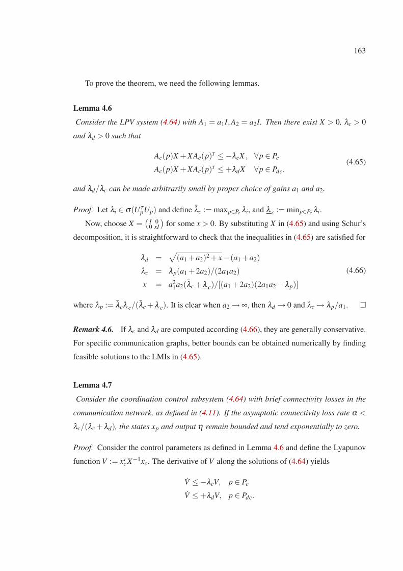
163

To prove the theorem, we need the following lemmas.

Lemma 4.6

Consider the LPV system (4.64) with A1 = a1I,A2 = a2I. Then there exist X > 0, λc > 0

and λd > 0 such that

Ac(p)X +XAc(p)T ≤−λcX , ∀p ∈ Pc

Ac(p)X +XAc(p)T ≤ +λdX ∀p ∈ Pdc.(4.65)

and λd/λc can be made arbitrarily small by proper choice of gains a1 and a2.

Proof. Let λi ∈ σ(UTpUp) and define λc := maxp∈Pc

λi, and λ c := minp∈Pcλi.

Now, choose X =(

I 00 xI

)

for some x > 0. By substituting X in (4.65) and using Schur’s

decomposition, it is straightforward to check that the inequalities in (4.65) are satisfied for

λd =√

(a1 +a2)2 + x− (a1 +a2)

λc = λp(a1 +2a2)/(2a1a2)

x = a21a2(λc +λ c)/[(a1 +2a2)(2a1a2 −λp)]

(4.66)

where λp := λcλ c/(λc +λ c). It is clear when a2 → ∞, then λd → 0 and λc → λp/a1.

Remark 4.6. If λc and λd are computed according (4.66), they are generally conservative.

For specific communication graphs, better bounds can be obtained numerically by finding

feasible solutions to the LMIs in (4.65).

Lemma 4.7

Consider the coordination control subsystem (4.64) with brief connectivity losses in the

communication network, as defined in (4.11). If the asymptotic connectivity loss rate α <

λc/(λc +λd), the states xp and output η remain bounded and tend exponentially to zero.

Proof. Consider the control parameters as defined in Lemma 4.6 and define the Lyapunov

function V := xTc X−1xc. The derivative of V along the solutions of (4.64) yields

V ≤−λcV, p ∈ Pc

V ≤ +λdV, p ∈ Pdc.

164

Then V ≤ [−λc(1− χ(p(t)))+λdχ(p(t))]V . By integrating the latter differential inequal-

ities, it is possible to show that

V (t) ≤V (τ)e−λc(t−τ−Tp(τ,t))+λdTp(τ,t), ∀t ≥ τ ≥ 0

which yields

V (t) ≤ e−[(1−α)λc−αλd ](t−t0)V (t0)e(1−α)(λc+λd)T0 , ∀t ≥ t0 ≥ 0

if the system has brief connectivity losses defined in (4.11). From the assumptions, λ :=

[(1−α)λc −αλd] > 0. Therefore, V (t) remains bounded and tends to zero, so does xc.

Moreover, by choosing r = min(x−1,a21/(λ 2

c + xa21)), then rCc(p)TCc(p) ≤ X−1, ∀p and

ηT(t)η(t) ≤ 1rV (t), thus completing the proof.

We are now ready to prove Theorem 4.9.

Proof of Theorem 4.9. Using (4.46) and Young’s inequality, it follows from (4.58) that

W ≤−λpW +g1‖η‖2 +g2‖δ‖2, (4.67)

for some λp,g1,g2 > 0, that is, the path-following subsystem with inputs η and δ and

state ζ is ISS. In Lemma 4.6, we have showed thatλd

λccan be made arbitrarily small by

increasing the gain a2. As a consequence α < 1/(1+ λd

λc) and therefore, from Lemma 4.7,

it follows that the CC subsystem is exponentially stable. Close examination of (4.67) and

(4.64) shows that the CC and PF subsystems form an interconnected cascade system. Since

the cascade interconnection of two ISS system is ISS, it follows that the resulting cascade

system with input δ and states ζ and xc is ISS.

Example 4.1. Consider the problem of coordinated CPF of a group of 3 vehicles, that

is, n = 3. Vehicle 2 is allowed to communicate with vehicles 1 and 3, but the latter two

do not communicate between themselves directly. We consider situation where there are

communication losses. Specifically, we assume that the failures in both links occur during

a maximum of 75% of the time, with the failures occurring periodically with a period of

10[sec], that is, α = 0.75 and T0 = 7.5[sec]. The corresponding eigenvalues defined in the

proof of Lemma 4.6 are given by λc = 3, λ c = 1 and λd = 2. For a1 = 1 and a2 = 1.6,

we have λc = 0.98 and λd = 0.12. Increasing a2 to 5 results in λc = 0.85 and λd = 0.01.

165

However, for a1 = 1 and a2 ≤ 1.5, there are no λc and λd that satisfy the conditions of

Lemma 4.6.

166

4.6 An illustrative example

This section illustrates the application of the previous results to underwater vehicles moving

in three-dimensional space.

Coordinated path-following of autonomous underwater vehicles (AUVs) in 3-D space

Consider an ellipsoidal shaped underactuated AUV not necessarily neutrally buoyant. Let

B be a body-fixed coordinate frame whose origin is located at the center of mass of the

vehicle and suppose that we have available a pure body-fixed control force τu in the xB

direction and two independent control torques τq and τr about the yB and zB axes of the

vehicle, respectively. The kinematics and dynamics equations of motion of the vehicle can

be written as (4.44) and (4.45), where

M = diagm11,m22,m33,J = diagJ11,J22,J33,u1 = τu,u2 = (τq,τr)

T ,B1 =(

100

)

,B2 =(

0 01 00 1

)

,

fν = −Dν(ν)ν − g1(R), fω = −Dω(ω)ω − g2(R)−S(ν)Mν −S(ω)Jω

Dν(ν) = diagXν1+X|ν1|ν1

|ν1|,Yν2+Y|ν2|ν2

|ν2|,Zν3

+Z|ν3|ν3|ν3|,

Dω(ω) = diagKω1+K|ω1|ω1

|ω1|,Mω2+M|ω2|ω2

|ω2|,Nω3

+N|ω3|ω3|ω3|,

g1(R) = RT

(

00

W−B

)

, g2(R) = S(rB)RT

(

00B

)

,

and gravitational and buoyant forces are given by W = mg and B = ρg∇, respectively,

where m is the mass of the vehicle, ρ is the mass density of the water, and ∇ is the volume

of displaced water. In the simulations presented here, the physical parameters match those

of the Sirene AUV described in (Aguiar & Pascoal 1997, Aguiar 2002).

Consider the CPF control of three underactuated AUVs. Vehicle 2 is allowed to com-

municate with vehicles 1 and 3, but the latter two do not communicate between themselves

directly. To simulate losses in the communications, we considered the situation where both

links fail 75% of the time, with the failures occurring periodically with a period of 10[sec].

Moreover, the information transmission delay is 5[sec]. Notice that during failures all the

links become deactivated. Since in this scenario, the valencies of the nodes vanish periodi-

cally, we apply the results of Lemma 4.5. In the simulations, we used the control law (4.42)

167

with ki = 0.1[sec−1] for i = 1,2,3.

Simulation results

In the simulations, the AUVs are required to follow paths of the form

pdi(γi) =

[

c1 cos(2πT

γi +φd),c1 sin(2πT

γi +φd),c2γi + z0i

]

,

with c1 = 20m, c2 = 0.05m, T = 400, φd = −3π4

, and z01= −10m,z02

= −5m,z03=

0m. The initial conditions are p1 = (5m,−10m,−5m), p2 = (5m,−15m,0m), p3 =

(5m,−20m,5m), R1 = R2 = R3 = I, and ν1 = ν2 = ν3 = ω1 = ω2 = ω3 = 0. The reference

speed vL was set to vL = 0.5[sec−1].

The vehicles are also required to keep a formation pattern that consists of having them

aligned along a common vertical line. Figure 4.2 shows the trajectories of the AUVs.

Figure 4.3 illustrates the evolution of the coordination and path-following errors while the

communication links fail periodically. Clearly, the vehicles adjust their speeds to meet

the formation requirements and the coordination errors γ12 := γ1 − γ2 and γ13 := γ1 − γ3

converge to zero.

4.7 Summary

This chapter addressed the problem of coordinated path-following control of a group vehi-

cles in the presence of varying communication topologies and fixed time-delays.

The key contributions of the chapter are twofold: i) the class of vehicle considered

is very general and encompasses underactuated vehicles, of which autonomous underwa-

ter vehicles with less number of actuators than degrees of freedom are an example, and

ii) problems that arise due to temporary communication losses and fixed time delay are

explicitly addressed in a rigorous mathematical framework.

A number of decentralized coordination schemes were developed. Two types of switch-

ing topologies were considered: brief connectivity losses and uniformly connected in mean.

Stability and convergence issues of the resulting coordinated path-following systems were

examined in detail. In the process, important properties of the interconnection of systems

with brief instabilities were derived.

168

−20−10

010

20

−20

−10

0

10

20

−10

0

10

20

30

y [m]

2D projection

x [m]

z [m

]

Figure 4.2: CPF of 3 AUVs with communication losses and time delays

169

0 50 100 150 200 250 300 350 4000

1

2

3

4

5

6

7

8

9

time [s]

[m]

||p1−p

d1||

||p2−p

d2||

||p3−p

d3||

(a) path-following errors

0 50 100 150 200 250 300 350 4000

2

4

6

8

10

12

14

time [s]

γ 1−γ 2

γ 1−γ 3

(b) Vehicle coordination errors

Figure 4.3: 75% of temporal communication losses; time delay 5[sec]

170

CHAPTER 5

CONCLUDING CHAPTER

This thesis addressed the problem of coordinated path-following (CFP) control of multiple

vehicles subjected to inter-vehicle communication constraints. The problem is well rooted

in challenging mission scenarios and has only recently come to the forum. Solutions were

proposed to the CFP problem and their efficacy assessed in simulation.

The strategies adopted have a solid theoretical foundation in Lyapunov-based and Graph

theory. The first is naturally suited for nonlinear system design and analysis, whereas the

latter is steadily becoming the tool par excellence to capture the topologies of different

communication scenarios. In this thesis it was shown how the two methodologies can be

brought together to yield tools that effectively allow a system designer to study the stability

and performance that can be obtained under different communication scenarios. To the best

of our knowledge, this work is the first contribution towards quantifying the performance

achievable with coordinated path-following control when the underlying communication

network is time-varying and exhibits fixed delays.

The results in this thesis lead naturally to algorithms for CPF control that are applicable

to heterogeneous fleets of vehicles evolving in 3D-space. The class of vehicle considered

is very general and encompasses underactuated vehicles, of which autonomous underwater

vehicles with less number of actuators than degrees of freedom are an example. Further-

more, the thesis addressed in a rigorous mathematical framework the problems that arise

due to temporary communication losses and fixed time delays. A number of decentralized

coordination schemes were developed and two types of switching topologies were consid-

ered: brief connectivity losses and uniformly connected in mean. Stability and convergence

171

172

issues of the resulting coordinated path-following systems were examined in detail. In the

process, important properties of the interconnection of systems with brief instabilities were

derived.

This work is a first step towards the derivation of advanced CPF algorithms for multiple

vehicles in the presence of communication constraints and time-delays. Few authors have

so far tackled these and related problems in a rigorous mathematical framework. Notable

exceptions are the results published in (Fossen 2002), (Skjetne et al. 2002), and in a re-

cent PhD thesis (Ihle 2006). See also (Arrichiello 2006) for a behavioral approach to the

coordinated control problem of multiple wheeled robots. This research path is largely un-

explored, and much work remains to be done towards the development of algorithms that

can withstand the transition from the laboratory to the real world. Especially challenging

is the development of new strategies to deal with the fact that communications occur asyn-

chronously at discrete instants of time, and that there are time-varying, distance-dependent

delays in the transmission of information among vehicles. Establishing a bridge between

the present work and the work that is being carried out in the field of networked control

systems is also important. A possible avenue of research is the inclusion of network ob-

servers as proposed in (Xu & Hespanha 2006) to facilitate the decision of when to transmit

information from one vehicle to its neighbors. The problem of coordinated navigation to

dispense with the use of expensive navigation systems installed on-board each vehicle war-

rants also further research effort. Finally, there is a need to prove the concepts developed

in actual trials with multiple vehicles on land, air, and at sea.

CHAPTER 6

APPENDIX

6.1 Path-following control implementation

To implement control laws (3.14), (3.15), (3.16), and (3.17), we need to have access to the

following values:

• Position and the orientation of the vehicle in U-frame, (x,y,ψB).

• The path defined in U-frame and associated with it a curvilinear abscissa s along

the path measured from some convenient reference point.

• Curvature cc(s) of the path as a function of s.

• Vehicle’s actual forward and angular velocities, (v,r).

• Estimation (using approximate derivative) of v. This can be done as well by substi-

tuting from the dynamics, knowing that v = F .

The procedure of calculation of control laws follows

1. Given s the variables ψT and p are known.

2. Compute (xe,ye) from (3.10).

3. Compute s from (3.15).

4. Compute xe, ye and ψe from (3.11).

173

174

5. Integrate s to compute s. The values of s used in step 1 come from this step.

6. Do the following computations in order

σ = −2ψa

π sign(v)arctanye

∂σ∂ye

= −2ψa

π sign(v) 11+y2

e

∂ 2σ∂y2

e= 2ψa

π sign(v) 2ye

(1+y2e)

2

7. σ = ∂σ∂ye

ye

8. s = vcosψe − vsinψeψe + k3xe

9. ye = −xeccs− xe∂cc

∂ ss2 − xeccs+ vsinψe + vcosψeψe

10. σ = ∂ 2σ∂y2

ey2

e + ∂σ∂ye

ye

11. φ = ccs+ σ − k1(ψe −σ)

12. and compute N from (3.14) or (3.16).

6.2 Proofs

Proof of Lemma 1.1

Proof. Partition the time interval [t0, t] along the sequence tk = t0 + kT for k = 0, ...,n so

that tn ≤ t < tn+1. Then tk+1 − tk = T . Integrating (1.7) over [tk, tk+1] yields

x(tk+1) = e−a∫ tk+1

tk(1−p(t))dt

x(tk).

Therefore,

|x(tk+1)| ≤ e−a(1−α)T |x(tk)| ⇒ |x(tn)| ≤ e−na(1−α)T |x(t0)|.

Integrating (1.7) over [tn, t], we have |x(t)| ≤ |x(tn)| where we used the fact that 1− p(t)≥ 0.

By combining the above inequalities and using the fact that t − t0 ≤ (n+1)T , we get

|x(t)| ≤ be−β (t−t0)|x(t0)|

where b = ea(1−α)T and β = (1−α)a and the result follows.

175

Proof of Lemma 4.1

1. Since Rank(I −Lβ ) = 1, Lβ has n−1 eigenvalue at 1. Using the definition of Lβ ,

it can be easily verified that Lβ 1 = 0 and β TLβ = 0T , that is zero is an eigenvalue.

Therefore, we can conclude that zero is a single eigenvalue.

2. Lβ KLp = (K − 1β T 1

11T)Lp = KLp, since 1T Lp = 0T .

3. Following some computations we get L T

β K−1Lβ = K−1 − 1β T 1

ββ T . Then

νTL T

β K−1Lβ ν = νT K−1ν − 1β T 1

νT ββ T ν ≤ νT K−1ν for any ν ∈ Rn and equality

happens for β T ν = 0, thus the result follows.

4. The result follows from the facts that γ = Lβ γ , Lβ 1 = 0 and RankLβ = n−1.

5. Follows from the definition of γ in (4.12).

6. Follows from the definition of γ and the fact that Lp1 = 0.

7. Notice that

|γi − γ j|2 = γ2i + γ2

j −2γiγ j ≤ 2(γ2i + γ2

j ) ≤ 2‖γ‖2 < 2ε2.

but γi− γ j = γi−γ j, thus |γi−γ j|<√

2ε . For the next part, notice that KLpγ = KLpγ ,

then ‖KLpγ‖ ≤ ‖K‖.‖Lp‖.‖γ‖ ≤ nε‖K‖, where we used the fact that ‖Lp‖ ≤ n and

equality happens for a complete graph, that is, p = [1, ...,1]T .

8. Recall the fact that if the graph is connected (p ∈ Pc), then Lp has a single eigenvalue

at zero associated to the (right and left) eigenvector 1, and the rest of the eigenvalues

are positive. Let L be a representative graph Laplacian of Lp for p ∈ Pc. Then,

there is a unitary matric U = [u1, ...,un] where u1 = 1√n1 and a diagonal matrix Λ =

diag[λ1,λ2, ...,λn] with 0 = λ1 < λ2 ≤ ... ≤ λn, such that L = UΛUT . Then for any

ν ∈Rn, we have

νT Lν = ∑ni=1 λi(u

Ti ν)2

= ∑ni=2 λi(u

Ti ν)2

≥ λ2 ∑ni=2(u

Ti ν)2

= λ2 ∑ni=1(u

Ti ν)2 −λ2(u

T

1ν)2

= λ2νT ν −λ21n(1T ν)2.

176

To compute λ2,m, simply observe that the second term is zero, therefore λ2,m is the

minimum λ2 over p ∈ Pc. Now if β 6= 1, an standard minimization of vector function

νT ν − 1n(1T ν)2 with constraints β T ν = 0 and νT ν = 1, yields the results. Similarly,

it can be shown that λm > 0. Numerical computations show that λ2,m = λm.

9. Recall that the graph Laplacian is L = D−A. Using the definitions of degree matrix

D and adjacency matrix A, by inspection, it is easy to show the result.

Proof of (4.27)

Denote the i’th column (or row) of Lp by li,p. Then vri= kil

Ti,pγ . Now

∑i |vri|2 = ∑i k2

i γT li,plTi,pγ

= γT ∑i k2i li,plT

i,pγ

= γT LpK2Lpγ

= γT LpK2Lpγ.

Therefore since maxp,‖ν‖=1 νT Lpν = n, the result follows. Notice that in this optimization,

the equality happens for a complete graph, and n is the largest eigenvalue for all combina-

tions of p.

Proof of Proposition 4.3 (system interconnection)

Choose V =V1 +aV2 for some a > 0 which is to be chosen later. Clearly, V satisfies the first

condition of (4.20) for some α > 0, α > 0. Next, we will show that the second condition is

also satisfied. Taking derivative of V yields

V ≤−(λ1 −ag2

α1

)V1 −a(λ2 −g1

aα2

)V2 +g‖d‖2

where g = max(1,a). At this stage assume g1 and g2 are nonzero. Let

λ0 = λ1 −ag2

α1

= λ2 −g1

aα2

. (6.1)

177

• λ2(t) = λ2 > 0: If there exist positive numbers λ0 and a satisfying (6.1), then V ≤−λ0V +

g‖d‖2 and therefore the interconnected system is ISS from d. The condition of existence

of positive solutions is g1g2 < α1α2λ1λ2. From there the convergence rate is λ = λ0.

• λ2(t) has brief instabilities: Using the same Lyapunov function V = V1 + aV2 and λ0 as

in (6.1), compute the derivative of V to obtian

V ≤−λ0V +a(λ2 −λ2(t))V2 +g‖d‖2

which yields

V ≤

−λ0V +g‖d‖2 χ(p) = 0

(λ3 −λ0)V +g‖d‖2 χ(p) = 1,

where λ3 := λ2 + λ2. Again such λ0 exists if g1g2 < α1α2λ1λ2. Integrating the above

differential inequalities and following similar computations as in (Hespanha et al. 2004), it

is easy to show that

V (t) ≤ V (t0)e−λ0(t−t0−Tp)+λ4Tp+

gsup[t0,t]‖d‖2

∫ tt0

e−λ0(t−τ−Tp)+λ4Tpdτ

where λ4 := λ3 −λ0. Notice that λ4 ≥ 0. This yields

V (t) ≤V (t0)e−(λ0−αλ3)(t−t0)+λ3Tα +

eλ3Tα

λ0 −αλ3gsup[t0,t]

d2

where Tα = (1−α)T0, if the system has brief instabilities defined in (4.11). Therefore, the

interconnected system is ISS from d as input if α < λ0/λ3.

If g2 = 0 and g1 > 0, the interconnected system takes a cascade configuration and the

dynamics of system 2 are reduced to

V2 ≤

−λ2V2 +d22 χ(p) = 0

λ2V2 +d22 χ(p) = 1,

whose solution takes the form

V2(t) ≤V2(t0)e−(λ2−αλ3)(t−t0)+λ3Tα +

eλ3Tα

λ2 −αλ3sup[t0,t]

d22

where λ3 = λ2 + λ2. Substituting it in the dynamics of system 1 and integration yields

V1(t) ≤ a1e−λ1t +a2e−(λ2−αλ3)t +a3sup[t0,t]‖d‖2.

for some ai ∈R. Therefore, the cascade system is ISS from d as input if α < λ2/(λ2 + λ2)

and the convergence rate will be min(λ1,(1−α)λ2 −αλ2).

178

Proof of Lemma 4.2

Proof. We first show that MMT Mp = Mp. Since MT M = I, then MMT has n−1 eigenvalues

at 1 and one eigenvalue at 0. Thus, Rank(I − MMT ) = 1 and using the fact that (I −MMT )1 = 1, then (I − MMT )ν = 0 if ν ∈ 1⊥ (the orthogonal space). On the other hand,

MTp1 = 0, that is, Mp has n−1 columns orthogonal to 1. Therefore (I − MMT )Mp = 0, or

MMT Mp = Mp. Thus MTp = MT

pMMT = UpMT . To prove the second part of the Lemma,

notice that

σ(U TpUp) = σ(UpU T

p ) = σ(MTpMMT Mp)

= σ(MTpMp) = σ(MpMT

p)\0.

Lemma 6.1

Lemma 6.1

Let G be a connected (undirected) graph with Laplacian L of dimension n× n and let

C(t) = diag[cii]n×n be a diagonal matrix satisfying c1I ≤C(t) ≤ c2I; c1 > 0. Define

Q(t) = C−1(t)A−1L+LC−1(t)A−1 +2C(t)−1A,

where A = diag[aii]n×n > 0 and a1I ≤ A ≤ a2I. Suppose

a21 >

1

2(c2

c1− a1

a2)max

idi (6.2)

where di = |Ni| is the cardinality of Ni, that is, the index set of the neighbors of vertex i in

Graph G . Then, there exists γ > 0 such that ‖Q(t)‖ > γ for all t ≥ 0.

Proof. L has the property that all its diagonal elements are positive and the off diagonals

are non-positive. Because A and C are diagonal, Q inherits that property. This, together

with Gersgorin’s theorem (Horn & Johnson 1985) imply that if

n

∑j=1

qi j(t) > γ, ∀i (6.3)

for some γ > 0, then λmin(Q(t)) > γ for all t, equivalently Q1 > γ1, where the inequality

should be interpreted element by element. Because L1 = 0, the above condition degenerates

179

to

L

[

1

ciiaii

]

n×1

+

[

2aii

cii

]

n×1

> γ1

or 2aii

cii+ ∑ j∈Ni

( 1ciiaii

− 1c j ja j j

) > γ for all i, where we used the properties of L. There-

fore, (6.3) is satisfied if

2a1

c2+di(

1

a2c2− 1

a1c1) > γ, ∀i

which is equivalent to (6.2) because γ can be taken arbitrarily small.

A proof for Proposition 3.1 under assumption i

Since v(t) is uniformly continuous and limt→∞ v(t) 6= 0, we have

∃ε1,ε2 > 0,∃T = T (ε1) > 0,τ−n ,τ+n ;n ≥ 1, such that

τ+n − τ−n ≥ ε2, τ−n+1 > τ+

n , τ−1 > T

and ∀t ∈ [τ−n ,τ+n ), |v(t)| > ε1. That is, after some time T , v(t) is larger than some ε1 > 0

over an infinite number of finite intervals. Therefore, using (3.20), it is easily seen that for

all t ∈ [τ−n ,τ+n ) and some λ > 0, Vp ≤−λVp whose integration yields

Vp(τ+n ) ≤Vp(τ

−n )e−λε2. (6.4)

Since τ−n+1 > τ+n , V ≤ 0 implies that Vp(τ

−n+1)≤Vp(τ

+n ) and using (6.4) we get Vp(τ

−n )≤

Vp(τ−0 )e−nλε2 , thus showing that limn→∞Vp(τ

−n ) = 0. That is Vp(t) is a nondecreasing func-

tion that tends to zero. This in turn implies that Xp converges asymptotically to 0. Thus

Xp = 0 is semi-globally asymptotically stable.

180

BIBLIOGRAPHY

Aguiar, A. P. (2002), Nonlinear Motion Control of Nonholonomic and Underactuated Sys-

tems, PhD thesis, Dept. Electrical Engineering, Instituto Superior Tecnico, IST, Lisbon,

Portugal. 92, 166

Aguiar, A. P., Ghabcheloo, R., Pascoal, A., Silvestre, C., Hespanha, J. & Kaminer, I.

(2006), Coordinated path-following of multiple underactuated autonomous vehicles with

bi-directional communication constraints, in ‘International Symposium on Communica-

tion, Control and Signal Processing (ISCCSP)’, Morocco. 26, 27, 28

Aguiar, A. P. & Hespanha, J. P. (2004), Logic-based switching control for trajectory-

tracking and path-following of underactuated autonomous vehicles with parametric mod-

eling uncertainty, in ‘Proc. of the 2004 Amer. Contr. Conf.’, Boston, MA, USA. 156

Aguiar, A. P. & Hespanha, J. P. (2006), ‘Trajectory-tracking and path-following of under-

actuated autonomous vehicles with parametric modeling uncertainty’, IEEE Trans. on

Automat. Contr. In press. 132, 156, 158

Aguiar, A. P., Hespanha, J. P. & Kokotovic, P. (2005), ‘Path-following for non-minimum

phase systems removes performance limitations’, IEEE Transactions on Automatic Con-

trol 50(2), 234–239. 132

Aguiar, A. P. & Pascoal, A. M. (1997), Modeling and control of an autonomous underwa-

ter shuttle for the transport of benthic laboratories, in ‘Proc. of the Oceans’97 Conf.’,

Halifax, Nova Scotia, Canada. 166

Arrichiello, F. (2006), Coordination Control of Multiple Mobile Robots, Phd thesis, Uni-

versita Degli Studi di Cassino, Cassino, Italy. 172

Balakrishnan, R. & Ranganathan, K. (2000), A Textbook of Graph Theory, Springer. 73, 76

181

182

Bang-Jensen, J. & Gutin, G. (2002), Digraph theory, algorithms and applications, Springer.

73

Beard, R., Lawton, J. & Hadaegh, F. (2001), ‘A coordination architecture for spacecraft

formation control’, IEEE Trans. on Contr. Systems Tech. 9, 777–790. 16

Bertsekas, D. & Tsitsiklis, J. (1989), Parallel and Distributed Computation: Numerical

Methods, Prentice Hall. 23

Biggs, N. (1996), Algebraic graph theory, Second Edition. Cambridge University Press.

73, 75

Blondel, V. D., Hendrickx, J. M., Olshevsky, A. & Tsitsiklis, J. N. (2005), Convergence in

multiagent coordination, consensus, and flocking, in ‘Proc. of the 44th IEEE CDC-ECC’,

Seville, Spain. 23

Børhaug, E., Pavlov, A., Ghabcheloo, R., Pettersen, K., Pascoal, A. & Silvestre, C. (2006),

Formation control of underactuated marine vehicles with communication constraints,

in ‘Proc. of the 7th IFAC Conference on Maneuvering and Control of Marine Craft

(MCMC’06)’, Lisbon, Portugal. 28

Bullo, F. & Cortes, J. (2005), Adaptive and distributed coordination algorithms for mobile

sensing networks, in V. Kumar, N. E. Leonard & A. S. Morse, eds, ‘Cooperative Control.

(Proceedings of the 2003 Block Island Workshop on Cooperative Control)’, Vol. 309 of

Lecture Notes in Control and Information Sciences, Springer Verlag, New York, pp. 43–

62. 16

Cao, M., Morse, A. S. & Anderson, B. D. O. (2006a), ‘Agreeing asynchronously in contin-

uous time’, IEEE Transactions on Automatic Control, submitted . 23

Cao, M., Morse, A. S. & Anderson, B. D. O. (2006b), ‘Reaching a consensus in a dynam-

ically changing environment delays and asynchronous events’, SIAM J. on Control and

Optimization, submitted . 23

Caughman, J., Lafferriere, G., Veerman, J. J. P. & Williams, A. (2005), ‘Decentralized

control of vehicle formation’, Systems and Control Letters . 21, 22, 79

183

Cortes, J. & Bullo, F. (2005), ‘Coordination and geometric optimization via distributed

dynamical systems’, SIAM Journal on Control and Optimization 44(5), 1543–1574. 16

Dobrokhodov, V., Kaminer, I., Jones, K. & Ghabcheloo, R. (2006), Vision-based track-

ing and position estimation for moving targets using small UAVs, in ‘American Control

Conference (ACC)’, Minneapolis, Minnesota, USA. 28

Egerstedt, M. & Hu, X. (2001), ‘Formation constrained multi-agent control’, IEEE Trans.

on Robotics and Automation 17(6), 947 – 951. 16, 18

Encarnacao, P. & Pascoal, A. (2001), Combined trajectory tracking and path following: an

application to the coordinated control of marine craft, in ‘Proc. of IEEE Conf. Decision

and Control (CDC)’, Orlando, Florida. 16, 17

Fang, L., Antsaklis, P. J. & Tzimas, A. (2005), Asynchronous consensus protocols: pre-

liminary results, simulations and open questions, in ‘Proc. of the 44th IEEE CDC-ECC’,

Seville, Spain, pp. 2194–2199. 16

Fax, A. & Murray, R. (2002a), Graph Laplacians and stabilization of vehicle formations,

in ‘Proc. of IFAC World Congress’, Barcelona, Spain. 3, 19, 22

Fax, A. & Murray, R. (2002b), Information flow and cooperative control of vehicle forma-

tions, in ‘Proc. of IFAC World Congress’, Barcelona, Spain. 3, 19

Fax, J. A. (2002), Optimal and Cooperative Control of Vehicle Formations, Phd thesis,

California Institute of Technology, Pasadena, California, USA. 73

Fiedler, M. (1973), ‘Algebraic connectivity of graphs’, Czechoslavak Mathematical Jour-

nal 23(98), 298–306. 20

Fossen, T. (1994), Guidance and Control of Ocean Vehicles, John Willey & Sons, Inc.,

New York. 156

Fossen, T. (2002), Marine Control Systems: Guidance, Navigation and Control of Ships,

Rigs and Underwater Vehicles, Marine Cybernetics AS, ISBN 82-92356-00-2. 2, 17,

172

184

Ghabcheloo, R., Aguiar, A. P., Pascoal, A., Silvestre, C., Hespanha, J. & Kaminer, I.

(2006), ‘Coordinated path-following control of multiple vehicles in the presence of com-

munication losses and time delays’, Submitted to SIAM, special issue on Control and

Optimization in Cooperative Networks . 24, 27

Ghabcheloo, R., Aguiar, A., Pascoal, A. & Silvestre, C. (2006), Coordinated path-following

control of multiple AUVs in the presence of communication failures and time delays,

in ‘Proc. of the 7th IFAC Conference on Maneuvering and Control of Marine Craft

(MCMC’06)’, Lisbon, Portugal. 26, 27

Ghabcheloo, R., Aguiar, A., Pascoal, A., Silvestre, C., Kaminer, I. & Hespanha, J. (2006),

Coordinated path-following control of multiple underactuated autonomous vehicles in

the presence of communication failures, in ‘Proc. of the 45th IEEE Conference on Deci-

sion and Control (CDC’06)’, San Diego, California USA. 18, 24, 26, 27

Ghabcheloo, R., Carvalho, D., Pascoal, A. & Silvestre, C. (2005), Coordinated motion

control of multiple autonomous underwater vehicles, in ‘Proc. of International Workshop

on Underwater Robotics (IWUR)’, Genoa, Italy. 26

Ghabcheloo, R., Pascoal, A. & Silvestre, C. (2004), Coordinated path-following

control using linearization techniques, Internal Report CPF01L, Instituto Superior

Tecnico/Institute for Systems and Robotics. 24

Ghabcheloo, R., Pascoal, A. & Silvestre, C. (2005a), Coordinated path-following

control using nonlinear techniques, Internal Report CPF02NL, Instituto Superior

Tecnico/Institute for Systems and Robotics. 24, 25

Ghabcheloo, R., Pascoal, A. & Silvestre, C. (2005b), Nonlinear coordinated path-following

control of multiple wheeled robots with communication constraints, in ‘Proc. of Interna-

tional Conference on Advanced Robotics (ICAR)’, Seattle, USA. 17, 26

Ghabcheloo, R., Pascoal, A., Silvestre, C. & Kaminer, I. (2004), Coordinated path-

following control of multiple wheeled robots, in ‘Proc. of the 5th IFAC Symposium

on Intelligent Autonomous Vehicles’, Lisbon, Portugal. 24, 25

185

Ghabcheloo, R., Pascoal, A., Silvestre, C. & Kaminer, I. (2005), Coordinated path follow-

ing control of multiple wheeled robots with directed communication links, in ‘Proc. of

the 44th IEEE Conference on Decision and Control and European Control Conference

(CDC-ECC)’, Seville, Spain. 26

Ghabcheloo, R., Pascoal, A., Silvestre, C. & Kaminer, I. (2006a), ‘Coordinated path-

following control of multiple wheeled robots using linearization techniques’, Interna-

tional Journal of Systems Science 37(6), 399–414. 24, 25

Ghabcheloo, R., Pascoal, A., Silvestre, C. & Kaminer, I. (2006b), Group Coordination and

Cooperative Control, Vol. 336 of ISBN: 3-540-33468-8, Springer-Verlag, chapter Coor-

dinated Path-Following Control of Multiple Vehicles subject to Bi-directional Commu-

nication Constraints, pp. 93–111. 24, 25, 26

Ghabcheloo, R., Pascoal, A., Silvestre, C. & Kaminer, I. (2007), ‘Nonlinear coordinated

path-following control of multiple wheeled robots with bi-directional communication

constraints’, International Journal of Adaptive control and signal Processing 21(2-

3), 133 – 157. 16, 24, 25, 26, 132

Giuletti, F., Pollini, L. & Innocenti, M. (2000), ‘Autonomous formation flight’, IEEE Con-

trol Systems Magazine 20, 33–34. 16

Godsil, C. & Royle, G. (2001), Algebraic Graph Theory, Graduated Texts in Mathematics,

Springer-Verlag New York, Inc. 73, 74, 135

Hespanha, J. M., Yakimenko, O. A., Kaminer, I. I. & Pascoal, A. M. (2004), ‘Linear para-

metrically varying systems with brief instabilities: An application to vision/inertial nav-

igation’, IEEE Trans. on Aerospace and Electronics Systems 40(3), 889–900. 136, 141,

149, 177

Horn, R. A. & Johnson, C. R. (1985), Matrix Analysis, Cambridge Univ. Press. 66, 73, 178

Ihle, I.-A. F. (2006), Coordinated Control of Marine Craft, Phd thesis, Norwegian Univer-

sity of Science and Technology, Trondheim, Norway. 18, 172

186

Ito, H. (2002), A constructive proof of ISS small-gain theorem usign generalized scaling,

in ‘Proc. of IEEE Conference on Decision and Control’. 143

Jadbabaie, A., Lin, J. & Morse, A. (2003), ‘Coordination of groups of mobile autonomous

agents using nearest neighbor rules’, IEEE Trans. on Automatic Control 48(6). 16, 22,

144

Kaminer, I., Pascoal, A., Hallberg, E. & Silvestre, C. (1998), ‘Trajectory tracking for au-

tonomous vehicles: An integrated approach to guidance and control’, Journal Of Guid-

ance, Control, and Dynamics 21(1), 29–38. 35

Kaminer, I., Pascoal, A., Khargonekar, P. & Coleman, E. (1995), ‘A velocity algorithm for

the implementation of gain-scheduled controllers’, Automatica 31(1), 1185–1191. 37,

38, 45, 47, 48

Kaminer, I., Pascoal, A. & Yakimenko, O. (2005), Nonlinear path following control of fully

actuated marine vehicles with parameter uncertainty, in ‘Proc. of the 16th IFAC World

Congress’, Prague, Czech Republic. 87

Khalil, H. K. (2002), Nonlinear Systems, Third Edition, Prentice Hall. 37, 66, 69, 88, 120,

133

Kim, Y. & Mesbahi, M. (2006), ‘On maximizing the second smallest eigenvalue of state-

dependent graph Laplacian’, IEEE Trans. on Automatic Control 51(1), 116–120. 16

Kyrkjebo, E. (2007), Motion Coordination of Mechanical Systems: Leader-Follower Syn-

chronization of Euler-Lagrange Systems Using Output Feedback Control, PhD thesis,

the Norwegian University of Science and Technology, Trondheim, Norway. 3

Kyrkjebo, E. & Pettersen, K. (2003), Ship replenishment using synchronization control,

in ‘Proc. of the 6th IFAC Conference on Manoeuvering and Control of Marine Craft

(MCMC)’, Girona, Spain. 17

Kyrkjebo, E., Wondergen, M., Pettersen, K. & Nijmeijer, H. (2004), Experimental results

on synchronization control of ship rendezvous operations, in ‘Proc. of the 6th IFAC

Conference on Control Applications in Marine Systems’, Ancona,Italy. 17

187

Lapierre, L., Soentanto, D. & Pascoal, A. (2003), Coordinated motion control of marine

robots, in ‘Proc. of the 6th IFAC Conference on Manoeuvering and Control of Marine

Craft (MCMC)’, Girona, Spain. 16, 17

Lin, J., Morse, A. S. & Anderson, B. D. O. (2004), ‘The multi-agent rendezvous problem -

part 2: The asynchronous case’, SIAM J. on Control and Optimization, submitted . 23

Lin, J., Morse, A. S. & Anderson, B. D. O. (2006), ‘The multi-agent rendezvous problem -

part 1: The synchronous case’, SIAM J. on Control and Optimization, to appear . 23

Lin, Z. (2006), Coupled Dynamic Systems: From Structure Towards Stability And Stabi-

lizability, Phd thesis, University of Toronto, Toronto, Canada. 73, 79, 139, 141

Lin, Z., Francis, B. & Maggiore, M. (2005a), ‘Necessary and sufficient graphical condi-

tions for formation control of unicycles’, IEEE Trans. on Automatic Control 50(1), 121–

127. 20, 21, 22, 79

Lin, Z., Francis, B. & Maggiore, M. (2005b), ‘State agreement for coupled nonlinear sys-

tems with time-varying interaction’, under revision: SIAM Journal on Control and Op-

timization . 16, 139, 140, 141

Massera, J. L. (1949), ‘On Liapounoff’s conditions of stability’, Annals of Mathematics

50(3), 705–721. 71

Mesbahi, M. (2002), On a dynamic extension of the theory of graphs, in ‘Proc. of the

American Control Conference’, Anchorange, AL, USA. 20

Mesbahi, M. & Hadaegh, F. (2001), ‘Formation flying control of multiple spacecraft via

graphs, matrix inequalities, and switching’, Journal of Guidance, Control and Dynamics

24(2), 369–377. 20

Micaelli, A. & Samson, C. (1993), Trajectory-tracking for unicycle-type and two-steering-

wheels mobile robots, Technical Report 2097, INRIA, Sophia-Antipolis, France. 34, 36,

82, 83

188

Moreau, L. (2004), Stability of continuous-time distributed consensus algorithm, in ‘Proc.

of the 43rd IEEE Conference on Decision and Control’, Atlantis, Paradise Island, Ba-

hamas, pp. 3998 – 4003. 139, 140, 141

Moreau, L. (2005), ‘Stability of multiagent systems with time - dependent communication

links’, IEEE Trans. on Automatic Control 50(2). 22, 23

Ogren, P., Egerstedt, M. & Hu, X. (2002), ‘A control Lyapunov function approach to mul-

tiagent coordination’, IEEE Trans. on Robotics and Automation 18, 847 – 851. 16

Olfati Saber, R. & Murray, R. (2003a), Agreement problems in networks with directed

graphs and switching topology, in ‘Proc. of Conference on Decision and Control (CDC)’,

Hawaii, USA. 20, 22

Olfati Saber, R. & Murray, R. M. (2003b), Consensus protocols for networks of dynamic

agents, in ‘American Control Conference’, Denver, CO, USA. 20

Papachritodoulou, A. & Jadbabaie, A. (2005), Synchronization in oscilator networks:

Switching topologies and non-homogenous delays, in ‘Proc. of the 44th IEEE Confer-

ence on Decision and Control(CDC)’, Seville, Spain. 16

Pascoal, A., Silvestre, C. & Oliveira, P. (2006), ‘Vehicle and mission control of single and

multiple autonomous marine robots’, IEE Control Engineering Series, G. Roberts and

R. Sutton (Eds) pp. 353–386. 2, 17

Pascoal et al., A. (2000), Robotic ocean vehicles for marine science applications: the eu-

ropean ASIMOV project, in ‘Proc. of OCEANS MTS/IEEE’, Rhode Island, Providence,

USA. 1

Pratcher, M., D’Azzo, J. & Proud, A. (2001), ‘Tight formation control’, Journal of Guid-

ance, Control and Dynamics 24(2), 246–254. 16

Rouche, N., Habets, P. & Laloy, M. (1977), Stability theory by Liapunov’s direct method,

Springer-Verlag New York, Inc. 66, 68, 71

189

Sepulchre, R., Paley, D. & Leonard, N. (2003), Collective motion and oscillator synchro-

nization, in ‘Proc. of Block Island Workshop on Cooperative Control’. 16

Silvestre, C. & Pascoal, A. (2002), ‘On the design of gain-scheduled trajectory tracking

controllers’, International Journal of Robust and Nonlinear Control 12, 797–839. 33, 35

Sivestre, C. (2000), Multi-Objective Optimization Theory with Applications to the Inte-

grated Design of Controllers Plants for Autonomous Vehicles, Phd thesis (in english),

Instituto Superior Tecnico, Lisbon, Portugal. 33, 35, 37

Skjetne, R., Flakstad, I. & Fossen, T. (2003), Formation control by synchronizing multi-

ple maneuvering systems, in ‘Proc. of the 6th IFAC Conference on Manoeuvering and

Control of Marine Craft (MCMC)’, Girona, Spain. 17

Skjetne, R., Fossen, T. I. & Kokotovic, P. K. (2004), ‘Robust output maneuvering for a

class of nonlinear systems’, Automatica 40(3), 373–383. 132

Skjetne, R., Moi, S. & Fossen, T. I. (2002), Nonlinear formation control of marine craft, in

‘Proc. of the 41st Conf. on Decision and Contr.’, Las Vegas, NV. 16, 17, 172

Soetanto, D., Lapierre, L. & Pascoal, A. (2003), Adaptive, non-singular path following,

control of dynamic wheeled robots, in ‘Proc. of ICAR’, Coimbra, Portugal. 82, 87

Sontag, E. D. (1998), Mathematical control theory, deterministic finite dimensional sys-

tems, Texts in Applied Mathematics 6, Second Edition, Springer-Verlag New York, Inc.

133

Sontag, E. D. & Wang, Y. (1996), ‘New characterizations of input-to-state stability’, IEEE

Trans. on Automatic Control 41(9), 1283–1294. 69, 133

Tanner, H., Jadbabaie, A. & Pappas, G. (2004), ‘Flocking agents with varying interconnec-

tion topology’, submitted to Automatica . 23

Tsitsiklis, J. N. & Athans, M. (1984), ‘Convergence and asymptotic agreement in dis-

tributed decision problems’, IEEE Transaction on Automatic Control . 16, 23, 144

190

Vicsek, T., Czirok, A., Ben Jacob, E., Cohen, I. & Schochet, O. (1995), ‘Novel type of

phase transitions in a system of self-driven particles’, Phys. Rev. lett. 75, 1226–1229. 22

Xu, Y. & Hespanha, J. (2006), Communication logic design and analysis for networked

control systems, Current trends in nonlinear systems and control, Boston: Birkhauser.

172

Yakimenko, O., Kaminer, I., Pascoal, A. & Ghabcheloo, R. (2006), Path generation, path

following and coordinated control for time-critical missions of multiple UAVs, in ‘Amer-

ican Control Conference (ACC)’, Minneapolis, Minnesota, USA. 28

Zhou, K., Doyle, J. & Glover, K. (1996), Robust and Optimal Control, Prentice Hall. 40