by N MT. Reddy

NASA CONTRACTOR

REPORT

- 011 OZ IT= 011 O- 0-m .I=-

-

CR-78 E -- .--__

THE USE OF SELF-CALIBRATING CATALYTIC PROBES TO MEASURE FREE-STREAM ATOM CONCENTRATION IN A HYPERSONIC FLOW

by N MT. Reddy

Prepared by

UNIVERSITY OF TORONTO

Toronto, Canada

f Or

*

’ NATIONAL AERONAUTICS AND SPACE ADMINISTRATION . WASHINGTON, D. C. l MAY 1967 /

f

TECH LIBRARY KAFB, NM

llClb0Clb4 NASA CR-760

THE USE OF SELF-CALIBRATING CATALYTIC PROBES TO MEASURE

FREE-STREAM ATOM CONCENTRATION IN A HYPERSONIC FLOW

By N. M. Reddy

Distribution of this report is provided in the interest of information exchange. Responsibility for the contents resides in the author or organization that prepared it.

Prepared under Grant No. NsG-633 by UNIVERSITY OF TORONTO

Toronto 5, Canada

for

NATIONAL AERONAUTICS AND SPACE ADMINISTRATION

For sale by the Clearinghouse for Federal Scientific and Technical Information

Springfield, Virginia 22151 - CFSTI price $3.00

ACKNOWLEDGEMENTS

I am very much indebted to Dr. G. N. Patterson for the oppor- tunity to carry out this research at the Institute for Aerospace Studies;

This work was supervised by Dr. I. I. Glass. I particularly appreciate the stimulating guidance and suggestions that I received from him during the course of this work. I wish to thank Dr. P. A. Sullivan for a critical reading of my thesis.

I am indebted to the Canadian Commonwealth Scholarship Committee for providing me with financial assistance over a period of two years.

The financial assistance received from NASA under Grant NsG-633 and the Canadian National Research Council and Defence Research Board is gratefully acknowledged,

iii

SUMMARY

A technique is presented to measure simultaneously the catalytic efficiency (@Q and the free stream atom concentration (CT& in a hypersonic flow of dissociated gas. The principle involved is to measure the differential heat transfers by using, either a combination of axisymmetric and two-dimensional, differential catalytic probes, or two geometrically similar, differential catalytic probes mounted side by side in a uniform, dissociated, hypersonic free-stream. Using these measured quantities in the appropriate stagnation point heat transfer relations for a frozen flow, simple formulae for #c and a,, are derived. The feature of these formulae is that,unlike the full expression for stagnation point heat transfer, they are independent of such quantities as viscosity, velocity, and density. Only the stagnation enthalpy and the Lewis number, need to be known. This self-calibrating principle is shown to apply not only in the boundary layer regime but also in the viscous shock layer (merged layer) regime. The most suitable geometric proportions for the gauges are given.

The practical feasibility of this technique has been successfully demonstrated by measuring the gauge catalytic efficiency of a silver surface and the free-stream oxygen atom concentrations in the UTIAS 11 in. x 15 in. Hypersonic Shock Tunnel test section. The free-stream atom concentration cyo-, was measured at five reservoir conditions (14.2 atmos. -L PO C 40.7 atmos., 4530°K G To d 4700°K., 0. 54 2 CYST/ 0. 32) and varied from 0. 30 to 0. 16. Dur- ing these measurements the probe Reynolds numbers (Rep), based on flow conditions behind the bow shock, varied from 59 to 122 for the axisymmetric probe and 98 to 202 for the two-dimensional probe. The test section Mach number (Ma-J varied from 15 to 17. The measured values of (Ye compared favourably with those computed from coupled vibrational and dissociational nonequilibrium nozzle flow calculations carried out by Tirumalesa (Ref. 14).

I

TABLE OF CONTENTS

Page

NOTATION ix

INTRODUCTION 1

1. A BRIEF REVIEW OF THE THEORY OF CATALYTIC 4 PROBES TO MEASURE ATOM CONCENTRATIONS

2. THEORETICAL CONSIDERATIONS OF A SELF-CALIBRATING ‘7 PROBE

2. 1 Introduction and Assumptions 7 2. 2 Boundary Layer Regime 9

2. 2. 1 Combination of Axisymmetric and Two- Dimensional Probes 9

2. 2. 2 Combination of Geometrically Similar Probes 11

2. 3 Merged Layer Regime 12

3. EXPERIMENTAL FACILITY AND ITS CALIBRATION 17

3. 1 Shock Tube, Nozzle System and Test Section 17 3. 2 Reservoir Conditions 19 3. 3 Nonequilibrium Nozzle Flow Calculations 22 3. 4 Test Section Flow Calibration 23

4. DESIGN CONSIDERATIONS OF CATALYTIC PROBES 24

4. 1 Introductory Remarks 24 4. 2 Frozen Boundary Layer and Frozen Shock Layer Criteria 25

4. 2.1 Frozen Boundary layer 25 4.2. 2 Frozen Shock-Layer 25

4. 3 Selection of Probe Sizes and Configurations 27

5. EXPERIMENTS AND RESULTS 28

5.1 Introductory Remarks 28 5.2 Coating Technique of Heat Transfer Gauges 29 5.3 Arrangement of Catalytic Probes 30 5.4 Effect of Radiation on Measured Heat Transfers 31 5.5 Experimental Procedure 31 5. 6 Reduction of Data 33 5. 7 Estimation of qc and ao, 33

vii

-- ...__ ..-.._-. --..-. .., ,. ,, , . . , ,. , . . ..I .I.-m-..-m . I I I I . ..-a .,,, II

6. DISCUSSION OF RESULTS AND CONCLUSIONS

REFERENCES

34

39

TABLES

FIGURES

APPENDIX A: Theory and Construction of Thin-Film Heat Transfer Gauges

APPENDIX B: Electrical Analogue Network APPENDIX C: Calibration of Heat Transfer Gauges APPENDIX D: Error Estimation in Measurement of C#J~ and aoo

viii

NOTATION

Roman Letters

Af

A

B and B*

Cl

C

CS

C

c

D12

Dl

d

D

E

f(t)

fit(t)

7

He

He

hoR

HO

IO

j= 0 = 1

%

plan form area of the thin film (Eq. C. 2)

constant (15.8 for oxygen)

defined in Eq. (C. 5)

defined in Eq. (4. 1)

specific heat of platinum or silicon monoxide specific heat of the substrate material capacitance in the analogue net work

capacitance per unit length

diffusion coefficient

amplification factor

diameter of the catalytic probe

constant defined in Eq. (C. 7)

constant defined in Eq. (C. 7)




total enthalpy at the edge of boundary layer

frozen enthalpy

dissociation energy

reservoir enthalpy

current pulse applied to the thin-film

for two-dimensional flow for axisymmetric flow

recombination rate constant

ix

kS

k

k,

Le

c

MA

m

n

Pe

J-3

pr

p5

p1 *

pO

P%

9

Q

62

Qw

ReP

RO

E

R

heat conductivity of the substrate material

heat conductivity of oxygen gas or silicon monoxide

rate of recombination at the catalytic wall

Lewis number

thickness of platinum film or silicon monoxide coating thickness

molecular weight

order of reaction (Eq. 1. 3)

number of sections in the net work

incident shock Mach number

pressure at the edge of boundary layer

pitot pressure

Prandtl number

pressure behind reflected shock

initial channel pressure

reservoir pressure

defined in Eq. (3, 1)

heat transfer rate

non-dimensional heat flux

non-dimensional heat flux when the bridge is unbalanced (Eq. C. 8)

see Eq. (1. 2)

probe Reynolds number (&,U, d/2 j&)

initial resistance of the thin film gauge

resistance per unit length

resistance in the analogue net work

X

S

St

SC

T

To TO

t

Tf

Tr

to

Te

TD

tr

t’

t

UT

%o -

UT

u 9

UO

U

v

u;

xO

X

diffusion velocity

Stanton number

Schmidt number

flow temperature

reservoir temperature


frozen temperature

reference temperature

reference time

temperature at the edge of boundary layer

characteristic dissociation temperature

mean residence time

C,expansion/ 71V normal shock

time

voltage output from the gauge

voltage output from the analogue network

initial voltage across the gauge

voltage output from the gauge when bridge is unbalanced

voltage output from the analogue when bridge is unbalanced

reference voltage

flow velocity

mean thermal speed

see Eq. (4. 5)

mole fraction of atoms = 2cul(l+ru)

longitudinal co- ordinate

xi

Greek Letters

dissociation mass fraction

temperature coefficient of resistance of platinum film

dissociation mass fraction of reservoir gas

inviscid velocity gradient at the stagnation point

recombination efficiency of catalytic surface


equilibrium ratio of specific heats

(qc- 9nc)3/(qc- 9nC)2

(qc- S,c)3,l(S,- %C)3b

stand-off distance

non-dimensional time

gauge surface temperature rise when the bridge is unbalanced

gauge surface temperature rise

dummy variable

viscosity of oxygen

density of the substrate

flow density at the edge of boundary layer

flow density

catalytic efficiency

standard deviation

collision cross section



xii


vibrational relaxation time

exponent defining the temperature dependence of k,

Subscripts

b. 1.

C

d

e

f

k

m. 1.

nc

P

S

W

03

2

3

31

3s

boundary layer

catalytic gauge

contribution due to atom diffusion

edge of boundary layer

thin film

contribution due to convection

merged layer

non- catalytic gauge

probe

substrate material

conditions at the wall or water

free- stream conditions

two-dimensional probe

axisymmetric probe

larger axisymmetric probe

smaller axisymmetric probe

xiii

INTRODUCTION

-

It has been well established for some time that a body travelling at hypersonic speeds through the upper atmosphere may experience a mechanism of heat transfer other than the purely molecular heat conduction process of conventional fluid mechanics. This will occur when the shock wave ahead of a body converts a portion of the flight kinetic energy into chemical energy through dissociation of the air molecules. In this event, two driving mechanisms for heat transfer to the body exist; these are the temperature gradient across the boundary layer, and the concentration gradient of atoms within the boundary layer. The relative importance of these two mechanisms in fixing the amount of heat transfer which will occur is determined by the conditions within the boundary layer and at the body surface.

If the boundary layer flow properties, particularly the density, are such that the characteristic time required for atom recombination is very much smaller than the time required for atom diffusion across the boundary layer, then an equilibrium boundary layer exists, in which case recombination is completed before the atoms can diffuse to the cold surface. In the other extreme, the frozen boundary layer case, the characteristic time for atom recombination is so large that no recombination can occur before the atoms diffuse to the surface. The boundary layer can also be in a non-equilibrium state, which can be anywhere between the two extremes already mentioned, where the characteristic times for diffusion and recombination are of a com- parable order of magnitude.

For a frozen boundary layer, the case of zero atom concentration at the wall represents the limiting case of a surface which is fully catalytic to atom recombination. In such an event, all atoms which diffuse to the surface recombine there, releasing their chemical energy to the surface. In general, a surface will not be fully catalytic. Therefore, some of the atoms which reach the surface will not recombine there, and the result will be a non zero atom concentration at the surface. Thus, if the surface is fully non- catalytic, then the heat transfer rate to the surface will be reduced because of the fact that there will be no recombination of atoms at the surface. The conditions of a fully frozen boundary layer and a completely non-catalytic surface represent the lower limit on the heat transfer, where the chemical energy contribution is zero.

In continuum flows the heat transfer problem has been studied separately in the two familiar regimes, nainily;

a) the boundary layer regime where the boundary layer is separated from the bow shock by an inviscid shock layer (high Reynolds number regime).

b) the merged layer regime where the boundary layer extends up to the shock front (low Reynolds number regime). This regime is also called the viscous shock layer regime by some research workers.

1

In the boundary layer regime, the problem of laminar heat transfer to the stagnation region of a blunt-nosed body in hypersonic flow has been treated theoretically by several investigators (Refs. 1 through 7). Lees (Ref. 1) considered the equilibrium boundary layer and the completely frozen boundary layer with a fully catalytic surface. Approximate closed-form solutions for these two cases were obtained from the boundary layer equations simplified on the basis of physical arguments. Fay and Riddell (Ref. 2) obtained numerical solutions to the boundary layer equations over homogeneous (gas - phase) recombination rates from equilibrium flow to frozen flow in the boundary layer. However, this analysis was done for the case of a fully catalytic surface. Goulard (Ref. 3) integrated the frozen laminar boundary layer equations and obtained a solution to the stagnation heat transfer problem with an arbitrary degree of catalytic activity at the surface. This was done simply by introducing a correction factor, @, which is a function of the flow conditions, nose geometry, and wall catalytic reaction rate constant kw. Cheng (Ref. 4) has extended the stagnation point heat transfer theory to the merged layer regime, for a perfect gas. This theory bridges the gap between free molecule flow and high Reynolds number regime. Chung and Liu (Ref. 5) have developed an approximate analysis to predict the heat transfer to a non-catalytic surface. Their results have then been generalized to apply to simultaneous gas-phase recombination and surface catalytic recombination. Inger (Ref. 6) has presented an approximate theory of nonequilibrium stagnation point boundary layers with atom recombination at the surface.

The construction details of a catalytic probe have been fully discussed by Hartunian (Ref. 8) and are also given here in Appendix A. Briefly, the gauges are made of successive thin films of platinum, an electrically insulating film of silicon monoxide, and a metal film (silver) on top of the . silicon monoxide for a catalytic gauge. The silicon monoxide insulating coating also serves as a good non-catalytic surface. Myerson (Ref. 9 and 10) has investigated several noble metal films like silver, gold , platinum, palladium, for their catalytic activity. Of these, silver is the best known catalytic agent for oxygen atom recombination. In Ref. 9 Myerson also gives a mechanism of oxygen atom recombination on silver. Hartunian et al (Ref. 11) have made quantitative measurements of catalytic efficiencies of several metal surfaces like Ag, Cu, Al, Pt, Ni, for oxygen and nitrogen atom recombination. It should be pointed that all these experiments were done in very slow flow velocities of the order of 50 ft / sec. In this type of work Hartunian found that the stagnation point heat transfer varied with time. To investigate this phenomenon further, Thompson and Hartunian (Ref. 12) accelerated the slow flow of oxygen atoms by using a combination of glow discharge facility and a shock tube (GDST). As a result of these experiments, they conclude that the surface reactions are rapid enough to follow the sudden changes in atom flux. Also they conclude that, with this fact established, the catalytic probe should behave well as an atom concentration detector in hypersonic shock tunnels. However, if the catalytic efficiency of such a gauge can be measured simultaneously with the atom concentration measurement in shock tunnels, then there is no doubt about the surface kinetics of such a catalytic gauge. Also, this measure-

2

ment eliminates the necessity of using a separate, relatively complicated, calibration facility to determine the catalytic efficiency of such a gauge. One of the main aims of the present work is to present a method of measuring catalytic efficiency of a gauge exposed to actual running conditions in a shock tunnel simultaneously with the measurement of (Y.

The phenomenon of surface catalysis could be used in two fields of study. The first could be to study the role of nonequilibrium heat transfer to a blunt body travelling at hypersonic speeds. A second major application

. could be to measure atom concentration in hypersonic nozzles and test sections. The first use will lead to the possibility of reducing the amount of heat transfer to a blunt body, if a considerable fraction of the total enthalpy resides in dissociation and the flow conditions are such that the atoms diffuse to the body surface without being recombined in the gas phase. Carden (Ref. 13) has measured nonequilibrium heat transfer to a blunt body and has demonstrated that significant reduction in heat transfer is possible. Another use of catalytic probes in this category is to measure gas phase reaction rates. Hartunian et al (Ref. 8) have estimated reaction rate constants by careful use of nonequilibrium stagnation point heat transfer theory (Ref. 6) and experiment. In the second category, experimental conditions can be arranged such that only those atoms which are to be measured reach the surface of the probe where adjacent catalytic and non-catalytic heat transfer gauges are mounted, The measured difference in heat transfer between these gauges may then be interpreted to yield the desired atom concentration. This method leads to the possibility of studying nonequilibrium flow phenomena in nozzle flows. This particular problem will be discussed in some detail in the following chapters.

A method of measuring simultaneously in any given run, not only atom concentration in a hypersonic stream but also the catalytic efficiency of the heat transfer gauge, will be presented. This technique is almost a direct method of measuring atom concentration in the sense that only the total enthalpy and the Lewis number of the gas have to be known to measure the free stream atom concentration. The practical feasibility of this technique has been demonstrated by measuring the atom concentration and the catalytic efficiency in the UTIAS 11 in. x 15 in. Hypersonic Shock Tunnel. The surface catalysis response in actual conditions will be discussed and values of catalytic efficiency of a silver surface determined under actual conditions of the experiments will be presented. The measured values of free stream atom concentration will be compared with those calculated by Tiruma- lesa (Ref. 14) for the nozzle system under investigation.

3

1. A BRIEF REVIEW OF THE THEORY OF CATALYTIC PROBES TO MEA- SURE ATOM CONCENTRATIONS

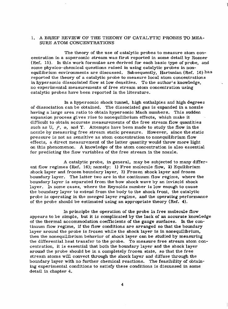
The theory of the use of catalytic probes to measure atom concentration in a supersonic stream was first reported in some detail by Rosner (Ref. 15). In this work formulae are derived for each basic type of probe, and some physico-chemical questions raised in using catalytic probes in nonequilibrium environments are discussed. Subsequently, Hartunian (Ref. 16) has reported the theory of a catalytic probe to measure local atom concentrations in hypersonic dissociated flow at low densities. To the author’s knowledge, no experimental measurements of free stream atom concentration using catalytic probes have been reported in the literature.

In a hypersonic shock tunnel, high enthalpies and high degrees of dissociation can be obtained. The dissociated gas is expanded in a nozzle having a large area ratio to obtain hypersonic Mach numbers. This sudden expansion process gives rise to nonequilibrium effects, which make it difficult to obtain accurate measurements of the free stream flow quantities such as U, p, a, and T. Attempts have been made to study the flow in the nozzle by measuring free stream static pressure. However, since the static pressure is not as sensitive as atom concentration to nonequilibrium flow effects, a direct measurement of the latter quantity would throw more light on this phenomenon. A knowledge of the atom concentration is also essential for predicting the flow variables of the free stream in the nozzle,

A catalytic probe, in general, may be subjected to many different flow regimes (Ref. 16); namely: 1) Free molecule flow, 2) Equilibrium shock layer and frozen boundary layer, 3) Frozen shock layer and frozen boundary layer. The latter two are in the continuum flow regime, where the boundary layer is separated from the bow shock wave by an inviscid shock layer. In some cases, where the Reynolds number is low enough to cause the boundary layer to extend from the body to the shock front, the catalytic probe is operating in the merged layer regime, and the operating performance of the probe should be estimated using an appropriate theory (Ref. 4).

In principle the operation of the probe in free molecule flow appears to be simple, but it is complicated by the lack of an accurate knowledge of the thermal accommodation coefficients of the gauge surfaces. In the continuum flow regime, if the flow conditions are arranged so that the boundary layer around the probe is frozen while the shock layer is in nonequilibrium, then the nonequilibrium behavior of shock layer can be studied by measuring the differential heat transfer to the probe. To measure free stream atom concentration, it is essential that both the boundary layer and the shock layer around the probe should be in a completely frozen state, so that the free stream atoms will convect through the shock layer and diffuse through the boundary layer with no further chemical reactions. The feasibility of obtaining experimental conditions to satisfy these conditions is discussed in some detail in chapter 4.

4

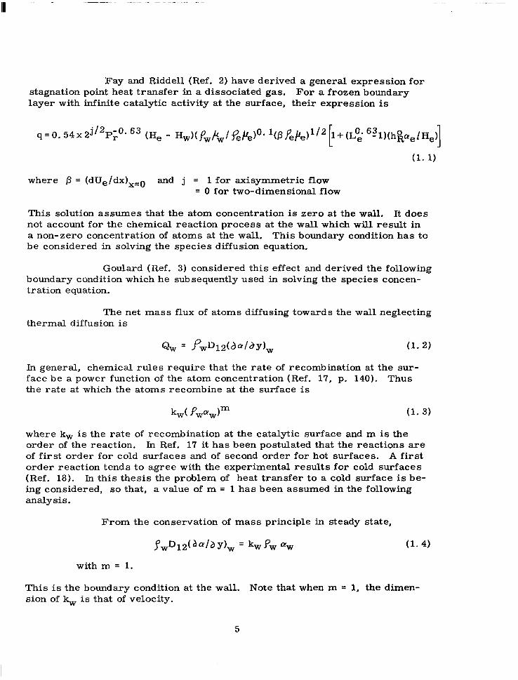
Fay and Riddell (Ref. 2) have derived a general expression for stagnation point heat transfer in a dissociated gas. For a frozen boundary layer with infinite catalytic activity at the surface, their expression is

q = o. 54x 2j’2P-oS 63 r (H e - Hw)(fwkwI f&pe) 0. l(pfepe)1’2 (Lo,’ 6’1)(hgQe/He) 1 (1. 1)

where /3 = (dUe/dxJxZO and j = 1 for axisymmetric flow = 0 for two-dimensional flow

This solution assumes that the atom concentration is zero at the wall. It does not account for the chemical reaction process at the wall which will result in a non-zero concentration of atoms at the wall. This boundary condition has to be considered in solving the species diffusion equation.

Goulard (Ref. 3) considered this effect and derived the following boundary condition which he subsequently used in solving the species concentration equation.

The net mass flux of atoms diffusing towards the wall neglecting thermal diffusion is

Qw = ~wD12(&/J~)w

In general, chemical rules require that the rate of recombination at the surface be a power function of the atom concentration (Ref. 17, p. 140). Thus the rate at which the atoms recombine at the surface is

where k, is the rate of recombination at the catalytic surface and m is the order of the reaction. In Ref. 17 it has been postulated that the reactions are of first order for cold surfaces and of second order for hot surfaces. A first order reaction tends to agree with the experimental results for cold surfaces (Ref. 18). In this thesis the problem of heat transfer to a cold surface is being considered, so that, a value of m = 1 has been assumed in the following analysis.

From the conservation of mass principle in steady state,

fwD12( aa/b yJw = k,x, Pw ow

with m = 1.

This is the boundary condition at the wall. Note that when m = 1, the dimen- sion of ‘sy is that of velocity.

5

It is clear from this equation that no diffused atom can reach the wall if the concentration @w is zero, unless the rate of recombination at the catalytic wall (k,) becomes infinite. The other extreme case of a non- catalytic surface (k,-cO) implies, since cuw is finite, that the net mass flux of atoms towards the wall is zero. Thus, in this case, Q = oe applies throughout the boundary layer.

Using the zero pressure gradient solution for velocity profile (Blasius solution) and the boundary condition given by Eq. (1.4) Goulard (Ref. 3) integrated the species conservation equation for a frozen boundary layer, and obtained the following expression for stagnation point heat transfer.

q = 0.47 x 2 j/2 p -213 r (fiPefe)1’2 He 1 + (Le2’3@-l)(h0, ae/Hej

(1.5) where

G = catalytic efficiency = k,/(k, + S) = rate of recombination at the wall = [2 ‘1/(2-y)] (v/4)

‘/ = No. of atoms that recombine on the wall/unit time/unit area No. of atoms that reach the wall/unit time/unit area

v = is the mean thermal speed

S = diffusion velocity of atoms in the boundary layer

s = 0.47 x 2j/2(p Fe g,P 8c-2/3 9 -l W

p z (dUe/dx)x=o = (2 U,/d) ( Pa/ Ye) 12 - ( Pa/P,)) 1’2 1 041 for h* 03 (infinite catalyticity) (i$->O for &A0 (zero catalyticity)

It is interesting to note that the catalytic efficiency depends not only on kvv but also on flow variables through S. Note also the expression for P=(dUe/dx),,O is the same for axisymmetric and two-dimensional geometries (Ref. 19).

Comparing Eqs. (1. 1 and 1. 5), the only difference between the two is that the heat transfer caused by the diffusion of atoms is multiplied by a factor 0 due to the finite chemical reaction rate at the wall. The slightly different numerical factor is due to the assumption of zero pressure gradient (Blasius solution) in Goulard’s analysis.

Therefore, using the general form of the Fay and Riddel ex- pre s sion, and introducing 8 to take into account a finite reaction rate at the wall, a general equation for stagnation point heat transfer is obtained as

6

q=o.54x2j P- ‘2 ro’ “QHe-Hw)(Pwkv/Pe~~‘48Pe~)1’2 [,+(Lt’ 6%-l)(hg0,/2$ .

The difference in heat transfer between catalytic and non-catalytic surfaces is

[9c- qnc] = 0.54x 2j’2S,o* 6?He-Hw)(fw~w/Pe~P’1(~~pe)1’2(hORaelHeYQc-B,,)

(1.7)

To obtain the maximum difference between qc and qnc, @,, should be small compared to oc. Catalytic gauges are coated with materials such as silver which have a high catalytic efficiency. Silver coated gauges assume values for k, between 1500 to 2000 cm/set (Ref. 11). Also, at hypersonic speeds, S can assume values ranging from 100 to 300 cm/set. Thus, a value of 8, = 0.8 to 0.9 can be expected for silver. A silicon monoxide (SiO) coating behaves as a very good non-catalytic surface to oxygen atom recombination, and it has been established (Ref. 11) that the rate of recombination at the SiO surface can be as low as 1 cm/set. Therefore gnc becomes negligibly small compared to @,, and assumed zero in the present analysis.

Putting one = 0, the general expres,sion for differential heat transfer is given by

kc- qnc] = o. s4 x 2j&;O-63 (He-&)( P,&IP,/&)O* 1(P&@1/2(h$e/He) tic (1.8)

If the boundary layer and shock layer are frozen, the rxe can be replaced by (Ye. In any given run the differential heat transfer (qc- q,,) is measured, by using two gauges (one catalytic and the other noncatalytic) mounted near the stagnation region of a probe (to be called a differential catalytic probe). Then a03 can be estimated from Eq. (1. 8) if all the other flow quantities and Qc are known accurately. Some of the difficulties involved in using Eq. (1.8) and methods of avoiding these will be discussed in the next section.

2. THEORETICAL CONSIDERATIONS OF A SELF- CALIBRATING PROBE

2. 1 Introduction and Assumptions

Estimation of (yo., from Eq. (1.8) is made difficult by the fact that gc has to be determined by a separate and relatively complicated calibration experiment. Also, flow quantities like p, U, k, have to be known accurately to get any meaningful measurements of coo. Several investigators (Ref. 11 and 20) have used glow discharge experiments to determine the surface recombination efficiency r’ of silver (defined in the preceding chapter). In these experiments, a very slow flow (20 to 50 ft/ set) of oxygen was established over a differential catalytic probe and at a given time, R. F. energy was suddenly applied at an upstream position, thereby producing a step function

7

in the degree of dissociation of oxygen gas. When the dissociated column of oxygen arrived at the probe, the differential heat transfer to the probe was measured. The fraction of oxygen dissociated by the RF energy discharge was estimated by a titration experiment. Using the theoretical analysis (Ref. 21) of such a flow over the probe, gc was determined using the measured value of Do0 and the differential heat transfer. No quantitative measurements have been reported by Myerson (Ref. 20) but Hartunian et al (Ref. 11) report a value of YsO. 15 * 15%. To obtain tic, however, the mean thermal speed and the diffusion velocity of the species, which are functions of p, U, T, and /.A of any given gas, have to be known accurately. The values of 9, U, T and paare also necessary to calculate ao, from Eq. (1.8). An accurate estimation

of viscosity of dissociated gases (Ref. 22) is difficult owing to the lack of satisfactory models to describe the intermolecular force potential. The viscosity of gases at low pressures depends also on the density of the gas (Ref. 22). The estimations of p, U, T and )nin hypersonic streams are subject to considerable errors because the chemical state of the gas in the free- stream is not known accurately. These quantities are also affected by large boundary layer growth along the nozzle walls. Thus, use of Eq. (1.8) to estimate (Y~ leads to considerable errors.

In the following sections a method will be presented which not only makes it possible to measure Qic but also avoids the use of 9, U, T and /Lto estimate cum. The principle is to use two differential heat transfer

probes of different geometry in any given run, and to measure the differential heat transfers to both probes. Then 8, can be estimated from a simple expression which is a function of the measured differential heat transfers and the probes diameter ratio. Consequently, (Ye can be estimated using this value of tic and the measured heat transfers.

The following assumptions are made in the analysis.

1) The rate of recombination (k,) at the two catalytic gauges is the same (i.e. kw3 = kw2).

2) An uniform core of free stream flow exists in a given plane of the test section, so that the effects of lateral gradients in the flow on the measured heat transfers are negligible (see Sec. 5. 3).

The first assumption is based on the fact that the heat transfer gauges were coated with the same catalytic material under identical conditions.

8

2.2 Boundary Layer Regime

2. 2. 1 Combination of Axisymmetric and Two-dimensional Probes

Equation (1.8 )-gives the genersl expression for the differential heat transfer. Therefore, if two differential heat transfer probes (one axisymmetric and the other two-dimensional) are mounted side by side in a hypersonic uniform stream and the differential heat transfer to both models is measured simultaneously, then the expressions for the differential heat transfer are:

(i) Axisymmetric flow

L 3 qc’ qnc = 0.76.S, -O’ 63(He- Bw)(P,pw/Pe)h)“’ 1(83/‘e&)1’2(h2&He)Gc3

3 (2.1) where

0 c3 = kJ(k,+S3)

S3=6.76 (P3fe&) 1/2s-O. 63

c P’ -I

03 = (2U,/d3) [(p,If&) f2-l Pa/P,)]] 1’2

(ii) Two-dimensional flow

Cq,- qnc]; 0. 54 S’-,O’ 63(He-%)( fwk$/ fe&)O’ ‘(P2 P,~e)1’2(h~~~/He)@c2 (2.2)

where 0 c2 = k,/b.,,,+S2)

s2 = 0.54 (P2pePe)1’2 go’ s3p,-1

132 = (2U,/d2) [( P,/Pe) f2-( ?mlPe)]] 1’2

Dividing Eq. (2. 1) by Eq. (2. 2) yields

1 (% - %x)3

II

(qc- qnc12z $2 = (2 83/P2)1’2 (C&,/~,,)

S2, S3, and B,,. ‘k3 are interrelated and can be expressed as

(S3lS2) = (2P3/P2) lJ2 = (2d2/d3)l12

0cpc2 = 0c3 +.(l - 0c3)(dg/2d2)1’2

0 c2

= ‘$,, / bc3 + (1 - ‘&3Nd3/2d2)1’2 L 1 Using Eqs. (2.4) and (2.5) Eq. (2.3) can be expressed as

(2. 3)

(2.4)

(2.5)

(2.6)

9

0 c3

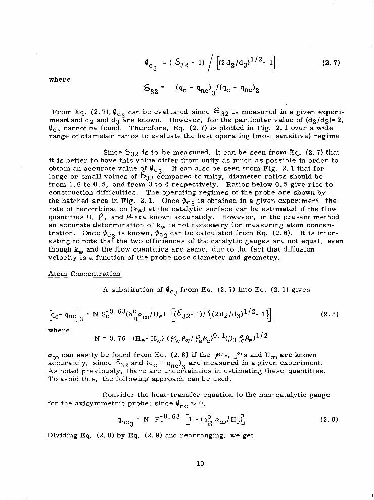
= ( 632 - 1) 11% 1 1 (2.7)

where S 32 = (qc - 9,c)3/(9c - qnc)2

From Eq. (2.7), flc3 can be evaluated since 6 32 is measured in a given experi- meadand d2 and d3 are known. However, for the particular value of (d3/d2)= 2, 0 c3 cannot be found. Therefore, Eq. (2.7) is plotted in Fig. 2. 1 over a wide range of diameter ratios to evaluate the best operating (most sensitive) regime.

Since 632 is to be measured, it can be seen from Eq. (2. 7) that it is better to have this value differ from unity as much as possible in order to obtain an accurate value of tic,. It can also be seen from Fig. 2. 1 that for large or small values of 632 compared to unity, diameter ratios should be from 1.0 to 0. 5, and from 3 to 4 respectively. Ratios below 0. 5 give rise to construction difficulties. The operating regimes of the probe are shown by the hatched area in Fig. 2. 1. Once QC3 is obtained in a given experiment, the rate of recombination (k,) at the catalytic surface can be estimated if the flow quantities U, p, and Fare known accurately. However, in the present method an accurate determination of k, is not necessary for measuring atom concentration. Once 8,, is known, oc2 can be calculated from Eq. (2. 6). It is interesting to note that the two efficiences of the catalytic gauges are not equal, even though k, and the flow quantities are same, due to the fact that diffusion velocity is a function of the probe nose diameter and geometry.

Atom Concentration

A substitution of tic3 from Eq. (2. ‘7) into Eq. (2. 1) gives

[qc- qnc] 3 = N Si”* 63(h>,/He) p6,2- l)/ 1(2d2/d3)1’2- 111

where N = 0.76 (He- Hw) (pwPw/ P,Pe)O’ ‘(B3 P,&)1’2

(2.8)

(Ye can easily be found from Eq. (2.8) if the p s, B’S and U, are known accurately, since A32 and (qc - qnc)3 are measured in a given experiment. As noted previously, there are uncertainties in estimating these quantities. To avoid this, the following approach can be used.

Consider the heat-transfer equation to the non-catalytic gauge for the axisymmetric probe; since gnc 5 0,

qnc 3 = N ,;Om6” [l - (h”R +,/Hefl (2. 9)

Dividing Eq. (2.8) by Eq. (2. 9) and rearranging, we get

10

h& “a/He = 1 / k + tic3 Le O’ 63 \qnc’(qc-qnc).j 3-J (2.10)

where dc3 is estimated from the measured values using Eq. (2.7). Therefore,

(2.11)

In Eq. (2.11) all the quantities are measured except the Lewis number and the total enthalpy. The Lewis number (L,) is usually taken as a constant for a given temperature (T,), and He can be obtained fairly accurately from the reservoir conditions in a given hypersonic shock tunnel and the assumption that He = Ho. A method of estimating reservoir enthalpy is outlined in Chapter 3. Consequently, by using this approach it is not necessary to know either the flow quantities or the rate of recombination (kvv) at the catalytic surface in order to compute the free stream atom concentration.

An expression similar to Eq. (2. 11) can also be derived by using heat transfer equations for the two-dimensional model, and a,, is estimated by using measurements of heat transfer to the two-dimensional model. The equation for (Ye is,

iqnc’(qc- qnc) 3 23 (2. 12)

where Oc2 is calculated from Eq. (2. 6).

This calculation serves as a check for the measurement of (Ye.

2. 2. 2 Combination of Geometrically Similar Probes

A combination of either two axisymmetric, or two, two- dimensional differential catalytic probes could also be used to measure catalytic efficiency and atom concentration. For example, considering two axisymmetric probes the expressions for differential heat transfer could be written from the general Eq. (1.8), and are:

where s stands for smaller probe.

= 0.76 S,” 63 (He- Hw)( fwfi,/ fef’e,O* ‘(P31 &pef ‘2(h~,/He)Bc31

where 1 stands for the larger probe, where 63s, 631, QC3s and gc31 are (2.14)

similar to expressions defined in Eq. (2. 1). Dividing Eq. (2. 13) by Eq. (2. 14), we have

(qc- qnc)3s ’ (9, - qnc)31z~3sl = (~3s’~sl)1’2(~c3s’Qc31)

11

~-.. ------.-. .-... -. . . . . . . . .,. m. , , . .

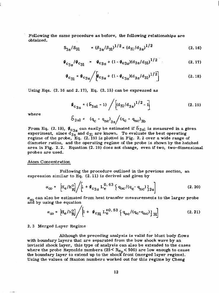
Following the same procedure as before, the following relationships are obtained.

s3sJs31 = (P3s’1331) ‘I2 = (d31’d3s)1’2

0c3s/0C31 = Ocgs + (l- 0c3s)(d3s/d~1)1’2

0 c31

=0 c3s + (I- 0c3s)(d3s’d31~1’2 3

(2. 16)

(2.17)

(2. 18)

Using Eqs. (2.16 and 2.17), Eq. (2.15) can be expressed as

0 c3s = ( s3sl - 1) (2.19)

where 6 3d = (9, - qnc)as

/ (qc - qnc)CJb

From Eq. (2. 19), acgs can easily be estimated if 63sl is measured in a given experiment, since dgs and d31 are known. To evaluate the best operating regime of the probe, Eq. (2. 19) is plotted in Fig. 2. 2 over a wide range of diameter ratios, and the operating regime of the probe is shown by the hatched area in Fig. 2.2. Equation (2. 19) does not change, even if two, two-dimensional probes are used.

Atom Concentration

Following the procedure outlined in the previous section, an expression similar to Eq. (2.11) is derived and given by

aoo = + ‘&3s LE. 63

(ro3 can also be estimated from heat transfer measurements to the larger probe and by using the equation

2.3 Merged Layer Regime

(2.21)

Although the preceding analysis is valid for blunt body flows with boundary layers that are separated from the bow shock wave by an inviscid shock layer, this type of analysis can also be extended to the cases where the probe Reynolds numbers (25< Rep < 500) are low enough to cause the boundary layer to extend up to the shock front (merged layer regime), Using the values of Stanton numbers worked out for this regime by Cheng

12

(Ref. 4), and assuming the similitude considerations of heat transfer in the boundary layer regime (Ref. 23) to apply in the merged layer regime, a method of applying the self-calibrating technique in the merged layer regime is presented below.

The Stanton number corresponding to the heat transfer due to convection is defined as

(2.22)

where

‘e =He eR - a ho is the frozen total enthalpy at the edge of the boundary layer or

qk: ~kj&Um(~e- s) (2. 23)

Similarly, the contribution to the total heat transfer due to atom diffusion can be written as

%i= sd fm u, hg be - awl (2. 24)

where Std is the Stanton number corresponding to the heat transfer due to atom diffusion.

Then the total heat transfer is

(qk + CQ) = q = stk PO0 U&H, - s> + sd f& U, hg (Qe - 0~) (2.25)

From similitude theory, we assume that the Stanton number Std is obtainable from the Stanton number Stk by replacing the Prandtl number by the Schmidt number. This is asymptotically exact for the low speed, frozen flow case when the free stream atom concentration is small compared to unity (Ref. 23).

Jn the boundary layer regime the functional form of stk is given bY

(Stka.l. = pr -O* 63 fq(U~~poOs da f’e> &I (2.26)

Using the similitude concept,

(std)b.l. = ‘c -O* 63 fq (U,a Pas ds f’es /+I (2.27)

Therefore, (2.28)

Let us assume* Eq. (2.28) holds good also in the merged layer regime. Then

* This assumption can be justified in the following manner. Considering the first order analytical solution of Cheng’s theory (Ref. 4) in the merged layer regime, an expression for Stk similar in functional form to Eq. (2.26) can be obtained. This provides the basis to write (Stk)m.l= P~0:~3&(U03, pa, d, pe, Fe). Then US- ing the similitude considerations (St

-0.69 Therefore (Sk),, 1. kStd)m. 1. =L, )ml. = SC ’ fn2 (U, pmj d, Pe*&)* .

13

using Eq. (2.28) in Eq. (2.25) the total heat transfer reduces to

q= stk &, uoo I (ii, - s) + LE’63 hi (Qe - 0,)

I W.29)

The stagnation point heat transfer theory by Cheng (Ref. 4) was worked out for a perfect gas with constant specific heats, so that the solution for Stanton numbers in his analysis corresponds to stk. This is the main motivation in express- ing the total heat transfer (Eq. 2. 29) as a function of Stk.

In Eq. (2.29) ow can be expressed in terms of Cre by using the boundary condition at the wall (Eq. i. 4)

kw aw &, = ?wD12 @day), (2.30)

But by the definition of D12 and hg

(2.31)

Therefore

Pw Qw & = q&o, = std f&, u, be - Qw)

Using Eq. (2. 28)

f-W % % 0.63

= Sk L, j+~, u, be- Qw) (2. 32)

Solving for cyw from Eq. (2.32)

@w = @e/[l+b/(sk Lg. 63fa uafw-‘)] (2. 33)

Using the expression for Stk from boundary layer theory the term stk L,o’ 63 Pm ~CDPW- l reduces to 0.54x 2112 fw-l ScZo* 63(p gpe)‘j2 which is exactly the diffusion velocity S defined in Eq. (1. 5). Therefore the expression for diffusion velocity in the merged layer regime is Stk L&s 63 &, TJ,y),- 1 Using the symbol S for diffusion velocity as before, Eq. (2.33) reduces to

aw=ae/[l+kw/S] (2. 34)

Where, 0.63 S=StkLe PO3 %I fw- l

Using the same definition for efficiency @ = k,/(k,+ S) as before,

(kw/S) = @ / (l- 0) and k + kw/S] = l/(1 - 0)

Thus, the boundary condition at the wall reduces to

CYw = (1 - 0) (ye (2. 35)

14

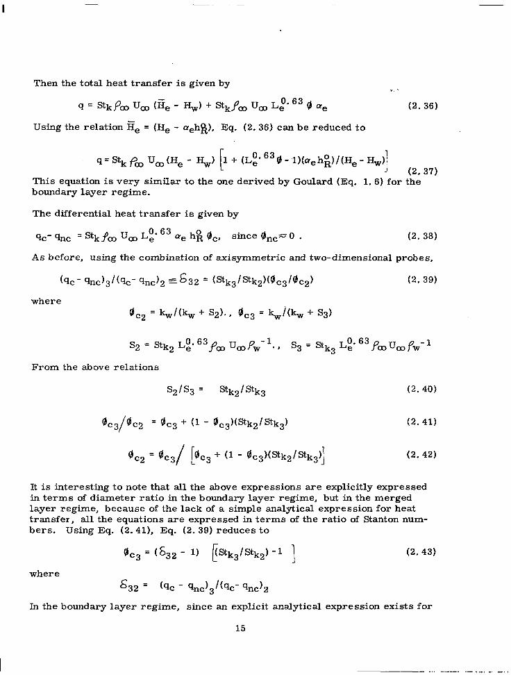
Then the total heat transfer is given by

Cl = skfa ‘J, C& - H&I + Stk,?a U, J-J:’ 63 0 Qe

Using the relation Ee = (He - oeh&), Eq. (2.36) can be reduced to

T. .

(2.36)

q=s,f&, U&H, - I&> p + (Lt.63 0 - l)(aehg)/(He - Hw): (2.37)

This equation is very similar to the one derived by Goulard (Eq. 1.6) for the boundary layer regime.

The differential heat transfer is given by

qc- qnc = Stkfao u, Le ” 63 eye hg &, since C&s 0 . (2. 38)

As before, using the combination of axisymmetric and two-dimensional probes,

(qc- 9nc)3/(9c- qnc)2 =fJ32 = (stk3/~k.$t0c3/0c2)

where 0 c2 = &/(k, + S2). , UC3 = h/Ck, + S3)

(2. 39)

0.63 % = Stk2 Le f&, &,p,% S3 = Stk3 L0,-63&,um~w-1

From the above relations

S2lS3 = Stk2 / Stk3 (2.40)

gc3/oc2 = 8c, + (1 - 0c3)(Stk2/%3) (2.41)

0 c3 + (1 - 0c3)(~k2/stk3)] (2. 42)

It is interesting to note that all the above expressions are explicitly expressed in terms of diameter ratio in the boundary layer regime, but in the merged layer regime, because of the lack of a simple analytical expression for heat transfer, all the equations are expressed in terms of the ratio of Stanton numbers. Using Eq. (2.41), Eq. (2. 39) reduces to

0 ~~~(632~ 1) r (stk3/~k2) - 1 ] (2.43)

where s 32 = (qc - 9,c)3/(9C- qnc)2

In the boundary layer regime, since an explicit analytical expression exists for

15

Stanton numbers, the ratio of Stanton numbers works out to be

(~k3/~k2) = (2 d2/d3) 112 (2.44)

Thus, Eq. (2.43) is similar to Eq. (2.7) which is derived for the boundary layer regime.

In order to compute gc3 from Eq. (2.43) the ratio of Stanton number s should be known. This ratio was obtained from Ref. 4. In this reference analytical solutions with first and second order approximations are given. How- ever, these solutions are implicit and not simple in mathematical form. Also these are not exact. So it was decided to use the values of Stk obtained by numerical computation.

.Tn Ref. 24 the Stanton numbers are computed for axisymmetric and two-dimensional flow configurations by using the theory of Ref. 4, and are plotted for a wide range of probe Reynolds numbers (25<Rep <lOOO). These values were used to compute the ratio of Stanton numbers. The ratios of (Stk3/Stk Fig. 2. 3 ?

) obtained for the values of (dg/d2) = 0. 5, 1.0 and 4.0 are plotted in or Reynolds number range 20 LRepC 1000. The Stanton number ratio

increases slightly from boundary layer value and approaches a constant value as the Reynolds number decreases. The Stanton number ratio is independent of Reynolds number in the boundary layer regime. This is not true in the merged layer regime as evident from Fig. 2.3. However, the maximum difference from the boundary layer value is about 5% (Fig. 2. 3). If one is con- tent to use an average vslue throughout the low Reynolds number range, then the maximum error will be about 2.5%. Using this value as a correction factor, the ratio of Stanton numbers can be expressed in an analytical form in the merged layer regime as,

since

I Stkg/Stk2

3 m 1 = 1.025

* .

(sk3’stk2)b. 1.

(2 d2/d3)1’2 (2.45)

= (2 d2/d3)lj2

and 0 c3 = (‘32- l)/ b. 025 (2d2/d3)1’2-l] (2.46)

Thus the self-calibrating technique can be used even in the merged layer regime.

Atom Concentration

Following the procedure outlined in Sec. 2.2, an expression identical to Eq. (2. 11) can be derived. In other words the expression for computing atom concentration does not change.

16

3. EXPERIMENTAL FACILITY AND ITS CALIBRATION

3.1 Shock Tube, Nozzle System and Test Section

After having postulated a technique of measuring the catalytic efficiency and the atom concentration simultaneously in any single experiment, it was considered important to test the practical feasibility of this technique. Consequently this technique was used to measure the free- stream atom concentration in the UTAS 11 inx 15 in Hypersonic Shock Tunnel test section.

This tunnel is of the “reflected type” and is capable of operating at moderately high stagnation enthalpies necessary for this type of experiment. The instrumentation, calibration and an outline of the problems encountered in the calibration of this shock tunnel with some of the solutions are presented in some detail in UTIAS Technical Note No. 91 (Ref. 25).

The UTIAS 11 in. x 15 in Hypersonic Shock Tunnel consists of two main parts, the shock tube driver and driven sections, and the nozzle system, dump tanks and test section. The general layout of this facility is shown in Fig. 3. 1. The shock tunnel and its associated instruments are shown in Fig. 3. 2. The combustion driver of the shock tube is 2 in. x 2 in. cross section and 7 feet long and is installed in a block house for the safety of operating personnel. The channel is also 2 in. x 2 in. cross section and 15 feet 5 in. long and is coupled to the nozzle system by a coupling nut which has two instrument ports l- l/4 in. from the entrance to the primary nozzle, A Mylar diaphragm 0.0002 in. thick was installed at the entrance to the primary nozzle in order to isolate the tunnel test section and dump tanks from the channel section.

During the calibration of the shock tube, only quantities essential for the operation of a reflected-type shock tunnel were measured. Kistler #603 and #605 pressure transducers were used to measure the pressure time-history immediately after shock reflection. The transducer was mounted in the coupling nut l-1/4 in. upstream of the nozzle entrance. These transducers were used in conjunction with Kistler charge amplifiers and a Tektronix 565 oscilloscope. Two barium titanate pressure transducers (BD-25) were mounted on the shock tube walls one foot apart, the second gauge being 11 in. upstream of the nozzle entrance. These gauges have a response time of less than 1 psec. The outputs from these gauges were amplified in a dual channel pulse amplifier and used to start and stop a ‘R.ACAL’ time interval counter which has a counting accuracy of f 1 +sec. Since the shock speed was measured between stations one foot apart adjacent to the end of the shock tube, the attenuation effects over this interval were assumed negligible.

To produce uniform combustion along the length of the driver and to minimize the possibility of detonation in the driver, a stoichiometric mixture

17

of hydrogen and oxygen diluted with helium was ignited by instantaneous heating of a tungsten wire (which was mounted along the center line of the driver) over its entire length, A discharge from the capacitor bank (50 /.LF, 3000~) passing through the wire (energy of about 225 joules or 32 joules/ft. of wire) heated the wire impulsively to a bright read and was sufficient to ignite the mixture. A thorough discussion of various ignition methods for combustion drivers is given in Ref. 26.

The diaphragms used were of stainless steel discs of 6 in. dia and of thicknesses 0.018 in, 0.029 in, and 0.037 in. Prior to their use, two grooves at right angles were scribed on all the diaphragms to a depth which controlled the bursting pressure. By maintaining tight quality control on depth of cut, very good repeatable operation was achieved (shock Mach number variation was within 2% between runs).

The nozzle system was employed in order to expand the gas at the end of the shock tube, which was at high temperature and high pressure, to hypersonic Mach numbers. It consists of three sections, as illustrated in Fig. 3.3. The first expansion is provided by a two-dimensional convergent-divergent nozzle with a contraction area ratio of 10.7 to 1, and an expansion area ratio of 49 to 1. The height of the nozzle is l- l/2 in. throughout its length, the width increasing from 0.25 into 12.25 in.(yielding a Mach number MS 6.0). The second expansion (corner expansion) is provided by a deflection plate at an angle of attack of - loo (further raising Mz~. 0) and in the plane of the primary nozzle. This plate serves the important purpose of preventing any particles such as diaphragm fragments from entering the terminal nozzle. While the supersonic flow is turned, the particles go straight through without going into the terminal nozzle. Theyfall into the receiving tanks. The terminal nozzle, inclined at -100 to the horizontal is mounted at the end of the deflection plate and is a straight- sided two-dimensional nozzle with an included angle of 15O (giving a final M x 15.0 to 17.0). The test section flow Mach number can be varied by chang- ing the height of the terminal nozzle entrance, the width remaining constant at 11 in. However, for all the experiments reported in this thesis, the height of the terminal nozzle entr.ance was kept at 0.4 in.

The final test-section, which is 11 in. wide and 15 in. high is the end of the terminal nozzle (Fig. 3. 3). Testing was done at this station and also at 6 in. upstream from this station. The test gas which bypasses the nozzle system flows into two receiving tanks on either side of the tunnel. The test section is followed by a 13 foot long receiving tank, to delay the arrival of shock reflected from the end of the receiving tank.

In order to minimize the nozzle starting time, the nozzle system and dump tanks were evacuated to nearly 2 /LHg. The vacuum system consists of a mechanical pump (a CVC type E-135) with a pumping speed of 80 CFM, and it lowers the pressure in the tunnel to about 50 PHg. Then the diffusion pump (a CVC type PMC-1440 and a CVC water cooled chevron ring baffle, type BCR-U installed at the inlet of the diffusion pump to prevent pump oil vapour from getting into the tunnel) takes over the evacuation at low pressures. A manually operated

18

quick-acting gate valve separates the tunnel from the diffusion pump during tunnel operation. The pressure inside the tunnel was measured by a Pirani gauge (type GP-145) and Stokes McLeod gauge. The complete system was evacuated to the order of 2 /AHg in about 20 minutes.

The channel section of the shock tube was evacuated to about 50 p Hg by using the same mechanical pump. The driver section was evacuated by a small mechanical pump located inside the block house.

3. 2 Reservoir Conditions

In hypersonic shock tunnels, high temperature and high pressure gases are expanded in a system of nozzles with large area ratios to achieve hypersonic Mach numbers. If the reservoir temperature is high enough to cause any diatomic gas to dissociate before it is expanded in the nozzle, then there will be recombination between the atoms as the gas expands along the nozzle. This gives rise to non-equilibrium effects in the nozzle flows. However, if the reservoir pressures are sufficiently low, then the recombination becomes negligible very early along the nozzle (frozen flow) so that the test flow contains a considerable amount of dissociated species. A large dissociation of the test gas in the reservoir and early freezing in the noz.zle are ,essential to obtain measurable quantities of atomic species in the test section flow. A brief review of the theoretical analysis of non-equilibrium flow phenomenon in the UTIAS hypersonic shock tunnel nozzle system taken from Ref. 14 is given in the Sec. 3. 3.

Low reservoir pressures and high reservoir temperatures (see Table 3.1) were obtained by operating the shock tube at initial channel pressures from 5 mm to 25 mm of Hg and incident shock Mach numbers from 9.6 to 11.7. Oxygen was used as the test gas because of its low dissociation energy. The tailored-interface technique (Ref. 25) was employed to get sufficient testing time. The tailored shock Mach numbers attainable from constant volume combustion are limited by attenuation effects (Ref. 25). It has been demonstrated in Ref. 27 that for the case of equal specific heat ratios of driver and driven gases and for perfect, inviscid gases, the interface, if tailored initially, remains tailored, whether the shock is attenuated or accelerated. Therefore, tailoring shock Mach numbers greater than those attainable by constant volume combustion are possible, if the incident shock Mach number that is tailored initially is accelerated by some technique. This can be achieved (Ref. 25) by using a combination of constant-volume and constant-pressure combustion in the driver.

The above technique is quite simple. The driver volume was filled with stoichiometric mixture of oxygen-hydrogen diluted with helium, but to a pressure such that the diaphragm would burst before the peak pressure was reached. The pressure which is increasing in the ‘quasi-steady’ region of the expanded driver accelerates the shock as it moves down the tube until combustion is complete. Afterwards, the shock stops accelerating and begins to decelerate (or attenuate) in the usual manner. The above principle was used in the 2 in. x

19

2 in. shock tube to obtain tailored shock Mach numbers as high as 10. For a detailed discussion Ref. 25 may be consulted.

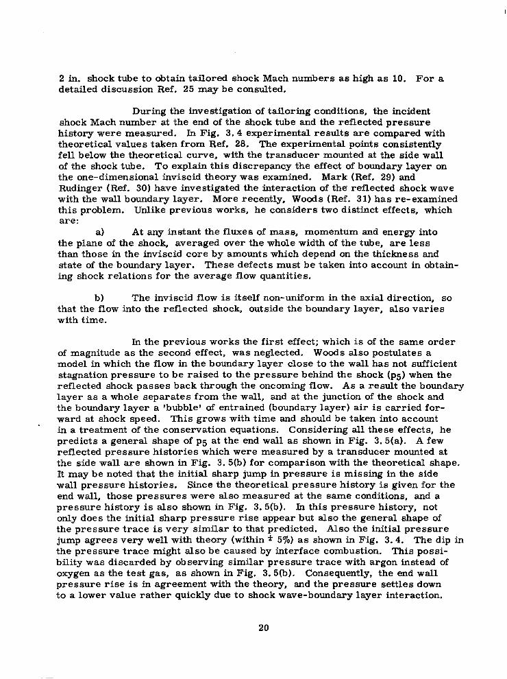
During the investigation of tailoring conditions, the incident shock Mach number at the end of the shock tube and the reflected pressure history were measured. In Fig. 3.4 experimental results are compared with theoretical values taken from Ref. 28. The experimental points consistently fell below the theoretical curve, with the transducer mounted at the side wall of the shock tube. To explain this discrepancy the effect of boundary layer on the one-dimensional inviscid theory was examined. Mark (Ref. 29) and Rudinger (Ref. 30) have investigated the interaction of the reflected shock wave with the wall boundary layer. More recently, Woods (Ref. 31) has re-examined this problem. Unlike previous works, he considers two distinct effects, which are:

a) At any instant the fluxes of mass, momentum and energy into the plane of the shock, averaged over the whole width of the tube, are less than those in the inviscid core by amounts which depend on the thickness and state of the boundary layer. These defects must be taken into account in obtaining shock relations for the average flow quantities.

b) The inviscid flow is itself non-uniform in the axial direction, so that the flow into the reflected shock, outside the boundary layer, also varies with time.

In the previous works the first effect; which is of the same order of magnitude as the second effect, was neglected. Woods also postulates a model in which the flow in the boundary layer close to the wall has not sufficient stagnation pressure to be raised to the pressure behind the shock (~5) when the reflected shock passes back through the oncoming flow. As a result the boundary layer as a whole separates from the wall, and at the junction of the shock and the boundary layer a ‘bubble’ of entrained (boundary layer) air is carried for- ward at shock speed. This grows with time and should be taken into account . in a treatment of the conservation equations. Considering all these effects, he predicts a general shape of p5 at the end wsll as shown in Fig. 3.5(a). A few reflected pressure histories which were measured by a transducer mounted at the side wall are shown in Fig. 3.5(b) for comparison with the theoretical shape. It may be noted that the initial sharp jump in pressure is missing in the side wall pressure histories. Since the theoretical pressure history is given for the end wall, those pressures were also measured at the same conditions, and a pressure history is also shown in Fig. 3.5(b). In this pressure history, not only does the initial sharp pressure rise appear but also the general shape of the pressure trace is very similar to that predicted. Also the initial pressure jump agrees very well with theory (within f 5%) as shown in Fig. 3.4. The dip in the pressure trace might also be caused by interface combustion. This possibility was discarded by observing similar pressure trace with argon instead of oxygen as the test gas, as shown in Fig. 3.5(b). Consequently, the end wall pressure rise is in agreement with the theory, and the pressure settles down to a lower value rather quickly due to shock wave-boundary layer interaction.

20

The reservoir temperature and pressure are needed to calculate flow quantities along the nozzle centre line. Also, other reservoir conditions such as equilibrium atom concentration, enthalpy and density can be obtained if the reservoir temperature and pressure are known (see Sec. 3.3). In every run incident shock speed at the end of the shock tube and reservoir pressure (with gauge mounted in the side wall of the shock tube l-1/4 in. from the nozzle entrance) were measured. Since it is difficult to measure temperatures of the order of 5000°K, a quasi theoretical-experimental procedure was used to evaluate the reservoir temperature.

In Ref. 28 shock tube parameters for oxygen are computed taking into account the real gas effects and are tabulated up to incident shock Mach numbers of 12. These values are considered quite accurate. The reservoir temperature (To) and pressure (PO) corresponding to the measured incident shock Mach number were obtained from these tables. The measured reservoir pressure served as a check. However, the measured pressure was less than the theoretical value due to the boundary layer interaction as already discussed. Also slight over tailored operation was used in some cases so that the pressure history increased with time (see Fig. 3.4). Thus the measured pressure was used as the reservoir presL.ure and the reservoir temperature obtained from tables (Ref. 28) was corrected for the preceding effects by a method outlined below.

The chemical state of the gas in the reservoir, throughout the range of temperatures and pressures used in this work, can be considered to be in equilibrium (Ref. 28). Consequently, the reservoir temperature, corresponding to the ratio of the measured to the theoretical reservoir pressure, can be obtained from a Mollier chart. However, the following analytical method was used to correct reservoir temperature. This method is based on the fact that the difference between the measured and theoretical reservoir pressure was small (in the order of 10 to 15%).

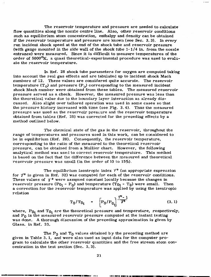
The equilibrium isentropic index Y* (an appropriate expression for ‘J* is given in Ref. 32) was computed for each of the reservoir conditions. These values of y* were assumed constant locally because the changes in reservoir pressure (Pot - PO) and temperature (Tot - TO) were small. Then a correction for the reservoir temperature was applied by using the isentropic relation

To/Tot = [ 1 po/pot % (3.1)

where, Pot and Tot are the theoretical pressure and temperature, respectively, and PO is the measured reservoir pressure computed at the instant testing was done. A thorough discussion of the preceding approximation is given by Glass. in Ref. 33.

The PO and TO values obtained by the preceding method are given in Table 3. 1, and were also used as input data for the computer program to calculate the other reservoir quantities and the free stream atom concentration in the test section (Sec. 3. 3).

21

3.3 Nonequilibrium Nozzle Flow Calculations

At present expansive flows of reacting gases are calculated either by considering the, instantaneous equilibration of vibration with trans- lational and rotational modes and allowing for dissociational non-equilibrium (Refs. 32 and 34). or by considering dissociational and vibrational nonequilibrium to be coupled processes (Ref. 35). The dissociation-recombination rate constants usually used are those determined from analyses or experiments under equilibrium conditions. It has been recently shown that the equilibrium rate constants and vibrational relaxation times so determined will have to be modified. Recent experiments on the vibrational relaxation of undissociated nitrogen in nozzle expansion flows appear to indicate that the measured vibrational relaxation times are shorter than those calculated by using the classical Landau-Teller model for normal shock waves (Ref. 36).

Thus, it was decided to set up a more realistic gas model to take into account all these factors and to estimate the free-stream atom concentration in the UTIAS Hypersonic Shock Tunnel nozzle so that the estimated atom concentrations could be compared with the measured values.

A complete discussion of the flow model used, non-equilibrium thermodynamics and the details of coupling between vibration and dissociation are published in a UTIAS Report (Ref. 14) by Tirumalesa. One dimensional steady flows of pure dissociated oxygen through the nozzle were computed by numerical integration of governing equations by fourth-order Runga-Kutta method on an IBM 7090 Computer at the Institute of Computer Science, University of Toronto.

The reservoir pressure and temperature determined by the methcd outlined in Sec. 3. 2, were used as input quantities to the programme developed for nonequilibrium nozzle flows calculations (Ref. 14). Before the nozzle flow calculations begin, the programme calculates other equilibrium reservoir conditions such as CY~, p. and Ho. These values are tabulated in Table 3.1. From non-equilibrium calculations in the primary nozzle, it was found that the atom concentration froze completely in the primary nozzle, consequently, this is the value expected in the test section free-stream (a,). The (Y~ values for all the reservoir conditions so obtained are also given in Table 3. 1.

To study the effect of the vibrational relaxation time on the final test section dissociation mass fraction these values were calculated for three values of cv, namely.

t’ = -r, expansion/ & normal shock = 1.0, 0. 1 and 0.05

It was found that there is a considerable difference between values of ao, for

ZV = 1.0 and 0.05 at low reservoir pressures or higher oo. However, no noticeable difference was found between the values of (Ye for rv = 0.1 and 0.05.

22

Thus, the value of ao, corresponding to t’ = 1.0 and 0.05 are given in Table 3.1 and these values are compared with the measured values in Table 5.2. All the values given in the Table 3.1 were computed using coupled, perferential dissociation model giving a higher efficiency for dissociation from higher vibrational levels. For further discussion of vibrational and dissociational relaxation lengths, Ref. 14 may be consulted.

3.4 Test Section Flow Calibration

Center-line pitot-pressure surveys along the vertical and horizontal centerlines at the 11. in.x 15. imstation and at one foot upstream were conducted to determine the flow uniformity in the nozzle. A pitot rake with three probes was designed to accommodate the Kistler #701A pressure transducers. The pitot probes were also mounted in an off-set position (Fig. 3.6) so that pitot pressure measurements were done at many points along both centrelines. Operational problems such as pyro-electric effects, vibration and pitot probe hole size effects, which are very severe at low pitot pressures and high stagnation temperatures, were investigated in detail and are reported in Ref. 25. The complex problem of nozzle starting process and its severe effect on testing time was investigated in some detail in Ref. 25. The pitot pressure distributions obtained at the 11 in. x 15 in. station along the .ll in. and 15 in. centrelines are shown in Figs. 3.7 and 3.8 respectively. The reservoir condition for these surveys was MS = 9.6, channel pressure pl = 25 mm Hg, PO = 40.0 atms, To = 4600°K, nozzle evacuation pressure = 10 FHg.

It can be seen that the boundary layer along the vertical walls is relatively thin and the “core” along the 11 in. centreline is reasonably uniform and has a width of about 8 in. However, the core along the 15 in. centreline seems to be very small (less than 1.5 in). It has been stated by Hertzberg (Ref. 37) that this distribution is similar to that which was found in this very test section when it was used at Cornell Aeronautical Laboratory, and that this is probably due to the final nozzle not skimming away the boundary layer which grows in the primary nozzle and along the deflection plate. The small uniform core along the 15 in. centreline (if it is due to boundary growth along the walls) cannot be explained because the boundary layer growth along the 11 in. centreline is rather small compared to the one along the 15 in. centreline. Since the flow expands only in the 15 in. plane, there-might be separa- tion (typical of some low Reynolds number nozzle flows) along the walls in this plane. However, in all the tests conducted to measure free-stream atom concentration the catalytic probes were mounted along the 11 in. centreline (see Sec. 5.3). The test section flow Mach numbers were estimated using measured pitot pressures. They varied from 15. 3 to 16.9. This variation is due to change in the frozen ratio of specific heats at different reservoir conditions. The pitot profiles obtained at one foot upstream of 11 in. x 15 in. station were similar to the ones shown in Figs. 3.7 and. 3.8. It may be seen that additional probing will be required to determine the factors leading to such nozzle flows as well as its characteristic properties.

23

I / : ‘!’ ,, . ( / j : ,; ,,; .-‘:I, --r :, .‘C’ ‘. ‘!. , L”>,.’ ‘, (‘I,. , .., _ ‘.,

The wall.static pressures in the test section were also measured at different reservoir conditions. The pressure transducers used were of the type PZT-50- 12-AC made of lead zirconium titanate crystals and these have been designed to measure pressures as low as 0.002 psi. For complete details Ref. 25 may be consulted. These transducers were mounted in the side wall (Fig, 3.6) of 11 in. x 15 in. test section. Using the measured static pressures and frozen ratio of specific heats test section flow Mach numbers were also computed. These were slightly different from those obtained from the pitot pressure measurements. This may be due to the effect of wall boundary layer on the measured static pressure. However, these values are not necessary for either computing or measuring CQ-, in the test section.

The test section flow Mach number was also computed independently by using the relation between the flow Mach number and the area ratio for a perfect gas. In the above computation an effective test section area ratio was used which was determined from the pitot pressure profiles. The flow Mach number obtained by this method compared reasonably well with those obtained from pitot and static pressure measurements. The above check was done to clear the doubt whether the small uniform flow core in the test section could produce the flow Mach numbers that are in question.

4. DESIGN CONSIDERATIONS OF CATALYTIC PROBES

4.1 Introductory Remarks

Iu the continuum flow a bow shock will be formed around the nose of a probe when placed in a hypersonic stream. The high shock strength converts a large part of the free stream kinetic energy into thermal energy so that the inert modes of the gas are likely to equilibrate inside the shock layer. Furthermore, recombination tends to occur inside the boundary layer. Therefore, if the probe is to measure the free-stream atom concentration ahead of the bow shock, experimental conditions have to be such that there will be no further dissociation in the shock layer and recombination in the boundary layer that is a frozen shock layer and a frozen boundary layer exists.

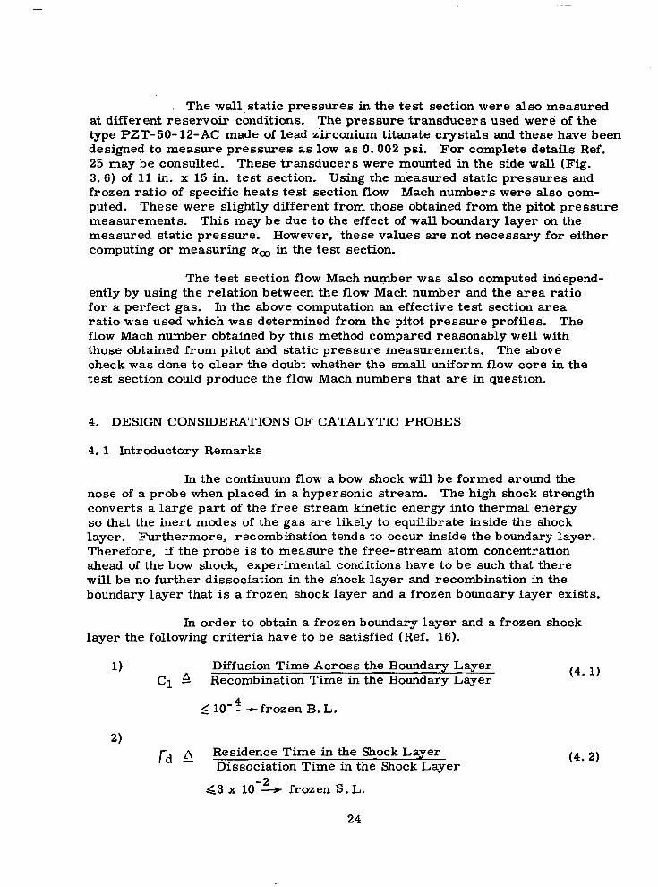
In order to obtain a frozen boundary layer and a frozen shock layer the following criteria have to be satisfied (Ref. 16).

1) Cl Li

Diffusion Time Across the Boundary Layer Recombination Time in the Boundary Layer

g 10m4- frozen B. L.

2)

fd 4 Residence Time in the Shock Layer Dissociation Time in the Shock Layer

(4.1)

(4.2)

g.3 x lo’_2 frozen S. L.

24

I

For small values of Cl diffusion time will be much less than the recombination time, so that the atoms will not have sufficient time to recombine in the boundary layer before they reach the probe surface. The value of 10’4 required for complete freezing was deduced from the accurate numerical solutions of the reacting stagnation point boundary layer obtained by Fay and Riddell( Ref. 2).

The parameter rd controls the amount of dissociation in the shock layer. For small values of rd, any molecule diffusing through the shock layer will not have sufficient time to undergo dissociation before it reaches the edge of the boundary layer. The value of 3 x 10-2 was obtained by extensive numerical calculations of the non-equilibrium, viscous shock layer (Ref. 38). In the experiments, an order of magnitude was added to

‘these limits in order to make sure the shock layer and the boundary layer were frozen.

4.2 Frozen Boundary Layer and Frozen Shock Layer Criteri-a

4.2. 1 Frozen Boundary Layer

The parameter Cl which determines the amount of recombination in the boundary layer was deduced by Fay and Riddell (Ref. 2) and is given bY

Cl = (4. 3)

where

P = (dUe/dx) ; fe in gms/cc; T, in OK x=0

kr is the recombination rate constant.

4.2.2 Frozen Shock-Layer.

The parameter rd which determines the amount of dissociation in the shock layer was deduced as follows. The mean residence time in the shock layer was estimated from the ratio of stand-off distance to mean velocity behind the shock. From Ref. 19

and 2 A /d = (2 - j)( &/ye> ~‘(2 - j)(Ue/u,)

26 t, = U, = (2 - j)(d/Um)

(4.4)

This may not be a good approximation for a detailed non-equilibrium flow study. However, in the absence of an exact solution for tr, Eq. (4.4) may be sufficient to establish the flow regimes in the present work. The dissociation time

25

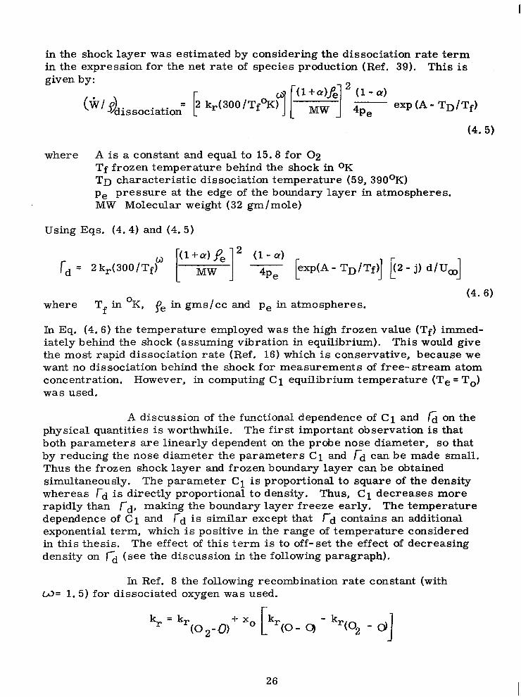
in the shock layer was estimated by considering the dissociation rate term in the expression for the net rate of species production (Ref. 39). This is given by:

( lp) lb dissociation exp (A - TD/Tf)

(4.5)

where A is a constant and equal to 15.8 for 02 Tf frozen temperature behind the shock in oK TD characteristic dissociation temperature (59, 390°K) pe pressure at the edge of the boundary layer in atmospheres. MW Molecular weight (32 gm/mole)

Using Eqs. (4.4) and (4.5)

f-d = 2 kr(300/Tf)ti I’+;?]” 2 kp(A-TD/Tfj C(2-j)d/Um]

(4.6) where Tf in OK, fe in gms/cc and pe in atmospheres.

In Eq. (4.6) the temperature employed was the high frozen value (Tf) immediately behind the shock (assuming vibration in equilibrium). This would give the most rapid dissociation rate (Ref. 16) which is conservative, because we want no dissociation behind the shock for measurements of free- stream atom concentration. However, in computing Cl equilibrium temperature (Te = To) was used.

A discussion of the functional dependence of Cl and fd on the physical quantities is worthwhile. The first important observation is that both parameters are linearly dependent on the probe nose diameter, so that by reducing the nose diameter the parameters Cl and rd can be made small. Thus the frozen shock layer and frozen boundary layer can be obtained simultaneously. The parameter Cl is proportional to square of the density whereas rd is directly proportional to density. Thus, Cl decreases more rapidly than fd, making the boundary layer freeze early. The temperature dependence of Cl and fd is similar except that rd contains an additional exponential term, which is positive in the range of temperature considered in this thesis. The effect of this term is to offset the effect of decreasing density on rd (see the discussion in the following paragraph).

In Ref. 8 the following recombination rate constant (with W= 1.5) for dissociated oxygen was used.

k, = k, (0 2-U)

+ x~ kr (O- (2 - kr(O 2-d

1

26

with

.

%oz - 0) = 1016 cc2/mole2- set

kr(O - 0) = 8.6 x 1016 cc2/mole2-sec.

x0 is the mole fraction of oxygen atoms = 20/( 1 +(Y)

In nonequilibrium nozzle flow calculations described in Sec. 3.3 (Ref. 14) the following recombination rate constant was used.

k,(300 /TfoK,w = 2.86 x 1022(TfoKJ2. l2 cc2 /mole 2 -sec.

The values of Cl and fd calculated at three reservoir conditions using both the preceding values for k, are given in Table 4. 1. This was done to see whether there would be any significant changes in the values of Cl and rd by using different temperature dependence for k,. It is apparent from Table 4.1 that there are no significant differences between the values of Cl corresponding to W= 1.5 and 2.12. However, the values of rd for W = 1.5 . are about twice those for c3 = 2.12. It is interesting to note that, even though the reservoir pressure, and hence reservoir density, increases from 14.4 atmos . to 40. 7 atmos, fd 61 v ues tend todecrease as the reservoir pressure increases. This is due to the fact that the frozen temperatures (Tf) decreases as the dissociation concentration and total enthalpy decrease, making the exponential term in /-d smaller. The increase in reservoir density is offset by the decrease in frozen temperature. The values of Cl given in the Table 4.1 are much less than the required value for frozen boundary layer criteria. The values of l-d (especially for W = 1.5) are slightly more than the required value in a few cases, However, this should not be of any concern, since an order of magnitude has been already added to the limit rd 4 3 x 10W2. Furthermore, by using frozen temperature immediately behind the shock, the most rapid dissociation rate is assumed because the frozen temperature reaches maximum immediately behind the shock. Thus the use of the frozen temperature is again conservative.

4. 3 Selection of Probe Sizes and Configurations

To measure the catalytic efficiency and free-stream atom concentration, either a combination of axisymmetric and two-dimensional probes or two geometrically similar probes can be used (Sec. 2.2). The ratio of diameters is selected by sensitivity considerations. The absolute size of the probe is determined by considerations of fabrication feasibility and by the frozen shock layer and frozen boundary layer criteria. The maximum diameter of the probes cannot be more than 10 mm in order to ensure frozen chemistry around the probe (Sec. 4.2 and Table 4.1). The minimum diameter of the probe (6 mm. dia. ) was dictated by the available size of grinding and polishing tools (see Appendix A). Thus, a combination of 6 mm dia axisymmetric probe and 10 mm dia two-dimensional probe was selected

27

which gave a diameter ratio (dg/d2) of 0.6. This ratio is within the operating regime (Fig. 2. 1). If a combination of two geometrically similar probes were to be used, then the diameter ratio (dg,/dgl) should be at least 0.3 (Fig, 2.2), which gives a combination of 3 mm and 10 mm dia probes. This combination was discarded due to fabrication difficulties.

From the above discussion it is apparent that the range of probe sizes that can be used is rather limited. This is due to low stagnation temperatures and low flow Mach numbers (hence high flow densities) in the test section (see discussion of functional dependence of Cl and fd on flow quantities in Sec. 4.2.2). However, this technique of measuring free-stream atom concentration will be more flexible in advanced hypersonic shock tunnels where the test section Mach numbers of 20 to 30 (hence low flow densities) and the stagnation temperatures of 6000°K to 8000°K are obtained, so that probe diameters as high as a foot could be used (Ref. 16). This technique could also be used to study the non-equilibrium flow phenomena along the nozzle centreline in these advanced facilities.

5. EXPERIMENTS AND RESULTS

5.1 Introductory Remarks

The working principle of a catalytic probe to measure free stream atom concentration (Ref. 16) in low density hypersonic flows is outlined in Chapter 1. A catalytic probe consists of a pair of thin film heat transfer gauges mounted at or near the stagnation region. On top of these films, materials like silicon monoxide, magnesium fluoride or titanium dioxide (5 x lo3 A0 to lo4 A0 thick) are deposited by vacuum evaporation technique. These coatings serve the purpose of electrically insulating the thin-film from ionization effects and slso discourage oxygen atom recombination at the surface of the thin film (efficient non-catalytic surfaces). A thin film of silver, (lo3 A0 to 2 x lo3 A”) deposited (by vacuum evaporation technique) on top of the non-catalytic surface serves as a good agent for oxygen atom recombination (efficient catalytic surface). A pair of such heat transfer gauges, both coated with a non-catalytic material and one of them coated with silver on top of non-catalytic surface, mounted side by side make up a differential heat transfer gauge. These can be mounted either on two- dimensional or on axisymmetric probes.

The experimental program consisted of measuring stagnation point heat transfer in the UTJAS 11 in. x 15 in. hypersonic shock tunnel test section at the reservoir conditions given in Table 3. 1. Thin-film heat transfer gauges fired on .Pyrex backing material were used to measure the surface temperature rise. Pin-hole free, thin-film gauges were made by using Hanovia - 05X platinum paint. The technique of making these gauges and their operating principle are outlined in Appendix A. The thin film gauges were made on Pyrex #7740 as two-dimensional and axisymmetric gauge in-

28

serts (see Fig. A. 1) so that these small inserts could be mounted in the larger metal probes. The details of the fabrication technique of these inserts are also given in Appendix A. The signals from the thin film gauges were amplified before they were applied to the analogue network. The output from the analogue network is directly proportional to the heat transfer rate. The operating principle of the analogue network and its design are outlined in Appendix B (see also Fig. B. 1). The analogue network and the associated amplifier are shown in Fig. B. 2.

5.2 Coating Technique of Heat Transfer Gauges

The thin film heat transfer gauges (500 to 700°A thick) were coated with a lo4 Ao thick silicon monoxide and on top of this a coating of 2000°A thick silver was deposited by vacuum evaporation technique. The details of the vacuum evaporation technique are outlined in Appendix A. Clean- ing the Pyrex surface around the thin film with lens cleaning paper and heating the gauge inserts in air at i’50°F for 5 to 6 hours after the gauge has been coated with the non-catalytic material improved the durability of the silicon monoxide coating*. These gauges were used 10 to 15 times. The resistance of thin films was checked before and after the coating was put on, and any gauge with a slight change in resistance was discarded. Shorting through the silver surface was avoided by masking a small region, where the thin film was joined to the lead wires, with a blob of printing ink**. No change in resistance of thin films was observed during repeated runs.

The effect of discontinuity in the catalytic surfaces on heat transfer has been treated analytically in Ref. 40. If the heat transfer gauges are coated with silver in such a way as to cover only a small portion of the surface of the gauge, the measured heat transfer could be affected by recombination of the atoms crowded at the edge of the catalytic surface. However, this edge effect diminishes very quickly away from the edge, so that the edge effect becomes negligible if the catalytic surface plan form area is much larger than the thin-film area. In the present experiments the axisymmetric probes were coated with silver throughout the spherical surface. In the case of two-dimensional probes, the area of the silver surface compared to the thin film area was large enough not to cause any edge effect on the measured heat transfer.

The response time of thin film gauges (500°A to 750°A thick) is in the order of a few psecs. Due to the thick coatings on top of thin film

* Gauges coated with a thickness of 60000A, without any treatment either before or after the coating, were very unsuccessful. Apparently the coating peeled off when the gauge was used a couple of times. Difficulties in making a good non-catalytic gauge were also experienced by other research workers (Ref. 8). A 2000°A thick il s ver coating was used throughout this work, since this thickness was sufficient to withstand repeated runs.

** The printing ink was made by “Sinclair and Valentine Company of Canada and of type Gloss Black N- 18 1”.

29

the response time should not affect the heat transfer measurements in shock tunnels since the testing time will be in the order of milliseconds.

It is desirable to consider the assumption that the surface temperature sensed by the thin-film is the actual surface temperature (see Appendix A). The validity of this assumption depends on the time interval of interest (i. e., time (PC 12/k).

available testing time) and the characteristic heat diffusion If the time interval is large in comparison with this character-

istic time the preceding assumption is satisfactorily accurate (Ref. 41). The effect of thickness of thin-film on surface temperature has been studied in detail in Ref. 41. It was found that the error in surface temperature measurement will be reduced to about 2% after a time elapse of 100 wsec with a one micron thick platinum film. In the present case the platinum film thickness was 500 to 7OOOA so thattheerror due to platinum film is negligible. However, a lo4 OA (1 micron) thick silicon monoxide was used on top of platinum film. Considering the effect of this coating on the measured surface temperature, the value of heat diffusion time is 1.78 x low7 set for a one micron thick coating. This value is approximately 4 times more than the value for the platinum film of the same thickness (4.2 x 10m8 sec. ). But in the present work the heat transfers were measured after a time lapse of nearly one millisecond (see Sec. 5.6), so that the time interval is 5600 times longer than the heat diffusion time. Thus, the error in the measured heat transfers due to this effect is negligible. In the case of catalytic gauges an additional coating of silver (2OOOOA thick) should not affect the measured heat transfers since silver is a very good conductor (heat diffusion time is very short) and also the thickness of the film is small.

5. 3 Arrangement of Catalytic Probes

A combination of two-dimensional and axisymmetric catalytic probes was used to measure the differential heat transfers. The two-dimensional probe was in the form of a blunted wedge with a nose diameter of 10 mm and 9 in. long and the axisymmetric probe was in the form of a blunted cone with a nose diameter of 6 mm. This combination gave a diameter ratio (d3/d2) of 0.6. The reasons for selecting these sizes are given in Sec. 4.3. Two heat transfer gauge inserts (one catalytic and the other non-catalytic) were mounted a few mm apart along the stagnation line of the two-dimensional probe (Fig. 5. 1). In the case of the sxisymmetric probe, an attempt was made to make the two thin-film gauges near the stagnation region in the form of a V-shape (similar to the one described in Ref. 8). However, the two thin- film gauges could not be fired near the stagnation region due to the small diameter (6 mm. ) of the probe. Therefore, it was decided to make only one thin- film gauge on the axisymmetric probe as shown in Fig. A. 1 and use two separate probes mounted side by side (as shown in Fig. 5. 1) to measure the differential heat transfer to the axisymmetric probe. Due to the lack of flow uniformity along the vertical centreline (15 in. plane) as shown in Fig. 3.8, all the probes were mounted along the horizontal centreline (11 in. plane). Along this centreline, only two probes were mounted in a given run (each probe 0.75 in. from centreline) in order to avoid the effects of slight flow asymmetry in

30

this plane (see Fig. 3.7 ). This necessitated the use of two repeated runs to obtain the differential heat-transfers to both the two-dimensional and axisymmetric probes. In one run two axisymmetric probes mounted l- l/2 in. apart as shown on the top half of the Fig. 5.1 were used and in the repeated run the two-dimensional probe and one of the axisymmetric probe were used as shown in the bottom half of the Fig. 5.1. The repeatability of runs was good in the sense that the incident shock Mach numbers were measured within a variation of 2 2% and the reservoir pressures were measured within 2 50/O, (see Table 5.1). These percentages are within the accuracy of the measurements.

5. 4 Effect of Rdiation on Measured Heat Transfers

The effect of radiation from excited oxygen atoms and molecules, if any, on heat transfer measurements was found to be negligible. This was established by conducting the following qualitative test. Aluminum has been shown to be very non-catalytic (Ref. ll), but it should respond like silver to radiation. Thus, if the heat transfers to silicon monoxide and aluminium coated gauges are measured, then the difference between these two measured values should be due to radiative heat transfer, because the coefficients of obsorption of silicon monoxide and aluminium are not equal. It can therefore be concluded that the role of radiative heat transfer is negligible, if the two heat transfers are equal. A few heat transfer gauges were coated with aluminum instead of silver coating. The heat transfers to silicon monoxide and aluminum coated gauges were measured and the outputs from the analogue network are shown in Fig. 5.2(a). No measurable differential heat transfers could be obtained from these records, establish- ing the negligible role of radiation on the measured heat transfers.

The following test was also done to check the uniformity of the flow and the identical behavior of the different pre-amplifier channels and analogue networks. The amplification factor for all channels was set at 56 using a sine wave generator. Two uncoated gauges having nearly equal gauge properties ( qs and cuf) were installed in the probes and the probes were mounted in the test section. The initial voltage (ugo) across the gauges were all set equal to 0. 5 Volt using a Keithely digital voltmeter. Thus, the outputs from the analogue network should be equal (see Eq. B. 1) if the flow is uniform. The difference signal from these two gauges was monitored using a differential plug-in unit. As expected no measurable difference in the signals was found as shown in the Fig. 5. 2(b).

5.5 Experimental Procedure

The differential heat transfers to the two-dimensional and axisymmetric probes were measured by using the following procedure. The probes were mounted in the 11 in. x 15 in. nozzle station and l-1/2 in. apart along the horizontal centreline (11 in. plane). Then the test section, the dump tanks and the channel were evacuated using the pumping system described in Sec. 3.1, until the pressure reached about 5 FHHg in the test section and about

31

50 FHg in the channel. The heat transfer gauges were connected to the analogue network through a pre-amplifier (see Fig. A. 1). The initial voltage across all the gauges were set at 0.5 Volt. Since the built-in voltmeter in the anslogue network was not accurate enough a Keithely digital voltmeter was used to measure the initial voltage across the gauges. The amplification factor for all the four channels was set at 56. The outputs from the anslogue were measured using a dual beam oscilloscope (Tektronix 565 with 3A3 plug-in units). The built-in filter in 3A3 plug-in unit was used in all the runs to cut off the high frequency noise. The source of this noise is believed to be due to slight nonuniformity in the flow which will be amplified in the snalogue network because, the signal is essentially differentiated at the snalogue output. The channel was flushed with the test gas (oxygen*) a few times and evacuated before the channel was chared up to the required pressure. Then the driver was charged with a stoichiometric mixture of oxygen and hydrogen diluted with 70% Helium, and 8 to 10 minutes were allowed for the gas to mix properly before the tube was fired. In all the runs, shock speed, reservoir pressure and outputs from the analogue network were recorded. These measurements were repeated a number of times at every reservoir condition given in Table 3. 1. Typical heat transfer and reservoir pressure traces recorded at a reservoir pressure and temperature of 22.2 atmos., and 4700°K respectively, are shown in Fig. 5. 3. In all the four heat transfer traces there is an initial unsteady portion (a to b in Fig. 5. 3) due to starting process in the nozzle system. This is followed by a steady portion (b to c in Fig. 5.3) which corresponds to the testing time. The steady heat transfer tends to fall-off in a similar manner to the reservoir pressure history shown in Fig. 5.3. This is due to the effect of reflected rarefaction wave in the shock tube. The initial unsteady portion in the heat transfer histories is slightly different for axisymmetric and two-dimensional probes. This may be due to the different type of flow establishment around the probes. The slight bump in the reseroir pressure history is believed to be due to nonuniform combustion in the driver. Note that, this bump is faith- fully reproduced in the two-dimensiondl heat transfer histories. However, in the axisymmetric case it does not appear because it did not appear in the reservoir pressure history.

Before the actual measurements were recorded, the gauges were exposed to the oxygen atoms by running the shock tunnel a few times to convert the pure silver into silver oxide. This was necessary because, the silver oxide and not the virgin silver is responsible for surface recombination of oxygen atoms (Ref. 42). This aspect is discussed in Chapter 6.

* Bottled oxygen supplied by “CANOX” Canadian Oxygen Limited was used as the test gas. The quoted purity level of oxygen is 99.9%. The impurities are Argon and water vapour.

32

5. 6 Reduction of Data

From the analogue outputs (Fig. 5.3) it may be noted that about 500 to 700 @set of testing time are taken up by the starting process in the nozzle system. Afterwards the heat transfer traces remain constant for about a millisec, before the effect of the reflected rarefaction wave in the shock tube is felt (note also the similar reservoir pressure history shown in Fig. 5. 3). At all the reservoir conditions investigated, the duration of testing time computed from consideration of arrival of reflected rarefaction wave in the shock tube was shorter than the time required to consume the slug of test gas. In reading off the ordinate from the heat transfer traces, the steady portion (w. r. t. time) was always used. The heat transfer rates were computed using Eq. B. 1 and the gauge constants obtained by the calibration technique outlined in Appendix C.

The heat transfers to the axisymmetric probes were corrected because the thin film gauge had a finite length wrapped around the stagnation point, so that the measured heat transfer was an average value rather than the value at the stagnation point. This correction was made using the theoretical heat transfer distribution around an axisymmetric body (Ref. 1). The correction was about 8%. This type of correction was not needed in the case of heat transfers to the two-dimensional probe since the thin film gauge was constructed along the stagnation line.

If the surface temperature rise is fairly high, then the properties of the substrate material (Pyrex), ks, ps and cs will change so that the measured heat transfers obtained by using the value of (k p c)~ at room temperature will be in error. A thorough discussion of this problem with a simple method of correcting for this effect is given in Ref. 43. However, this type of correction was negligible for the rate of heat transfers reported in this thesis.

The computed heat transfers along with the measured shock Mach numbers and reservoir pressures of several repeated runs at the same reservoir condition are given in Table 5.1. This table will be used to demonstrate the method of calculating the catalytic efficiency.

5.7 Estimation of gc and cyoo

The probe Reynolds numbers (Rep), based on flow conditions behind the bow shock, varied from 98 to 202 for the 10 mm dia probe and 59 to 122 for 6 mm dia probe. Since these ranges lie in the merged layer regime (Fig. 2. 3), Eq. (2.46) was used to calculate the catalytic efficiency. The ratio of differential heat transfers (632) could be obtained by using any one of the runs in Table 5. l(a) with any one of the runs in Table 5. l(b). Thus, the catalytic efficiency(gc3) was calculated using 12 different combinations and these values are given in Table 5. l(c). The mean of all these values is 0.81

and the standard deviation (6) is 0.048 (6% of mean value). Then gc2 is calculated using the relation between gc3 and oc2 (Eqs. 2.42 and 2.45) and a value of 0.89 is obtained. The slight change in the catalytic efficiency due to the free-stream density and velocity change (see Eq. 1.5) caused by different reservoir conditions is negligible.

In order to calculate ao-,, the Lewis number of oxygen has to be known. This was computed by using the explicit formulae given in Ref. 44 for binary diffusion coefficient (D12) viscosity ( p) and coefficient of heat conductivity (k) as functions of temperature. The collision cross section (612) for a mixture of oxygen atoms and molecules was taken as an average value of the collision cross sections for atoms and molecules. Then, using the value of QIc3 or 0 c2 (as the case may be) the free-stream atom concentration was computed from Eq. (2. 11) or (2. 12). It is interesting to note that the differential heat transfer, either from the axisymmetric or from two-dimensional probe, is sufficient to obtain (Y oo, provided the proper value of catalytic efficiency (cbc3 or gc2) is used.

The mean values of ao., obtained at five reservoir conditions and the standard deviations (obtained by repeated runs) are given in Table 5.2. The computed values of (Ye using the non-equilibrium nozzle flow analysis (Sec. 3. 3) are also given in Table 5.2. These results are discussed in the next Chapter.

Free-stream atom concentrations were also measured at 6 in. upstream from the 11. x 15 in. station. This was done with a view to check whether the flow was frozen along the nozzle centre line since frozen flow in the terminal nozzle was predicted by the nonequilibrium nozzle flow calculations of Ref. 14. No measurements were done beyond this station because of the probe mounting difficulties and because frozen shock layer criteria may be violated due to higher free stream densities in the nozzle. am values measured at this station for three reservoir conditions are given in Table 5. 3. These results are discussed in the next Chapter.

6. DISCUSSION OF RESULTS AND CONCLUSIONS

The measured values of catalytic efficiencies for axisymmetric and two-dimensional probes are given in the Table 5. 1. No attempt has been made to compute the value of rate of recombination (k,) at the silver surface, since the diffusion velocity(S3 or S2) is not known. Because the density and the viscosity of the gas behind the bow shock and the free- stream vd ocity in the test section are not known accurately. However, the estimation of kw is not necessary for computing the value of CY~. Conversely, if kw is directly measured from glow discharges experiments (Ref. 8 and ll), then the flow quantities in any given experimental condition have to be known accurately to estimate 0,. 2000 cm/ sec.

In Ref. 8, oc values have been estimated using a value of kv, = A direct comparison of dc values with the present values is not

possible due to the different experimental conditions. However, since these values are not very much different from the present values of gc, it may be concluded that silver surfaces seem to behave in the same manner as they would behave in glow discharge experiments (at least with respect to the value of catalytic efficiency).

The ratios of measured heat transfers, (qc3/qc2) and (9nc3/qnc2), were calculated by using the mean values obtained from the repeated runs given in the Table 5.1. theoretical ratios could easil be obtained since (qnc3/qnc2) = (2d2/d3) Correspond~~2 and (qc3/qc2) ;J (2d2/d3)‘/2$: These relations can easily be derived from Eq. (1. 6). The theoretical ratios are compared with the measured ratios in the Table 5.1. The agreement is good in the sense that the error between the theory and experiment is within 5%.

The measured values of Q~ at 11 in. x 15 in. station in the nozzle are compared with the theoretical values computed from nonequilibrium nozzle flow calculations (Sec. 3. 3) in Table 5. 2. The standard deviation from the mean value of ao-, due to repeated runs is also given. The percentage difference between the computed values and the measured (mean) values is given in the last column.

Before a direct comparison can be made between the theory and experiment, the accuracy of the computed values has to be determined. This is done by the following procedure. The theoretical model used for nonequilibrium nozzle flow calcuations (Sec. 3.3) is assumed to be a good representation of the non-equilibrium flow phenomenon in the nozzle because hitherto neglected effects such as coupling between vibration end dissociation, effect of preferential dissociation from higher vibrational levels, are taken into account. Since the mass fraction froze very early in the primary nozzle, the boundary layer along the nozzle walls should not affect the computed ao, values. The other source of error involved in these computations is the effect of inaccuracies in the input quantities; namely, reservoir pressure (PO) and temperature (To). The method of determining PO and To in any given running condition is outlined in Sec. 3. 2. The reservoir pressure (which is used in the nozzle flow calculations) could be measured to within f 5% by using Kistler 605 pressure transducers (see Sec. 3. 2). The stagnation temperature is taken from shock tube tables corresponding to the measured shock Mach number which was measured with an accuracy of f 2%. However, this temperature was corrected for the effect of shock wave-boundary layer interaction in the shock tube by a method outlined in Sec. 3. 2. The accuracy of this method is questionable and more will be said about this effect later. Therefore, the stagnation temperature was taken as f 2% accurate. This is based on the fact that the shock Mach number was measured with an accuracy of 2 2% and for a two percent change in MS the error in To, which is approximately f 2% for the range of shock Mach numbers considered, was obtained from shock tube performance tables (Ref. 28). These errors in PO and To were used in the computer programme and the corresponding a00 values were also computed. These values are shown in Table 5.2 as a fraction of the nominal value. It is interesting to note that, for a * 5% change in PO and a * 2% change in To (at all the

35

reservoir conditions), the error in the computed values of CQ, varies between f8qo to f 11%. Furthermore, an error of 23% in To with the same 25% error in PO causes an error of 213% to 216% in the values of aao. Thus the values of ace is very sensitive to changes in To.

The absolute. accuracy with which (L& and cr, can be measured, using the present self-calibrating technique, was determined by an error analysis. The details of the error analysis are outlined in Appendix D. This analysis showed that ao, can be measured with an accuracy of ?S. 0%. The error between the computed vslues and the measured (mean) values is given in the last column of Table 5.2. If one considers the accuracy with which the values of CYa can be computed (as described above), the differences between the computed and measured values are not unreasonable. Also, the error tends to decrease monotonically in the case of first three reservoir conditions as the reservoir pressure increases. A possible explanation would be that the boundary layer interaction effect on To might be more severe at low reservoir conditions causing more error in the predicted value of To. This might also be entirely coincidental.

It has been noticed (Ref. 36) that the vibrational relaxation time for nitrogen in expansion flows (nozzle flows) is much faster (10 to 20 times) than that measured behind normal shocks. It was therefore decided to have Ref. 14 also use much faster vibrational relaxation times in the non-equilibrium nozzle flow calculations for oxygen and to calculate (Ye. If considerable differences in Q, vslues are obtained, then by comparing these values, some- thing can be said about the vibrational relaxation times in expansion flows for oxygen. The Q, values computed using vibrational relaxation times equal to and one twentieth of the value behind normal shocks (V = 1.0 and 0.05) are given in the Table 5. 2. The difference between the values corresponding to t.’ = 1.0 and 0.05 is a maximum at the low reservoir pressure (8.5%) and this difference reduces to 2.6% at the high pressure reservoir condition. If the errors in the computed values are reduced by an accurate determination of the reservoir conditions, then a comparison between these values (for t’ = 1.0 and t’ = 0.05) and the measured values could lead to some conclusions about the . vibrational relaxation times, at least at the low reservoir pressure levels where the difference between (rco (t’ = 1.0) and ao-,(t = 0.05) is a maximum. However, from the present measurements no definite conclusions can be drawn because the differences between the computed and measured values might be due to errors in the reservoir temperature and pressure. Nevertheless, the results do favour the low value of tV .

The LQ, values measured at 6in. upstream of 11 in. x 15 in. stationare given in Table 5.3. The percentage difference between the theory and measured values is shown in the last column. This error seems to have the same sign and approximately the same magnitude as that given in the Table 5.2 in the case of the first two reservoir conditions, whereas in the last case the error seems to increase by about 10% (probe is measuring more than the predicted value). It should be noted that the same reservoir conditions

36

were used and the theoretical values of cro-, are the same as those given in Table 5.2, since the flow was frozen throughout the terminal nozzle (Sec. 3.3). Then, the above discrepancy might be explained by further dissociation in the shock layer due to increased density at this station.

It has been established in Ref. 42 that pure silver is essentially non-catalytic and silver oxide formed on the silver surface is reponsible for high catalytic activity of the silver surface. A tenative mechanism for oxygen atom recombination on the surface might require a molecule such as silver oxide (Ag20) to pick up an oxygen atom and form argentic oxide (Ago),

Ag20+ 0 --t2 Ag 0 (5.1)

this is called the capture reaction.

Subsequently argentic oxide picks up another oxygen atom and forms silver

2 AgO+ 0 -7Ag20+02 (5.2)

This is called the release reaction.

The contribution to the measured heat transfer due to oxide formation is negligible. This is demonstrated in Ref. 9 by a quantitative example. Considering the case of three layers of Ag20 being formed, the heat transfer due to Ag20 formation is 5. 5 x 10m3 BTU/ft2- set, which is negligible compared to the measured heat transfer rates.

Some peculiarities were observed in the behaviour of a silver surface when it was used in a shock tube flow. For example, the stagnation point heat transfer increased with time (Ref. 8) instead of remaining constant with time. This effect was thought to be perhaps due to slow surface reaction rate (Ref. 12). This possibility could be ascribed to submechanisms in the phenomenon of surface atom recombination. For example, an atom must be adsorbed on to a surface, it must diffuse to an active site where it combines with another atom, and then the molecule desorbs. If the time scale for all these events to occur is of the same order as the delivery rate of atoms in an experiment, it is conceivable that the observed time dependence of stagnation point heat transfer measurements could be reconciled. Thompson et al (Ref. 12) used a glow discharge shock tube (GDST) facility to further investigate this phenomenon. Briefly, the GDST combines the ordinary glow discharge tube and the shock tube. First, they measured the differential heat transfers by using only the glow discharge tube in which case the rate of atoms delivered to the catalytic surface is relatively low. Then the flow of atoms were accelerated by using the facility as a GDST. By this process the same atoms were delivered to the surface at a rate three orders of magnitude faster than before. The measured differential heat transfers in this were compared with the previous measurements and they found no change with respect to time in either case. Thus, they concluded that the surface reactions are rapid enough

37

to follow the sudden changes in atom flux, and the time dependence of differential heat transfers observed in the shock tube experiments was perhaps due to slow dissociation relaxation in the shock layer. However, there was still some doubt as to the behavior of a catalytic gauge when it is used in hypersonic free stream to measure atom concentration. During the present heat transfer measurements, the records were closely observed and there was no time dependence of stagnation point heat transfer rates. This confirms, that the surface reactions are fast enough to follow the sudden changes in atom flux and cause no time dependent characteristics. Thus, the catalytic gauges could be used with confidence to measure free stream atom concentrations.

Based on experimental results and the preceding discussions concerning data, the following conclusions are stated:

1) The feasibility of measuring the catalytic efficiency with the gauge exposed to the actual flow conditions was demonstrated by measuring catalytic efficiency in the UTLAS 11 in. x 15 in. Hypersonic Shock Tunnel test section.

2) The atom concentrations in a hypersonic free stream were successfully measured by using the self-calibrating technique in which a pre- knowledge of the catalytic efficiency is not necessary and the requirement of knowing the flow quantities, except the stagnation enthalpy and the Lewis number, to measure the free Etream atom concentration is eliminated.

3) The absence of any time dependent character of catalytic surface reactions was confirmed (see discussion).

4) With this method the catalytic efficiency and the free stream atom concentration could be measured with an accuracy of 2 4% and f .6% respectively (see Appendix D).

5) The nonequilibrium flow analysis of Tirumalesa (Ref. 14) used in this report to compute the atom concentration along the nozzle centre line, is believed to be a good representation of the flow phenomenon. But unfortunately the computed value of ao, is very sensitive to the errors in the reservoir conditions (see discussion). Unless the reservoir temperature is either computed or measured quite accurately a meaningful comparison is difficult. Although the procedure might be reversed to infer reservoir temperature from the measured value of aoD and the nonequilibrium nozzle flow calculations, it would be necessary to test the accuracy of the present method of measuring (Y~ by an independent technique (such as an electron gun), in order to obtain substantiating data.

38

REFERENCES

1. Lees, L.

2. Fay, J. A. Riddell, F. R.

3. Goulard, R. J.

4. Cheng, H. K.

5. Chung, P. M. Liu, S. W.

6. Inger, G. R.

7. Buckmaster J. K.

8. Hartunian, R. A. Thompson, W. P.

9. Myerson, A. L.

10. Myerson, A. L.

Laminar Heat Transfer Over Blunt-Nosed Bodies at Hypersonic Flight Speeds, Jet Propulsion, Vol. 26, No. 4, April, 1956. ,pp. 259-269.

Theory of Stagnation Point Heat Transfer in Dissociated Air, Journal of the Aeronautical Sciences, Vol. 25, No. 2, Feb. 1958,~~. 73-85, 121.

On Catalytic Recombination Rates in Hypersonic Stagnation Heat Transfer. Jet Propulsion, Vol. 28, No. 11,Nov. 1958,~~. 737-745.

Hypersonic Shock Layer Theory of the Stagnation Region at Low Reynolds Number. Proceedings of the 1961 Heat Transfer and Fluid Mechanics Institute (Stanford University Press, Stanford, Calif. 1961,p. 161.

An Approximate Analysis of Simultaneous Gas- Phase and Surface Atom Recombination for Stagnation Boundary Layer. Aerospace Corp. Report No. TDR-169, (3230-12) TN-4, Nov. 1962.

Nonequilibrium-Dissociated Stagnation Point Boundary Layers with Arbitrary Surface Catalyticity. AIAA Journal, Vol. 1, No. 8, August 1963, pp. 1776 - 1784

The Effects of Ambient Dissociation on Frozen Hypersonic Stagnation Flow. AEDC-TDR-64- 142, June 1964.

Nonequilibrium Stagnation Point Heat Transfer Including Surface Catalysis. AIAA Paper No. 63- 464. AIAA Conference on physics of Entry into Planetary Atmospheres, M. I. T. August 1963.

Silver-Catalyzed Recombination in a Step- Function Flow of Atomic Oxygen. The Journal of Chemical Physics, Vol. 38, No. 8 2043-2045, 15 April, 1963.

Mechanisms of Surface Recombination from Step-Function Flows of Atomic Oxygen over Noble Metals. The Journal of Chemical Physics, Vol. 42, No. 9, 3270-3276, 1 May, 1965

39

11. Hartunian, R. A. Thompson, W. P. Safron, S.

12. Thompson, W. P. Hartunian, R. A.

13. Carden, W.H.

14. Tirumalesa, D.

15. Rosner, D. E.

16. Hartunian, R.A.

17. Lewis, B.

18. Linnett, J. W Marsden, D. G. H.

19. Li, T.Y. Griger, R. E.

20. Myerson, A.L.

21. Hartunian, R. A. Liu, S. W.

Measurements of Catalytic Efficiency of Silver for Oxygen Atoms and the O-02 Diffusion Coefficient, The Journal of Chemical Physics, Vol. 43, No. 11, pp. 4003-4006, 1 Dec. 1965.

Catalytic Probe Response to High Atom Flux in a Glow Discharge Shock Tube, AIAA Journal, Vol. 3, No. 4, 790-791, April, 1965.

Experimental Heat Transfer to Hemispheres in Nonequilibrium Dissociated Hypersonic Flow with Surface Catalysis and Second-Order Effects, AEDC-TR-65-127, July 1965.

Nozzle Flows with Coupled Vibrational and Dissociational Nonequilibrium, UTLAS Report (to be published)

Catalytic Probes for the Determination of Atom Concentrations in High Speed Gas Streams, ARS Journal, Vol. 32, No. 7,pp. 1065-1073. July, 1962.

Local Atom Concentrations in Hypersonic Dissociated Flows at Low Densities, Physics of Fluids, Vol. 6, No. 3,pp. 343-348, March 1963.

Combustion Processes, Vol. II of the High Speed Aerodynamics and Jet Propulsion, Princeton University Press, 1956.

The Kinetics of the Recombination of Oxygen Atoms at a Glass Surface and The Recombination of Oxygen Atoms at Salt and Oxide Surfaces, Proc. of the Royal Society, Series A, Vol. 234. March 1956, pp. 489-515.

Stagnation Point of a Blunt Body in Hypersonic Flow. J. Aero. Sci. , Vol. 24, pp. 25-32, (1957)

Interim Report on Transient Heat-Transfer Measurements of Catalytic Recombination in a Step-Function Flow of Atomic Oxygen, CAL. Report AF-1412-A-2 (1962).

Slow Flow of a Dissociated Gas About a Catalytic Probe. The Physics of Fluids, Vol. 6, No. 3, March, 1963.

40

22. Hartunian, R.A. Marrone, P. V.

23. Rosner, D. E.

24. Vidal, R. J. Wittliff, C. E.

25. Chan, Y.Y. Mason, R. P. Reddy, N. M.

26. Mason, R.P. Reddy, N. M.

27. Flagg, R. F.

28. Bernstein, L.

29. Mark, H.

30. Rudinger, G.

31. Woods, B. A.

32. Glass, I. I. Tokano, A.

Heat Transfer from Dissociated Gases in a Shock Tube, CAL Report AD-1118-A-7, (1959)

Similitude Treatment of Hypersonic Stagnation Heat Transfer* ARS Journal, Vol. 29, No. 3, March, 1959, pp. 2 15-2 16.

Hypersonic Low-Density Studies of Blunt and Slender Bodies, Paper presented at the Third International Symposium on Rarefied Gas Dynamics, Paris, France, June 26-29, 1962.

Instrumentation and Calibration of UTIAS 11 in. x 15 in. Hypersonic Shock Tunnel, TN 91, June 1965.

Combustion Studies in the UTIAS Hypersonic Shock Tunnel Driver, 5th Shock Tube Symposium, U. S. Naval Ordnance Laboratory (April 1965).

Detailed Analysis of Tailoring Conditions in a Combustion-Driven Shock Tunnel, AVCO. Tech. Memo. RAD-TM-63-12, March, 1963.

Tabulated Solutions of the Equilibrium Gas Properties Behind the Incident and Reflected Normal-Shock Wave in a Shock Tube, 1. Nitrogen. 2. Oxygen. , ARC-CP-626, 1963.

The Interaction of a Reflected Shock Wave with The Boundary Layer in a Shock Tube, NASA TM 1418, March 1958.

The Effect of Boundary Layer Growth in a Shock Tube on Reflection From a Closed End, Physics of Fluids, Vol. 4, No. 12, 1961.

A Linearized Investigation of the Effect of a Wall Boundary Layer on the Motion of a Reflected Shock,. RAE Tech. Note Aero 2848, Oct. 1962.

Nonequilibrium Expansion Flows of Dissociated Oxygen Around a Corner, UTIA Report No. 91, June, 1963, University of Toronto, Institute for Aerospace Studies, Toronto, Canada.

41

33. Glass, I. I.

34. Der, J. J.

35. Emanuel, G. Vincenti, W. G.

36. Hurle, I.R. Russo, A. L. Hall, J. G.

37. Hertzberg, A.

38. Chung, P. M.

39. Inger, G. R.

40. Chung, P.M. Liu S.W. Mirels, H.

41. Vidal, R. J.

42. Myerson, A. L.

43. Walenta, Z. A.

Hyperveloc,ity Launchers, Part 2 : Compound Launchers-Driving Techniques, UTIAS Review No. 26, Dec. 1965. University of Toronto, Institute for Aerospace Studies, Toronto, Canada.

Theoritical Studies of Supersonic Two- dimensional and Axisymmetric Nonequilibrium Flows, NASA, TRR-164, 1963.

Method for the Calculation of the One-dimensional Nonequilibrium Flow of a Gas Mixture through A Hypersonic Nozzle, AEDC-TDR-62-131, June 1962.

Experimental Studies of Vibrational and Dissociative Nonequilibrium in Expanded Flows. Paper Presented at AIAA Conference on Physics of Entry in to Planetary Atmospheres, held at Boston, Aug., 1963.

Private Communication.

Hypersonic Viscous Shock Layer of Non- equilibrium Dissociating Gas, NASA TR-R 109, 196 1.

Nonequilibrium-Dissocated Boundary Layers, with a Reacting Inviscid Flow, AIAA Journal, Vol. 1, No. 9, Sept. 1963.

Effect of Discontinuity of Surface Catalyticity on Boundary Layer Flow of Dissociated Gas, Aerospace Report TDR-69 (2240-20)-TN-l, June 1962.

Model Instrument Techniques for Heat Transfer and Force Measurements in a Hypervelocity Shock Tunnel, Cornell Aeronautical Laboratory, Report No. AD-917-A-1, Feb. 1956.

Silver -Catalyzed Surface Recombination in a Step-Function Flow of Atomic Oxygen, The Journal of Chemical Physics, Vol. 38, No. 8, 2043-2045, 15 April, 1963.

Analogue Networks for High Heat-Transfer Rate Measurene nts, UTIAS TN 84, Nov. 1964.

42

44. Scala, S. M. Baulknight, C. W.

Transport and Thermodynamic Properties in a Hypersonic Laminar Boundary Layer. Part I Properties of the Pure Species, ARS Journal, Vol. 29, No. 11, Jan. 1959

45. Skinner, G. T. Analogue Network to Convert Surface Temperature to Heat Flux, Cornell Aeronautical Laboratory, Report No. 100, Feb. 1960.

46. Meyer, R. F.

47. Taylor, B. W.

48. Skinner, G.T.

49. Beers, Y.

A Heat-Flux-Meter for Use with Thin-Film Surface Thermometer, NRC Aero. Report LR-279, April 1960.

Development of a Thin Film Heat Transfer Gauge for Shock Tube Flows, UTIA TN 27, June 1959.

A New Method of Calibrating Thin Film Gauge Backing Materials, Cornell Aeronautical Laboratory Inc., Report No. CAL-105, June 1962.

Introduction to the Theory of Error, Addison- Wesley Publishing Company, Inc. , Cambridge, Mass, 1953.

43

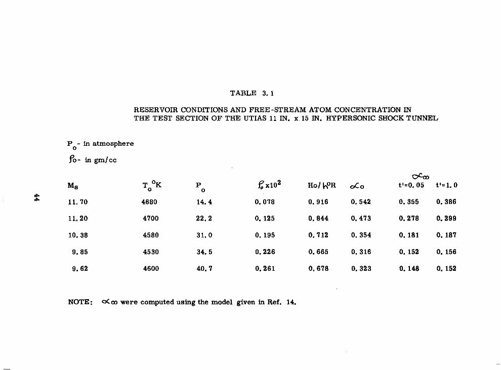
TABLE 3.1

RESERVOIR CONDITIONS AND FREE-STREAM ATOM CONCENTRATION IN THE TEST SECTION OF THE UTIAS 11 IN. x. 15 IN. HYPERSONIC SHOCK TUNNEL

pO- in atmosphere

P o- in gm/cc

MS TooK P 0

& xl02

11.70 4680 14.4 0.078

11.20 4700 22.2 0.125

10. 38 4580 31. 0 0.195

9. a5 4530 34. 5 0.226

9. 62 4600 40. 7 0.261

NOTE : o(oc were computed using the model given in Ref. 14.

Ho/ h”R OCO

0.916 0.542

0. a44 0.473

0. 712 0.354

0.665 0.316

0.678 0.323

occo

t’=O. 05 t’= 1. 0

0.355 0.386

0.278 0.299

0.181 0. la7

0. 152 0. 156

0. 148 0. 152

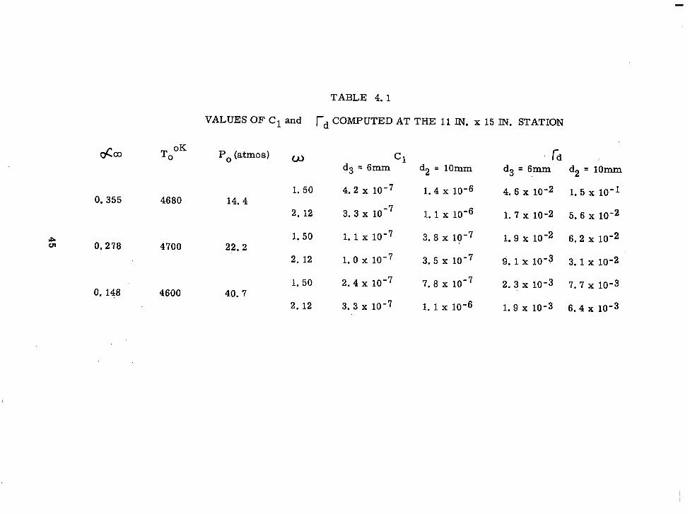
TABLE 4.1

VALUES OF Cl and rd COMPUTED AT THE 11 IN. x 15 IN. STATION

&m TooK

0.355 4680

PO (atmos) u

1. 50 14. 4

2. 12

Cl Td d3 = 6mm d2 = 1Omm d3 = 6mm d2 = 1omm

4.2 x 10-7 1.4 x 10-6 4.6 x 10-2 1.5 x 10-l

3.3 x 1o-7 1. 1 x 10-6 1.7 x 10-2 5.6 x 1O-2

b& 1. 50 1. 1 x 10-7 3. a x 10-7 1.9 x 10’2 0.278

6.2 x 1O-2 ul 4700 22.2

2. 12 1.0 x 10-7 3.5 x 10-7 9.1 x 10’3 3.1 x 10-2

1. 50 2.4 x 10-7 7.8 x 1O-7 2.3 x 10-3 0.

7.7 x 10-3 148 4600 40. 7

2. 12 3. 3 x 10-7 1. 1 x 10-6 1.9 x 10-3 6.4 x 10-3

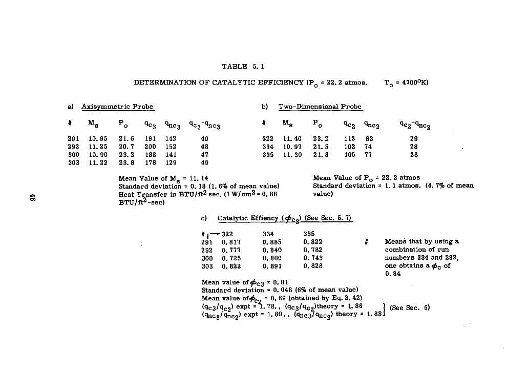
TABLE 5.1

DETERMINATION OF CATALYTIC EFFICIENCY (PO = 22.2 atmos.

a) Axisymmetric Probe b) Two-Dimensional Probe

# % PO qc3 qnc3 %3-%x3 # MS PO qc2 qnc2

291 10.95 21. 6 191 142 49 322 11.40 23. 2 112 83 292 11.25 20.7 200 152 48 334 10.97 21. 5 102 74 300 13.90 23. 2 188 141 47 335 11.30 21.8 105 77 303 11.22 23. 8 178 129 49

TO = 4700°K)

qc2-qnc2

29 26 28

Mean Value of MS = 11. 14 Standard deviation = 0. 18 (1.6% of mean value) Heat Transfer in BTU/ft2 sec. (1 W/cm2 = 0.88 BTU/ft2 -set)

Mean Value of PO = 22.3 atmos Standard deviation = 1. 1 atmos. (4.7% of mean value)

c) Catalytic Effiency (&,,I (See Sec. 5. 7) ”

#i-322 334 335 291 0.817 0.885 0. a22 # Means that by using a 292 0.777 0.840 0.782 combination of run 300 0.725 0.800 0.743 numbers 334 and 292, 303 0.822 0.891 0.828 one obtains a & of

0.84 Mean value of &3 = 0.8 1 Standard deviation = 0. 048 (6% of mean value) Mean value of&

3 = 0.89 (obtained by Eq. 2.42)

(qc3/qc2) expt = .78., (qc3/qc2)theory = 1.86 (~C~/~CSJ) thory = 1.88 1

(See Sec. 6) (9nc31qnc2 ) expt = 1.80.,

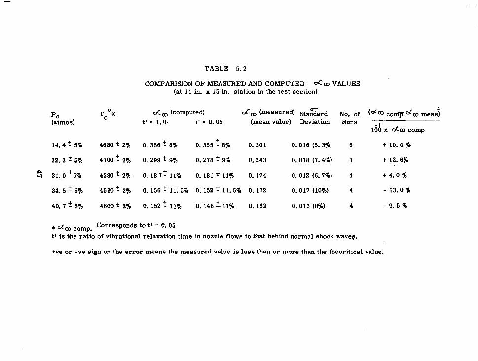
TABLE 5.2

COMPARISION OF MEASURED AND COMPUTED 4 co VALUES (at 11 in. x 15 in. station in the test section)

PO (atmos)

14.4 f 5%

22.2 f 5%

TooK o&-, (computed) da (measured) S&&ard No. of (Occo comxdco meas? t’ = 1.0. t’ = 0.05 (mean value) Deviation Runs

10 3 x Oca, camp

4680 f 2% 0. 386 + 8% 0. 355 + 8% 0.301 0.016 (5. 3%) 6 + 15.4 $a

4700 + 2% 0.299 + 9% 0.278 f 9% 0.243 0. 018 (7.4%) 7 + 12.6%

5 31.Of5% 4560 f 2% 0.167+ 11% 0. 181 * 11% 0.174 0.012 (6. 7%) 4 +4.0%

34.5 + 5% 4530 + 2% 0. 156 + 11.5% 0. 152 f 11.5% 0. 172 0.017 (10%) 4 - 13.0 $3

40. 7 f 5% 4600 f 2% 0.152 + 11% 0. 148 2 11% 0. 162 0. 013 (8%) 4 - 9.546

* do, camp Corresponds to t’ = 0.05 t’ is the ratio of vibrational relaxation time in nozzle flows to fhat behind normal shock waves.

+ve or -ve sign on the error means the measured value is less than or more than the theoritical value.

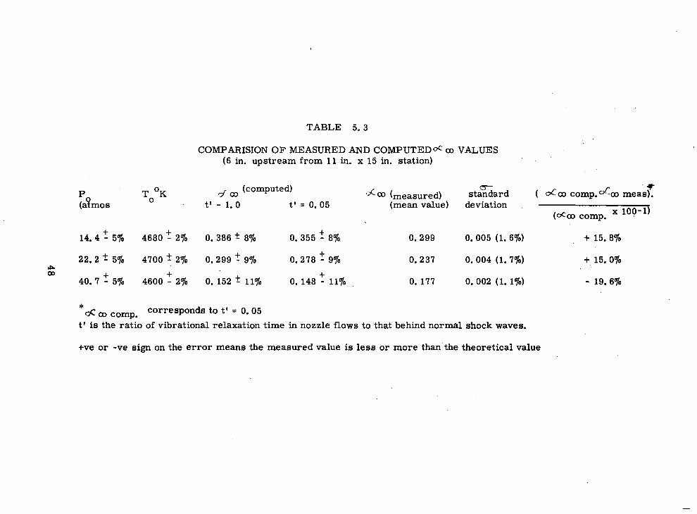
TABLE 5.3

COMPARISION OF MEASURED AND COMPUTED’7C’ 00 VALUES (6 in. upstream from 11 in. x 15 in. station)

P (a?mos

TooK d o. (computed) s-Lo3 ( measured) stazard ( Oc. co camp. Go measr t.’ - 1.0 t’ = 0.05 (mean value) deviation

(403 camp. x 109-l)

14. 4 + 5% 4680f 2% 0.386 f 8% 0.355 + 8% 0.299 0.005 (1.6%) + 15.8%

22.2 f 5% 4700 f 2% 0.299 + 9% 0.278 + 9% 0.237 0. 004 (1.7%) + 15.0% l!Gi

40. 7 + 5% 4600 ‘r 2% 0. 152 + 11% 0. 148 + 11% 0.177 0. 002 (1. lo/O) - 19.8%

*‘Yc co camp. corresponds to t’ = 0.05 t’ is the ratio of vibrational relaxation time in nozzle flows to that behind normal shock waves.

+ve or -ve sign on the error means the measured value is less or more than the theoretical value

COMBINATION OF AXlSYMMETRK AND TWO-DIMENSIONAL PROBES

1.8

1.6

. I IE OPERATING REGIMES--\

t I I I I I I I --- 0 1 2 d3h* 3 4

FIG. 2-l VARIATION OF PROBE SENSITIVITY WITH DIAMETER RATIO

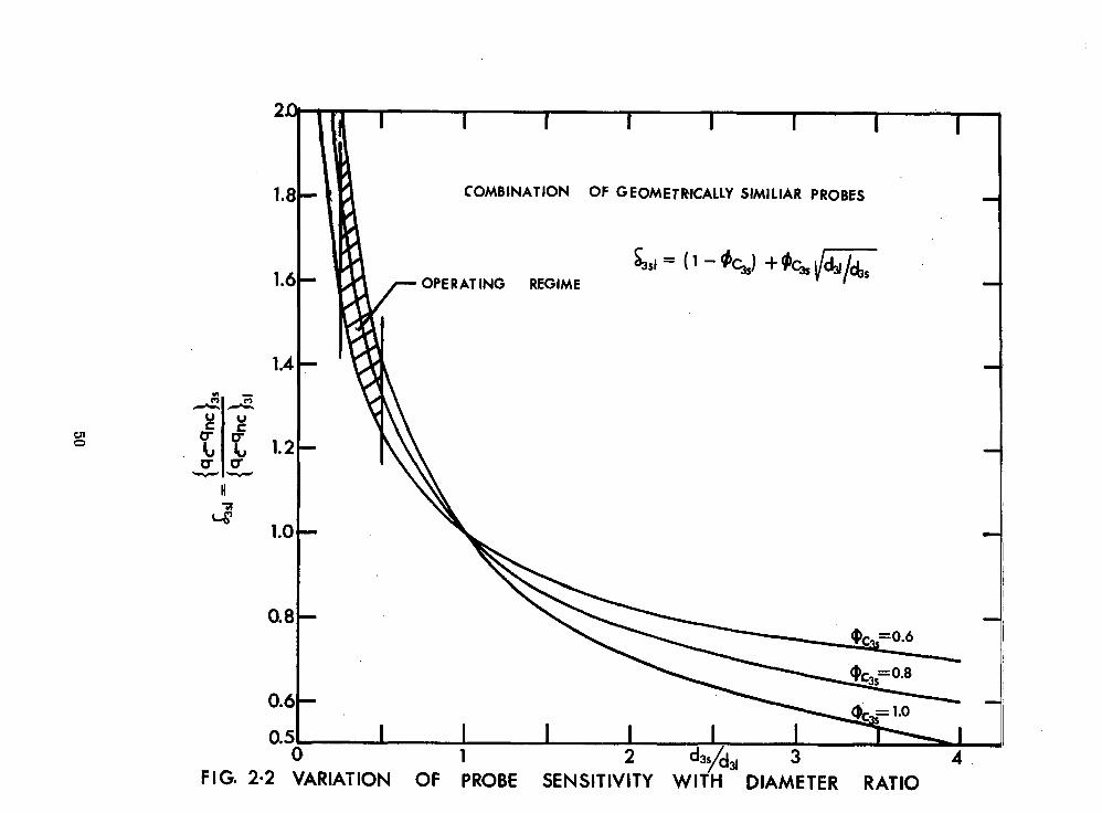
x

0.8

FIG. 2-2 VARIATION OF

COMBINATION OF GEOMETRiCALLY SIMILIAR PROBES

REGIME

I I I 1 2 4 PROBE SENSITIVIT ‘Y WIfH -- DIAMETER RATIO

I I I I I I I v

4/d,= 0.5 Average Value 2.05

-

Average Value O-73

2 5 10 20 50 lOA 2r10A 5x1 o- 10”

Re

FIG. 2.3 RATIO OF STANTON ‘NUMBERS IN LOW REYNOLDS NUMBER REGIME

SCHLIERFN SYSTEM

TIPw~n$ 17 TUNNEL

IVER n DR- ~~. I 1 - --v-----) --------- , - -+.----j---~----- I

BLOCK HCITTSF - [CONSOLE I- u _--- -_---- / INSTRUMENTS \/ I’ -- INSTRUMENTS

FIG. 3.1 GENERAL LAYOUT OF llin. x 15in. HYPERSONIC SHOCK TUNNEL

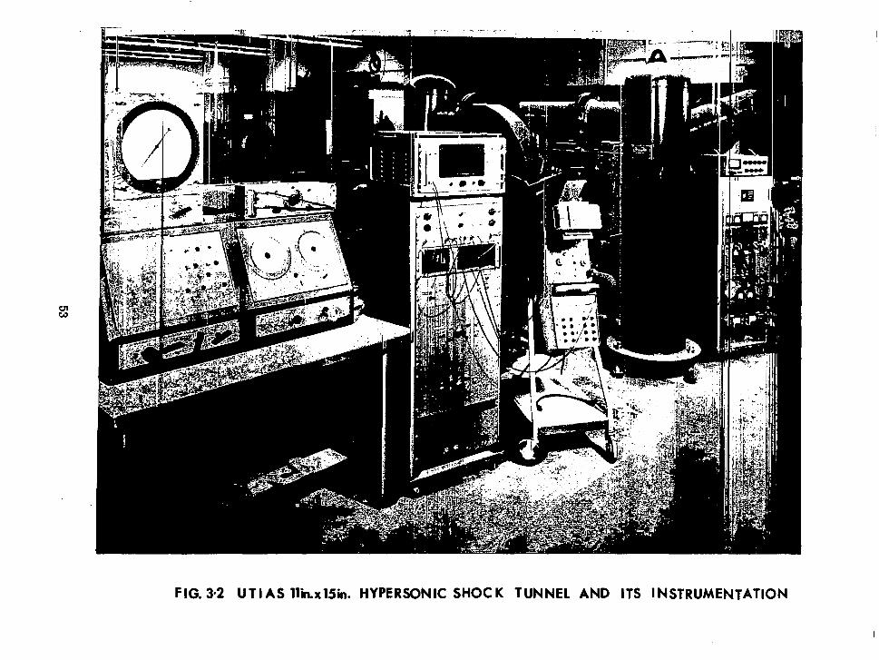
FIG. 3-2 UTI AS lh.xlSin. HYPERSONIC SHOCK TUNNEL AND ITS INSTRUMENTATION

II: 15” r-y1 urn t

------/L

I

RD EXPANSION

FIG. 3.3 AERODYNAMIC OUTLINE OF PRIMARY NOZZLE, CORNER EXPANSION PLATE AND FINAL NOZZLE OF THE! UTIAS llin. r 15in. HYPERSONIC SHOCK TUNNEL.

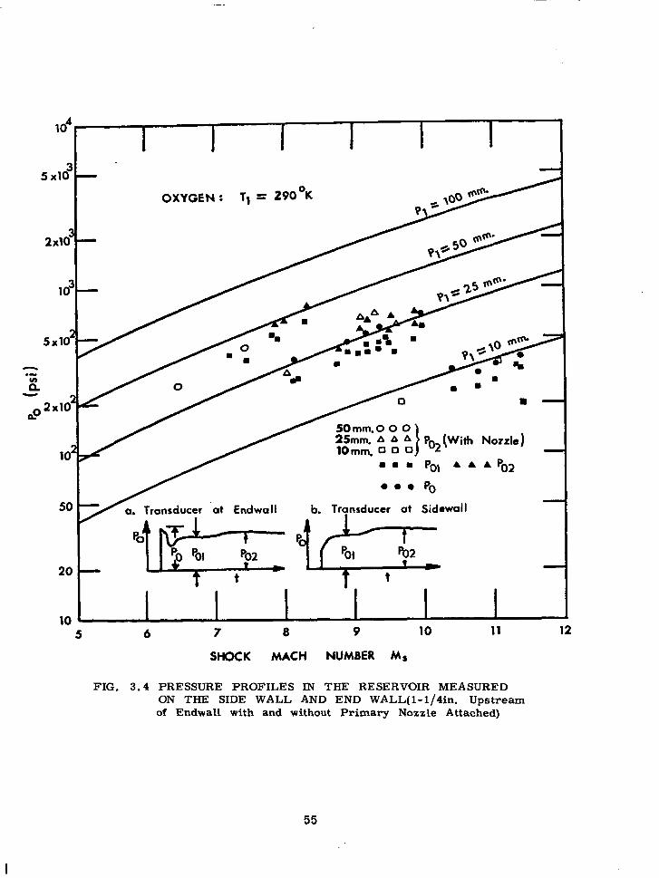
Bmm.0 0 0 imm. A A A --- PO-, (With Nozzle)

A A A PO2 10mm. u 0 UJ -a I” v

l mm POl

0.0 PO

a, Transducer ‘at Endwail b. Transducer at Sidewall

10 I I I I -

5 6 7 8 9 10 11 12

SHOCK MACH NUMBER M,

FIG. 3.4 PRESSURE PROFILES lN THE RESERVOIR MEASURED ON THE SIDE WALL AND END WALL(l-1/4in. Upstream of Endwall with and without Primary Nozzle Attached)

55

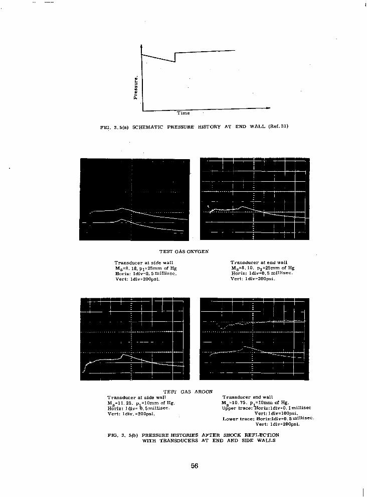
I Time

FIG. 3.5(a) SCHEMATIC PRESSURE HISTORY AT END WALL (Ref. 31)

TEST GAS OXYGEN

Transducer at side wall M,=8. 18, pl=25mm of Hg Horiz: Idiv=Cl. 5 millisec. Vert: ldiv=200psi.

Transducer at end wall M,=S. 10. pl=25mm of Hg Horiz: ldiv=O. 5 millisec. Vert: ldiv-200psi.

TEST GAS ARGON Transducer at side wall Transducer end wall M,=ll. 25. p =lOmm of Hg. Horiz: lcjiv= .5 millisec. b ~~~~~;~~,~~~~~~~~=~.l millisec Vert: ldiv. =2OOpsi. Vert: ldiv=lOOpsi.

Lower trace: Horiz:ldiv=O. 5millisec. Vex-t: ldiv=200psi.

FIG. 3. 5(b) PRESSURE HISTORIES AFTER SHOCK REFLECTION WITH TRANSDUCERS AT END AND SIDE WALLS

56

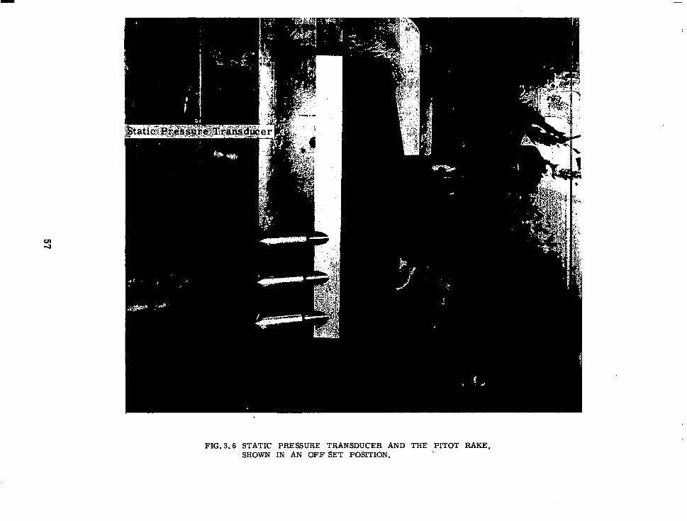
FIG. 3.6 STATIC PRESSURE TRANSDUCER AND THE PITOT RAKE, SHOWN IN AN OFF SET POSITION.

P ITOT PRESSURE x lo3 -- I 1.8 p6 t

ox-

- - - - -

-- 0.8

-- 0.6

-5 -4 -3 -2 -1 +l +2 +3 +4 +5

HORIZONTAL DISTANCE X ( inches)

FIG. 3-7 PITOT PRESSURE DISTRIBUTION IN THE TEST SECTION {llin. centreline)

-

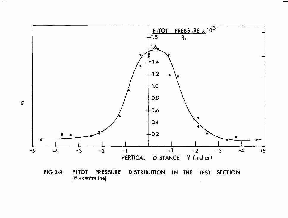
I PITOT PRESSURE x lo3

i-1.8 PO

-1 +l +2 +3 +4 +5 VERTICAL DISTANCE Y (inches )

FIG. 3.8 PITOT PRESSURE DISTRIBUTION IN THE TEST SECTION {15hcentreline)

FI :G. 5.1 AXISYMMETRIC AND TWO- DIMENSIONAL PROBES (d3/d,=Os

60

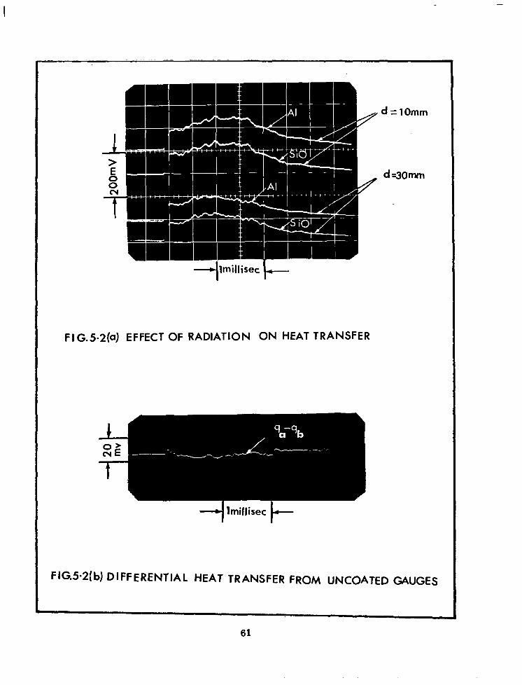
I

-I lmillisec I--

FIG.5.2(0) EFFECT OF RADIATION ON HEAT TRANSFER

FIG52:b) DIFFERENTIAL HEAT TRANSFER FROM UNCOATED GAUGES

61

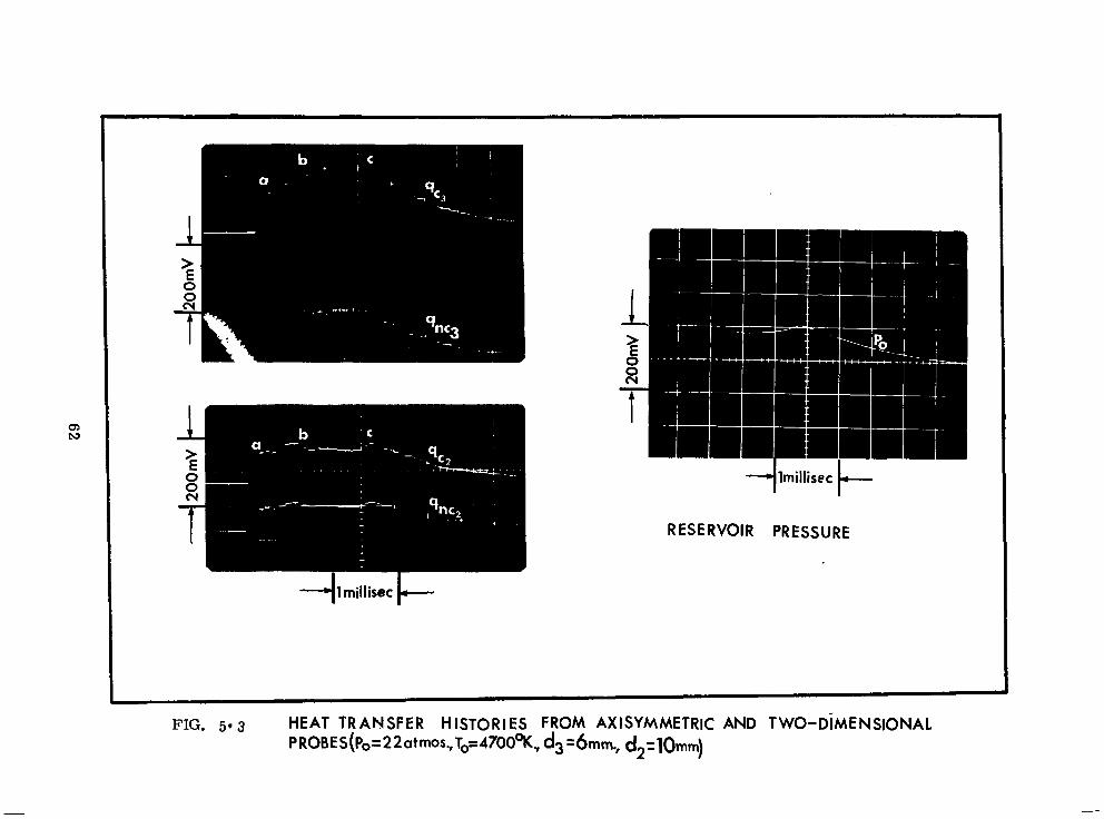
+nillisec k

RESERVOIR PRESSURE

FIG. 5.3 HEAT TRANSFER HISTORIES FROM AXISYMMETRIC AND TWO-DiMENSIONAL PROBES(Po=22atmos.,To=4700q<, da=6mm., d,=lOmm)

-

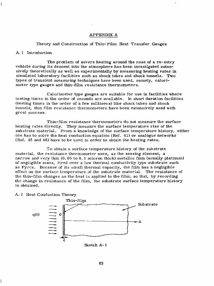
APPENDIX A

Theory and Construction of Thin-Film Heat Transfer Gauges

A. 1 Introduction

The problem of severe heating around the nose of a re-entry vehicle during its descent into the atmosphere has been investigated extensively theoretically as well as experimentally by measuring heating rates in simulated laboratory facilities such as shock tubes and shock tunnels. Two types of transient measuring techniques have been used, namely, calorimeter type gauges and thin-film resistance thermometers.

Calorimeter type gauges are suitable for use in facilities where testing times in the order of seconds are available. In short duration facilities (testing times in the order of a few millisecs) like shock tubes and shock tunnels, thin film resistance thermometers have been extensively used with great success.

Thin-film resistance thermometers do not measure the surface heating rates directly. They measure the surface temperature rise of the substrate material. From a knowledge of the surface temperature history, either one has to solve the heat conduction equation (Ref. 41) or analogue networks (Ref. 45 and 46) have to be used in order to obtain the heating rates.

To obtain a surface temperature history of the substrate material, the resistance thermometer uses, as the sensing element, a narrow and very thin (0.05 to 0. 1 micron thick) metallic film (usually platinum) of negligible mass, fired over a low thermal conductivity type substrate such as Pyrex. Because of its small thermal capacity, the film has a negligible effect on the surface temperature of the substrate material. The resistance of the thin-film changes as the heat is applied to the film; so that, by recording the change in resistance of the film, the substrate surface temperature history is obtained.

A. 2 Heat Conduction Theory

Thin-film

q(t)

Sub strate

Sketch A- 1

63

In genersl, the problem of heat conduction through a thin-film heat transfer gauge involves a solution of the heat conduction equation in a non- homogeneous body with dissimilar thermal and physical properties. However, by making some simplifying assumptions based on properties of the thin-film and the substrate, it has been shown in Ref. 41 that the measured temperature is essentially the surface temperature of the substrate. This means that the thin film offers negligible thermsl lag. Then the problem reduces to that of heat conduction through a homogeneous body involving only the thermal and physical properties of the substrate material. The assumptions made in reaching the above conclusions are worth noting

1) The thickness of the thin-film is very small.

2) The thermal conductivity of the thin-film (platinum) is much greater than that of the substrate material.

3) The time intervals of interest are large in comparison with the characteristic heat diffusion time across the thin-film. For example, for a time interval of 100 j-4 sets and one micron thick platinum resistance element, the ratio of time interval to heat diffusion time across the thin film is 2500 (Ref. 41).

The theory of heat conduction in the substrate material can be based on the one-dimensional model illustrated in Sketch A-l for the following reasons. The thickness of the thin-film is small and hence the edge area is orders of magnitude smaller than the planform area. Consequently, the lateral heat flow will be correspondingly small compared with the longitudinal heat flow. The substrate material can be assumed to be infinitely thick because the temperature of the rear face of a l/16-inch-thick slab of glass, subjected to a constant rate of heat transfer for two millisecs, would be less than 10m5% of the temperature on the front face and would be of the same order as the temperature l/16-inch below the surface of a semi-infinite body (Ref. 41).

The heat conduction equation for the substrate material with a time-dependent rate of heat transfer into the body is

ps cs c3e(x, t)/d t = k, a2 9(x, t)/bx2 (A. 1)

PS cs and k, are the density, specific heat and heat conductivity of the substrate material respective1 y.

6(x, t) is the surface temperature rise at a point x at a time t.

The appropriate boundary conditions are

ax, t) =O for x20; t=O e(x, t) = e,(t) for x = 0; t & 0 Lim 6(x, t) - 0

x--t+ a3

(A. 2)

64

The heat flux through unit area of the plane x = 0, which is sought in this problem, is

q(t) = - ks aebb t)ld t 1

(A. 3) x= 0

Applying Laplace transformation to Eq. (A. 1) and using boundary conditions (A. 2), one obtains a solution to the surface temperature as (Ref. 41)

t

ek t) = (1 /y S) f

qo\) (t- A+/2 exp I[

- x2/4(t -h)] [Ps cs /k a

dX (A. 4)

0

where h is a dummy variable and 9’ s = (srkpc>, 112

For x = 0, Eq. (A. 4) becomes the surface temperature response to a varying heat flux q(t)

t

e(t) = l@'S /

0) dX o (t -w2

(A. 5)

Since the surface temperature history is measured by a thin-film heat transfer gauge, Eq. (A. 5) must be arranged so that the unknown heat transfer rate q(t) is expressed as a function of e(t).

Again applying a Laplace transformation to both sides of Eq. (A. 5) and simplifying, one obtains a solution for q(t) as

t

q(t)= y’s d e(X) T dt / 0 (t - i)lE dX

(A. 6)

For complete derivation of Eqs. (A. 4 to A. 6), Ref. 41 may be consulted.

Equation (A. 6) is the analytical expression relating the surface temperature history to the applied heating rate. However, Eq. (A. 6) is not easy to solve and involves the use of a high-speed computer. The technique of measuring heat transfer directly by using analogue networks is given in Appendix B.

A. 3 Thin- Film Firing Technique

Liquid Bright Platinum* (Hanovia 05-X) is used widely for producing thin-film resistance thermometers. It is essentially a solution, in volatile oils and other solvents, of organic platinum and gold compounds of resinous character. When painted on a glazed ceramic surface and heated to maturity it yields a film of high polish like a mirror. The fired film has the colour of platinum metal. Besides the precious metals bright platinum contains

* This compound is manufactured and sold by Engelhard Industries Inc., Hanovia Liquid Gold Division, 1 West Central Avenue, East Newark, New Jersey, U. S. A.

65

some base metal-organic compounds which serve as fluxes to fix the metal firmly on glass or ceramics.

To fire the platinum film on Pyrex glass the following procedure proved to be successful. The Pyrex glass surface was first cleaned with alcohol or toluene and then any oily film on the surface was removed by cleaning the surface with a lint free cloth moistened with acetone. A film of Hanovia 05-X was then drawn between the lead wires using a drafting pen. The thickness of the film was controlled by thinning the Hanovia 05-X paint with acetone before it was applied. Then the film was fired on to the Pyrex surface by heating it in a precision furnace**. The temperature in the furnace was raised at the rate of 200°F/min until the firing temperature was reached. During this time the furnace door was slightly opened, so that all the volatile vapours were dispersed. The firing temperature (1250OF for Pyrex recommended by manufacturer) was set before the furnace was put on by using a set-point adjustment with a temperature indicator. When the firing temperature was reached, the door was closed and the film was fired for 4 minutes. The furnace was then turned off and the door opened. The Pyrex substrate was allowed to cool down for about 5 minutes inside the furnace. The rate of heating and firing time proved to be important in obtaining a pinhole free film surface. Also the film was exposed to indirect heating by keeping it near the top surface of the furnace where there were no heating coils.

The resulting film was opaque and had a mirror like surface. The film if properly fired wouH not be readily scratched even by a sharp object.

A. 4 Fabrication of Axisymmetric and Two-Dimensional Probes

In the fabrication of thin film heat transfer gauges, the least reliable elements is the electrical contact between the external leads and the thin-film. The use of conducting paint or solder often opens the contact between the thin film and the lead and also is a potential source of noise. This was avoided in the case of axisymmetric probes by imbedding platinum wires in Pyrex (#7740) rods (Fig. A. 1). Platinum wires were held in position inside a 5 mm 0. D. Pyrex tube and one end of the tube was melted so that about 10 mm length of the tube was formed into a solid rod. When the tube was cooled, the platinum wires were firmly secured in place in the solid portion of the tube. The outside diameter of the rod was formed equsl to the original diameter of the tube (5mm. 0. D. ) using a die. The solid end was ground and optically polished to the desired radius (this was done by Applied Physics Specialities Ltd., Don Mills, Ontario). In the process of grinding and polishing, the platinum wires sealed in the glass were also ground away, expos- ing bare ends flush with the glass surface. Then the thin film was painted between the bare ends and fired. During the firing process the thin-film made a good bond with the bare ends of platinum wire. These glass pieces were used as inserts in

t-s* The furnace is manufactured by L. J. Products 7464 Girard Avenue, La Jolla, California, U. S. A.

66

metal probes (Fig. 5.1) and could also be used more than once by grinding and polishing.

In the case of two-dimensional probes, the process described previously was not feasible since there were no grinding and polishing tools to generate a cylindrical surface. However, a truncated cylindrical piece cut from Pyrex (#7740) rod, and attached to a parsllelopiped plate glass (Fig. A. 1) using Plyabond adhesive, was used as the two-dimensional gauge insert. Platinum wires were attached to the thin-film by firing silver paint (Conductive Adhesive #1109, made by Electra. -Science Laboratories Inc., Philadelphia). Resistance of the platinum film was checked before and after the leads were attached, and gauges which showed any discrepancy were discarded. The exposed portion of the silver paint was coated with a thin coat of glyptol to avoid any possibility of shorting and noise.

A. 5 Heat Transfer Gauges Coating Technique

A vacuum evaporation process was used to deposit thin-films of silicon monoxide and silver on platinum films. All coatings were done usingtheplant at Applied Physics Specialties Ltd. Don Mills, Ontario. This plant consists of two separate diffusion pumps and two 18 in. bell jars. One is uced for the evaporation of metal films and the other for dielectrics. The ultimate vacuum was approximately 10-5 mm Hg. Transparent coating thicknesses (SiO) were estimated by colour and intensity changes of reflected white ligbt (visual). Metallic coating thickneesses were estimated from the amount of metal loading on coils.

Silicon monoxide was evaporated by keeping the substrate at 3ooOc. A 10, OOOOA thick coating was done at the rate of approximately lOOOA/min.

Silver was evaporated from a molybdenum boat. The substrate was heated to 20’O°C and then cooled down to 100°C before evaporation. A 2000°A thick coating was done at the rate of approximately 17OA/sec.

67

?iT *.. . Pyrex B&e

Silicone Monoxide Coating (Noncatalytic and lnsubting Surface) 10% Thick(l@)

Platinum Film Gauges 500°A To 750°A Thick

Silver Coating (Catalytic Surface) 2 000% Thick

Platinum Wires Embedded In Pyrex Bose ,

I -

s, -

Analogue ’ Networks

\

6~7m1n. --I- l!jin.

L

‘(a ) (b)

a) Two-dimensional Heat-transfer Gauge Insert

bj Axisymmetric Heat-transfer Gauge Insert

FIG. A. 1 CONSTRUCTION DETAILS 0 F CATALYTIC PROBES

68

APPENDIX B

Electrical Anslogue Network

B. 1 Introduction

It is noted in Appendix A, that numerical integration is necessary to obtain the heat transfer rate from the measured surface temperature history. This may be carried out by a suitably programmed digital computer, but the input data for the programme must be obtained from oscilloscope records of surface temperature histories. This process is time consuming and often leads to large errors. However, it was realized by Skinner (Ref. 45) and Meyer (Ref. 46) that electrical analogues of a heat conducting slab could be constructed which, if driven by a voltage proportional to surface temperature, would yield a signal proportional to the heat transfer rate.

B. 2 Analogy Between Heat and Current Conduction

The basis for constructing an electrical analogue of a heat conducting system arises from the identical forms of the equations for heat conduction and the diffusion of electrical charge in a system in which there is uniformly distributed resistance and capacitance. This analogy for a one- dimensional, semi-infinite, heat conducting slab is illustrated in Fig. B. 1. The governing equations for heat and current conduction (see Fig. B. 1) can be reduced to identical forms by using suitable non-dimensional quantities (Ref. 43), and a relation between the heat transfer and the current i s derived and is given in Fig. B. 1. Because of the difficulty of constructing an electrical model in which the capacitance and the resistivity are distributed, it is usual to approximate this by employing a network with lumped components. The commonly used T-section network is shown in Fig. B. 1. The current through the network is measured as a voltage drop across the first resistance of the network. Then, using the relation between the heat transfer and the current (given in Fig. B. l), an expression for heat transfer can be derived and is given by,

Q(t) = u~/&~, cyf D$ I[

(kpc),/RC 1 “2 (B. 1)

where Dl is the amplification factor of the preamplifier if any.

B. 3 Design of an Analogue Network

The T-section network as shown in Fig. B. 1 was selected for reasons outlined in Ref. 46. uq is proportional to (RC)l/2,

For a given heat transfer q(t), the output voltage whereas the response time of the system is

given by RC, so that in general it is necessary to make some compromise between fast response and an adequate output signal level. The network must be made long enough so that for the time during which measurements are made the system behaves as though it were semi-infinite. It was shown in Ref. 46

69

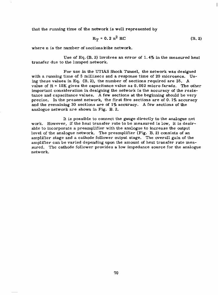
that the running time of the network is well represented by

RT=0.2n2RC 03.2)

where n is the number ofsectionshthe network.

Use of Eq. (B. 2) involves an error of 1.4% in the measured heat transfer due to the lumped network.

For use in the UTIAS Shock Tunnel, the network was designed with a running time of 5 millisecs and a response time of 20 microsecs. Us- ing these values in Eq. (B. 2), the number of sections required are 35. A value of R = 10K gives the capacitance value as 0.002 micro farads. The other important consideration in designing the network is the accuracy of the resistance and capacitance values. A few sections at the beginning should be very precise. In the present network, the first five sections are of 0. 1% accuracy and the remaining 30 sections are of 1% accuracy. A few sections of the analogue network are shown in Fig. B. 2.

It is possible to connect the gauge directly to the analogue net work. However, if the heat transfer rate to be measured is low, it is desirable to incorporate a preamplifier with the analogue to increase the output level of the analogue network. The preamplifier (Fig. B. 2) consists of an amplifier stage and a cathode follower output stage. The overall gain of the amplifier can be varied depending upon the amount of heat transfer rate measured. The cathode follower provides a low impedance source for the analogue network.

70

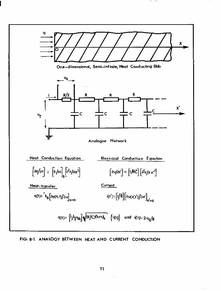
One-dimensional, Semi-infinite, Heat Conducting Sk&

-us- . .

Analogue Network

Heat Conduction Equation

I Heat-transfer

Electrical Conduction Eauation

Current

q(t)= [i/~~]$R/c)(kpc& ’ ii(t)} ad i(t)=sUq/R

FIG. B-1 ANALOGY BETWEEN HEAT AND CURRENT CONDlJCTlON

71

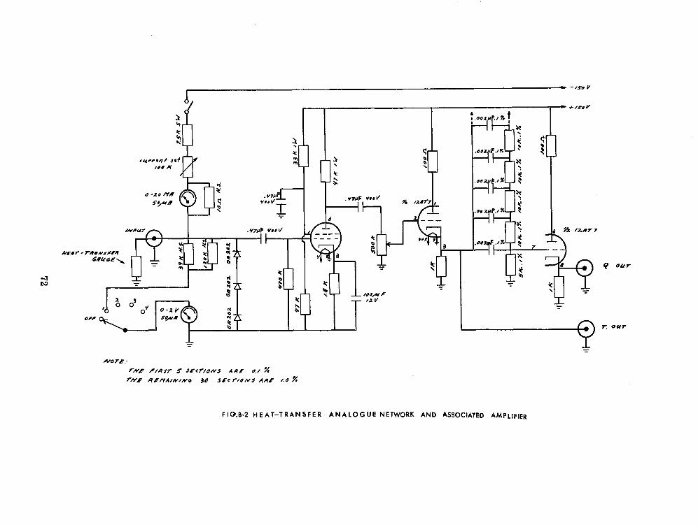
FIC~.B.? HEAT-TRANSFER ANALOGUE NETWORK AND ASSOCIATED AMPLIFIER

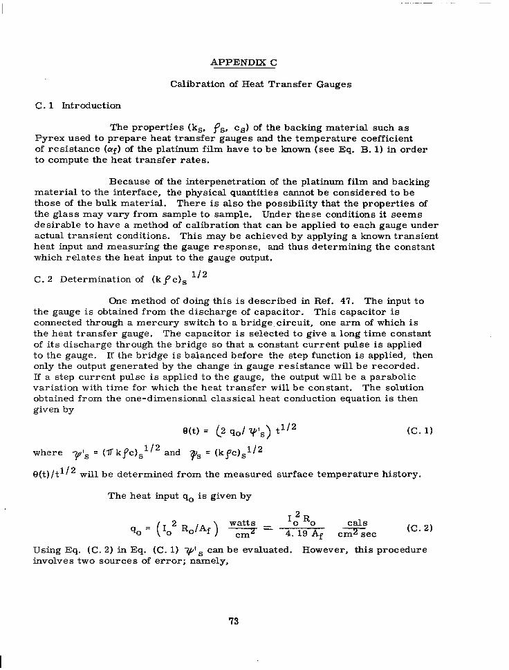
APPENDIX C

Calibration of Heat Transfer Gauges

C. 1 Introduction

The properties (k,, ps, c,) of the backing material such as Pyrex used to prepare heat transfer gauges and the temperature coefficient of resistance (cuf) of the platinum film have to be known (see Eq. B. 1) in order to compute the heat transfer rates.

Because of the interpenetration of the platinum film and backing material to the interface, the physical quantities cannot be considered to be those of the bulk material. There is also the possibility that the properties of the glass may vary from sample to sample. Under these conditions it seems desirable to have a method of calibration that can be applied to each gauge under actual transient conditions. This may be achieved by applying a known transient heat input and measuring the gauge response, and thus determining the constant which relates the heat input to the gauge output.

C. 2 Determination of (kpc), l/2

One method of doing this is described in Ref. 47. The input to the gauge is obtained from the discharge of capacitor. This capacitor is connected through a mercury switch to a bridge.circuit, one arm of which is the heat transfer gauge. The capacitor is selected to give a long time constant of its discharge through the bridge so that a constant current pulse is applied to the gauge. If the bridge is balanced before the step function is applied, then only the output generated by the change in gauge resistance will be recorded. If a step current pulse is applied to the gauge, the output will be a parabolic variation with time for which the heat transfer will be constant. The solution obtained from the one-dimensional classical heat conduction equation is then given by

e(t) = (2 9oJ VI,) A2 (C. 1)

where Y’s = (flkpc)s1’2 and pl, = (kpc),l12

e(t)/&2 will be determined from the measured surface temperature history.

The heat input q. is given by

( 12Ro/Af) 5= CR0 cals

qo= 0 4.19Af ---2-=- cm set tc. 2)

Using Eq. (C. 2) in Bq. (C. 1) y’s can be evaluated. However, this procedure involves two sources of error; namely,

73

1) The area of the film (Af) must be known and is often very difficult to measure accurately.

2) The bridge must be perfectly balanced and is very difficult to do in practice.

Using the above technique, the quantity F Is could only be determined with an accuracy off 18% (Ref. 41).

In order to eliminate the preceding errors, Skinner (Ref. 48) has developed a new method. In this method, a step current is applied to the gauge and the surface temperature rise is recorded. The gauge is then immersed in a water bath so that the exposed side of the film is in contact with water. The step current is again applied and heat flows both into the glass and into the water. The temperature rise is again recorded.

These two temperature records have the same time dependence (if the bridge balance remains the same) but different amplitudes. The ampli- tude ratio is simply related to the ratio of the yls of the backing material and water.

A thin-film gauge adopts the surface temperature of its backing material. When pulsed in air, this temperature is related to the flux of heat through the surface by the simple equation (from Eq. A. 6).

q= Y’s f(t) (C. 3) 7T

where, f(t) = surface temperature function

Equation C. 3 assumes one-dimensional heat flow into the glass and neglects any heat flux into the air in contact with the other side of the gauge.

Then the gauge is immersed in a water bath at the same initial temperature, and the same current pulse is passed through it. Heat will flow both into the glass and .into the water. Here the very reasonable assumption is made that the gauge presents the same effective area to both glass and water. The total heat flux which is dissipated into the backing material as well as into the water is given by

q= J$ !W f%) + + f*(t)

where * corresponds to quantities pulsed in water.

i& = bkfc)s+‘2 for water

Equating right hand sides of Eqs. (C. 3) and (C. 4) gives

tc. 4)

v’,f(t) = (Tls + u”,) f*(t) (C. 5).

74

The functional form of f(t?must be the same since the same current pulse is applied in both cases. i. e.,

Therefore, we can write f(t) = Bf,(t) and f*(t) = B*f,(t) f(t) and f*(t) differ only in magnitude.

Equation C. 5 can be rewritten as

(or)

?$, B = tyls + ytw> B*

-@‘S = yfw [(B/B*) - I] -’ (C. 6)

Thus, if the gauge is pulsed in air and in water, then the gauge constants can be computed from Eq. (C. 6) by taking the ratio of the amplitudes of the gauge outputs at a certain time.

The bridge used in this technique is a simple Wheatstone bridge to which a step function is applied as a driving voltage. When one arm of the bridge is a thin-film gauge and the other arms are purely resistive, the bridge cannot be accurately balanced. This is a major source of error. The problem of bridge balancing is dealt with in detail in Ref. 48. However, if the above method (water bath technique) is used, considerable unbalance in the bridge can be tolerated (since the absolute values of the gaug.e output are not involved) provided the same unbalance can be maintained when the gauge is pulsed in air and in water. This in practice is very difficult to achieve because the resistance of the gauge, when immersed in water, changes slightly. This change in resistance is often small for coated gauges. But this slight change in resistance introduces considerable error in the ratio of gauge outputs Fig. C. l(b) . Also the thin-film resistance changes by different amounts due to heating, when pulsed in air and in water, which in turn introduces different amounts of unbalance in the bridge.

The following procedure may be followed in order to correct for the preceding effects.

In general, if the bridge is not properly balanced, then applying a step current pulse to it produces a step function signal, superimposed on the expected parabolic signal from the gauge as shown in Fig. C. l(a). If such an output from the gauge is fed to the analogue network and the heat transfer is measured, then the input to the analogue (Ref. 43) is

T=D+ETlJ2=~+ f (C. 7)

where T=~,/Tr=UT/Uo, f=0,/T, =uT/Uo, YL’t/t,

and the output from the anslogue is

112 a = D/(lr?#2 + Tl- E/2

75

and

where

6 = (2/Uo)(to/RC)1’2,q(t)

From Eq. (C. 8) 4TT

112 l-J=- -

UO

t(t/RC)1’2

Then from Eq. (C. 7)

or u =u

T T + 4t (flt/RC)

(C. 8)

(C. 9)

(C. 10)

(C. 11)

Even, if the bridge balance (or unbalance) changes when the gauge is pulsed in water, the unblanced output (ET) from the gauge can be corrected by using equation (C. 11).

When the gauge is pulsed either in air or in water the output signal is fed to the analogue and output from the analogue is measured as shown in Fig. C. l(b). Note that the heat transfer continuously decreases instead of keeping constant with time due to unbalance, and also the rate of decrease of heat transfer when the gauge is pulsed in air is slightly different from the one in water. At any given time the surface temperature signal (TT) and slope of the corresponding heat transfer signal [diiq(t)/dt] are obtained from the oscilloscope traces Fig. C. l(b) . Then the true signal (UT) is determined from Eq. (C. 11). This correction was applied for both signals with the gauge pulsed in air and in water.

Using this t chnique, the heat transfer gauges were calibrated and the value of ( kpc)S 172 was found to be 0.0750 27% BTU ftW2 OF-l set- l12. In order to test the above method of correction, the bridge was deliberately left at different levels of unbalance in some cases and the surface temperature and heat transfer were recorded. In all these cases the correction could be

The value of (kpc) l12.for water is 0.078

The temperature coefficient of resistance of platinum film (of) was determined by immersing the heat transfer gauge in a hot oil bath and the resistance of the film was measured accurately at different temperatures. The heat transfer gauge was protected by placing the gauge in a test tube which in turn was immersed in the hot oil bath. The variation of resistance with temperature was found to be linear in the temperature range of 25’C to 100°C. The slope of this line gave cuf. A value of crf = 1.21 x 10m3 JL /fi°F represented a good average for all the gauges with an error of 2 2.5%, which includes the error due to cuf change with temperature.

76

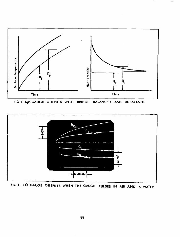
Time

t “q 6

Time

FIG. C-l<a> GAUGE OUTPUTS WITH BRIDGE BALANCED AND UNBALAklED

FIG.CMb> GAUGE OUTPUTS WHEN THE GAUGE PULSED IN AIR AND IN WATER

77

APPENDIX D

Error Estimation in Measurement of qc and crao

D. 1 Introductory Remarks .

To estimate the absolute error involved in measuring q c and CX~, the fundamental principles, outlined in the “Introduction to the Theory of Error” by Y. Beers (Ref. 49) are extensively used. Some of the principles are noted below.

a) All the errors are classified either independent and dependent errors,

b) In the case of independent errors the logical way of adding the separate contributions is to take the square root of the sum of their squares. This procedure is too conservative and some research workers reduce the total error, perhaps by one-third.

c) In the case of dependent errors the rule is to replace the square root of the sum of squares addition by algebric addition.

D. 2 Heat Transfer

The heat transfers were measured by using an analogue network (Appendix B) and a Tektronix-565 scope. The specific expression used was

q(t) = [2 u Ku q 90 of Dl)] IkPcWRC] 1’2 (D. 1)

The error due to the finite size of the analogue network is negligible (Ref. 46) and the value of RC can be taken as quite accurate since the value of R and C in the network are of 0.1% accuracy.

Then i As/q) = Auq/ug + A~J7& - n@fl@f 03.2)

There are two errors involved in measuring uq namily: the scope accuracy which is _ + 3% and the error in reading the heat transfer traces, which is approximately ? 3%. error, which is 27% (see Appendix C).

The error inys is the gauge calibration The error in af is also the gauge

calibration error, which is 2 2.5% (see Appendix C). All these errors are independent of each other, so that the total error is given by the square root of the sum of their squares. Thus

hq= q

(au,/,); + (b~s@‘s)2 + ( Aafk)2 I

l/2 0.3)

= t + 3%12 + t + 3%)2 + ( + 7%)2 + <+ 2.5%)2 (D. 4)

z 8.6%

78

Since this procedure is too conservative, the most probable error is taken as 213 of 8.6 70 = 5.7%.

D. 3 Catalytic Efficiency (e)

The catalytic efficiency is given by

+c3 = G qc3 - qnc3 _ 1

qc3 - qnc3 1 03.5)

-1 with G= (2d2/d3)1’2 - l]

Since the catalytic efficiency is a function of only the measured quantities (apart from the diameter ratio which is’s constant) some of the errors involved in measuring the heat transfers become dependent in this particular application. The errors involved in measuring the heat transfers except the reading error become dependent because all the heat transfer measurements were done by using the same scope, same batch of backing material and all the platinum films were fired under identical conditions. The reading error is subject to individual judgement and it is most probable that the error is committed in an independent manner.

Then the errors in 8, due to dependent and independent errors will be computed separately using the rules metnioned before and these two errors will be combined by taking the square root of the sum of their squares.

Since the dependent errors are added algebricdlly, the error in 0, due to dependent errors can be written as (Ref. 49)

1 03.6)

Since the error in measuring all the heat transfers is the same, it is apparent from Eq. (D. 6) that

Ah3 - L I =o 0 c3

The error due to the independent error can be written as

79

0.7)

(D. 8)

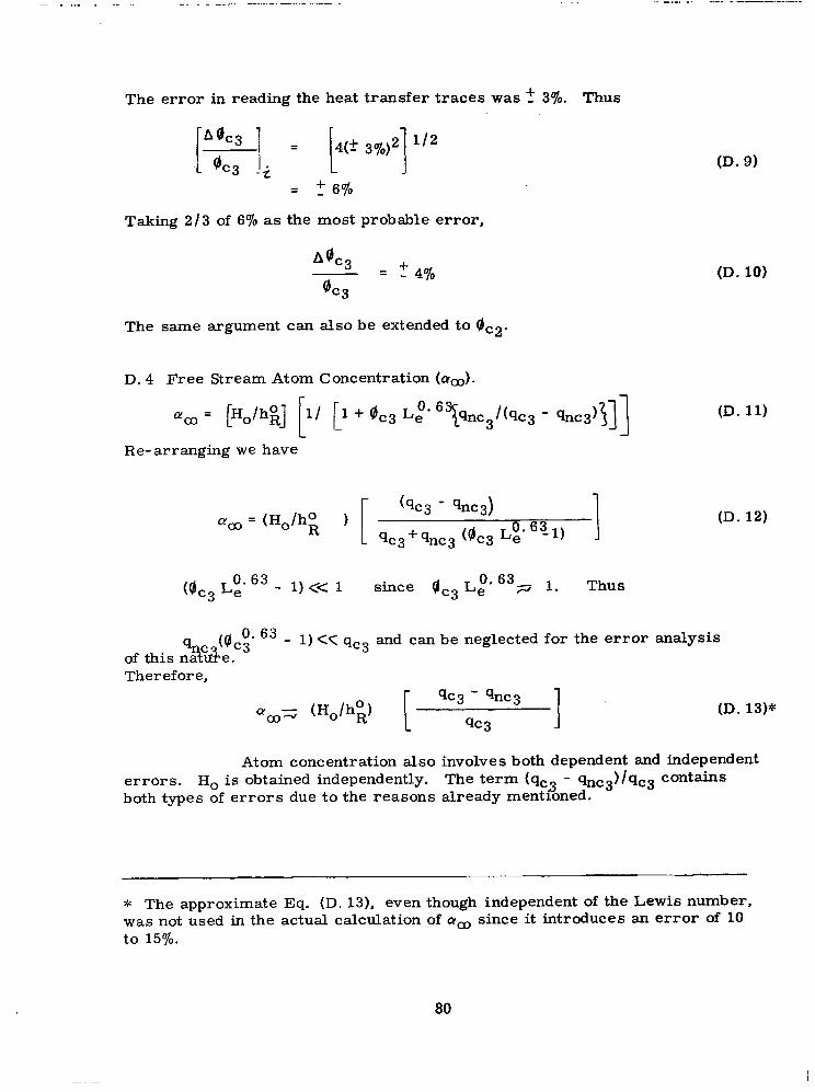
The error in reading the heat transfer traces was ? 3%. Thus

Ah3 1 = Ok, I. -2 = + 6%

Taking 2/3 of 6% as the most probable error,

A%3 -=

0cj + 4%

The same argument can also be extended to gc2,

D. 4 Free Stream Atom Concentration (cu&.

~00 = [Ho/h;] [Ii p + @cg L,O’ 6Tqnc3/(qc3 - qnc3)$]]

Re-arranging we have

ctcx) = (Ho/h; 1 (qc3 - qnc3)

qc3 +q nc3 (0,, LO,’ 631)

(D. 9)

(D. 10)

(D. 11)

(D. 12)

(0,, LE. 63 - 1) cc 1 since (Ic3 Li’ 63g 1. Thus

0. 63

of this &c%(!.c3 - 1) <c qc3 and can be neglected for the error analysis

Therefore,

qc3 - qnc3 “a= (Ho/ho,) 1 (D. 13)*

Atom concentration also errors. Ho is obtained independently. both types of errors due to the reasons

qc3 J

involves both dependent and independent The term tqc3 - 9nc3 )k3 contains already mentloned.

* The approximate Eq. (D. 13), even though independent of the Lewis number, was not used in the actual calculation of LT~ since it introduces an error of 10 to 15%.

80

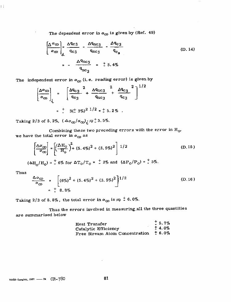
The dependent

Aqc3

qc3

error in aoo is given by (Ref. 49)

Aqnc 3 A%3 -- qnc 3 qc,

(D. 14)

Aqnc3 = - = + 5.4%

9 nc3

The independent error in aoo (i. e. reading error) is given by

2 2 112 Aqnc3 - =

r3, I

%+ ‘+ A=k3

. 9c3 qnc3 9c3 1 = + 3(f 3%)2 1’2 =-r 5.2% .

Taking 2’3 of 5. 2%, ( Aao3/am)i;3+3. 5%.

Combining these two preceding errors with the error in Ho, we have the total error in ao., as

I I[ G = (~qgt (5.4%)2 + (3.5%)2 l/2 1 (D.15)

(AHo/Ho) = ? 6% for AT,/T, = f 2% and (APO/PO) = ? 5%.

Thus

(D. 16 1 4ao3 -= aco

(6%)2 + (5. 4%)2 + (3. 59’0)~ 1’2 J = + 8.870

Taking 213 of 8.8%, the total error in am is = ? 6.0%.

Thus the errors involved in measuring-all the three quantities are summarised below

Heat Transfer + 5.7% Catalytic Efficiency + 4.0% Free Stream Atom Concentration 2 6.0%

NASA-Langley, 198? - 24 CR-780 81

Documents

by N MT. Reddy