Embed Size (px)
Citation preview

Compact Discrete Representations for Scalable Similarity Search
by
Mohammad Norouzi
A thesis submitted in conformity with the requirementsfor the degree of Doctor of Philosophy
Graduate Department of Computer ScienceUniversity of Toronto
c© Copyright 2016 by Mohammad Norouzi

Abstract
Compact Discrete Representations for Scalable Similarity Search
Mohammad Norouzi
Doctor of Philosophy
Graduate Department of Computer Science
University of Toronto
2016
Scalable similarity search on images, documents, and user activities benefits generic search, data
visualization, and recommendation systems. This thesis concerns the design of algorithms and
machine learning tools for faster and more accurate similarity search. The proposed techniques
advocate the use of discrete codes for representing the similarity structure of data in a compact
way. In particular, we will discuss how one can learn to map high-dimensional data onto
binary codes with a metric learning approach. Then, we will describe a simple algorithm for
fast exact nearest neighbor search in Hamming distance, which exhibits sub-linear query time
performance. Going beyond binary codes, we will highlight a compositional generalization of k-
means clustering which maps data points onto integer codes with storage and search costs that
grow sub-linearly in the number of cluster centers. This representation improves upon binary
codes, and provides an even more precise approximation of Euclidean distance. Experimental
results are reported on multiple datasets including a dataset of SIFT descriptors with 1B entries.
ii

Acknowledgements
I would like to thank my extraordinary advisor and mentor, David Fleet, for his continuous
support and encouragement, his perfectionism, clarity, great intuitions, openness to ideas, as
well as his chill attitude, modesty, and superb sense of humor. I was truly blessed to have David
as my teacher.
I am grateful to the rest of my advisory committee including Radford Neal, Ruslan Salakhut-
dinov, and Kyros Kutulakos, whose insightful comments and great questions inspired me to
extend some of the research findings and helped me improve the exposition of the ideas. I
am grateful to Thorsten Joachims and Raquel Urtasun for serving as my thesis examiners and
offering me their thoughtful comments and feedback.
I thank my fellow labmates and members of the AI group for stimulating discussions and
the fun we had together at UofT including Abdel-Rahman Mohamed, Aida Nematzadeh, Ali
Punjani, Amin Tootoonchian, Charlie Tang, Fartash Faghri, Fernando Flores-Mangas, George
Dahl, Ilya Sutskever, Jonathan Taylor, Kaustav Kundu, Marcus Brubaker, Navdeep Jaitly, Ni-
tish Srivastava, Sarah Sabour, Shenlong Wang, Siavosh Benabbas, Tom Lee, Varada Kolhatka,
Vlad Mnih, Wenjie Luo, Yanshuai Cao, Yuval Filmus, and others. I am sorry about forgetting
to include some of the names. You are going to be missed.
My sincere gratitude goes to Peyman Sarrafi and Ali Ashasi for putting up with me. My
thanks also goes to my awesome friends for cheering me up, including Afshar Ganjali, Ahmad
Sobhani, Ali Kalantarian, Ali Naseri, Alireza Sahraei, Amir Aghaei, Asghar Zahedi, Ebrahim
Bagheri, Emad Zilouchian, Faezeh Ensan, Hamed Parham, Hamideh Zakeri, Hossein Kaffash,
Kaveh Ghasemloo, Kianoosh Mokhtarian, Mandana Einolghozati, Mansour Safdari, Moham-
mad Derakhshani, Mohammad Rashidian, Mona Sobhani, Morteza Zadimoghaddam, Nima
Zarian, Safa Akbarzadeh, Samira Karimelahi, Zeynab Ziaie, and others that I forgot to include.
I particularly thank Nazanin Montazeri for her constant support and positive energy.
I thank Relu Patrascu for his interesting conversations and for keeping our computers and
servers up and running. I also thank Luna Keshwah for her excellent administrative support.
I express my deepest gratitude to my special family, my best parents in the world, Mansoureh
and Sadegh, and my best brothers in the universe, Mahdi and Sajad. My family supported me,
shared with me their advice, and made me feel unconditionally loved from oversees.
iii
Contents
1 Introduction 1
1.1 Nearest neighbor search . . . . . . . . . . . . . . . . . . . . . . . . . . . . . . . . 2
1.2 Keyword search in text documents . . . . . . . . . . . . . . . . . . . . . . . . . . 3
1.3 Hashing for nearest neighbor search . . . . . . . . . . . . . . . . . . . . . . . . . 4
1.4 Sketching with compact discrete codes . . . . . . . . . . . . . . . . . . . . . . . . 5
1.5 Our approach to learning hash functions . . . . . . . . . . . . . . . . . . . . . . . 7
1.6 Search in Hamming space . . . . . . . . . . . . . . . . . . . . . . . . . . . . . . . 8
1.7 Vector quantization for nearest neighbor search . . . . . . . . . . . . . . . . . . . 9
1.8 Thesis Outline . . . . . . . . . . . . . . . . . . . . . . . . . . . . . . . . . . . . . 10
1.9 Relationship to Published Papers . . . . . . . . . . . . . . . . . . . . . . . . . . . 10
2 Minimal Loss Hashing 12
2.1 Formulation . . . . . . . . . . . . . . . . . . . . . . . . . . . . . . . . . . . . . . . 13
2.1.1 Pairwise hinge loss . . . . . . . . . . . . . . . . . . . . . . . . . . . . . . . 14
2.1.2 Binary Reconstructive Embedding . . . . . . . . . . . . . . . . . . . . . . 14
2.2 Bound on empirical loss . . . . . . . . . . . . . . . . . . . . . . . . . . . . . . . . 15
2.2.1 Structural SVM . . . . . . . . . . . . . . . . . . . . . . . . . . . . . . . . 16
2.2.2 Convex-concave bound for hashing . . . . . . . . . . . . . . . . . . . . . . 16
2.2.3 Tightness of the bound and regularization . . . . . . . . . . . . . . . . . . 17
2.3 Optimization . . . . . . . . . . . . . . . . . . . . . . . . . . . . . . . . . . . . . . 18
2.3.1 Loss-augmented inference with pairwise hashing loss . . . . . . . . . . . . 18
2.3.2 Perceptron-like learning with pairwise loss . . . . . . . . . . . . . . . . . . 19
2.4 Implementation details . . . . . . . . . . . . . . . . . . . . . . . . . . . . . . . . . 21
2.5 Experiments . . . . . . . . . . . . . . . . . . . . . . . . . . . . . . . . . . . . . . . 21
2.5.1 Six datasets . . . . . . . . . . . . . . . . . . . . . . . . . . . . . . . . . . . 22
2.5.2 Euclidean 22K LabelMe . . . . . . . . . . . . . . . . . . . . . . . . . . . . 23
2.5.3 Semantic 22K LabelMe . . . . . . . . . . . . . . . . . . . . . . . . . . . . 26
2.6 Hashing for very high-dimensional data . . . . . . . . . . . . . . . . . . . . . . . 27
2.7 Summary . . . . . . . . . . . . . . . . . . . . . . . . . . . . . . . . . . . . . . . . 29
2.A Proof of the inequlity on the tightness of bound . . . . . . . . . . . . . . . . . . . 30
iv

3 Hamming Distance Metric Learning 31
3.1 Formulation . . . . . . . . . . . . . . . . . . . . . . . . . . . . . . . . . . . . . . . 32
3.1.1 Triplet loss function . . . . . . . . . . . . . . . . . . . . . . . . . . . . . . 33
3.2 Optimization through an upper bound . . . . . . . . . . . . . . . . . . . . . . . . 34
3.2.1 Loss-augmented inference with triplet hashing loss . . . . . . . . . . . . . 35
3.2.2 Perceptron-like learning with triplet loss . . . . . . . . . . . . . . . . . . . 36
3.3 Asymmetric Hamming distance . . . . . . . . . . . . . . . . . . . . . . . . . . . . 37
3.4 Implementation details . . . . . . . . . . . . . . . . . . . . . . . . . . . . . . . . . 37
3.5 Experiments . . . . . . . . . . . . . . . . . . . . . . . . . . . . . . . . . . . . . . . 38
3.6 Summary . . . . . . . . . . . . . . . . . . . . . . . . . . . . . . . . . . . . . . . . 41
4 Fast Exact Search in Hamming Space with Multi-Index Hashing 44
4.0.1 Background: problem and related work . . . . . . . . . . . . . . . . . . . 45
4.1 Multi-Index Hashing . . . . . . . . . . . . . . . . . . . . . . . . . . . . . . . . . . 47
4.1.1 Substring search radii . . . . . . . . . . . . . . . . . . . . . . . . . . . . . 47
4.1.2 Multi-Index Hashing for r-neighbor search . . . . . . . . . . . . . . . . . . 49
4.2 Performance analysis . . . . . . . . . . . . . . . . . . . . . . . . . . . . . . . . . . 50
4.2.1 Choosing an effective substring length . . . . . . . . . . . . . . . . . . . . 52
4.2.2 Run-time complexity . . . . . . . . . . . . . . . . . . . . . . . . . . . . . . 53
4.2.3 Storage complexity . . . . . . . . . . . . . . . . . . . . . . . . . . . . . . . 54
4.3 k-Nearest neighbor search . . . . . . . . . . . . . . . . . . . . . . . . . . . . . . . 54
4.4 Experiments . . . . . . . . . . . . . . . . . . . . . . . . . . . . . . . . . . . . . . . 56
4.4.1 Datasets . . . . . . . . . . . . . . . . . . . . . . . . . . . . . . . . . . . . . 58
4.4.2 Experimental results . . . . . . . . . . . . . . . . . . . . . . . . . . . . . . 59
4.4.3 Multi-Index Hashing vs. Linear Scan . . . . . . . . . . . . . . . . . . . . . 59
4.4.4 Direct lookups with a single hash table . . . . . . . . . . . . . . . . . . . 62
4.4.5 Substring Optimization . . . . . . . . . . . . . . . . . . . . . . . . . . . . 63
4.5 Implementation details . . . . . . . . . . . . . . . . . . . . . . . . . . . . . . . . . 64
4.6 Conclusion . . . . . . . . . . . . . . . . . . . . . . . . . . . . . . . . . . . . . . . 66
5 Cartesian k-means 68
5.1 k-means . . . . . . . . . . . . . . . . . . . . . . . . . . . . . . . . . . . . . . . . . 69
5.2 Orthogonal k-means with 2m centers . . . . . . . . . . . . . . . . . . . . . . . . . 69
5.2.1 Learning ok-means . . . . . . . . . . . . . . . . . . . . . . . . . . . . . . . 71
5.2.2 Distance estimation for approximate nearest neighbor search . . . . . . . 72
5.2.3 Experiments with ok-means . . . . . . . . . . . . . . . . . . . . . . . . . . 73
5.3 Cartesian k-means . . . . . . . . . . . . . . . . . . . . . . . . . . . . . . . . . . . 74
5.3.1 Learning ck-means . . . . . . . . . . . . . . . . . . . . . . . . . . . . . . . 77
5.4 Relations and related work . . . . . . . . . . . . . . . . . . . . . . . . . . . . . . 78
5.4.1 Iterative Quantization vs. Orthogonal k-means . . . . . . . . . . . . . . . 78
v
5.4.2 Orthogonal k-means vs. Cartesian k-means . . . . . . . . . . . . . . . . . 78
5.4.3 Product Quantization vs. Cartesian k-means . . . . . . . . . . . . . . . . 79
5.5 Experiments . . . . . . . . . . . . . . . . . . . . . . . . . . . . . . . . . . . . . . . 79
5.5.1 Euclidean distance estimation for approximate NNS . . . . . . . . . . . . 79
5.5.2 Learning visual codebooks . . . . . . . . . . . . . . . . . . . . . . . . . . . 82
5.6 More recent quantization techniques . . . . . . . . . . . . . . . . . . . . . . . . . 83
5.7 Summary . . . . . . . . . . . . . . . . . . . . . . . . . . . . . . . . . . . . . . . . 84
6 Conclusion 85
Bibliography 87
vi
List of Tables
3.1 Classification error rates on MNIST test set. . . . . . . . . . . . . . . . . . . . . . 39
3.2 Recognition accuracy on the CIFAR-10 test set . . . . . . . . . . . . . . . . . . . 41
4.1 Summary of run-time results on AMD machine . . . . . . . . . . . . . . . . . . . 59
4.2 Summary of run-time results on Intel machine . . . . . . . . . . . . . . . . . . . . 60
4.3 Run-time improvements from optimization of substring bit assignments . . . . . 64
4.4 Selected number of substrings used for the experiments . . . . . . . . . . . . . . 66
5.1 summary of quantization models in terms of encoding and storage . . . . . . . . 77
5.2 Recognition accuracy on CIFAR-10 using different codebook learning algorithms 83
vii
List of Figures
1.1 An illustration of binary sketching for similarity search . . . . . . . . . . . . . . . 6
1.2 Visualization of pairwise hinge loss for learning binary hash functions . . . . . . 7
1.3 An illustration of training data organized into triplets . . . . . . . . . . . . . . . 7
1.4 Illustration of Hamming ball with a radius of r . . . . . . . . . . . . . . . . . . . 8
2.1 The upper bound and empirical loss as functions of optimization step. . . . . . . 20
2.2 Precision for near neighbors within Hamming radii of 1 and 5 . . . . . . . . . . . 23
2.3 Precision of near neighbors within a Hamming radius of 3 bits . . . . . . . . . . . 24
2.4 Precision-recall curves for different methods on MNIST and LabelMe . . . . . . . 24
2.5 Precision-recall curves for different methods on four other datasets . . . . . . . . 25
2.6 Precision-recall curves for different code lengths on Euclidean 22K LabelMe . . . 26
2.7 Comparison of MLH, NNCA, and NN baseline on semantic 22K LabelMe . . . . 27
2.8 Qualitative results on semantic 22K LabelMe . . . . . . . . . . . . . . . . . . . . 28
3.1 MNIST precision@k . . . . . . . . . . . . . . . . . . . . . . . . . . . . . . . . . . 39
3.2 Precision@k plots for Hamming distance on CIFAR-10 . . . . . . . . . . . . . . . 41
3.3 Qualitative retrieval results for four CIFAR-10 images . . . . . . . . . . . . . . . 42
4.1 The number of hash table buckets within a Hamming ball, and the expected
search radius required for kNN . . . . . . . . . . . . . . . . . . . . . . . . . . . . 46
4.2 Search cost and its upper bound as functions of substring length . . . . . . . . . 53
4.3 Histograms of the search radii required to find kNN on binary codes . . . . . . . 55
4.4 Memory footprint of our Multi-Index Hashing implementation . . . . . . . . . . . 57
4.5 Recall rates for BIGANN dataset . . . . . . . . . . . . . . . . . . . . . . . . . . . 57
4.6 Run-times on AMD on 1B 64-bit codes by LSH . . . . . . . . . . . . . . . . . . . 61
4.7 Run-times on AMD on 1B 128-bit codes by LSH . . . . . . . . . . . . . . . . . . 61
4.8 Run-times on AMD on 1B 256-bit codes by LSH . . . . . . . . . . . . . . . . . . 61
4.9 Number of lookups for exact kNN on binary codes using a single hash table . . . 63
4.10 Run-times for multi-index-hashing with consecutive vs. optimized substrings . . 64
5.1 Depiction of ok-means clusters on 2D data . . . . . . . . . . . . . . . . . . . . . . 71
5.2 Euclidean approximate NNS results on 1M SIFT dataset . . . . . . . . . . . . . . 74
viii

5.3 Depiction of Cartesian quantization on 4D data . . . . . . . . . . . . . . . . . . . 75
5.4 Euclidean approximate NNS results on 1M SIFT, 1M GIST, and 1B SIFT . . . . 81
5.5 PQ and ck-means results using natural, structured, and random ordering . . . . 82
5.6 PQ and ck-means results using different number of bits for encoding . . . . . . . 82
ix
Chapter 1
Introduction
Staggering numbers of new images and videos appear on the world wide web, everyday. Ac-
cording to a report from May 2014 [KPCB14], more than 1.8 billion photos are uploaded and
shared per day on selected platforms including Flickr, Snapchat, Instagram, Facebook, and
WhatsApp. The availability of digital cameras and the ease of sharing digital content on the
Internet, have contributed significantly to the creation of massive image and video datasets,
which are growing rapidly. Computer software must improve significantly to enable indexing,
searching, processing, and organizing such a quickly growing volume of visual data.
Better and faster algorithms for indexing and searching digital content will be enabling
in fundamental ways for search engines and myriad big data and multimedia applications.
For example, consider data-driven approaches to computer vision, which are now becoming
successful in tasks such as object instance recognition [Low04], image restoration and inpain-
ing [FJP02, CPT04, HE07], pose estimation [SVD03], 3D structure from motion [SSS08], and
object segmentation [KGF12]. A key element of these approaches is content-based, similarity
search, in which unseen test queries are matched against large datasets of images and visual
features. Then, often, labeled information contained in visually similar data is aggregated and
transferred to label the query images. The problem is that, current similarity search techniques
do not easily scale to more than several million data points, where storage overheads and simi-
larity computations become prohibitive. As a consequence, massive image and video collections
on the web remain unexplored for most applications.
In computer vision, one extracts high-dimensional feature vectors from visual data. Stor-
age costs associated with large high-dimensional datasets pose a big challenge for large-scale
similarity search. Dimensionality reduction techniques, such as PCA, tend to simplify matters
by reducing the storage cost, but such techniques do not specifically target similarity search
applications. One hopes to obtain much better efficiency by designing specific compression tech-
niques for similarity search. In this thesis, we advocate the development of compact discrete
representations that facilitate fast, near neighbor retrieval. As will be shown, compact discrete
codes can be used as hash keys for fast retrieval of candidate near neighbors, or can be used
for fast distance estimation only based on compressed codes. Our ultimate goal is to develop
1

Chapter 1. Introduction 2
content-based similarity search tools and algorithms with minimal memory and computation
costs, to facilitate the use of web-scale datasets in computer vision and machine learning.
1.1 Nearest neighbor search
The problem of nearest neighbor search (NNS) is expressed as follows: Given a dataset of n
data points, construct a data structure such that, given any query data point, dataset points
that are nearest to the query based on a pre-specified distance can be found quickly. One may
be interested in one-nearest neighbor or k-nearest neighbors. We expect the indexing data
structure to be storage efficient.
Suppose we are given a dataset of p-dimensional feature vectors, denoted D ≡ {xi}ni=1 where
xi ∈ Rp. Let z ∈ Rp denote a query feature vector, and suppose we are interested in Euclidean
distance as our pairwise distance function. The one-nearest neighbor of a query z is defined as
NN(z) = argmin1≤ i≤n
‖z− xi‖2 . (1.1)
As an example, consider one-dimensional Euclidean NNS problem, i.e., p = 1. One can solve
this problem efficiently by organizing the dataset points into a sorted array. Given a query,
one resorts to binary search to find the nearest elements in the sorted array. Hence, with a
pre-processing of O(n log n) for sorting, and a storage of O(n), each query can be answered in
O(log n) running time. Even for p = 2, one can design an efficient NNS algorithm with linear
storage and logarithmic query time based on voronoi diagrams and point location data structure.
However, for p ≥ 3 simple algorithms do not exist. For low-dimensional NNS problems (with p
up to about 10 or 20), one can obtain good practical performance by using k-d trees [Ben75] or
other space partitioning data structures [Sam06], but no satisfactory worst case query time can
be guaranteed. However, for relatively high-dimensional data, the NNS problem is unsolved,
both in theory and practice.
The brute force linear scan (exhaustive search) solution to Euclidean NNS problem requires
a query time of O(np). For large datasets, one cannot tolerate a linear query time. One may
be willing to spend O(np), or slightly more, in a pre-processing stage to create a suitable data
structure, but at query time, we expect a running time sublinear in n. Unfortunately, for mod-
erate feature dimensionality (e.g., p ≥ 20), exact sub-linear NNS solutions require storage cost
or query time exponential in p. To this day, we do not know of any algorithm with polynomial
pre-processing and storage costs, which guarantees sublinear query time performance, even for
the simplest distance measures such as Hamming distance. Therefore, some recent work has fo-
cused on approximate rather than exact techniques (e.g., [IM98, GIM99, AI08, And09, ML14]).
There are two lines of research addressing approximate NNS problem: theoretical (such
as [IM98, AI08]) and applied (such as [JDS11, ML14]). Theoretical research aims at improving
the approximation ratios of the NNS solutions, and their space and worst case query time
Chapter 1. Introduction 3
complexity. In addition, theoreticians try to develop hardness results for NNS under different
metrics. Applied research, such as the current thesis, mainly concerns experimental evaluation
of techniques, and while it draws inspiration from theory, it does not compare methods based
on their worst case query time complexity, but based on their average query time performance
and precision / recall curves on standard benchmarks. From an applied perspective, ideally, one
should compare different NNS solutions based on their impact on a specific final task such as
image restoration and inpainting.
Different distance functions and similarity measures have been used within NNS applications
in the literature. An incomplete list of metrics includes Euclidean distance, Hamming distance,
α-norm distance including `1 and `∞, cosine similarity, Jaccard index, edit distance, and earth
mover’s distance. Ideally, one aims to devise a common approach to NNS under different
metrics instead of hand crafting solutions for each metric separately. We advocate the use of
machine learning techniques to reduce any arbitrary metric to a host metric that is amenable
to efficient NNS solutions. The host metric that this thesis focuses on is Hamming distance. In
Chapters 2 and 3 we develop a method to learn a proper mapping of data points to binary codes,
under which Hamming distance preserves a form of similarity structure in the original space.
In Chapter 4 we discuss how efficient search in Hamming distance can be conducted. Another
convenient host metric is Euclidean distance for which many machine learning algorithms for
distance metric learning exist [BHS13]. In Chapter 5 we discuss methods for Euclidean NNS.
An important common characteristic of NNS algorithms is that they perform some form of
space partitioning to make the search problem more manageable. Space partitioning may be
performed via hierarchical subdivision of the space in k-d trees and variants, or via random
hyperplanes and lattices in hashing approaches, or via Voronoi diagrams in extensions of k-
means clustering. A common theme of this thesis is also space partitioning. We focus on
designing machine learning techniques that optimize different forms of space partitioning based
on different objectives useful for different applications.
1.2 Keyword search in text documents
Perhaps one path to the development of effective solutions for NNS is to follow established
methods for text search. We use search engines such as Google on a daily basis to perform
keyword search in text documents. For example, one may look up “nearest neighbor search
computer vision applications” to find web pages and text documents elaborating on this
topic. Simply put, the goal is to find all of the documents on the Internet that contain all of
the query keywords.
One can represent each document by a binary high-dimensional vector, where presence
(absence) of each word is represented by a bit. The number of bits depends on the number
of words in the vocabulary. Each query can be represented in the same way, but we know
that queries only have a few non-zero bits, as the number of words in a query is much smaller

Chapter 1. Introduction 4
than a document. This is a specific search problem in which queries and documents are both
high-dimensional and sparse, but they have different sparsity patterns.
The text search problem has a fairly standard solution based on a simple data structure
called inverted index, a.k.a. inverted file. An inverted index stores a mapping from each keyword
to a set of document IDs that include that keyword. Thus, one can quickly look up all of the
documents containing a keyword. Given multiple words in a query, one can take the intersection
of the sets of documents IDs corresponding to keywords to find the solution. We are making
many simplifying assumptions about the text search problem here, such as ignoring the tf-idf
weighting of the words, but, inverted index is one of the key ideas behind the current search
engines. With some smart modifications [ZM06], one can make this idea work remarkably well
on billions of documents and quite a few words within each query. There exist well-known open
source packages such as Apache Lucene addressing this task [LUC].
If we could represent images and videos as sparse high-dimensional vectors, then one might
be able to use of text search systems to also search visual data. An image search application
based on current text search engines easily scales to billions of data points, as our text search
systems have been optimized over the past decades to be fast, scalable, and accurate. The main
problem, however, is that the nature of NNS with dense features where query and dataset points
come from the same distribution is quite different from the nature of text search. That said,
reducing the dense NNS problem to sparse keyword search is an interesting research direction
which deserves further investigation.
Sivic and Zisserman in their seminal work [SZ03] propose to use vector quantization methods
to define visual words [CDF+04] for regions of images and videos. They represent images and
videos by histograms of visual words, and they use an inverted index data structure to carry
out the retrieval. Even though they do not directly address scalability to massive datasets,
one can hope to improve their approach to make it more scalable by sparsifying the feature
representations. However, recent work has shown that quantizing feature vectors using k-means
and its variants significantly degrades performance, and one can obtain better results with real-
valued representations [CLVZ11]. This creates a serious concern regarding the use of text search
approaches for visual data. Hence, the algorithms developed in this thesis aim to address NNS
problems for dense vectors, and we do not assume sparsity in the input representations.
1.3 Hashing for nearest neighbor search
A common approach to NNS, advocated by Indyk and Motwani [IM98, GIM99], hinges on using
several hash functions for which nearby points have a higher probability of collision than distant
points. Following this approach, one pre-processes a dataset by creating multiple hash tables
and populating them with the dataset points using their hash keys. Then, at query time, one
applies the hash functions to the query and retrieves the dataset entries that fall into the same
hash buckets as the query. This provides a set of approximate near neighbors for the query.
Chapter 1. Introduction 5
A key challenge for the hashing approach (a.k.a cell probing) is to find an appropriate
family of hash functions to guarantee higher probability of collision for close points for a given
metric. Indyk and Motwani [IM98] formalize this desired property of hash functions by defining
a concept of locality sensitive hashing (LSH) as follows: A family F of hash functions f(.) is
called (r1, r2, p1, p2)–sensitive if for any x, z ∈ Rp the following statements hold:
• if ‖x− z‖ ≤ r1 then Pf∼F[f(x) = f(z)
]≥ p1.
• if ‖x− z‖ ≥ r2 then Pf∼F[f(x) = f(z)
]≤ p2.
Note that the probability of collision is calculated for a random draw of a hash function f(.)
from F . In order for a locality sensitive hash function to be useful, it has to satisfy r1 < r2
and p1 > p2. Previous work [IM98, GIM99] proposed locality sensitive hash functions for NNS
on binary codes in Hamming distance. Such methods also extend to Euclidean distance by
embedding Euclidean structure into Hamming space. Later, [DIIM04] proposed an LSH scheme
based on p-stable distributions that works directly on points in Euclidean space. The follow-up
work of [AI06] improved the running time and space complexity of LSH-based approximate
Euclidean NNS.
LSH schemes, such as the ones above, make no prior assumption about the data distribution,
and come with theoretical guarantees that the LSH property holds for a specific metric under
any data distribution. In contrast, we advocate machine learning methods that explicitly exploit
empirical data distributions. In particular, we advocate the formulation of techniques to learn
similarity preserving hash functions from the data, which provide compact hash codes that are
extremely effective for a specific dataset. Not surprisingly, there has been a surge of recent
research on learning hash functions [SVD03, SH09, TFW08, KD09, BTF11b], thereby taking
advantage of the data distribution. These techniques typically outperform LSH and its variants,
at the expense of a training phase.
As a simple example, consider Euclidean NNS and a hash function based on k-means clus-
tering. One can run k-means on a set of training points to divide the space into several Voronoi
cells, and a hash function can simply map points to their corresponding Voronoi cell IDs. Ob-
viously, points that fall into the same cell (mapped to the same hash code) are more likely to
have a small Euclidean distance than points that fall in different cells. This simple hashing
method can act as a filtering stage to return a short list of near neighbor candidates for further
inspection by more advanced techniques. Despite its simplicity, this is the basis for some of the
current state-of-the-art Euclidean NNS algorithms [JDS11, BL12].
1.4 Sketching with compact discrete codes
A key challenge facing scalable similarity search is the large storage cost associated with massive
datasets of high dimensional data. There is a natural trade-off between storage cost and query
time in most nearest neighbor search algorithms, i.e., algorithms which consume more storage
tend to be faster and vice versa. For most practical applications, however, we are not even
Chapter 1. Introduction 6
. . . . . . . . .
↓ ↓ ↓ ↓. . . 110010 100010 . . . 000101 001101 . . .
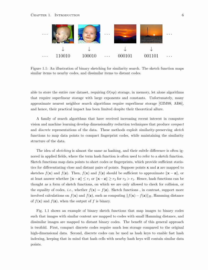
Figure 1.1: An illustration of binary sketching for similarity search. The sketch function mapssimilar items to nearby codes, and dissimilar items to distant codes.
able to store the entire raw dataset, requiring O(np) storage, in memory, let alone algorithms
that require superlinear storage with large exponents and constants. Unfortunately, many
approximate nearest neighbor search algorithms require superlinear storage [GIM99, AI06],
and hence, their practical impact has been limited despite their theoretical allure.
A family of search algorithms that have received increasing recent interest in computer
vision and machine learning develop dimensionality reduction techniques that produce compact
and discrete representations of the data. These methods exploit similarity-preserving sketch
functions to map data points to compact fingerprint codes, while maintaining the similarity
structure of the data.
The idea of sketching is almost the same as hashing, and their subtle difference is often ig-
nored in applied fields, where the term hash function is often used to refer to a sketch function.
Sketch functions map data points to short codes or fingerprints, which provide sufficient statis-
tics for differentiating close and distant pairs of points. Suppose points x and z are mapped to
sketches f(x) and f(z). Then, f(x) and f(z) should be sufficient to approximate ‖x − z‖, or
at least answer whether ‖x− z‖ ≤ r1 or ‖x− z‖ ≥ r2 for r2 > r1. Hence, hash functions can be
thought as a form of sketch functions, on which we are only allowed to check for collision, or
the equality of codes, i.e., whether f(x) = f(z). Sketch functions , in contrast, support more
involved calculations on f(x) and f(z), such as computing ‖f(x)− f(z)‖H , Hamming distance
of f(x) and f(z), when the output of f is binary.
Fig. 1.1 shows an example of binary sketch functions that map images to binary codes
such that images with similar content are mapped to codes with small Hamming distance, and
dissimilar images are mapped to distant binary codes. The benefit of this general approach
is twofold. First, compact discrete codes require much less storage compared to the original
high-dimensional data. Second, discrete codes can be used as hash keys to enable fast hash
indexing, keeping that in mind that hash cells with nearby hash keys will contain similar data
points.

Chapter 1. Introduction 7
Similar data points:
‖h− g‖H
`hinge(h,g, 1)
ρ−1
Dissimilar data points:
‖h− g‖H
`hinge(h,g, 0)
ρ+1
Figure 1.2: Visualization of pairwise hinge loss for learning binary hash (sketch) functions.
1.5 Our approach to learning hash functions
In this thesis, we advocate the use of compact binary codes for scalable similarity search. We
discuss three ways of learning binary sketch functions from data in Chapters 2, 3, and 5. In the
reminder of thesis, we use the term hash function to refer to a sketch function in order to be
consistent with the literature that does not differentiate sketching and hashing [SVD03, SH09,
TFW08, KD09].
In Chapter 2, we propose a method for learning binary linear threshold functions that map
high dimensional data onto binary codes. Our formulation is based on structured prediction
with latent variables and a pairwise hinge loss function. We assume that training data is
organized into pairs of similar and dissimilar points, which should be mapped to codes that
preserve the similarity labels. Given a hyper-parameter ρ, binary codes h and g are considered
similar if their Hamming distance is smaller than ρ, i.e., ‖h− g‖H ≤ ρ− 1. Conversely, codes
h and g are considered dissimilar if ‖h−g‖H ≥ ρ+ 1. We use a pairwise hinge loss depicted in
Fig. 1.2 to optimize the parameters of hash function for pairs of similar and dissimilar training
data points. The proposed learning algorithm is efficient to train for large datasets, scales well
to large code lengths, and outperforms state-of-the-art methods.
For some tasks and datasets, classifying the training data into similar vs. dissimilar pairs is
nearly impossible. Moreover, compared to more advanced projections by multilayer neural net-
works, linear threshold functions are limited in their expressive power. We address both of these
concerns by presenting a framework for learning a broad family of non-linear mapping functions
using a flexible form of triplet ranking loss. The training dataset D, as shown in Fig. 1.3, is
organized into triplets of exemplars, D ={
(xi,x+i ,x
−i )}ni=1
, such that xi is more similar to x+i
than x−i . We define a triplet ranking loss function that penalizes a triplet of binary codes when
Hamming distance between the more similar pair is larger than Hamming distance between the
D ={(
, ,),(
, ,), . . .
}Figure 1.3: An illustration of training data organized into triplets, D =
{(xi,x
+i ,x
−i )}ni=1
, such
that xi is more similar to x+i than x−i .

Chapter 1. Introduction 8
Figure 1.4: Illustration of Hamming ball with a radius of r bits in the vicinity a code 0000.
less similar pair. Employing this loss function, we aim to learn hash functions that satisfy as
many triplet ranking constraints as possible. We overcome the discontinuous optimization of
the discrete mapping by minimizing a piecewise smooth upper bound on empirical loss. A new
loss-augmented inference algorithm that is quadratic in the code length is proposed. We use
stochastic gradient descent for scalable optimization.
1.6 Search in Hamming space
There has been growing interest in representing image data and feature descriptors in terms
of compact binary codes, often to facilitate fast near neighbor search and feature matching
in vision applications (e.g., [AOV12, CLSF10, SVD03, SBBF12, TFW08, KGF12]). Nearest
neighbor search (NNS) on binary codes is used for image search [RL09, TFW08, WTF08],
matching local features [AOV12, CLSF10, JDS08, SBBF12], image classification [BTF11a], etc.
Sometimes the binary codes are generated directly as feature descriptors for images or image
patches, such as BRIEF or FREAK [CLSF10, BTF11a, AOV12, TCFL12], and sometimes
binary corpora are generated by similarity-preserving hash functions from high-dimensional
data, as discussed above. Regardless of the algorithm used to generate the binary codes, one
has to develop algorithms for search in Hamming space that scale to massive datasets.
To facilitate NNS in Hamming space previous work suggests creating hash tables on the
binary codes in the dataset, and retrieving the contents of the hash buckets in the vicinity of a
query code to find near neighbors. The problem is that the number of hash buckets within a
Hamming ball around a query, which one might have to examine in order to find near neighbors
(see Fig. 1.4), grows near-exponentially with the search radius. When binary codes are longer
than 64 bits, even with a small search radius, the number of buckets to examine may be larger
than the number of items in the database, hence slower than linear scan.
In Chapter 4 of the thesis, inspired by the work of Greene, Parnas, and Yao [GPY94],
we introduce a rigorous way to build multiple hash tables on binary code substrings to enable
exact k-nearest neighbor search in Hamming distance. Our approach, called multi-index hashing
(MIH), is storage efficient and straight-forward to implement. We present theoretical analysis

Chapter 1. Introduction 9
that shows that the algorithm exhibits sublinear run-time behavior for uniformly distributed
codes. In addition, our empirical with non-uniformly distributed codes show dramatic speedups
over a linear scan baseline for datasets of up to one billion codes of 64, 128, or 256 bits.
The algorithm for searching binary codes complements the methods for learning binary hash
functions to build a full system for large-scale similarity search.
1.7 Vector quantization for nearest neighbor search
Sketch functions map data points to short codes that provide sufficient statistics to differentiate
close and distant pairs of points. Vector quantizers map data points to compressed codes
sufficient to approximately reconstruct the original data. They can be thought as a form of
sketch functions too. Let f(x) denote the quantization of x, and suppose x can be reconstructed
by f−1(f(x)). Then, we can compute the distance between x and z by simply computing
‖f−1(f(x))−f−1(f(z))‖. The benefit is that we are no longer required to keep high-dimensional
vectors x and z in memory, but only having access to compressed codes f(x) and f(z) suffices
to estimate ‖x − z‖. For this approach to be effective, we expect estimation of distance given
f(x) and f(z) to be faster than simply computing ‖x− z‖, so we are interested in a sub-family
of vector quantizers that allow fast distance estimation.
As an example, consider quantization by mapping data points to their k-means cluster
centers. Given a set of k centers denoted {C(i)}ki=1, the quantizer f(x) is defined as:
f(x) = argmini‖x− C(i)‖22 . (1.2)
One can approximate Euclidean distance ‖x − z‖22 by the distance between cluster centers
associated with x and z, i.e., ‖C(f(x))−C(f(z))‖22. Pairwise distances between cluster centers
can be precomputed and stored in a lookup table to provide a fast way for distance estimation.
One way to reduce the error in distance estimation is to only quantize the database points
and not the query [JDS11]. This way, one can approximate distance between x and z by
‖C(f(x)) − z‖22. For each query z, a query-specific lookup table can be created that stores
the distance between z and all of the k cluster centers. As long as k is much smaller than n,
creating the lookup table for distance estimation with k-means is effective.
We note that vector quantizers can be used for hashing as well as distance estimation.
When used for hashing, as described in Section 1.3, all of the data points sharing the same
quantization code are mapped to a hash bucket, which can be accessed by a query look up
efficiently. In this case, we need to keep the number of quantization regions small, roughly
in the range of n, so we do not allocate many hash buckets that are empty. However, when
quantization is used for distance estimation, in order to reduce the estimation error we need
to increase the number of quantization regions, so long as the memory footprint is acceptable.
This has led to hybrid approaches to Euclidean NNS [JDS11, BL12]: A coarse quantization of
Chapter 1. Introduction 10
the space is used with hashing to reduce the search problem to a reasonable short list of near
neighbor candidates. A fine quantization of the space is used for distance estimation to rank
the short list candidates and find the nearest neighbors. The fine quantization allows one to
save memory by discarding the original high-dimensional vectors, if only keeping the quantized
vectors yields sufficiently good approximate results.
For the quantization approach to be useful for distance estimation, we need small vector
quantization errors that yield small error in distance estimation. Increasing the number of
cluster centers in k-means is one way to reduce quantization error, but vector quantization
with k-means is slow and memory intensive especially when k gets large. In this thesis, we
develop new models related to k-means clustering with a compositional parametrization of
cluster centers, so representational capacity and effective number of quantization regions in-
crease super-linearly in the number of parameters. This allows one to efficiently quantize data
using billions or trillions of centers. We formulate two such models, Orthogonal k-means and
Cartesian k-means. They are closely related to one another, to k-means, to methods for binary
hash function optimization like ITQ [GL11], and to Product Quantization for vector quanti-
zation [JDS11]. With the help of these techniques one can devise fast and memory efficient
models for Euclidean NNS.
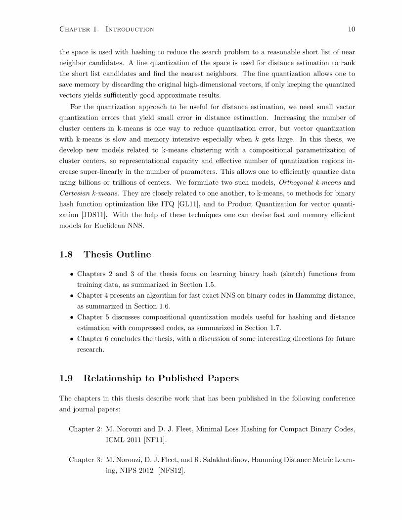
1.8 Thesis Outline
• Chapters 2 and 3 of the thesis focus on learning binary hash (sketch) functions from
training data, as summarized in Section 1.5.
• Chapter 4 presents an algorithm for fast exact NNS on binary codes in Hamming distance,
as summarized in Section 1.6.
• Chapter 5 discusses compositional quantization models useful for hashing and distance
estimation with compressed codes, as summarized in Section 1.7.
• Chapter 6 concludes the thesis, with a discussion of some interesting directions for future
research.
1.9 Relationship to Published Papers
The chapters in this thesis describe work that has been published in the following conference
and journal papers:
Chapter 2: M. Norouzi and D. J. Fleet, Minimal Loss Hashing for Compact Binary Codes,
ICML 2011 [NF11].
Chapter 3: M. Norouzi, D. J. Fleet, and R. Salakhutdinov, Hamming Distance Metric Learn-
ing, NIPS 2012 [NFS12].

Chapter 1. Introduction 11
Chapter 4: M. Norouzi, A. Punjani, and D. J. Fleet, Fast Search in Hamming Space with
Multi-Index Hashing, CVPR 2012 [NPF12].
M. Norouzi, A. Punjani, and D. J. Fleet, Fast Exact Search in Hamming Space
with Multi-Index Hashing, TPAMI 2014 [NPF14].
Chapter 5: M. Norouzi, D. J. Fleet, Cartesian k-means, CVPR 2013 [NF13].

Chapter 2
Minimal Loss Hashing
A common approach to approximate nearest neighbor search, well suited to high-dimensional
data, uses similarity-preserving hash functions, where similar/dissimilar pairs of inputs are
mapped to nearby/distant hash codes. One can preserve Euclidean distances, e.g., with Locality-
Sensitive Hashing (LSH) [IM98], or one might want to preserve the similarity associated with
object category labels, or real-valued affinities associated with training exemplars.
Using compact binary codes as hash keys is particularly useful for nearest neighbor search
(NNS). If the neighbors of a query fall within a small Hamming ball in Hamming space, then
search can be accomplished in sublinear time, by enumerating over all of the binary hash codes
within the Hamming ball in the vicinity of the query code. Even an exhaustive linear scan
through the database of binary codes enables very fast search. Moreover, compact binary codes
allow one to store large databases in memory.
Finding a suitable mapping of the data onto binary codes has a profound impact on the
quality of a hashing-based NNS system. Random projections are used in LSH [IM98, Cha02] and
related methods [RL09, Bro97]. They are dataset independent, make no prior assumption about
the data distribution, and come with theoretical guarantees that specific metrics (e.g., cosine
similarity) are increasingly well preserved in Hamming space as the code length increases. But
they require large code lengths for good retrieval accuracy, and they are not applicable to
general similarity measures, like human ratings.
To find better more compact codes, recent research has turned to machine learning tech-
niques that optimize mappings for specific datasets (e.g., [KD09, SH09, SVD03, TFW08,
BTF11b]). Most learning methods aim to preserve Euclidean structure of the input datasets
(e.g., [GL11, KD09, WTF08]). However, some papers also considered more generic measures
of similarity. Unsupervised multilayer neural nets of Salakhutdinov and Hinton [SH09] aim
to discover semantic similarity using deep autoencoders with stochastic binary code layers.
Shakhnarovich, Viola, and Darrel [SVD03] exploit boosting to learn binary hash bits greedily
from supervised similarity labels. By contrast, the method that we propose in this chapter is
supervised and not sequential; it optimizes all the code bits simultaneously.
The task at hand is to find a hash function that maps high-dimensional inputs, x ∈ Rp,
12

Chapter 2. Minimal Loss Hashing 13
onto q-bit binary codes, h ∈ Hq ≡ {−1, 1}q, which preserves some notion of similarity. The
canonical approach assumes centered (mean-subtracted) inputs, linear projection, and binary
quantization. Such hash functions, parameterized by W ∈ Rq×p, are given by
b lin(x;w) = sign (Wx), (2.1)
where w≡vec(W ), and the ith bit of the vector sign(Wx) is 1 iff the ith dimension of (Wx) is
positive. In other words, the ith row of W determines the ith bit of the hash function in terms
of a hyperplane in the input space; −1 is assigned to points on one side of the hyperplane, and
1 to points on the other side.1
The main difficulty in optimizing similarity-preserving binary hash functions stems from
the discontinuity of the projection, resluting in a discontinuous learning objective function.
At a high level, there exist at least three general ways to minimize a discontinous objective.
First, coordinate descent where one iteratively optimizes each parameter dimention separately
by exhaustive enumeration a large collection of possible values (e.g., see [KD09]). Second,
continuous relaxations where one approximates b lin(x;w) by a smooth function such as tangent
hyperbolic. Third, optimization via a continous upper bound on the discontinuous objective,
which is the approach that we follow in this work.
In this chapter, we formulate the learning of compact binary codes in terms of structured
prediction with latent variables using new classes of loss functions designed for preserving
similarity. We design a loss function specifically for hashing that takes Hamming distance
and binary quantization into account. Our novel formulation adopts the approach of latent
structural SVMs [YJ09] and an effective online learning algorithm. The resulting algorithm is
shown to outperform state-of-the-art methods.
2.1 Formulation
Turning to formulation, let a training dataset D comprise n pairs of p-dimensional training
points (xi,x′i) along with their similarity label si ∈ {0, 1}, i.e., D ≡ {(xi,x′i, si)}
ni=1. The data
points xi and x′i are similar when the binary similarity label is 1 (si = 1), and dissimilar when
si = 0. To preserve a specific metric (e.g., Euclidean distance) one can use binary similarity
labels obtained by thresholding pairwise distances. Alternatively, for preserving similarity based
on semantic content of examples, one can use a weakly supervised dataset in which each training
point is associated with a set of neighbors (similar exemplars), e.g., with the same class label,
and non-neighbors (dissimilar exemplars), e.g., with different class labels.
The quality of a mapping b lin(x;w) is determined by a loss function `pair : Hq×Hq×{0, 1} →R+ that assigns a cost to a pair of binary codes and a similarity label. For binary codes h ∈ Hq,
g ∈ Hq, and a label s ∈ {0, 1}, the loss function `pair(h,g, s) measures how compatible h and
1One can add an offset from the origin, but we find the gain is marginal. Nonlinear projections are alsopossible, but in this chapter we concentrate on linear projections.

Chapter 2. Minimal Loss Hashing 14
g are with s. For example, when s = 1, the loss assigns a small cost if h and g are nearby
codes, and large cost otherwise. Ultimately, to learn w, we aim to minimize empirical loss over
training pairs:
L(w) =
n∑i=1
`pair(b(xi;w), b(x′i;w), si) . (2.2)
2.1.1 Pairwise hinge loss
The loss function that we advocate is specific to learning binary hash functions, and bears strong
similarity to hinge loss used in SVMs. It includes a hyper-parameter ρ, which is a threshold
in the Hamming space that differentiates neighbors from non-neighbors. This is important for
learning hash codes, since we want similar training points to map to binary codes that differ
by no more that ρ bits. Non-neighbors should map to codes no closer than ρ bits.
Let ‖h − g‖H denote Hamming distance between binary codes h and g. Our hinge loss
function, denoted `hinge, depends on ‖h− g‖H and not on the individual codes:
`hinge(h,g, s) =
[‖h− g‖H − ρ+ 1
]+
for s = 1
λ[ρ− ‖h− g‖H + 1
]+
for s = 0
(2.3)
where [α]+ ≡ max(α, 0), and λ is another loss hyper-parameter that controls the ratio of the
slopes of the penalties incurred for similar vs. dissimilar points when they are too far apart
vs. too close. Linear penalties are useful as they are robust to outliers. Note that when similar
points are sufficiently close, or dissimilar points are distant, our loss does not impose any
penalty. The `hinge(h,g, s) loss is depicted in Fig. 1.2.
2.1.2 Binary Reconstructive Embedding
Our loss-based framework for learning binary hash functions is inspired by Binary Eeconstruc-
tive Embedding (BRE) introduced by Kulis and Darrel [KD09]. The BRE uses a different
pairwise loss function that penalizes the squared difference between normalized Hamming dis-
tance in binary codes and a real-valued distance in the input space. Given two q-bit codes h
and g for data points x and x′, and a parameter 0 ≤ d ≤ 1 which represents a measure of
distance between x and x′, the BRE loss takes the form of
`bre(h,g, d) =
(( 1
q‖h− g‖H
)2 − d2)2
. (2.4)
The BRE [KD09] assumes that inputs are unit norm, and uses d = 12‖x−x
′‖2. This is equivalent
to d = 1− cos(θ(x,x′)) for unnormalized x and x′, which makes `bre loss particularly suitable
for preserving cosine similarity, and relates BRE to angular LSH [Cha02]. That said, other
normalized distance measures (between 0 and 1) can be used within the BRE loss too to define
Chapter 2. Minimal Loss Hashing 15
the value of d, for instance d = 1− s.The BRE method [KD09] addresses the difficulty in optimizing empirical loss in (2.2) by
using coordinate descent. At each iteration of the optimzation, the BRE adjusts one entry of
W by exhaustive search. By changing a single entry of W , denoted W[a,b], only one bit in the
output binary codes can change (i.e., ath bit). For each training data point, one can compute
the value of W[a,b] that flips the ath bit of the code for that data point. Therefore a set of n
thresholds are computed, one for each training point, and the optimal threshold is selected as
the new value of W[a,b] by exhaustive evaluation of empirical loss for all thresholds. During
training, to enable faster parameter update, the BRE caches q-dimensional real-valued linear
projections of the training data points. This incurs high storage cost for training, making large
datasets impractical.
In the BRE optimization, coordinate descent is possible because of the restricted form of the
hash functions b lin(.). For a more general family of hash functions e.g., based on thresholded
multilayer neural networks, coordiante descent is not possible anymore as changing one entry
in the weights from −∞ to +∞ may flip multiple bits in the output codes several times. By
contrast, the approach that we propose in this section can be applied to both b lin(.) and a more
general family of hash functions, discussed in Section 3.
2.2 Bound on empirical loss
The empirical loss in (2.2) is discontinuous and typically non-convex, making optimization
difficult. Rather than directly minimizing empirical loss, we instead formulate, and minimize,
a piecewise linear upper bound on empirical loss. Our bound is inspired by a bound used, for
similar reasons, in latent structural SVMs [YJ09].
We first re-express the hash function b lin(x;w) as a form of structured prediction:
b lin(x;w) = sign (Wx), (2.5a)
= argmaxh∈Hq
hTWx (2.5b)
= argmaxh∈Hq
wTψ(x,h) , (2.5c)
where ψ(x,h) ≡ vec(hxT). Here, wTψ(x,h) acts as a scoring function that determines the
relevance of input-output pairs, based on a weighted sum of features in their joint feature
vector ψ(x,h). Note that other forms of ψ(x,h) are possible too, leading to other types of hash
functions. For example one may consider pairwise weights for interactions between binary bits
within h which would require a binary quadratic optimization for inference. That said, this
chapter focuses on the simplest family of hash functions based on linear threshold functions.
To motivate our upper bound on empirical loss, we begin with a short review of the bound
commonly used for structural SVMs [TGK03, THJA04].

Chapter 2. Minimal Loss Hashing 16
2.2.1 Structural SVM
In structural SVMs, given input-output training pairs {(xi,y∗i )}ni=1, one aims to learn a mapping
from inputs to discrete outputs in terms of a parameterized scoring function f(x,y;w), such
that the model’s prediction y,
y = argmaxy
f(x,y;w) , (2.6)
correlates closely with the ground-truth label y∗. Given a loss function on the output domain,
`(·, ·), the structural SVM with margin-rescaling introduces a margin violation (slack) variable
for each training pair, and minimizes sum of slack variables. For a pair (x, y∗), slack is defined
as
maxy
[`(y,y∗)+f(x,y;w)]− f(x,y∗;w) . (2.7)
Importantly, the slack variables provide an upper bound on loss for the model’s prediction y :
`(y,y∗)
≤ maxy
[`(y,y∗)+f(x,y;w)]− f(x, y;w) (2.8a)
≤ maxy
[`(y,y∗) + f(x,y;w)]− f(x,y∗;w) . (2.8b)
To see the inequality in (2.8a), note that, if the first term on the RHS of (2.8a) is maximized by
y = y, then the f terms cancel, and (2.8a) becomes an equality. Otherwise, the optimal value
of the max term must be larger than when y = y, which causes the inequality. The second
inequality (2.8b) follows straightforwardly from the definition of y in (2.6); i.e., f(x, y;w) ≥f(x,y;w) for all y including y∗. The bound in (2.8b) is piecewise linear, convex in w, and easier
to optimize than the empirical loss. Structural SVM formulates learning as the minimization
of the sum of bounds in (2.8b) for every training examples (i.e., sum of slack variables), plus a
regularizer on w.
2.2.2 Convex-concave bound for hashing
The difference between learning hash functions and the structural SVM is that the binary codes
for our training data are not known a priori. However, note that the tighter bound in (2.8a)
uses y∗ only in the loss term. This is useful for hash function learning, as suitable loss functions
for hashing, such as `bre and `hinge, do not require ground-truth labels, but a pair of binary
codes. The bound (2.8a) is piecewise linear, convex-concave (a sum of convex and concave
terms), and is the basis for structural SVMs with latent variables [YJ09]. Below we formulate
a similar bound for learning binary hash functions.
Our upper bound on a generic pairwise loss function `pair, given a pair of inputs, x and x′,

Chapter 2. Minimal Loss Hashing 17
a similarity label s, and the parameters of the hash function w, has the form
`pair( b lin(x;w), b lin(x′;w), s)
≤ maxg,g′∈Hq
{`pair(g,g
′, s) + gTWx + g′TWx′
}− max
h∈HqhTWx− max
h′∈Hqh′
TWx′ .
(2.9)
It follows from the definition of b lin(.) that the second and third terms on the RHS of (2.9)
are maximized by h = b lin(x;w) and h′ = b lin(x′;w). If the first term were maximized by
g = b lin(x;w) and g′ = b lin(x′;w), then the inequality in (2.9) becomes an equality. For all
other values of g and g′ that maximize the first term, the RHS can only increase, hence the
inequality. The bound holds for any loss function `pair including `bre and `hinge.
We formulate the optimization for learning the weights w of the hashing function, in terms
of minimization of the following convex-concave upper bound on empirical loss:
n∑i=1
(maxgi,g′i
{`pair(gi,g
′i, si) + gi
TWxi + g′iTWx′i
}−max
hi
hiTWxi −max
h′i
h′iTWx′i
). (2.10)
2.2.3 Tightness of the bound and regularization
Regarding the tightness of the bound in (2.9), we present a proposition that helps understanding
the nature of empirical loss optimization via minimizing the upper bound. Clearly, the loss
`pair(b lin(x;w), b lin(x′;w), s) does not change with the norm of w as b lin(x;w) = b lin(x;αw)
for any scalar α > 0. However, change in the norm of w affects the upper bound in (2.9). We
claim that the upper bound gets tighter as the norm of w gets larger. In other words, the
bound for γw for any γ > 1 is smaller than or equal to the bound for w:
maxg,g′∈Hq
{`pair(g,g
′, s) + γgTWx + γg′TWx′
}− max
h∈HqγhTWx− max
h′∈Hqγh′
TWx′
≤ maxg,g′∈Hq
{`pair(g,g
′, s) + gTWx + g′TWx′
}− max
h∈HqhTWx− max
h′∈Hqh′
TWx′ .
(2.11)
We provide an algebraic proof of (2.11) in Section 2.A.
Given the proposition (2.11), one undesirable way to minimize the upper bound is to increase
the norm of w, which does not affect the loss, but the bound. In particular, when γ goes to
+∞, it is easy to see that the upper bound and the actual loss become equivalent as the score
terms dominate the maximization over g and g′ (unless Wx and Wx′ are zero). Hence, when
‖w‖ is really large, the upper bound becomes really tight and almost piecewise constant in
w, so using the gradient of the bound for optimization with respect to w is hopeless. On the
other hand, when γ goes to zero, the score terms will not affect the maximization over g and
g′, and all of the terms except loss go to zero, so the upper bound becomes a constant value of
maxg,g′ {`pair(g,g′, s)}.
Chapter 2. Minimal Loss Hashing 18
To prevent w from growing really large during optimization, we use a regularizer on ‖w‖22.According to our experiments, using a regularizer on w leads to a smaller value of emprical
loss after convergence. We believe that constraining the norm of w makes the upper bound
looser, but also makes the bound smoother, leading to more progress by the gradient based
optimizer. Because the bound is non-convex, gradient based optimization is one of the only
options available. The regularizer that we choose for optimization of b lin, is a set of hard
constraints on the `2 norm of rows of W . This way we have control over the norm of each
hyperplane separately.
Including a regularizer, here is the surrogate objective that we aim to minimize given a
training dataset of n similar / dissimilar pairs of data points (xi,x′i) and their labels si:
n∑i=1
(maxgi,g′i
{`pair(gi,g
′i, si) + gi
TWxi + g′iTWx′i
}−max
hi
{hi
TWxi}−max
h′i
{h′i
TWx′i
}) s. t. ∀1≤ j≤ q∥∥W[j, ·]
∥∥22≤ ν , (2.12)
where ν is a hyper parameter controlling the regularization, and W[j, ·] is the jth row of W .
2.3 Optimization
Minimizing (2.12) to find w entails the maximization of three terms for each training pair
(xi,x′i). The second and third terms are trivially maximized directly by the hash function
itself. Maximizing the first term is, however, not trivial. In the structural SVM literature,
optimizing this term is called loss-augmented inference. The next section describes an efficient
algorithm for finding the exact solution of loss-augmented inference for hash function learning
with pairwise losses.
2.3.1 Loss-augmented inference with pairwise hashing loss
To solve loss-augmented inference, one needs to find a pair of binary codes g and g′ given by
(g, g′) = argmax(g,g′)∈Hq×Hq
{`pair(g,g
′, s) + gTWx + g′TWx′
}. (2.13)
We solve loss-augmented inference exactly and efficiently for loss functions of the form
`pair(g,g′, s) = `
(‖g − g′‖H , s
), (2.14)
such as `hinge and `bre that depend on Hamming distance between g and g′ but not the specific
bit sequences g and g′. Before deriving a general solution, first consider a specific case for
which we restrict the Hamming distance between g and g′ to be m, i.e., ‖g − g′‖H = m. For
q-bit codes, m is an integer between 0 and q. When ‖g− g′‖H = m, the loss in (2.13) depends

Chapter 2. Minimal Loss Hashing 19
on m and s, but not on g or g′. Thus, instead of (2.13), we can now solve
`(m, s) + maxg,g′
{gTWx + g′
TWx′
}s. t. ‖g − g′‖H = m . (2.15)
The key to finding the two codes that maximize (2.15) is to decide which m bits in the two
codes should be different.
Let v[k] denote the kth dimension of a vector v. We can compute the joint contribution of
the kth bits of g and g′ to(gTWx + gTWx′
)by
cont(k,g[k],g′[k]) = g[k](Wx)[k] + g′[k](Wx′)[k] , (2.16)
and these contributions can be computed for the four possible states of the kth bits. Let δk
represent how much is gained by setting the bits g[k] and g′[k] to be different rather than the
same, i.e.,
δk = max(cont(k, 1,−1), cont(k,−1, 1)
)−max
(cont(k,−1,−1), cont(k, 1, 1)
)(2.17)
Because g and g′ differ only in m bits, optimal g and g′ are obtained by setting the m bits with
m largest δk’s to be different. All other bits in the two codes should be the same. When g[k] and
g′[k] must be different, their best values are found by comparing cont(k, 1,−1) and cont(k,−1, 1).
Otherwise, they are determined by the larger of cont(k,−1,−1) and cont(k, 1, 1). Now solve
(2.15) for all m; noting that we only compute δk for each bit once.
In sum, to solve the loss-augmented inference it suffices to find the m that provides the
largest value for the objective function in (2.15). We first sort the δk’s once, and for different
values of m, we compare the sum of the first m largest δk’s plus `(m, s), and choose the m that
achieves the highest score. Afterwards, we determine the values of the bits according to their
contributions as described above.
Given the values of Wx and Wx′, this loss-augmented inference algorithm takes time
O(q log q). Other than sorting the δk’s, all other steps are linear in q which makes the in-
ference efficient and scalable to large code lengths. The computation of Wx can be done once
per data point and cached, in case the data point is being used in multiple pairs.
2.3.2 Perceptron-like learning with pairwise loss
In Section 2.2.3, we formulated a convex-concave bound in (2.12) on empirical loss, which we
use as a surrogate objective for learning binary hash functions. In Section 2.3.1 we described
how the value of the bound could be computed at a given W for a given (xi,x′i, si). Now
we consider optimizing the objective i.e., lowering the bound. A standard technique for mini-
mizing such objectives is called difference of convex (DC) programming or the concave-convex
procedure [YR03]. Applying this method to our problem, we should iteratively impute the
missing data (the binary codes b lin(xi) and b lin(x′i)) and optimize for the convex term (the loss-

Chapter 2. Minimal Loss Hashing 20
200 400 600 800 1000 1200 1400 1600 1800 200050
100
150
Iterations
Valu
e s
um
med o
ver
105
pairs
Upperbound
Empirical loss
Figure 2.1: The upper bound and empirical loss as functions of optimization step.
augmented terms in (2.12)). However, our preliminary experiments showed that convex-concave
procedure is slow and not so effective for our optimization problem.
Alternatively, inspired by structured perceptron [Col02] and McAllester et al. [MHK10],
we employ a stochastic gradient-based approach based on an iterative perceptron-like update
rule. At iteration t of optimization, let the current weight matrix be W (t). Then, we randomly
sample a training pair (xt,x′t) with a similarity label st, and compute,
ht = sign(W (t)xt
)(2.18a)
h′t = sign(W (t)x′t
)(2.18b)
(gt, g′t) = argmax(g,g′)∈Hq×Hq
{`pair(g,g
′, st) + gTW (t)xt + g′TW (t)x′t
}. (2.18c)
Next, we update the parameters according to the following simple learning rule:
W (t+1) ←W (t) − η(gtxt
T + g′tx′tT − htxt
T − h′tx′tT), (2.19)
where η is the learning rate, and we project rows of W whose `2 norm exceeds ν back into the
feasible set,
For j = 1 to q : if∥∥∥W (t+1)
[j, ·]
∥∥∥22> ν, then W
(t+1)[j, ·] ←
√ν ·W (t+1)
[j, ·]∥∥∥W (t+1)[j, ·]
∥∥∥2
. (2.20)
The update rule of (2.19) follows the noisy gradient descent direction of our convex-concave
objective in (2.12). To see this, note that ∂hTWx/∂W = xhT. However, also note that the
objective in (2.12) is piecewise smooth, due to the max operations, and thus not differentiable
at isolated points. Hence, the gradient is not defined at such points, and since the objective
is not convex, sub-gradient methods are not applicable. Thus, it is difficult apply standard
convergence proofs to this learning rule. While the theoretical properties of this learning al-
gorithm needs further investigation (e.g., see [MHK10]), we empirically verify that the update
rule lowers the upper bound, and converges to a local minima. Fig. 2.1 plots the empirical loss
and the bound, computed over 105 training pairs, as a function of the iteration number.

Chapter 2. Minimal Loss Hashing 21
2.4 Implementation details
To optimize (2.12) as a means of learning hash functions, one needs to select an appropriate ν to
constrain the norms of rows of W as much as needed. In our experiments, we set ν = 1, but we
introduce another parameter, denoted ε, with identical effects. The parameter ε is multiplied
by the value of the loss to obtain the following objective function,
n∑i=1
(maxgi,g′i
{ε · `pair(gi,g′i, si) + gi
TWxi + g′iTWx′i
}−max
hi
{hi
TWxi}−max
h′i
{h′i
TWx′i
}) s. t. ∀1≤ j≤ q∥∥W[j, ·]
∥∥22≤ 1 .
(2.21)
One can verify that given a pair of (W , ν) from (2.12), W ′ = W/√ν satisfies the constrains in
(2.21) and ε = 1/√ν provides an identical behavior of the objective function. We select ε by
validation on a set of candiate choices. The benefit of using ε, instead of ν, is that for different
ε the range of W can stay the same, and similar learning rates can be used.
We initialize W using angular LSH [Cha02]; i.e., the entries of W are sampled i.i.d. from
a standard normal density N (0, 1), and each row is then normalized to have unit length. This
initialization is particularly well suited for preservation of cosine similarity.
The learning rule in (2.19) is used with several minor modifications: 1) In loss-augmented
inference (2.13), the loss is multiplied by ε. 2) We use mini-batches of size 100 to compute the
gradient. 3) We use a momentum term, which adds the gradient of the previous step with a
ratio of 0.9 to the current gradient.
For each experiment, we select 10% of the training set as a validation set. We choose the
loss hyper-parameters ρ and λ by validation on a few candidate choices. We allow the candidate
choices for ρ to linearly increase with the code length. Each epoch includes a random sample of
105 data point pairs, independent of the mini-batch size or the number of training points. For
validation, we optimize parameteres using 100 epochs, and for training, we use 2000 epochs.
For small datasets, a smaller number of epochs was used. Using fewer epochs for validation
vs. training is not ideal, but to accelerate the experimetns we chose to stop validation iterations
after fewer epochs. We found that even validation with fewer epochs results in very good results.
2.5 Experiments
We compare our approach, minimal loss hashing – MLH, with several state-of-the-art methods.
Results for binary reconstructive embedding; BRE [KD09], spectral hashing; SH [WTF08],
shift-invariant kernel hashing; SIKH [RL09], and multilayer neural nets with supervised fine-
tuning; NNCA [TFW08], were obtained with implementations generously provide by their
respective authors. For locality-sensitive hashing; LSH [Cha02], we used our own implemen-
tation. We show results of SIKH for experiments with larger datasets and longer code lengths

Chapter 2. Minimal Loss Hashing 22
only, because it was not competitive otherwise.
Each dataset comprises a training set, a test set, and a set of ground-truth neighbors. For
evaluation, we compute precision and recall for points retrieved within a Hamming distance
R of codes associated with the test queries. Precision as a function of R is H/T , where T
is the total number of points retrieved in Hamming ball with radius R, H is the number of
true neighbors among them. Recall as a function of R is H/G where G is the total number of
ground-truth neighbors.
2.5.1 Six datasets
We first mirror the experiments of Kulis and Darrell [KD09] with five datasets2: Photo-tourism,
a corpus of image patches represented as 128D SIFT features [SSS06]; LabelMe and Peekaboom,
collections of images represented as 512D Gist descriptors [TFW08]; MNIST, 784D greyscale
images of handwritten digits; and Nursery, 8D features. We also use a synthetic dataset
comprising uniformly sampled points from a 10D hypercube [WTF08]. Like Kulis and Darrel we
used 1000 random points for training, and 3000 points (where possible) for testing; all methods
used identical training and test sets. The neighbors of each data-point are defined with a
dataset-specific threshold. On each training set we find the Euclidean distance at which each
point has, on average, 50 neighbors. This defines ground-truth neighbors and non-neighbors for
training, and for computing precision and recall statistics during testing.
For preprocessing, each dataset is mean-centered. For all but the 10D Uniform data, we
then normalize each datum to have unit length. Because some methods (BRE, SH, SIKH)
improve with dimensionality reduction prior to training and testing, we apply PCA to each
dataset (except 10D Uniform and 8D Nursery) and retain a 40D subspace. MLH often performs
slightly better on the full datasets, but we report results for the 40D subspace, to be consistent
with the other methods.
For all methods with local minima or stochastic optimization (i.e., all but SH) we optimize
10 independent models, at each of several code lengths. Fig. 2.3 plots precision (averaged over
10 models, with standard deviation bars), for points retrieved within a Hamming radius R = 3
using difference code lengths. These results are similar to those in [KD09], where BRE yields
higher precision than SH and LSH for different binary code lengths. The plots also show that
MLH consistently yields higher precision than BRE. This behavior persists for a wide range of
retrieval radii as shown in Fig. 2.2 for Hamming radii of R = 1 and R = 5 on LabelMe.
For many retrieval tasks with large datasets, precision is more important than recall. Nev-
ertheless, for other tasks such as recognition, high recall may be desired if one wants to find the
majority of similar points to each query. To assess both recall and precision, Figures 2.4 and
2.5 plot precision-recall curves (averaged over 10 models, with standard deviation bars) for all
of the six benchmarks, and for binary codes of length 15, 30, and 45. These plots are obtained
2Kulis and Darrel treated Caltech-101 differently from the other 5 datasets, with a specific kernel, so experi-ments were not conducted on that dataset.
Chapter 2. Minimal Loss Hashing 23
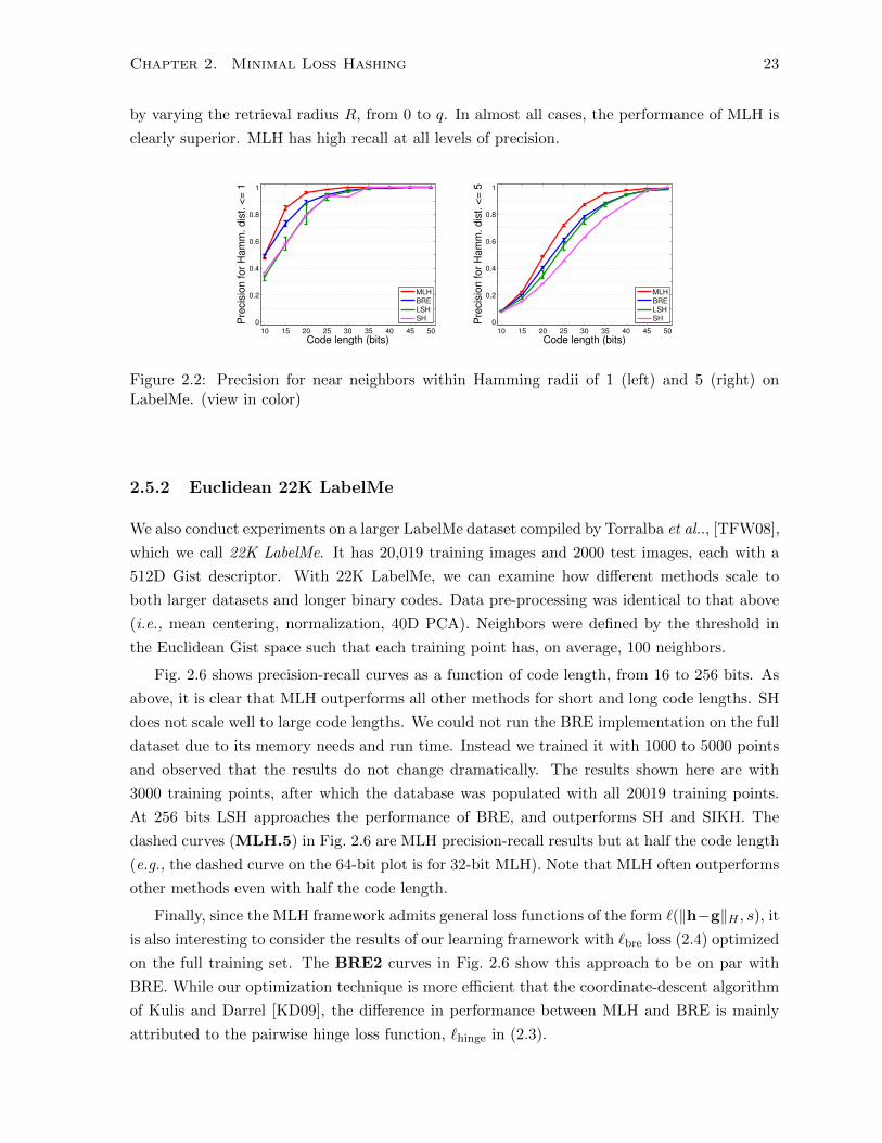
by varying the retrieval radius R, from 0 to q. In almost all cases, the performance of MLH is
clearly superior. MLH has high recall at all levels of precision.
10 15 20 25 30 35 40 45 50 0
0.2
0.4
0.6
0.8
1
Code length (bits)
Pre
cis
ion for
Ham
m. dis
t. <
= 1
MLH
BRE
LSH
SH
10 15 20 25 30 35 40 45 50 0
0.2
0.4
0.6
0.8
1
Code length (bits)
Pre
cis
ion for
Ham
m. dis
t. <
= 5
MLH
BRE
LSH
SH
Figure 2.2: Precision for near neighbors within Hamming radii of 1 (left) and 5 (right) onLabelMe. (view in color)
2.5.2 Euclidean 22K LabelMe
We also conduct experiments on a larger LabelMe dataset compiled by Torralba et al.., [TFW08],
which we call 22K LabelMe. It has 20,019 training images and 2000 test images, each with a
512D Gist descriptor. With 22K LabelMe, we can examine how different methods scale to
both larger datasets and longer binary codes. Data pre-processing was identical to that above
(i.e., mean centering, normalization, 40D PCA). Neighbors were defined by the threshold in
the Euclidean Gist space such that each training point has, on average, 100 neighbors.
Fig. 2.6 shows precision-recall curves as a function of code length, from 16 to 256 bits. As
above, it is clear that MLH outperforms all other methods for short and long code lengths. SH
does not scale well to large code lengths. We could not run the BRE implementation on the full
dataset due to its memory needs and run time. Instead we trained it with 1000 to 5000 points
and observed that the results do not change dramatically. The results shown here are with
3000 training points, after which the database was populated with all 20019 training points.
At 256 bits LSH approaches the performance of BRE, and outperforms SH and SIKH. The
dashed curves (MLH.5) in Fig. 2.6 are MLH precision-recall results but at half the code length
(e.g., the dashed curve on the 64-bit plot is for 32-bit MLH). Note that MLH often outperforms
other methods even with half the code length.
Finally, since the MLH framework admits general loss functions of the form `(‖h−g‖H , s), it
is also interesting to consider the results of our learning framework with `bre loss (2.4) optimized
on the full training set. The BRE2 curves in Fig. 2.6 show this approach to be on par with
BRE. While our optimization technique is more efficient that the coordinate-descent algorithm
of Kulis and Darrel [KD09], the difference in performance between MLH and BRE is mainly
attributed to the pairwise hinge loss function, `hinge in (2.3).
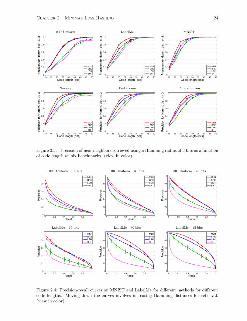
Chapter 2. Minimal Loss Hashing 24
10D Uniform LabelMe MNIST
10 15 20 25 30 35 40 45 50 0
0.2
0.4
0.6
0.8
1
Code length (bits)
Pre
cis
ion for
Ham
m. dis
t. <
= 3
MLH
BRE
LSH
SH
10 15 20 25 30 35 40 45 50 0
0.2
0.4
0.6
0.8
1
Code length (bits)
Pre
cis
ion for
Ham
m. dis
t. <
= 3
MLH
BRE
LSH
SH
10 15 20 25 30 35 40 45 50 0
0.2
0.4
0.6
0.8
1
Code length (bits)
Pre
cis
ion for
Ham
m. dis
t. <
= 3
MLH
BRE
LSH
SH
Nursery Peekaboom Photo-tourism
10 15 20 25 30 35 40 45 50 0
0.2
0.4
0.6
0.8
1
Code length (bits)
Pre
cis
ion for
Ham
m. dis
t. <
= 3
MLH
BRE
LSH
SH
10 15 20 25 30 35 40 45 50 0
0.2
0.4
0.6
0.8
1
Code length (bits)
Pre
cis
ion for
Ham
m. dis
t. <
= 3
MLH
BRE
LSH
SH
10 15 20 25 30 35 40 45 50 0
0.2
0.4
0.6
0.8
1
Code length (bits)
Pre
cis
ion for
Ham
m. dis
t. <
= 3
MLH
BRE
LSH
SH
Figure 2.3: Precision of near neighbors retrieved using a Hamming radius of 3 bits as a functionof code length on six benchmarks. (view in color)
10D Uniform – 15 bits 10D Uniform – 30 bits 10D Uniform – 45 bits
0 0.2 0.4 0.6 0.8 1
0
0.2
0.4
0.6
0.8
1
Recall
Pre
cis
ion
MLH
BRE
LSH
SH
0 0.2 0.4 0.6 0.8 1
0
0.2
0.4
0.6
0.8
1
Recall
Pre
cis
ion
MLH
BRE
LSH
SH
0 0.2 0.4 0.6 0.8 1
0
0.2
0.4
0.6
0.8
1
Recall
Pre
cis
ion
MLH
BRE
LSH
SH
LabelMe – 15 bits LabelMe – 30 bits LabelMe – 45 bits
0 0.2 0.4 0.6 0.8 1
0
0.2
0.4
0.6
0.8
1
Recall
Pre
cis
ion
MLH
BRE
LSH
SH
0 0.2 0.4 0.6 0.8 1
0
0.2
0.4
0.6
0.8
1
Recall
Pre
cis
ion
MLH
BRE
LSH
SH
0 0.2 0.4 0.6 0.8 1
0
0.2
0.4
0.6
0.8
1
Recall
Pre
cis
ion
MLH
BRE
LSH
SH
Figure 2.4: Precision-recall curves on MNIST and LabelMe for different methods for differentcode lengths. Moving down the curves involves increasing Hamming distances for retrieval.(view in color)

Chapter 2. Minimal Loss Hashing 25
MNIST – 15 bits MNIST – 30 bits MNIST – 45 bits
0 0.2 0.4 0.6 0.8 1
0
0.2
0.4
0.6
0.8
1
Recall
Pre
cis
ion
MLH
BRE
LSH
SH
0 0.2 0.4 0.6 0.8 1
0
0.2
0.4
0.6
0.8
1
Recall
Pre
cis
ion
MLH
BRE
LSH
SH
0 0.2 0.4 0.6 0.8 1
0
0.2
0.4
0.6
0.8
1
Recall
Pre
cis
ion
MLH
BRE
LSH
SH
Nursery – 15 bits Nursery – 30 bits Nursery – 45 bits
0 0.2 0.4 0.6 0.8 1
0
0.2
0.4
0.6
0.8
1
Recall
Pre
cis
ion
MLH
BRE
LSH
SH
0 0.2 0.4 0.6 0.8 1
0
0.2
0.4
0.6
0.8
1
Recall
Pre
cis
ion
MLH
BRE
LSH
SH
0 0.2 0.4 0.6 0.8 1
0
0.2
0.4
0.6
0.8
1
Recall
Pre
cis
ion
MLH
BRE
LSH
SH
Peekaboom – 15 bits Peekaboom – 30 bits Peekaboom – 45 bits
0 0.2 0.4 0.6 0.8 1
0
0.2
0.4
0.6
0.8
1
Recall
Pre
cis
ion
MLH
BRE
LSH
SH
0 0.2 0.4 0.6 0.8 1
0
0.2
0.4
0.6
0.8
1
Recall
Pre
cis
ion
MLH
BRE
LSH
SH
0 0.2 0.4 0.6 0.8 1
0
0.2
0.4
0.6
0.8
1
Recall
Pre
cis
ion
MLH
BRE
LSH
SH
Photo-tourism – 15 bits Photo-tourism – 30 bits Photo-tourism – 45 bits
0 0.2 0.4 0.6 0.8 1
0
0.2
0.4
0.6
0.8
1
Recall
Pre
cis
ion
MLH
BRE
LSH
SH
0 0.2 0.4 0.6 0.8 1
0
0.2
0.4
0.6
0.8
1
Recall
Pre
cis
ion
MLH
BRE
LSH
SH
0 0.2 0.4 0.6 0.8 1
0
0.2
0.4
0.6
0.8
1
Recall
Pre
cis
ion
MLH
BRE
LSH
SH
Figure 2.5: Precision-recall curves on 10D Uniform, Nursery, Peekaboom, MNIST and Photo-tourism for different methods for different code lengths. Moving down the curves involvesincreasing Hamming distances for retrieval. (view in color)
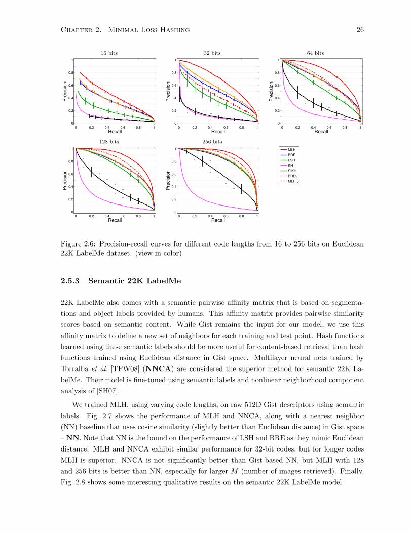
Chapter 2. Minimal Loss Hashing 26
16 bits 32 bits 64 bits
0 0.2 0.4 0.6 0.8 1
0
0.2
0.4
0.6
0.8
1
Recall
Pre
cis
ion
0 0.2 0.4 0.6 0.8 1
0
0.2
0.4
0.6
0.8
1
Recall
Pre
cis
ion
0 0.2 0.4 0.6 0.8 1
0
0.2
0.4
0.6
0.8
1
Recall
Pre
cis
ion
128 bits 256 bits
0 0.2 0.4 0.6 0.8 1
0
0.2
0.4
0.6
0.8
1
Recall
Pre
cis
ion
0 0.2 0.4 0.6 0.8 1
0
0.2
0.4
0.6
0.8
1
Recall
Pre
cis
ion
0 0.5 1 0
0.2
0.4
0.6
0.8 1
MLH
BRE
LSH
SH
SIKH
BRE2
MLH.5
Figure 2.6: Precision-recall curves for different code lengths from 16 to 256 bits on Euclidean22K LabelMe dataset. (view in color)
2.5.3 Semantic 22K LabelMe
22K LabelMe also comes with a semantic pairwise affinity matrix that is based on segmenta-
tions and object labels provided by humans. This affinity matrix provides pairwise similarity
scores based on semantic content. While Gist remains the input for our model, we use this
affinity matrix to define a new set of neighbors for each training and test point. Hash functions
learned using these semantic labels should be more useful for content-based retrieval than hash
functions trained using Euclidean distance in Gist space. Multilayer neural nets trained by
Torralba et al. [TFW08] (NNCA) are considered the superior method for semantic 22K La-
belMe. Their model is fine-tuned using semantic labels and nonlinear neighborhood component
analysis of [SH07].
We trained MLH, using varying code lengths, on raw 512D Gist descriptors using semantic
labels. Fig. 2.7 shows the performance of MLH and NNCA, along with a nearest neighbor
(NN) baseline that uses cosine similarity (slightly better than Euclidean distance) in Gist space
– NN. Note that NN is the bound on the performance of LSH and BRE as they mimic Euclidean
distance. MLH and NNCA exhibit similar performance for 32-bit codes, but for longer codes
MLH is superior. NNCA is not significantly better than Gist-based NN, but MLH with 128
and 256 bits is better than NN, especially for larger M (number of images retrieved). Finally,
Fig. 2.8 shows some interesting qualitative results on the semantic 22K LabelMe model.
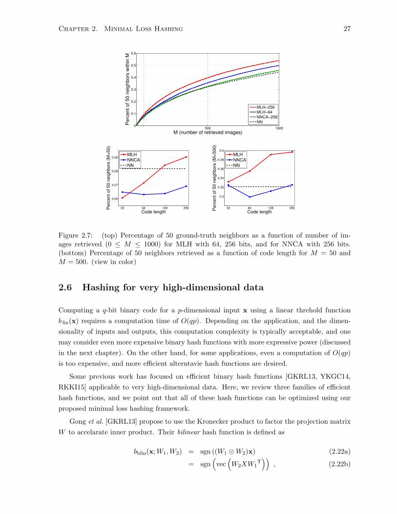
Chapter 2. Minimal Loss Hashing 27
500 10000
0.1
0.2
0.3
0.4
0.5
0.6
M (number of retrieved images)P
erc
ent of 50 n
eig
hbors
within
M
MLH−256
MLH−64NNCA−256
NN
32 64 128 256
0.06
0.07
0.08
0.09
Code length
Perc
ent of 50 n
eig
hbors
(M
=50)
MLHNNCANN
32 64 128 256
0.3
0.32
0.34
0.36
0.38
0.4
Code lengthP
erc
ent of 50 n
eig
hbors
(M
=500)
MLHNNCANN
Figure 2.7: (top) Percentage of 50 ground-truth neighbors as a function of number of im-ages retrieved (0 ≤ M ≤ 1000) for MLH with 64, 256 bits, and for NNCA with 256 bits.(bottom) Percentage of 50 neighbors retrieved as a function of code length for M = 50 andM = 500. (view in color)
2.6 Hashing for very high-dimensional data
Computing a q-bit binary code for a p-dimensional input x using a linear threhold function
b lin(x) requires a computation time of O(qp). Depending on the application, and the dimen-
sionality of inputs and outputs, this computation complexity is typically acceptable, and one
may consider even more expensive binary hash functions with more expressive power (discussed
in the next chapter). On the other hand, for some applications, even a computation of O(qp)
is too expensive, and more efficient alterntavie hash functions are desired.
Some previous work has focused on efficient binary hash functions [GKRL13, YKGC14,
RKKI15] applicable to very high-dimensional data. Here, we review three families of efficient
hash functions, and we point out that all of these hash functions can be optimized using our
proposed minimal loss hashing framework.
Gong et al. [GKRL13] propose to use the Kronecker product to factor the projection matrix
W to accelarate inner product. Their bilinear hash function is defined as
bblin(x;W1,W2) = sgn ((W1 ⊗W2)x) (2.22a)
= sgn(
vec(W2XW1
T))
, (2.22b)

Chapter 2. Minimal Loss Hashing 28
Figure 2.8: Qualitative results on semantic 22K LabelMe. The first image of each row is aquery image. The remaining 13 images on each row were retrieved using 256-bit MLH binarycodes, in increasing order of their Hamming distance.
where ⊗ denotes the Kronecker product, W1,W2 ∈ R√q×√p, and X ∈ R
√p×√p is a matrix whose
entries are identical to that of x, i.e., x = vec (X). Computing a bilinear hash function takes
O(q√p +√qp) which is much better than O(qp). While bilinear hash functions are optimized
using quantization error and two-sided orthogonal procrustes problem in [GKRL13], one can
use our upper bound approach to optimze bblin(x;W1,W2) as well.
Yu et al. [YKGC14] propose a technique called circulant binary embedding, which constrains
the projection matrix W to be a circulant matrix multiplied by a diagonal matrix. A circulant
matrix is a special square matrix in which each row vector is rotated one element to the right
relative to the preceding row vector, so a p by p circulant matrix has only p free parameters.
A circulant binary hash function is defined as
bcir(x;C,D) = sgn (CDx) , (2.23)
where C is a p by p circulant matrix and D is a p by p diagonal matrix. The main benefit of
this approach is that a circulat matrix product can be calculated by Fast Fourier Transform
(FFT) which in O(p log p). Assuming that q ≤ p, which is often the case, the first q bit of
bcir(x) can be taken as the binary code. Minimal loss hashing is applicable to optimization of
circulant matrices too.
Finally, Rastegari et al. [RKKI15] propose to use a sparse W matrix to facilitate fast inner
Chapter 2. Minimal Loss Hashing 29
product. They use an `1 regularizer on W based on a different objective function. We believe
that the loss-based framework that we proposed for learning hash functions in this chapter can
be easily amended with an `1 regularizer to obtain sparse projection matrices.
2.7 Summary
In this chapter, based on the latent structural SVM framework, we formulated minimal loss
hashing (MLH), an approach to learning similarity preserving binary codes under a general
class of pairwise loss functions. We introduced a new loss function, pairwise hinge loss, suitable
for training using Euclidean distance or using sets of similar / dissimilar points. Our learning
algorithm is online, efficient, and scales well to large datasets and large code lengths. We pro-
posed an efficient loss-augmented inference algorithm for optimization of pairwise loss functions.
Empirical results on different datasets suggest that MLH outperforms existing methods.

Chapter 2. Minimal Loss Hashing 30
2.A Proof of the inequlity on the tightness of bound
We present a step by step proof for the following inequality on the tightness of the upper bound
on pairwise hashing loss for any scalar γ > 1,
maxg,g′∈Hq
{`pair(g,g
′, s) + γgTWx + γg′TWx′
}− max
h∈HqγhTWx− max
h′∈Hqγh′
TWx′
≤ maxg,g′∈Hq
{`pair(g,g
′, s) + gTWx + g′TWx′
}− max
h∈HqhTWx− max
h′∈Hqh′
TWx′ .
(2.24)
To prove the inequality (2.24) let
(g, g′) = argmax(g,g′)∈Hq×Hq
{`pair(g,g
′, s) + gTWx + g′TWx′
}, (2.25)
(gγ , g′γ) = argmax(g,g′)∈Hq×Hq
{`pair(g,g
′, s) + γgTWx + γg′TWx′
}. (2.26)
Then, because of (2.25), we know that
`pair(gγ , g′γ , s) + gγTWx + g′γ
TWx′ ≤ `pair(g, g′, s) + gTWx + g′
TWx′ (2.27)
Next, we subract the same quantity from both sides of (2.27) to obtain,
`pair(gγ , g′γ , s) + gγTWx + g′γ
TWx′ − max
h∈HqhTWx− max
h′∈Hqh′
TWx′
≤ `pair(g, g′, s) + gTWx + g′TWx′ − max
h∈HqhTWx− max
h′∈Hqh′
TWx′ .
(2.28)
Note that the RHS of (2.28) is identical to the RHS of (2.24). Below we show the LHS of (2.28)
is larger than the LHS of (2.24), hence the inequality. By definition we know that
gγTWx ≤ max
h∈HqhTWx , (2.29)
g′γTWx′ ≤ max
h′∈Hqh′
TWx′ . (2.30)
Muliplying all of the terms by (γ − 1) and summing over the two sides we get,
(γ − 1)gγTWx + (γ − 1)g′γ
TWx′ ≤ (γ − 1) max
h∈HqhTWx + (γ − 1) max
h′∈Hqh′
TWx′ (2.31)
Adding `pair(gγ , g′γ , s) to both sides and reorganizing the terms we get,
`pair(gγ , g′γ , s) + γgγTWx + γg′γ
TWx′ − γ max
h∈HqhTWx− γ max
h′∈Hqh′
TWx′
≤ `pair(gγ , g′γ , s) + gγTWx + g′γ
TWx′ − max
h∈HqhTWx− max
h′∈Hqh′
TWx′
(2.32)
Now by combining (2.32) and (2.28), we have a proof for inequality (2.24).
Chapter 3
Hamming Distance Metric Learning
Many machine learning algorithms presuppose the existence of a pairwise similarity measure on
the input space. Examples include semi-supervised clustering, nearest neighbor classification,
and kernel-based methods. When similarity measures are not given a priori, one could adopt
a generic function such as Euclidean distance, but this often produces unsatisfactory results.
The goal of distance metric learning techniques is to improve matters by incorporating side
information, and optimizing parametric distance functions such as the Mahalanobis distance
[DKJ+07, GRHS04, SSSN04, WBS06, XNJR02].
Motivated by large-scale multimedia applications, this chapter continues to advocate the
use of discrete mappings, from input features to binary codes. Compact binary codes are re-
markably storage efficient, allowing one to store massive datasets in memory. The Hamming
distance, a natural similarity measure on binary codes, can be computed with just a few machine
instructions per comparison. Further, it has been shown that one can perform exact nearest
neighbor search in Hamming space significantly faster than linear search, with sublinear run-
times [GPY94, NPF12] (e.g., see Chapter 4). By contrast, retrieval based on Mahalanobis dis-
tance requires approximate nearest neighbor search (NNS), for which state-of-the-art methods
(e.g., see [JDS11, ML09]) do not always perform well, especially with massive, high-dimensional
datasets when storage overheads and distance computations become prohibitive.
In this chapter, we introduce a framework for learning a broad class of binary hash functions
based on a triplet ranking loss designed to preserve relative similarity (c.f., [SJ04, FSSM07,
CSSB10]). While certainly useful for preserving metric structure, this loss function is very well
suited to the preservation of semantic similarity. Notably, it can be viewed as a form of local
ranking loss. It is more flexible than the pairwise hinge loss of the previous chapter, and is
shown below to produce superior hash functions.
Our formulation generalizes the minimal loss hashing (MLH) algorithm of Chapter 2. To
optimize hash function parameters we formulate a continuous upper-bound on empirical loss,
with a new form of loss-augmented inference designed for efficient optimization with the pro-
posed triplet loss on the Hamming space. We also present ways to optimize more general
families of hash functions based on non-linear projection of the data by multilayer neural nets.
31

Chapter 3. Hamming Distance Metric Learning 32
To our knowledge, this is one of the most general frameworks for learning a broad class of hash
functions. In particular, many previous loss-based techniques (e.g., [KD09]) are not capable of
optimizing mappings that involve non-linear projections.
Our experiments indicate that the framework is capable of preserving semantic structure on
challenging datasets, namely, MNIST [MNI] and CIFAR-10 [Kri09]. We show that k-nearest
neighbor (kNN) search on the resulting binary codes retrieves items that bear remarkable
similarity to a given query item. To show that the binary representation is rich enough to
capture salient semantic structure, as is common in metric learning, we also report classification
performance on the binary codes. Surprisingly, on these datasets, simple kNN classifiers in
Hamming space are competitive with sophisticated discriminative classifiers, including SVMs
and neural networks. An important appeal of our approach is the scalability of kNN search on
binary codes to billions of data points, and of kNN classification to millions of class labels.
3.1 Formulation
We aim to learn a mapping b(x) : Rp → Hq, while preserving some notion of similarity. This
mapping is parameterized by a real-valued weight vector w as
b(x;w) = sign (f(x;w)) , (3.1)
where sign(.) denotes the element-wise sign function, and f(x;w) : Rp → Rq is a real-valued
transformation. Different forms of f give rise to different families of hash functions:
1. A linear transform f(x) = Wx, where W ∈ Rq×p and w ≡ vec(W ), is the simplest and
most well-studied case [Cha02, GL11, NF11, WKC10] discussed in the previous chapter.
Under this mapping, denoted b lin(x), the kth bit is determined by a hyperplane in the
input space whose normal is given by the kth row of W . 1
2. In [WTF08], linear projections are followed by an element-wise cosine transform, i.e., f(x) =
cos(Wx). For such mappings the bits correspond to stripes of 1 and −1 regions, oriented
parallel to the corresponding hyperplanes, in the input space.
3. Kernelized hash functions [KD09, KG09] make use of a kernel function κ(x, z) and a set
of randomly selected m data points {xπj}mj=1 to define the ith dimension of f denoted fi
via a parameter matrix W ∈ Rq×(m+1) by,
fi(x;W ) = Wi0 +
m∑j=1
Wijκ(xπj ,x) . (3.2)
4. More complex hash functions are obtained with multilayer neural networks [SH09, TFW08].
1For presentation clarity, in linear and nonlinear cases, we omit bias terms. They are incorporated by addingone dimension to the input vectors, and to the hidden layers of neural networks, with a fixed value of one.

Chapter 3. Hamming Distance Metric Learning 33
For example, a two-layer network with a p′-dimensional hidden layer and weight matrices
W1 ∈ Rp′×p and W2 ∈ Rq×p′ can be expressed as f(x) = tanh(W2 tanh(W1x)), where
tanh(.) is the element-wise hyperbolic tangent function.
Our framework applies to all of the above families of hash functions. The only restriction is
that f must be differentiable with respect to its parameters, so that one is able to compute the
Jacobian of f(x;w) with respect to w.
3.1.1 Triplet loss function
The choice of loss function is crucial for learning good similarity measures. Most existing
supervised binary hashing techniques [GL11, LWJ+12, NF11] formulate learning objectives in
terms of pairwise similarity, where pairs of inputs are labelled as either similar or dissimilar.
Next, the methods aim to ensure that Hamming distances between binary codes for similar
(dissimilar) items are small (large). For example, in Chapter 2 we proposed a pairwise hinge
loss function in (2.3). This loss incurs zero cost when a pair of similar inputs map to codes
that differ by less than ρ bits. The loss is zero for dissimilar items whose Hamming distance is
more than ρ bits.
One problem with such a loss function is that finding a suitable threshold ρ with cross-
validation is expensive. Furthermore, for many problems one cares about the relative magni-
tudes of pairwise distances more than their precise numerical values. So, constraining pairwise
Hamming distances over all pairs of codes with a single threshold is overly restrictive. More
importantly, not all datasets are amenable to labeling input pairs as similar or dissimilar. One
way to avoid some of these problems is to define loss in terms of relative similarity. Such loss
a function has been used in metric learning [FSSM07, CSSB10], and, as shown below, it is
naturally suited to Hamming distance metric learning.
To define relative similarity, we assume that the training data includes triplets of items
(x,x+,x−), such that the pair (x,x+) is more similar than the pair (x,x−). Our goal is to
learn a hash function b such that b(x) is closer to b(x+) than to b(x−) in Hamming distance.
Accordingly, we propose a ranking loss on the triplet of binary codes (h,h+,h−), obtained from
b applied to (x,x+,x−):
`rank(h,h+,h−) =[‖h−h+‖H − ‖h−h−‖H + 1
]+. (3.3)
This loss is zero when the Hamming distance between the more-similar pair, ‖h−h+‖H , is at
least one bit smaller than the Hamming distance between the less-similar pair, ‖h−h−‖H . This
loss function is more flexible than the pairwise loss function `hinge, as it can be used to preserve
rankings among similar items, for example based on Euclidean distance, or perhaps using a tree
based distance between category labels within a phylogenetic tree.

Chapter 3. Hamming Distance Metric Learning 34
3.2 Optimization through an upper bound
Given a training set of triplets, D ={
(xi,x+i ,x
−i )}ni=1
, our objective is empirical loss,
L(w) =∑
(x,x+,x−)∈D
`rank(b(x;w), b(x+;w), b(x−;w)
). (3.4)
This objective is discontinuous and non-convex. We again construct a continuous upper bound
on the loss inspired by previous work on latent structural SVMs [YJ09]. The key observation
is that,
b(x;w) = sign (f(x;w)) (3.5a)
= argmaxh∈Hq
hTf(x;w) . (3.5b)
The upper bound on loss that we exploit for learning takes the following form,
`rank(b(x;w), b(x+;w), b(x−;w)
)≤
maxg,g+,g−
{`rank
(g, g+, g−
)+ gTf(x;w) + g+T
f(x+;w) + g−Tf(x−;w)
}−max
h
{hTf(x;w)
}−max
h+
{h+T
f(x+;w)}−max
h−
{h−
Tf(x−;w)
},
(3.6)
where g, g+, g−, h, h+, and h− are constrained to be q-dimensional binary vectors. To
prove the inequality in (3.6), note that if the first term on the RHS were maximized2 by
(g,g+,g−) = (b(x), b(x+), b(x−)), then using (3.5b), it is straightforward to show that (3.6)
would become an equality. In all other cases of (g,g+,g−) which maximize the first term, the
RHS can only be as large or larger than when (g,g+,g−) = (b(x), b(x+), b(x−)), hence the
inequality holds.
Summing the upper bound instead of the loss in (3.4) yields an upper bound on the empirical
loss. The resulting bound is continuous and piecewise smooth in w as long as f is continuous
in w. The upper bound of (3.6) is a generalization of a bound introduced in Section 2.2 for
linear f(x) = Wx. In particular, when f is linear in w, the bound on empirical loss becomes
piecewise linear and convex-concave. While the bound in (3.6) is only piecewise smooth, it
allows us to learn hash functions based on non-linear functions f , e.g., neural networks. Note
that the bound in Section 2.2 was defined for pairwise loss functions and pairwise similarity
labels, and the bound here applies to the more flexible class of triplet loss functions.
Regarding the tightness of the bound, one can echo the proposition (2.11) showing that the
upper bound (3.6) becomes tighter and more non-smooth as ‖f(x)‖ grows. Hence, if f(x) is
not constrained, one should consider regularizing the parameters. For neural networks, we use
a typical weight decay regularizer.
2For presentation clarity we will sometimes drop the dependence of f and b on w, and write b(x) and f(x).

Chapter 3. Hamming Distance Metric Learning 35
3.2.1 Loss-augmented inference with triplet hashing loss
Loss-augmented inference to find the three binary codes given by,
(g, g+, g−) = argmax(g,g+,g−)
{`rank
(g, g+, g−
)+ gTf(x) + g+T
f(x+) + g−Tf(x−)
}, (3.7)
is hard because there are 23q possible binary codes over which one has to maximize the RHS.
We can solve this loss-augmented inference problem efficiently for the class of triplet loss
functions that depend only on the value of
dH(g,g+,g−) ≡ ‖g−g+‖H − ‖g−g−‖H .
Importantly, such loss functions do not depend on the specific binary codes, but rather just the
Hamming distance differences. Note that dH(g,g+,g−) can take on only 2q+1 possible values,
since it is an integer between −q and +q. Clearly the triplet ranking loss only depends on d as,
`rank(g,g+,g−
)= ` ′
(dH(g,g+,g−)
), where ` ′(α) = [α+ 1 ]+ . (3.8)
For this family of loss functions, given the values of f(x), f(x+), and f(x−) in (3.7), loss-
augmented inference can be performed in time O(q2). To show this, first consider the case
dH(g,g+,g−) = m, where m is an integer between −q and q. In this case we can replace the
loss-augmented inference problem with
` ′(m) + maxg,g+,g−
{gTf(x) + g+T
f(x+) + g−Tf(x−)
}s.t. dH(g,g+,g−) = m . (3.9)
One can solve (3.9) for each possible value of m. It is straightforward to see that the largest of
those 2q + 1 maxima is the solution to (3.7). Then, what remains for us is to solve (3.9).
To solve (3.9), consider the kth bit for each of the three codes, i.e., a=g[k], b=g+[k], and
c=g−[k]. There are 8 ways to select a, b and c, but no matter what values they take on, they
can only change the value of dH(g,g+,g−) by −1, 0, or +1. Accordingly, let ek ∈ {−1, 0,+1}denote the effect of the kth bits on dH(g,g+,g−). For each value of ek, we can easily compute
the maximal contribution of (a, b, c) to (3.9) by:
cont(k, ek) = maxa,b,c
{af(x)[k] + bf(x+)[k] + cf(x−)[k]
}s. t. ‖a−b‖H − ‖a−c‖H = ek (3.10)
for a, b, c ∈ {−1,+1}.Therefore, to solve (3.9), we aim to select values for ek ∈ {−1, 0,+1}, for all k, such that
dH(g,g+,g−) =∑q
k=1 ek = m and∑q
k=1 cont(k, ek) is maximized. This can be solved for
any m using a dynamic programming algorithm similar to knapsack, which runs in O(q2).
This dynamic programming algorithm relies on solving a subproblem C(r, s), which seeks the
maximum value of∑r
k=1 cont(k, ek) for the first r bits (0 ≤ r ≤ q) such that∑r
k=1 ek = s for

Chapter 3. Hamming Distance Metric Learning 36
any −r ≤ s ≤ r. One can easily update C(r, s) from its previous values by
C(r, s)← max(C(r − 1, s+ 1) + cont(r,−1),
C(r − 1, s) + cont(r, 0),
C(r − 1, s− 1) + cont(r,+1)).
(3.11)
Note that because the value of∑r
k=1 ek is always between −r and r, we set C(r, s) = −∞ for
any s > r and s < −r. The value of C(0, 0) is initialized at 0. Updating all of the values of
C(r, s) for 1 ≤ r ≤ q and −r ≤ s ≤ r requires a running time of O(q2).
Finally, we choose the best m according to (3.9) as
m = argmax−q≤m≤q
{` ′(m) + C(q,m)
}, (3.12)
and we set the triplet of q-bit codes, (g, g+, g−), according to the ek’s that yield the maximum
of C(q, m) and the bits that maximize cont(k, ek)’s.
3.2.2 Perceptron-like learning with triplet loss
Our learning algorithm is a form of stochastic gradient descent, where in the tth iteration we
sample a triplet (x,x+,x−) from the dataset, and then take a step in the direction that decreases
the upper bound on the triplet’s loss in (3.6). To this end, we randomly initialize w(0). Then,
at each iteration t + 1, given w(t), we use the following procedure to update the parameters,
w(t+1):
1. Select a random triplet (x,x+,x−) from dataset D.
2. Compute (h, h+, h−) = (b(x;w(t)), b(x+;w(t)), b(x−;w(t))) using (3.5b).
3. Compute (g, g+, g−), the solution to the loss-augmented inference problem in (3.7) .
4. Update model parameters using
w(t+1)=w(t) + η
[∂f(x)
∂w
(h−g
)+∂f(x+)
∂w
(h+−g+
)+∂f(x−)
∂w
(h−−g−
)− λw(t)
],
where η is the learning rate, and ∂f(x)/∂w ≡ ∂f(x;w)/∂w|w=w(t) ∈ R|w|×q is the trans-
pose of the Jacobian matrix, where |w| is the number of parameters.
This update rule can be seen as gradient descent in the (regularized) upper bound of the
empirical loss. Although the upper bound in (3.6) is not differentiable at isolated points (owing
to the max terms), in our experiments we find that this update rule consistently decreases both
the upper bound and the actual empirical loss L(w).

Chapter 3. Hamming Distance Metric Learning 37
3.3 Asymmetric Hamming distance
When Hamming distance is used to score and retrieve the nearest neighbors to a given query,
there is a high probability of a tie, where multiple items are equidistant from the query in Ham-
ming space. To break ties and improve the similarity measure, previous work suggests the use
of an asymmetric Hamming (AH) distance [DCL08, GP11]. With an AH distance, one stores
dataset entries as binary codes (for storage efficiency) but the queries are not binarized. An
asymmetric distance function is therefore defined on a real-valued query vector, v ∈ Rq, and a
database binary code, h ∈ Hq. Computing AH distance is slightly less efficient than Hamming
distance, and efficient retrieval algorithms, such as [NPF12], are not directly applicable. Nev-
ertheless, the AH distance can also be used to re-rank items retrieved using Hamming distance,
with a negligible increase in run-time. To improve efficiency further when there are many codes
to be re-ranked, AH distance from the query to binary codes can be pre-computed for each 8
or 16 consecutive bits, and stored in a query-specific lookup table.
In this work, we use the following asymmetric Hamming distance function
AH(h,v; s) =1
4‖h− tanh(diag(s)v) ‖22 , (3.13)
where s ∈ Rq is a vector of scaling parameters that control the slope of hyperbolic tangent
applied to different bits; diag(s) is a diagonal matrix with the elements of s on its diagonal. As
the scaling factors in s approach infinity, AH and Hamming distances become identical. Here
we use the AH distance between a database code b(x) and the real-valued projection for a query
z given by f(z). Based on our validation sets, the AH distance of (3.13) is relatively insensitive
to values in s. For the experiments we simply use s to scale the average absolute values of the
elements of {f(xi)}ni=1 for database entries to be 0.25.
3.4 Implementation details
In practice, the basic learning algorithm described in Section 3.2 is implemented with several
modifications. First, instead of using a single training triplet to estimate the gradients, we
use mini-batches comprising 100 triplets and average the gradient. Second, for each triplet
(x,x+,x−), we replace x− with a “hard” example by selecting an item among all negative
examples in the mini-batch that is closest in the current Hamming distance to b(x). By har-
vesting hard negative examples, we ensure that the Hamming constraints for the triplets are
not too easily satisfied. Third, to find good binary codes, we encourage each bit, averaged
over the training data, to be mean-zero before quantization (motivated in [WTF08]). This is
accomplished by adding the following penalty to the objective function:
1
2‖mean
x
(f(x;w)
)‖22 , (3.14)
Chapter 3. Hamming Distance Metric Learning 38
where mean(f(x;w)) denotes the mean of f(x;w) across the training data. In our implementa-
tion, for efficiency, the stochastic gradient of Eq. 3.14 is computed per mini-batch. Empirically,
we observe that including this term in the objective improves the quality of binary codes,
especially with the triplet ranking loss.
We use a heuristic to adapt learning rates, known as bold driver [Bat89]. For each mini-batch
we evaluate the learning objective before the parameters are updated. As long as the objective
is decreasing we slowly increase the learning rate η, but when the objective increases, η is
halved. In particular, after every 25 epochs, if the objective, averaged over the last 25 epochs,
decreased, we increase η by 5%, otherwise we decrease η by 50%. We also used a momentum
term; i.e., the previous gradient update is scaled by 0.9 and then added to the current gradient.
All experiments are run on a GPU for 2, 000 passes through the datasets. The training time
for our current implementation is under 4 hours of GPU time for most of our experiments. The
two exceptions involve CIFAR-10 with 6400D inputs and relatively long code-lengths of 256
and 512 bits, for which the training times are approximated 8 and 16 hours respectively.
3.5 Experiments
Our experiments evaluate Hamming distance metric learning using two families of hash func-
tions, namely, linear transforms and multilayer neural networks. For each, we examine two loss
functions, the pairwise hinge loss, `hinge in (2.3), and the triplet ranking loss, `rank in (3.3).
Experiments are conducted on two well-known image corpora, MNIST [MNI] and CIFAR-
10 [Kri09]. Ground-truth similarity labels are derived from class labels; items from the same
class are deemed similar. Training triplets are created by taking two items from the same class,
and one item from a different class. This definition of similarity ignores intra-class variations
and the existence of sub-categories, e.g., styles of handwritten fours, or types of airplanes.
Nevertheless, we use these coarse similarity labels to evaluate our framework. To that end,
using items from the test set as queries, we report precision@k, i.e., the fraction of k-nearest
neighbors in Hamming distance that are same-class items. We also show kNN retrieval results
for qualitative inspection. Finally, we report Hamming (H) and asymmetric Hamming (AH)
kNN classification rates on the test sets.
Datasets. The MNIST [MNI] digit dataset contains 60, 000 training and 10, 000 test images
(28×28 pixels) of ten handwritten digits (0 to 9). Of the 60, 000 training images, we set aside
5, 000 for validation. CIFAR-10 [Kri09] comprises 50, 000 training and 10, 000 test color images
(32×32 pixels). Each image belongs to one of 10 classes, namely airplane, automobile, bird, cat,
deer, dog, frog, horse, ship, and truck. The large variability in scale, viewpoint, illumination,
and background clutter poses a significant challenge for classification. Instead of using raw
pixel values, we borrow a bag-of-words representation from Coates et al [CLN11]. Its 6400D
feature vector comprises one 1600-bin histogram per image quadrant, the codewords of which
are learned from 6×6 image patches. Such high-dimensional inputs are challenging for learning
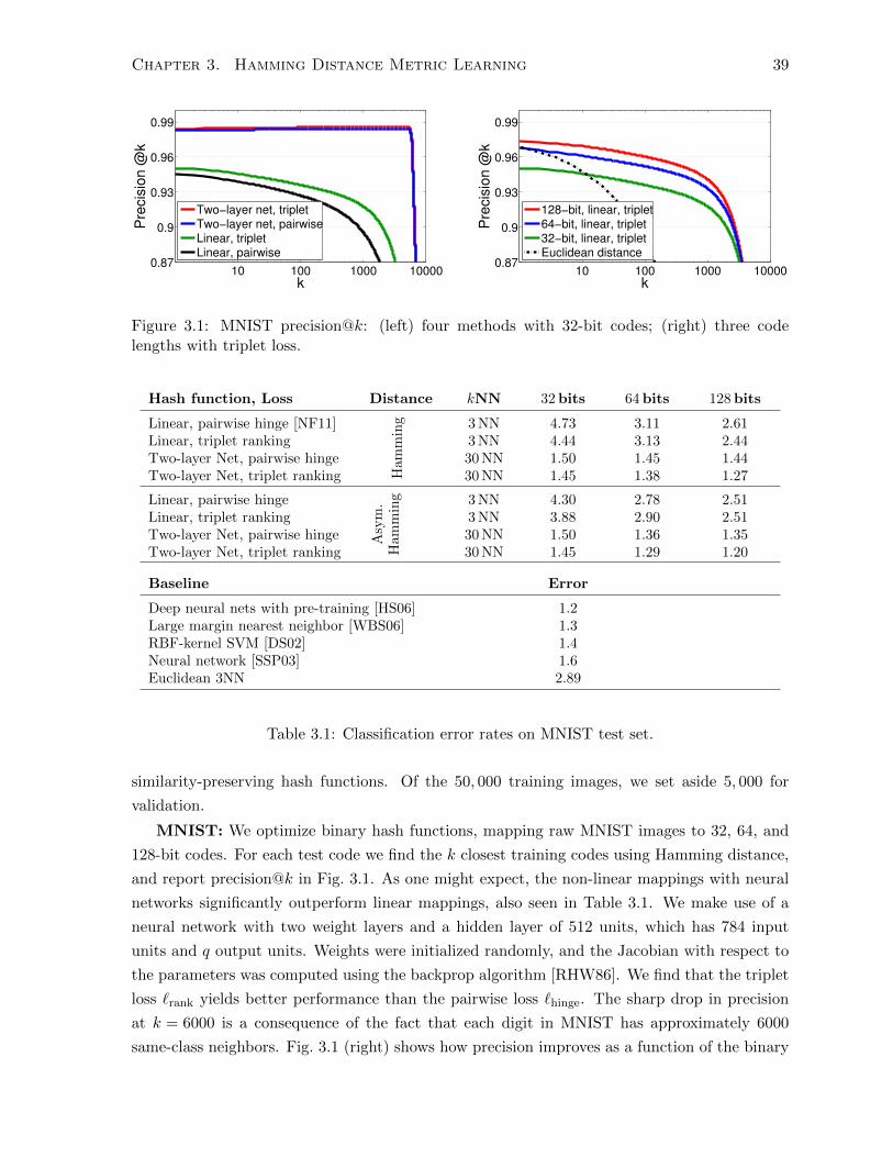
Chapter 3. Hamming Distance Metric Learning 39
10 100 1000 100000.87
0.9
0.93
0.96
0.99
k
Pre
cis
ion @
k
Two−layer net, tripletTwo−layer net, pairwiseLinear, tripletLinear, pairwise
10 100 1000 100000.87
0.9
0.93
0.96
0.99
k
Pre
cis
ion @
k
128−bit, linear, triplet64−bit, linear, triplet32−bit, linear, tripletEuclidean distance
Figure 3.1: MNIST precision@k: (left) four methods with 32-bit codes; (right) three codelengths with triplet loss.
Hash function, Loss Distance kNN 32 bits 64bits 128 bits
Linear, pairwise hinge [NF11]
Ham
min
g 3 NN 4.73 3.11 2.61Linear, triplet ranking 3 NN 4.44 3.13 2.44Two-layer Net, pairwise hinge 30 NN 1.50 1.45 1.44Two-layer Net, triplet ranking 30 NN 1.45 1.38 1.27
Linear, pairwise hinge
Asy
m.
Ham
min
g 3 NN 4.30 2.78 2.51Linear, triplet ranking 3 NN 3.88 2.90 2.51Two-layer Net, pairwise hinge 30 NN 1.50 1.36 1.35Two-layer Net, triplet ranking 30 NN 1.45 1.29 1.20
Baseline Error
Deep neural nets with pre-training [HS06] 1.2Large margin nearest neighbor [WBS06] 1.3RBF-kernel SVM [DS02] 1.4Neural network [SSP03] 1.6Euclidean 3NN 2.89
Table 3.1: Classification error rates on MNIST test set.
similarity-preserving hash functions. Of the 50, 000 training images, we set aside 5, 000 for
validation.
MNIST: We optimize binary hash functions, mapping raw MNIST images to 32, 64, and
128-bit codes. For each test code we find the k closest training codes using Hamming distance,
and report precision@k in Fig. 3.1. As one might expect, the non-linear mappings with neural
networks significantly outperform linear mappings, also seen in Table 3.1. We make use of a
neural network with two weight layers and a hidden layer of 512 units, which has 784 input
units and q output units. Weights were initialized randomly, and the Jacobian with respect to
the parameters was computed using the backprop algorithm [RHW86]. We find that the triplet
loss `rank yields better performance than the pairwise loss `hinge. The sharp drop in precision
at k = 6000 is a consequence of the fact that each digit in MNIST has approximately 6000
same-class neighbors. Fig. 3.1 (right) shows how precision improves as a function of the binary

Chapter 3. Hamming Distance Metric Learning 40
code length. Notably, kNN retrieval, for k > 10 and all code lengths, yields higher precision
than Euclidean NN on the 784D input space. Further, note that these Euclidian kNN results
effectively provide an upper bound on the performance one would expect with existing hashing
methods that preserve Eucliean distances (e.g., [GL11, IM98, KD09, WTF08]).
One can also evaluate the fidelity of the Hamming space represenation in terms of classifi-
cation performance from the Hamming codes. To focus on the quality of the hash functions,
and the speed of retrieval for large-scale multimedia datasets, we use a kNN classifier; i.e., we
just use the retrieved neighbors to predict class labels for each test code. Table 3.1 reports
classification error rates using kNN based on Hamming and asymmetric Hamming distance.
Non-linear mappings, even with only 32-bit codes, significantly outperform linear mappings
(e.g.,with 128 bits). The triplet ranking loss also improves upon the pairwise hinge loss, even
though the former has no hyperparameters. Table 3.1 also indicates that AH distance provides
a modest boost in performance. For each method the parameter k in the kNN classifier is
chosen based on the validation set.
For baseline comparison, Table 3.1 reports state-of-the-art performance on MNIST with
sophisticated discriminative classifiers (excluding those using examplar deformations and con-
volutional nets). Despite the simplicity of a kNN classifier, our model achieves error rates of
1.29% and 1.20% using 64- and 128-bit codes. This is comparable with 1.4% with RBF-SVM
[DS02], and 1.6%, the best published neural net result for this version of the task [SSP03]. Our
model also outperforms the metric learning approach of [WBS06], and is competitive with the
best known Deep Belief Network [HS06]; although they used unsupervised pre-training while
we do not.
The above results show that our Hamming distance metric learning framework can preserve
sufficient semantic similarity, to the extent that Hamming kNN classification becomes com-
petitive with state-of-the-art discriminative methods. Nevertheless, our method is not solely a
classifier, and it can be used within many other machine learning algorithms.
CIFAR-10: On CIFAR-10 we optimize hash functions for 64, 128, 256, and 512-bit codes.
Fig. 3.2 depicts precision@k curves, showing superior quality of hash functions learned by the
ranking loss compared to the pairwise hinge loss. Fig. 3.3 depicts the quality of retrieval results
for four queries from CIFAR-10 test set, showing the 16 nearest neighbors using 256-bit codes,
64-bit codes (both learned with the triplet ranking loss), and Euclidean distance in the original
6400D feature space. The number of class-based retrieval errors is much smaller in Hamming
space, and the similarity in visual appearance is also superior.
Table 3.2 reports classification performance (showing accuracy instead of error rates for
consistency with previous papers). Euclidean kNN on the 6400D input features yields under
60% accuracy, while kNN with the binary codes obtains 76−78%. As with MNIST data, this
level of performance is comparable to one-vs-all SVMs applied to the same features [CLN11].
Not surprisingly, training fully-connected neural nets on 6400-dimensional features with only
50, 000 training examples is challenging and susceptible to over-fitting, hence the results of

Chapter 3. Hamming Distance Metric Learning 41
Triplet ranking loss Pairwise hinge loss
10 100 1000 100000.61
0.64
0.67
0.7
0.73
0.76
0.79
k
Pre
cis
ion @
k
512−bit, linear, triplet256−bit, linear, triplet128−bit, linear, triplet64−bit, linear, triplet
10 100 1000 100000.61
0.64
0.67
0.7
0.73
0.76
0.79
k
Pre
cis
ion @
k
512−bit, linear, pairwise256−bit, linear, pairwise128−bit, linear, pairwise64−bit, linear, pairwise
Figure 3.2: Precision@k plots on the CIFAR-10 dataset for Hamming distance on 512, 256,128, 64-bit codes trained using (left) triplet ranking loss function (right) pairwise hinge loss.Precision is averaged over the test examples.
Hashing, Loss Distance kNN 64 bits 128 bits 256 bits 512 bits
Linear, pairwise hinge (Chapter 2) H 7 NN 72.2 72.8 73.8 74.6Linear, pairwise hinge AH 8 NN 72.3 73.5 74.3 74.9Linear, triplet ranking H 2 NN 75.1 75.9 77.1 77.9Linear, triplet ranking AH 1 NN 75.7 76.8 77.5 78.0
Baseline Accuracy
One-vs-all linear SVM [CLN11] 77.9Euclidean 3NN 59.3
Table 3.2: Recognition accuracy on the CIFAR-10 test set (H ≡ Hamming, AH ≡ Asym.Hamming).
neural nets on CIFAR-10 were not competitive. Previous work [Kri09] had some success training
convolutional neural nets on this dataset. Note that our framework can easily incorporate
convolutional neural nets, which are intuitively better suited to the intrinsic spatial structure
of natural images.
In comparison, another hashing technique called iterative quantization (ITQ) [GL11] achieves
8.5% error on MNIST and 78% accuracy on CIFAR-10. Our method compares favorably, es-
pecially on MNIST. However, note that ITQ [GL11] binarizes the outcome of a supervised
classifier (Canonical Correlation Analysis with labels), and does not explicitly learn a similarity
measure on the input features based on pairs or triplets.
3.6 Summary
We present a framework for Hamming distance metric learning, which entails learning a discrete
mapping from an input space onto binary codes. This framework accommodates different

Chapter 3. Hamming Distance Metric Learning 42
(Hamming on 256 bit codes) (Hamming on 64 bit codes) (Euclidean distance)
Figure 3.3: Retrieval results for four CIFAR-10 test images using Hamming distance on 256-bitand 64-bit codes, and Euclidean distance on bag-of-words features. Red rectangles indicatemistakes.
Chapter 3. Hamming Distance Metric Learning 43
families of hash functions, including linear threshold functions, and quantized multilayer neural
networks. By using a piecewise smooth upper bound on a triplet ranking loss, we optimize hash
functions that are shown to preserve semantic similarity on complex datasets. In particular,
our experiments show that a simple kNN classifier on the learned binary codes is competitive
with sophisticated discriminative classifiers. While other hashing papers have used CIFAR or
MNIST, none report kNN classification performance, often because it has been thought that the
bar established by state-of-the-art classifiers is too high. On the contrary, our kNN classification
performance suggests that Hamming space can be used to represent complex semantic structures
with high fidelity. One appeal of this approach is the scalability of kNN search on binary codes
to billions of data points, and of kNN classification to millions of class labels.

Chapter 4
Fast Exact Search in Hamming
Space with Multi-Index Hashing
There has been growing interest in representing image data and feature descriptors in terms
of compact binary codes, often to facilitate fast near neighbor search and feature matching in
vision applications (e.g., [AOV12, CLSF10, SVD03, SBBF12, TFW08, KGF12]). Binary codes
are storage efficient and comparisons require just a small number of machine instructions.
Millions of binary codes can be compared to a query in less than a second. But the most
compelling reason for binary codes, and discrete codes in general, is their use as direct indices
(addresses) into a hash table, yielding a dramatic increase in search speed compared to an
exhaustive linear scan (e.g., [WTF08, SH09, NF11]).
Nevertheless, using binary codes as direct hash indices is not necessarily efficient. To find
near neighbors one needs to examine all hash table entries (or buckets) within some Hamming
ball around the query. The problem is that the number of such buckets grows near-exponentially
with the search radius. Even with a small search radius, the number of buckets to examine is
often larger than the number of items in the database, and hence slower than linear scan. Recent
papers on binary codes mention the use of hash tables, but resort to linear scan when codes
are longer than 32 bits (e.g., [TFW08, SH09, KD09, NF11]). Not surprisingly, code lengths
are often significantly longer than 32 bits in order to achieve satisfactory retrieval performance
(e.g., see Fig. 4.5).
This chapter presents a new algorithm for exact k-nearest neighbor (kNN) search on binary
codes that is dramatically faster than exhaustive linear scan. This has been an open problem
since the introduction of hashing techniques with binary codes. Our new multi-index hashing
algorithm exhibits sub-linear search times, is storage efficient, and straightforward to implement.
Empirically, on databases of up to 1B codes we find that multi-index hashing is hundreds of
times faster than linear scan. Extrapolation suggests that the speedup gain grows quickly with
database size beyond 1B codes.
44
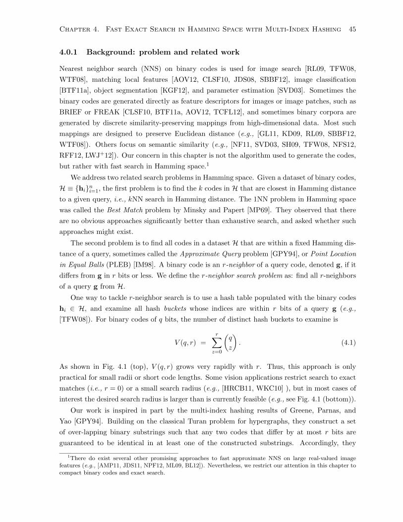
Chapter 4. Fast Exact Search in Hamming Space with Multi-Index Hashing 45
4.0.1 Background: problem and related work
Nearest neighbor search (NNS) on binary codes is used for image search [RL09, TFW08,
WTF08], matching local features [AOV12, CLSF10, JDS08, SBBF12], image classification
[BTF11a], object segmentation [KGF12], and parameter estimation [SVD03]. Sometimes the
binary codes are generated directly as feature descriptors for images or image patches, such as
BRIEF or FREAK [CLSF10, BTF11a, AOV12, TCFL12], and sometimes binary corpora are
generated by discrete similarity-preserving mappings from high-dimensional data. Most such
mappings are designed to preserve Euclidean distance (e.g., [GL11, KD09, RL09, SBBF12,
WTF08]). Others focus on semantic similarity (e.g., [NF11, SVD03, SH09, TFW08, NFS12,
RFF12, LWJ+12]). Our concern in this chapter is not the algorithm used to generate the codes,
but rather with fast search in Hamming space.1
We address two related search problems in Hamming space. Given a dataset of binary codes,
H ≡ {hi}ni=1, the first problem is to find the k codes in H that are closest in Hamming distance
to a given query, i.e., kNN search in Hamming distance. The 1NN problem in Hamming space
was called the Best Match problem by Minsky and Papert [MP69]. They observed that there
are no obvious approaches significantly better than exhaustive search, and asked whether such
approaches might exist.
The second problem is to find all codes in a dataset H that are within a fixed Hamming dis-
tance of a query, sometimes called the Approximate Query problem [GPY94], or Point Location
in Equal Balls (PLEB) [IM98]. A binary code is an r-neighbor of a query code, denoted g, if it
differs from g in r bits or less. We define the r-neighbor search problem as: find all r-neighbors
of a query g from H.
One way to tackle r-neighbor search is to use a hash table populated with the binary codes
hi ∈ H, and examine all hash buckets whose indices are within r bits of a query g (e.g.,
[TFW08]). For binary codes of q bits, the number of distinct hash buckets to examine is
V (q, r) =
r∑z=0
(q
z
). (4.1)
As shown in Fig. 4.1 (top), V (q, r) grows very rapidly with r. Thus, this approach is only
practical for small radii or short code lengths. Some vision applications restrict search to exact
matches (i.e., r = 0) or a small search radius (e.g., [HRCB11, WKC10] ), but in most cases of
interest the desired search radius is larger than is currently feasible (e.g., see Fig. 4.1 (bottom)).
Our work is inspired in part by the multi-index hashing results of Greene, Parnas, and
Yao [GPY94]. Building on the classical Turan problem for hypergraphs, they construct a set
of over-lapping binary substrings such that any two codes that differ by at most r bits are
guaranteed to be identical in at least one of the constructed substrings. Accordingly, they
1There do exist several other promising approaches to fast approximate NNS on large real-valued imagefeatures (e.g., [AMP11, JDS11, NPF12, ML09, BL12]). Nevertheless, we restrict our attention in this chapter tocompact binary codes and exact search.

Chapter 4. Fast Exact Search in Hamming Space with Multi-Index Hashing 46
0 2 4 6 8 100
3
6
9
Hamming Radius
# H
ash
Bu
cke
ts (
log
10)
32 bits
64 bits
128 bits
256 bits
1 10 100 10000
5
10
15
20
# Near neighbors
Ha
mm
ing
Ra
diu
s n
ee
de
d
64 bits
128 bits
Figure 4.1: (Top) Curves show the (log10) number of distinct hash table indices (buckets) withina Hamming ball of radius r, for different code lengths. With 64-bit codes there are about 1Bbuckets within a Hamming ball with a 7-bit radius. Hence with fewer than 1B database items,and a search radius of 7 or more, a hash table would be less efficient than linear scan. Usinghash tables with 128-bit codes is prohibitive for radii larger than 6. (Bottom) This plot showsthe expected search radius required for kNN search as a function of k, based on a dataset of1B SIFT descriptors. Binary codes with 64 and 128 bits were obtained by random projections(LSH) from the SIFT descriptors [JTDA11]. Standard deviation bars help show that largesearch radii are often required.
propose an exact method for finding all r-neighbors of a query using multiple hash tables, one
for each substring. At query time, candidate r-neighbors are found by using query substrings as
indices into their corresponding hash tables. As explained below, while run-time efficient, the
main drawback of their approach is the prohibitive storage required for the requisite number
of hash tables. By comparison, the method we propose requires much less storage, and is only
marginally slower in search performance.
While we focus on exact search, there also exist algorithms for finding approximate r-
neighbors (ε-PLEB), or approximate nearest neighbors (ε-NN) in Hamming distance. One
example is Hamming Locality Sensitive Hashing [IM98, GIM99], which aims to solve the (r, ε)-
neighbors decision problem: determine whether there exists a binary code h ∈ H such that
‖h − g‖H ≤ r, or whether all codes in H differ from g in (1 + ε)r bits or more. Approximate
methods are interesting, and the approach below could be made faster by allowing misses.

Chapter 4. Fast Exact Search in Hamming Space with Multi-Index Hashing 47
Nonetheless, this chapter will focus on the exact search problem.
We proposes a data-structure that applies to both kNN and r-neighbor search in Hamming
space. We prove that for uniformly distributed binary codes of q bits, and a search radius of r
bits when r/q is small, our query time is sub-linear in the size of dataset. We also demonstrate
impressive performance on real-world datasets. To our knowledge this is the first practical
data-structure solving exact kNN in Hamming distance.
Section 4.1 describes a multi-index hashing algorithm for r-neighbor search in Hamming
space, followed by run-time and memory analysis in Section 4.2. Section Section 4.3 describes
our algorithm for k-nearest neighbor search, and Section Section 4.4 reports results on empirical
datasets.
4.1 Multi-Index Hashing
Our approach is a form of multi-index hashing. Binary codes from the database are indexed
m times into m different hash tables, based on m disjoint binary substrings. Given a query
code, entries that fall close to the query in at least one such substring are considered neighbor
candidates. Candidates are then checked for validity using the entire binary code, to remove
any non-r-neighbors. To be practical for large-scale datasets, the substrings must be chosen so
that the set of candidates is small, and storage requirements are reasonable. We also require
that all true neighbors will be found.
The key idea here stems from the fact that, with n binary codes of q bits, the vast majority
of the 2q possible buckets in a full hash table will be empty, since 2q � n. It seems expensive
to examine all V (q, r) buckets within r bits of a query, since most of them contain no items.
Instead, we merge many buckets together (most of which are empty) by marginalizing over
different dimensions of the Hamming space. We do this by creating hash tables on substrings
of the binary codes. The distribution of the code substring comprising the first s bits is the
outcome of marginalizing the distribution of binary codes over the last q − s bits. As such, a
given bucket of the substring hash table includes all codes with the same first s bits, but having
any of the 2(q−s) values for the remaining q − s bits. Unfortunately these larger buckets are
not restricted to the Hamming volume of interest around the query. Hence not all items in the
merged buckets are r-neighbors of the query, so we then need to cull any candidate that is not
a true r-neighbor.
4.1.1 Substring search radii
In more detail, each binary code h, comprising q bits, is partitioned into m disjoint substrings,
h(1), . . . ,h(m), each of length bq/mc or dq/me bits. For convenience in what follows, we assume
that q is divisible2 by m, and that the substrings comprise contiguous bits. The key idea rests
2When q is not divisible by m, we use substrings of different lengths with either b qmc or d q
me bits, i.e., differing
by at most 1 bit.

Chapter 4. Fast Exact Search in Hamming Space with Multi-Index Hashing 48
on the following statement: When two binary codes h and g differ by at most r bits, then, in
at least one of their m substrings they must differ by at most br/mc bits. This leads to the
first proposition:
Proposition 1: If ‖h−g‖H ≤ r, where ‖h−g‖H denotes the Hamming distance between h and
g, then
∃ 1 ≤ z ≤ m s.t. ‖h(z) − g(z)‖H ≤ r′ , (4.2)
where r′ = br/mc.Proof of Proposition 1 follows straightforwardly from the Pigeonhole Principle. That is, suppose
that the Hamming distance between each of the m substrings is strictly greater than r′. Then,
‖h− g‖H ≥ m (r′+ 1). Clearly, m (r′+ 1) > r, since r = mr′+ a for some a where 0 ≤ a < m,
which contradicts the premise.
The significance of Proposition 1 derives from the fact that the substrings have only q/m
bits, and that the required search radius in each substring is just r′ = br/mc. For example, if
h and g differ by 3 bits or less, and m = 4, at least one of the 4 substrings must be identical.
If they differ by at most 7 bits, then in at least one substring they differ by no more than 1
bit; i.e., we can search a Hamming radius of 7 bits by searching a radius of 1 bit on each of
4 substrings. More generally, instead of examining V (q, r) hash buckets, it suffices to examine
V (q/m, r′) buckets in each of m substring hash tables.
While it suffices to examine all buckets within a radius of r′ in all m hash tables, we next
show that it is not always necessary. Rather, it is often possible to use a radius of just r′ − 1
in some of the m substring hash tables while still guaranteeing that all r-neighbors of g will
be found. In particular, with r = mr′ + a, where 0 ≤ a < m, to find any item within a radius
of r on q-bit codes, it suffices to search a + 1 substring hash tables to a radius of r′, and the
remaining m− (a+ 1) substring hash tables up to a radius of r′− 1. Without loss of generality,
since there is no order to the substring hash tables, we search the first a + 1 hash tables with
radius r′, and all remaining hash tables with radius r′ − 1.
Proposition 2: If ||h− g||H ≤ r = mr′ + a, then
∃ 1 ≤ z ≤ a+ 1 s.t. ||h(z) − g(z)||H ≤ r′ (4.3a)
OR
∃ a+ 1 < z ≤ m s.t. ||h(z) − g(z)||H ≤ r′ − 1 . (4.3b)
To prove Proposition 2, we show that when (4.3a) is false, (4.3b) must be true. If (4.3a) is false,
then it must be that a < m−1, since otherwise a = m−1, in which case (4.3a) and Proposition
1 are equivalent. If (4.3a) is false, it also follows that h and g differ in each of their first a+ 1
substrings by r′ + 1 or more bits. Thus, the total number of bits that differ in the first a + 1
substrings is at least (a+1)(r′+1). Because ||h−g||H ≤ r, it also follows that the total number

Chapter 4. Fast Exact Search in Hamming Space with Multi-Index Hashing 49
Algorithm 1 Building m substring hash tables (or direct address tables).
binary code dataset: H = {hi}ni=1
for j = 1 to m doinitialize jth hash table (or direct addres tables)for i = 1 to n do
insert (key = h(j)i , id = i) into jth hash table
end forend for
of bits that differ in the remaining m − (a+1) substrings is at most r − (a+1)(r′+1). Then,
using Proposition 1, the maximum search radius required in each of the remaining m− (a+ 1)
substring hash tables is⌊r − (a+1)(r′+1)
m− (a+1)
⌋=
⌊mr′ + a− (a+1)r′ − (a+1)
m− (a+1)
⌋=
⌊r′ − 1
m− (a+1)
⌋= r′ − 1 , (4.4)
and hence Proposition 2 is true. Because of the near exponential growth in the number of
buckets for large search radii, the smaller substring search radius required by Proposition 2 is
significant.
A special case of Proposition 2 is when r < m, hence r′ = 0 and a = r. In this case, it
suffices to search r+ 1 substring hash tables for a radius of r′ = 0 (i.e., exact matches), and the
remaining m− (r + 1) substring hash tables can be ignored. Clearly, if a code does not match
exactly with a query in any of the selected r+ 1 substrings, then the code must differ from the
query in at least r + 1 bits.
4.1.2 Multi-Index Hashing for r-neighbor search
In a pre-processing step, given a dataset of binary codes, one hash table is built for each of the
m substrings, as outlined in Algorithm 1. Even though we use the term hash table, we make
use of direct address tables when substring length is small and one can allocate 2q/m buckets.
If the substring length is large, one has to use a mapping from binary codes (e.g., taking them
modulo a large prime number) to create smaller number of buckets. At query time, given a
query g with substrings {g(j)}mj=1, we search the jth substring hash table for entries that are
within a Hamming distance of br/mc or br/mc − 1 of g(j), as prescribed by (4.3). By doing
so we obtain a set of candidates from the jth substring hash table, denoted Nj(g). According
to the propositions above, the union of the m sets, N (g) =⋃j Nj(g), is necessarily a superset
of the r-neighbors of g. The last step of the algorithm computes the full Hamming distance
between g and each candidate in N (g), retaining only those codes that are true r-neighbors of
g. Algorithm 2 outlines the r-neighbor retrieval procedure for a query g.

Chapter 4. Fast Exact Search in Hamming Space with Multi-Index Hashing 50
Algorithm 2 r-neighbor search for query g using multi-index hashing with m substrings.
query substrings:{g(j)
}mj=1
initialize mark: for 1 ≤ c ≤ n, set mark[ c ]← falsea← r −mbr/mcfor j = 1 to j ≤ m do
if j ≤ a+ 1 thenρ← br/mc
elseρ← br/mc − 1
end iffor t = 0 to t ≤ ρ do
from jth substring hash table, lookup buckets with keys differing from g(j) in t bitsfor each candidate found with id c doif not mark[ c ] thenmark[ c ]← trueif the code with id c differs from g in at most r bits (full Hamming distance) then
add c to the set of r-neighbor of gend if
end ifend for
end forend for
The query search time depends on the number of buckets examined, lookups, and the number
of candidates tested by full Hamming distance comparison. Some buckets may be empty for
which we only pay the cost of a lookup but not a candidate check. Some canidates may also
be duplicates, for which we only pay the cost of a duplicate detection and not a full Hamming
comparison. Not surprisingly, there is a natural trade-off between the number of lookups and
the number of candidates, controlled by the number of substrings. With a large number of
lookups one can minimize the number of extraneous candidates. By merging many buckets to
reduce the number of lookups, one obtains a large number of candidates to test. In the extreme
case with m = q, substrings are 1 bit long, so we can expect the candidate set to include almost
the entire database.
Note that the idea of building multiple hash tables is not novel in itself (e.g., see [GPY94,
IM98]). However previous work relied heavily on exact matches in substrings. Relaxing this
constraint is what leads to a more effective algorithm, especially in terms of the storage require-
ment.
4.2 Performance analysis
We next develop an analytical model of search performance to help address two key questions:
(1) How does search cost depend on substring length, and hence the number of substrings?
(2) How do run-time and storage complexity depend on database size, code length, and search

Chapter 4. Fast Exact Search in Hamming Space with Multi-Index Hashing 51
radius?
To help answer these questions we exploit a well-known bound on the sum of binomial
coefficients [FG06]; i.e., for any 0 < ε ≤ 12 and η ≥ 1.
bε ηc∑κ=0
(η
κ
)≤ 2H(ε) η , (4.5)
where H(ε) ≡ −ε log2 ε − (1− ε) log2(1− ε) is the entropy of a Bernoulli distribution with
probability ε.
In what follows, n continues to denote the number of q-bit database codes, and r is the
Hamming search radius. Let m denote the number of hash tables, and let s denote the substring
length s = q/m. Hence, the maximum substring search radius becomes r′ = br/mc = bs r/qc.As above, for the sake of model simplicity, we assume q is divisible by m.
We begin by formulating an upper bound on the number of lookups. First, the number of
lookups in Algorithm 2 is bounded above by the product of m, the number of substring hash
tables, and the number of hash buckets within a radius of bs r/qc on substrings of length s bits.
Accordingly, using (4.5), if the search radius is less than half the code length, r ≤ q/2 , then
the total number of lookups is given by
lookups(s) = m
bs r/qc∑z=0
(s
z
)≤ q
s2H(r/q)s . (4.6)
Clearly, as we decrease the substring length s, thereby increasing the number of substrings m,
exponentially fewer lookups are needed.
To analyze the expected number of candidates per bucket, we consider the case in which the
n binary codes are uniformly distributed over the Hamming space. In this case, for a substring
of s bits, for which a substring hash table has 2s buckets, the expected number of items per
bucket is n/2s. The expected size of the candidate set therefore equals the number of lookups
times n/2s.
The total search cost per query is the cost for lookups plus the cost for candidate tests.
While these costs will vary with the code length q and the way the hash tables are implemented,
empirically we find that, to a reasonable approximation, the costs of a lookup and a candidate
test are similar (when q ≤ 256). Accordingly, we model the total search cost per query, for
retrieving all r-neighbors, in units of the time required for a single lookup, as
cost(s) =(
1 +n
2s
) q
s
bsr/qc∑k=0
(s
k
), (4.7)
≤(
1 +n
2s
) q
s2H(r/q)s . (4.8)
In practice, database codes will generally not be uniformly distributed, nor are uniformly
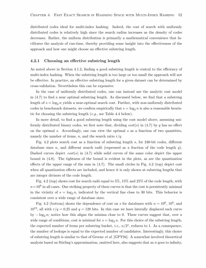
Chapter 4. Fast Exact Search in Hamming Space with Multi-Index Hashing 52
distributed codes ideal for multi-index hashing. Indeed, the cost of search with uniformly
distributed codes is relatively high since the search radius increases as the density of codes
decreases. Rather, the uniform distribution is primarily a mathematical convenience that fa-
cilitates the analysis of run-time, thereby providing some insight into the effectiveness of the
approach and how one might choose an effective substring length.
4.2.1 Choosing an effective substring length
As noted above in Section 4.1.2, finding a good substring length is central to the efficiency of
multi-index hashing. When the substring length is too large or too small the approach will not
be effective. In practice, an effective substring length for a given dataset can be determined by
cross-validation. Nevertheless this can be expensive.
In the case of uniformly distributed codes, one can instead use the analytic cost model
in (4.7) to find a near optimal substring length. As discussed below, we find that a substring
length of s = log2 n yields a near-optimal search cost. Further, with non-uniformly distributed
codes in benchmark datasets, we confirm empirically that s = log2 n is also a reasonable heuris-
tic for choosing the substring length (e.g., see Table 4.4 below).
In more detail, to find a good substring length using the cost model above, assuming uni-
formly distributed binary codes, we first note that, dividing cost(s) in (4.7) by q has no effect
on the optimal s. Accordingly, one can view the optimal s as a function of two quantities,
namely the number of items, n, and the search ratio r/q.
Fig. 4.2 plots search cost as a function of substring length s, for 240-bit codes, different
database sizes n, and different search radii (expressed as a fraction of the code length q).
Dashed curves depict cost(s) in (4.7) while solid curves of the same color depict the upper
bound in (4.8). The tightness of the bound is evident in the plots, as are the quantization
effects of the upper range of the sum in (4.7). The small circles in Fig. 4.2 (top) depict cost
when all quantization effects are included, and hence it is only shown at substring lengths that
are integer divisors of the code length.
Fig. 4.2 (top) shows cost for search radii equal to 5%, 15% and 25% of the code length, with
n=109 in all cases. One striking property of these curves is that the cost is persistently minimal
in the vicinity of s = log2 n, indicated by the vertical line close to 30 bits. This behavior is
consistent over a wide range of database sizes.
Fig. 4.2 (bottom) shows the dependence of cost on s for databases with n = 106, 109, and
1012, all with r/q = 0.25 and q = 128 bits. In this case we have laterally displaced each curve
by − log2 n; notice how this aligns the minima close to 0. These curves suggest that, over a
wide range of conditions, cost is minimal for s = log2 n. For this choice of the substring length,
the expected number of items per substring bucket, i.e., n/2s, reduces to 1. As a consequence,
the number of lookups is equal to the expected number of candidates. Interestingly, this choice
of substring length is similar to that of Greene et al. [GPY94]. A somewhat involved theoretical
analysis based on Stirling’s approximation, omitted here, also suggests that as n goes to infinity,

Chapter 4. Fast Exact Search in Hamming Space with Multi-Index Hashing 53
10 20 30 40 50 60
5
10
15
Substring Length (bits)
Cost (log
10)
r/q = 0.25
r/q = 0.15
r/q = 0.05
−20 −10 0 10 20
5
10
15
Substring Length − log n (bits)
Cost (log
10)
n = 1012
n = 109
n = 106
Figure 4.2: Cost (4.7) and its upper bound (4.8) are shown as functions of substring length(using dashed and solid curves respectively). The code length in all cases is q = 240 bits. (Top)Cost for different search radii, all for a database with n = 109 codes. Circles depict a moreaccurate cost measure, only for substring lengths that are integer divisors of q, and with themore efficient indexing in Algorithm 3. (Bottom) Three database sizes, all with a search radiusof r = 0.25 q. The minima are aligned when each curve is displaced horizontally by − log2 n.
the optimal substring length converges asymptotically to log2 n.
4.2.2 Run-time complexity
Choosing s in the vicinity of log2 n also permits a simple characterization of retrieval run-time
complexity, for uniformly distributed binary codes. When s = log2 n, the upper bound on the
number of lookups (4.6) also becomes a bound on the number candidates. In particular, if we
substitute log2 n for s in (4.8), then we find the following upper bound on the cost, now as a
function of database size, code length, and the search radius:
cost(s) ≤ 2q
log2 nnH(r/q) . (4.9)
Thus, for a uniform distribution over binary codes, if we choose m such that s ≈ log2 n,
the expected query time complexity is O(q nH(r/q)/log2 n). For a small ratio of r/q this is sub-
linear in n. For example, if r/q ≤ .11, then H(.11) < .5, and the run-time complexity becomes

Chapter 4. Fast Exact Search in Hamming Space with Multi-Index Hashing 54
O(b√n/log2 n). That is, the search time increases with the square root of the database size
when the search radius is approximately 10% of the code length. For r/q ≤ .06, this becomes
O(b 3√n/log2 n). The time complexity with respect to q is not as important as that with respect
to n since q is not expected to vary significantly in most applications.
4.2.3 Storage complexity
The storage complexity of our multi-index hashing algorithm is asymptotically optimal when
bq/ log2 nc ≤ m ≤ dq/ log2 ne. To store the full database of binary codes requires O(nq)
bits. For each of m hash tables, we also need to store n unique identifiers to the database
items. This allows one to identify the retrieved items and fetch their full codes; this requires
an additional O(mn log2 n) bits. In sum, the storage required is O(nq + mn log2 n). When
bq/ log2 nc ≤ m ≤ dq/ log2 ne, as is suggested above, this storage cost reduces toO(nq+n log2 n).
Here, the n log2 n term does not cancel as m ≥ 1, but in most interesting cases q > log2 n.
While the storage cost for our multi-index hashing algorithm is linear in nq, the related
multi-index hashing algorithm of Greene et al. [GPY94] entails storage complexity that is super-
linear in n. To find all r-neighbors, for a given search radius r, they construct m = O(r2sr/q)
substrings of length s bits per binary code. Their suggested substring length is also s = log2 n, so
the number of substring hash tables becomes m = O(rnr/q), each of which requires O(n log2 n)
in storage. As a consequence for large values of n, even with small r, this technique requires a
prohibitive amount of memory to store the hash tables.
Our approach is more memory-efficient than that of [GPY94] because we do not enforce
exact equality in substring matching. In essence, instead of creating all of the hash tables
off-line, and then having to store them, we flip bits of each substring at run-time and implicitly
create some of the substring hash tables on-line. This increases run-time slightly, but greatly
reduces storage costs.
4.3 k-Nearest neighbor search
To use the above multi-index hashing in practice, one must specify a Hamming search radius
r. For many tasks, the value of r is chosen such that queries will, on average, retrieve k near
neighbors. Nevertheless, as expected, we find that for many hashing techniques and different
sources of visual data, the distribution of binary codes is such that a single search radius for
all queries will not produce similar numbers of neighbors.
Fig. 4.3 depicts empirical distributions of search radii needed for 10-NN and 1000-NN on
three sets of binary codes obtained from 1B SIFT descriptors [JTDA11, Low04]. In all cases, for
64 and 128-bit codes, and for hash functions based on angular LSH [Cha02] and MLH (Chap-
ter 2), there is a substantial variance in the search radius. This suggests that binary codes are
not uniformly distributed over the Hamming space. As an example, for 1000-NN in 64-bit LSH
codes, more than 10% of the queries require a search radius of 10 bits or larger, while for about

Chapter 4. Fast Exact Search in Hamming Space with Multi-Index Hashing 55
64-bit LSH 64-bit LSH
0 2 4 6 8 10 12 14 160
0.05
0.1
0.15
0.2
0.25
Hamming radii needed for 10−NN
Fra
ction o
f queries
0 2 4 6 8 10 12 14 160
0.05
0.1
0.15
0.2
Hamming radii needed for 1000−NN
Fra
ction o
f queries
128-bit LSH 128-bit LSH
0 5 10 15 20 25 300
0.02
0.04
0.06
0.08
0.1
Hamming radii needed for 10−NN
Fra
ction o
f queries
0 5 10 15 20 25 300
0.02
0.04
0.06
0.08
0.1
Hamming radii needed for 1000−NN
Fra
ction o
f queries
128-bit MLH 128-bit MLH
0 5 10 15 20 25 300
0.02
0.04
0.06
0.08
0.1
0.12
Hamming radii needed for 10−NN
Fra
ction o
f queries
0 5 10 15 20 25 300
0.02
0.04
0.06
0.08
0.1
0.12
Hamming radii needed for 1000−NN
Fra
ction o
f queries
Figure 4.3: Shown are histograms of the search radii that are required to find 10-NN and1000-NN, for 64 and 128-bit code from angular LSH [Cha02], and 128-bit codes from MLH[NF11], based on 1B SIFT descriptors [JTDA11]. Clearly shown are the relatively large searchradii required for both the 10-NN and the 1000-NN tasks, as well as the increase in the radiirequired when using 128 bits versus 64 bits.
10% of the queries it can be 5 bits or smaller. Also evident from Fig. 4.3 is the growth in the
required search radius as one moves from 64-bit codes to 128 bits, and from 10-NN to 1000-NN.
A fixed radius for all queries would produce too many neighbors for some queries, and
too few for others. It is therefore more natural for many tasks to fix the number of required
neighbors, i.e., k, and let the search radius depend on the query. Fortunately, our multi-index
hashing algorithm is easily adapted to accommodate query-dependent search radii.
Given a query, one can progressively increase the Hamming search radius per substring,
until a specified number of neighbors is found. For example, if one examines all r′-neighbors of
a query’s substrings, from which more than k candidates are found to be within a Hamming
distance of (r′ + 1)m− 1 bits in full codes, then it is guaranteed that k-nearest neighbors have
been found. Indeed, if all kNNs of a query g differ from g in r bits or less, then Propositions
1 and 2 above provide guarantees that all such neighbors will be found if one searches the
substring hash tables with the prescribed radii.
In our experiments, we follow this progressive increment of the search radius until we can
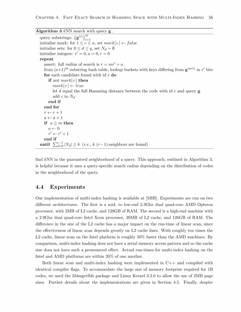
Chapter 4. Fast Exact Search in Hamming Space with Multi-Index Hashing 56
Algorithm 3 kNN search with query g .
query substrings:{g(i)}mi=1
initialize mark: for 1 ≤ c ≤ n, set mark[ c ]← falseinitialize sets: for 0 ≤ d ≤ q, set Nd = ∅initialize integers: r′ = 0, a = 0, r = 0repeat
assert: full radius of search is r = mr′ + a .from (a+1)th substring hash table, lookup buckets with keys differing from g(a+1) in r′ bitsfor each candidate found with id c do
if not mark[ c ] thenmark[ c ]← truelet d equal the full Hamming distance between the code with id c and query gadd c to Nd
end ifend forr ← r + 1a← a+ 1if a ≥ m thena← 0r′ ← r′ + 1
end ifuntil
∑r−1d=0 |Nd| ≥ k (i.e., k (r−1)-neighbors are found)
find kNN in the guaranteed neighborhood of a query. This approach, outlined in Algorithm 3,
is helpful because it uses a query-specific search radius depending on the distribution of codes
in the neighborhood of the query.
4.4 Experiments
Our implementation of multi-index hashing is available at [MIH]. Experiments are run on two
different architectures. The first is a mid- to low-end 2.3Ghz dual quad-core AMD Opteron
processor, with 2MB of L2 cache, and 128GB of RAM. The second is a high-end machine with
a 2.9Ghz dual quad-core Intel Xeon processor, 20MB of L2 cache, and 128GB of RAM. The
difference in the size of the L2 cache has a major impact on the run-time of linear scan, since
the effectiveness of linear scan depends greatly on L2 cache lines. With roughly ten times the
L2 cache, linear scan on the Intel platform is roughly 50% faster than the AMD machines. By
comparison, multi-index hashing does not have a serial memory access pattern and so the cache
size does not have such a pronounced effect. Actual run-times for multi-index hashing on the
Intel and AMD platforms are within 20% of one another.
Both linear scan and multi-index hashing were implemented in C++ and compiled with
identical compiler flags. To accommodate the large size of memory footprint required for 1B
codes, we used the libhugetlbfs package and Linux Kernel 3.2.0 to allow the use of 2MB page
sizes. Further details about the implementations are given in Section 4.5. Finally, despite

Chapter 4. Fast Exact Search in Hamming Space with Multi-Index Hashing 57
0.1 0.2 0.3 0.4 0.5 0.6 0.7 0.8 0.9 10
20
40
60
mem
ory
usage (
GB
)dataset size (billions)
128 bit Linear Scan
128 bit MIH
64 bit Linear Scan
64 bit MIH
Figure 4.4: Memory footprint of our Multi-Index Hashing implementation as a function ofdatabase size. Note that the memory usage does not grow super-linearly with dataset size. Thememory usage is independent of the number of nearest neighbors requested.
DB size = 1M DB size = 1B
250 500 750 10000
0.5
1
k
Eucl
. NN
Rec
all @
k
MLH 128LSH 128MLH 64LSH 64
250 500 750 10000
0.5
1
k
Figure 4.5: Recall rates for BIGANN dataset [JTDA11] (1M and 1B subsets) obtained by kNNon 64- and 128-bit MLH and LSH codes.
the existence of multiple cores, all experiments are run on a single core to simplify run-time
measurements.
The memory requirements for multi-index hashing are described in detail in Section 4.5.
We currently require approximately 27 GB for multi-index hashing with 1B 64-bit codes, and
approximately twice that for 128-bit codes. Fig. 4.4 shows how the memory footprint depends
on the database size for linear scan and multi-index hashing. As explained in the Section 4.2.3,
and demonstrated in Fig. 4.4 the memory cost of multi-index hashing grows linearly in the
database size, as does linear scan. While we use a single computer in our experiments, one
could implement a distributed version of multi-index hashing on computers with much less
memory by placing each substring hash table on a separate computer.

Chapter 4. Fast Exact Search in Hamming Space with Multi-Index Hashing 58
4.4.1 Datasets
We consider two well-known large-scale vision corpora: 80M Gist descriptors from 80 million
tiny images [TFF08] and 1B SIFT features from the BIGANN dataset [JTDA11]. SIFT vec-
tors [Low04] are 128D descriptors of local image structure in the vicinity of feature points. Gist
features [OT01] extracted from 32× 32 images capture global image structure in 384D vectors.
These two feature types cover a spectrum of NNS problems in vision from feature to image
indexing.
We use two similarity-preserving mappings to create datasets of binary codes, namely, binary
angular Locality Sensitive Hashing (LSH) [Cha02], and Minimal Loss Hashing (MLH) (Chap-
ter 2). LSH is considered a baseline random projection method, closely related to cosine simi-
larity. MLH is a state-of-the-art learning algorithm that, given a set of similarity labels, finds
an optimal mapping by minimizing a loss function over pairs or triplets of binary codes.
Both the 80M Gist and 1B SIFT corpora comprise three disjoint sets, namely, a training
set, a base set for populating the database, and a test query set. Using a random permutation,
Gist descriptors are divided into a training set with 300K items, a base set of 79 million items,
and a query set of size 104. The SIFT corpus comes with 100M for training, 109 in the base
set, and 104 test queries.
For LSH we subtract the mean, and pick a set of coefficients from the standard normal
density for a linear projection, followed by quantization. For MLH the training set is used to
optimize hash function parameters. After learning is complete, we remove the training data
and apply the learned hash function to the base set to create the database of binary codes.
With two image corpora (SIFT and Gist), up to three code lengths (64, 128, and 256 bits), and
two hashing methods (LSH and MLH), we obtain several datasets of binary codes with which
to evaluate our multi-index hashing algorithm. Note that 256-bit codes are only used with LSH
and SIFT vectors.
Fig. 4.5 shows Euclidean nearest neighbor recall rates for kNN search on binary codes
generated from 1M and 1B SIFT descriptors. In particular, we plot the fraction of Euclidean
first nearest neighbors found, by kNN in 64-bit and 128-bit LSH and MLH binary codes. As
expected 128-bit codes are more accurate, and MLH outperforms LSH. Note that the multi-
index hashing algorithm solves exact kNN search in Hamming distance; the approximation
that reduces recall is due to the mapping from the original Euclidean space to the Hamming
space. To preserve the Euclidean structure in the original SIFT descriptors, it seems useful
to use longer codes, and exploit data-dependent hash functions such as MLH. Interestingly,
as described below, the speedup factors of multi-index hashing on MLH codes are better than
those for LSH.
Obviously, Hamming distance computed on q-bit binary codes is an integer between 0 and
q. Thus, the nearest neighbors in Hamming distance can be divided into subsets of elements
that have equal Hamming distance (up to q + 1 subsets). Although Hamming distance does
not provide a means to distinguish between equi-distant elements, often a re-ranking phase
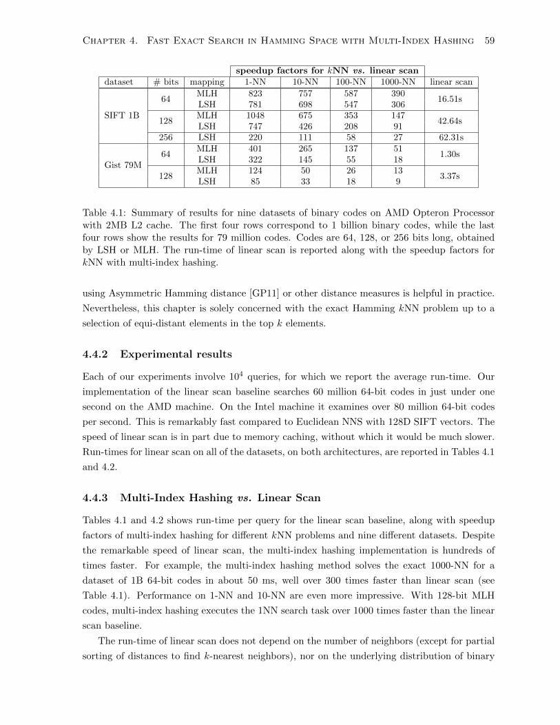
Chapter 4. Fast Exact Search in Hamming Space with Multi-Index Hashing 59
speedup factors for kNN vs. linear scandataset # bits mapping 1-NN 10-NN 100-NN 1000-NN linear scan
SIFT 1B
64MLH 823 757 587 390
16.51sLSH 781 698 547 306
128MLH 1048 675 353 147
42.64sLSH 747 426 208 91
256 LSH 220 111 58 27 62.31s
Gist 79M64
MLH 401 265 137 511.30s
LSH 322 145 55 18
128MLH 124 50 26 13
3.37sLSH 85 33 18 9
Table 4.1: Summary of results for nine datasets of binary codes on AMD Opteron Processorwith 2MB L2 cache. The first four rows correspond to 1 billion binary codes, while the lastfour rows show the results for 79 million codes. Codes are 64, 128, or 256 bits long, obtainedby LSH or MLH. The run-time of linear scan is reported along with the speedup factors forkNN with multi-index hashing.
using Asymmetric Hamming distance [GP11] or other distance measures is helpful in practice.
Nevertheless, this chapter is solely concerned with the exact Hamming kNN problem up to a
selection of equi-distant elements in the top k elements.
4.4.2 Experimental results
Each of our experiments involve 104 queries, for which we report the average run-time. Our
implementation of the linear scan baseline searches 60 million 64-bit codes in just under one
second on the AMD machine. On the Intel machine it examines over 80 million 64-bit codes
per second. This is remarkably fast compared to Euclidean NNS with 128D SIFT vectors. The
speed of linear scan is in part due to memory caching, without which it would be much slower.
Run-times for linear scan on all of the datasets, on both architectures, are reported in Tables 4.1
and 4.2.
4.4.3 Multi-Index Hashing vs. Linear Scan
Tables 4.1 and 4.2 shows run-time per query for the linear scan baseline, along with speedup
factors of multi-index hashing for different kNN problems and nine different datasets. Despite
the remarkable speed of linear scan, the multi-index hashing implementation is hundreds of
times faster. For example, the multi-index hashing method solves the exact 1000-NN for a
dataset of 1B 64-bit codes in about 50 ms, well over 300 times faster than linear scan (see
Table 4.1). Performance on 1-NN and 10-NN are even more impressive. With 128-bit MLH
codes, multi-index hashing executes the 1NN search task over 1000 times faster than the linear
scan baseline.
The run-time of linear scan does not depend on the number of neighbors (except for partial
sorting of distances to find k-nearest neighbors), nor on the underlying distribution of binary
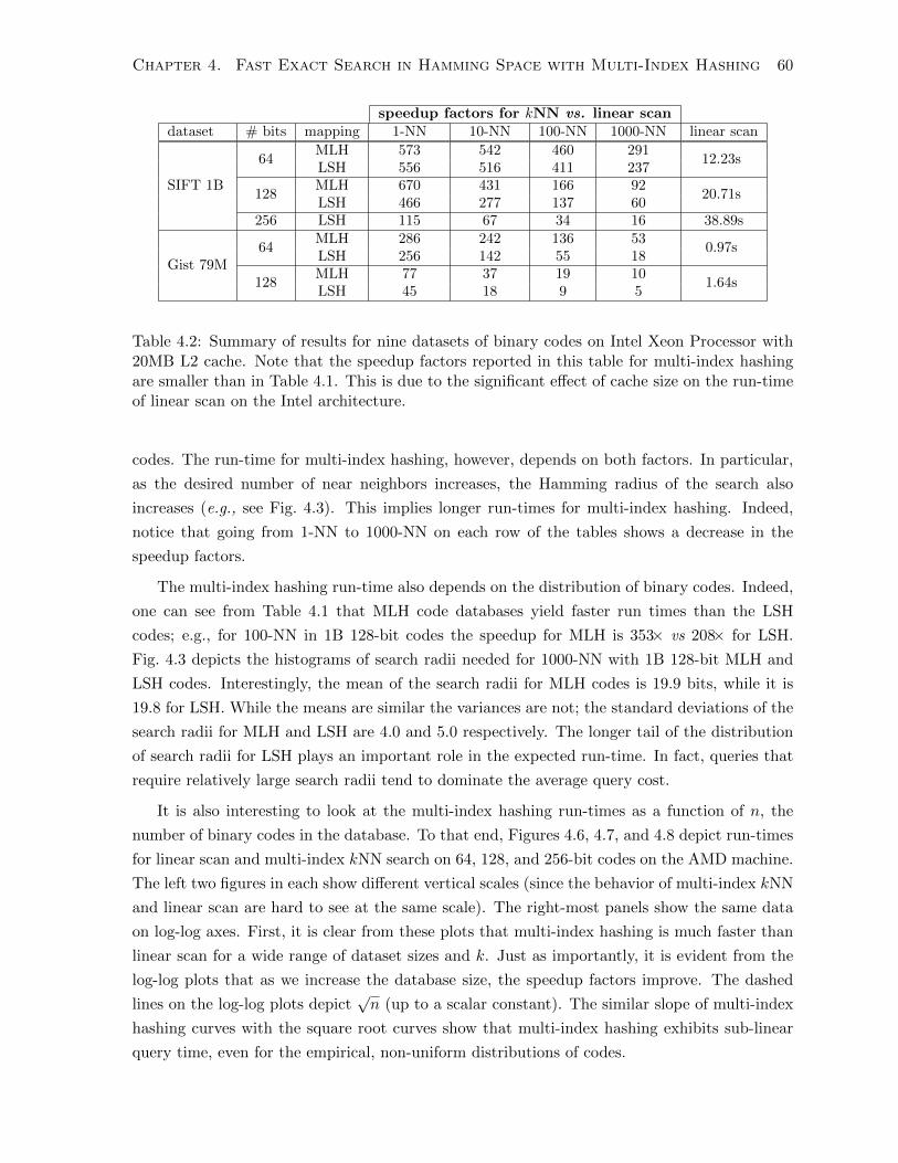
Chapter 4. Fast Exact Search in Hamming Space with Multi-Index Hashing 60
speedup factors for kNN vs. linear scandataset # bits mapping 1-NN 10-NN 100-NN 1000-NN linear scan
SIFT 1B
64MLH 573 542 460 291
12.23sLSH 556 516 411 237
128MLH 670 431 166 92
20.71sLSH 466 277 137 60
256 LSH 115 67 34 16 38.89s
Gist 79M64
MLH 286 242 136 530.97s
LSH 256 142 55 18
128MLH 77 37 19 10
1.64sLSH 45 18 9 5
Table 4.2: Summary of results for nine datasets of binary codes on Intel Xeon Processor with20MB L2 cache. Note that the speedup factors reported in this table for multi-index hashingare smaller than in Table 4.1. This is due to the significant effect of cache size on the run-timeof linear scan on the Intel architecture.
codes. The run-time for multi-index hashing, however, depends on both factors. In particular,
as the desired number of near neighbors increases, the Hamming radius of the search also
increases (e.g., see Fig. 4.3). This implies longer run-times for multi-index hashing. Indeed,
notice that going from 1-NN to 1000-NN on each row of the tables shows a decrease in the
speedup factors.
The multi-index hashing run-time also depends on the distribution of binary codes. Indeed,
one can see from Table 4.1 that MLH code databases yield faster run times than the LSH
codes; e.g., for 100-NN in 1B 128-bit codes the speedup for MLH is 353× vs 208× for LSH.
Fig. 4.3 depicts the histograms of search radii needed for 1000-NN with 1B 128-bit MLH and
LSH codes. Interestingly, the mean of the search radii for MLH codes is 19.9 bits, while it is
19.8 for LSH. While the means are similar the variances are not; the standard deviations of the
search radii for MLH and LSH are 4.0 and 5.0 respectively. The longer tail of the distribution
of search radii for LSH plays an important role in the expected run-time. In fact, queries that
require relatively large search radii tend to dominate the average query cost.
It is also interesting to look at the multi-index hashing run-times as a function of n, the
number of binary codes in the database. To that end, Figures 4.6, 4.7, and 4.8 depict run-times
for linear scan and multi-index kNN search on 64, 128, and 256-bit codes on the AMD machine.
The left two figures in each show different vertical scales (since the behavior of multi-index kNN
and linear scan are hard to see at the same scale). The right-most panels show the same data
on log-log axes. First, it is clear from these plots that multi-index hashing is much faster than
linear scan for a wide range of dataset sizes and k. Just as importantly, it is evident from the
log-log plots that as we increase the database size, the speedup factors improve. The dashed
lines on the log-log plots depict√n (up to a scalar constant). The similar slope of multi-index
hashing curves with the square root curves show that multi-index hashing exhibits sub-linear
query time, even for the empirical, non-uniform distributions of codes.

Chapter 4. Fast Exact Search in Hamming Space with Multi-Index Hashing 61
0.1 0.2 0.3 0.4 0.5 0.6 0.7 0.8 0.9 10
5
10
15
tim
e p
er
query
(s)
dataset size (billions)
Linear scan
1000−NN
100−NN
10−NN
1−NN
0.1 0.2 0.3 0.4 0.5 0.6 0.7 0.8 0.9 10
0.02
0.04
0.06
tim
e p
er
qu
ery
(s)
dataset size (billions)
Linear scan
1000−NN
100−NN
10−NN
1−NN
4 5 6 7 8 9
−4
−3
−2
−1
0
1
log tim
e p
er
query
(lo
g1
0 s
)
dataset size (log10
)
Linear scan
1000−NN
100−NN
10−NN
1−NN
sqrt(n)
Figure 4.6: Run-times per query for multi-index hashing with 1, 10, 100, and 1000 nearestneighbors, and a linear scan baseline on 1B 64-bit binary codes given by LSH from SIFT. Runon an AMD Opteron processor.
0.1 0.2 0.3 0.4 0.5 0.6 0.7 0.8 0.9 10
10
20
30
40
tim
e p
er
query
(s)
dataset size (billions)
Linear scan
1000−NN
100−NN
10−NN
1−NN
0.1 0.2 0.3 0.4 0.5 0.6 0.7 0.8 0.9 10
0.1
0.2
0.3
0.4
0.5
tim
e p
er
qu
ery
(s)
dataset size (billions)
Linear scan
1000−NN
100−NN
10−NN
1−NN
4 5 6 7 8 9
−4
−3
−2
−1
0
1
log tim
e p
er
query
(lo
g1
0 s
)
dataset size (log10
)
Linear scan
1000−NN
100−NN
10−NN
1−NN
sqrt(n)
Figure 4.7: Run-times per query for multi-index hashing with 1, 10, 100, and 1000 nearestneighbors, and a linear scan baseline on 1B 128-bit binary codes given by LSH from SIFT. Runon an AMD Opteron processor.
0.1 0.2 0.3 0.4 0.5 0.6 0.7 0.8 0.9 10
20
40
60
tim
e p
er
query
(s)
dataset size (billions)
Linear scan
1000−NN
100−NN
10−NN
1−NN
0.1 0.2 0.3 0.4 0.5 0.6 0.7 0.8 0.9 10
0.5
1
1.5
2
2.5
tim
e p
er
qu
ery
(s)
dataset size (billions)
Linear scan
1000−NN
100−NN
10−NN
1−NN
4 5 6 7 8 9
−3
−2
−1
0
1
log tim
e p
er
query
(lo
g1
0 s
)
dataset size (log10
)
Linear scan
1000−NN
100−NN
10−NN
1−NN
sqrt(n)
Figure 4.8: Run-times per query for multi-index hashing with 1, 10, 100, and 1000 nearestneighbors, and a linear scan baseline on 1B 256-bit binary codes given by LSH from SIFT. Runon an AMD Opteron processor.

Chapter 4. Fast Exact Search in Hamming Space with Multi-Index Hashing 62
4.4.4 Direct lookups with a single hash table
An alternative to linear scan and multi-index hashing is to hash the entire codes into a single
hash table, and then use direct hashing with each query. As suggested in the introduction and
Fig. 4.1, although this approach avoids the need for any candidate checking, it may require a
prohibitive number of lookups. Nevertheless, for sufficiently small code lengths or search radii,
it may be effective in practice.
Given the complexity associated with efficiently implementing collision detection in large
hash tables, we do not directly experiment with the single hash table approach. Instead, we
consider the empirical number of lookups one would need, as compared to the number of items
in the database. If the number of lookups is vastly greater than the size of the dataset one
can readily conclude that linear scan is likely to be as fast or faster than direct indexing into a
single hash table.
Fortunately, the statistics of neighborhood sizes and required search radii for kNN tasks are
available from the linear scan and multi-index hashing experiments reported above. For a given
query, one can use the kth nearest neighbor’s Hamming distance to compute the number of
lookups from a single hash table that are required to find all of the query’s k nearest neighbors.
Summed over the set of queries, this provides an indication of the expected run-time.
Fig. 4.9 shows the total number of lookups required for 1-NN and 1000-NN tasks by the
single hash table (SHT) approach and the multi-index hashing (MIH) on 64- and 128-bit LSH
codes from SIFT. They are plotted as a function of the size of the dataset, from 104 to 109
items. For comparison, the plots also show the number of database items, and the number of
operations that were needed for linear scan. Note that Fig. 4.9 has logarithmic scales.
It is evident that with a single hash table the number of lookups is almost always several
orders of magnitude larger than the number of items in the dataset. And not surprisingly, this is
also several orders of magnitude more lookups than required for multi-index hashing. Although
the relative speed of a lookup operation compared to a candidate check, as used in linear scan,
depends on the implementation, there are a few important considerations. Linear scan has
an exactly serial memory access pattern and so can make very efficient use of cache, whereas
lookups in a hash table are inherently random. Furthermore, in any plausible implementation of
a single hash table for 64 bit or longer codes, there will be some penalty for collision detection.
As illustrated in Fig. 4.9, the only cases where a single hash table might potentially be more
efficient than linear scan are with very small codes (64 bits or less), with a large dataset (1
billion items or more), and a small search distances (e.g., for 1-NN). In all other cases, linear
scan requires orders of magnitude fewer operations. With any code length longer than 64 bits,
a single hash table approach is completely infeasible to run, requiring upwards of 15 orders of
magnitude more operations than linear scan for 128-bit codes.

Chapter 4. Fast Exact Search in Hamming Space with Multi-Index Hashing 63
64 bits 128 bits
4 5 6 7 8 90
2
4
6
8
10
12
14
16
18
20
Dataset Size (log10
)
Nu
mb
er
of
Op
era
tio
ns (
log
10)
1000NN SHT
1NN SHT
Linearscan
1000NN MIH
1NN MIH
4 5 6 7 8 90
5
10
15
20
25
30
35
40
Dataset Size (log10
)
Nu
mb
er
of
Op
era
tio
ns (
log
10)
1000NN SHT
1NN SHT
Linearscan
1000NN MIH
1NN MIH
Figure 4.9: The number of lookup operations required to solve exact nearest neighbor searchin hamming space for LSH codes from SIFT features, using the simple single hash table (SHT)approach and multi-index hashing (MIH). Also shown is the number of candidate check oper-ations required to search using linear scan. Note that the axes have a logarithmic scale. Withsmall codes (64 bits), many items (1 billion) and small search distance (1-NN), it is conceivablethat a single hash table might be faster than linear scan. In all other cases, a single hash tablerequires many orders of magnitude more operations than linear scan. Note also that MIH willnever require more operations than a single hash table - in the limit of very large dataset sizes,MIH will use only one hash table and becomes equivalent.
4.4.5 Substring Optimization
The substring hash tables used above have been formed by simply dividing the full codes into
disjoint and consecutive sequences bits. For LSH and MLH, this is equivalent to randomly
assigning bits to substrings.
It natural to ask whether further gains in efficiency are possible by optimizing the assignment
of bits to substrings. In particular, by careful substring optimization one may be able to
maximize the discriminability of the different substrings. In other words, while the radius of
substring search, and hence the number of lookups is determined by the desired search radius
on the full codes, and will remain fixed, by optimizing the assignment of bits to substrings one
might be able to reduce the number of candidates needed to validate.
To explore this idea, we considered a simple method in which bits are assigned to substrings
one by one in a greedy fashion, based on the correlation between bits. In particular, of those
bits not yet assigned, we assign a bit to the next substring that minimizes the maximum
correlation between that bit and all other bits already in that substring. Initialization also
occurs in a greedy manner: A random bit is assigned to the first substring, and we assign the
first bit to substring j that is maximally correlated with the first bit of substring j − 1. This
approach significantly decreases the correlation between bits within a single substring, which
should make the distribution of codes within substring buckets more uniform. Hence, lowering
the number of candidates within a given search radius. Arguably an even better approach would
be to maximize the entropy of the entries within each substring hash table, thereby making

Chapter 4. Fast Exact Search in Hamming Space with Multi-Index Hashing 64
optimized speedup vs. linear scan (consecutive, % improvement)# bits 1-NN 10-NN 100-NN 1000-NN
64 788 (781, 1%) 750 (698, 7%) 570 (547, 4%) 317 (306, 4%)128 826 (747, 10%) 472 (426, 11%) 237 (208, 14%) 103 (91, 12%)256 284 (220, 29%) 138 (111, 25%) 68 (58, 18%) 31 (27, 18%)
Table 4.3: Empirical run-time improvements from optimizing substrings vs. consecutive sub-strings, for 1 billion LSH codes from SIFT features (AMD machine). speedup factors vs. linearscan are shown with optimized and consecutive substrings, and the percent improvement. Allexperiments used 10M codes to compute the correlation between bits for substring optimizationand all results are averaged over 10000 queries each.
0 0.1 0.2 0.3 0.4 0.5 0.6 0.7 0.8 0.9 10
0.02
0.04
0.06
tim
e p
er
qu
ery
(s)
dataset size (millions)
Cons. 10−NN
Cons. 100−NN
Cons. 1000−NN
Opt. 10−NN
Opt. 100−NN
Opt. 1000−NN
0 0.1 0.2 0.3 0.4 0.5 0.6 0.7 0.8 0.9 10
0.1
0.2
0.3
0.4
0.5tim
e p
er
qu
ery
(s)
dataset size (millions)
Cons. 10−NN
Cons. 100−NN
Cons. 1000−NN
Opt. 10−NN
Opt. 100−NN
Opt. 1000−NN
0 0.1 0.2 0.3 0.4 0.5 0.6 0.7 0.8 0.9 10
0.5
1
1.5
2
2.5
tim
e p
er
qu
ery
(s)
dataset size (millions)
Cons. 10−NN
Cons. 100−NN
Cons. 1000−NN
Opt. 10−NN
Opt. 100−NN
Opt. 1000−NN
Figure 4.10: Run-times for multi-index-hashing using codes from LSH on SIFT features withconsecutive (solid) and optimized (dashed) substrings. From left to right: 64-bit, 128-bit,256-bit codes, run on the AMD machine.
the distribution of substrings as uniform as possible. This entropic approach is, however, much
more complicated and left to future work.
The results obtained with the correlation-based greedy algorithm show that optimizing
substrings can provide overall run-time reductions on the order of 20% against consecutive sub-
strings for some cases. Table 4.3 displays the improvements achieved by optimizing substrings
for different codes lengths and different values of k. Fig. 4.10 shows the run-time performance
of optimized substrings.
4.5 Implementation details
Our implementation of multi-index hashing is publicly available at [MIH]. Nevertheless, for the
interested reader we describe some of the important details here.
As explained above, the algorithm hinges on hash tables built on disjoint s-bit substrings
of the binary codes. We use direct address tables for the substring hash tables because the
substrings are usually short (s ≤ 32). Direct address tables explicitly allocate memory for 2s
buckets and store all data points associated with each substring in its corresponding bucket.
There is a one-to-one mapping between buckets and substrings, so no time is spent on collision

Chapter 4. Fast Exact Search in Hamming Space with Multi-Index Hashing 65
detection.
One could implement direct address tables with an array of 2s pointers, some of which may
be null (for empty buckets). On a 64-bit machine, pointers are 8 bytes long, so just storing
an empty address table for s = 32 requires 32 GB (as done in [NPF12]). For greater efficiency
here, we use sparse direct address tables by grouping buckets into sets of 32 elements. For each
bucket group, a 32-bit binary vector encodes whether each bucket in the group is empty or
not. Then, a single pointer per group is used to point to a resizable array that stores the data
points associated with that bucket group. Data points within each array are ordered by their
bucket index. To facilitate fast access, for each non-empty bucket we store the index of the
beginning and the end of the corresponding segment of the resizable array. Compared to the
direct address tables in [NPF12], for s = 32, and bucket groups of size 32, an empty address
table requires only 1.5 GB. Also note that accessing elements in any bucket of the sparse address
table is slightly more expensive than a non-sparse address table, but still O(1).
Memory Requirements: We store one 64-bit pointer for each bucket group, and a 32-bit binary
vector to encode whether buckets in a group are empty; this entails 2(s−5) · (8 + 4) bytes for an
empty s-bit hash table (s ≥ 5), or 1.5 GB when s = 32. Bookkeeping for each resizable array
entails 3 32-bit integers. In our experiments, most bucket groups have at least one non-empty
bucket. Taking this into account, the total storage for an s-bit address table becomes 2(s−5) ·24
bytes (3 GB for s = 32).
For each non-empty bucket within a bucket group, we store a 32-bit integer to indicate the
index of the beginning of the segment of the resizable array corresponding to that bucket. The
number of non-empty buckets is at most mmin(n, 2s), where m is the number of hash tables,
and n is the number of codes. Thus we need an extra mmin(n, 2s) ·4 bytes. For each data point
per hash table we store an ID to reference the full binary code; each ID is 4 bytes since n ≤ 232
for our datasets. This entails 4mn bytes. Finally, storing the full binary codes themselves
requires nms/8 bytes, since q = ms.
The total memory cost is m2(s−5)24 +mmin(n, 2s)4 + 4mn+ nms/8 bytes. For s = log2 n,
this cost is O(nq). For 1B 64-bit codes, and m = 2 hash tables (32 bits each), the cost is 28 GB.
For 128-bit and 256-bit codes our implementation requires 57 GB and 113 GB. Note that the
last two terms in the memory cost for storing IDs and codes are irreducible, but the first terms
can be reduced in a more memory efficient implementation.
Duplicate Candidates: When retrieving candidates from the m substring hash tables, some
codes will be found multiple times. To detect duplicates, and discard them, we allocate one
bit-string with n bits. When a candidate is found we check the corresponding bit and discard
the candidate if it is marked as a duplicate. Before each query we initialize the bit-string to
zero. In practice this has negligible run-time. In theory clearing an n-bit vector requires O(n),
but there are more efficient ways to store an n-bit vector without explicit initialization.
Hamming Distance: To compare a query and a candidate (for multi-index search or linear
scan), we compute the Hamming distance on the full q-bit codes, with one xor operation for

Chapter 4. Fast Exact Search in Hamming Space with Multi-Index Hashing 66
n 104 105 106 2× 10⁶ 5× 10⁶ 107 2× 10⁷ 5× 10⁷ 108 2× 10⁸ 5× 10⁸ 109
q = 64m 5 4 4 3 3 3 3 2 2 2 2 2
q/ log2 n 4.82 3.85 3.21 3.06 2.88 2.75 2.64 2.50 2.41 2.32 2.21 2.14
q = 128m 10 8 8 6 6 5 5 5 5 4 4 4
q/ log2 n 9.63 7.71 6.42 6.12 5.75 5.50 5.28 5.00 4.82 4.64 4.43 4.28
q = 256m 19 15 13 12 11 11 10 10 10 9 9 8
q/ log2 n 19.27 15.41 12.84 12.23 11.50 11.01 10.56 10.01 9.63 9.28 8.86 8.56
Table 4.4: Selected number of substrings used for the experiments, as determined by cross-validation, vs. the suggested number of substrings based on the heuristic q / log2 n.
every 64 bits, followed by a pop count to tally the ones. We used the built-in GCC function
__builtin_popcount for this purpose.
Number of Substrings: The number of substring hash tables we use is determined with a
hold-out validation set of database entries. From that set we estimate the running time of the
algorithm for different choices of m near q / log2 n, and select the m that yields the minimum
run-time. As shown in Table 4.4 this empirical value for m is usually the closest integer to
q / log2 n.
Translation Lookaside Buffer and Huge Pages: Modern processors have an on-chip cache that
holds a lookup table of memory addresses, for mapping virtual addresses to physical addresses
for each running process. Typically, memory is split into 4KB pages, and a process that allocates
memory is given pages by the operating system. The Translation Lookaside Buffer (TLB) keeps
track of these pages. For processes that have large memory footprints (tens of GB), the number
of pages quickly overtakes the size of the TLB (typically about 1500 entries). For processes
using random memory access this means that almost every memory access produces a TLB
miss - the requested address is in a page not cached in the TLB, hence the TLB entry must be
fetched from slow RAM before the requested page can be accessed. This slows down memory
access, and causes volatility in run-times for memory-access intensive processes.
To avoid this problem, we use the libhugetlbfs Linux library. This allows the operating
system to allocate Huge Pages (2MB each) rather than 4KB pages. This reduces the number
of pages; hence it reduces the frequency of TLB misses, improves memory access speed, and
reduces run-time volatility. The increase in speed of multi-index hashing results reported here
compared to those in [NPF12] are attributed to the use of libhugetlbfs.
4.6 Conclusion
This chapter describes a new algorithm for exact nearest neighbor search on large-scale datasets
of binary codes. The algorithm is a form of multi-index hashing that has provably sub-linear
run-time behavior for uniformly distributed codes. It is storage efficient and easy to implement.
We show empirical performance on datasets of binary codes obtained from 1 billion SIFT, and
80 million Gist features. With these datasets we find that, for 64-bit and 128-bit codes, our new

Chapter 4. Fast Exact Search in Hamming Space with Multi-Index Hashing 67
multi-index hashing implementation is often more than two orders of magnitude faster than a
linear scan baseline.
While the basic algorithm is developed in this chapter there are several interesting avenues
for future research. For example our preliminary research shows that log2 n is a good choice for
the substring length, and it should be possible to formulate a sound mathematical basis for this
choice. The assignment of bits to substrings was shown to be important above, however the
algorithm used for this assignment is clearly suboptimal. It is also likely that different substring
lengths might be useful for the different hash tables.
Our theoretical analysis proves sub-linear run-time behavior of the multi-index hashing al-
gorithm on uniformly distributed codes, when search radius is small. Our experiments demon-
strate sub-linear run-time behavior of the algorithm on real datasets, while the binary code in
our experiments are clearly not uniformly distributed3. Bridging the gap between theoretical
analysis and empirical findings for the proposed algorithm remains an open problem. In par-
ticular, we are interested in more realistic assumptions on the binary codes, which still allow
for theoretical analysis of the algorithm.
While the current paper concerns exact nearest-neighbor tasks, it would also be interesting
to consider approximate methods based on the same multi-index hashing framework. Indeed,
there are several ways that one could find approximate rather than the exact nearest neighbors
for a given query. For example, one could stop at a given radius of search, even though kNN
items may not have been found. Alternatively, one might search until a fixed number of unique
candidates have been found, even though all substring hash tables have not been inspected to
the necessary radius. Such approximate algorithms have the potential for even greater efficiency,
and would be the most natural methods to compare to existing approximate methods, such as
Hamming distance LSH. That said, such comparisons are more difficult than for exact methods
since one must take into account not only the storage and run-time costs, but also some measure
of the cost of errors (usually in terms of recall and precision).
Finally, recent results have shown that for many datasets in which the binary codes are
the result of some form of vector quantization, an asymmetric Hamming distance is attractive
[GP11, JDS11]. In such methods, rather than converting the query into a binary code, one
directly compares a real-valued query to the database of binary codes. The advantage is that
the quantization noise entailed in converting the query to a binary string is avoided. Thus, one
can use a more accurate distance in the binary code space to approximate the desired distance
in the original feature space. One simple way to approach asymmetric Hamming distance is
to use multi-index hashing with Hamming distance, and then only use an asymmetric distance
when culling candidates. The development of more interesting and effective methods is another
promising avenue for future work.
3In some of our experiments with 1 billion binary codes, tens of thousands of codes fall into the same bucketof 32-bit substring hash tables. This is extremely unlikely with uniformly distributed codes.

Chapter 5
Cartesian k-means
Techniques for vector quantization, like the well-known k-means algorithm, are used widely in
vision and learning. Common applications include codebook learning for object recognition
[SZ03], approximate nearest neighbor search (NNS) for information retrieval [NS06, PCI+07],
and feature compression to handle very large datasets [PLSP10].
In general terms, quantization techniques partition an input vector space into multiple
regions {Si}ki=1, and map points in each region into region-specific representatives {ci}ki=1,
known as centers. As such, a quantizer q(x) applied to a data point x, can be expressed as
q(x) =
k∑i=1
1(x∈Si) ci , (5.1)
where 1(·) is the usual indicator function.
The quality of a quantizer is expressed in terms of expected distortion, a common measure
of which is squared error ‖x − q(x)‖22. In this case, given centers {ci}, the region to which a
point is assigned with minimal distortion is obtained by Euclidean NNS. The k-means algorithm
can be used to learn k centers from data.
To reduce expected distortion, crucial for many applications, one can shrink region volumes
by increasing k, the number of regions. In practice, however, increasing k results in prohibitive
storage and run-time costs. Even if one resorts to approximate k-means with approximate
NNS [PCI+07] or hierarchical k-means [NS06], it is hard to scale to large k (e.g., k = 264) as
storing the centers is untenable.
This chapter concerns methods for scalable quantization with tractable storage and run-
time costs. Inspired by Product Quantization (PQ), a state-of-the-art algorithm for approxi-
mate NNS with high-dimensional data (e.g., [JDS11]), compositionality is one of the key ideas.
By expressing data in terms of recurring, reusable parts, the representational capacity of com-
positional models grows exponentially in the number of parameters. Compression techniques
like JPEG accomplish this by encoding images as disjoint rectangular patches. PQ divides the
feature space into disjoint subspaces that are quantized independently. Other examples include
68

Chapter 5. Cartesian k-means 69
part-based recognition models (e.g., [TMF07]), and tensor-based models for style-content sep-
aration (e.g., [TF00]). Here, with a compositional parametrization of region centers, we find a
family of models that reduce the encoding cost of k centers down from k to between log2 k and√k. A model parameter controls the trade-off between model fidelity and compactness.
We formulate two related algorithms, Orthogonal k-means (ok-means) and Cartesian k-
means (ck-means). They are natural extensions of k-means, and are closely related to other
hashing and quantization methods. The ok-means algorithm is a generalization of the Iterative
Quantization (ITQ) algorithm for finding similarity preserving binary codes [GL11]. The ck-
means model is an extension of ok-means, and can be viewed as a generalization of PQ. A
similar generalization of PQ, called optimized product quantization, was developed concurrently
by Ge, He, Ke and Sun, and also appeared in CVPR 2013 [GHKS13].
We evaluate ok-means and ck-means experimentally on large-scale approximate NNS tasks,
and on codebook learning for recognition. For NNS we use datasets of 1M GIST and 1B
SIFT features, with both symmetric and asymmetric distance measures on the latent codes.
We consider codebook learning for a generic form of recognition on CIFAR-10. In all cases,
ck-means delivers impressive performance.
5.1 k-means
Given a dataset of n p-dimensional points, D ≡ {xj}nj=1, the k-means algorithm partitions the
n points into k clusters, and represents each cluster by a center point. Let C ∈ Rp×k be a
matrix whose columns comprise the k cluster centers, i.e., C = [c1, c2, · · · , ck]. The k-means
objective is to minimize the within-cluster squared distances:
`k-means(C) =∑x∈D
mini‖x− ci‖22
=∑x∈D
minb∈H1/k
‖x− Cb‖22 (5.2)
where H1/k ≡ {b |b ∈ {0, 1}k and ‖b‖2 = 1}, i.e., b is a binary vector comprising a 1-of-
k encoding. Lloyd’s k-means algorithm [Llo82] finds a local minimum of (5.2) by iterative,
alternating optimization with respect to C and the b’s.
The k-means model is simple and intuitive, using NNS to assign points to centers. The
assignment of points to centers can be represented with a log k-bit index per data point. The
cost of storing the centers grows linearly with k.
5.2 Orthogonal k-means with 2m centers
With a compositional model one can represent cluster centers more efficiently. One such
approach is to reconstruct each input with an additive combination of the columns of C.

Chapter 5. Cartesian k-means 70
To this end, instead of the 1-of-k encoding in (5.2), we let b be a general m-bit vector,
b ∈ H′m ≡ {0, 1}m, and C ∈ Rp×m. As such, each cluster center is the sum of a subset of
the columns of C. There are 2m possible subsets, and therefore k = 2m centers. While the
number of parameters in the quantizer is linear in m, the number of centers increases exponen-
tially.
While efficient in representing cluster centers, the approach is problematic, because solving
b = argminb∈H′m
‖x− Cb‖22 , (5.3)
is intractable; i.e., the discrete optimization is not submodular. Obviously, for small 2m one
could generate all possible centers and then perform NNS to find the optimal solution, but this
would not scale well to large values of m.
One key observation is that if the columns of C are orthogonal, then optimization (5.3)
becomes tractable. To explain this, without loss of generality, assume the bits belong to {−1, 1}instead of {0, 1}, i.e., b′ ∈ Hm ≡ {−1, 1}m. Then,
‖x− Cb′‖22 = xTx + b′TCTCb′ − 2xTCb′ . (5.4)
For diagonal CTC, the middle quadratic term on the RHS becomes trace(CTC), independent
of b′. As a consequence, when C has orthogonal columns, one can easily see that,
argminb′∈Hm
‖x− Cb′ ‖22 = sign(CTx) , (5.5)
where sign(·) is the element-wise sign function.
To reduce quantization error further we can also introduce an offset, denoted µ ∈ Rp, to
translate x. Taken together with (5.5), this leads to the loss function for the model we call
orthogonal k-means (ok-means):1
`ok-means(C,µ) =∑x∈D
minb′∈Hm
‖x− µ− Cb′‖22 . (5.6)
Clearly, with a change of variables, b′ = 2b− 1, we can define new versions of µ and C, with
identical loss, for which the unknowns are binary, but in {0, 1}m.
The ok-means quantizer encodes each data point as a vertex of a transformed m-dimensional
unit hypercube. The transform, via C and µ, maps the hypercube vertices onto the input feature
space, ideally as close as possible to the data points. The matrix C has orthogonal columns
and can therefore be expressed in terms of rotation and scaling; i.e., C ≡ RD, where R ∈ Rp×m
has orthonormal columns (RTR = Im), and D ∈ Rm×m is diagonal and positive definite. The
goal of learning is to find the parameters, R, D, and µ, which minimize quantization error.
Fig. 5.1 depicts a small set of 2D data points (red x’s) and two possible quantizations.
1While closely related to ITQ, we use the term ok-means to emphasize the relationship to k-means.
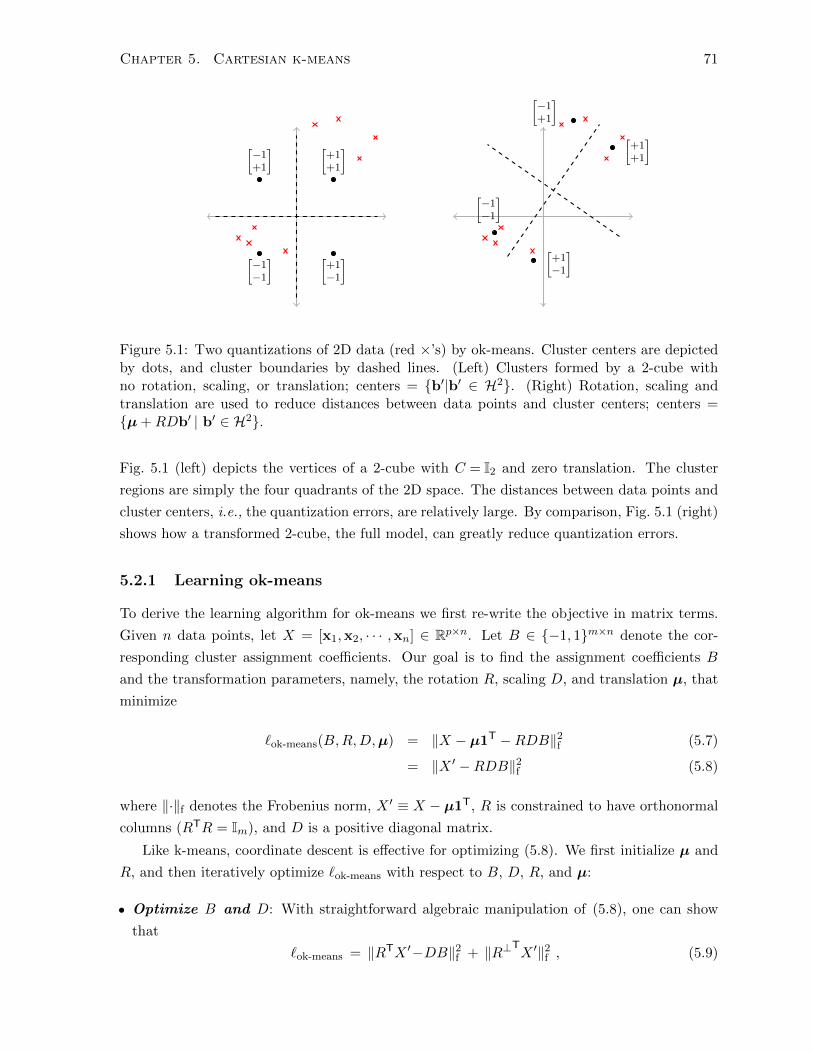
Chapter 5. Cartesian k-means 71
[+1+1
][−1+1
]
[+1−1
][−1−1
]
[−1+1
]
[−1−1
]
[+1+1
]
[+1−1
]
Figure 5.1: Two quantizations of 2D data (red ×’s) by ok-means. Cluster centers are depictedby dots, and cluster boundaries by dashed lines. (Left) Clusters formed by a 2-cube withno rotation, scaling, or translation; centers = {b′|b′ ∈ H2}. (Right) Rotation, scaling andtranslation are used to reduce distances between data points and cluster centers; centers ={µ +RDb′ | b′ ∈ H2}.
Fig. 5.1 (left) depicts the vertices of a 2-cube with C = I2 and zero translation. The cluster
regions are simply the four quadrants of the 2D space. The distances between data points and
cluster centers, i.e., the quantization errors, are relatively large. By comparison, Fig. 5.1 (right)
shows how a transformed 2-cube, the full model, can greatly reduce quantization errors.
5.2.1 Learning ok-means
To derive the learning algorithm for ok-means we first re-write the objective in matrix terms.
Given n data points, let X = [x1,x2, · · · ,xn] ∈ Rp×n. Let B ∈ {−1, 1}m×n denote the cor-
responding cluster assignment coefficients. Our goal is to find the assignment coefficients B
and the transformation parameters, namely, the rotation R, scaling D, and translation µ, that
minimize
`ok-means(B,R,D,µ) = ‖X − µ1T −RDB‖2f (5.7)
= ‖X ′ −RDB‖2f (5.8)
where ‖·‖f denotes the Frobenius norm, X ′ ≡ X − µ1T, R is constrained to have orthonormal
columns (RTR = Im), and D is a positive diagonal matrix.
Like k-means, coordinate descent is effective for optimizing (5.8). We first initialize µ and
R, and then iteratively optimize `ok-means with respect to B, D, R, and µ:
• Optimize B and D: With straightforward algebraic manipulation of (5.8), one can show
that
`ok-means = ‖RTX ′−DB‖2f + ‖R⊥TX ′‖2f , (5.9)

Chapter 5. Cartesian k-means 72
where columns of R⊥ span the orthogonal complement of the column-space of R (i.e., the
block matrix [R R⊥] is orthogonal).
It follows that, given X ′ and R, we can optimize the first term in (5.9) to solve for B and
D. Here, DB is the least-squares approximation to RTX ′, where RTX ′ and DB are m×n.
Further, the ith row of DB can only contain elements from {−di,+di} where di = Dii.
Wherever the corresponding element of RTX ′ is positive (negative) we should put a positive
(negative) value in DB. The optimal di is determined by the mean absolute value of the
elements in the ith row of RTX ′:
B ← sign(RTX ′
)(5.10)
D ← Diag(meanrow
(abs(RTX ′))) (5.11)
• Optimize R: Using the objective (5.8), find the matrix R that minimizes ‖X ′−RA‖2f , subject
to RTR = Im, and A ≡ DB. This is equivalent to an Orthogonal Procrustes problem [Sch66],
and can be solved exactly using SVD. In particular, by adding p − m rows of zeros to the
bottom of D, DB becomes p × n. Then R is square and orthogonal and can be estimated
with SVD. But since DB is degenerate we are only interested in the first m columns of R.
The remaining columns of R are unique only up to rotation of the null-space.
• Optimize µ: Given R, B and D, the optimal µ is given by the column average of X−RDB:
µ ← meanrow
(X−RDB) (5.12)
5.2.2 Distance estimation for approximate nearest neighbor search
One application of scalable quantization is distance estimation for approximate NNS. Before
introducing more advanced quantization techniques, we describe some experimental results
with ok-means on Euclidean approximate NNS. The benefits of ok-means for approximate NNS
are two-fold. Storage costs for the centers is reduced to O(log k), from O(k) with k-means.
Second, substantial speedups are possible by exploiting fast methods for NNS on binary codes
in Hamming space (e.g., Chapter 4).
Generally, in terms of a generic quantizer q(·), there are two natural ways to estimate the
distance between two vectors, z and x [JDS11]. Using the Symmetric quantizer distance (SQD)
‖z−x‖ is approximated by ‖q(z)−q(x)‖. Using the Asymmetric quantizer distance (AQD),
only one of the two vectors is quantized, and ‖z−x‖ is estimated as ‖z−q(x)‖. While SQD
might be slightly faster to compute, AQD incurs lower quantization errors, and hence is more
accurate.
For approximate NNS, in a pre-processing stage, each database entry, x, is encoded into a
binary vector corresponding to the cluster center index to which x is assigned. At test time,
the queries may or may not be encoded into indices, depending on whether one uses SQD or
AQD. The main benefit is that just using quantized dataset entries, one can obtain a good

Chapter 5. Cartesian k-means 73
approximation of distances.
In the ok-means model, the quantization of an input x is straightforwardly shown to be
qok(x) = µ +RD sign(RT(x− µ)) . (5.13)
The corresponding m-bit cluster index is sign(RT(x − µ)). Given two indices, b1,b2 ∈ Hm,
the symmetric ok-means quantizer distance is,
SQDok(b1,b2) = ‖µ +RDb1 − µ−RDb2‖22 (5.14)
= ‖D(b1 − b2)‖22 . (5.15)
In effect, SQDok is a weighted Hamming distance. It is the sum of the squared diagonal entries
of D corresponding to bits where b1 and b2 differ. Interestingly, in our experiments with ok-
means, Hamming and weighted Hamming distances yield similar results. Thus, in ok-means
experiments we simply report results for Hamming distance, to facilitate comparisons with other
hashing techniques. When the scaling in ok-means is constrained to be isotropic (i.e., D = αImfor α ∈ R+), then SQDok becomes a constant multiple of the usual Hamming distance. As
discussed in Section 5.4, this isotropic ok-means is almost identical to ITQ [GL11].
The ok-means defines AQD between a feature vector z and a cluster index b as,
AQDok(z,b) = ‖z− µ−RDb‖22 (5.16)
= ‖RTz′ −Db‖22 + ‖R⊥Tz′‖22 , (5.17)
where z′ = z−µ. For approximate NNS, in comparing distances from query z to a dataset of
binary indices, the second term on the RHS of (5.17) is irrelevant, since it is a constant, which
does not depend on b. Without this term, AQDok becomes a form of asymmetric Hamming
(AH) distance between RTz′ and b. While previous work [GP11] discussed various ad-hoc AH
distance measures for ITQ and binary hashing in general, in our model, we derived optimal AH
distance for ok-means and ITQ for Euclidean distance estimation.
5.2.3 Experiments with ok-means
Following [JDS11], we report approximate NNS results on 1M SIFT, a corpus of 128D SIFT
descriptors with disjoint sets of 100K training, 1M base, and 10K test vectors. The training
set is used to train models. The base set is the database, and the test points are queries. The
number of bits, m, is typically less than p, but no pre-processing is needed for dimensionality
reduction. To initialize optimization, R is chosen as a random rotation of the first m principal
directions of the training data, and µ is chosen as the mean of the data.
For each query, we find R nearest neighbors, and compute Recall@R, the fraction of queries
for which the ground-truth 1st Euclidean nearest neighbor is found in the R retrieved items.
Fig. 5.2 shows the Recall@R plots for ok-means with Hamming (H) ≈ SQDok and asymmetric

Chapter 5. Cartesian k-means 74
1 10 100 1K 10K0
0.2
0.4
0.6
0.8
11M SIFT, 64−bit encoding (k = 2
64)
Re
ca
ll@R
R
PQ (AD)ok−means (AH)ITQ (AH)ok−means (H)ITQ (H)
Figure 5.2: Euclidean approximate NNS results for different methods and distance functionson the 1M SIFT dataset.
Hamming (AH) ≡ AQDok distance, vs. ITQ [GL11] and PQ [JDS11]. The PQ method exploits
a more complex asymmetric distance function denoted AD ≡ AQDck (defined in Section 5.5.1).
Note first that ok-means improves upon ITQ, with both Hamming and asymmetric Hamming
distances. This is due to the non-uniform scaling parameters (i.e., D) in ok-means. Thus, if one
is interested in efficient Hamming distance retrieval, ok-means is preferred over ITQ. Clearly,
better results are obtained with the asymmetric distance functions.
Fig. 5.2 also shows that PQ achieves superior recall rates. This stems from its joint encoding
of multiple feature dimensions. In ok-means, each bit represents a partitioning of the feature
space into two clusters, separated by a hyperplane. The intersection of m orthogonal hyper-
planes yields 2m regions. Hence, we obtain just two clusters per dimension, and each dimension
is encoded independently. In PQ, by comparison, multiple dimensions are encoded jointly, with
arbitrary numbers of clusters. PQ thereby captures statistical dependencies among different
dimensions. We next extend ok-means to jointly encode multiple dimensions as well.
5.3 Cartesian k-means
In the Cartesian k-means (ck-means) model, each cluster center is expressed parametrically as
an additive combination of multiple subcenters. Let there be m sets of subcenters, each with h
elements.2 Let C(i) be a matrix whose columns comprise the elements of the ith subcenter set;
C(i)∈Rp×h. Finally, assume that each cluster center, c, is the sum of exactly one element from
each subcenter set:
c =m∑i=1
C(i)b(i) , (5.18)
where b(i) ∈ H1/h is a 1-of-h encoding.
2While here we assume a fixed cardinality for all subcenter sets, the model easily allows sets with differentcardinalities.

Chapter 5. Cartesian k-means 75
d4
d3
d1
d5d2
d′2
d′1 d′4
d′3
d′5
qck( ) =
[d4
d′3
]
qck( ) =
[d1
d′5
]
qck( ) =
[d3
d′1
]
Figure 5.3: Depiction of Cartesian quantization on 4D data, with the first and last two dimen-sions sub-quantized on the left and right. Cartesian k-means quantizer denoted qck, combinesthe sub-quantizations in subspaces, and produces a 4D reconstruction.
As a concrete example (see Fig. 5.3), suppose we are given 4D inputs, x∈R4, and we split
each datum into m=2 parts:
u(1) =[I2 0
]x , and u(2) =
[0 I2
]x . (5.19)
Then, suppose we quantize each part, u(1) and u(2), separately. As depicted in Fig. 5.3 (left
and middle), we could use h=5 subcenters for each one. Placing the corresponding subcenters
in the columns of 4×5 matrices C(1) and C(2),
C(1) =
[d1 d2 d3 d4 d5
02×5
], C(2) =
[02×5
d′1 d′2 d′3 d′4 d′5
],
we obtain a model (5.18) that provides 52 possible centers with which to quantize the data.
More generally, the total number of model centers is k = hm. Each center is a member of
the Cartesian product of the subcenter sets, hence the name Cartesian k-means. Importantly,
while the number of centers is hm, the number of subcenters is only mh. The model provides
a super-linear number of centers with a linear number of parameters.
The learning objective for Cartesian k-means is
`ck-means(C) =∑x∈D
min{b(i)}mi=1
∥∥∥x− m∑i=1
C(i)b(i)∥∥∥22
(5.20)
where b(i) ∈ H1/h, and C ≡ [C(1), · · · , C(m)] ∈ Rp×mh. If we let bT ≡ [b(1)T, · · · ,b(m)T] then
the second sum in (5.20) can be expressed succinctly as Cb.
The key problem with this formulation is that the minimization of (5.20) with respect to
the b(i)’s is intractable. Nevertheless, motivated by orthogonal k-means (Section 5.2), encoding
can be shown to be both efficient and exact if we impose orthogonality constraints on the sets
of subcenters. To that end, assume that all subcenters in different sets are pairwise orthogonal;

Chapter 5. Cartesian k-means 76
i.e.,
∀ i, j | i 6= j C(i)TC(j) = 0h×h . (5.21)
In other words, each subcenter matrix C(i) spans a linear subspace of Rp, and the linear sub-
spaces for different subcenter sets do not intersect. Hence, (5.21) implies that only the subcen-
ters in C(i) can explain the projection of x onto the C(i) subspace.
In the example depicted in Fig. 5.3, the input features are simply partitioned according
to (5.19), and the subspaces clearly satisfy the orthogonality constraints. It is also clear that
C ≡ [C(1) C(2)] is block diagonal, with 2×5 blocks, denoted D(1) and D(2). The quantization
error therefore becomes
∥∥x− Cb∥∥22
=∥∥∥[u(1)
u(2)
]−
[D(1) 0
0 D(2)
][b(1)
b(2)
]∥∥∥2=
∥∥∥u(1)−D(1)b(1)∥∥∥2 +
∥∥∥u(2)−D(2)b(2)∥∥∥2.
In words, the squared quantization error is the sum of the squared errors on the subspaces.
One can therefore solve for the binary coefficients of the subcenter sets independently.
In the general case, assuming that pairwise orthogonality constraints in (5.21) are satisfied,
C can be expressed as a product RD, where R has orthonormal columns, and D is block
diagonal; i.e., C = RD where
R = [R(1), · · · , R(m)] , and D=
D(1) 0 . . . 0
0 D(2) 0...
. . ....
0 0 . . . D(m)
, (5.22)
and hence C(i) =R(i)D(i). With si≡ rank(C(i)), it follows that R(i) ∈ Rp×si and D(i) ∈ Rsi×h.
Clearly,∑si≤p, because of the orthogonality constraints.
Replacing C(i) with R(i)D(i) in the RHS of (5.20), we find
∥∥x− Cb∥∥22
=
m∑i=1
∥∥u(i) −D(i)b(i)∥∥22
+ ‖R⊥Tx‖22 , (5.23)
where u(i) ≡ R(i)Tx, and R⊥ is the orthogonal complement of R. This shows that, with or-
thogonality constraints (5.21), the ck-means encoding problem can be split into m independent
sub-encoding problems, one for each subcenter set.
To find the b(i) that minimizes∥∥u(i)−D(i)b(i)
∥∥22
, we perform NNS with u(i) against h si-dim
vectors in D(i). This entails a cost of O(hsi). Fortunately, all the elements of b can be found
very efficiently, in O(∑hsi) ⊆ O(hs), where s≡
∑si. If we also include the cost of rotating
x to obtain each u(i), the total encoding cost is O(ps+hs) ⊆ O(p2+hp). Alternatively, one
could perform NNS on p-dimensional C(i)’s, to find the b(i)’s, which costs O(mhp). Table 5.1

Chapter 5. Cartesian k-means 77
method #centers #bits cost cost(s)ok-means 2m m O(mp) O(mp)
ck-means hm m log hO(p2 + hp) O(ps+hs) oror O(mhp) O(ps+mhs)
k-means k log k O(kp) O(ps+ ks)
Table 5.1: A summery of ok-means, ck-means, and k-means in terms of number of centers,number of bits needed for indices (i.e., log #centers), and the storage cost of representation,which is the same as the encoding cost to convert inputs to indices. The last column shows thecosts given an assumption that C has a rank of s ≥ m.
summarizes the quantization models in terms of their number of centers, index size, and cost
of storage and encoding.
5.3.1 Learning ck-means
We can re-write the ck-means objective (5.20) in matrix form with the Frobenius norm; i.e.,
`ck-means(R,D,B) = ‖X −RDB ‖2f (5.24)
where the columns of X and B comprise the data points and the subcenter assignment coef-
ficients. The input to the learning algorithm is the training data X, the number of subcenter
sets m, the cardinality of the subcenter sets h, and an upper bound on the rank of C, i.e., s. In
practice, we also let each rotation matrix R(i) have the same number of columns, i.e., si = s/m.
The outputs are the matrices {R(i)}mi=1 and {D(i)}mi=1 that provide a local minima of (5.24).
Learning begins with the initialization of R and D, followed by iterative coordinate descent
in B, D, and R:
• Optimize B and D: With R fixed, the objective is given by (5.23) where ‖R⊥TX‖2f is
constant. Given data projections U (i) ≡ R(i)TX, to optimize for B and D we perform one
step of k-means for each subcenter set:
– Assignment: Perform NNS for each subcenter set to find the assignment coefficients, B(i),
B(i) ← argminB(i)
‖U (i) −D(i)B(i)‖2f
– Update: D(i) ← argminD(i)
‖U (i) −D(i)B(i)‖2f
• Optimize R: Placing the D(i)’s along the diagonal of D, as in (5.22), and concatenating
B(i)’s as rows of B, i.e., BT = [B(1)T, . . . , B(m)T], the optimization of R reduces to the
orthogonal Procrustes problem:
R← argminR
‖X −RDB‖2f .

Chapter 5. Cartesian k-means 78
In experiments below, R ∈ Rp×p, and rank(C) ≤ p is unconstrained. For high-dimensional data
where rank(X) � p, for efficiency it may be useful to constrain rank(C). One can also retain
a low-dimensional subspace using PCA.
5.4 Relations and related work
As mentioned above, there are close mathematical relationships between ok-means, ck-means,
ITQ for binary hashing [GL11], and PQ for vector quantization [JDS11]. It is instructive to
specify these relationships in some detail.
5.4.1 Iterative Quantization vs. Orthogonal k-means
ITQ [GL11] is a variant of locality-sensitive hashing, mapping data to binary codes for fast
retrieval. To extract m-bit codes, ITQ first zero-centers the data matrix to obtain X ′. PCA is
then used for dimensionality reduction, from p down to m dimensions, after which the subspace
representation is randomly rotated. The composition of PCA and the random rotation can be
expressed as WTX ′ where W ∈Rp×m. ITQ then solves for the m×m rotation matrix, R, that
minimizes
`ITQ(B,R) = ‖RTWTX ′−B‖2f , s.t. RTR = Im×m, (5.25)
where B ∈ {−1,+1}n×m.
ITQ rotates the subspace representation of the data to match the binary codes, and then
minimizes quantization error within the subspace. By contrast, ok-means maps the binary
codes into the original input space, and then considers both the quantization error within the
subspace and the out-of-subspace projection error. A key difference is the inclusion of ‖R⊥X ′‖2fin the ok-means objective (5.9). This is important since one can often reduce quantization errors
by projecting out significant portions of the feature space.
Another key difference between ITQ and ok-means is the inclusion of non-uniform scaling
in ok-means. This is important when the data are not isotropic, and contributes to the marked
improvement in recall rates in Fig. 5.2.
5.4.2 Orthogonal k-means vs. Cartesian k-means
We next show that ok-means is a special case of ck-means with h = 2, where each subcenter set
has two elements. To this end, let C(i)=[c(i)1 c
(i)2 ], and let b(i)=[b
(i)1 b
(i)2 ]T be the 2-dimensional
indicator vector that selects the ith subcenter. Since b(i) is a 1-of-2 encoding ([0
1
]or[1
0
]), it
follows that:
b(i)1 c
(i)1 + b
(i)2 c
(i)2 =
c(i)1 + c
(i)2
2+ b′i
c(i)1 − c
(i)2
2, (5.26)
Chapter 5. Cartesian k-means 79
where b′i ≡ b(i)1 − b
(i)2 ∈{−1,+1}. With the following setting of the ok-means parameters,
µ=m∑i=1
c(i)1 +c
(i)2
2, and C=
[c(1)1 −c
(1)2
2, . . . ,
c(m)1 −c
(m)2
2
],
it should be clear that∑
iC(i)b(i) = µ+Cb′, where b′ ∈ {−1,+1}m, and b′i is the ith bit of b′,
used in (5.26). Similarly, one can also map ok-means parameters onto corresponding subcenters
for ck-means.
Thus, there is a 1-to-1 mapping between the parametrization of cluster centers in ok-means
and ck-means for h = 2. The benefits of ok-means are its small number of parameters, and its
intuitive formulation. The benefit of the ck-means generalization is its joint encoding of multiple
dimensions with an arbitrary number of centers, allowing it to capture intrinsic dependence
among data dimensions.
5.4.3 Product Quantization vs. Cartesian k-means
PQ first splits the input vectors into m disjoint sub-vectors, and then quantizes each sub-vector
separately using a k-means sub-quantizer. Thus PQ is a special case of ck-means where the
rotation R is not optimized; rather, R is fixed in both learning and retrieval. This is impor-
tant because the sub-quantizers act independently, thereby ignoring intra-subspace statistical
dependence. Thus the selection of subspaces is critical for PQ [JDS11, JDSP10]. Jegou et
al. [JDSP10] suggest using PCA, followed by random rotation, before applying PQ to high-
dimensional vectors. The idea of finding a rotation that minimizes quantization error was
mentioned in [JDSP10], but it was considered to be too difficult to be estimated.
Here we show that one can find a rotation to minimize the quantization error. The ck-means
learning algorithm optimizes sub-quantizers in an inner loop, but they interact in an outer loop
that optimizes the rotation (Section 5.3.1).
5.5 Experiments
5.5.1 Euclidean distance estimation for approximate NNS
Euclidean distance estimation for approximate NNS is a useful task for comparing quantiza-
tion techniques. Given a database of ck-means indices, and a query, we use Asymmetric and
Symmetric ck-means quantizer distance, denoted AQDck and SQDck. The AQDck between a
query z and a binary index b ≡[b(1)
T, . . . , b(m)T
]T, derived in (5.23), is
AQDck(z,b) =m∑i=1
∥∥u(i)−D(i)b(i)∥∥22
+ ‖R⊥Tx‖22 . (5.27)
Here,∥∥u(i)−D(i)b(i)
∥∥22
is the distance between the ith projection of z, i.e., u(i), and a subcenter
projection from D(i) selected by b(i). Given a query, these distance values for each i, and all

Chapter 5. Cartesian k-means 80
h possible values of b(i) can be pre-computed and stored in a query-specific h × m lookup
table. Once created, the lookup table is used to compare all database points to the query.
So computing AQDck entails m lookups and additions, somewhat more costly than Hamming
distance, but still fairly efficient. The last term on the RHS of (5.27) is irrelevant for NNS.
Since PQ is a special case of ck-means with pre-defined subspaces, the same distance estimates
are used for PQ (c.f., [JDS11]).
The SQDck between binary codes b1 and b2 is given by
SQDck(b1,b2) =
m∑i=1
∥∥D(i)b(i)1 −D
(i)b(i)2
∥∥22. (5.28)
Since b(i)1 and b
(i)2 are 1-of-h encodings, an m × h × h lookup table can be created to
store all pairwise sub-distances. While the cost of computing SQDck is the same as AQDck,
SQDck could also be used to estimate the distance between the indexed database entries, for
diversifying the retrieval results, or to detect near duplicate elements.
Datasets. We use the 1M SIFT dataset, as in Section 5.2.3, along with two others, namely,
1M GIST (960D features) and 1B SIFT, both comprising disjoint sets of training, base and
test vectors. 1M GIST has 500K training, 1M base, and 1K query vectors. 1B SIFT has 100M
training, 1B base, and 10K query points. In each case, recall rates are averaged over queries in
test set for a database populated from the base set. For expedience, we use only the first 1M
training points for the 1B SIFT experiments.
Parameters. In NNS experiments below, for both ck-means and PQ, we use m=8 and h=256.
Hence the number of clusters is k = 2568 = 264, so 64-bits are used as database indices. Using
h = 256 is particularly attractive because the resulting lookup tables are small, encoding is
fast, and each subcenter index fits into one byte. As h increases we expect retrieval results to
improve, but encoding and indexing of a query become slower.
Initialization. To initialize the D(i)’s for learning, as in k-means, we simply begin with
random samples from the set of U (i)’s (see Section 5.3.1). To initialize R we consider the
different methods that Jegou et al. [JDS11] proposed for splitting the feature dimensions into
m sub-vectors for PQ: (1) natural: sub-vectors comprise consecutive dimensions, (2) structured:
dimensions with the same index modulo 8 are grouped, and (3) random: random permutations
are used.
For PQ in the experiments below, we use the orderings that produced the best results
in [JDS11], namely, the structured ordering for 960D GIST, and the natural ordering for 128D
SIFT. For learning ck-means, R is initialized to the identity with SIFT corpora. For 1M GIST,
where the PQ ordering has a significant impact, we consider all three orderings to initialize R.
Results. Fig. 5.4 shows Recall@R plots for ck-means and PQ [JDS11] with symmetric and
asymmetric distances (SD ≡ SQDck and AD ≡ AQDck) on the 3 datasets. The horizontal axis
represents the number of retrieved items, R, on a log-scale. The vertical axis shows Recall@R.

Chapter 5. Cartesian k-means 81
1 10 100 1K 0
0.2
0.4
0.6
0.8
11M SIFT, 64−bit encoding (k = 2
64)
Re
ca
ll@R
R
ck−means (AD)PQ (AD)ck−means (SD)PQ (SD)ok−means (AH)ITQ (AH)
1 10 100 1K 10K0
0.2
0.4
0.6
0.8
11M GIST, 64−bit encoding (k = 2
64)
R
ck−means (AD)PQ (AD)ck−means (SD)PQ (SD)ok−means (AH)ITQ (AH)
1 10 100 1K 10K0
0.2
0.4
0.6
0.8
11B SIFT, 64−bit encoding (k = 2
64)
R
ck−means (AD)PQ (AD)ck−means (SD)PQ (SD)ok−means (AH)ITQ (AH)
Figure 5.4: Euclidean nearest neighbor recall@R (number of items retrieved) based on differentquantizers and corresponding distance functions on the 1M SIFT, 1M GIST, and 1B SIFTdatasets. The dashed curves use symmetric distance. (AH ≡ AQDok, SD ≡ SQDck, AD ≡AQDck)
The results consistently favor ck-means. On the high-dimensional GIST data, ck-means with
AD significantly outperforms other methods; even ck-means with SD performs on par with PQ
with AD. On 1M SIFT, the Recall@10 numbers for PQ and ck-means, both using AD, are
59.9% and 63.7%. On 1B SIFT, Recall@100 numbers are 56.5% and 64.9%. As expected, with
increasing dataset size, the difference between methods become more significant.
In 1B SIFT, each real-valued feature vector is 128 bytes, hence a total of 119 GB. Using any
method in Fig. 5.4 (including ck-means) to index the database into 64 bits, this storage cost
reduces to only 7.5 GB. This allows one to work with much larger datasets. In the experiments
we use linear scan to find the nearest items according to quantizer distances. For NNS using 10K
SIFT queries on 1B SIFT this takes about 8 hours for AD and AH and 4 hours for Hamming
distance on a 2×4-core computer. Search can be sped up significantly; using a coarse initial
quantization and an inverted file structure for AD and AH, as suggested by [JDS11, BL12], and
using the multi-index hashing method of [NPF12] for Hamming distance. In the experiments
we did not implement these efficiencies as we focus primarily on the quality of quantization for

Chapter 5. Cartesian k-means 82
1 10 100 1K 10K0
0.2
0.4
0.6
0.8
1
1M GIST, 64−bit encoding (k = 264
)
Re
ca
ll@R
R
ck−means (1) (AD)ck−means (2) (AD)ck−means (3) (AD)PQ (2) (AD)PQ (1) (AD)PQ (3) (AD)
Figure 5.5: PQ and ck-means results using natural (1), structured (2), and random (3) orderingto define the (initial) subspaces.
1 10 100 1K 10K0
0.2
0.4
0.6
0.8
11M GIST, encoding with 64, 96, and 128 bits
Re
ca
ll@R
R
ck−means 128−bitck−means 96−bitck−means 64−bitPQ 128−bitPQ 96−bitPQ 64−bit
Figure 5.6: PQ and ck-means results using different number of bits for encoding. In all casesasymmetric distance is used.
distance estimation.
Fig. 5.5 compares ck-means to PQ when R in ck-means is initialized using the 3 orderings
of [JDS11]. It shows that ck-means is superior in all cases. Similarly interesting, it also shows
that despite the non-convexity of the optimization objective, ck-means learning tends to find
similarly good encodings under different initial conditions. Finally, Fig. 5.6 compares ck-means
to PQ with different numbers of centers on GIST.
5.5.2 Learning visual codebooks
While the task of distance estimation for NNS requires too many clusters for k-means, it is
interesting to compare k-means and ck-means on a task with a moderate number of clusters.
To this end, we consider codebook learning for bag-of-words models [CDF+04, LSP06]. We use
ck-means with m=2 and h=√k, and hence k centers. The main advantage of ck-means here is
that finding the closest cluster center is done in O(√k) time, much faster than standard NNS

Chapter 5. Cartesian k-means 83
Codebook Accuracy
PQ (k = 402) 75.9%ck-means (k = 402) 78.2%
k-means (k = 1600) [CLN11] 77.9%
PQ (k = 642) 78.2%ck-means (k = 642) 79.7%
k-means (k = 4000) [CLN11] 79.6%
Table 5.2: Recognition accuracy on the CIFAR-10 test set using different codebook learningalgorithms.
with k-means in O(k). Alternatives for k-means, to improve efficiency, include approximate
k-means [PCI+07], and hierarchical k-means [NS06]. Here, we only compare to exact k-means.
CIFAR-10 [Kri09] comprises 50K training and 10K test images (32 × 32 pixels). Each image
is one of 10 classes (airplane, bird, car, cat, deer, dog, frog, horse, ship, and truck). We use
a publicly available code from Coates et al. [CLN11], with changes to the codebook learning
and cluster assignment modules. Codebooks are built on 6 × 6 whitened color image patches.
One histogram is created per image quadrant, and a linear SVM is applied to 4k-dimensional
feature vectors.
Recognition accuracy rates on the test set for different models and k are given in Table 5.2.
Despite having fewer parameters, ck-means performs on par or better than k-means. This is
consistent for different initializations of the algorithms. Although k-means has higher fidelity
than ck-means, with fewer parameters, ck-means may be less susceptible to overfitting. Ta-
ble 5.2, also compares with the approach of [WWX12], where PQ without learning a rotation is
used for clustering features into codewords. As expected, learning the rotation has a significant
impact on recognition rates, outperforming different initializations of PQ.
5.6 More recent quantization techniques
Some recent quantization techniques [BL14, MHL14a, BL15] questioned the necessity of impos-
ing orthogonality constraints on the center matrix by models such as ok-means and ck-means.
Such techniques relax the orthogonality constraints and aim to address the center assignment
problem via approximate inference to solve,
enc(x) = argmin{b(i)}mi=1
∥∥∥x− m∑i=1
C(i)b(i)∥∥∥22, (5.29)
where b(i) ∈ H1/h is 1-of-h encoding. Additive quantization [BL14] suggests using beam search
to solve (5.29), while stacked quantization [MHL14a] suggests learning the sub-centers such that
b(i)’s are amenable to greedy optimization, in which b(1), . . . ,b(m) are estimated sequentially.
Both of these techniques are interesting and they achieve some improvements in quantization
Chapter 5. Cartesian k-means 84
error over ck-means, but at the cost of more expensive encoding algorithms.
Given a query vector z and the quantization of a dataset point x as b, one can still estimate
Euclidean distance by
AQD(z,b) =∥∥∥z− m∑
i=1
C(i)b(i)∥∥∥22
(5.30)
= ‖z‖22 +
m∑i=1
zTC(i)b(i) +∥∥∥ m∑i=1
C(i)b(i)∥∥∥22. (5.31)
Even though, the last term on the RHS of (5.31) is not easy to compute, as the subcenter
matrices are not orthogonal anymore, one can replace this term with the original `2 norm of
the dataset point x, i.e., ‖x‖22. Thus, if for each data point x, one stores b = enc(x) and ‖x‖22,one can still approximate Euclidean distance efficiently, using query specific lookup tables to
cache zTC(i)b(i) for different i and b(i).
Furthermore, for many applications, one is interested in approximating cosine similarity or
dot product between the vectors, in which case, one does not even need to store ‖x‖22, as the 2nd
order statistics is irrelevant. For cosine similarity, one can normalize the vectors to have unit
length first, and then use quantization techniques to estimate zTx using terms zTC(i)b(i). Thus,
an important application of vector quantization (with orthogonal or non-orthogonal centers)
is to approximate dot product [VZ12, SF13], e.g., to enable fast evaluation of classifiers, when
there are millions of categories.
5.7 Summary
In this chapter, we present the Cartesian k-means model, a generalization of k-means with
a parametrization of the cluster centers such that number of centers is super-linear in the
number of parameters. The method is also shown to be a generalization of the ITQ algorithm
and Product Quantization. In experiments on large-scale retrieval and codebook learning for
recognition the results are impressive, outperforming product quantization by a significant
margin. An implementation of the method is available at https://github.com/norouzi/
ckmeans.

Chapter 6
Conclusion
This thesis develops several algorithms, in various flavors for large-scale similarity search. Com-
mon threads among these algorithms include space partitioning, subspace projection, and com-
pact discrete codes for memory efficient representations of large datasets. For building real-
world similarity search systems, one can make use of the techniques developed in Chapters 2
and 3 to learn mappings from data points to binary codes, followed by the use the multi-index
hashing of Chapter 4 to perform efficient NNS on binary codes. As an alternative, one can
make use of any Euclidean distance metric learning algorithm to learn a semantic Euclidean
embedding of the data, followed by scalable, compositional k-means models of Chapter 5 for
fast Euclidean NNS. We believe that both of these approaches to scalable similarity search are
applicable to big data engineering applications.
We introduce a general framework for learning binary hash functions that preserve similarity
structure of data in a compact way, in Chapters 2 and 3. Our formulation establishes a link
between latent structured prediction and hash function learning. This leads to the development
of a piecewise smooth upper bound on hashing empirical loss. We develop two exact and efficient
loss-augmented inference algorithms for pairwise hinge loss and triplet ranking loss functions.
Strong retrieval results are reported on multiple benchmarks, along with promising classification
results using no more than k-nearest neighbor on the binary codes.
Convolutional neural networks have achieved great success in many vision applications in-
cluding image classification [KSH12]. The Hamming distance metric learning (HDML) frame-
work of Chapter 3 can easily accommodate hash functions based on convolutional neural net-
works. One interesting direction for further research involves applying HDML with convolu-
tional nets to a large-scale classification task with thousands of class labels.
The established link between latent structured prediction and hash function learning can
inspire drawing similar connections between latent structured prediction and other machine
learning problems with latent structures. For example, in a recent work, we showed that there
is a similar link between latent structured prediction and learning decision trees [NCFK15,
NCJ+15]. We showed that by adopting a convex-concave upper bound on empirical loss one can
optimize decision trees in a non-greedy fashion. We believe there exist many other problems in
85

Chapter 6. Conclusion 86
machine learning that can benefit from the upper bound approach inspired by latent structural
SVMs [YJ09], and advocated in Chapters 2 and 3.
We introduce Multi-Index Hashing (MIH), a method for building multiple hash tables on
binary code substrings to enables exact k-nearest neighbor search in Hamming distance, in
Chapter 4. The approach is based on pigeonhole principle, is simple, and easy to implement. We
present theoretical analysis on uniformly distributed codes, in addition to promising empirical
results on non-uniformly distributed codes that include dramatic speedups over a linear scan
baseline.
In addition to research directions outlined in Section 4.6, one interesting avenue for future
research involves adopting the multi-index hashing algorithm for more general distance mea-
sures, such as asymmetric Hamming and quantization based distances discussed in Chapter 5.
One can extend the use of the pigeonhole principle, and potentially exploit priority queues to
search within code substrings to enable fast NNS based on more general distance functions. A
very recent paper by Matsui et al. [MYA15] has pursued this research direction and presented
promising results.
We develop new models related to k-means with a compositional parametrization of cluster
centers in Chapter 5. In such models, the number of effective quantization regions increases
super-linearly in the number of parameters. This allows one to efficiently quantize data us-
ing billions or trillions of centers. Two compositional models are presented called Orthogonal
k-means (ok-means) and Cartesian k-means (ck-means), which generalize previous work on
quantization such as Iterative Quantization [GL11] and Product Quantization [JDS11]. The
models are tested on large-scale Euclidean NNS tasks and showed great success.
There is a connection between k-means and mixture of Gaussians for density estimation.
An interesting research direction is the development of a density model based on Orthogonal
and Cartesian k-means. In such density models the covariance matrix is factored into a shared
rotation matrix and a mixture of interchangeable block diagonal covariance matrices. We find
that maximum likelihood estimation of such models are challenging, as there is no counterpart
for orthogonal Procrustes problem in the probabilistic setting. That said, gradient descent
methods on orthogonal matrices can be used to optimize such models.
Another interesting direction is concerns the formulation of ok-means and ck-means mixture
models. Such models make use of multiple rotation matrices, each of which is assigned to a
subset of data points. At training and test time, one considers all of the rotation matrices
and their associated cluster centers and picks the rotation matrix and the cluster center that
minimize quantization error. The main research question is whether such mixture models will
lead to a sufficient reduction in quantization error to justify the increase in encoding and storage
cost.
Since the development of Cartesian k-means, more recent quantization techniques such
as [BL14, KA14, ZDW14, MHL14b, BL15, ZQTW15] have been proposed that improve quan-
tization error by relaxing the orthogonality constraints imposed on the cluster centers by the

Chapter 6. Conclusion 87
ck-means model. Some of these models are slower at encoding time and require larger number
of parameters in the representation, but they generally provide more accurate quantization
results.
For all of our large-scale distance estimation and NNS experiments we used 1M SIFT, 1M
GIST, and 1B SIFT datasets created by [JDS11, JTDA11]. While these datasets are large and
useful, we believe that the conclusions drawn based only on SIFT and Gist may be limited in its
applicability to a broader range of applications. We think that research in the field of large-scale
similarity search would benefit from new standard large-scale benchmarks based on different
types of feature descriptors such as Fisher descriptors [PD07] and Convnet features [RASC14].
We focus on designing machine learning tools that optimize different forms of space par-
titioning based on different objectives, all of which map high-dimensional data to compact
discrete codes. We also develop data structures that facilitate fast near neighbor search on
discrete codes. We hope that tools and techniques developed in this thesis will constitute a
step toward the use of web-scale datasets in computer vision and machine learning.

Bibliography
[AI06] Alexandr Andoni and Piotr Indyk. Near-optimal hashing algorithms for approxi-
mate nearest neighbor in high dimensions. In FOCS, 2006.
[AI08] A. Andoni and P. Indyk. Near-optimal hashing algorithms for approximate nearest
neighbor in high dimensions. Communications of the ACM, 51(1):117–122, 2008.
[AMP11] M. Aly, M. Munich, and P. Perona. Distributed kd-trees for retrieval from very
large image collections. In BMVC, 2011.
[And09] Alexandr Andoni. Nearest neighbor search: the old, the new, and the impossible.
PhD thesis, MIT, 2009.
[AOV12] A. Alahi, R. Ortiz, and P. Vandergheynst. Freak: Fast retina keypoint. In CVPR,
2012.
[Bat89] R. Battiti. Accelerated backpropagation learning: Two optimization methods.
Complex Systems, 1989.
[Ben75] Jon Louis Bentley. Multidimensional binary search trees used for associative search-
ing. Communications of the ACM, 18(9), 1975.
[BHS13] Aurelien Bellet, Amaury Habrard, and Marc Sebban. A survey on metric learning
for feature vectors and structured data. arXiv:1306.6709, 2013.
[BL12] A. Babenko and V. Lempitsky. The inverted multi-index. In CVPR, 2012.
[BL14] Artem Babenko and Victor Lempitsky. Additive quantization for extreme vector
compression. In CVPR, 2014.
[BL15] Artem Babenko and Victor Lempitsky. Tree quantization for large-scale similarity
search and classification. In CVPR, 2015.
[Bro97] Andrei Z Broder. On the resemblance and containment of documents. In Compres-
sion and Complexity of Sequences 1997, 1997.
[BTF11a] A. Bergamo, L. Torresani, and A. Fitzgibbon. Picodes: Learning a compact code
for novel-category recognition. In NIPS, 2011.
88
Bibliography 89
[BTF11b] Alessandro Bergamo, Lorenzo Torresani, and Andrew Fitzgibbon. Picodes: Learn-
ing a compact code for novel-category recognition. In NIPS, 2011.
[CDF+04] G. Csurka, C. Dance, L. Fan, J. Willamowski, and C. Bray. Visual categorization
with bags of keypoints. In Workshop on statistical learning in computer vision,
ECCV, 2004.
[Cha02] M.S. Charikar. Similarity estimation techniques from rounding algorithms. In
STOC, 2002.
[CLN11] A. Coates, H. Lee, and A.Y. Ng. An analysis of single-layer networks in unsupervised
feature learning. In AISTATS, 2011.
[CLSF10] M. Calonder, V. Lepetit, C. Strecha, and P. Fua. Brief: Binary robust independent
elementary features. In ECCV, 2010.
[CLVZ11] Ken Chatfield, Victor S Lempitsky, Andrea Vedaldi, and Andrew Zisserman. The
devil is in the details: an evaluation of recent feature encoding methods. In BMVC,
2011.
[Col02] M. Collins. Discriminative training methods for hidden markov models: Theory
and experiments with perceptron algorithms. In EMNLP, 2002.
[CPT04] Antonio Criminisi, Patrick Perez, and Kentaro Toyama. Region filling and object
removal by exemplar-based image inpainting. IEEE Trans. Image Processing, 2004.
[CSSB10] G. Chechik, V. Sharma, U. Shalit, and S. Bengio. Large scale online learning of
image similarity through ranking. JMLR, 2010.
[DCL08] W. Dong, M. Charikar, and K. Li. Asymmetric distance estimation with sketches
for similarity search in high-dimensional spaces. In SIGIR, 2008.
[DIIM04] Mayur Datar, Nicole Immorlica, Piotr Indyk, and Vahab S Mirrokni. Locality-
sensitive hashing scheme based on p-stable distributions. In SoCG, 2004.
[DKJ+07] J.V. Davis, B. Kulis, P. Jain, S. Sra, and I.S. Dhillon. Information-theoretic metric
learning. In ICML, 2007.
[DS02] D. Decoste and B. Scholkopf. Training invariant support vector machines. Machine
Learning, 2002.
[FG06] J. Flum and M. Grohe. Parameterized Complexity Theory. Springer Press, 2006.
[FJP02] William T Freeman, Thouis R Jones, and Egon C Pasztor. Example-based super-
resolution. IEEE CG&A, 22, 2002.
Bibliography 90
[FSSM07] A. Frome, Y. Singer, F. Sha, and J. Malik. Learning globally-consistent local
distance functions for shape-based image retrieval and classification. In ICCV,
2007.
[GHKS13] Tiezheng Ge, Kaiming He, Qifa Ke, and Jian Sun. Optimized product quantization
for approximate nearest neighbor search. In CVPR, 2013.
[GIM99] A. Gionis, P. Indyk, and R. Motwani. Similarity search in high dimensions via
hashing. In VLDB, 1999.
[GKRL13] Yunchao Gong, Sudhakar Kumar, Henry Rowley, and Svetlana Lazebnik. Learning
binary codes for high-dimensional data using bilinear projections. In CVPR, 2013.
[GL11] Y. Gong and S. Lazebnik. Iterative quantization: A procrustean approach to learn-
ing binary codes. In CVPR, 2011.
[GP11] A. Gordo and F. Perronnin. Asymmetric distances for binary embeddings. In
CVPR, 2011.
[GPY94] D. Greene, M. Parnas, and F. Yao. Multi-index hashing for information retrieval.
In FOCS, 1994.
[GRHS04] J. Goldberger, S. Roweis, G. Hinton, and R. Salakhutdinov. Neighbourhood com-
ponents analysis. In NIPS, 2004.
[HE07] James Hays and Alexei A. Efros. Scene completion using millions of photographs.
Proc. SIGGRAPH, 2007.
[HRCB11] J. He, R. Radhakrishnan, S.-F. Chang, and C. Bauer. Compact hashing with joint
optimization of search accuracy and time. In CVPR, 2011.
[HS06] G. E. Hinton and R. Salakhutdinov. Reducing the dimensionality of data with
neural networks. Science, 2006.
[IM98] P. Indyk and R. Motwani. Approximate nearest neighbors: towards removing the
curse of dimensionality. In STOC, 1998.
[JDS08] H. Jegou, M. Douze, and C. Schmid. Hamming embedding and weak geometric
consistency for large scale image search. In ECCV, 2008.
[JDS11] H. Jegou, M. Douze, and C. Schmid. Product quantization for nearest neighbor
search. IEEE Trans. PAMI, 2011.
[JDSP10] H. Jegou, M. Douze, C. Schmid, and P. Perez. Aggregating local descriptors into a
compact image representation. In CVPR, 2010.

Bibliography 91
[JTDA11] H. Jegou, R. Tavenard, M. Douze, and L. Amsaleg. Searching in one billion vectors:
re-rank with source coding. In ICASSP, 2011.
[KA14] Yannis Kalantidis and Yannis Avrithis. Locally optimized product quantization for
approximate nearest neighbor search. In CVPR, 2014.
[KD09] B. Kulis and T. Darrell. Learning to hash with binary reconstructive embeddings.
In NIPS, 2009.
[KG09] B. Kulis and K. Grauman. Kernelized locality-sensitive hashing for scalable image
search. In ICCV, 2009.
[KGF12] D. Kuettel, M. Guillaumin, and V. Ferrari. Segmentation propagation in imagenet.
In ECCV, 2012.
[KPCB14] K, P, C, and B. http://www.kpcb.com/blog/2014-internet-trends, 2014.
[Kri09] A Krizhevsky. Learning multiple layers of features from tiny images. Master’s
thesis, University of Toronto, 2009.
[KSH12] Alex Krizhevsky, Ilya Sutskever, and Geoffrey E Hinton. Imagenet classification
with deep convolutional neural networks. In NIPS, 2012.
[Llo82] S. P. Lloyd. Least squares quantization in pcm. IEEE Transactions on Information
Theory, 1982.
[Low04] David G. Lowe. Distinctive image features from scale-invariant keypoints. IJCV,
2004.
[LSP06] S. Lazebnik, C. Schmid, and J. Ponce. Beyond bags of features: Spatial pyramid
matching for recognizing natural scene categories. In CVPR, 2006.
[LUC] LUC. https://github.com/apache/lucene-solr/.
[LWJ+12] Wei Liu, Jun Wang, Rongrong Ji, Yu-Gang Jiang, and Shih-Fu Chang. Supervised
hashing with kernels. In CVPR, 2012.
[MHK10] D. McAllester, T. Hazan, and J. Keshet. Direct Loss Minimization for Structured
Prediction. In ICML, 2010.
[MHL14a] Julieta Martinez, Holger H Hoos, and James J Little. Stacked quantizers for com-
positional vector compression. arXiv:1411.2173, 2014.
[MHL14b] Julieta Martinez, Holger H Hoos, and James J Little. Stacked quantizers for com-
positional vector compression. arXiv:1411.2173, 2014.
[MIH] MIH. https://github.com/norouzi/mih/.
Bibliography 92
[ML09] M. Muja and D. Lowe. Fast approximate nearest neighbors with automatic algo-
rithm configuration. In International Conference on Computer Vision Theory and
Applications, 2009.
[ML14] Marius Muja and David G. Lowe. Scalable nearest neighbor algorithms for high
dimensional data. IEEE Trans. PAMI, 2014.
[MNI] MNIST. http://yann.lecun.com/exdb/mnist/.
[MP69] M. Minsky and S. Papert. Perceptrons. MIT Press, 1969.
[MYA15] Yusuke Matsui, Toshihiko Yamasaki, and Kiyoharu Aizawa. Pqtable: Fast exact
asymmetric distance neighbor search for product quantization using hash tables. In
ICCV, 2015.
[NCFK15] Mohammad Norouzi, Maxwell D Collins, David J Fleet, and Pushmeet Kohli.
Co2 forest: Improved random forest by continuous optimization of oblique splits.
arXiv:1506.06155, 2015.
[NCJ+15] Mohammad Norouzi, Maxwell D Collins, Matthew Johnson, David J Fleet, and
Pushmeet Kohli. Efficient non-greedy optimization of decision trees. In NIPS,
2015.
[NF11] M. Norouzi and D. J. Fleet. Minimal Loss Hashing for Compact Binary Codes. In
ICML, 2011.
[NF13] M. Norouzi and D. J. Fleet. Cartesian k-means. In CVPR, 2013.
[NFS12] M. Norouzi, D. J. Fleet, and R. Salakhutdinov. Hamming Distance Metric Learning.
In NIPS, 2012.
[NPF12] M. Norouzi, A. Punjani, and D.J. Fleet. Fast search in hamming space with multi-
index hashing. In CVPR, 2012.
[NPF14] Mohammad Norouzi, Ali Punjani, and David J Fleet. Fast exact search in hamming
space with multi-index hashing. IEEE Trans. PAMI, 2014.
[NS06] D. Nister and H. Stewenius. Scalable recognition with a vocabulary tree. In CVPR,
2006.
[OT01] A. Oliva and A. Torralba. Modeling the shape of the scene: A holistic representation
of the spatial envelope. IJCV, 2001.
[PCI+07] J. Philbin, O. Chum, M. Isard, J. Sivic, and A. Zisserman. Object retrieval with
large vocabularies and fast spatial matching. In CVPR, 2007.
Bibliography 93
[PD07] Florent Perronnin and Christopher Dance. Fisher kernels on visual vocabularies for
image categorization. In CVPR, 2007.
[PLSP10] Florent Perronnin, Yan Liu, Jorge Sanchez, and Herve Poirier. Large-scale image
retrieval with compressed fisher vectors. In CVPR, 2010.
[RASC14] Ali Sharif Razavian, Hossein Azizpour, Josephine Sullivan, and Stefan Carlsson.
Cnn features off-the-shelf: an astounding baseline for recognition. In CVPR Work-
shop, 2014.
[RFF12] Mohammad Rastegari, Ali Farhadi, and David Forsyth. Attribute discovery via
predictable discriminative binary codes. In ECCV, 2012.
[RHW86] D. E. Rumelhart, G. E. Hinton, and R. J. Williams. Learning internal representa-
tions by error propagation. MIT Press, 1986.
[RKKI15] Mohammad Rastegari, Cem Keskin, Pushmeet Kohli, and Shahram Izadi. Compu-
tationally bounded retrieval. In CVPR, 2015.
[RL09] M. Raginsky and S. Lazebnik. Locality-sensitive binary codes from shift-invariant
kernels. In NIPS, 2009.
[Sam06] Hanan Samet. Foundations of multidimensional and metric data structures. Morgan
Kaufmann, 2006.
[SBBF12] C. Strecha, A. Bronstein, M. Bronstein, and P. Fua. Ldahash: improved matching
with smaller descriptors. IEEE Trans. PAMI, 34, 2012.
[Sch66] P.H. Schonemann. A generalized solution of the Orthogonal Procrustes problem.
Psychometrika, 31, 1966.
[SF13] Mohammad Amin Sadeghi and David Forsyth. Fast template evaluation with vector
quantization. In NIPS, 2013.
[SH07] R. Salakhutdinov and G. Hinton. Learning a nonlinear embedding by preserving
class neighbourhood structure. In AISTATS, 2007.
[SH09] R. Salakhutdinov and G. Hinton. Semantic hashing. International Journal of Ap-
proximate Reasoning, 2009.
[SJ04] Matthew Schultz and Thorsten Joachims. Learning a distance metric from relative
comparisons. In NIPS, 2004.
[SSP03] P.Y. Simard, D. Steinkraus, and J. Platt. Best practice for convolutional neural
networks applied to visual document analysis. In ICDR, 2003.
Bibliography 94
[SSS06] Noah Snavely, Steven M. Seitz, and Richard Szeliski. Photo tourism: Exploring
photo collections in 3d. In Proc. SIGGRAPH, 2006.
[SSS08] Noah Snavely, Steven M Seitz, and Richard Szeliski. Modeling the world from
internet photo collections. IJCV, 80, 2008.
[SSSN04] S. Shalev-Shwartz, Y. Singer, and A.Y. Ng. Online and batch learning of pseudo-
metrics. In ICML, 2004.
[SVD03] G. Shakhnarovich, P. A. Viola, and T. Darrell. Fast pose estimation with parameter-
sensitive hashing. In ICCV, 2003.
[SZ03] J. Sivic and A. Zisserman. Video Google: A text retrieval approach to object
matching in videos. In ICCV, 2003.
[TCFL12] Tomasz Trzcinski, Christos Marios Christoudias, Pascal Fua, and Vincent Lepetit.
Boosting binary keypoint descriptors. In NIPS, 2012.
[TF00] J.B. Tenenbaum and W.T. Freeman. Separating style and content with bilinear
models. Neural Comp., 2000.
[TFF08] A. Torralba, R. Fergus, and W.T. Freeman. 80 million tiny images: A large data
set for nonparametric object and scene recognition. IEEE Trans. PAMI, 2008.
[TFW08] A. Torralba, R. Fergus, and Y. Weiss. Small codes and large image databases for
recognition. In CVPR, 2008.
[TGK03] B. Taskar, C. Guestrin, and D. Koller. Max-margin Markov networks. In NIPS,
2003.
[THJA04] I. Tsochantaridis, T. Hofmann, T. Joachims, and Y. Altun. Support vector machine
learning for interdependent and structured output spaces. In ICML, 2004.
[TMF07] A. Torralba, K.P. Murphy, and W.T. Freeman. Sharing visual features for multiclass
and multiview object detection. IEEE Trans. PAMI, 2007.
[VZ12] Andrea Vedaldi and Andrew Zisserman. Sparse kernel approximations for efficient
classification and detection. In CVPR, 2012.
[WBS06] K.Q. Weinberger, J. Blitzer, and L.K. Saul. Distance metric learning for large
margin nearest neighbor classification. In NIPS, 2006.
[WKC10] J. Wang, S. Kumar, and S.F. Chang. Sequential Projection Learning for Hashing
with Compact Codes. In ICML, 2010.
[WTF08] Y. Weiss, A. Torralba, and R. Fergus. Spectral hashing. In NIPS, 2008.

Bibliography 95
[WWX12] S. Wei, X. Wu, and D. Xu. Partitioned k-means clustering for fast construction of
unbiased visual vocabulary. The Era of Interactive Media, 2012.
[XNJR02] E.P. Xing, A.Y. Ng, M.I. Jordan, and S. Russell. Distance metric learning, with
application to clustering with side-information. In NIPS, 2002.
[YJ09] C. N. J. Yu and T. Joachims. Learning structural SVMs with latent variables. In
ICML, 2009.
[YKGC14] Felix X Yu, Sanjiv Kumar, Yunchao Gong, and Shih-Fu Chang. Circulant binary
embedding. In ICML, 2014.
[YR03] A.L. Yuille and A. Rangarajan. The concave-convex procedure. Neural Comp., 15,
2003.
[ZDW14] Ting Zhang, Chao Du, and Jingdong Wang. Composite quantization for approxi-
mate nearest neighbor search. In ICML, 2014.
[ZM06] Justin Zobel and Alistair Moffat. Inverted files for text search engines. ACM
computing surveys (CSUR), 2006.
[ZQTW15] Ting Zhang, Guo-Jun Qi, Jinhui Tang, and Jingdong Wang. Sparse composite
quantization. In CVPR, 2015.


![User profile correlation-based similarity (UPCSim) algorithm ......collaborative ltering similarity [29], the Triangle Multiplying Jaccard (TMJ) similarity [30], and the similarity](https://img.dokumen.tips/doc/110x75/6147013af4263007b1358a2c/user-profile-correlation-based-similarity-upcsim-algorithm-collaborative.jpg)
![Mohammad Azadi, Ph.D. - Semnan Universityprofs.semnan.ac.ir/FilesContainer/Professors/Mohammad Azadi... · Mohammad Azadi, Ph.D. sPage ]txep TpyT[Mohammad Azadi, Ph.D. Scientific](https://img.dokumen.tips/doc/110x75/5b6bec257f8b9a8d058de3ad/mohammad-azadi-phd-semnan-azadi-mohammad-azadi-phd-spage-txep-tpytmohammad.jpg)


![Roya Norouzi Kandalan arXiv:1906.05917v1 [eess.SP] 13 Jun …](https://img.dokumen.tips/doc/110x75/6193da8b27aebd133c3a8668/roya-norouzi-kandalan-arxiv190605917v1-eesssp-13-jun-.jpg)

