by Haiqiang Lan and Zhongjie Zhang

Three-Dimensional Wave-Field Simulation in Heterogeneous

Transversely Isotropic Medium with Irregular Free Surface

by Haiqiang Lan and Zhongjie Zhang

Abstract Modeling of seismic-wave propagation in anisotropic medium withirregular topography is beneficial to interpret seismic data acquired by active and pas-sive source seismology conducted in areas of interest such as mountain ranges andbasins. The major challenge in this context is the difficulty in tackling the irregularfree-surface boundary condition in a Cartesian coordinate system. To implement sur-face topography, we use the boundary-conforming grid andmap a rectangular grid ontoa curved grid. We use a stable and explicit second-order accurate finite-differencescheme to discretize the elastic wave equations (in a curvilinear coordinate system)in a 3D heterogeneous transversely isotropic medium. The free-surface boundary con-ditions are accurately applied by introducing a discretization that uses boundary-modified difference operators for the mixed derivatives in the governing equations.The accuracy of the proposed method is checked by comparing the numerical resultsobtained by the trial algorithm with the analytical solutions of the Lamb’s problem, foran isotropicmedium and a transversely isotropicmediumwith a vertical symmetry axis,respectively. Efficiency tests performed by different numerical experiments illustrateclearly the influence of an irregular (nonflat) free surface on seismic-wave propagation.

Introduction

Rough topography is very common and we have to dealwith it during the acquisition, processing, and interpreta-tion of seismic data. For example, in the context of the deepseismic soundings to explore the crustal structure, seismicexperiments are usually carried out across: (1) orogenic beltsfor understanding the mechanisms; (2) basins to understandthe formation mechanisms; and (3) transition zones for thestudy of its interaction (Boore, 1972; Jih et al., 1988; Levan-der, 1990; Al-Shukri et al., 1995; Robertsson, 1996; Ashfordet al., 1997; Robertsson and Holliger, 1997; Zhang andKlemperer, 2010; Zhang et al., 2010). In oil/gas seismicexploration, seismologists also have a similar problem withthe undulating topography along the survey line.

In the last two decades, several approaches have beenproposed to simulate wave propagation in heterogeneousmedium with irregular topography. These schemes includethe finite-element method (Rial et al., 1992; Toshinawaand Ohmachi, 1992); the spectral element method (Koma-titsch and Vilotte, 1998; Komatitsch and Tromp, 1999, 2002);the pseudospectral method (Tessmer et al., 1992; Tessmer andKosloff, 1994; Nielsen et al., 1994); the boundary elementmethod (Campillo and Bouchon, 1985; Sánchez-Sesma et al.,1985; Campillo, 1987; Bouchon et al., 1989; Sánchez-Sesmaand Campillo, 1991, 1993; Durand et al., 1999; Liu andZhang, 2001; Sánchez-Sesma et al., 1993; Liu et al.,2008); the finite-difference method (Wong, 1982; Jih et al.,

1988; Frankel and Vidale, 1992; Frankel, 1993; Hestholmand Ruud, 1994; Robertsson, 1996; Robertsson and Holliger,1997; Hestholm and Ruud, 1998; Hestholm et al., 1999;Oprsal and Zahradnik, 1999; Hayashi et al., 2001; Hestholm,2003; Gao and Zhang, 2006; W. Zhang and X. Chen, 2006;Lombard et al., 2008), and also a hybrid approach that com-bines the staggered-grid finite-difference scheme with thefinite-element method (Moczo et al., 1997; Galis et al.,2008). Both the spectral element and the finite-element meth-ods satisfy boundary conditions on the free surface naturally.Three-dimensional surface and interface topographies can bemodeled using curved piecewise elements. However, theclassical finite-element method suffers from a high computa-tional cost, and, on the other hand, a smaller spectral elementthan the one required by numerical dispersion is required todescribe a highly curved topography, as demonstrated in seis-mic modeling of a hemispherical crater (Komatitsch andTromp, 1999). The pseudospectral method is limited to a freesurface with smoothly varying topography and leads to inac-curacies formodels with strong heterogeneity or sharp bound-aries (Tessmer et al., 1992). The boundary integral equationand boundary element methods are not suitable for near-surface regions with large velocity contrasts (Bouchon et al.,1995). The finite-differencemethod is one of themost popularnumerical methods used in computational seismology. Incomparison with other methods, the finite-difference method

1354

Bulletin of the Seismological Society of America, Vol. 101, No. 3, pp. 1354–1370, June 2011, doi: 10.1785/0120100194

is simpler andmore flexible, although it has some difficulty indealing with surface topography. The situation has improvedrecently. For rectangular domains, a stable and explicit discre-tization of the free-surface boundary conditions has been pre-sented by Nilsson et al. (2007). By using boundary-modifieddifference operators, Nilsson et al. (2007) introduce a discre-tization of the mixed derivatives in the governing equations;they also show that the method is second-order accurate forproblems with smoothly varying material properties andstable under standard Courant-Friedrichs-Lewy constraints,for arbitrarily varying material properties. Subsequently,Appelo and Petersson (2009) have generalized the resultsof Nilsson et al. (2007) to curvilinear coordinate systems,allowing for simulations on nonrectangular domains. Theyconstruct a stable discretization of the free-surface boundaryconditions on curvilinear grids, and they prove that thestrengths of the proposed method are its ease of implementa-tion, efficiency (relative to low-order unstructured grid meth-ods), geometric flexibility, and, most importantly, the bullet-proof stability (Appelo and Petersson, 2009), even thoughthey deal with 2D isotropic medium.

Nevertheless, the earth is often seismically anisotropicresulting from fractured rocks, fluid-filled cracks (Hudson,1981; Crampin, 1981, 1984; Schoenberg and Muir, 1989;Liu et al., 1993; Hsu and Schoenberg, 1993; Zhang et al.,1999, 2000), thin isotropic layering (Backus, 1962; Helbig,1984), lack of and homogeneity (Grechka and McMechan,1995), or even preferential orientation of olivine (Forsyth,1975; Dziewonski and Anderson, 1981). In this study, we fol-low the approach proposed by Appelo and Petersson (2009)and extend it to the 3D case with the purpose of simulatingseismic-wave propagation in 3D heterogeneous anisotropicmedium with nonflat surface topography. The paper is orga-nized as follows: first, we briefly describe the boundary-conforming grid and the transformation between curvilinearcoordinates andCartesian coordinates; thenwewrite thewaveequations and free boundary conditions in these two coordi-nate systems; after that we introduce a numerical method todiscretize both thewave equations and the free-surface bound-ary conditions. Finally, we present several numerical exam-ples to demonstrate the accuracy and efficiency of themethod.

Transformation between Curvilinearand Cartesian Coordinates

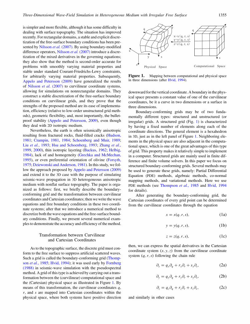
As to the topographic surface, the discrete grid must con-form to the free surface to suppress artificial scattered waves.Such a grid is called the boundary-conforming grid (Thomp-son et al., 1985; Hvid, 1994); it was used early by Fornberg(1988) in seismic-wave simulation with the pseudospectralmethod. A grid of this type is achieved by carrying out a trans-formation between the (curvilinear) computational space andthe (Cartesian) physical space as illustrated in Figure 1. Bymeans of this transformation, the curvilinear coordinates q,r, and s are mapped into Cartesian coordinates within thephysical space, where both systems have positive direction

downward for the vertical coordinate. A boundary in the phys-ical space presents a constant value of one of the curvilinearcoordinates, be it a curve in two dimensions or a surface inthree dimensions.

Boundary-conforming grids may be of two funda-mentally different types: structured and unstructured (orirregular) grids. A structured grid (Fig. 1) is characterizedby having a fixed number of elements along each of thecoordinate directions. The general element is a hexahedronin 3D, just as in the left panel of Figure 1. Neighboring ele-ments in the physical space are also adjacent in the computa-tional space, which is one of the great advantages of this typeof grid. This property makes it relatively simple to implementin a computer. Structured grids are mainly used in finite dif-ference and finite volume solvers. In this paper we focus onstructured boundary-conforming grids. Several methods maybe used to generate these grids, namely: Partial DifferentialEquation (PDE) methods, algebraic methods, co-normalmapping methods, and variational methods. Here we usePDE methods (see Thompson et al., 1985 and Hvid, 1994for details).

After generating the boundary-conforming grid, theCartesian coordinates of every grid point can be determinedfrom the curvilinear coordinates through the equation

x � x�q; r; s�; (1a)

y � y�q; r; s�; (1b)

z � z�q; r; s�; (1c)

then, we can express the spatial derivatives in the Cartesiancoordinate system �x; y; z� from the curvilinear coordinatesystem �q; r; s� following the chain rule

∂x � qx∂q � rx∂r � sx∂s; (2a)

∂y � qy∂q � ry∂r � sy∂s; (2b)

∂z � qz∂q � rz∂r � sz∂s; (2c)

and similarly in other cases

Figure 1. Mapping between computational and physical spacein three dimensions (after Hvid, 1994).

Three-Dimensional Wave-Field Simulation in Heterogeneous Medium with Irregular Free Surface 1355

∂q � xq∂x � yq∂y � zq∂z; (3a)

∂r � xr∂x � yr∂y � zr∂z; (3b)

∂s � xs∂x � ys∂y � zs∂z; (3c)

where qx denotes ∂q�x; y; z�=∂x and the similar in othercases. These derivatives are called metric derivatives orsimply the metric. We can also find the metric derivatives

qx �1

J�yrzs � zrys�; (4a)

qy �1

J�zrxs � xrzs�; (4b)

qz �1

J�xrys � yrxs�; (4c)

rx �1

J�yszq � zsyq�; (4d)

ry �1

J�zsxq � xszq�; (4e)

rz �1

J�xsyq � ysxq�; (4f)

sx �1

J�yqzr � zqyr�; (4g)

sy �1

J�zqxr � xqzr�; (4h)

sz �1

J�xqyr � yqxr�; (4i)

where J is the Jacobian of the transformation that iswritten as

J � xqyrzs � xqyszr � xryqzs

� xryszq � xsyqzr � xsyrzq;

and whose detailed form can be found in Appendix A.It is worth noting that even if the mapping equation (1) is

given by an analytic function, the derivatives should still becalculated numerically to avoid spurious source terms due tothe coefficients of the derivatives when the conservationform of the momentum equations are used (Thompson et al.,1985). In all examples presented in this paper the metricderivatives are computed numerically using second-orderaccurate finite-difference approximations.

Elastic Wave Equations in Cartesian and CurvilinearCoordinate Systems

In the following paragraphs we consider a well-studiedtype of anisotropy in seismology, namely, a transversely iso-tropic medium. In the absence of external force, the elasticwave equations in the Cartesian coordinates are given by

ρ∂2u

∂t2 � ∂∂x

�c11

∂u∂x � c12

∂v∂y� c13

∂w∂z

�� ∂

∂y�c66

∂u∂y

� c66∂v∂x

�� ∂

∂z�c44

∂u∂z � c44

∂w∂x

�; (5a)

ρ∂2v

∂t2 � ∂∂x

�c66

∂v∂x� c66

∂u∂y

�� ∂

∂y�c11

∂v∂y� c12

∂u∂x

� c13∂w∂z

�� ∂

∂z�c44

∂v∂z � c44

∂w∂y

�; (5b)

ρ∂2w

∂t2 � ∂∂x

�c44

∂w∂x � c44

∂u∂z

�� ∂

∂y�c44

∂w∂y � c44

∂v∂z

�

� ∂∂z

�c33

∂w∂z � c13

∂u∂x � c13

∂v∂y

�; (5c)

where cij�x; y; z� are elastic parameters and c66 �0:5�c11 � c12�; u, v, and w are the displacements in x, y, andz directions, respectively; ρ�x; y; z� is density. Equa-tions (5a)–(5c) are complemented by the initial data

u�x; y; z; 0� � u0�x; y; z�; (6a)

v�x; y; z; 0� � v0�x; y; z�; (6b)

w�x; y; z; 0� � w0�x; y; z�; (6c)

∂u�x; y; z; 0�∂t � u1�x; y; z�; (6d)

∂v�x; y; z; 0�∂t � v1�x; y; z�; (6e)

∂w�x; y; z; 0�∂t � w1�x; y; z�: (6f)

Utilizing relationships (2a)–(2c), the wave equa-tions (5a)–(5c) can be rewritten in the curvilinear coordinatesystem in the following form (see Appendix B for details):

1356 H. Lan and Z. Zhang

Jρ∂2u

∂t2 � ∂∂q fJqx�c11�qx∂q � rx∂r � sx∂s�u� c12�qy∂q � ry∂r � sy∂s�v� c13�qz∂q � rz∂r � sz∂s�w�� Jqy�c66�qx∂q � rx∂r � sx∂s�v� c66�qy∂q � ry∂r � sy∂s�u�� Jqz�c44�qz∂q � rz∂r � sz∂s�u� c44�qx∂q � rx∂r � sx∂s�w�g� ∂

∂r fJrx�c11�qx∂q � rx∂r � sx∂s�u� c12�qy∂q � ry∂r � sy∂s�v� c13�qz∂q � rz∂r � sz∂s�w�� Jry�c66�qx∂q � rx∂r � sx∂s�v� c66�qy∂q � ry∂r � sy∂s�u�� Jrz�c44�qz∂q � rz∂r � sz∂s�u� c44�qx∂q � rx∂r � sx∂s�w�g� ∂

∂s fJsx�c11�qx∂q � rx∂r � sx∂s�u� c12�qy∂q � ry∂r � sy∂s�v� c13�qz∂q � rz∂r � sz∂s�w�� Jsy�c66�qx∂q � rx∂r � sx∂s�v� c66�qy∂q � ry∂r � sy∂s�u�� Jsz�c44�qz∂q � rz∂r � sz∂s�u� c44�qx∂q � rx∂r � sx∂s�w�g; (7)

Jρ∂2v

∂t2 � ∂∂q fJqx�c66�qx∂q � rx∂r � sx∂s�v� c66�qy∂q � ry∂r � sy∂s�u�� Jqy�c11�qy∂q � ry∂r � sy∂s�v� c12�qx∂q � rx∂r � sx∂s�u� c13�qz∂q � rz∂r � sz∂s�w�� Jqz�c44�qz∂q � rz∂r � sz∂s�v� c44�qy∂q � ry∂r � sy∂s�w�g� ∂

∂r fJrx�c66�qx∂q � rx∂r � sx∂s�v� c66�qy∂q � ry∂r � sy∂s�u�� Jry�c11�qy∂q � ry∂r � sy∂s�v� c12�qx∂q � rx∂r � sx∂s�u� c13�qz∂q � rz∂r � sz∂s�w�� Jrz�c44�qz∂q � rz∂r � sz∂s�v� c44�qy∂q � ry∂r � sy∂s�w�g� ∂

∂s fJsx�c66�qx∂q � rx∂r � sx∂s�v� c66�qy∂q � ry∂r � sy∂s�u�� Jsy�c11�qy∂q � ry∂r � sy∂s�v� c12�qx∂q � rx∂r � sx∂s�u� c13�qz∂q � rz∂r � sz∂s�w�� Jsz�c44�qz∂q � rz∂r � sz∂s�v� c44�qy∂q � ry∂r � sy∂s�w�g; (8)

Jρ∂2w

∂t2 � ∂∂q fJqx�c44�qz∂q � rz∂r � sz∂s�u� c44�qx∂q � rx∂r � sx∂s�w�� Jqy�c44�qz∂q � rz∂r � sz∂s�v� c44�qy∂q � ry∂r � sy∂s�w�� Jqz�c33�qz∂q � rz∂r � sz∂s�w� c13�qx∂q � rx∂r � sx∂s�u� c13�qy∂q � ry∂r � sy∂s�v�g� ∂

∂r fJrx�c44�qz∂q � rz∂r � sz∂s�u� c44�qx∂q � rx∂r � sx∂s�w�� Jry�c44�qz∂q � rz∂r � sz∂s�v� c44�qy∂q � ry∂r � sy∂s�w�� Jrz�c33�qz∂q � rz∂r � sz∂s�w� c13�qx∂q � rx∂r � sx∂s�u� c13�qy∂q � ry∂r � sy∂s�v�g� ∂

∂s fJsx�c44�qz∂q � rz∂r � sz∂s�u� c44�qx∂q � rx∂r � sx∂s�w�� Jsy�c44�qz∂q � rz∂r � sz∂s�v� c44�qy∂q � ry∂r � sy∂s�w�� Jsz�c33�qz∂q � rz∂r � sz∂s�w� c13�qx∂q � rx∂r � sx∂s�u� c13�qy∂q � ry∂r � sy∂s�v�g: (9)


Free Boundary Conditions in the Cartesian andCurvilinear Coordinate Systems

At the free surface, the boundary conditions in theCartesian coordinates are given by

c11∂u∂x � c12

∂v∂y � c13

∂w∂z c66

∂u∂y � c66

∂v∂x c44

∂u∂z � c44

∂w∂x

c66∂v∂x � c66

∂u∂y c11

∂v∂y � c12

∂u∂x � c13

∂w∂z c44

∂v∂z � c44

∂w∂y

c44∂w∂x � c44

∂u∂z c44

∂w∂y � c44

∂v∂z c33

∂w∂z � c13

∂u∂x � c13

∂v∂y

264

375

nxnynz

24

35 � 0: (10)

Here �nx; ny; nz�T is the inward normal of the free sur-face. Using relationships (2a)–(2c), the boundary conditionsin the curvilinear coordinates of equation (10) can be rewrit-ten as

�sxc11�qxuq � rxur � sxus� � c12�qyvq � ryvr � syvs�� c13�qzwq � rzwr � szws�� sy�c66�qyuq � ryur � syus�� c66�qxvq � rxvr � sxvs�� sz�c44�qzuq � rzur � szus�� c44�qxwq � rxwr � sxws��

� 0; (11)

�sx�c66�qxvq � rxvr � sxvs� � c66�qyuq � ryur � syus�� sy�c11�qyvq � ryvr � syvs�� c12�qxuq � rxur � sxus�� c13�qzwq � rzwr � szws�� sz�c44�qzvq � rzvr � szvs�� c44�qywq � rywr � syws��

� 0; (12)

�sx�c44�qxwq � rxwr � sxws� � c44�qzuq � rzur � szus�� sy�c44�qywq � rywr � syws�� c44�qzvq � rzvr � szvs�� sz�c33�qzwq � rzwr � szws�� c13�qxuq � rxur � sxus�� c13�qyvq � ryvr � syvs��

� 0: (13)

Note that here the normal is represented by the normal-ized metric (evaluated along the free surface)

�sx �sx��

s2x � s2y � s2z

q ; �sy �sy��

s2x � s2y � s2z

q ;

�sz �sz��

s2x � s2y � s2z

q :

A Discretization Scheme on the Curvilinear Grid

To approximate (7)–(9) we discretize the rectangularsolid (Fig. 2)

qi � �i � 1�hq; i � 1;…; Nq; hq � l=�Nq � 1�;rj � �j � 1�hr; j � 1;…; Nr; hr � w=�Nr � 1�;sk � �k � 1�hs; k � 1;…; Ns; hs � h=�Ns � 1�;

(14)

where l, w, and h are the length of the rectangular solid in q,r, and s directions, respectively; hq, hr, and hs > 0 define thegrid size in q, r, and s directions, respectively. The threecomponents of the wave field are given by

�ui;j;k�t�; vi;j;k�t�; wi;j;k�t�� u�qi; rj; sk; t�;v�qi; rj; sk; t�; w�qi; rj; sk; t��;

and the derivation operators are given as

j+1

j

j-1 i-1i+1

ik-1

k+1

k

q

r

s

Figure 2. Grids distributions in curvilinear coordinate. The freesurface is set to be at k � 1 layer, we use the forward difference(Ds�) to approximate the normal derivative in the mixed derivativeson this layer; on other layers, the centered difference scheme (Ds

0)is used.


Dq�ui;j;k �

ui�1;j;k � ui;j;khq

; Dq�ui;j;k � Dq�ui�1;j;k;

Dq0ui;j;k �

1

2�Dq

�ui;j;k �Dq�ui;j;k�;

Dr�ui;j;k �ui;j�1;k � ui;j;k

hr; Dr�ui;j;k � Dr�ui;j�1;k;

Dr0ui;j;k �

1

2�Dr�ui;j;k �Dr�ui;j;k�;

Ds�ui;j;k �ui;j;k�1 � ui;j;k

hs; Ds�ui;j;k � Ds�ui;j;k�1;

Ds0ui;j;k �

1

2�Ds�ui;j;k �Ds�ui;j;k�: (15)

The right-hand sides of equations (7)–(9) contain spatialderivatives of nine basic types, which are discretized accord-ing to the following equations

∂∂q �aωq�≈Dq��Eq

1=2�a�Dq�ω�;

∂∂q �bωr�≈Dq

0�bDr0ω�;

∂∂q �cωs�≈Dq

0�c ~Ds0ω�;

∂∂r �dωq�≈Dr

0�dDq0ω�;

∂∂r �eωr�≈Dr��Er

1=2�e�Dr�ω�;∂∂r �fωs�≈Dr

0�f ~Ds0ω�;

∂∂s �gωq�≈ ~Ds

0�gDq0ω�;

∂∂s �mωr�≈ ~Ds

0�mDr0ω�;

∂∂s �pωs�≈Ds��Es

1=2�p�Ds�ω�: (16)

Here ω represents u, v, or w; a, b, c, d, e, f, g, m, and pare combinations of metric and material coefficients. We in-troduce the following averaging operators

Eq1=2�γi;j;k� � γi�1=2;j;k �

γi;j;k � γi�1;j;k

2;

Er1=2�γi;j;k� � γi;j�1=2;k �

γi;j;k � γi;j�1;k

2;

Es1=2�γi;j;k� � γi;j;k�1=2 �

γi;j;k � γi;j;k�1

2: (17)

The cross terms that contain a normal derivative on theboundary are discretized on one side in the direction normalto the boundary

~Ds0ui;j;k �

�Ds�ui;j;k; k � 1;Ds

0ui;j;k; k ≥ 2:(18)

A Discretization on the Curvilinear Grid: ElasticWave Equations

We approximate the spatial operators in equations (7)–(9) by (16). After suppressing grid indexes, this leads to

Jρ∂2u

∂t2 � Dq��Eq1=2�Mqq

1 �Dq�u� Eq

1=2�Mqq2 �Dq

�v� Eq1=2�Mqq

3 �Dq�w� �Dq

0 �Mqs1

~Ds0u�Mqs

2~Ds0v�Mqs

3~Ds0w�

�Dr0�Mrs

1~Ds0u�Mrs

2~Ds0v�Mrs

3~Ds0w� � ~Ds

0�Msq1 Dq

0u�Msq2 Dq

0v�Msq3 Dq

0w�� ~Ds

0�Msr1 D

r0u�Msr

2 Dr0v�Msr

3 Dr0w� �Dq

0 �Mqr1 Dr

0u�Mqr2 Dr

0v�Mqr3 Dr

0w��Dr

0�Mrq1 Dq

0u�Mrq2 Dq

0v�Mrq3 Dq

0w� �Dr��Er1=2�Mrr

1 �Dr�u� Er1=2�Mrr

2 �Dr�v� Er1=2�Mrr

3 �Dr�w��Ds��Es

1=2�Mss1 �Ds�u� Es

1=2�Mss2 �Ds�v� Es

1=2�Mss3 �Ds�w�≡ L�u��u; v; w�; (19)

Jρ∂2v


5 �Dq�v� Eq

1=2�Mqq2 �Dq

�u� Eq1=2�Mqq


0 �Mqs5

~Ds0v�Msq

2~Ds0u�Mqs

4~Ds0w�

�Dr0�Mrs

5~Ds0v�Msr

2~Ds0u�Mrs

4~Ds0w� � ~Ds

0�Msq5 Dq

0v�Mqs2 Dq

0u�Msq4 Dq

0w�� ~Ds

0�Msr5 D

r0v�Mrs

2 Dr0u�Msr

4 Dr0w� �Dq

0 �Mqr5 Dr

0v�Mrq2 Dr

0u�Mqr4 Dr

0w��Dr

0�Mrq5 Dq

0v�Mqr2 Dq

0u�Mrq4 Dq







1=2�Mss4 �Ds�w�≡ L�v��u; v; w�; (20)


Jρ∂2w


3 �Dq�u� Eq

1=2�Mqq4 �Dq

�v� Eq1=2�Mqq


0 �Msq3

~Ds0u�Msq

4~Ds0v�Mqs

6~Ds0w�

�Dr0�Msr

3~Ds0u�Msr

4~Ds0v�Mrs

6~Ds0w� � ~Ds

0�Mqs3 Dq

0u�Mqs4 Dq

0v�Msq6 Dq

0w�� ~Ds

0�Mrs3 D

r0u�Mrs

4 Dr0v�Msr

6 Dr0w� �Dq

0 �Mrq3 Dr

0u�Mrq4 Dr

0v�Mqr6 Dr

0w��Dr

0�Mqr3 Dq

0u�Mqr4 Dq

0v�Mrq6 Dq







1=2�Mss6 �Ds�w�≡ L�w��u; v; w�; (21)

in the grid points �qi; rj; sk�, �i; j; k�∈�1; Nq� × �1; Nr�×�1; Ns�. We have introduced the following notations forthe material and metric terms in order to express the discre-tized equations in a more compact form:

Mkl1 � Jkxlxc11 � Jkylyc66 � Jkzlzc44;

Mkl2 � Jkxlyc12 � Jkylxc66;

Mkl3 � Jkxlzc13 � Jkzlxc44;

Mkl4 � Jkylzc13 � Jkzlyc44;

Mkl5 � Jkxlxc66 � Jkylyc11 � Jkzlzc44;

Mkl6 � Jkxlxc44 � Jkylyc44 � Jkzlzc33; (22)

where k and l represent the metric coefficients q, r, or s.

We discretize in time using second-order accurate cen-tered differences. The full set of discretized equations is

ρ�un�1 � 2un � un�1

δ2t

�� L�u��un; vn; wn�;

ρ�vn�1 � 2vn � vn�1

δ2t

�� L�v��un; vn; wn�;

ρ�wn�1 � 2wn � wn�1

δ2t

�� L�w��un; vn; wn�; (23)

where δt represents the timestep.

A Discretization on the Curvilinear Grid: FreeBoundary Conditions

The boundary conditions (11)–(13) are discretized by

1

2��Mss

1 �i;j;3=2Ds�ui;j;1 � �Mss1 �i;j;1=2Ds�ui;j;0� � �Msq

1 �i;j;1Dq0ui;j;1 � �Msq

2 �i;j;1Dq0vi;j;1 � �Msq

3 �i;j;1Dq0wi;j;1

� 1

2��Mss

2 �i;j;3=2Ds�vi;j;1 � �Mss2 �i;j;1=2Ds�vi;j;0� � �Msr

1 �i;j;1Dr0ui;j;1 � �Msr

2 �i;j;1Dr0vi;j;1 � �Msr

3 �i;j;1Dr0wi;j;1

� 1

2��Mss

3 �i;j;3=2Ds�wi;j;1 � �Mss3 �i;j;1=2Ds�wi;j;0�

� 0; (24)

1

2��Mss

5 �i;j;3=2Ds�vi;j;1 � �Mss5 �i;j;1=2Ds�vi;j;0� � �Msq

5 �i;j;1Dq0vi;j;1 � �Mqs

2 �i;j;1Dq0ui;j;1 � �Msq

4 �i;j;1Dq0wi;j;1

� 1

2��Mss

2 �i;j;3=2Ds�ui;j;1 � �Mss2 �i;j;1=2Ds�ui;j;0� � �Msr

5 �i;j;1Dr0vi;j;1 � �Mrs

2 �i;j;1Dr0ui;j;1 � �Msr

4 �i;j;1Dr0wi;j;1

� 1

2��Mss


� 0; (25)

1

2��Mss

3 �i;j;3=2Ds�ui;j;1 � �Mss3 �i;j;1=2Ds�ui;j;0� � �Mqs

3 �i;j;1Dq0ui;j;1 � �Mqs

4 �i;j;1Dq0vi;j;1 � �Msq

6 �i;j;1Dq0wi;j;1

� 1

2��Mss

4 �i;j;3=2Ds�vi;j;1 � �Mss4 �i;j;1=2Ds�vi;j;0� � �Mrs

3 �i;j;1Dr0ui;j;1 � �Mrs

4 �i;j;1Dr0vi;j;1 � �Msr

6 �i;j;1Dr0wi;j;1

� 1

2��Mss


� 0; (26)for i � 1;…; Nq; j � 1;…; Nr.


The key step in obtaining a stable explicit discretizationis to use the operator ~Ds

0 (which is one-sided on the bound-ary) for the approximation of the normal derivative in ∂q∂s,∂r∂s, ∂s∂q, and ∂s∂r cross derivatives. At first glance, it mayappear that using a one-sided operator would reduce the ac-curacy of the method to the first order. However, as it wastheoretically shown by Nilsson et al. (2007) (for a Cartesiandiscretization), a first-order error on the boundary in the dif-ferential equations (19)–(21) can be absorbed as a second-order perturbation of the boundary conditions (24)–(26).

In the finite-difference calculations, an artificial reflec-tion arises at the edges of the model domain. To suppress thisspurious reflection, we adopt a combined absorbing bound-ary condition by combing the n-time decoupled absorbingboundary condition (Zhang et al., 1999; Yang et al., 2002;Yang et al., 2003) and exponential damping (Cerjan et al.,1985). In this paper, we choose n � 2, and the detailedderivations and discretization can be found in the earlypapers due to Zhang et al. (1993), Yang (1996), and Heand Zhang (1996).

Accuracy and Efficiency Tests

Accuracy

The accuracy of the proposed method is examined bycomparing the numerical results with the analytical solutionof the Lamb’s problem, first in an isotropic medium and thenin a transversely isotropic case with a vertical symmetry axis(VTI medium).

Analytic Comparison for the Lamb’s Problem in an IsotropicMedium. We choose a half-infinite elastic medium wherethe P velocity is 623 m=s, the S velocity is 360 m=s, and

the density is 1500 kg · m�3 (a Poisson solid). Avertical Rick-er wavelet point source, with a center frequency of 2 Hz (con-taining frequencies up to 6Hz), is loaded at a point 60mbelowthe surface. Thus, in the chosen model of medium, the domi-nant andminimumwavelengths of theSwave areλSdom � 180

and λSmin � 60 m, respectively. The solutions with the gridspacings of 10 and 5m, respectively, are benchmarked againstan analytical solution by H. Zhang and X. Chen (2006). Thenumbers of grid points per shortest shear wavelength for bothof these grid intervals are about 6 and 12, respectively. Wepresent the time-series of the vertical component recorded180, 1080, and 1980 m from the source, that is, records atthe distances of 1, 6, and 11 times the dominant wavelengthfrom the source, respectively (Fig. 3). It can be seen clearlythat the results with 12 grid spacings per minimum wave-length (GSPMW) give much better agreements with theanalytic solutions than those with only 6 GSPMW, and theformer also give a sufficient accuracy in modeling Rayleighwave propagation even for large distances.

In the following, we evaluate the accuracy of the numer-ical method in a quantitative way by using an error criteriondefined by Kristek et al. (2002). The results are given inFigure 4. It can be clearly seen that the results with 12GSPMW give much better amplitudes of Rayleigh waves thanthose with only 6 GSPMW, while both results give goodphases. This is in agreement with the conclusion based onsimple visual comparisons of the seismograms.

Analytic Comparison for the Lamb’s Problem in a VTIMedium. The elastic parameters describing the VTI med-ium are given in Table 1. The analytical solution is obtainedby convolving the free-surface Green’s function with thesource function (Payton, 1983; He and Zhang, 1996). Avertical point source of the type:

−4

−2

0

2

D=λdom

Ver

tical

Dis

plac

emen

t LambModeling (6)

−1.5

−1

−0.5

0

0.5

1

1.5

D=6λdom

LambModeling (6)

−1.5

−1

−0.5

0

0.5

1

D=11λdom

LambModeling (6)

0 2 4 6 8−3

−2

−1

0

1

2

D=λdom

Ver

tical

Dis

plac

emen

t LambModeling (12)

0 2 4 6 8−1

−0.5

0

0.5

D=6λdom

Time (s)

LambModeling (12)

0 2 4 6 8

−0.5

0

0.5

D=11λdom

LambModeling (12)

(a)

(b)

Figure 3. Comparison between numerical and analytical vertical components of the displacement at the epicentral distances ofλSdom, 6λSdom, and 11λSdom, respectively, for the Lamb’s problem in the isotropic medium. Lamb’s result is the analytical solution whilethe modeling result is the numerical solution. Numbers 6 and 12 mean the numbers of the grid spacings per minimum wavelength usedin the numerical calculation.


f�t� � e�0:5f20�t�t0�2 cos πf0�t � t0�; (27)

with t0 � 0:5 s and a high cutoff frequency f0 � 10 Hz, isassumed to be located at the free surface of a 3D half-space(Fig. 5). It should be mentioned that Carcione et al. (1992)and Carcione (2000) presented an analytical comparison ofthe point-source response in a 3D VTI medium in the absenceof the free surface. The comparisons are performed by firsttransforming the 3D numerical results into a line-source re-sponse by carrying out an integration along the receiver line(Wapenaar et al., 1992) and then comparing the emergingresults with the 2D Lamb’s analytical solutions. The numer-ical model contains 401 × 401 × 191 grid nodes in the x, y,and z directions, respectively. The grid spacings are 10 m inall directions. The solution is advanced using a timestep of1.25 ms for 3.5 s.

Three receiver lines are positioned on the free surface,two of which are parallel to the y direction with respectivenormal distances of 130 (Line 1) and 1000 m (Line 2) awayfrom the point source, the other crosses the source locationand parallels the x direction (Line 3). The integrations areperformed along the first two receiver lines; these represent2D results of 130 and 1000 m away from the source, respec-tively. Figure 6 shows the comparisons between the resultingnumerical and 2D analytical z components of the displace-ment for the VTI medium. In spite of the errors resulting fromthe transformation of the point-source response into the line-source one, numerical and analytical results agree well inFigure 6. These comparisons demonstrate the accuracy ofour corresponding algorithm.

Synthetic seismograms are computed at Line 3. Theseismograms in Figure 7 show the direct quasi-P wave (qP)and a high-amplitude Rayleigh wave (R). Snapshots of thevertical component of the wave field in the horizontal (xy)plane at the propagation time of 1.4 s are displayed inFigure 8. We define the incidence plane by the propagationdirection and the z axis, quasi-P wave and quasi-SV wave(qSV) motions lie in this plane, while SH motion is normalto the plane. Hence, the z component does not contain SH

motion. The xy plane of a transversely isotropic medium is aplane of isotropy, where the velocity of the qP wave is about3260 ms�1 and the velocity of the qSV wave is about1528 ms�1. The amplitude of the qP wave is so weak com-pared with that of the Rayleigh and qSV wave that one can

Table 1Medium Parameters in the Homogeneous Half-Space

c11 (GPa) c12 (GPa) c13 (GPa) c33 (GPa) c44 (GPa) ρ (g=cm3)

25.5 2.0 14.0 18.4 5.6 2.4

0 2 4 6 8 10 120.05

0.1

0.15

0.2

0.25

0.3

0.35

0.4

0.45Envelope Misfit

Ver

tical

Dis

plac

emen

t

612

0 2 4 6 8 10 12−1

−0.5

0

0.5

1Phase Misfit

Epicentral distance/dominant wavelength

612

Figure 4. Accuracy of the numerical method for the Lamb’s problem in the isotropic medium. The envelope and phase misfits areevaluated against the normalized epicentral distance. Sampling ratios 6 and 12 are used in the numerical solutions, respectively.

x

yz

Source

Line 1

Line 2

Line 34000 m

4000 m

1900

m

Figure 5. Model of a half-space with a planar free surface. Thesource locates at (300 m, 2000 m) at the surface, which is marked asan asterisk. Three receiver lines (Line 1, Line 2, and Line 3) are alsomarked. Lines 1 and 2 are parallel to the y direction with normaldistances of 130 and 1000 m from the point-source, respectively.Line 3 crosses the source location and lies in the x direction.


hardly identify it in the snapshot (Fig. 8a). In order to observethe qP wave, the amplitude of the wave field is amplified10 times. Owing to this, side reflections also appear in thephoto, as shown in Figure 8b. As the velocity of the Rayleighwave is very close to that of the qSV wave, the two wavesare almost superimposed, and it is difficult to distinguishbetween the two in synthetic seismograms and snapshots.

Figure 9 shows the x-component of the wave field in thevertical (xz) plane at 1.4 and 2.3 s propagation times. The xzplane contains the receiver line (Line 3) and the source loca-tion. Both snapshots show the wave front of the qPwave andthe qSV wave. The former snapshot (1.4 s) shows the qSVwave with the cusps. A headwave (H) can also be found inthe photos; the headwave is a quasi-shear wave and is guidedalong the surface by the qP wave.

Numerical Simulations on an Irregular (Nonflat)Free Surface

Three numerical experiments with irregular free surfacesare now investigated. The first example is a test on smoothboundaries, while the second example consists of a hemi-spherical depression to test the ability of the method for

nonsmooth topography. For the sake of simplicity, bothexamples are based on homogeneous half-spaces, that is, themedium parameters are the same as in the case of a flat sur-face (Table 1). The same source is located at the same placeas in the planar surface model, the timestep is 0.8 ms. Thetotal propagation time is 3.5 s for the two models. Finally, weconsider a two-layered model with a realistic topography.

Topography Simulating a Shaped Gaussian Hill. The firstmodel considered here is a half-space whose free surface is ahill-like feature (Fig. 10). The shape of the hill resembles aGaussian curved surface given by the function

z�x; y� � �150 exp��x � 2000

150

�2

��y � 2000

150

�2�m;

�x; y�∈�0 m; 4000 m�2: (28)

The computational domain extends to depthz�x; y� � 2000 m. The volume is discretized with equal gridnodes in each direction as in the planar surface one. The gridspacings are 10 m in the x and y directions and about 10.5 m

0 0.5 1 1.5 2 2.5 3 3.5−1

−0.5

0

0.5

1

Time (s)

Nor

mal

ized

Ver

tical

Dis

plac

emen

t LambModeling

(a)

D=130 m

0 0.5 1 1.5 2 2.5 3 3.5−1

−0.5

0

0.5

1

Time (s)

Nor

mal

ized

Ver

tical

Dis

plac

emen

t LambModeling

(b)

D=1000 m

Figure 6. Comparison between numerical and analytical vertical components of the displacement for the Lamb’s problem in the VTImedium: (a) Line 1 parallels the y direction, at normal distance of 130 m from the energy source (Fig. 5); (b) Line 2 parallels the y direction, atnormal distance of 1000 m from the energy source. Lamb’s result is an analytical solution of the 2D Lamb’s problem of the VTI medium. Themodeling result is the line-source response of the 3D VTI medium obtained by the superposition of the 3D point-source responses. A goodagreement is observed.

Figure 7. Seismograms along Line 3 that cross the source loca-tion and are parallel to the x direction (Fig. 5), for the planar surfacemodel: (a) x-component (horizontal) of the displacement; (b) z-component (vertical). Symbol qP indicates the qP wave; R indi-cates Rayleigh wave.

Figure 8. Snapshots of the vertical component of the wave fieldat the surface (xy plane) of the planar surface model. The amplitudeof the wave field in (b) is 10 times enlarged compared with (a). Thequasi-P wave (qP), Rayleigh wave (R), and side reflections aremarked (SR).


in the z direction for average. The vertical spacing varies withdepth; it is smaller toward the free surface and larger towardthe bottom of the model. The minimum and maximum of thevertical spacings are 6 and 12 m, respectively.

The gridding scheme that shows the detailed crosssection of the grids along Line 3 is shown in Figure 11.Synthetic seismograms are also computed at Line 3 (Fig. 12).As a result of the hill-shaped free surface (and compared withthe synthetic seismograms in Figure 7), the amplitudes of thequasi-Pwave and Rayleigh wave are reduced in the right partof the sections. In addition, after the ordinary quasi-P wave asecondary quasi-P wave (RqPf) induced by the scattering ofthe direct Rayleigh wave can be observed. Similarly, asecondary Rayleigh wave (qPRf) that travels in front of theordinary Rayleigh wave induced by the scattering of thedirect quasi-P wave can also be distinguished. Some energyis scattered back to the left side as a Rayleigh wave (qPRb,RR) and a quasi-P wave (RqPb).

Snapshots of thewave field in the horizontal (xy) plane atdifferent propagation times are displayed in Figure 13. Theamplitudes are 10 times enlarged. In the beginning the wavefield propagates undisturbed along the free surface. At 1.1 sthe direct quasi-P wave hits the hill and generates a circular

diffracted wave. This wave is a Rayleigh wave, which ismarked as two parts: one travels forward (qPRf) and the othertravels backward (qPRb). These can be seen clearly in thelater snapshots (1.4–2.3 s). In addition, a reflected Rayleighwave (RR) can be observed. The direct quasi-Pwave (qP) andRayleigh wave (R) are also marked in the figure. By the way,side reflections from the boundaries can also be noted in theplane. Figure 14 shows the x component of the wave field inthe vertical (xz) plane. The xz plane contains the receiverline and source location. The snapshots show the diffractedquasi-P and quasi-SV waves clearly in the vertical plane.

Topography Simulating a Shaped Hemispherical Depres-sion. In the second model, we consider a hemisphericaldepression model as illustrated in Figure 15. The first modelthat we have considered is of smooth topography, that is, withcontinuous and finite slopes everywhere. However, theshaped hemispherical depression here taken as a reference isa case of extreme topography, such that the vertical-to-horizontal ratio of the depression is very large (1∶2) andthe slopes of the edges tend to infinity. The hemispherical

Figure 9. Snapshots of the x component of the wave field in thevertical (xz) plane that contains the receiver line and the source at(a) 1.4 s and (b) 2.3 s propagation times for the planar surface mod-el. The quasi-P wave (qP), quasi-SV wave (qSV), and a head wave(H) generated at the free surface are marked.

Source

x

yz

Line 3

4000 m

4000 m

2000

m

Figure 10. Model of a half-space with Gaussian shape hill to-pography. The size of the model is 4000 m × 4000 m × 2000 m.The source locates at (300 m, 2000 m) at the surface, which ismarked as an asterisk. The receiver line (Line 3) crossing the sourcelocation and lying in the x direction is also marked.

Figure 11. The gridding scheme that shows the detailed crosssection of the grids along Line 3 in the Gaussian shape hill topo-graphy model. For clarity, the grids are displayed with a reducingdensity factor of 3.

Figure 12. Seismograms along the receiver line for the Gaus-sian shape hill topography model: (a) x component (horizontal) ofthe displacement; (b) z component (vertical). Symbols are: qPd: qPwave diffracts to qPwave; Rd: Rayleigh wave diffracts to Rayleighwave; qPRf: qP wave scatters to Rayleigh wave and propagatesforward; qPRb: qP wave scatters to Rayleigh wave and propagatesbackward; RqPf: Rayleigh wave scatters to qP wave and propa-gates forward; RqPb: Rayleigh wave scatters to qP wave and pro-pagates backward; RR: Rayleigh wave reflects to Rayleigh wave.


depression is at the middle of the free surface, and the radiusis 150 m.

The numerical model is discretized in the same way as inthe hill topography model. The gridding scheme that showsthe detailed cross section of the grids along Line 3 is shownin Figure 16. Owing to the existence of model edges withstrong slopes at x � 1850 and x � 2150 m along the recei-ver line, both body waves and Rayleigh waves scattered bysharp changes in the topography can be clearly observed onthe synthetic seismograms shown in Figure 17. Owing to itsshorter wavelength, the scattering of Rayleigh waves is muchstronger than that of the body waves when propagatingthrough the hemispherical depression, thus indicating thatsuch sharp depression can affect the propagation of Rayleighwaves significantly.

The photos in Figure 18 show the vertical component ofthe wave field in the horizontal (xy) plane. Compared with

the photos of the hill topography model, we can see theRayleigh wave scattering at the edges of the hemisphericaldepression; it seems as if the reflected Rayleigh wave pro-pagates faster in the hemispherical depression model than inthe hill topography model. What’s more, the back-scattered

Figure 13. Snapshots of the vertical component of the wavefield at the surface (xy plane) at different propagation times forthe Gaussian shape hill topography model. To see the scatteredwaves especially the scatterings from the qP wave clearly, the am-plitudes of the wave field have been amplified 10 times. Side reflec-tions from the boundaries also appear in the photos (SR). Symbolsare: qP: the qP wave; R: the Rayleigh wave; qPRf: qP wave scat-ters to Rayleigh wave and propagates forward; qPRb: qP wavescatters to Rayleigh wave and propagates backward; RR: Rayleighwave reflects to Rayleigh wave.

Figure 14. Snapshots of the x component of the wave field inthe vertical (xz) plane that contains the receiver line and the sourceat different propagation times for the Gaussian shape hill topogra-phy model.

x

yz

Line3

Source

4000 m

4000 m

20

00

m

Figure 15. Model of a half-space with hemispherical shapedepression topography. The size of the model is 4000 m×4000 m × 2000 m. The source locates at (300 m, 2000 m) at thesurface, which is marked as an asterisk. The receiver line (Line3) crossing the source location and lying in the x direction is alsomarked.


waves of Rayleigh wave in the hemispherical depressionmodel are much stronger; this may also indicate that suchsharp depression blocks the propagation of Rayleigh wavemore significantly.

Real Topography Simulating. It is also interesting to studya realistic example. We consider a model in Tibet (Fig. 19).The length and width of the model are 21.6 km, and the aver-age height of the topography is roughly�3560 m (3560 m inthe geodetic coordinate system). The digital elevation dataset is provided by International Scientific & Technical DataMirror Site, Computer Network Information Center, ChineseAcademy of Sciences (see the Data and Resources section).The computational domain is extended to depth z�x; y� �7200 m. For simplicity we use a two-layered model withparameters given in the model sketch (Fig. 19) instead ofthe real velocity structure under the realistic topography.It consists of 241 × 241 × 121 grid nodes in the x, y, andz directions, respectively, with equal vertical grid nodes ineach layer. A vertical point source such as the one used inprevious models is loaded in the middle of the free surface,

where the high cutoff frequency has been changed to 2.7 Hzand the time-shift is 1.5 s. Two lines of receivers crossing thesource location and paralleling the x and y directions, respec-tively, are placed at the free surface. The timestep is 5 ms,and the total propagation time is 8 s.

Snapshots of the z component of the wave field in thevertical plane that contains receiver Line 1 and the sourcelocation are presented on Figure 20, and the seismogramsof the z component are also computed at the two receiverlines (Fig. 21). We can see that the effect of the topographyis very important, with strong scattered phases that are super-imposed to the direct and reflected waves, which make itvery difficult to identify effective reflections from subsurfaceinterface. The scattering in the seismograms also reflect dif-ferent features of the surface. The scattering in the seismo-grams at Line 1 (Fig. 21a) is much stronger than in theseismogram at Line 2 (Fig. 21b), indicating that the surfacealong Line 1 is much rougher than along Line 2, which also

Figure 16. The gridding scheme that shows the detailed crosssection of the grids along Line 3 in the hemispherical shape depres-sion topography model. For clarity, the grids are displayed with areducing density factor of 3.

Figure 17. Seismograms at the receiver line for the hemisphe-rical shape depression topography model: (a) x component (hori-zontal) of the displacement; (b) z component (vertical). Symbolsare: qPd: qP wave diffracts to qP wave; Rd: Rayleigh wave dif-fracts to Rayleigh wave; qPRf: qP wave scatters to Rayleigh waveand propagates forward; qPRb: qP wave scatters to Rayleigh waveand propagates backward; RqPf: Rayleigh wave scatters to qPwave and propagates forward; RqPb: Rayleigh wave scatters toqP wave and propagates backward; RR: Rayleigh wave reflectsto Rayleigh wave.

Figure 18. Snapshots of the vertical component of the wavefield at the surface (xy plane) at different propagation times forthe hemispherical shape depression topography model. To seethe scattered waves especially the scatterings from the qP waveclearly, the amplitudes of the wave field have been amplified10 times. Side reflections from the boundaries also appear in thephotos (SR). Symbols are: qP: the qP wave; R: the Rayleigh wave;qPRf: qP wave scatters to Rayleigh wave and propagates forward;qPRb: qP wave scatters to Rayleigh wave and propagates back-ward; RR: Rayleigh wave reflects to Rayleigh wave.


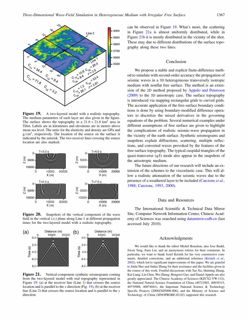
can be observed in Figure 19. What’s more, the scatteringin Figure 21a is almost uniformly distributed, while inFigure 21b it is mostly distributed in the vicinity of the shot.These may due to different distributions of the surface topo-graphy along these two lines.

Conclusion

We propose a stable and explicit finite-difference meth-od to simulate with second-order accuracy the propagation ofseismic waves in a 3D heterogeneous transversely isotropicmedium with nonflat free surface. The method is an exten-sion of the 2D method proposed by Appelo and Petersson(2009) to the 3D anisotropic case. The surface topographyis introduced via mapping rectangular grids to curved grids.The accurate application of the free-surface boundary condi-tions is done by using boundary-modified difference opera-tors to discretize the mixed derivatives in the governingequations of the problem. Several numerical examples underdifferent assumptions of free surface are given to highlightthe complications of realistic seismic-wave propagation inthe vicinity of the earth surface. Synthetic seismograms andsnapshots explain diffractions, scattering, multiple reflec-tions, and converted waves provoked by the features of thefree-surface topography. The typical cuspidal triangles of thequasi-transverse (qS) mode also appear in the snapshots ofthe anisotropic medium.

The future directions of our research will include an ex-tension of the schemes to the viscoelastic case. This will al-low a realistic attenuation of the seismic waves due to thepresence of a weathered layer to be included (Carcione et al.,1988; Carcione, 1993, 2000).

Data and Resources

The International Scientific & Technical Data MirrorSite, Computer Network Information Center, Chinese Acad-emy of Sciences was searched using datamirror.csdb.cn (lastaccessed July 2010).

Acknowledgments

We would like to thank the editor Michel Bouchon, also Jose Badal,Jiwen Teng, Enru Liu, and an anonymous referee for their comments. Inparticular, we want to thank Jozef Kristek for his very constructive com-ments, detailed corrections, and an additional reference (Kristek et al.,2002), which led to significant improvements of this paper. We are gratefulto Jinlai Hao and Jinhai Zhang for their assistance and the facilities given inthe course of this work. Fruitful discussions with Tao Xu, Haiming Zhang,Kai Liang, Lin Chen, Wei Zhang, Hongwei Gao, and Daniel Appelo are alsogreatly appreciated. The Chinese Academy of Sciences (KZCX2-YW-132),the National Natural Science Foundation of China (40721003, 40830315,40739908, 40874041), the Important National Science & TechnologySpecific Projects (2008ZX05008-006), and the Ministry of Science andTechnology of China (SINOPROBE-02-02) supported this research.

Figure 19. A two-layered model with a realistic topography.The medium parameters of each layer are also given in the figure.The surface shows the topography in a 21:6 × 21:6 km2 area inTibet. Labels are in kilometers and elevations are in meters abovemean sea level. The units for the elasticity and density are GPa andg=cm3, respectively. The location of the source on the surface isindicated by the asterisk. The two receiver lines crossing the sourcelocation are also marked.

Figure 20. Snapshots of the vertical component of the wavefield in the vertical (xz) plane along Line 1 at different propagationtimes for the two-layered model with a realistic topography.

Figure 21. Vertical-component synthetic seismograms comingfrom the two-layered model with real topography represented inFigure 19: (a) at the receiver line (Line 1) that crosses the sourcelocation and is parallel to the x direction (Fig. 19); (b) at the receiverline (Line 2) that crosses the source location and is parallel to the ydirection.


http://datamirror.csdb.cn



References

Al-Shukri, H. J., G. L. Pavlis, and F. L. Vernon III(1995). Site effectobservations from broadband arrays, Bull. Seismol. Soc. Am. 85,1758–1769.

Appelo, D., and N. A. Petersson (2009). A stable finite difference method forthe elastic wave equation on complex geometries with free surfaces,Commun. Comput. Phys. 5, 84–107.

Ashford, S. A., N. Sitar, J. Lysmer, and N. Deng (1997). Topographic effectson the seismic response of steep slopes, Bull. Seismol. Soc. Am. 87,701–709.

Backus, G. E. (1962). Long-wave elastic anisotropy produced by horizontallayering, J. Geophys. Res. 67, 4427–4440.

Boore, D. M. (1972). A note on the effect of simple topography on seismicSH waves, Bull. Seismol. Soc. Am. 62, 275–284.

Bouchon, M., M. Campillo, and S. Gaffet (1989). A boundary integral equa-tion-discrete wavenumber representation method to study wave propa-gation in multilayered medium having irregular interfaces, Geophysics54, 1134–1140.

Bouchon, M., C. A. Schultz, and M. N. Toksoz (1995). A fast implementa-tion of boundary integral equation methods to calculate the propaga-tion of seismic waves in laterally varying layered medium, Bull.Seismol. Soc. Am. 85, 1679–1687.

Campillo, M. (1987). Modeling of SH wave propagation in an irregularlylayered medium. Application to seismic profiles near a dome, Geo-phys. Prospecting 35, 236–249.

Campillo, M., and M. Bouchon (1985). Synthetic SH seismograms in a lat-erally varying medium by the discrete wavenumber method, Geophys.J. R. Astr. Soc. 83, 307–317.

Carcione, J. M. (1993). Seismic modeling in viscoelastic medium,Geophysics 58, 110–120.

Carcione, J. M. (2000). Wave Fields in Real Medium: Wave Propagationin Anisotropic, Anelastic and Porous Medium, Pergamon,Amsterdam.

Carcione, J. M., D. Kosloff, A. Behle, and G. Seriani (1992). A spectralscheme for wave propagation simulation in 3-D elastic-anisotropicmedium, Geophysics 57, 1593–1607.

Carcione, J. M., D. Kosloff, and R. Kosloff (1988). Viscoacoustic wave pro-pagation simulation in the earth, Geophysics 53, 769–777.

Cerjan, C., D. Kosloff, R. Kosloff, and M. Reshef (1985). A nonreflectingboundary condition for discrete acoustic and elastic wave equations,Geophysics 50, 705–708.

Crampin, S. (1981). A review of wave motion in anisotropic and crackedelastic-medium, Wave Motion 3, 343–391.

Crampin, S. (1984). Effective anisotropic elastic constants for wave propa-gation through cracked solids, Geophys. J. Int. 76, 135–145.

Durand, S., S. Gaffet, and J. Virieux (1999). Seismic diffracted waves fromtopography using 3-D discrete wavenumber-boundary integral equa-tion simulation, Geophysics 64, 572–578.

Dziewonski, A. M., and D. L. Anderson (1981). Preliminary reference Earthmodel, Phys. Earth Planet. In. 25, 297–356.

Fornberg, B. (1988). The pseudo-spectral method: Accurate representationin elastic wave calculations, Geophysics 53, 625–637.

Forsyth, D. W. (1975). The early structural evolution and anisotropy of theoceanic upper mantle, Geophys. J. Int. 43, 103–162.

Frankel, A. (1993). Three-dimensional simulations of ground motion in theSan Bernardino Valley, California, for hypothetical earthquakes on theSan Andreas fault, Bull. Seismol. Soc. Am. 83, 1020–1041.

Frankel, A., and J. Vidale (1992). A three-dimensional simulation of seismicwaves in the Santa Clara Valley, California, from a Loma Prieta after-shock, Bull. Seismol. Soc. Am. 82, 2045–2074.

Galis, M., P. Moczo, and J. Kristek (2008). A 3-D hybrid finite-difference—Finite-element viscoelastic modelling of seismic wave motion,Geophys. J. Int. 175, 153–184.

Gao, H., and J. Zhang (2006). Parallel 3-D simulation of seismic wavepropagation in heterogeneous anisotropic medium: A grid methodapproach, Geophys. J. Int. 165, 875–888.

Grechka, V. Y., and G. A. McMechan (1995). Is shear-wave splitting an in-dicator of seismic anisotropy?, SEG Expanded Abstracts 14, 332–335.

Hayashi, K., D. R. Burns, and M. N. Toksoz (2001). Discontinuous-gridfinite-difference seismic modeling including surface topography, Bull.Seismol. Soc. Am. 91, 1750–1764.

He, Q., and Z. Zhang (1996). Seismic Propagation and NumericalSimulation in Transversely Isotropic Medium, Jilin University Press(in Chinese).

Helbig, K. (1984). Anisotropy and dispersion in periodically layeredmedium, Geophysics 49, 364–373.

Hestholm, S. (2003). Elastic wave modeling with free surfaces: Stability oflong simulations, Geophysics 68, 314–321.

Hestholm, S., and B. Ruud (1994). 2-D finite-difference elastic wavemodeling including surface topography, Geophys. Prosp. 42,371–390.

Hestholm, S., and B. Ruud (1998). 3-D finite-difference elastic wavemodeling including surface topography, Geophysics 63, 613–622.

Hestholm, S. O., B. O. Ruud, and E. S. Husebye (1999). 3-D versus 2-Dfinite-difference seismic synthetics including real surface topography,Phys. Earth Planet. Inter. 113, 339–354.

Hsu, C. J., and M. Schoenberg (1993). Elastic waves through a simulatedfractured medium, Geophysics 58, 964–977.

Hudson, J. A. (1981). Wave speeds and attenuation of elastic waves inmaterial containing cracks, Geophys. J. Int. 64, 133–150.

Hvid, S. L. (1994). Three dimensional algebraic grid generation, Ph.D.Thesis, Technical University of Denmark.

Jih, R. S., K. L. McLaughlin, and Z. A. Der (1988). Free-boundary condi-tions of arbitrary polygonal topography in a two-dimensional explicitelastic finite-difference scheme, Geophysics 53, 1045.

Komatitsch, D., and J. Tromp (1999). Introduction to the spectral elementmethod for three-dimensional seismic wave propagation, Geophys.J. Int. 139, 806–822.

Komatitsch, D., and J. Tromp (2002). Spectral-element simulations ofglobal seismic wave propagation-I. Validation, Geophys. J. Int. 149,390–412.

Komatitsch, D., and J. P. Vilotte (1998). The spectral element method: anefficient tool to simulate the seismic response of 2D and 3D geologicalstructures, Bull. Seismol. Soc. Am. 88, 368–392.

Kristek, J., P. Moczo, and R. J. Archuleta (2002). Efficient methods tosimulate planar free surface in the 3D fourth-order staggered-gridfinite-difference schemes, Studia Geophys. Geod. 46, no. 2,355–381.

Levander, A. R. (1990). Seismic scattering near the earth’s surface, PureAppl. Geophys. 132, 21–47.

Liu, E., and Z. Zhang (2001). Numerical study of elastic wave scattering bycracks or inclusions using the boundary integral equation method,J. Comput. Acoust. 9, 1039–1054.

Liu, E., S. Crampin, J. H. Queen, and W. D. Rizer (1993). Velocity andattenuation anisotropy caused by microcracks and microfractures ina multiazimuth reverse VSP, Can. J. Explor. Geophys. 29, 177–188.

Liu, E., Z. Zhang, J. Yue, and A. Dobson (2008). Boundary integral model-ling of elastic wave propagation in multi-layered 2D medium withirregular interfaces, Commun. Comput. Phys. 3, no. 1, 52–62.

Lombard, B., J. Piraux, C. Gélis, and J. Virieux (2008). Free and smoothboundaries in 2-D finite-difference schemes for transient elastic waves,Geophys. J. Int. 172, 252–261.

Moczo, P., E. Bystricky, J. Kristek, J. Carcione, and M. Bouchon (1997).Hybrid modelling of P-SV seismic motion at inhomogeneous viscoe-lastic topographic structures, Bull. Seismol. Soc. Am. 87, 1305–1323.

Nielsen, P., F. If, P. Berg, and O. Skovgaard (1994). Using the pseudo-spectral technique on curved grids for 2D acoustic forward modelling,Geophys. Prospect. 42, 321–342.

Nilsson, S., N. A. Petersson, B. Sjogreen, and H. O. Kreiss (2007). Stabledifference approximations for the elastic wave equation in secondorder formulation, SIAM J. Numer. Anal. 45, 1902–1936.

Oprsal, I., and J. Zahradník (1999). Elastic finite-difference method forirregular grids, Geophysics 64, 240–250.


Payton, R. G. (1983). Elastic Wave Propagation in Transversely IsotropicMedium, Martinus Nijhoff Publishers.

Rial, J. A., N. G. Saltzman, and H. Ling (1992). Earthquake-inducedresonance in sedimentary basins, American Scientist 80, 566–578.

Robertsson, J. O. A. (1996). A numerical free-surface condition for elastic/viscoelastic finite-difference modeling in the presence of topography,Geophysics 61, 1921–1934.

Robertsson, J. O. A., and K. Holliger (1997). Modeling of seismic wavepropagation near the earth’s surface, Phys. Earth Planet. Inter. 104,193–211.

Sánchez-Sesma, F. J., and M. Campillo (1991). Diffraction of P, SV, andRayleigh waves by topographic features: A boundary integral formu-lation, Bull. Seismol. Soc. Am. 81, 2234–2253.

Sánchez-Sesma, F. J., and M. Campillo (1993). Topographic effectsfor incident P, SV and Rayleigh waves, Tectonophysics 218,113–125.

Sánchez-Sesma, F. J., M. A. Bravo, and I. Herrera (1985). Surface motion oftopographical irregularities for incident P, SV, and Rayleigh waves,Bull. Seismol. Soc. Am. 75, 263–269.

Sánchez-Sesma, F. J., J. Ramos-Martínez, and M. Campillo (1993). Anindirect boundary element method applied to simulate the seismicresponse of alluvial valleys for incident P, S and Rayleigh waves,Earthquake Eng. Struct. Dynam. 22, 279–295.

Schoenberg, M., and F. Muir (1989). A calculus for finely layered anisotro-pic medium, Geophysics 54, 581–589.

Tessmer, E., and D. Kosloff (1994). 3-D elastic modeling with surfacetopography by a Chebychev spectral method, Geophysics 59,464–473.

Tessmer, E., D. Kosloff, and A. Behle (1992). Elastic wave propagationsimulation in the presence of surface topography, Geophys. J. Int.108, 621–632.

Thompson, J. F., Z. U. A. Warsi, and C. W. Mastin (1985). NumericalGrid Generation: Foundations and Applications, North-holland,Amsterdam.

Toshinawa, T., and T. Ohmachi (1992). Love wave propagation in athree-dimensional sedimentary basin, Bull. Seismol. Soc. Am. 82,1661–1667.

Wapenaar, C., D. Verschuur, and P. Herrmann (1992). Amplitude preproces-sing of single and multicomponent seismic data, Geophysics 57,1178–1188.

Wong, H. L. (1982). Effect of surface topography on the diffraction of P, SV,and Rayleigh waves, Bull. Seismol. Soc. Am. 72, 1167–1183.

Yang, D. (1996). Forward simulation and inversion of seismic waveequations in anisotropic medium, Ph.D. Dissertation, Institute ofGeophysics, Chinese Academy of Sciences.

Yang, D. H., E. Liu, Z. J. Zhang, and J. Teng (2002). Finite-difference mod-elling in two-dimensional anisotropic medium using a flux-correctedtransport technique, Geophys. J. Int. 148, 320–328.

Yang, D., S. Wang, Z. Zhang, and J. Teng (2003). n-Times absorbing bound-ary conditions for compact finite-difference modeling of acoustic andelastic wave propagation in the 2D TI medium, Bull. Seismol. Soc. Am.93, 2389–2401.

Zhang, H., and X. Chen (2006). Dynamic rupture on a planar fault inthree-dimensional half-space—I. Theory, Geophys. J. Int. 164, no. 3,633–652.

Zhang, W., and X. Chen (2006). Traction image method for irregular freesurface boundaries in finite difference seismic wave simulation,Geophys. J. Int. 167, 337–353.

Zhang, Z., and S. L. Klemperer (2010). Crustal structure of the TethyanHimalaya, south Tibet: New constraints from old wide-angle seismicdata, Geophys. J. Int. 181, 1247–1260.

Zhang, Z., Q. He, and Z. Xu (1993). Absorbing boundary condition for FDmodeling in 2D inhomogeneous TIM, Chin. J. Geophys. 36, no. 6,519–527.

Zhang, Z., J. Teng, and Z. He (2000). Azimuthal anisotropy of seismicvelocity, attenuation and Q value in viscous EDA medium, Sci. ChinaE 43, 17–22.

Zhang, Z., G. Wang, and J. M. Harris (1999). Multi-component wavefieldsimulation in viscous extensively dilatancy anisotropic medium, Phys.Earth Planet. Inter. 114, 25–38.

Zhang, Z., X. Yuan, Y. Chen, X. Tian, R. Kind, X. Li, and J. Teng (2010).Seismic signature of the collision between the east Tibetan escape flowand the Sichuan Basin, Earth Planet Sci Lett. 292, 254–264.

Appendix A

Partial Derivatives and Jacobian

In the Transformation between Curvilinear and Carte-sian Coordinates section, the formulation involves the partialderivatives ∂q=∂x, ∂q=∂y, ∂q=∂z, ∂r=∂x, ∂r=∂y, ∂r=∂z,∂s=∂x, ∂s=∂y, ∂s=∂z. They can be found from

ai � ∇ξi � 1

J�aj × ak�; �i � 1; 2; 3�;

�i; j; k�cyclic;(A1)

where ai (i � 1, 2, 3) are the three contravariant base vectorsof the curvilinear coordinate system, where the three curvi-linear coordinates are represented by ξi (i � 1, 2, 3), that is,q, r, and s in this paper. The contravariant base vectors arenormal to the three coordinate surfaces. ai (i � 1, 2, 3) arethe three covariant base vectors of the curvilinear coordinatesystem, and the subscript i in ai indicates the base vectorcorresponding to the ξi coordinate, that is, the tangent tothe coordinate line along which only ξi varies. The covariantbase vectors can be expressed in the form

ai � xξi i� yξi j� zξik; �i � 1; 2; 3�; (A2)

that is,

a1 � xqi� yqj� zqk; (A3)

a2 � xri� yrj� zr; (A4)

a3 � xsi� ysj� zsk; (A5)

where i, j, and k are unit vectors in the x, y, and z directions,respectively. J is the Jacobian of the transformation and isgiven by

J ��xq xr xsyq yr yszq zr zs

��: (A6)

Equation (A1) can be written in a more explicit form

a1 � ∇q � qxi� qyj� qzk � 1

Ja2 × a3; (A7)

a2 � ∇r � rxi� ryj� rzk � 1

Ja3 × a1; (A8)


a3 � ∇s � sxi� syj� szk � 1

Ja1 × a2: (A9)

After using equations (A3)–(A5) to substitute the covar-iant base vectors in equations (A7)–(A9), we can get theexpression (4).

Appendix B

Conservative Form of the Momentum Equations

For 3D inhomogeneous, linear, anisotropic elastic med-ium, the tensor form of the second-order partial differentialdisplacement-stress equations consist of the momentumconservation equation

ρ∂2u∂t2 � ∇ · σ; (B1)

and the generalized Hook’s Law

σkl � cijklεij; (B2)

where i, j, k, l � x, y, z. In curvilinear coordinates, theoperator ∇ · A can be expressed in two forms (Thompsonet al., 1985), namely: the conservative form

∇ · A � 1

J

X3i�1

�Jai · A�ξi ; (B3)

and the nonconservative form

∇ · A �X3i�1

ai · Aξi ; (B4)

where ξi∈fq; r; sg, J is the Jacobian of the transformation,and ai (i � 1, 2, 3) are the contravariant base vectors, whichcan be found in Appendix A. Substituting the conservativeform of the operator ∇ into the momentum conservationequation (5a)–(5c), we can deduce the conservative formof the momentum equation in curvilinear coordinates asequations (7)–(9).

State Key Laboratory of Lithosphere EvolutionInstitute of Geology and GeophysicsChinese Academy of SciencesBeijing, 100029, PR [email protected]

Manuscript received 15 July 2010


Documents

by Haiqiang Lan and Zhongjie Zhang