Embed Size (px)
Citation preview

1
MIXED FORMULATION USING IMPLICIT BOUNDARY FINITE ELEMENT METHOD
By
HAILONG CHEN
A THESIS PRESENTED TO THE GRADUATE SCHOOL OF THE UNIVERSITY OF FLORIDA IN PARTIAL FULFILLMENT
OF THE REQUIREMENTS FOR THE DEGREE OF MASTER OF SCIENCE
UNIVERSITY OF FLORIDA
2012

2
© 2012 Hailong Chen

3
To my parents and wife

4
ACKNOWLEDGMENTS
I would like to express my gratitude to my advisor and chairman of my supervisory
committee, Prof. Ashok V. Kumar, for his guidance, enthusiasm and constant support
throughout my master’s research. I would like to thank him for the numerous insights he
provided during every stage of the research. Without his assistance it would not have
been possible to complete this thesis.
I would like to thank the members of my advisory committee, Prof. Loc Vu-Quoc
and Prof. Bhavani V. Sankar. I’m grateful for their willingness to serve on my committee,
for providing help whenever required, for reviewing this thesis and valuable suggestions
provided.
I would like to thank my undergraduate mentor, Na Li, for her numerous
encouragement and support during my undergraduate study in China and graduate
study in University of Florida, US.
I would like to thank my wife and parents, for their constant love and support
without which this would not have been possible.

5
TABLE OF CONTENTS page
ACKNOWLEDGMENTS .................................................................................................. 4
LIST OF TABLES ............................................................................................................ 8
LIST OF FIGURES ........................................................................................................ 10
LIST OF ABBREVIATIONS ........................................................................................... 14
ABSTRACT ................................................................................................................... 15
CHAPTER
1 INTRODUCTION .................................................................................................... 17
1.1 Overview ........................................................................................................... 17
1.2 Goals and Objectives ........................................................................................ 19 1.3 Outlines ............................................................................................................. 19
2 MESHLESS AND MESH INDEPENDENT METHOD ............................................. 21
2.1 Traditional FEM ................................................................................................ 21
2.2 Meshless and Mesh Independent Method ........................................................ 22
2.3 Implicit Boundary Finite Element Method .......................................................... 23
3 MIXED FORMULATION FOR NEARLY INCOMPRESSIBLE MEDIA .................... 26
3.1 Overview ........................................................................................................... 26 3.2 Mixed Formulation ............................................................................................ 27
3.2.1 Matrix Decomposition .............................................................................. 27
3.2.2 Weak Form .............................................................................................. 29 3.3 2D Plane Strain ................................................................................................. 33
3.4 3D Stress .......................................................................................................... 35 3.5 Numerical Examples and Results ..................................................................... 38
3.5.1 Bracket (Plane strain) .............................................................................. 38 3.5.2 Beam (3D stress)..................................................................................... 39
3.6 Concluding Remarks ......................................................................................... 39
4 CLASSICAL PLATE THEORIES ............................................................................ 43
4.1 Overview ........................................................................................................... 43
4.2 Classical (Kirchhoff) Plate Theory (CPT) .......................................................... 44 4.2.1 Assumptions ............................................................................................ 44 4.2.2 Strain-displacement Relationship ............................................................ 45 4.2.3 Governing Equations ............................................................................... 46

6
4.3 Mindlin Plate Theory (First-order Shear Deformation Theory) (FSDT) .............. 46 4.3.1 Assumptions ............................................................................................ 46 4.3.2 Strain-displacement Relationship ............................................................ 47
4.3.3 Governing Equations ............................................................................... 48 4.3.4 Constitutive Relationship ......................................................................... 51
4.4 Analytical and Exact Solution ............................................................................ 52 4.4.1 Cantilever Plate ....................................................................................... 53 4.4.2 Square Plate ............................................................................................ 54
4.4.3 Circular Plate ........................................................................................... 58 4.4.4 30-degree Skew Plate ............................................................................. 60 4.4.5 60-degree Skew Plate ............................................................................. 61
5 MIXED FORMULATION FOR MINDLIN PLATE ..................................................... 66
5.1 Mixed Form ....................................................................................................... 66 5.2 Discrete Collocation Constraints Method .......................................................... 69
5.3 Applying EBC Using Implicit Boundary Method ................................................ 73 5.4 Numerical Results ............................................................................................. 78
5.4.1 Cantilever Plate ....................................................................................... 78 5.4.2 Square Plate ............................................................................................ 79 5.4.3 Circular Plate ........................................................................................... 79
5.4.4 30-degree Skew Plate ............................................................................. 80 5.4.5 60-degree Skew Plate ............................................................................. 80
5.4.6 Flange Plate ............................................................................................ 81
5.5 Concluding Remarks ......................................................................................... 81
6 MIXED FORMULATION FOR 2D MINDLIN SHELL ............................................. 101
6.1 Governing Equations ...................................................................................... 101 6.2 Mixed Formulation .......................................................................................... 103
6.3 Numerical Examples and Results ................................................................... 106 6.3.1 60-degree Skew Plate ........................................................................... 106
6.3.2 Square Plate .......................................................................................... 106 6.4 Concluding Remarks ....................................................................................... 107
7 CONCLUSION ...................................................................................................... 111
7.1 Summary ........................................................................................................ 111 7.2 Scope of Future Work ..................................................................................... 112
APPENDIX
A VOLUMETRIC LOCKING AND SHEAR LOCKING .............................................. 114
A.1 Volumetric locking .......................................................................................... 114 A.2 Shear locking .................................................................................................. 114
B EQUILIBRIUM EQUATIONS OF 3D ELASTOSTATIC CASE .............................. 116

7
C DERIVATION OF SHEAR CORRECTION FACTOR ............................................ 118
D DERIVATION OF THE JACOBIAN MATRIX IN IBFEM ........................................ 121
E FORMULATION OF MINDLIN PLATE ELEMENTS ............................................. 123
E.1 Element Q4D4 ................................................................................................ 123 E.2 Element Q5D6 ................................................................................................ 126 E.3 Element Q8D8 ................................................................................................ 128 E.4 Element Q9D12 .............................................................................................. 130 E.5 Element Q16D24 ............................................................................................ 132
LIST OF REFERENCES ............................................................................................. 136
BIOGRAPHICAL SKETCH .......................................................................................... 138

8
LIST OF TABLES
Table page 5-1 Location of three interpolation variables and the associated count conditions
for patch test ....................................................................................................... 82
5-2 Cantilever plate (Shear force applied at free end) .............................................. 83
5-3 Cantilever plate (Bending moment applied at free end) ...................................... 83
5-4 Uniformly loaded, clamped square plate [a/t = 10] ............................................. 83
5-5 Uniformly loaded, clamped square plate [a/t = 100] ........................................... 83
5-6 Uniformly loaded, simply-supported square plate [a/t = 10] ................................ 84
5-7 Uniformly loaded, simply-supported square plate [a/t = 100] .............................. 84
5-8 Uniformly loaded, clamped circular plate [a/t = 10] ............................................. 84
5-9 Uniformly loaded, clamped circular plate [a/t = 100] ........................................... 84
5-10 Uniformly loaded, simply-supported circular plate [a/t = 10] ............................... 85
5-11 Uniformly loaded, simply-supported circular plate [a/t = 100] ............................. 85
5-12 Uniformly loaded, clamped 30-degree skew plate [a/t = 10] ............................... 85
5-13 Uniformly loaded, clamped 30-degree skew plate [a/t = 100] ............................. 85
5-14 Uniformly loaded, simply-supported 30-degree skew plate [a/t = 10] ................. 86
5-15 Uniformly loaded, simply-supported 30-degree skew plate [a/t = 100] ............... 86
5-16 Uniformly loaded, clamped 60-degree skew plate [a/t = 10] ............................... 86
5-17 Uniformly loaded, clamped 60-degree skew plate [a/t = 100] ............................. 86
5-18 Uniformly loaded, simply-supported 60-degree skew plate [a/t = 10] ................. 87
5-19 Uniformly loaded, simply-supported 60-degree skew plate [a/t = 100] ............... 87
5-20 Uniformly loaded, arbitrary shape plate .............................................................. 87
6-1 Transverse deflection of 60-degree skew plate with one edge clamped .......... 107
6-2 In plane displacement of 60-degree skew plate with one edge clamped .......... 107

9
6-3 Transverse deflection of square plate with one edge clamped ......................... 107
6-4 In plane displacement of square plate with one edge clamped ........................ 108

10
LIST OF FIGURES
Figure page 2-1 Conforming mesh in traditional FEM .................................................................. 24
2-2 Scattered nodes in meshless methods ............................................................... 24
2-3 Nonconforming structured mesh in IBFEM ......................................................... 24
2-4 Step function configuration in IBFEM ................................................................. 25
3-1 Geometry of the 2D bracket................................................................................ 40
3-2 Transverse displacement distribution after deformation (Q9M 130x80 mesh density) ............................................................................................................... 40
3-3 Maximum transverse displacement w.r.t Poisson’s ratio (Q4M) ......................... 40
3-4 Maximum transverse displacement w.r.t Poisson’s ratio (Q9M) ......................... 41
3-5 Geometry of 3D beam ........................................................................................ 41
3-6 Transverse displacement distribution after deformation (Hexa8M 65x10x10 mesh density) ..................................................................................................... 41
3-7 Maximum transverse displacement w.r.t Poisson’s ratio (Hexa8M) .................... 42
3-8 Maximum transverse displacement w.r.t Poisson’s ratio (Hexa27M) .................. 42
4-1 Configuration for CPT ......................................................................................... 62
4-2 Configuration for FSDT ....................................................................................... 63
4-3 Definitions of variables for plate approximations ................................................ 63
4-4 Geometry of cantilever plate ............................................................................... 64
4-5 Geometry of square plate ................................................................................... 64
4-6 Geometry of circular plate .................................................................................. 64
4-7 Geometry of 30-degree skew plate ..................................................................... 65
4-8 Geometry of 60-degree skew plate ..................................................................... 65
5-1 A typical background mesh using 20x2 Q4 element ........................................... 87

11
5-2 Distribution of transverse displacement after deformation for 100x10 Q4 element (L1/t = 100) ........................................................................................... 88
5-3 Convergence of total strain energy for cantilever when shear applied (L1/t = 10) ...................................................................................................................... 88
5-4 Convergence of total strain energy for cantilever when shear applied (L1/t = 100) .................................................................................................................... 88
5-5 Distribution of transverse displacement after deformation for 100x10 Q4 element (L1/t = 100) ........................................................................................... 89
5-6 Convergence of total strain energy for cantilever when bending moment applied (L1/t = 10) .............................................................................................. 89
5-7 Convergence of total strain energy for cantilever when bending moment applied (L1/t = 100) ............................................................................................ 89
5-8 A typical background mesh using 10x10 Q9 element ......................................... 90
5-9 A typical background mesh using 10x10 Q9 element ......................................... 90
5-10 Distribution of transverse displacement after deformation for 150x150 Q9 element (t = 0.1) ................................................................................................. 90
5-11 Distribution of transverse displacement after deformation for 225x225 Q9 element (t = 0.1) ................................................................................................. 91
5-12 Convergence of total strain energy for clamped square plate (a/t = 10) ............. 91
5-13 Convergence of total strain energy for clamped square plate (a/t = 100) ........... 91
5-14 Convergence of total strain energy for simply-supported square plate (a/t = 10) ...................................................................................................................... 92
5-15 Convergence of total strain energy for simply-supported square plate (a/t = 100) .................................................................................................................... 92
5-16 A typical background mesh using 10x10 Q4 element ......................................... 92
5-17 Distribution of transverse displacement after deformation for 150x150 Q4 element (t = 1) .................................................................................................... 93
5-18 Convergence of total strain energy for clamped circular plate (a/t = 10) ............ 93
5-19 Convergence of total strain energy for clamped circular plate (a/t = 100) .......... 93
5-20 Convergence of total strain energy for simply-supported circular plate (a/t = 10) ...................................................................................................................... 94

12
5-21 Convergence of total strain energy for simply-supported circular plate (a/t = 100) .................................................................................................................... 94
5-22 A typical background mesh using 10x10 Q8 element ......................................... 94
5-23 Distribution of transverse displacement after deformation for 200x200 Q8 element (t = 0.1) ................................................................................................. 95
5-24 Distribution of bending moment using 200x200 Q4 element (t = 0.1) ................. 95
5-25 Convergence of total strain energy for clamped 30-degree skew plate (a/t = 10) ...................................................................................................................... 95
5-26 Convergence of total strain energy for clamped 30-degree skew plate (a/t = 100) .................................................................................................................... 96
5-27 Convergence of total strain energy for simply-supported 30-degree skew plate (a/t = 10) .................................................................................................... 96
5-28 Convergence of total strain energy for simply-supported 30-degree skew plate (a/t = 100) .................................................................................................. 96
5-29 A typical background mesh using 10x10 Q16 element ....................................... 97
5-30 Distribution of transverse displacement after deformation for 200x200 Q9 element (t = 1) .................................................................................................... 97
5-31 Distribution of bending moment using 200x200 Q4 element (t = 0.1) ................. 97
5-32 Convergence of total strain energy for clamped 60-degree skew plate (a/t = 10) ...................................................................................................................... 98
5-33 Convergence of total strain energy for clamped 60-degree skew plate (a/t = 100) .................................................................................................................... 98
5-34 Convergence of total strain energy for simply-supported 60-degree skew plate (a/t = 10) .................................................................................................... 98
5-35 Convergence of total strain energy for simply-supported 60-degree skew plate (a/t = 100) .................................................................................................. 99
5-36 Geometry of flange plate .................................................................................... 99
5-37 A typical background mesh using 20x20 Q9 element ......................................... 99
5-38 Distribution of transverse displacement after deformation for 150x150 Q9 element (t = 0.1) ............................................................................................... 100
5-39 Convergence of total strain energy for arbitrary shape plate (a/t = 10) ............. 100

13
5-40 Convergence of total strain energy for arbitrary shape plate (a/t = 100) ........... 100
6-1 Convergence of total strain energy for 60-degree skew plate (a/t = 10) ........... 108
6-2 Convergence of total strain energy for 60-degree skew plate (a/t = 100) ......... 108
6-3 Distribution of transverse deflection after deformation for 60-degree skew plate using 150x150 Q4 element (t = 1)............................................................ 109
6-4 Geometry of the 60-degree skew plate ............................................................. 109
6-5 Convergence of total strain energy for square plate (a/t = 10) .......................... 109
6-6 Convergence of total strain energy for square plate (a/t = 100) ........................ 110
6-7 Distribution of transverse deflection after deformation for square plate using 100x100 Q9 element (t = 0.1) ........................................................................... 110
6-8 The geometry of the square plate ..................................................................... 110
B-1 Stresses notations and directions ..................................................................... 116
C-1 Distribution of transverse shear stress through the thickness........................... 119
D-1 Global coordinate and Local coordinate in IBFEM ............................................ 122
E-1 Collocation constraints on a 4-node Lagrange element .................................... 123
E-2 Interpolation nodes for Q4D4 element .............................................................. 124
E-3 Collocation constraints on a 5-node Serendipity element ................................. 126
E-4 Interpolation nodes for Q5D6 element .............................................................. 127
E-5 Collocation constraints on an 8-node Serendipity element ............................... 128
E-6 Interpolation nodes for Q8D8 element .............................................................. 128
E-7 Collocation constraints on a 9-node Lagrange element .................................... 130
E-8 Interpolation nodes for Q9D12 element ............................................................ 131
E-9 Collocation constraints on a 16-node Lagrange element .................................. 132
E-10 Interpolation nodes for Q16D24 element .......................................................... 135

14
LIST OF ABBREVIATIONS
C3D8H 8-node hybrid hexahedral element, constant pressure
C3D20H 20-node hybrid hexahedral element, linear pressure
CPE4H 4-node hybrid plane strain quadrilateral element, constant pressure
CPE8H 8-node hybrid plane strain quadrilateral element, linear pressure
CPT Classical Plate Theory
EBC Essential Boundary Condition
FSDT First-Order Shear Deformable Theory
H27 27-node hexahedral element
H27M 27-node mixed hexahedral element
H8 8-node hexahedral element
H8M 8-node mixed hexahedral element
IBFEM Implicit Boundary Finite Element Method
LHS Left Hand Side
ODE Ordinary Differential Equation
Q4 4-node quadrilateral element
Q4M 4-node mixed quadrilateral element
Q8 8-node quadrilateral element
Q9 9-node quadrilateral element
Q9M 9-node mixed quadrilateral element
Q16 16-node quadrilateral element
RHS Right Hand Side
S4R 4-node doubly curved thin or thick shell element with reduced integration, hourglass control and finite membrane strains
S8R5 8-node doubly curved thin shell element with reduced integration using 5 degrees of freedom per node

15
Abstract of Thesis Presented to the Graduate School of the University of Florida in Partial Fulfillment of the Requirements for the Degree of Master of Science
MIXED FORMULATION USING IMPLICIT BOUNDARY FINITE ELEMENT METHOD
By
Hailong Chen
May 2012
Chair: Ashok V. Kumar Major: Mechanical Engineering
Mixed formulation analysis was proposed for the purpose of avoiding locking
phenomena that occurs in displacement-based finite element analysis. In displacement
based analysis, volumetric locking will inevitably happen when the material is almost
incompressible and the Poisson’s ratio is near 0.5, which results in an infinite bulk
modulus, Shear locking occurs in Mindlin plate formulation when the plate is very thin
but the shear strains in plate do not go to zero due to the limitation of the interpolation
functions. Aside from mixed formulation, several other techniques have also been
proposed in last three decades, such as reduced integration or selective reduced
integration method, assumed natural strain method.
Implicit Boundary Finite Element Method (IBFEM) is a mesh independent finite
element method, which is motivated by the desire to avoid mesh generation difficulties
in the traditional finite element method (FEM). Instead of generating a conforming mesh,
a background mesh that does not represent the geometry is constructed for
interpolating or approximating the trail and test functions. The geometry of the model is
exactly represented using equations obtained from CAD software. The essential

16
boundary condition is imposed by using implicit boundary method, which uses
equations of the boundary and does not need to have nodes on the boundary.
IBFEM has been demonstrated for 2D and 3D displacement-based structural
analysis. In this thesis, the main goal is to extend this approach to structural analysis
using mixed formulation, to eliminate volumetric locking and shear locking. A three-field
mixed formulation for incompressible media analysis and a two-field mixed formulation
for Mindlin plates are used in this thesis. A Mindlin 2D shell, is also discussed can
model in-plane strains as well as bending and shear. Several benchmark problems are
utilized to evaluate the validity of this approach.

17
CHAPTER 1 INTRODUCTION
1.1 Overview
The Finite Element Method (FEM) is a widely used numerical method solving
problems arising in the engineering analysis. Mesh generation is the first necessary
step in traditional FEM and mesh generation algorithms have been developed that work
acceptably for 2D problems but are still unreliable for complicated 3D geometries, often
leads to poor or distorted elements in some regions. Mesh generation is therefore often
the most challenging process in the analysis. In simulation of failure processes, due to
the propagation of cracks with arbitrary and complex paths, mesh regeneration is
needed in each step in traditional FEM. It becomes even more challenge because of the
discontinuity and complicated growing path of the cracks. Due to aforementioned
disadvantages in traditional FEM, there are challenges in its application in other fields
as well, such as manufacturing processes and fluid mechanics.
In order to better overcome these disadvantages of traditional FEM, a number of
meshless or mesh free analysis techniques have been proposed in last three decades.
Meshless methods use a scattered set of nodes for the analysis but the nodes are not
connected to form elements (Figure 2-2). Based on the method used to construct a
meshless approximation for the trial and test functions various meshless methods exist.
One of the popular meshless approximation schemes is based on moving least squares
method. Some other approaches are also used, such as kernels method and partition of
unity method, etc. [1]. Most methods used to represent trial functions for the meshless
approach do not have Kronecker delta properties, which results in difficulty to apply
boundary conditions precisely along the boundary.

18
An alternative approach to reduce mesh generation difficulties is to use
nonconforming mesh, often a structured background mesh, to interpolate or
approximate functions in the analysis domain. This approach was first proposed by
Kantorovich and Krylov [10]. A typical solution structure for applying essential boundary
conditions is 0( , ) ( , ) ( , )u x y f x y U x y u , where ( , ) 0f x y is the implicit equation of the
boundary and 0u is the prescribed essential boundary condition. ,U x y is the unknown
function that is interpolated piecewise over a mesh. Several approaches were used to
construct the implicit equation. Rvachev and Shieko [15] have developed an R- function
to construct a single implicit equation ( , )f x y . All boundary conditions including
essential, natural, and convection boundary conditions are guaranteed in the solution
structures.
Belytschko et al. [4] has proposed extended finite element method (X-FEM) based
on a structured mesh and implicit boundary representation to remove mesh generation
process. In X-FEM, approximate implicit function of the model was constructed by fitting
a set of sample points on the boundary. Radial basis function was used for the implicit
equation construction. Clark and Anderson [5] have used the penalty method to satisfy
the prescribed EBC.
Another mesh independent method, the Implicit Boundary Finite Element Method
(IBFEM) [11]-[13], also utilizes a structured background mesh to interpolate or
approximate the trial and test function. The geometry of the model is exactly
represented by the equations as exported from CAD system. A solution structure,
similar to the one developed by Kantorovich and Krylov [10], is constructed to guarantee
the EBC. This approach has been tested to be valid for 2D and 3D structural

19
displacement-based analysis. In this thesis, we extend this approach to three-field
mixed formulation for nearly incompressible media and two-field mixed formulation for
Mindlin plate theory, both pure bending and combination cases.
1.2 Goals and Objectives
The goal of this thesis is to implement mixed formulation using Implicit Boundary
Finite Element Method, so as to avoid volumetric locking for nearly incompressible
media and shear locking in thin Mindlin plates.
Volumetric locking and shear locking are the most common numerical phenomena
that occur in the displacement-based finite element analysis. For last three decades,
various finite element techniques have been proposed to take care of these problems,
such as reduced integration or selective reduced integration method, mixed/hybrid
method, assumed natural strain method, enhanced assumed strain method, etc. [8],
[20]. In this thesis, we will employ the mixed formulation to remove these locking
phenomena using Implicit Boundary Finite Element Method.
The main objectives of this thesis are
1. Extension of IBFEM to three-field mixed formulation for near incompressible media;
2. Extension of IBFEM to mixed formulation for Mindlin plates, pure bending;
3. Extension of IBFEM to 2D Mindlin shells, including both bending and in-plane stretching.
1.3 Outlines
The rest of this thesis is organized as follows:
In Chapter 1, a brief overview about FEM is presented, and the goals and
objectives of this thesis are clearly stated. In Chapter 2, we give some details and
reference to the meshless and mesh independent finite element methods. Two

20
challenges while using Implicit Boundary Finite Element Method are described and
scheme to solve these issues is presented. In Chapter 3, a three-field mixed formulation
for plane strain and 3D stress using IBFEM so as to remove the volumetric locking for
near incompressible media is derived in details. Two examples are used to test the
performance of this method. In Chapter 4, before proceeding to mixed formulation for
Mindlin plates, we review the two classical plate theories, Kirchhoff-Love plate theory
and Mindlin plate theory. The analytical or exact solution of several benchmark
problems, which used later to evaluate the performance of IBFEM, are given in Chapter
4 too. The two-field mixed formulation using Mindlin plate theory is detailed in Chapter
5. The focus is on the derivation of mixed form and imposing EBC using IBFEM. An
extension of Mindlin plate including both in plane stretching and bending is presented in
Chapter 6. Two examples have been used in Chapter 5, the same geometry but
different boundary conditions, are employed two test the performance of IBFEM for 2D
Mindlin shell case. The conclusion and future work is in Chapter 7. An appendix is also
included in order to give more details about some specific topics and also aimed to
make this thesis more self-contained.

21
CHAPTER 2 MESHLESS AND MESH INDEPENDENT METHOD
2.1 Traditional FEM
Finite Element Method ([1], [9], [21]) is a well established numerical technique and
is widely used in solving engineering problems such as stress analysis, heat transfer,
fluid flow and electromagnetics in academia as well as in industry.
According to Fish and Belytschko [6], the traditional Finite Element Method
consists of five procedures:
1. Preprocessing: subdividing the problem domain into finite elements and approximating the domain by these finite elements - mesh generation;
2. Element formulation: derivation of equations in the element level - discretization;
3. Element combination: obtaining the equation system for the approximated model from the equations of individual elements - assembly;
4. Solving the equations: using Gauss elimination, Cholesky decomposition or iterative schemes like Gauss-Siedel to solve the equation system;
5. Postprocessing: determining quantities of interest, such as displacement and force resultant, and visualizing the results for future evaluation - analysis.
Among above five procedures, mesh generation is the most challenge one, and
still most endeavors is spend on devising an effective automatic mesh generator for 3D
complex geometry, for which the generated mesh is unreliable nowadays. For finite
element analysis, the domain of interest is subdivided into small elements by mesh
generation techniques and the resulting element mesh approximates the geometry. A
typical mesh is shown in Figure 2-1. The mesh is also used to approximate the solution
by piece-wise interpolation within each element. In procedure 2, Galerkin’s approach is
employed to convert the strong from into weak form, namely, alleviate the interpolation
shape function degree requirement.

22
In order to avoid the problems associated with mesh generation, several
approaches have been proposed which falls into two categories:
1. Meshless methods;
2. Mesh independent methods.
Implicit Boundary Finite Element (IBFEM), [11]-[13], falls into the mesh
independent method category, which utilizes a structured background mesh only for the
purpose of interpolation. We will present some details about meshless and mesh
independent method in following two sections.
2.2 Meshless and Mesh Independent Method
The objective of meshless methods is to eliminate at least part of mesh generation
by constructing the approximation entirely in terms of nodes. A set of scattered nodes is
used to construct the trial and test function, see Figure 2-2. Several schemes are
developed to approximate these functions, such as moving least square method, kernel
method and partition of unity method, etc. [3].
Mesh independent analysis is motivated by the desire to utilize accurate geometric
models presented by equations rather approximated by mesh while using a background
mesh solely for the purpose of piecewise approximation or interpolation of the trial and
test function. A solution structure is proposed by Kantorovich and Krylov [10],
0( , ) ( , ) ( , )u x y f x y U x y u , where ( , ) 0f x y is the implicit equation of the boundary and is
the essential boundary condition. ,U x y is the unknown function that interpolated
piecewise over a mesh. Rvachev and Shieko [15] have developed an R- function to
construct a single implicit equation to represent the entire boundary of a solid.

23
2.3 Implicit Boundary Finite Element Method
Comparing to traditional finite element method, Implicit Boundary Finite Element
Method (IBFEM) is a mesh independent finite element method, in which the geometry of
the model is exactly presented by the equations as exported from CAD system.
Although there is no geometry approximation in IBFEM, a background mesh (Figure 2-
3) is still employed but solely for the purpose of approximation or interpolation of the trial
and test function.
Contrary to the R-function technique used in Rvachev and Shieko [15], an
approximate step function was used in IBFEM to construct the implicit equation of the
interested domain. The solution structure used in IBFEM is
0( ) ( ) ( )u H U u x x x (2-1)
where ( , )H x y is the step function. A typical approximate step function being used
in IBFEM is
0 0
(2 ), 0
1
iH
(2-2)
where i can be 1,2,3 , is the distance between point to the boundary lines in the
normal direction, and is the transition width, see Figure 2-4.

24
Figure 2-1. Conforming mesh in traditional FEM
Figure 2-2. Scattered nodes in meshless methods
Figure 2-3. Nonconforming structured mesh in IBFEM

25
Figure 2-4. Step function configuration in IBFEM

26
CHAPTER 3 MIXED FORMULATION FOR NEARLY INCOMPRESSIBLE MEDIA
3.1 Overview
It has been frequently noted that in certain constitutive laws, such as those of
viscoelasticity and associative plasticity, the material behaves in a nearly
incompressible manner. The incompressibility of these media, at certain critical stage,
e.g., metals at the range of plastic deformations (yielding), results in a locking
phenomenon, named volumetric locking or Poisson locking. This phenomenon results
from the fact that when the material is near incompressible status, the Poisson’s ratio, v ,
tends to 0.5, which makes the bulk modulus / (3 6 )E v tend towards infinity and
hence result in a ill-conditioned stiffness matrix in the finite element model.
Several approaches have been proposed in last three decades to reduce or
alleviate volumetric locking occurrence. Reduced or selective reduced integration
technique was the first successful irreducible form of solutions for volumetric locking
problems, although in the beginning not directed specially towards volumetric locking.
Later, other formulations succeeded in using augmented functional, when compared to
that obtained from displacement-based approaches, incorporating additional fields into
the formulation and leading to the onset of general mixed methods. In the 1990s, the
enhanced strain method was also applied to alleviate this locking phenomenon.
Generally, there are two choices of mixed formulation on additional fields,
displacement u and mean stress p , which named two-field formulation, and
displacement u , mean stress p and volume changev , termed three-field formulation
([1], [9], [21]). Which of these should be employed may depend on the form of the
constitutive equation used. For situations where changes in volume affect only the

27
pressure the two-field form can be easily used. However, for problems in which the
response may become coupled between the deviatoric and mean components of stress
and strain the three-field formulation leads to much simpler forms from which to develop
a finite element model. In this thesis, we will only focus on the later formulation, three-
field mixed formulation.
The layout of Chapter 3 is as follows:
In section 3.2, we derive the general mixed formulation, and the resultant
equations using three-field formulation;
In section 3.3 and 3.4, we specify our discussion to 2D plan strain and 3D stress
respectively. A further modification of the mixed forms for 4-node and 9-node Lagrange
elements in 2D case and 8-node and 27-node hexahedron elements for 3D case;
In section 3.5, we employ some benchmark problems to test the performance of
elements developed in IBFEM. The conclusion of Chapter 3 is made in section 3.6.
3.2 Mixed Formulation
As mentioned in the introduction of Chapter 3, a three-field mixed formulation is
adopted in this section to develop some valuable elements both for 2D plane strain and
3D stress using IBFEM. In this section, we will develop the general mixed form for both
cases.
3.2.1 Matrix Decomposition
Generally, in most cases, the strain and stress matrices can be split into the
deviator (isochoric) and mean parts. Since the separation slightly differs for 2D and 3D.
Here, we utilize 3D case for illustration. That for 2D will be presented in section 3.3.
Accordingly, the mean stress, pressure part, can be expressed as

28
11 22 33( )1 1
3 3 iip (3-1)
We use sum notation here. And 1,2,3i .
And the deviatoric part can be defined as
( )ij ij ijdp (3-2)
where ij is the Kronecker delta function, which when i j is one and else zero for
all , 1,2,3i j .
Similarly, the mean strain, volume change, can be defined as
11 22 33)(v ii (3-3)
and the deviatoric strain as
1( )
3 vij ij ijd (3-4)
Have above definitions for mean part and deviatoric part of stress and strain, the
strain and stress may now be expressed in a mixed form as
Strain 1
( )3 vd
ε I u m (3-5)
Stress dp σ I σ m (3-6)
where the mean matrix operator
(1 1 1 0 0 0)Tm (3-7)
and deviatoric matrix operator

29
2 / 3 1/ 3 1/ 3 0 0 0
1/ 3 2 / 3 1/ 3 0 0 0
1/ 3 1/ 3 2 / 3 0 0 01
0 0 0 1 0 03
0 0 0 0 1 0
0 0 0 0 0 1
T
d
I I mm (3-8)
the operator
0 0
0 0
0 0
0
0
0
x
y
z
z y
z x
y x
(3-9)
I is the identity matrix. σ is the set of stress obtained directly from the strain
rates, depending on the particular constitutive model form.
3.2.2 Weak Form
The governing equations of this topic are the same as those equilibrium equations
of static elastic problems, which only differs at which equation we should employ for 2D
plane strain and 3D stress scenarios. For detailed derivation of these governing
equations, one can refer to Appendix B.
We start our derivation of weak form using weighted Galerkin’s method. One can
use principle of minimization of potential energy to achieve the same purpose.
The strong form is
σ b 0 (3-10)
1
3
Tp m σ (3-11)

30
( )T
v m u (3-12)
go with natural and essential boundary conditions that
ij j in t on b (3-13)
ˆi iu u on u (3-14)
Using weighted Galerkin’s method and simplifying the results, we can have the
weak form as
( )t
T T Td d d
σ u b u tu (3-15)
1[ ] 03
T
v p d
m σ (3-16)
[ ( ) ] 0T
vp d
m u (3-17)
Introducing the finite element approximations of variables as
ˆˆ ˆ, ,u p v v vp u N u N p N ε (3-18)
And similar approximations to virtual quantities as
ˆˆ ˆ, ,u p v v vp u N u N p N ε (3-19)
Hence, the strain in an element becomes
1ˆ ˆ
3d v v ε I Bu mN ε (3-20)
In which B is the standard strain-displacement matrix. Similarly, the stresses in
each element may be computed by using
ˆd p σ I σ mN p (3-21)

31
Since strain εand stressσ are the element variables, we will keep it as constant
while constructing the weak form system.
Substitute Equations 3-18 and 3-19 into the weak form Equations 3-15 to 3-17, we
have
For Equation 3-15:
(
ˆ ˆ( ( ) ( )
)
ˆ )
t
t
t
T T T
T T T
u u u
T T T
u u
d d d
d d d
d d d
σ u b u t
N σ N u b N u t
B σ N b N t
u
u (3-22)
For Equation 3-16:
1ˆˆ [ ] 0
3
1ˆ( ) 0
3
T T
v v p
T T T
v v p
d
d d
N ε m σ N p
N m σ N N p
(3-23)
For Equation 3-17:
ˆ ˆ[ ( ) ] 0
ˆ( ) ( ) 0
ˆ
ˆ
T T
p u v v
T T T
p p v v
d
d d
N p m N N ε
N m B N N ε
u
u (3-24)
Writing Equations 3-22 to 3-24 in matrix form, the finite element equation system
becomes
ˆ ˆ
ˆ
T
vp v pu
p vp
P f
K ε K u 0
P K p 0 (3-25)
Where
T d
P B σ , 1
3
T T
p v d
P N m σ , T
vp v pd
K N N , T T
pu p d
K N m B
t
T T
u ud d
f N b N t

32
Above equation system cannot be solve in a global sense, since the stressσ in P is
not a global variable and not directly approximated. If the pressure and volumetric strain
approximations are taken locally in each element, it is possible to solve the above
second and third equation in each element individually. If we further make that v pN N in
each element, the array vpK is now symmetric positive definite. We can use the second
equation in 3-25 to solve for p and ˆvε in each element as
1ˆvp p
p K P (3-26)
1ˆ ˆ ˆv vp pu
ε K K u Wu (3-27)
The mixed strain in each element may now be computed as
1 1ˆ ˆ[ ]
3 3d v d
v
Bε BI mB u I m u
B (3-28)
Where v vB N W defines a mixed form of the volumetric strain-displacement
equation.
After solving the first two Equations of 3-25, the first equation can be write in an
alternative form as
1[ ]
3
1ˆ1
33
T
T T T
d v
dT T
v dTv
d
d
d
B σ f
B I B m Dε f
IB
B B D I m u fBm
(3-29)
where D is the general stress-strain matrix before using mixed formulation.
Equation 3-29 can be formatted in the same way as general displacement-based
formulation. For implementation purpose, we rewrite Equation 3-29 as

33
ˆT
M M M d
B D B u f
where
M
v
BB
B,
11
33
d
M dT
I
D D I mm
.
f is the same as defined in Equation 3-25.
We have detailed how to get the mixed weak form to get rid of volumetric locking
for both 2D plane strain and 3D stress. More attention should be focused on the solution
of the mixed equation system. Since an element variable, element stress σ , is involved
in the first equation of 3-25, it is impossible to globally solve this equation system. An
efficient approach is adopted in order to achieve solvability of the equation system, that
we solving the second and third equation of 3-25 in each element individually. The last
part of section 3.2.2 is focused on how to use this approach to solve these two
equations, and finally solve the whole system. Note should be made here that
alternatives is available to solve above mixed equation system, 3-25. Presented is just
one possible approach.
3.3 2D Plane Strain
In this section, we will provide details on the element variables needed for 2D
plane strain case.
For 2D Plain Strain, the B matrix can be expressed using the shape functions of
displacements as

34
1
1 1
1
11
0 00
0 00 0 0
0 0
x nx
x nx y ny
y ny
y nyx nx
N N
x xxN N N N
N Ny y y
N NN N
y x y x y x
B
The shape functions for displacement is the traditional Lagrange shape functions.
While, according to [1], [9] and [21], for 4-node Lagrange element the shape function
needed for volumetric strain and pressure are
1v p N N
And that for 9-node Lagrange element are
(1 )v p x y N N
The vpK matrix can be immediately obtained using above shape functions for mean
strain and stress.
(1 )T
vp v pd x y d
K N N
And the puK matrix can be simplified as
1
1
1 4
1 4
11
0
0 0[1 1 0] 0
0 0
0 0
0 0
x nxT T T
pu p p
y ny
x xT
p
y y
y nyT x nxp
xN N
d dN Ny
y x
N Nd
N Nx y
N NN Nd
x y x y
K N m B N
N
N

35
The m matrix only differs from that provided in Equation 3-7 in dimension.
(1 1 0)Tm
2 / 3 / 3 1/ 3 / 3 01
1/ 3 / 3 2 / 3 / 3 03
0 0 1
T
dp
v vv
v v
I I mm
where v is the Poisson’s ratio.
1 / 2 1 / 2 01
1 / 2 1 / 2 03
0 0 1
T
d
I I mm .
1
3
T T
p v
vd
P N m σ
The elastic stress-strain matrix is
1 01
(1 )1 0
(1 )(1 2 ) 1
1 20 0
2(1 )
v
v
E v v
v v v
v
v
D
The mixed stress-strain matrix is
1 1 10
2 2 6
1 1 110
1 2 2 621
11 12 10 0 03
23 6
10 0 0
3(1 2 )
dp dp d dp
M dTT T
d
Ev
v v v
v
v
I I DI I Dm
D D I mm
m DI m Dm
3.4 3D Stress
In this section, we continue our elaboration for 3D stress case.

36
For 3D stress, the B matrix can be expended using displacement shape functions
as
1
1
1
0 0
0 0
0 0 0 00 0
0 0 0 0
0 0 0 0 0
0
0
x nx
y ny
z nz
x
y
N Nz
N N
N Nz y
z x
y x
B
1
1
1
1 1
1 1
11
0 0 0 0
0 0 0 0
0 0 0 0
0 0
0 0
0 0
x nx
y ny
nzz
y ny nzz
x nx nzz
y nyx nx
N N
x x
N N
y y
NN
z z
N N NN
z y z y
N N NN
z x z x
N NN N
y x y x
The shape functions for displacement is the traditional Lagrange shape functions.
While, according to [1], [9] and [21], the shape functions for 8-node hexahedron element
of the mean strain and stress are
1v p N N
And for 27-node hexahedron element, the shape functions are
(1 )v p x y z xy yz xz N N
The vpK matrix can be obtained as
(1 )T
vp v pd x y z xy yz xz d
K N N
And the puK matrix is

37
1
1
1
1 1
1 1
11
0 0 0 0
0 0 0 0
0 0 0 0
[1 1 1 0 0 0]
0 0
0 0
0 0
x nx
y ny
nzz
T T T
pu p py ny nzz
x nx nzz
y nyx nx
N N
x x
N N
y y
NN
z zd d
N N NN
z y z y
N N NN
z x z x
N NN N
y x y x
K N m B N
N11 1y nyT x nx nzz
p
N NN N NNd
x y z x y z
The m matrix and dI matrix are already given in Equations 3-7 and 3-8 as
(1 1 1 0 0 0)Tm
2 / 3 1/ 3 1/ 3 0 0 0
1/ 3 2 / 3 1/ 3 0 0 0
1/ 3 1/ 3 2 / 3 0 0 0
0 0 0 1 0 0
0 0 0 0 1 0
0 0 0 0 0 1
d
I
The elastic stress-strain matrix for 3D stress is
1 0 0 01 1
1 0 0 01 1
1 0 0 01 1(1 )
1 2(1 )(1 2 ) 0 0 0 0 02(1 )
1 20 0 0 0 0
2(1 )
1 20 0 0 0 0
2(1 )
v v
v v
v v
v v
v v
v vE vvv vv
v
v
v
v
D

38
Hence, the mixed stress-strain matrix is
1
1 31
1 133
3 9
2 1 10 0 0 0
3 3 3
1 2 10 0 0 0
3 3 3
1 1 20 0 0 0
3 3 3
10 0 0 0 0 0
2(1 )
10 0 0 0 0 0
2
10 0 0 0 0 0
2
10 0 0 0 0 0
3(1 2 )
d d d d
M dTT T
d
E
v
v
v
I I DI I Dm
D D I mm
m DI m Dm
3.5 Numerical Examples and Results
In this section, two examples are used to test the performance of these elements
using IBFEM. The first example is a fixed bracket, which also has been used in [1]. 3D
clamped beam is utilized for 3D stress analysis. Also, we compare our results with
element CPE4H and CPE8H for plane strain, C3D8H and C3D20H for 3D stress, which
are all from ABAQUS package. Instead of tabulating those data, we give related plots to
help visualizing the volumetric locking and the difference between different elements.
3.5.1 Bracket (Plane strain)
The bracket is fixed at the two vertices, and a uniformly distributed load of value
6000 is applied at the top. The Young’s modulus is 5.5e10. The geometry of this bracket
is given in Figure 3-1. The distribution of transverse displacement after deformation
analyzed by Q9M is in Figure 3-2. The comparison between Q4 element and Q4M

39
element, Q9 element and Q9M element is plotted in Figure 3-3 and Figure 3-4,
respectively. From Figures 3-3 and 3-4, volumetric locking is very severe in Q4 element,
while with the increase of degree of shape function, using Q9 element, this
phenomenon can be better improved, but still cannot be avoided. See Figure 3-4.
3.5.2 Beam (3D stress)
A beam clamped at the left end is loaded with a distributed load of 6000 at the top
surface. The Young’s modulus is 5.5e10. The geometry of this beam is shown in Figure
3-5. The deformed shape of the beam with transverse displacement distribution is given
in Figure 3-6. The comparison between different elements also given in this example,
Figure 3-7 and Figure 3-8. From Figures 3-7 and 3-8, volumetric locking is also drastic
in H8 element, while with the increase of degree of shape function, using H27 element,
this phenomenon is better improved, but still cannot avoid. See Figure 3-8.
3.6 Concluding Remarks
A three-field mixed formulation scheme has been adopted in Chapter 3 to remove
or alleviate the volumetric locking in 2D plane strain and 3D stress. The detailed
derivation of such formulation is presented in section 3.1, 3.2 and 3.3. Two examples
are employed to test the validity of the developed elements using IBFEM. The
comparison between displacement based formulation and the three-field mixed
formulation is also presented in these two examples. Elements from Abaqus package
are also used in the comparison. From the results and plots given, it’s obviously that
these IBFEM elements can better remove or alleviate volumetric locking phenomenon in
both 2D plane strain and 3D stress, and performs the same, if not better than, as the
Abaqus elements.

40
Figure 3-1. Geometry of the 2D bracket
Figure 3-2. Transverse displacement distribution after deformation (Q9M 130x80 mesh
density)
Figure 3-3. Maximum transverse displacement w.r.t Poisson’s ratio (Q4M)

41
Figure 3-4. Maximum transverse displacement w.r.t Poisson’s ratio (Q9M)
Figure 3-5. Geometry of 3D beam
Figure 3-6. Transverse displacement distribution after deformation (Hexa8M 65x10x10
mesh density)

42
Figure 3-7. Maximum transverse displacement w.r.t Poisson’s ratio (Hexa8M)
Figure 3-8. Maximum transverse displacement w.r.t Poisson’s ratio (Hexa27M)

43
CHAPTER 4 CLASSICAL PLATE THEORIES
4.1 Overview
The plate element has attracted considerable amount of attentions due to its great
application in engineering field. Among numerous plate theories that have been
developed since the late nineteenth century, the first widely accepted and used in
engineering was proposed by Kirchhoff and developed by Love, named Kirchhoff-Love
(KL) plate theory, which is an extension of Euler-Bernoulli beam theory. In KL plate
theory, it’s assumed that the transverse normals remain straight and perpendicular to
the mid-plane of the plate before and after deformation, and the strain in the thickness
direction is negligible. In other word, the strains , ,xz yz zz are negligibly zero in KL plate
theory. These assumptions render KL plate theory only applicable for thin structures
and C1 continuity is required for shape functions. Mindlin and Reissner have relaxed
Kirchhoff assumption to include the shear flexibility in the plate theory, which called
Mindlin-Reissner (MR) plate theory or First-order shear deformation theory. In MR plate
theory, the normal not necessary perpendicular to the mid-plane and the transverse
shear strains should be taken into consideration. Inclusion of the shear flexibility in the
MR plate theory makes it comparatively suitable for moderately thick plates and only C0
continuity is required. However, MR plate elements exhibit a phenomenon termed shear
locking when the thickness of the plate tends to zero.
Over last three decades, extensive efforts have been spent to device an effective
finite element scheme to overcome shear locking phenomenon for MR plate element. A
lot of finite element techniques have been developed, including but not limited to:
Reduced Integration or Selective Reduced Integration method, Mixed/Hybrid method,

44
Assumed Natural Strain method, Enhanced Assumed Strain method, Discrete Shear
Gap method ([8], [20]). Recently, a large number of endeavors were focused on
developing new plate/shell elements using various new finite element techniques, such
as iso-geometric method, smoothed finite element method, discontinuous Galerkin finite
element method, Mesh free finite element method, implicit boundary finite element
method, using twist-Kirchhoff theory in finite element method, etc.
Implicit Boundary Finite Element Method (IBFEM) is a mesh independent Finite
Element Method. In IBFEM, the Dirichlet boundary conditions are imposed using implicit
boundary method where approximate step functions are used as weighting functions to
construct solution structures that enforce the boundary conditions. This method can
impose boundary conditions even when the boundary is not guaranteed to have nodes
on them or when the shape functions used for the analysis do not satisfy Kronecker-
delta property. Previous work by Kumar et al. [11]-[13] has illustrated its validity and
potential value by employing conventional Lagrange elements and B-Spline elements in
their analysis. In Chapter 5 we use the discrete shear collocation method and IBFEM to
develop a family of Mindlin plate elements, which can avoid shear locking in thin plates.
4.2 Classical (Kirchhoff) Plate Theory (CPT)
4.2.1 Assumptions
There are two assumptions for CPT:
1. Transverse normals remain straight and perpendicular to the mid-plane before and after deformation;
2. Strain in the transverse normal direction is negligible.

45
4.2.2 Strain-displacement Relationship
As depicted in Figure 4-1, taking the1 2x x plane of the Cartesian coordinate
system to coincide with the mid-plane of the plate, we can have the plate displacement
components represented as:
( , )( , , )
w x yu x y z z
x
(4-1)
( , )( , , )
w x yv x y z z
y
(4-2)
( , ) ( , )w x y w x y (4-3)
where ( , )w x y are regarded as the weighted average for the deflection, z is the
coordinate in the thickness direction.
Using above assumed displacements, the in-plane strains can be deduced by the
elasticity definition of strain components as following:
2
2
2
2
2
2
x
y
xy
wu
xx
v wz z
y y
u v w
x y x y
ε κ (4-4)
Usually, the matrixκ is termed as bending curvature matrix, which actually a
pseudo-curvature matrix.
Transverse shear strains, which actually are the appropriate averages, are
expressed in terms of deflection was

46
zx
yz
w
x
w
y
γ (4-5)
The zz is zero according to the assumption for Kirchhoff plate.
4.2.3 Governing Equations
Governing equations for CPT can be derived from equilibrium equations for static
elastic system. Since these equations are the same for both Kirchhoff plate theory and
Mindlin plate theory, we only provide the result here. Details on notation and derivation
will be elaborated in Mindlin plate section.
The governing equations of CPT are:
0xyx
xz
MMS
x y
(4-6)
0xy y
yz
M MS
x y
(4-7)
0yzxz
z
SSq
x y
(4-8)
So far, we have finished our brief discussion about Kirchhoff plate theory. From
now on, we will focus on the Mindlin plate theory and the development of valuable
Mindlin plate element using Implicit Boundary Method. Some content provided without
any derivation will be detailed in next section.
4.3 Mindlin Plate Theory (First-order Shear Deformation Theory) (FSDT)
4.3.1 Assumptions
All assumption made in Kirchhoff plate theory is applicable in Mindlin plate theory,
except one, that all plane sections normal to mid-plane remain plane, but no necessary

47
normal to the mid-plane after deformation. The configuration of Mindlin plate is shown in
Figure 4-2.
4.3.2 Strain-displacement Relationship
Assuming there is no in plane forces acting on the plate, the local displacement in
the directions of the x , y and z axes are presented as
( , , ) ( , )x xu x y z z x y (4-9)
( , , ) ( , )y yu x y z z x y (4-10)
( , ) ( , )zu x y w x y (4-11)
Where ( , )x x y , ( , )y x y are the rotation of the normals in the x and y directions
respectively. And this is the very distinction between CPT and FSDT.
Immediately the strains in the x , y and z axes are available as
In-plane strains:
0
0
)(
x
y
x x
xy y
y
xy
y yx x
z z
uz
x x xu
zy y y
uuz
y xy x y x
(4-12)
Transverse strains:
x zx
xz x
yyz yzy
w
u u w w
z x x xu w wu
y yz y
(4-13)
0z
w
z
(4-14)
48
This condition will be generally valid when we apply transverse load distributed
over a large area such that the normal stressz is negligible. However, in situations
where a very small area compared to the plate thickness is applied a transverse load,
surface indentations may be created and the assumption for transverse displacement
will not be valid. Low velocity impact due to external objects may incur such
phenomenon.
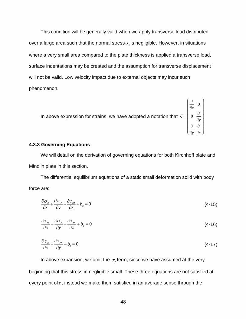
In above expression for strains, we have adopted a notation that
0
0
x
y
y x
4.3.3 Governing Equations
We will detail on the derivation of governing equations for both Kirchhoff plate and
Mindlin plate in this section.
The differential equilibrium equations of a static small deformation solid with body
force are:
0xyx xz
xbx y z
(4-15)
0xy y yz
ybx y z
(4-16)
0yzxz
zbx y
(4-17)
In above expansion, we omit the z term, since we have assumed at the very
beginning that this stress in negligible small. These three equations are not satisfied at
every point of z , instead we make them satisfied in an average sense through the

49
thickness of the plate. This is accomplished by requiring the equations and their
moments be satisfied on both side of the equation on an average sense. The notation
used is shown in Figure 4-3.
Integrating the Equation 4-15 in the thickness h direction, we have
2 2 2 2
2 2
2 2 2 2
( ) 0
h h h h
x xzx x xy xz h xz h x
h h h h
xyb dz dz dz b dz
x z x yy
0xyx
x
PPq
x y
(4-18)
Where2
2 2
2
h
x xz h xz h x
h
q b dz
,2
2
h
x x
h
P dz
, 2
2
h
xy xy
h
P dz
.
Multiply Equation 4-15 with z and integrate in the thickness h direction, we get
2 2 2 2 2
2 2
2 2 2 2 2
( ) 0
h h h h h
x xzx x xy xz xz h xz h x
h h h h h
xyz b dz z dz z dz dz z z zb dz
x z x yy
0xyx
xz x
MMS m
x y
(4-19)
Where2
2
h
x x
h
M z dz
, 2
2
h
xy xy
h
M z dz
and2
2 2
2
h
x xz h xz h x
h
m z z zb dz
.
Integrating the Equation 4-16 in the thickness h direction, we obtain
2 2 2 2
2 2
2 2 2 2
( ) 0
h h h h
xy y yz h yz h y
h h h h
xy y yz
y dz dz dz b dzx y
bx y z
0xy y
y
P Pq
x y
(4-20)

50
Where2
2 2
2
h
y yz h yz h y
h
q b dz
, 2
2
h
xy xy
h
P dz
,2
2
h
y y
h
P dz
Multiply Equation 4-16 with z and integrate in the thickness h direction, we get
2 2 2 2 2
2 2
2 2 2 2 2
( ) 0
h h h h h
xy y yz yz h yz h y
h h h h h
xy y yz
yz dz z dz z dz dz z z zb dzx y
bx y z
0xy y
yz y
M MS m
x y
(4-21)
Where 2
2
h
y y
h
M z dz
2
2
h
xy xy
h
M z dz
and 2
2 2
2
h
y yz h yz h y
h
m z z zb dz
Integrating the Equation 4-17 in the thickness h direction, we obtain
2 2 2 2
2 2 2 2
( ) 0
h h h h
xz yz z
h h h h
yzxzz dz dz dz b dz
x yb
x y
0yzxz
z
SSq
x y
(4-22)
Where2
2
h
z z
h
q b dz
, 2
2
h
xz xz
h
S dz
,2
2
h
yz yz
h
S dz
Multiply Equation 4-17 with z and integrate in the thickness h direction, we get
2 2 2 2
2 2 2 2
( ) 0
h h h h
xz yz z
h h h h
yzxzzz dz z dz z dz zb dz
x yb
x y
0yzxz
z
MMm
x y
(4-23)

51
Where2
2
h
xz xz
h
M z dz
, 2
2
h
yz yz
h
M z dz
and 2
2
h
z z
h
m zb dz
Omitting the in plane terms in Equations 4-18 to 4-23, we finally have the
governing equations as
0xyx
xz x
MMS m
x y
(4-24)
0xy yyz y
M MS m
x y
(4-25)
0yzxz
z
SSq
x y
(4-26)
4.3.4 Constitutive Relationship
In this section, we will derive the relationship between the plate resultants and the
displacement and rotations.
As in last section, the shell resultants have been defined as
x x
y xh
xy xy
M
M z dz
M
, xz xz
hyz yz
Sdz
S
Using the stress-strain relationship and the strain-displacement relation, we can
write the resultants in term of displacement and rotations as
2 2
2 2
h hx x x
y y y
h h
xy xy xy
M
M z dz z dz
M
M C D (4-27)
Where 2
1 0
1 0(1 )
0 0 (1 ) / 2
vE
vv
v
C , 3
12
hD C .

52
2 2 2
2 2 2
h h h
xz xz
yz yzh h h
xz
yz
dz dz kG w dz wS
S
S (4-28)
where kGh . Constant k is added here to account for the fact that shear stresses
aren’t constant across the section. A value of 5 / 6k is the exact for rectangular,
homogeneous section and corresponds to a parabolic shear stress distribution. Details
about how to derive this constant can be found in Appendix C.
In next section, the analytical solution using above governing equation for various
Kirchhoff plate and Mindlin plate is presented. The purpose of this work is to compare
the analytical result with numerical result using developed Mindlin plate elements.
Hence, evaluate the performance of those elements.
4.4 Analytical and Exact Solution
Before proceeding to mixed formulation of Mindlin plate problem, the analytical or
exact solutions for those benchmark problems are derived for the purpose of comparing
results and hence testing the validity of our numerical solution. Since this thesis is
mainly focus on the finite element analysis of various kinds of Mindlin plates, we provide
the analytical or exact solution without any further derivation. For more details, one can
refer to standard textbooks on plates and shells, such as Timoshenko et al. [18] and
Reddy et al. [19].
The benchmark problems will be studied here are: cantilever plate, clamped and
simply-supported square plate, clamped and simply-supported circular plate and
clamped and simply-supported 30 degree and 60 degree skew plates.
For simplicity, we utilize following non-dimensional constants for all testing
examples.

53
Young’s modulus E = 1.12e10; Poisson’s ratio v = 0.3;
Uniform load p = 100 or bending moment m = 100;
Notations for geometries are as following:
Lx: Length of edge x; a: Edge length; r: radius; t: thickness.
The thickness varies among 0.1 and 1, so as to test the validation of the element
for different length/thickness ratio.
4.4.1 Cantilever Plate
Cantilever plate is studied here for the purpose of testing the performance of new
elements when only shear force or bending moment is applied. The cantilever in Figure
4-4 is clamped at the left edge and constant shear force or bending moment, both with
value of 100, is applied separately at the free end.
Due to the loading condition and the length to width ratio, Cantilever plate can be
viewed as 1-D plate undertaking cylindrical bending. In these cases, when shear force
or bending moment applied separately, the transversal deflection is derived here using
1-D assumption. And the results from using Timoshenko beam theory are also provided
here without derivation. For more details, one can refer to Timoshenko et al. [18].
Shear force applied
Using plate theory:
The deflection of the cantilever is
32 1
1
11
ˆ ˆ( ) ( )
2 3
x xS S Lxw x L x
D (4-29)
where 11D is the component of stiffness matrix D in row one and column one.
Using beam theory:
The deflection of the beam using beam theory is

54
32
1
ˆ( ) ( )
2 3
xS xw x L x
EI (4-30)
where E is the Young’s modulus, and I is the moment of inertia, 3
2
12
L hI .
Bending moment applied
A positive bending moment of 100 is applied at the free end.
Using plate theory:
The deflection of the cantilever is
2
11
ˆ( )
2
xMw x x
D
(4-31)
Using beam theory:
From Timoshenko beam theory, we can have the deflection of the beam is
2ˆ
( )2
xMw x x
EI (4-32)
4.4.2 Square Plate
Square plate is conventionally used to assess the element performance. Both
camped and simply-supported cases are studied here. The plate is subjected to a
uniformly distributed load with value of 100. The dimension is shown in Figure 4-5.
Clamped
The general analytical solution for problem of this case is not easy to be obtained
using any series solution. But the exact solution of deflection and bending moments at
the center can be found in numerous in literatures. Below, same valuable results are
given both for thin and thick case. For details, one can refer to the references.
The transverse displacement and bending moment solution:
Thin case:

55
Here, we present several solutions, analytical and exact, so as to fully study the
performance of elements using IBFEM.
Analytical solution by Timoshenko et al. [18]:
The central deflection is
40.00126c
r
qaw
D (4-33)
The central bending moments are
20.0231x yM M qa (4-34)
The exact solution by ZienKiewicz et al. [22]:
The central deflection is
40.00126748c
r
qaw
D (4-35)
The central bending moments are
20.02290469x yM M qa (4-36)
Exact solution by Taylor et al. [17]:
The central deflection is
40.001265319087c
r
qaw
D (4-37)
The central bending moments are
20.02290508352x yM M qa (4-38)
Thick case:
Exact solution by ZienKiewicz et al. [22]:
The central deflection is

56
40.00150442c
r
qaw
D (4-39)
The central bending moments are
20.02319536x yM M qa (4-40)
Simply-supported
The transverse displacement and bending moment solution:
Thin case:
From Timoshenko et al. [18], the deflection of Kirchhoff plate of this case is
2 24 21 1
2
( , ) sin sin
( )
ijK
i j
r
q i x j yw x y
i j a aD
a
(4-41)
where
2
0 0
4( , )sin sin
a a
ij
i x j yq q x y dxdy
a a a
, and flexural rigidity
3
212(1 )r
EhD
v
The bending moments are
2 2
222 2
1 1
2 2
222 2
1 1
222 2 2
1 1
1sin sin ;
1sin sin ;
1cos cos
K
x ij
i j
K
y ij
i j
K
xy ij
i j
i vj i x j yM q
a ai j
vi j i x j yM q
a ai j
ij i x j yM q
a aa i j
(4-42)
An approximate result was also given by Timoshenko et al. [18] as
The central deflection is
40.00406237c
r
qaw
D (4-43)

57
The central bending moments are
20.0479x yM M qa (4-44)
The exact solution by ZienKiewicz et al. [22]:
The central deflection is
40.00410658c
r
qaw
D (4-45)
The central bending moments are
20.04825772x yM M qa (4-46)
Thick case:
According to Reddy et al. [19], the deflection of Mindlin plate of this case is the
sum of the deflection of Kirchhoff plate and the Marcus moments. That’s
( , ) ( , )K
M Kw x y w x y
(4-47)
where
K is the Marcus moment of Kirchhoff plate.
Of this case, the Marcus moment is given by
2
2 221 1
2
( , ) , sin sin
( )
ijK K
r
i j
q j x i yx y D w x y
i j a a
a
(4-48)
Using above deflection relationship between Kirchhoff plate and Mindlin plate of
this case, we have the deflection for Mindlin plate as
2 24 21 1
2
( , ) sin sin
( )
ijM
i j
Q j x i yw x y
i j a a
a
(4-49)

58
where
2 22
2( )
16
ij ij
i jh
aQ q
The bending moments for thick case are
;
;
.
M K
x x
M K
y y
M K
xy xy
M M
M M
M M
(4-50)
The solution also given by ZienKiewicz et al. [22] as
The central deflection is
40.00461856c
r
qaw
D (4-51)
The central bending moments are
20.05096269x yM M qa (4-52)
4.4.3 Circular Plate
A circular plate under uniformly distributed load with clamped and simply
supported boundary conditions is considered here. It’s a good problem to test the
validity of imposing essential boundary condition using Implicit Boundary Method. The
geometry of this circular plate is shown in Figure 4-6.
Clamped
The transverse displacement and bending moment solution:
Thin case:
In Timoshenko et al. [18], the deflection in the form as

59
2 2 2
0( ) ( )64
K
r
qw r r r
D (4-53)
And the bending moment
2 2
0
2 2
0
(1 ) (3 ) ;16
(1 ) (1 3 )16
K
r
K
qM v r v r
qM v r v r
(4-54)
Thick case:
For simply-supported circular plate, according to Reddy et al. [19], the relationship
of deflection and bending moments between Mindlin plate and Kirchhoff plate is
( ) ( ) ;
( ) ( );
( ) ( )
KM K
r
M K
r r
M K
Cw r w r
D
M r M r
M r M r
(4-55)
where
0 0
;1
( ) ( )
(1 )
K KK r
K K
r
M M
v
M r M rC
v
Simply-supported
The transverse displacement and bending moment solution:
Thin case:
From Timoshenko et al. [18], the deflection of a simply-supported plate is of the
form as
2 22 20
0
( ) 5( )
64 1
K q r r vw r r r
D v
(4-56)
The bending moments are

60
2 2
0
2 2
0
( ) (3 )( );16
( ) (3 ) (1 3 )16
K
r
K
qM r v r r
qM r v r v r
(4-57)
Thick case:
The relation between Mindlin plate and Kirchhoff plate is the same as that in the
clamped case:
( ) ( ) ;
( ) ( );
( ) ( )
KM K
r
M K
r r
M K
Cw r w r
D
M r M r
M r M r
(4-58)
where
0
;1
( )
(1 )
K KK r
K
M M
v
M rC
v
4.4.4 30-degree Skew Plate
Skew plate usually being utilized in testing the performance of distorted element.
In order to test the validity of the Implicit Boundary Method for imposing essential
boundary condition, skew plate is a valuable problem for this purpose. We directly
provide some results for skew plate according to Liew [14] and Sengupta [16]. For more
details, one can refer to Liew [14] and Sengupta [16]. The geometry of this plate is
shown in Figure 4-7.
Clamped
The transverse displacement solution:
Thin case:
According to Sengupta [16], the deflection at the center is

61
40.000109125c
r
w qaD
(4-59)
For thick case, there is no analytical solution or exact solution available in
literature.
Simply-supported
The transverse displacement solution:
Thin case:
According to Liew [14] et al., the deflection at the center is
40.0004174375c
r
w qaD
(4-60)
Thick case:
According to Liew et al. [14], the deflection at the center is
40.0005176875c
r
w qaD
(4-61)
4.4.5 60-degree Skew Plate
The geometry of this plate is shown in Figure 4-8.
Clamped
Transverse displacement solution:
Thin case:
According to Sengupta [16], the deflection at the center is
40.0007709375c
r
w qaD
(4-62)
For thick case, there is no analytical solution or exact solution available in
literature.

62
Simply-supported
The transverse displacement solution:
Thin case:
According to Liew et al. [14], the deflection at the center is
40.00261925c
r
w qaD
(4-63)
Thick case:
According to Liew et al. [14], the deflection at the center is
40.0029833125c
r
w qaD
(4-64)
Figure 4-1. Configuration for CPT

63
Figure 4-2. Configuration for FSDT
Figure 4-3. Definitions of variables for plate approximations

64
Figure 4-4. Geometry of cantilever plate
Figure 4-5. Geometry of square plate
Figure 4-6. Geometry of circular plate

65
Figure 4-7. Geometry of 30-degree skew plate
Figure 4-8. Geometry of 60-degree skew plate

66
CHAPTER 5 MIXED FORMULATION FOR MINDLIN PLATE
We will present the derivation of mixed form for Mindlin plate and validate our
IBFEM elements in Chapter 5. Details will focus on deriving the mixed weak form and
imposing essential boundary condition (EBC) using Implicit Boundary Method. The
governing equations for Mindlin plate are already derived in Chapter 4. So we begin the
finite formulation with the matrix form in Chapter 5.
5.1 Mixed Form
Writing in matrix form, the governing equation system is
0
0
Mx S mx y xz xM y S myz yMx y xy
0 (5-1)
T M S m 0 (5-2)
0
Sxz
qzSx y
yz
(5-3)
0T q S (5-4)
Generally, m is not included in the plate theory.
Equations 5-1 to 5-4 constitute the governing equations in the plate theory.
Eliminating the bending moment M , we have the three governing equations as:
0T q S (5-5)
T D S 0 (5-6)
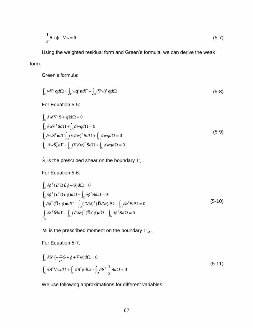
67
1w
S 0 (5-7)
Using the weighted residual form and Green’s formula, we can derive the weak
form.
Green’s formula:
( )T T Tw d w d w d
q q n q (5-8)
For Equation 5-5:
[ ] 0
0
( ) 0
ˆ ( ) 0s
T
T
T T
T T
n
w q d
w d wqd
w d w d wqd
w d w d wqd
S
S
S n S
S S
(5-9)
ˆnS is the prescribed shear on the boundary s .
For Equation 5-6:
( ) 0
( ) 0
( ) ( ) ( ) 0
ˆ ( ) ( ) 0
M
T T
T T T
T T T
T T T
d
d d
d d d
d d d
D S
D S
D n D S
M D S
(5-10)
M is the prescribed moment on the boundary M .
For Equation 5-7:
1( ) 0
10
T
T T T
w d
wd d d
S S
S S S S
(5-11)
We use following approximations for different variables:

68
ˆ ˆˆ , ,
ˆ ˆˆ , ,
w s
w s
w
w
N w N S N S
N w N S N S
(5-12)
Substitute above approximation 5-12, into Equations 5-9 to 5-11, the weak form
system can be represented as
ˆ
ˆ
ˆ
T
wT
b
w0 0 E f
0 K C f
E C H 0S
(5-13)
Where
( ) ( )
1
ˆ
ˆs
M
Tb
Ts w
Ts
Ts s
T Tw w w n
T
d
d
d
d
qd S d
d
K N D N
E N N
C N N
H N N
f N N
f N M
For fairly thin plate, and1T
s sd
H N N 0 , where sN is the shape
function for shearS . As the thin plate limit is approached, there are certain necessary
criteria should be satisfied in order to achieve the solution stability.
According to Zienkiewicz et al. [21], certain necessary but not sufficient count
conditions must be satisfied in order to develop useful and robust elements. The count
conditions are:
w sn n n (5-14)
s wn n (5-15)

69
Where n , sn and
wn are the numbers of , S and w parameters. When this count
conditions are not satisfied then the equation system will be either locked or singular.
Several elements satisfy these criterions are presented in Table 5-1.
In Table 5-1, we can see that the 4-node element ([2]) fails the count condition for
four-element patch test and the 9-node element ([7]) fails the count condition for single
element patch test, but the margin is small. If we increase the element number for the
patch test, this count condition will be satisfied. The 5-node element, depicted in above
table, passes the count condition for both single element and four element patch test,
but it results in singular stiffness matrix, which illustrate the fact that the count condition
is just a necessary, but not sufficient condition to ensure the system solvable and
stable.
In the next section, we will employ discrete collocation method to impose the
above count condition and finally arrive at the mixed weak form.
5.2 Discrete Collocation Constraints Method
To some degree, using three-field mixed formulation to achieve satisfactory
performance is limited. But a different approach uses collocation constraints for the
shear approximation on the element boundaries, thus limiting the number of S
parameters and making the count condition more easily satisfied. We will focus on this
method to derive a useful family of Mindlin elements using IBFEM from now on.
The shear strain xz x
w
x
is uniquely determined given and w at all the
nodes. And hence xz xzS is also uniquely determined there. Using this relationship
and imposing the count conditions, the prescribed values of shear at certain nodes are

70
ˆ ˆˆ[ ]w S Q w Q , where wQ and Q are two constant matrices for each interpolation type.
For simplicity, we directly give this expression here. A detailed derivation is presented in
Appendix E.
We will re-derive the two-field mixed weak form by above discrete shear field
collocation method in this section. Instead of using Galerkin’s weighted residual form,
we adopt the principle of minimum potential energy method to derive the weak form for
the static system.
The potential energy of the system is
st fU V (5-16)
Where
2
1 1
2 2
1
2
1 1
2 2
1 1( ) ( )
2 2
1 1[ ( ) ( )]
2 2
1 1 1( ) ( )
2 2
T T
stV h
kT
k Sh
S
T T
k k S Sh h
T T
S Sh
T T
S Sh
T T
U dV dzd
dzdkG
dzd kG dzd
z z dzd d
z dzd d
d
ε Qε ε Qε
εC 0ε γ
γ0
ε Cε γ γ
C γ γ
C γ γ
D S Sd
(5-17)
ˆ ˆs
M
T T
f nV d wqd w d d
u q S M (5-18)
In order to make the potential energy minimum and hence a stable status of the
system, we let
71
1 ˆ ˆ( ) ( ) 0s
M
st f
T T T T T
n
U V
d d w qd w d d
D S S S M (5-19)
Plugging the relation for the shear term, ˆ ˆˆ[ ( )]s w S N Q w Q , into equation 5-19
and interpolate , w .using their shape function, 5-12, respectively, the variation of
potential energy becomes
ˆ ˆ ˆ ˆˆ ˆ( ) ( ) ( ( )) ( )T T T
st s w s wU d d
N D N N Q w Q N Q w Q (5-20)
ˆ ˆ ˆˆ ˆ( ) ( ) ( )
ˆ ˆˆ( )
T T T T T
st w s s w
T T T
s s w
U d d
d
N D N w Q N N Q w Q
Q N N Q w Q
(5-21)
ˆ ˆ ˆ ˆˆ[ ( ) ( ) ( ) ]
ˆ ˆˆ ˆ[ ( ) ] 0
M
s
T T T T T
s s w
T T T T T
w s s w w w n
d d d
d qd d
N D N Q N N Q w Q N M
w Q N N Q w Q N N S
(5-22)
In the above deduction, we only introduced the variation of total strain energy
terms in the first two expressions, 5-20 and 5-21, since for the external force term, there
are no shear collocation terms, and naturally, it follows a traditional routine.
For any arbitrary ˆand ˆw , above Equation 5-22, must satisfied. Hence we obtain
the weak form as
ˆ ˆˆ( )s
T T T T
w s s w w w nd qd d
Q N N Q w Q N N S (5-23)
ˆ ˆ ˆˆ( ) ( ) ( )
M
T T T T
s s wd d d
N D N Q N N Q w Q N M (5-24)
Rearranging terms in Equations 5-23 and 5-24 and being sorted in matrix form, we
have the weak form for two-field mixed formulation as
T d
X fB DB (5-25)

72
Where
, , ,ˆ
ˆs w s
w
D 0B D X f
0
0 N
N N
w f
fQ Q.
So far, we have finished the derivation of two-field mixed formulation using
discrete shear field collocation method. Some post-processing issues are also
discussed in following content.
Strains and Stresses
After solving the equation system for wand at each node, the associated strains
and stresses are of our interest sometimes. Hence, it’s important to give a hint on how
to obtain these quantities for the implementation.
ˆ[ ]
ˆ ( )
x
y
xy
s w s s
xz
yz
w0 NB X
N Q N Q N w
(5-26)
We can calculate the in plane strains at any layer on the condition that Equation 5-
26 is calculated ahead. The in plane strains on the top surface of the plate are
2
x x
t y y
xy xy
h
ε (5-27)
For bottom in plane strains, due to the linearity with respect to thickness h , it has
the same magnitude as those of the top surface of the plate, but in the opposite
direction.
After computing the in plane strains, the corresponding stresses on the top surface
of the plate also can be calculated by constitutive relationship as

73
x
t y t
xy
σ Cε (5-28)
where C is the isotropic elasticity matrix.
The average transverse shear stresses can be computed as
xz xz
yz yz
(5-29)
Equation 5-29 for the transverse shear stresses is just in an average sense. Most
of times, it is of little use to predict the stress loading condition. In order to get a more
accurate transverse stresses distribution along the thickness, the equilibrium equations
of the static system is used for this purpose, just as what we did to derive the shear
correction factor in Appendix C. For more details, one can refer to Appendix C.
Those bending moments and shear forces also can be calculated by
ˆ
[ ][ ]ˆ ( )
x
y
xy
s w s sx
y
M
M
M
S
S
w0 N DD 0D B X
N Q N Q N w0
(5-30)
Again, the shear forces are also in an average sense. One can calculate the exact
shear force distribution once given the transverse stresses distribution.
5.3 Applying EBC Using Implicit Boundary Method
Two important issues in developing IBFEM for mixed formulations is how to
constructing the step function and solution structure and imposing the essential
boundary condition. Various ways of constructing these functions are already presented
in the Chapter 1. One can refer to those references for details. In this section, we will
focus on the Implicit Boundary Method utilized by Kumar et al. [11]-[13].

74
Solution structure and step function
The solution structure to ensure the imposed essential boundary condition for the
transverse displacement and rotations are
ˆ ˆ ˆ( ) ( ) , ( ) ( )
ˆ ˆ ˆ( ) ( ) , ( ) ( )
w g a w g
g a g
w H w w w H w
x x x x
x H x x H x (5-31)
where H is the step functions to be constructed, ˆˆ ,a aw are the prescribed essential
boundary condition, and ˆˆ ,g gw are the nodal values.
H can be constructed as
0 0
(2 ), 0
1
iH
(5-32)
where is the distance between points to the boundary lines in the bi-normal
direction, and is the transition width in order to avoid computation problem of sharp
change from 0 to1. For transverse displacement, 1i , for rotations, 1,2i .
Total strain energy
In order to impose EBC, the two-field mixed form needs to be modified. We use
the principle of potential energy method to re-derive the weak form using IBFEM.
The potential energy of the system is
1 1 1 ˆ ˆ( ) ( )2 2 s
M
T T T T T
nd d w qd w d d
D S S S M (5-33)
In order to make the potential energy minimum hence make the system stable, we
let the variation of the potential energy to be zero. That is

75
1 ˆ ˆ( ) ( )
ˆ ˆ( ) ( ) 0
s
M
s
M
T T T T T
n
T T T T T
s s n
d d w qd w d d
d d w qd w d d
D S S S M
D γ γ S M
(5-34)
Rewriting above equation in a matrix form, the equation becomes
0 ˆ ˆ( ) 0
0 s
M
T T T T T
s n
s
d w qd w d d
Dγ S M
γ
(5-35)
For convenience of elaboration, we define
s
εγ
(5-36)
0
0
DD (5-37)
Hence the total strain energy term of Equation 5-35 can be rewritten as
0
( )0
T T
st s
s
Td dU
Dγ
γε Dε
(5-38)
Knowing that s w γ , and plugging in the trial solution and test function,
Equation 5-31, the integrant of 5-38 can be expressed as
) ( ))
( )( )
T
g w g g
g aT Tg g a
a aw g g
H wwH w
H HH
ε Dε D ε D ε εH
(5-39)
Where
),
( )
g ag a
a aw g g wH w
Hε ε
H
(5-40)

76
aε results from the prescribed essential boundary conditions. For implementation
purpose, we can move this term to the RHS, considered to be a force term together with
the original external force terms. This fictitious force term is
a
Tg ad
F ε Dε (5-41)
aε can be rewrite as
ˆ
ˆ a
aaa a
a a w a
w
w
0 Nε B X
N N
(5-42)
The LHS can be further simplified as follows:
Separating gε into two parts as,
gg
gg g w gw H w
Hε
(5-43)
Also, we define here
1
g
gg gw
ε
(5-44)
2
g
gw gH w
Hε
(5-45)
Above two terms also can be expressed in terms of nodal displacement as:
1 1
ˆ
ˆ a
gg
g gg gg g w g
w
w
0 Nε B X B X
N N
(5-46)
2 2
ˆ
ˆ
gg
gg gw g w w g
w
H w H
H 0 H Nε B X
N 0
(5-47)
Expanding g g
Tε Dε , we can have
77
1 2 1 2 1 1 1 2 2 1 2 2( ) ( )g g
T T T T T Tg g g g g g g g g g g g ε Dε ε ε D ε ε ε Dε ε Dε ε Dε ε Dε (5-48)
Apparently, 1 1Tg gε Dε is what we have used in the collocation method for inner
elements. For boundary elements, there are two more additional terms, that 2gε and
aε ,
due to the essential boundary condition.
Integration issue
For terms not including the step functionwH and H , we use volume integration.
That
1
1 1 1
12
e T
g g g
A
hd dA
K B DB (5-49)
1
12
e T
q w
A
hq d dA
F N (5-50)
1
1
ˆ2
e T
s w
A
hd dA
F N S (5-51)
1
1
ˆ2
e T
m
A
hd dA
F N M (5-52)
For terms contain these two step functions, instead of using volume integration,
we can use boundary integration, since the step functions are define as constant except
the boundary transit region.
1
0
1
1 02
e
e
e T T
g g g g g
hd d d d
K B DB B DB (5-53)
1
0
1
1 02
e
e
T
a g a
hd d d
F B DB (5-54)

78
So far, we have successfully imposed the EBC using Implicit Boundary Method.
And details about formulation and implementation are given. In next section, we will
compare our numerical solution with analytical or exact solution provided in Chapter 4.
5.4 Numerical Results
Numerical results for the benchmark problems in section 4.3 will be studied in this
section. S4R and S8R5 elements in commercial package ABAQUS were also used in
this analysis to test the performance of the developed elements. Comparison among
numerical results, exact solutions and analytical solutions are presented. Within each
example, the convergence of total strain energy is also studied.
5.4.1 Cantilever Plate
A cantilever plate with background mesh is shown in Figure 5-1.
Shear applied
Shear is applied at the free end of the cantilever plate. The relevant result of this
case is provided in Table 5-2. And the distribution of the transverse displacement after
deformation of thin case is presented in Figure 5-2. The convergence plots of the total
strain energy for both thin and thick cases are provided in Figure 5-3 and Figure 5-4
respectively.
Bending moment applied
Only bending is applied at the free end in this case. The relevant result of this case
is presented in Table 5-3, both thin and thick cases. The distribution of the transverse
displacement after deformation for thin case is presented in Figure 5-5. And the total
strain energy plots are in Figure 5-6 and Figure 5-7.

79
5.4.2 Square Plate
We utilize two kinds of background mesh for the interpolation for this very
conventional benchmark problem, as shown in Figure 5-8 and Figure 5-9. The results
obtained from both these two approximations using IBFEM converges to the exact
solution from Zienkiewicz et al. [22]. Data tabulated in Table 5-4 to Table 5-7 are
collected using background pattern one (Figure 5-8).
Fully clamped
The relevant data of this case is given in Table 5-4 and Table 5-5. The deformed
transverse displacements for both two mesh patterns are provided in Figure 5-10 and
Figure 5-11 respectively. And the convergence plots for the total strain energy are in
Figure 5-12 and Figure 5-13.
Simply-supported
The relevant data of this case is given in Table 5-6 and Table 5-7. The
convergence plots for the total strain energy is in Figure 5-14 and Figure 5-15.
5.4.3 Circular Plate
A typical background mesh for this circular plate is depicted in Figure 5-16. Table
5-8 to Table 5-11 give the relevant testing results.
Fully clamped
The relevant data of this case is given in Table 5-8 and Table 5-9. And the
convergence plot for the total strain energy is in Figure 5-18 and Figure 5-19. A graph
for the transverse displacement of the thick case is given in Figure 5-17.
Periphery is simply-supported
The relevant data of this case is given in Table 5-10 and Table 5-11. And the
convergence plot for the total strain energy is in Figure 5-20 and Figure 5-21.

80
5.4.4 30-degree Skew Plate
A typical background mesh for this 30-degree skew plate is provided in Figure 5-
22. Table 5-12 to Table 5-15 give the relevant testing results.
Fully clamped
We found that the analytical or exact solution for a comparatively thick plate, such
as length/thickness ratio is 0.1, is very rare, even impossible to refer to in literature. Due
to this limitation, we will not provide any analytical solution or exact solution for this case
for comparison. We only compare our results with S4R and S8R5 elements. The
relevant data are given in Table 5-12 and Table 5-13. The deformed transverse
displacement distribution is presented in Figure 5-23, and the convergence plot for the
total strain energy is in Figure 5-25 and Figure 5-26.
Fully simply-supported
Since there is bending moment singularity at the obtuse corners for simply
supported thin plate, we choose not to provide the bending moment for this case here,
only with one figure, Figure 5-24, to demonstrate the singularity of bending moment at
the obtuse corners. The relevant data of this case are given in Table 5-14 and Table 5-
15. And the convergence plot for the total strain energy is in Figure 5-27 and Figure 5-
28.
5.4.5 60-degree Skew Plate
A typical background mesh using 10X10 Q16 element is shown in Figure 5-29.
Fully clamped
The analytical or exact solution for a comparatively thick skew plate is also very
rare, even impossible to find in literature. For this case, we only compare the result with
S4R and S8R5 elements. The relevant data of this case are formatted in Table 5-16 and

81
Table 5-17. And the convergence plot for the total strain energy is in Figure 5-32 and
Figure 5-33. The deformed transverse displacement distribution is in Figure 5-30.
Fully simply-supported
The bending moment singularity also occurs in this case at small thickness. This
singularity is demonstrated in Figure 5-31. The relevant data of this case are given in
Table 5-18 and Table 5-19. And the convergence plot for the total strain energy is in
Figure 5-34 and Figure 5-35.
5.4.6 Flange Plate
In addition to the above conventional problems, we also present the analysis result
using IBFEM for an arbitrary shaped plate. It also aims to test the performance of these
elements for arbitrary shapes. The plate is clamped at all four corner holes. The
geometry of this plate is provided in Figure 5-36, and a typical background mesh is
presented in Figure 5-37. The result data tabulated in Table 5-20 is for the four inner
holes clamped scenario. The convergence plot for the total strain energy and transverse
displacement plot are in Figure 5-39, Figure 5-40 and Figure 5-38 respectively.
5.5 Concluding Remarks
Implicit Boundary Finite Element method was employed in Chapter 5 to develop a
family of Mindlin plate elements. Discrete shear field collocation method is used to make
the count condition satisfied. Implicit Boundary Method is adopted to impose the
essential boundary condition. Several benchmark problems and one arbitrary shape
problem are tested in order to fully assess the performance of these elements. From the
obtained results and comparison with the exact solution, analytical solution and that
from S4R and S8R5 of commercial package, these developed elements are valid and
robust. In conclusion, employing the Implicit Boundary Finite Element Method can solve

82
plate problem for both thin and thick cases using a background mesh and equations of
the boundary to avoid generating a conforming mesh.
Table 5-1. Location of three interpolation variables and the associated count conditions
for patch test
Element
Clamped edges Relaxed edges
One - element patch Four - element patch One - element patch Four - element patch
s
w
n
n
w
s
n n
n
s
w
n
n
w
s
n n
n
s
w
n
n
w
s
n n
n
s
w
n
n
w
s
n n
n
0
0
0
0
4
1
3
4 (F)
4
3
9
4
12
8
24
12
2
1
3
2
12
5
15
12
6
4
12
6
20
12
36
20
0
0
0
0
8
5
15
8
8
7
21
8
24
20
60
24
4
1
3
4 (F)
24
9
27
24
12
8
24
12
40
24
72
40
12
4
12
12
60
25
75
60
24
15
45
24
84
48
144
84
: deflection w interpolation node; : rotations ,x y interpolation node; : Shear xS
collocation point; : Shear yS collocation point.

83
Table 5-2. Cantilever plate (Shear force applied at free end)
Mesh density
a/t = 10 tip displacement w
( 0510 )
a/t = 100 tip displacement w
( 0210 )
Q4 Q8 Q9 Q16 S4R S8R5 Q4 Q8 Q9 Q16 S4R S8R5
10X1 3.558 3.604 3.583 3.583 3.581 3.583 3.530 3.575 3.536 3.539 3.554 3.538 20X2 3.575 3.588 3.584 3.584 3.585 3.586 3.530 3.552 3.539 3.539 3.542 3.537 50X5 3.582 3.585 3.585 3.585 3.584 3.587 3.536 3.542 3.539 3.539 3.539 3.538
100X10 3.584 3.585 3.586 3.585 3.585 3.588 3.538 3.540 3.539 3.539 3.539 3.539
Analytical 3.571 3.571
Table 5-3. Cantilever plate (Bending moment applied at free end)
Mesh density
a/t = 10 tip displacement w
( 0610 )
a/t = 100 tip displacement w
( 0310 )
Q4 Q8 Q9 Q16 S4R S8R5 Q4 Q8 Q9 Q16 S4R S8R5
10X1 5.324 5.342 5.339 5.342 5.348 5.342 5.324 5.342 5.321 5.326 5.348 5.325 20X2 5.337 5.342 5.342 5.343 5.347 5.345 5.320 5.334 5.325 5.325 5.332 5.323 50X5 5.341 5.343 5.343 5.344 5.344 5.344 5.323 5.327 5.326 5.326 5.326 5.325
100X10 5.343 5.344 5.344 5.344 5.344 5.344 5.325 5.326 5.326 5.326 5.326 5.326
Analytical 5.357 5.357
Table 5-4. Uniformly loaded, clamped square plate [a/t = 10]
Mesh density
Central displacement w
( 0610 )
Central bending moment x yM M
( 0210 )
Q4 Q8 Q9 Q16 S4R S8R5 Q4 Q8 Q9 Q16 S4R S8R5
10x10 1.457 1.642 1.482 1.467 1.470 1.466 2.335 2.539 2.368 2.298 2.278 2.375 20x20 1.464 1.515 1.470 1.467 1.468 1.467 2.324 2.375 2.332 2.315 2.310 2.333 50x50 1.467 1.475 1.468 1.467 1.467 1.467 2.321 2.329 2.322 2.319 2.318 2.322
100x100 1.467 1.469 1.467 1.467 1.467 1.467 2.320 2.322 2.320 2.320 2.320 2.321 150x150 1.467 1.468 1.467 1.467 1.467 1.467 2.320 2.321 2.320 2.320 2.320 2.320
Exact 1.467 2.320
Table 5-5. Uniformly loaded, clamped square plate [a/t = 100]
Mesh density
Central displacement w
( 0310 )
Central bending moment x yM M
( 0210 )
Q4 Q8 Q9 Q16 S4R S8R5 Q4 Q8 Q9 Q16 S4R S8R5
10x10 1.227 1.417 1.251 1.236 1.239 1.236 2.316 2.516 2.338 2.269 2.253 2.346 20x20 1.234 1.286 1.240 1.236 1.237 1.236 2.297 2.349 2.302 2.286 2.281 2.304 50x50 1.236 1.245 1.237 1.236 1.236 1.236 2.292 2.300 2.293 2.290 2.289 2.293
100x100 1.236 1.238 1.236 1.236 1.236 1.236 2.291 2.293 2.291 2.291 2.291 2.291 150x150 1.236 1.237 1.236 1.236 1.236 1.236 2.291 2.292 2.291 2.291 2.291 2.291
Exact 1.236 2.290

84
Table 5-6. Uniformly loaded, simply-supported square plate [a/t = 10]
Mesh density
Central displacement w
( 0610 )
Central bending moment x yM M
( 0210 )
Q4 Q8 Q9 Q16 S4R S8R5 Q4 Q8 Q9 Q16 S4R S8R5
10x10 4.395 4.602 4.499 4.501 4.472 4.476 5.012 5.204 5.117 5.075 4.968 5.127 20x20 4.465 4.518 4.503 4.501 4.493 4.498 5.066 5.115 5.102 5.091 5.063 5.106 50x50 4.495 4.504 4.502 4.501 4.500 4.501 5.090 5.098 5.097 5.095 5.090 5.098
100x100 4.500 4.502 4.502 4.501 4.501 4.502 5.094 5.096 5.096 5.096 5.094 5.096 150x150 4.501 4.502 4.502 4.501 4.501 4.502 5.095 5.096 5.096 5.096 5.095 5.096
Exact 4.503 5.096
Table 5-7. Uniformly loaded, simply-supported square plate [a/t = 100]
Mesh density
Central displacement w
( 0310 )
Central bending moment x yM M
( 0210 )
Q4 Q8 Q9 Q16 S4R S8R5 Q4 Q8 Q9 Q16 S4R S8R5
10x10 3.954 4.146 3.982 3.978 3.977 3.969 4.793 4.981 4.832 4.781 4.706 4.849 20x20 3.967 4.016 3.982 3.988 3.978 3.975 4.795 4.843 4.813 4.806 4.779 4.813 50x50 3.979 3.987 3.992 3.996 3.988 3.987 4.803 4.811 4.816 4.818 4.808 4.813
100x100 3.988 3.990 3.996 3.997 3.994 3.995 4.811 4.813 4.819 4.819 4.816 4.818 150x150 3.992 3.993 3.997 3.997 3.995 3.996 4.815 4.816 4.819 4.819 4.818 4.819
Exact 4.004 4.826
Table 5-8. Uniformly loaded, clamped circular plate [a/t = 10]
Mesh density
Central displacement w
( 0610 )
Central bending moment rM M
( 0210 )
Q4 Q8 Q9 Q16 S4R S8R5 Q4 Q8 Q9 Q16 S4R S8R5
10x10 0.737 1.194 1.091 1.109 1.110 1.128 1.573 2.199 2.048 1.992 1.970 2.058 20x20 0.970 1.143 1.111 1.113 1.119 1.126 1.860 2.065 2.029 2.012 2.000 2.029 50x50 1.099 1.119 1.112 1.113 1.126 1.129 2.003 2.025 2.020 2.017 2.029 2.035
100x100 1.108 1.115 1.113 1.113 1.126 1.125 2.013 2.020 2.019 2.018 2.030 2.031 150x150 1.111 1.114 1.113 1.113 1.126 1.124 2.016 2.019 2.018 2.018 2.031 2.031
Analytical 1.039 2.031
Table 5-9. Uniformly loaded, clamped circular plate [a/t = 100]
Mesh density
Central displacement w
(0410 )
Central bending moment rM M
Q4 Q8 Q9 Q16 S4R S8R5 Q4 Q8 Q9 Q16 S4R S8R5
10x10 4.745 9.100 9.017 9.313 9.374 9.502 1.348 2.075 2.033 1.985 1.970 2.043 20x20 7.027 9.535 9.371 9.399 9.471 9.504 1.731 2.049 2.026 2.011 2.002 2.028 50x50 8.895 9.459 9.409 9.410 9.535 9.537 1.959 2.025 2.019 2.017 2.029 2.032
100x100 9.253 9.428 9.413 9.413 9.538 9.539 2.000 2.020 2.018 2.018 2.030 2.032 150x150 9.360 9.419 9.413 9.413 9.538 9.539 2.012 2.019 2.018 2.018 2.031 2.031
Analytical 9.522 2.031

85
Table 5-10. Uniformly loaded, simply-supported circular plate [a/t = 10]
Mesh density
Central displacement w
( 0610 ) Central bending moment
rM M
Q4 Q8 Q9 Q16 S4R S8R5 Q4 Q8 Q9 Q16 S4R S8R5
10x10 1.076 3.127 3.046 3.742 3.978 4.053 2.008 4.257 4.180 4.825 5.049 5.182 20x20 1.788 3.535 3.848 3.950 4.029 4.050 2.788 4.536 4.972 5.047 5.114 5.153 50x50 3.497 3.922 3.959 3.982 4.053 4.059 4.591 5.019 5.075 5.096 5.152 5.159
100x100 3.805 3.986 3.989 3.991 4.055 4.055 4.914 5.098 5.106 5.107 5.155 5.157 150x150 3.920 3.986 3.989 4.028 4.056 4.054 5.034 5.102 5.106 5.107 5.156 5.156
Analytical 4.103 5.156
Table 5-11. Uniformly loaded, simply-supported circular plate [a/t = 100]
Mesh density
Central displacement w
( 0310 ) Central bending moment
rM M
Q4 Q8 Q9 Q16 S4R S8R5 Q4 Q8 Q9 Q16 S4R S8R5
10x10 0.737 1.557 1.114 1.532 3.805 3.875 2.002 4.202 4.143 4.795 5.049 5.168 20x20 0.966 1.683 1.706 2.393 3.857 3.875 2.767 4.506 4.962 5.034 5.115 5.153 50x50 1.637 2.215 2.517 3.073 3.881 3.883 4.481 5.013 5.073 5.092 5.152 5.157
100x100 3.120 3.211 3.417 3.743 3.883 3.884 4.912 5.098 5.102 5.107 5.155 5.157 150x150 3.406 3.690 3.708 3.743 3.883 3.884 5.033 5.100 5.106 5.107 5.156 5.156
Analytical 3.900 5.156
Table 5-12. Uniformly loaded, clamped 30-degree skew plate [a/t = 10]
Mesh density
Central displacement w
( 0710 )
Central bending moment xM
( 0110 )
Q4 Q8 Q9 Q16 S4R S8R5 Q4 Q8 Q9 Q16 S4R S8R5
10x10 0.806 2.576 1.717 1.726 1.642 1.767 2.545 7.479 5.183 4.635 4.684 5.087 20x20 1.320 2.106 1.729 1.729 1.695 1.735 3.711 5.767 4.999 4.802 4.626 4.928 50x50 1.662 1.812 1.728 1.728 1.724 1.730 4.624 5.003 4.894 4.859 4.861 4.868
100x100 1.723 1.755 1.728 1.728 1.727 1.728 4.847 4.895 4.877 4.868 4.861 4.880 150x150 1.726 1.742 1.728 1.728 1.728 1.726 4.859 4.878 4.873 4.869 4.868 4.885
Table 5-13. Uniformly loaded, clamped 30-degree skew plate [a/t = 100]
Mesh density
Central displacement w
( 0410 )
Central bending moment xM
( 0110 )
Q4 Q8 Q9 Q16 S4R S8R5 Q4 Q8 Q9 Q16 S4R S8R5
10x10 0.143 1.480 0.971 1.055 0.957 1.062 1.107 6.430 4.685 4.578 4.801 4.880 20x20 0.664 1.362 1.060 1.062 1.027 1.059 3.628 5.731 4.903 4.708 4.554 4.782 50x50 0.967 1.126 1.063 1.062 1.058 1.062 4.490 4.945 4.802 4.764 4.755 4.780
100x100 1.047 1.079 1.062 1.062 1.062 1.062 4.743 4.818 4.782 4.772 4.763 4.776 150x150 1.057 1.070 1.062 1.062 1.062 1.062 4.760 4.794 4.778 4.773 4.772 4.776
Exact 1.064 -

86
Table 5-14. Uniformly loaded, simply-supported 30-degree skew plate [a/t = 10]
Mesh density
Central displacement w
( 0710 )
Central bending moment xM
( 0210 )
Q4 Q8 Q9 Q16 S4R S8R5 Q4 Q8 Q9 Q16 S4R S8R5
10x10 1.217 6.258 4.759 5.004 4.796 5.081 0.366 1.554 1.225 1.217 1.148 1.271 20x20 2.556 5.456 5.001 5.043 4.945 5.050 0.651 1.337 1.267 1.235 1.225 1.269 50x50 4.429 5.140 5.043 5.047 5.031 5.053 1.075 1.277 1.265 1.258 1.259 1.263
100x100 5.001 5.080 5.046 5.047 5.044 5.053 1.247 1.267 1.263 1.262 1.261 1.265 150x150 5.024 5.066 5.047 5.047 5.046 5.049 1.255 1.265 1.263 1.262 1.262 1.264
Exact 5.047 -
Table 5-15. Uniformly loaded, simply-supported 30-degree skew plate [a/t = 100]
Mesh density
Central displacement w
( 0410 )
Q4 Q8 Q9 Q16 S4R S8R5
10x10 0.255 4.584 2.707 3.451 3.897 4.069 20x20 0.867 4.036 3.334 3.802 4.013 4.083 50x50 1.671 4.032 3.909 4.081 4.105 4.118
100x100 3.111 3.909 4.080 4.132 4.130 4.135 150x150 3.410 4.122 4.122 4.138 4.135 4.138
Exact 4.070
Table 5-16. Uniformly loaded, clamped 60-degree skew plate [a/t = 10]
Mesh density
Central displacement w
( 0710 )
Central bending moment xM
( 0210 )
Q4 Q8 Q9 Q16 S4R S8R5 Q4 Q8 Q9 Q16 S4R S8R5
10x10 5.358 11.31 9.446 9.355 9.315 1.033 1.257 2.031 1.751 1.581 1.635 1.764 20x20 8.793 9.916 9.339 9.320 9.302 1.034 1.624 1.766 1.692 1.650 1.665 1.727 50x50 9.237 9.413 9.305 9.304 9.299 1.034 1.669 1.688 1.677 1.670 1.673 1.717
100x100 9.288 9.331 9.300 9.300 9.298 1.034 1.674 1.677 1.675 1.674 1.674 1.715 150x150 9.294 9.315 9.299 9.299 9.298 1.034 1.674 1.675 1.674 1.674 1.674 1.720
Table 5-17. Uniformly loaded, clamped 60-degree skew plate [a/t = 100]
Mesh density
Central displacement w
( 0410 )
Central bending moment xM
( 0210 )
Q4 Q8 Q9 Q16 S4R S8R5 Q4 Q8 Q9 Q16 S4R S8R5
10x10 2.764 8.688 7.539 7.525 7.539 7.527 1.283 1.897 1.728 1.989 1.623 1.704 20x20 5.643 8.072 7.546 7.519 7.521 7.528 1.526 1.750 1.672 1.644 1.645 1.666 50x50 6.872 7.622 7.523 7.517 7.518 7.529 1.622 1.670 1.656 1.652 1.652 1.656
100x100 7.357 7.545 7.519 7.517 7.517 7.529 1.647 1.657 1.654 1.653 1.653 1.654 150x150 7.456 7.530 7.518 7.517 7.517 7.529 1.651 1.655 1.653 1.653 1.653 1.654
Analytical 7.517 -

87
Table 5-18. Uniformly loaded, simply-supported 60-degree skew plate [a/t = 10]
Mesh density
Central displacement w
( 0610 )
Central bending moment xM
( 0210 )
Q4 Q8 Q9 Q16 S4R S8R5 Q4 Q8 Q9 Q16 S4R S8R5
10x10 0.809 3.103 2.898 2.923 2.881 2.999 1.721 4.082 3.895 3.798 3.743 3.937 20x20 2.349 2.975 2.912 2.914 2.900 3.009 3.201 3.932 3.875 3.845 3.829 3.907 50x50 2.837 2.925 2.910 2.910 2.907 3.010 3.768 3.875 3.863 3.858 3.855 3.896
100x100 2.904 2.916 2.909 2.909 2.908 3.010 3.854 3.867 3.861 3.860 3.859 3.895 150x150 2.907 2.914 2.909 2.909 2.909 3.010 3.858 3.865 3.860 3.860 3.860 3.894
Exact 2.909 -
Table 5-19. Uniformly loaded, simply-supported 60-degree skew plate [a/t = 100]
Mesh density
Central displacement w
( 0310 )
Q4 Q8 Q9 Q16 S4R S8R5
10x10 0.352 2.722 2.399 2.489 2.507 2.510 20x20 0.868 2.596 2.487 2.520 2.511 2.517 50x50 1.951 2.551 2.527 2.535 2.524 2.530
100x100 2.430 2.537 2.535 2.537 2.532 2.536 150x150 2.483 2.539 2.536 2.537 2.534 2.537
Exact 2.554
Table 5-20. Uniformly loaded, arbitrary shape plate
Mesh density
a/t = 10 Central displacement w
( 0710 )
a/t = 100 Central displacement w
( 0410 )
Q4 Q8 Q9 Q16 S4R S8R5 Q4 Q8 Q9 Q16 S4R S8R5
20x20 5.606 7.350 6.927 7.310 7.540 7.379 3.235 4.539 4.234 4.551 4.770 4.698 50x50 5.754 7.440 7.275 7.458 7.423 7.356 3.635 4.668 4.610 4.604 4.739 4.698
100x100 7.260 7.502 7.423 7.475 7.368 7.356 4.542 4.749 4.671 4.701 4.707 4.697 150x150 7.070 7.467 7.430 7.475 7.356 7.346 4.505 4.754 4.738 4.704 4.699 4.697
Figure 5-1. A typical background mesh using 20x2 Q4 element
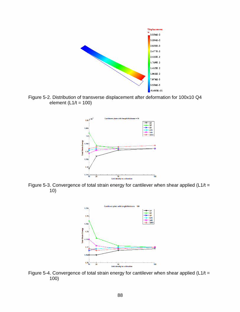
88
Figure 5-2. Distribution of transverse displacement after deformation for 100x10 Q4
element (L1/t = 100)
Figure 5-3. Convergence of total strain energy for cantilever when shear applied (L1/t =
10)
Figure 5-4. Convergence of total strain energy for cantilever when shear applied (L1/t =
100)

89
Figure 5-5. Distribution of transverse displacement after deformation for 100x10 Q4
element (L1/t = 100)
Figure 5-6. Convergence of total strain energy for cantilever when bending moment
applied (L1/t = 10)
Figure 5-7. Convergence of total strain energy for cantilever when bending moment
applied (L1/t = 100)

90
Figure 5-8. A typical background mesh using 10x10 Q9 element
Figure 5-9. A typical background mesh using 10x10 Q9 element
Figure 5-10. Distribution of transverse displacement after deformation for 150x150 Q9
element (t = 0.1)

91
Figure 5-11. Distribution of transverse displacement after deformation for 225x225 Q9
element (t = 0.1)
Figure 5-12. Convergence of total strain energy for clamped square plate (a/t = 10)
Figure 5-13. Convergence of total strain energy for clamped square plate (a/t = 100)

92
Figure 5-14. Convergence of total strain energy for simply-supported square plate (a/t =
10)
Figure 5-15. Convergence of total strain energy for simply-supported square plate (a/t =
100)
Figure 5-16. A typical background mesh using 10x10 Q4 element

93
Figure 5-17. Distribution of transverse displacement after deformation for 150x150 Q4
element (t = 1)
Figure 5-18. Convergence of total strain energy for clamped circular plate (a/t = 10)
Figure 5-19. Convergence of total strain energy for clamped circular plate (a/t = 100)

94
Figure 5-20. Convergence of total strain energy for simply-supported circular plate (a/t =
10)
Figure 5-21. Convergence of total strain energy for simply-supported circular plate (a/t =
100)
Figure 5-22. A typical background mesh using 10x10 Q8 element

95
Figure 5-23. Distribution of transverse displacement after deformation for 200x200 Q8
element (t = 0.1)
Figure 5-24. Distribution of bending moment using 200x200 Q4 element (t = 0.1)
Figure 5-25. Convergence of total strain energy for clamped 30-degree skew plate (a/t =
10)

96
Figure 5-26. Convergence of total strain energy for clamped 30-degree skew plate (a/t =
100)
Figure 5-27. Convergence of total strain energy for simply-supported 30-degree skew
plate (a/t = 10)
Figure 5-28. Convergence of total strain energy for simply-supported 30-degree skew
plate (a/t = 100)

97
Figure 5-29. A typical background mesh using 10x10 Q16 element
Figure 5-30. Distribution of transverse displacement after deformation for 200x200 Q9
element (t = 1)
Figure 5-31. Distribution of bending moment using 200x200 Q4 element (t = 0.1)

98
Figure 5-32. Convergence of total strain energy for clamped 60-degree skew plate (a/t =
10)
Figure 5-33. Convergence of total strain energy for clamped 60-degree skew plate (a/t =
100)
Figure 5-34. Convergence of total strain energy for simply-supported 60-degree skew
plate (a/t = 10)

99
Figure 5-35. Convergence of total strain energy for simply-supported 60-degree skew
plate (a/t = 100)
Figure 5-36. Geometry of flange plate
Figure 5-37. A typical background mesh using 20x20 Q9 element

100
Figure 5-38. Distribution of transverse displacement after deformation for 150x150 Q9
element (t = 0.1)
Figure 5-39. Convergence of total strain energy for arbitrary shape plate (a/t = 10)
Figure 5-40. Convergence of total strain energy for arbitrary shape plate (a/t = 100)

101
CHPATER 6 MIXED FORMULATION FOR 2D MINDLIN SHELL
In plate elements, we are mainly concerned about bending and transverse loading.
Plates subjected to both transverse loading and in-plane stretching is a special case of
shells. Chapter 6 is intended to model this special case, and hence prepare for future
work on curved 3D shell-like structures.
6.1 Governing Equations
The derivation of the governing equations for Mindlin plate has already been done
in Chapter 4. In Chapter 4, we assume that there is no in-plane stretching, therefore,
terms associated with stretching are omitted. In Chapter 6, we will consider in-plane
stretching also. The derivation is the same as in Chapter 4, except that two more
equations are added into the governing equations.
The governing equations are
0xyx
x
PPq
x y
(6-1)
0xy y
y
P Pq
x y
(6-2)
0yzxz
z
SSq
x y
(6-3)
0xyx
xz
MMS
x y
(6-4)
0xy yyz
M MS
x y
(6-5)
Writing in matrix form, the governing equation system can be expressed as

102
0
0
xx
yy
xy
qP
qP
Px y
y x
0 (6-6)
T P q 0 (6-7)
0
0
xxz
yyz
xy
MSx y
MS
My x
0 (6-8)
T M S 0 (6-9)
0xz
zyz
Sq
Sx y
(6-10)
0T q S (6-11)
For clarity, notations used in above equations are rewritten here.
2 2
2 2
h hx x x
y y y
h h
xy xy xy
P
P dz dz
P
P C A u (6-12)
2 2
2 2
h hx x x
y y y
h h
xy xy xy
M
M z dz z dz
M
M C D (6-13)
2 2 2
2 2 2
h h h
xz xz
yz yzh h h
xz
yz
dz dz kG w dz wS
S
S (6-14)
2
1 0
1 0(1 )
0 0 (1 ) / 2
vE
vv
v
C
hA C

103
3
12
hD C
kGh
Equations 6-6 to 6-11 constitute the governing equation system for Chapter 6.
Substituting notation 6-12 to 6-14 into Equations 6-6 and 6-11, respectively, we
can eliminate the in plane forces P and moment M and finally obtain the four governing
equations as:
0
10
T
T
T
q
A u q 0
S
D S 0
S
(6-15)
So far, we have obtained the governing equation for plates including in-plane
stretching. In next section, we will formulate the mixed form for this plate.
6.2 Mixed Formulation
We have already derived the governing equations for Mindlin plate including in-
plane stretching. Next, we will focus on the derivation of the mixed form.
As we have mentioned in the last section, except the first governing equation, the
remaining three are the same as those in Chapter 5. And the weak mixed form for these
three equations are still the same since there is no coupling between in-plane stretching
and transverse bending in our formulation. For simplicity, we will only derive the weak
form for the first equation. For the other three, one can refer to Chapter 5 for details.
Using integration by part and Green’s formula, the weak form of 6-6 to 6-11 can be
deduced as

104
[ ( ) ]
[ ( )]
( ) ( ) ( )
ˆ ( ) ( )P
T T
T T T
T T T
T T T
d
d d
d d d
d d d
u A u q 0
u A u u q 0
u A u n u A u u q 0
u P u A u u q 0
(6-16)
P is the prescribed traction on the boundary P .
The final weak system of the combined Mindlin plate is
ˆ( ) ( )
ˆ ˆˆ( ) ( )
ˆ ˆˆ( ) [ ( ) ( ) ( ) ]
P
s
M
T T T
u u u u
T T T T
s w s w s w s w w n
T T T T
s s w s s
d d d
d d qd d
d d d d
N A N N q N P
N Q N Q w N Q N Q N N S
N Q N Q w N D N N Q N Q N M
(6-17)
Writing in matrix form, the mixed weak form can be expressed as
T d
X fB DB (6-18)
Where
, , ,
ˆ
ˆ
ˆ
u
s w s
u
w
A 0 0
B D 0 D 0 X f
0 0
N 0 0
0 0 N
0 N N
u f
w f
Q Q f
(6-19)
Strains and Stresses
After solving the equations for u , wand at each node, we need to calculate the
associated strains and stresses.
0
0
0
[ ]( )
ˆˆˆ
x
y
xy
x
ys
xy
xz
yz
u
s w s
uB X
N w
N 0 00 0 N
0 N N
uw
Q Q (6-20)

105
Once the membrane strain and curvature are obtained, the in plane strains on any
layer can be immediately calculated. At the height equal to 2
h, the membrane strains on
the top surface of the plate is
0
0
02
x x x
t y y y
xy xy xy
h
ε (6-21)
Using constitutive relationship, we can obtain the corresponding stresses on the
top surface of the plate as
x
t y t
xy
σ Cε (6-22)
where C is the stiffness matrix.
The average transverse shear stresses can be computed as
xz xz
yz yz
(6-23)
We also can calculate the in-plane forces, bending moments and shear forces as
[ ][ ]( )
ˆˆˆ
x
y
xy
x
ys
xy
x
y
u
s w s
PP
P
MM
M
SS
A 0 0 A uD B X 0 D 0 D
N w0 0
N 0 00 0 N
0 N N
uw
Q Q (6-24)

106
6.3 Numerical Examples and Results
The way to impose the EBC is almost the same as what have been done in
Chapter 5. We will not redo the procedures for combined Mindlin plates. One can refer
to Chapter 5 for details.
Examples employed in Chapter 6 are the 60 degree skew plate and square plate
that have been used in Chapter 5. The geometry and elastic constants are exactly the
same as in Chapter 5.
6.3.1 60-degree Skew Plate
The plate is clamped only at the left edge. A transverse pressure and in plane
stretching force in the x-direction, both with value of 100, are applied to this plate. See
Figure 6-4. Since there is no analytical or exact solution for this loaded plate, we only
compare our results with S4R and S8R5 element from Abaqus. Both thin case and thick
case are studied in this section. The testing date for transverse deflection is in Table 6-1
and Table 6-2. The convergence plot of total strain energy is in Figure 6-1 and Figure 6-
2. A plot of the transverse deflection for thin skew plate is also given as Figure 6-3.
6.3.2 Square Plate
The square plate is clamped at the left edge. See Figure 6-8. A transverse
pressure and in plane stretching force in the x-direction, both with value of 100, are
applied on this plate. Test data for displacement are tabulated in Table 6-3 and Table 6-
4. The convergence plot of total strain energy is in Figure 6-5 and Figure 6-6. The
deformed transverse deflection is in Figure 6-7.
From above testing data and convergence plots of two examples, we can see that
the new elements performance the same as S4R element, but better than S8R5
element.

107
6.4 Concluding Remarks
We have successfully extended Mindlin plate theory to include in plane stretching
in Chapter 6. Since we study the elastic static problem, there is no coupling between in
plane stretching and bending in our formulation. The mixed weak form is a linear
combination of plane stress and Mindlin plate theory. Examples validate the
performance of these IBFEM elements that we have developed. The content of Chapter
6 can be viewed as a special case of shells problem. Future work is to extend this into a
general shell analysis.
Table 6-1. Transverse deflection of 60-degree skew plate with one edge clamped
Mesh density
a/t = 10 Maximum deflection w
( 0410 )
a/t = 100 Maximum deflection w
( 0110 )
Q4 Q8 Q9 Q16 S4R S8R5 Q4 Q8 Q9 Q16 S4R S8R5
10x10 0.970 1.233 1.218 1.219 1.218 1.230 0.585 1.198 1.184 1.184 1.185 1.182 20x20 1.176 1.222 1.218 1.219 1.218 1.232 0.934 1.188 1.184 1.185 1.183 1.183 50x50 1.209 1.219 71.218 1.219 1.218 1.232 1.068 1.185 1.185 1.185 1.184 1.184
100x100 1.216 1.219 1.219 1.219 1.219 1.232 1.160 1.185 1.185 1.185 1.184 1.185 150x150 1.217 1.219 1.219 1.219 1.219 1.232 1.174 1.185 1.185 1.185 1.184 1.185
Table 6-2. In plane displacement of 60-degree skew plate with one edge clamped
Mesh density
a/t = 10
Maximum displacement xu
( 0710 )
a/t = 100
Maximum displacement xu
( 0610 )
Q4 Q8 Q9 Q16 S4R S8R5 Q4 Q8 Q9 Q16 S4R S8R5
10x10 1.034 1.034 1.057 1.033 1.033 1.033 1.034 1.034 1.057 1.033 1.034 1.033 20x20 1.035 1.033 1.045 1.033 1.033 1.033 1.035 1.033 1.045 1.033 1.033 1.033 50x50 1.034 1.033 1.038 1.033 1.033 1.033 1.034 1.034 1.038 1.033 1.033 1.033
100x100 1.034 1.033 1.036 1.033 1.033 1.033 1.034 1.034 1.036 1.033 1.033 1.033 150x150 1.034 1.033 1.033 1.033 1.033 1.033 1.034 1.034 1.033 1.033 1.033 1.033
Table 6-3. Transverse deflection of square plate with one edge clamped
Mesh density
a/t = 10 Maximum deflection w
( 0410 )
a/t = 100 Maximum deflection w
( 0110 )
Q4 Q8 Q9 Q16 S4R S8R5 Q4 Q8 Q9 Q16 S4R S8R5
10x10 1.279 1.295 1.281 1.281 1.281 1.281 1.258 1.276 1.260 1.259 1.259 1.259 20x20 1.280 1.285 1.281 1.281 1.281 1.281 1.258 1.264 1.259 1.259 1.259 1.259 50x50 1.281 1.282 1.281 1.281 1.281 1.281 1.259 1.260 1.259 1.259 1.259 1.259
100x100 1.281 1.281 1.281 1.281 1.281 1.281 1.259 1.259 1.259 1.259 1.259 1.259

108
Table 6-4. In plane displacement of square plate with one edge clamped
Mesh density
a/t = 10
Maximum displacement xu
( 0810 )
a/t = 100
Maximum displacement xu
( 0710 )
Q4 Q8 Q9 Q16 S4R S8R5 Q4 Q8 Q9 Q16 S4R S8R5
10x10 8.855 8.861 8.862 8.863 8.854 8.863 8.855 8.861 8.862 8.863 8.893 8.863 20x20 8.861 8.863 8.863 8.864 8.862 8.864 8.861 8.863 8.863 8.864 8.862 8.864 50x50 8.863 8.864 8.864 8.864 8.863 8.864 8.863 8.864 8.864 8.864 8.863 8.864
100x100 8.864 8.864 8.864 8.864 8.864 8.864 8.864 8.864 8.864 8.864 8.864 8.864
Figure 6-1. Convergence of total strain energy for 60-degree skew plate (a/t = 10)
Figure 6-2. Convergence of total strain energy for 60-degree skew plate (a/t = 100)

109
Figure 6-3. Distribution of transverse deflection after deformation for 60-degree skew
plate using 150x150 Q4 element (t = 1)
Figure 6-4. Geometry of the 60-degree skew plate
Figure 6-5. Convergence of total strain energy for square plate (a/t = 10)

110
Figure 6-6. Convergence of total strain energy for square plate (a/t = 100)
Figure 6-7. Distribution of transverse deflection after deformation for square plate using
100x100 Q9 element (t = 0.1)
Figure 6-8. The geometry of the square plate
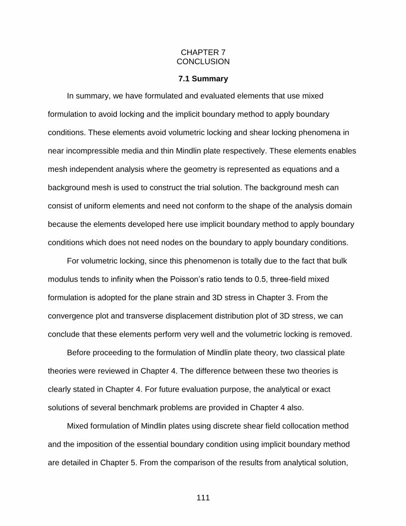
111
CHAPTER 7 CONCLUSION
7.1 Summary
In summary, we have formulated and evaluated elements that use mixed
formulation to avoid locking and the implicit boundary method to apply boundary
conditions. These elements avoid volumetric locking and shear locking phenomena in
near incompressible media and thin Mindlin plate respectively. These elements enables
mesh independent analysis where the geometry is represented as equations and a
background mesh is used to construct the trial solution. The background mesh can
consist of uniform elements and need not conform to the shape of the analysis domain
because the elements developed here use implicit boundary method to apply boundary
conditions which does not need nodes on the boundary to apply boundary conditions.
For volumetric locking, since this phenomenon is totally due to the fact that bulk
modulus tends to infinity when the Poisson’s ratio tends to 0.5, three-field mixed
formulation is adopted for the plane strain and 3D stress in Chapter 3. From the
convergence plot and transverse displacement distribution plot of 3D stress, we can
conclude that these elements perform very well and the volumetric locking is removed.
Before proceeding to the formulation of Mindlin plate theory, two classical plate
theories were reviewed in Chapter 4. The difference between these two theories is
clearly stated in Chapter 4. For future evaluation purpose, the analytical or exact
solutions of several benchmark problems are provided in Chapter 4 also.
Mixed formulation of Mindlin plates using discrete shear field collocation method
and the imposition of the essential boundary condition using implicit boundary method
are detailed in Chapter 5. From the comparison of the results from analytical solution,

112
exact solution, IBFEM element solution and Abaqus element analysis, the performance
of the IBFEM elements can be easily assessed. It is clear that these elements are
useful and robust, and at least as good as, if not better than, the elements from the
commercial package ABAQUS.
2D Mindlin shell, that includes in-plane stretching and transverse pressure, is also
studied in this thesis. From the results, these elements also perform well. The objective
of this extension of Mindlin plate is to prepare the formulation of general curved shell
elements using IBFEM.
In conclusion, we have successfully implemented the mixed formulation using
IBFEM so as to avoid volumetric locking and shear locking phenomena.
7.2 Scope of Future Work
The three-field mixed formulation we have employed in this thesis is only valid for
nearly incompressible media, since there is still bulk modulus term in the modified
stiffness matrix. Hence, in order to remove volumetric locking for completely
incompressible media, new finite element techniques should be used for this purpose.
Two-field ( u p ) mixed formulation is a possible way according to Hughes [9] and Bathe
[1].
The mixed formulation using discrete shear field collocation method and IBFEM is
developed in this thesis only for elastic static Mindlin plates. The validity of this method
is already evaluated in Chapter 5. Future work can extend this method to nonlinear and
dynamic analysis of Mindlin plates.
The mixed formulation of 2D Mindlin shell, including both in-plane stretching and
bending, is derived in Chapter 6. This can be viewed a special 2D case of shell

113
formulation. Hence, generalizing this method for 3D shell analysis can be a prospective
future direction.

114
APPDENDIX A VOLUMETRIC LOCKING AND SHEAR LOCKING
Volumetric locking and shear locking are the most common numerical phenomena
in the displacement-base finite element formulation. We will give some details in order
to better understand these two frequent phenomena in FEM.
A.1 Volumetric locking
Volumetric locking is very obvious as we already presented at the beginning of
Chapter 3. This phenomenon results from the fact that when the material is near
incompressible status, the Poisson’s ratio, v , tends to 0.5, which makes the bulk
modulus / (3 6 )E v tend to infinity and hence a ill-conditioned stiffness matrix in the
finite element model.
A.2 Shear locking
Shear locking is an error that occurs in finite element analysis. It can be explained
as following.
Let us consider a beam with thickness h under combined shear and bending
deformations. As we have done in Chapter 5, the total strain energy can be expressed
as
2
1 1
2 2
1
2
1 1
2 2
1 1[ ( ) ( )]
2 2
1 1( ) ( )
2 2
T T
stV h
kT
k Sh
S
T T
k k S Sh h
T T
S Sh
T T
S S
U dV dzd
dzdkG
dzd kG dzd
z dzd d
d d
ε Qε ε Qε
εC 0ε γ
γ0
ε Cε γ γ
C γ γ
D γ γ
(A-1)
Where

115
3
2
1 0
1 012 (1 )
0 0 (1 ) / 2
vh E
vv
v
D (A-2)
h G (A-3)
From (A-1), the portion of the strain energy associated with the bending
deformation is proportional to 3h , and the portion related to shear deformations is
proportional to h . If we reduce the thickness h , the value of 3h approaches to zero much
faster than h and as a result, the total strain energy of the beam will largely come from
shear deformation. This is not correct because for a thin beam it is always the bending
deformation which provides most part of the strain energy. So any shear strain resulting
from numerical errors and due to the use of low order shape functions can lead to
wrong results for very thin beam, small displacement.

116
APPENDIX B EQUILIBRIUM EQUATIONS OF 3D ELASTOSTATIC CASE
Figure B-1. Stresses notations and directions
Comparing to these stresses, the body force is of high order, so we neglect it in
above figure B-1. But in the process of deriving the equilibrium equation, we should take
the body force into consideration, since it’s the same order as the variation terms of
stresses.
The equation of equilibrium of force in the x-direction is
' ' ' 0zxyxx x yx zx xdxdydzdydz dydz dxdz dxdz dxdy dxdy b (B-1)
Dividing by dxdydz ,
'' '
0yxx zxyxx zx
xdx dy dz
b
(B-2)
If the block is become smaller and smaller, i.e.,
0, 0, 0dx dy dz (B-3)
By definition of derivative, we have

117
'
0lim x
dx
x x
dx x
(B-4)
'
0limdy
yx yx yx
dy y
(B-5)
'
0limdz
zx zx zx
dz z
(B-6)
Plugging B-4 to B-6 into B-2, we have the first differential equilibrium equation as
0yxx zx
xbx y z
(B-7)
Using the same manner, we can derive the left two equations as
0xy y zy
ybx y z
(B-8)
0yzxz z
zbx y z
(B-9)

118
APPENDIX C DERIVATION OF SHEAR CORRECTION FACTOR
The transverse shear correction coefficient can be derived using equivalence of
shear strain energy before and after using this factor.
Equivalence of Shear strain energy
The first two equilibrium equations of a static case without body force are
0xyx xz
x y z
(C-1)
0xy y yz
x y z
(C-2)
Integrating C-1 and C-2, we can obtain the transverse stress at any point through
the thickness as
/2/2
( )
z
xz
h
xyxxz h
dzx y
(C-3)
/2/2
( )
z
yz
h
xy y
yzh
dzx y
(C-4)
/2xz h
and
/2yz
h
are the shear stresses at the bottom of the plate and both are
equal to zero.
Given the in-plane strains, the in-plane stresses can be obtained using the stress-
strain relationship as
11 12 11 12
12 22 12 22
33 33
0 0
0 0
0 0 0 0
)(
x
x xy
y y
xy xy
yx
C C C C
C C C C
C C
zx
zy
zy x
(C-5)

119
Substituting Equation C-5 into Equations C-3 and C-4, and performing the
integration, we obtain the following results
2 22 22 2
11 12 332 2 2
4[ ( )](1 )
8
y yx xxz
h zC C C
x x y y x y h
(C-6)
2 22 22 2
33 22 122 2 2
4[ ( ) ](1 )
8
y yx xyz
h zC C C
x y x y x y h
(C-7)
For rectangular plate, the transverse stresses parabolically vary through the
thickness h .
Figure C-1. Distribution of transverse shear stress through the thickness
In Equations C-6 and C-7, we have following relations
22
11 12 11 122 3
22
33 332 3
2 2
22 12 22 122 3
22
33 332
12( )
12( ) ( ( ))
12( )
( ) ( (
y yx x x
y y xyx x
y y yx x
yx x
MC C C C
x x y x x y h x
MC C
y x y y y x h y
MC C C C
y x y y y x h y
C Cx y x x y
3
12))
y xyM
x h x
(C-8)
Thus, xz and yz can be further expressed as
2
2
3 4[ ](1 )
2
xyxxz
MM z
h x y h
(C-9)

120
2
2
3 4[ ](1 )
2
y xy
yz
M M z
h y x h
(C-10)
From Equation C-8, C-9 and C-10, we finally have
2
2
3 4(1 )
2xz x
zS
h h
(C-11)
2
2
3 4(1 )
2yz y
zS
h h (C-12)
Generally, the total strain energy per unit area due to transverse shears is
2/2 /2 2
/2 /2
1 1( ) ( )
2 2
h hyzxz
xz xz yz yzSAh h
U dz dzG G
(C-13)
Plugging Equations C-11 and C-12 into Equation C-13, we have
2 21 6( )
2 5x ySA S S
G hU (C-14)
In shear deformable plate theory, we assumed at the beginning that
xz xz
yzyz
SGhS
(C-15)
Hence, we also have the total strain energy per unit area due to transverse shears
as
2 21 1( ) ( )
2 2SA xz xz yz yz xz yzS S S S
GhU
(C-16)
Comparing Equation C-14 and Equation C-16 for total strain energy due to the
same transverse shears, we have
5
6 (C-17)

121
APPENDIX D DERIVATION OF THE JACOBIAN MATRIX IN IBFEM
The Jacobian matrix for 2D is in the format as following:
x y
x y
J (D-1)
We can modified above expression for J of 9-node element as
9 9
1 19 9
1 1
1 2 3 4 5 6 7 8 9
1 2 3 4 5 6 7 8 9
I I
w wI I
eI I
w wI I
w w w w w w w w w
w w w w w w w w w
N Nx yx y
x y N Nx y
N N N N N N N N N
N N N N N N N N N
J
1 1
2 2
3 3
4 4
5 5
6 6
7 7
8 8
9 9
x yx yx yx yx yx yx yx yx y
(D-2)
In IBFEM, we have following relations
1 8 4 1 5 9 7 2 2 6 3 3
1 5 2 1 8 9 6 2 4 7 3 3
2 1 3
2 1 3
, ,
, ,
2
2
x x x X x x x X x x x X
y y y Y y y y Y y y y Y
Y Y Y
X X X
(D-3)
Using these relations in above expression for J , we can get
1 3
1 3
02
02
X X
Y Y
J (D-4)

122
Figure D-1. Global coordinate and Local coordinate in IBFEM

123
APPENDIX E FORMULATION OF MINDLIN PLATE ELEMENTS
E.1 Element Q4D4
Figure E-1. Collocation constraints on a 4-node Lagrange element
Shape function for displacement and rotations
The shape functions for rotation are the same as those for the displacement with
corresponding node.
These shape functions for displacement are
1 2
3 4
1 1(1 )(1 ), (1 )(1 ),
4 4
1 1(1 )(1 ), (1 )(1 ),
4 4
w w
w w
N N
N N
(E-1)
The shape functions for rotations are
1 1 1 2 1 2
3 1 3 4 1 4
, ,
, ,
x y w x y w
x y w x y w
N N N N N N
N N N N N N
(E-2)
Shape function for shear fields

124
The shape functions for shear fields can be derived using the same structure of
Lagrange polynomials. And these shape functions are
1 1 2 2
3 3 4 4
1 1, 0, 0, ,
2 2
1 1, 0, 0, ,
2 2
s s s s
s s s s
N N N N
N N N N
(E-3)
Derivation of the prescribed shear force value
Figure E-2. Interpolation nodes for Q4D4 element
For above Q4D4 element, the displacement and the rotation can be approximated
as ˆwwN w and ˆ
N
Using
ˆ ˆˆ ˆ( , )
ˆ ˆˆ ˆ( , )
w wx
w wy
Sx x
Sy y
N Nw N w N
N Nw N w N
, (E-4)
we can derive the prescribed values for shear force at certain nodes using prescribed w
and as

125
1 4
3 4
1 22 1
01
1 4
10
3
01
2
ˆ ˆ
2
ˆ ˆ
2
ˆ ˆˆ ˆˆ ˆˆ [( ) ]2
ˆ ˆˆ ˆˆ [( ) ]
2
ˆˆ ˆˆ [( )
I w x xx
y yII wy
III w xx
w w
w w
w wS
x x
Sy y
Sx x
Nw N
Nw N
Nw N
2 3
4
2 3
10
ˆ ˆ
2
ˆ]
2
ˆ ˆˆ ˆˆ [( ) ]
2
x
y yIV wy
w wS
y y
Nw N
(E-5)
Where N , N , ˆ and ˆ
are the and components of N and .
In IBFEM, we have
2
2
x a
y b
, where a andb are the length of edges of an element
in x and y direction, respectively.
Writing in the matrix form, we have
ˆ ˆˆw
S Q w Q
where
ˆ ˆ ˆ ˆ ˆT
I II III IV
x y x yS S S SS (E-6)
0 0
0 0
0 0
0 0
1 1
1 1
1 1
1 1
w
a a
b b
a a
b b
Q (E-7)

126
1 0 1 0 0 0 0 0
0 1 0 0 0 0 0 11
0 0 0 0 1 0 1 02
0 0 0 1 0 1 0 0
Q (E-8)
The same procedure is used to get the collocated shear term and its shape
function, and we will not give more details in the following content about the derivation
for each element. And also, the shape functions for the displacement are the same as
traditional ones. The shape functions for rotations are the same as those of
displacement at the corresponding nodes.
E.2 Element Q5D6
Figure E-3. Collocation constraints on a 5-node Serendipity element
Shape function for shear fields
1 1 2 2
3 3 4 4
5 5 6 6
( 1) ( 1), 0, 0, ,
2 2
( 1) ( 1), 0, 0, ,
2 2
( 1)( 1), 0, 0, ( 1)( 1),
s s s s
s s s s
s s s s
N N N N
N N N N
N N N N
(E-9)

127
Figure E-4. Interpolation nodes for Q5D6 element
wQ and Q matrices
ˆ ˆ ˆ ˆ ˆ ˆ ˆT
I II III IV V VI
x y x y x yS S S S S SS (E-10)
0 0 0
0 0 0
0 0 0
0 0 0
0
0
1 1
1 1
1 1
1 1
1 1 1 1
2 2 2 2
1 1 1 1
2 2 2 2
w
a a
b b
a a
b b
a a a a
b b b b
Q (E-11)
1 0 1 0 0 0 0 0 0 0
0 0 0 1 0 1 0 0 0 0
0 0 0 0 1 0 1 0 0 01
0 1 0 0 0 0 0 1 0 02
0 0 0 0 0 0 0 0 2 0
0 0 0 0 0 0 0 0 0 2
Q (E-12)

128
E.3 Element Q8D8
Figure E-5. Collocation constraints on an 8-node Serendipity element
Shape functions for shear fields
1 1 2 2
3 3 4 4
5 5 6 6
7 7 8 8
1 1 1 1( )( 1), 0, ( )( 1), 0,
2 2 2 2
1 1 1 10, ( 1)( ), 0, ( 1)( ),
2 2 2 2
1 1 1 1( )( 1), 0, ( )( 1), 0,
2 2 2 2
1 1 10, ( 1)( ), 0,
2 2 2
s s s s
s s s s
s s s s
s s s s
N N N N
N N N N
N N N N
N N N N
1
( 1)( ),2
(E-13)
Figure E-6. Interpolation nodes for Q8D8 element
wQ and Q matrices

129
ˆ ˆ ˆ ˆ ˆ ˆ ˆ ˆ ˆT
I II III IV V VI VII VIII
x x y y x x y yS S S S S S S SS (E-14)
0 0 0 0 0 0
0 0 0 0 0
0 0 0 0 0 0
0 0 0 0
0 0 0 0 0 0
0 0 0 0 0 0
0 0 0 0
0 0 0 0 0 0
1 1
1 10
1 1
1 10 0
21 1
1 1
1 10 0
1 1
w
a a
a a
b b
b b
a a
a a
b b
b b
Q (E-15)
3 0 1 0 0 0 0 0 6 0 0 0 0 0 0 0
1 0 3 0 0 0 0 0 6 0 0 0 0 0 0 0
0 0 0 3 0 1 0 0 0 0 0 6 0 0 0 0
0 0 0 1 0 3 0 0 0 0 0 6 0 0 0 01
0 0 0 0 3 0 1 0 0 0 0 0 6 0 0 08
0 0 0 0 1 0 3 0 0 0 0 0 6 0 0 0
0 1 0 0 0 0 0 3 0 0 0 0 0 0 0 6
0 3 0 0 0 0 0 1 0 0 0 0 0 0 0 6
Q (E-16)

130
E.4 Element Q9D12
Figure E-7. Collocation constraints on a 9-node Lagrange element
Shape functions for shear fields
1 1 2 2
3 3 4 4
5 5 6 6
1 1 1 1( ) ( 1), 0, ( ) ( 1), 0,
2 2 2 2
1 1 10, ( 1)( ), 0, ( 1)( 1)( ),
2 2 2
1 1 10, ( 1)( ), ( )( 1)( 1), 0,
2 2 2
s s s s
s s s s
s s s s
N N N N
N N N N
N N N N
(E-17)
7 7 8 8
9 9 10 10
11 11 12 12
1 1 1( )( 1)( 1), 0, 0, ( 1)( ),
2 2 2
1 1 10, ( 1)( 1)( ), 0, ( 1)( ),
2 2 2
1 1 1 1( ) ( 1), 0, ( ) ( 1), 0,
2 2 2 2
s s s s
s s s s
s s s s
N N N N
N N N N
N N N N
(E-18)
wQ and Q matrices

131
Figure E-8. Interpolation nodes for Q9D12 element
ˆ ˆ ˆ ˆ ˆ ˆ ˆ ˆ ˆ ˆ ˆ ˆ ˆT
I II III IV V VI VII VIII IX X XI XII
x x y y y x x y y y x xS S S S S S S S S S S SS (E-19)
1
8
1 0 3 0 0 0 0 0 6 0 0 0 0 0 0 0 0 0
3 0 1 0 0 0 0 0 6 0 0 0 0 0 0 0 0 0
0 0 0 3 0 1 0 0 0 0 0 6 0 0 0 0 0 0
0 0 0 0 0 0 0 0 0 3 0 0 0 1 0 0 0 6
0 3 0 0 0 0 0 1 0 0 0 0 0 0 0 6 0 0
0 0 0 0 0 0 0 0 0 0 3 0 0 0 1 0 6 0
0 0 0 0 0 0 0 0 0 0 1 0 0 0 3 0 6 0
0 0 0 1 0 3 0 0 0 0 0 6 0 0 0 0 0 0
0 0 0 0 0 0 0 0 0 1 0 0 0 3 0 0 0 6
0 1 0 0 0 0 0 3 0 0 0 0 0 0 0 6 0 0
0 0 0 0 3
Q
0 1 0 0 0 0 0 6 0 0 0 0 0
0 0 0 0 1 0 3 0 0 0 0 0 6 0 0 0 0 0
(E-20)

132
0 0 0 0 0 0 0
0 0 0 0 0 0 0
0 0 0 0 0 0 0
0 0 0 0 0 0 0
0 0 0 0 0 0 0
0 0 0 0 0 0 0
0 0 0 0 0 0 0
0 0 0 0 0 0 0
0 0 0 0 0 0 0
0 0 0 0 0 0 0
0 0 0 0 0 0 0
0 0 0 0 0 0 0
1 1
1 1
1 1
1 1
1 1
1 1
21 1
1 1
1 1
1 1
1 1
1 1
w
a a
a a
b b
b b
b b
a a
a a
b b
b b
b b
a a
a a
Q
(E-21)
E.5 Element Q16D24
Figure E-9. Collocation constraints on a 16-node Lagrange element
Shape function for shear fields

133
1 1
2 2
3 3
4 4
5 5
81 1 1 2( )( )( 1) ( ), 0,
128 3 3 3
81 1 1 2 2( )( )( 1)( )( ), 0,
64 3 3 3 3
81 1 1 2( )( )( 1) ( ), 0,
128 3 3 3
81 1 1 20, ( )( )( 1) ( ),
128 3 3 3
81 1 10, ( )(
64 3
s s
s s
s s
s s
s s
N N
N N
N N
N N
N N
6 6
2 2)( 1)( )( ),
3 3 3
81 1 1 20, ( )( )( 1) ( ),
128 3 3 3s sN N
(E-22)
7 7
8 8
9 9
10 10
11 11
81 1 1 2( )( )( 1) ( ), 0,
128 3 3 3
81 1 1 2 2( )( )( 1)( )( ), 0,
64 3 3 3 3
81 1 1 2( )( )( 1) ( ), 0,
128 3 3 3
81 1 1 20, ( )( )( 1) ( ),
128 3 3 3
81 10, (
128
s s
s s
s s
s s
s s
N N
N N
N N
N N
N N
12 12
1 2 2)( )( 1)( )( ),
3 3 3 3
81 1 1 20, ( )( )( 1) ( ),
128 3 3 3s sN N
(E-23)
13 13
14 14
15 15
16 16
17 17
243 1 20, ( )( 1)( 1) ( ),
128 3 3
243 1 20, ( )( 1)( 1) ( ),
128 3 3
243 1 2( )( 1)( 1) ( ), 0,
128 3 3
243 1 2( )( 1)( 1) ( ), 0,
128 3 3
2430, (
128
s s
s s
s s
s s
s s
N N
N N
N N
N N
N N
18 18
1 2)( 1)( 1) ( ),
3 3
243 1 20, ( )( 1)( 1) ( ),
128 3 3s sN N
(E-24)

134
19 19
20 20
21 21
22 22
23
243 1 2( )( 1)( 1) ( ), 0,
128 3 3
243 1 2( )( 1)( 1) ( ), 0,
128 3 3
243 1 2 2( )( 1)( 1)( )( ), 0,
64 3 3 3
243 1 2 20, ( )( 1)( 1)( )( ),
64 3 3 3
243(
64
s s
s s
s s
s s
s
N N
N N
N N
N N
N
23
24 24
1 2 2)( 1)( 1)( )( ), 0,
3 3 3
243 1 2 20, ( )( 1)( 1)( )( ),
64 3 3 3
s
s s
N
N N
(E-25)
wQ and Q matrices
ˆ ˆ ˆ ˆ ˆ ˆ ˆ ˆ ˆ ˆ ˆ ˆˆ
ˆ ˆ ˆ ˆ ˆ ˆ ˆ ˆ ˆ ˆ ˆ ˆ
TI II III IV V VI VII VIII IX X XI XII
x x x y y y x x x y y yXIII XIV XV XVI XVII XVIII XIX XX XXI XXII XXIII XXIV
y y x x y y x x x y x y
S S S S S S S S S S S S
S S S S S S S S S S S S
S (E-26)
23 / 1 / 0 0 21 / 3 / 0 0 0 0 0 0 0 0 0 0
1 / 1 / 0 0 27 / 27 / 0 0 0 0 0 0 0 0 0 0
1 / 23 / 0 0 3 / 21 / 0 0 0 0 0 0 0 0 0 0
0 23 / 1 / 0 0 0 21 / 0 0 0 3 / 0 0 0 0 0
0 1 / 1 / 0 0 0 27 / 0 0 0 27 / 0 0 0 0 0
0 1 / 23 / 0 0 0 3 / 0 0 0 21 / 0 0 0 0 0
0 0 23 / 1 / 0 0 0 0 0 0 0 0 0 0 21 / 3 /
1
8w
a a a a
a a a a
a a a a
b b b b
b b b b
b b b b
a a a
Q
0 0 1 / 1 / 0 0 0 0 0 0 0 0 0 0 27 / 27 /
0 0 1 / 23 / 0 0 0 0 0 0 0 0 0 0 3 / 21 /
1 / 0 0 23 / 0 0 0 0 0 3 / 0 0 0 21 / 0 0
1 / 0 0 1 / 0 0 0 0 0 27 / 0 0 0 27 / 0 0
23 / 0 0 1 / 0 0 0 0 0 21 / 0 0 0 3 / 0 0
0 0 0 0 23 / 0 0 0 21 / 0 0 0 3 / 0 0 1 /
0 0 0 0 0 23 / 0 21 / 0 0 0 3 / 0 0 1 / 0
0 0 0
a
a a a a
a a a a
b b b b
b b b b
b b b b
b b b b
b b b b
0 0 0 23 / 21 / 3 / 1 / 0 0 0 0 0 0
0 0 0 0 0 0 0 0 0 0 23 / 21 / 3 / 1 / 0 0
0 0 0 0 0 1 / 0 3 / 0 0 0 21 / 0 0 23 / 0
0 0 0 0 1 / 0 0 0 3 / 0 0 0 21 / 0 0 23 /
0 0 0 0 0 0 0 0 0 0 1 / 3 / 21 / 23 / 0 0
0 0 0 0 0 0 1 / 3 / 21 / 23 / 0 0 0 0 0 0
0 0 0 0 0 0 1 / 27 / 27 / 1 / 0 0 0 0 0 0
0 0 0 0 0 1
a a a a
a a a a
b b b b
b b b b
a a a a
a a a a
a a a a
/ 0 27 / 0 0 0 27 / 0 0 1 / 0
0 0 0 0 0 0 0 0 0 0 1 / 27 / 27 / 1 / 0 0
0 0 0 0 1 / 0 0 0 27 / 0 0 0 27 / 0 0 1 /
b b b b
a a a a
b b b b
(E-27)

135
5 0 1 0 0 0 0 0 15 0 5 0 0 0 0 0 0 0 0 0 0 0 0 0 0 0 0 0 0 0 01 0 1 0 0 0 0 0 9 0 9 0 0 0 0 0 0 0 0 0 0 0 0 0 0 0 0 0 0 0 0
1 0 5 0 0 0 0 0 5 0 15 0 0 0 0 0 0 0 0 0 0 0 0 0 0 0 0 0 0 0 00 0 0 5 0 1 0 0 0 0 0 0 0 15 0 0 0 0 0 0 0 5 0 0 0 0 0 0 0 0 00 0 0 1 0 1 0 0 0 0 0 0 0 9 0 0 0 0 0 0 0 9 0 0 0 0 0 0 0 0 00 0 0 1 0 5 0 0 0 0 0 0 0 5 0 0 0 0 0 0 0 15 0 0 0 0 0
1
16
Q
0 0 0 00 0 0 0 5 0 1 0 0 0 0 0 0 0 0 0 0 0 0 0 0 0 0 0 0 0 0 0 15 0 50 0 0 0 1 0 1 0 0 0 0 0 0 0 0 0 0 0 0 0 0 0 0 0 0 0 0 0 9 0 90 0 0 0 1 0 5 0 0 0 0 0 0 0 0 0 0 0 0 0 0 0 0 0 0 0 0 0 5 0 150 1 0 0 0 0 0 5 0 0 0 0 0 0 0 0 0 0 0 5 0 0 0 0 0 0 0 15 0 0 00 1 0 0 0 0 0 1 0 0 0 0 0 0 0 0 0 0 0 9 0 0 0 0 0 0 0 9 0 0 00 5 0 0 0 0 0 1 0 0 0 0 0 0 0 0 0 0 0 15 0 0 0 0 0 0 0 5 0
0 0
0 0 0 0 0 0 0 0 0 5 0 0 0 0 0 0 0 15 0 0 0 0 0 0 0 5 0 0 0 0 00 0 0 0 0 0 0 0 0 0 0 5 0 0 0 15 0 0 0 0 0 0 0 5 0 0 0 0 0 1 00 0 0 0 0 0 0 0 0 0 0 0 5 0 15 0 5 0 1 0 0 0 0 0 0 0 0 0 0 0 00 0 0 0 0 0 0 0 0 0 0 0 0 0 0 0 0 0 0 0 5 0 15 0 5 0 1 0 0 0 00 0 0 0 0 0 0 0 0 0 0 1 0 0 0 5 0 0 0 0 0 0 0 15 0 0 0 0 0 5 00 0 0 0 0 0 0 0 0 1 0 0 0 0 0 0 0 5 0 0 0 0 0 0 0 15 0 0 0 0 0
000
0 0 0 0 0 0 0 0 0 0 0 0 0 0 0 0 0 0 0 0 1 0 5 0 15 0 5 0 0 0 00 0 0 0 0 0 0 0 0 0 0 0 1 0 5 0 15 0 5 0 0 0 0 0 0 0 0 0 0 0 00 0 0 0 0 0 0 0 0 0 0 0 1 0 9 0 9 0 1 0 0 0 0 0 0 0 0 0 0 0 00 0 0 0 0 0 0 0 0 0 0 1 0 0 0 9 0 0 0 0 0 0 0 9 0 0 0 0 0 1 00 0 0 0 0 0 0 0 0 0 0 0 0 0 0 0 0 0 0 0 1 0 9 0 9 0 1 0 0 0 00 0 0 0 0 0 0 0 0 1 0 0 0 0 0 0 0 9 0 0 0 0 0 0 0 9 0 0 0 0 0
000000000100005000001
(E-28)
Figure E-10. Interpolation nodes for Q16D24 element

136
LIST OF REFERENCES
[1] Bathe, K.J. (1996). Finite Element Procedures, 2nd ed., Prentice-Hall, New Jersey.
[2] Bathe, K.J., Dvorkin, E.N. (1985). A four-node plate bending element based on Mindlin/Reissner plate theory and a mixed interpolation. International Journal of Numerical Methods in Engineering, 21(2), 367-383.
[3] Belytschko, T., Krongauz, Y., Organ, D., Fleming, M., Krysl, P. (1996). Meshless Methods: An Overview and Recent Developments. Computer Methods in Applied Mechanics and Engineering, 139, 3-47.
[4] Belytschko, T., Parimi, C., Moes, N., Usui, S., Sukumar, N. (2003). Structured extended finite element methods for solids defined by implicit surfaces. International Journal for Numerical Methods in Engineering, 56(4), 609-635.
[5] Clark, B.W., Anderson, D.C. (2002). Finite Element Analysis in 3D Using Penalty Boundary Method. Proceedings of Design Engineering Technical Conferences, Montreal, Canada.
[6] Fish, J., Belytschko, T. (2007). A first course in finite elements, John Wiley and Sons.
[7] Hinton, E., Huang, H.C. (1986). A family of quadrilateral Mindlin plate elements with substitute shear strain fields. Computers and Structures, 23 (3), 409-431.
[8] Hrabok, M.M., Hrudey, T.M. (1984). A review and catalogue of plate bending finite elements. Computers and Structures, 19(3), 479-495.
[9] Hughes, T.J.R. (2000). The Finite Element Method: Linear Static and Dynamic Finite Element Analysis, 2nd edition. Dover Editions, New Jersey.
[10] Kantorovich, L.W., Krylov, W.I. (1956). Näherungsmethoden der Höheren Analysis. VEB Deutscher Verlag der Wissenschaften, Berlin.
[11] Kumar, A.V., Burla, R., Padmanabhan, S., Gu, L. (2008). Finite element analysis using nonconforming mesh. Journal of Computing and Information Science in Engineering, 8, 031005-1.
[12] Kumar, A.V., Lee, J. (2003). Step function representation of solid models and application to mesh free engineering analysis, Journal of Mechanical Design. Transactions of the ASME, 128(1), 46-56.
[13] Kumar, A.V., Padmanabhan, S., Burla, R. (2008). Implicit boundary method for finite element analysis using non-conforming mesh or mesh. International Journal for Numerical Methods in Engineering, 74 (9), 1421-1447.

137
[14] Liew, K.M., Han, J.-B. (1997). Bending analysis of simply supported shear deformable skew plates. Engineering Mechanics, 123(3), 214-221.
[15] Rvachev, V.L., Shieko, T.I. (1995). R-functions in Boundary Value Problems in Mechanics. Applied Mechanics Review, 48, 151-188.
[16] Sengupta, D. (1995). Performance study of a simple finite element in the analysis of skew rhombic plates. Computers and Structures, 54 (6), 1173-1182.
[17] Taylor, R.L., Govindjee, S. (2004. )Solution of clamped rectangular problems. Communications in Numerical Methods in Engineering. 20, 757-765.
[18] Timoshenko, S., Woinowsky-Kreiger, S. (1987). Theory of Plates and Shells, second edition. McGraw-Hill, New York.
[19] Wang, C.M., Reddy, J.N., Lee, K.H. (2000). Shear Deformable Beams and Plates: Relationships with Classical Solutions. Elsevier, Oxford.
[20] Yang, T.Y., Saigal, S., Masud, A., Kapania, R.K. (2000). A survey of recent shell finite elements. International Journal for Numerical Methods in Engineering, 47, 101-127.
[21] Zienkiewicz, O.C., Taylor, R.L., Zhu, J.Z. (2005). The Finite Element Method for Solid and Structural Mechanics, sixth edition. Butterworth-Heinemann.
[22] Zienkiewicz, O.C., Xu, Z., Zeng, L.F., Samuelson, Wilbert, N.E. (1993). Linked interpolation for Reissner – Mindlin plate elements: Part I - A simple quadrilateral. International Journal for numerical Methods in Engineering, 36, 3043 – 3056.

138
BIOGRAPHICAL SKETCH
Hailong Chen was born and brought up in Jiangxi, China. He graduated with a
Bachelor of Science in engineering degree in mechanical engineering from Shanghai
Normal University, Shanghai, China in June 2010 with honors. After graduation, he
directly enrolled in the master’s program in Mechanical and Aerospace Engineering at
the University of Florida in fall 2010 with Achievement Award for New Engineering
Graduate Students. In 2011, he and Xiao Zhou got married in China. His area of interest
includes application of FEM in plates and shells, numerical methods and uncertainty
quantification.