Embed Size (px)
Citation preview

AUTOMATIC TIMEISERIES MODEL GENERATION FOR REAL-TIME
STATISTICAL PROCESS CONTROL
by
Hao-Cheng Liu
Memorandum No. UCBBRL M93/45
8 June 1993


AUTOMATIC TIME-SERIES MODEL GENERATION FOR REAL-TIME
STATISTICAL PROCESS CONTROL
by
Hao-Cheng Liu
Memorandum No. UCBERL M93/45
8 June 1993


AUTOMATIC TIME-SERIES MODEL GENERATION FOR REAL-TIME
STATISTICAL PROCESS CONTROL
by
Hao-Cheng Liu
Memorandum No. UCBERL M93/45
8 June 1993
ELECTRONICS RESEARCH LABORATORY
College of Engineering University of California, Berkeley
94720

To my father, my mother and Stephanie 1 for their love and support.

Acknowledgment I
I would like to express my deep appreciation and gratitude to my research advisor, Dr.
Costas J. Spanos, for his support and guidance through my graduate studies an the latter 9 portion of my undergraduate studies. I also thank Dr. John A. Rice for being
project report committee and for his valuable insights in time-series modeling.
Special thanks are due to two colleagues in the BCAM group: Mr. Eddie
work in developing the BCAM Real-Time SPC interface, and Ms. Sherry
her knowledge and expertise and providing insightful feedbacks and
help and friendship are greatly appreciated.
I would also like to extend my gratitude to the rest of the BCAM group for making my
graduate experience an enjoyable one. They are Mr. Eric Boskin, Mr. Eric Braun, Mr.
Raymond Chen, Mr. Sean Cunningham, Ms. Zeina Daoud, Mr. Kwan Kim, Mr. Sovarong
Leang, Ms. Pamela Tsai, and Mr. Crid Yu. Special thanks are also extended to past BCAM
members Mr. Bart Bombay, Ms. Haifang Guo, Ms. Lauren Massa-Lochridge, Mr. Tom
Luan, Dr. Gary May, and Mr. John Thompson.
I am also grateful to the Semiconductor Research Corporation and International Busi-
ness Machines Corporation for sponsoring this work.

i
AUTOMATIC TIME-SERIES MODEL GENERATION FOR REAL-TIME
STATISTICAL PROCESS CONTROL
by Hao-Cheng Liu
ABSTRACT
As integrated circui; designs become more complex, in compliance with Mdore’s h w ,
assuring the production quality of these complex integrated circuits becomes increasingly
difficult. Consequently, semiconductor manufacturers must focus on achieving tighter
real-time process control in order to obtain justifiable production yields as well as sustain
profitability in an increasingly competitive marketplace.
Traditionally, equipment and process faults are being discovered by “in-line”
measurements done between process steps. However, due to an increased pressure to
produce of a highly diverse product mixture in shorter cycle times, equipment and process
faults must be detected in real-time. However, because real-time process contrbl requires
the analysis of real-time equipment sensor data, traditional statistical process control
(SPC) techniques [ 13 cannot be readily applied to the sensor data due to their non-
stationary, auto-correlated and cross-correlated characteristics.
The Berkeley Computer-Aided Manufacturing (BCAM) Real-Time SplC system
utilizes econometric time-series models [2] in order to filter real-time readiqgs of any
existing autocorrelations. In addition, multivariate statistics, in particular, the Hotelling’s
TL statistic [3], are then used in order to combine the various cross-correlated signals into
a single statistical score. This T2 statistic is monitored with a single-sided contr
real-time SPC [4].

The objective of this project was to develop and implement an algorithm
automating the time-series model generation process for real-time SPC. Furthermore,
modifications must be made to the real-time SPC scheme in order to accomodate the batch
nature of single-wafer processing operations. As a result, the BCAM Real-Time SPC
scheme has been modified, and an automatic time-series model generator has beem
developed. The model generator has demonstrated success in generating useful time-series
models for real-time sensor data filtering. Furthermore, the modified SPC scheme, which
involves generating separate T2 statistics for detecting withimwafer and wafer-fo-wajiir
faults, has shown to be superior in detecting processing faults than the originally proposed
methodology, .
Signature: /
Professor Costas J . Spanos Committee Chairman
for
_-
Table of Contents
Chapter 1 Introduction 1.1 Background 1.2 Motivation 1.3 Organization
Chapter 2 The BCAM Real-Time SPC 2.1 Overview 2.2 Problems
Chapter 3 Automatic Time-Series Model Generation 3.1 Background 3.2 Stationarity and Time-Series Integration 3.3 The Yule-Walker Equations and AR Modeling 3.4 The Modified Yule-Walker Equations and ARMA
Modeling 3.5 Modifications to Time-Series Model Generation
Algorithm for Noise Compensation 3.6 Summary
Chapter 4 Modified Real-Time SPC with Automatic Time-Series Model Generation 4.1 Overview of Modifications 4.2 Within-Wafer Data Modeling and Filtering 4.3 Wafer-to-Wafer Data Modeling and Filtering 4.4 The Double-T2 Control Chart 4.5 Summary
Chapter 5 Implementation and Experimental Results 5.1 Implementation
5.1.1 The BCAM Real-Time SPC System 5.1.2 Automatic ARMA Time-Series Model Generator
5.2.1 Summary of Experiment 5.2.2 Within-Wafer Residuals 5.2.3 Wafer- to- W afer Residuals 5.2.4 The Double-T2 Control Chart 5.2.5 Results
5.2 Experimental Results
1 1 2 3 4 4 8
12 12 13 17
20
23 25
26 26 27 29 30 32 34 34 34 37
, 38 38 41 43 44 45
Chapter 6 Conclusions and Future Work 46


Chapter
1.1 Background
1 Introduction
Currently, various statistical process control (SPC) techniques are being uised in the
industry in order to detect equipment or process faults that might be detrimental to the
product. The most common SPC approach is to use in-line data measured at the end of
each process step and to place this data on a traditional Shewhart Control Chart. This of
course assumes that the data is identically, independently and normally dismbuted (IIND)
around a constant mean p with a constant standard deviation (3 [ 11.
However, as semiconductor manufacturing processes become increasingly complex
and as production volume increases, it becomes imperative that equipment arld process
faults be detected online (during the wafer run) instead of in-line (after the wafer run).
Therefore equipment manufacturers begin to realize the importance of building machines
that are capable of monitoring sensor data on a real-time basis. These real-time sensor
readings, however, cannot be placed directly on a traditional control chart because of their
non-stationary, auto-correlated and cross-correlated characteristics.
Time-series models can be used to filter non-stationary and auto-correla
signals. The residuals coming out of these filters should be IIND. If the
uncorrelated, then each can be placed on a traditional Shewhan Control Chart.

2 Introduction Chap4r 1
The Berkeley Computer-Aided Manufacturing (BCAM) Real-Time SPC mod-ile
utilizes Seasonal Autoregressive Integrated Moving Average (SARIMA) time-ser:
models [2] for the filtration of the real-time sensor data. Because the filtered sensor
tend to be highly cross-correlated, multivariate statistics, in particular, the Hotelling’s
statistic [3], is used in order to combine the various cross-correlated signal residuals into
single statistical score. This T2 statistic is then placed on a single-sided control chart
real-time SPC [4].
1.2 Motivation
Currently, ARIMA time-series models for the BCAM Real-Time SPC module, as
as for other applications, are generated interactively using standard statistical analyijis
tools. This procedure is time-consuming and requires specialized skills in time-seri
statistics. An automated time-series model generator will make the BCAM Real-Time
SPC module, as well as several other advanced computer-aided manufacturi.?g
applications, more robust and practical.
Furthermore, there is a realization that SARIMA models, although used successfully,
may not be ideal, or proper, for modeling semiconductor equipment sensor signals. These
signals usually have only a small time segment of useful information from each wafer
SPC purposes. When one concatenates these small segments of data, the resulting tirne
series will no longer be continuous. However, the ARIMA time-series model can
modified so that separate models can be generated for detecting within-wafer as well
wafer-to-wafer time-series patterns, thus accommodating for the lack of continuity in t
concatenated sensor data. This modification must be built in to the proposed time-series
model generator in order to make the BCAM Real-lime SPC complete.
A modified real-time SPC scheme with automatic time-series model generation
been developed and applied on the Lam Research Rainbow single-wafer plasma etchcr.
es
drita
T 2
a
for
well
es
for
>e
as
le
has
Chapter 1 Introduction 3
The model generation algorithm has demonstrated success in generating useful tibe-series
models for filtering the real-time sensor data. Furthermore, the modified real-time SPC
scheme, which involves generating separate T2 statistics for detecting wirhin-wafer and
wafer-to-wafer faults, has proven to be superior in detecting processing fault4 than the
originally proposed methodology.
1.3 Organization
The BCAM Real-Time SPC scheme will be reviewed in Chapter 2. Char
introduce the readers to ARIMA time-series modeling, as well as to the tf
!er 3 will
eory and
algorithm for generating these models automatically. Modifications to the BCAM Real-
Time SPC system will be discussed in Chapter 4, along with the necessary modifications
to the automatic time-series model generation algorithm. Chapter 5 contains details in
regards to the implementation of the new BCAM Real-Time SPC system. Some
experimental results will then be presented in Chapter 6. The report will conclude in
Chapter 7 with a discussion about the effectiveness of the scheme and a proposal of future
work.

Chapter 2 The BCAM Real-Time SPC
2.1 Overview
Although the most popular methods for SPC involve the use of the traditional Shew
control chart or the cumulative sum (CUSUM) chart, these methods cannot be rea
applied to rapid, real-time readings. This is because these methods assume that the
being applied to these control charts are identically, independently and norm,
distributed (IIND), which typically is not the case with rapidly collected, real-t
equipment sensor data.
The Berkeley Computer-Aided Manufacturing (BCAM) Real-Time SPC scheme
attempts to apply seasonal econometric time-series models, in particular, the seas(
ARIh4A time-series models, as filters for real-time equipment sensor data. This elimin
any non-stationarity and autocorrelations from the machine data. Figure 1 shows how I
time readings can be filtered to IIND residuals for some selected sensor signals from
Lam Research Rainbow plasma etcher.
art
ily
ata
1 l Y
me
[41
la1
tes
al-
the

Chapter 2 The BCAM Real-Time SPC 5
Sensor Data Residuals
Figure 1. Selected real-time sensor data and corresponding II residuals from the Lam Research Rainbow plasma etcher

6 The BCAM Real-Time SPC Chapi
In the case of multivariate control, there is a high likelihood of cross-correlati
existing among the various parameters being monitored. The BCAM Real-Time S
scheme utilizes multivariate statistics, in particular, the Hotelling's T2 statistic [3], in ox
to combine the multiple IIND residuals into a single, well-behaved statistical score, t
accounting for any cross-correlations that might exist. Figure 2 shows the crc
correlation that exists between two selected sensor signals from the Lam Resea
Rainbow.
Figure 2. Sample cross-correlated data: chamber pressure plotted against Helium gas flow [4].
r 2
Ins
'C
ler
us
'S-
ch

Chapter 2 The BCAM Real-Time SPC 7
The T2 statistic is then plotted in on a single-sided control chart for real-tipe control
purposes. A T2 control chart is shown in Figure 3. I
r r d ;r
X
I
UCL- 30 a = 0.05 10 1 5 20 25 30 35
Figure 3. Sample T2 control chart [4]:
The BCAM Real-Time SPC methodology can be summarized by Figure 4.
Multiple Non-stationary
Raw Data
Auto- & cross- correlated
Figure 4. Summary of the BCAM Real-Time SPC scheme [4].

section 2.1. First, one cannot readily apply seasonal econometric time-series models to
real-time equipment sensor data due to its lack of continuity; and second, an algorithm
automating the time-series model generation process must be developed so that filters
generated real time in a multi-product production environment.
The BCAM Real-Time SPC system processes the real-time equipment sensor data
monitoring only a fixed step length of the data from the critical step of each wa,?er
processed with an appropriate delay applied. The delay is necessary due to the instability
he
For
can
by
Chapter 2 The BCAM Real-Time SPC 9
4 Wafer n
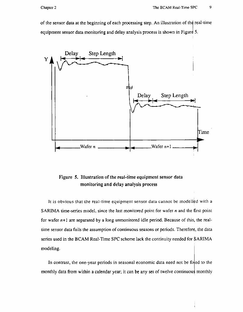
of the sensor data at the beginning of each processing step. An illustration of th
equipment sensor data monitoring and delay analysis process is shown in Figur
Time IF
CI Wafer n+l
Figure 5. Illustration of the real-time equipment sensor data monitoring and delay analysis process
It is obvious tha t the real-time equipment sensor data cannot be modelled with a
SARIMA time-series model, since the last monitored point for wafer n and the first point
for wafer n+l are separated by a long unmonitored idle period. Because of this, the real-
time sensor data fails the assumption of continuous seasons or periods. Therefore, the data
series used in the BCAM Real-Time SPC scheme lack the continuity needed for 6ARIMA
modeling.
In contrast, the one-year periods in seasonal economic data need not be fi
monthly data from within a calendar year; it can be any set of twelve

data points regardless of whether all twelve points fall within one particular calendar
Furthermore, the points in an economic data series tend to be continuous through ti
Therefore, although it may be ideal to use SARIMA time-series models for forecasting
economic data, it must be modified for application to the BCAM Real-lime SPC mod
See Figure 6 for a comparison of a continuous economic time-series data and
concatenated non-continuous equipment sensor time-series data.
Continuous Seasonal Economic Data
uu Season Season uu
Season Season
y x .
ne.
de.
a
Non-Continuous Periodic Equipment Sensor Data Y 103
13.40
13.20
13.00
12.80
12.60
12.40
12.20
12.00
0.00 50.00 100.00 150.00 200.00 250.00
1111 Period Period
Figure 6. A continuous economic time-series data vs. a non-continuous equipment sensor time-series data [2].

Chapter 2 The BCAM Real-Time SPC 11
In addition, the modified time-series models must be generated autom all ically for
practical use in the BCAM Real-Time SPC. This is because in a production enqironment,
a variety of products are run through each piece of equipment in any given lime. This
change in product lines might result in shifts and changes in the machine senso readings,
thus requiring that new models be generated in between runs. Furthermore, e current
method of generating time-series models is time-consuming and requires specia ized skills
in time-series statistics, as the models are generated interactively using standar statistical
analysis tools. Thus a methodology for automating the model generation proce 1 s must be
sought. Such a methodology has been developed and is discussed in the next chrapter.

12 Automatic Time-Series Model Generation Chapt
Chapter 3 Automatic Time-Series Model Generatio:
3.1 Background
Linear models can be, and have been, used in order to “forecast” future readings (
time series as a function of past readings and past forecast errors. This method of us
linear models for time-series forecasting is illustrated in Figure 7, where observation u
forecasted based on past observation wt-i with a forecast error of at using a sim
autoregressive model.
Wt-i Wt
Figure 7. Illustration of time-series modeling.
This method of time-series forecasting applies only to “stationary” data series
stationary time series has a mean, variance, and autocorrelation “structure” that
essentially constant through time. (The autocorrelation function, which is a wa)
measuring how the observations within a single data series are related to each other,
be used to determine the autocorrelation structure of a time series.) Non-statior
sequences are often differenced in order to achieve approximate stationarity.
3
a
’g
is
le
A
re
3f
ill
‘Y

Chapter 3 Automatic Time-Series Model Generation 13
3.2 Stationarity and Time-Series Integration
ARMA modeling applies only for a stationary time series. By definition,
An Autoregressive Integrated Moving Average (ARIMA) model is a algebraic
statement showing how a time-series variable (zJ is related to its own past vades ( q - 1 , zf-
1
a series is
2, ~ ~ - 3 , ...), i.e. autoregression, and its past forecast errors (af - ] , af-2, a,-3, ...), Le. moving
average [2]: I
P 9
i = 1 j = O
where w, = Vdz,
Vd : dth order of differencing
where V 1 z l = Z , - Z ~ - ~ , V ~ Z ~ = V ( V z , ) , ...
This is the form of the ARIMA model that is used for Real-Time SPC.
One typically generates ARIMA time-series models interactively by first identifying
appropriate models, estimating the model parameters, and checking the models for
adequacy. This is time-consuming and requires significant skills in using standard
statistical tools.
The ARIMA model generation process can be automated if the “integration”,
“autoregression” and “moving average” components can be separated and solved for
separately. This is typically done by first determining the differencing order necessary to
ensure that the data series is stationary, then determining the autoregressive order and
parameters using what is known as the modijied Yule-Walker equations, And finally
applying some appropriate technique to find the moving average order and parameters.

Chapu 14 Automatic Time-Series Model Generation
the data series is not stationary, its statistics, and perhaps its mean will shift through tir
Therefore, it would be expected that the estimated ACF for this series will drop slok
toward zero.
In order to determine whether a time series is stationary and if differencing
necessary, one looks at the estimated autocorrelation functions (ACFs) of the time se i
An autocorrelation function, again, is a way of measuring how the observations withi
single data series are related as a function of the time elapsed between the readings. 1
autocorrelation function at lag k is defined as follows [2]:
n - k
z tz t + k t = 1 n rk =
I = 1
- where Z1 = zl- z
and n = data count
. 3
e.
1Y
is
:S.
a
ie
2)
I
I
Chapter 3 Automatic Time-Series Model Generation 15
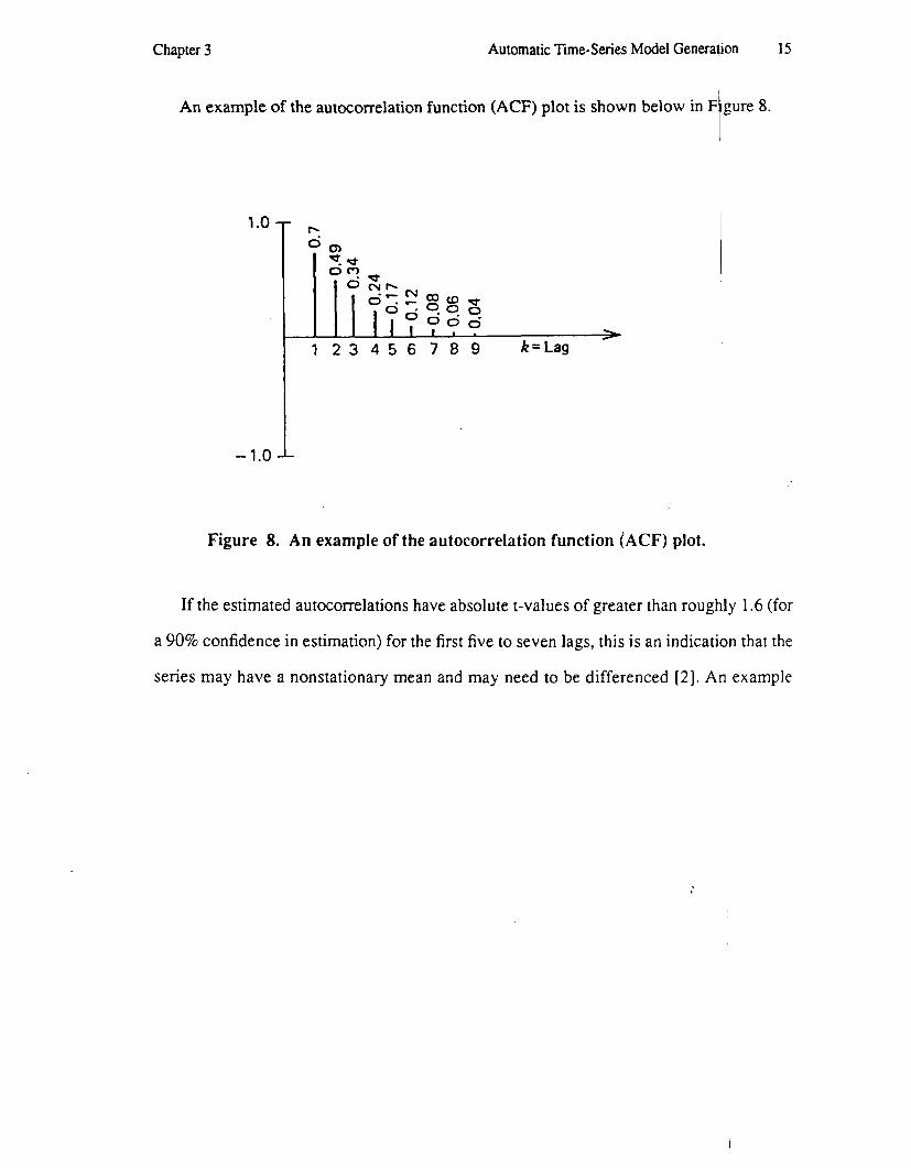
An example of the autocorrelation function (ACF) plot is shown below in F gure 8. I 1 .o
-1.0 I-
Figure 8. An example of the autocorrelation function (ACF) plot.
If the estimated autocorrelations have absolute t-values of greater than roughly 1.6 (for
a 90% confidence in estimation) for the first five to seven lags, this is an indication that the
series may have a nonstationary mean and may need to be differenced [2]. An example

16 Automatic Time-Series Model Generation Chap1
comparing the ACF plot of a stationary series and that of a nonstationary series is shc
in Figure 9.
Stationary Series mt.
Y
I I I
rmm
IO152
ioim
I0330
im m
95%
99.m
9830
9am
*-- 0 0.933191 I -0.020110 2 -0.0015742 J -0.011763
5 -0.093036 6 -0.066151 7 -0.029761 I 0.064555 Y -0 .047531
1 0 -0.070215 11 -0.0079384 U 0 . 1 3 4 9 9 1 13 -0.050692 I4 0.050967 15 0.0076100 1 6 -0 .013141
4 -0.oa0386
17 -0.ao9ios
ao 0.051425
11 -0.0029126 1 9 -0.014250
DrTal.IiIP 1.00000
-0.01237 - 0 . O O Y 1 Y -0 .092#7 -0 .Ol 115 - 0 . 09970 -0.07019 -0.03119 0.06931
4 . 0 5 0 9 4 -0.07515 -0.00151
0 .14465 -0.05132
O . O Y S 2 O.OOll5 -0.08910 4 . 1 1 7 6 7 -0.003Lz -0.OlS17
O . O U 6 1
Nonstationary Series Dum
Y
trim
109 m
101m
lam mm
IlMO
lam
106.03
Irn.03
lozaD
lOl.03
iwm mm urn
x ooo m m Dpm Pam a m
*-- 0 5.414706 1 1.14Y605 2 *.I27795 3 3.I30654 4 3.43599) 5 3.099Sl9 6 2.110195 7 2.747171 8 1.641275
1 0 2.J41620 I1 1.306211
9 a.412554
II a.at3695 13 a . u i 1 0 3 I4 2.001750 15 1.797123 1 6 1.557179 17 1.422054 I 1 1.3Y4061 1 9 l .JW111 1 0 1.J47006
-.elm 1.00000 -1 I 9 1 7 6
0.I9564 0.7V927 I 1
0.70745 I 0.63457 I 0.17244 I 0.51194 I 0.50736 I 0.41791 I 0.45141 0.43375 I I
0.42591 I 0.&2176 I 0.3Y177 I 0 . 3 0 6 9 I 0.33203 I
0.26071 I 0.2S716 1 0.25110 1 0.24177 I
o . a t x o I
-.- u u
' :.?.?2.!.:.!2.! I................ I................ ............... .............. I........... I........... I.......... I...'.'..'. .......... .......... 1.. ....... 8 ........ 1 ........ I ....... I ....... ....... ....... ....... ....... I..... . - .c- m.
Figure 9. Comparison of the ACF plots of stationary and nonstationary data.
In order to determine the estimated t-values and test the significance of
autocorrelation coefficients, one must first estimate the standard error of the ACFs. N
Barlett [5 ] has derived an approximate expression for the standard error of the sampl
distribution of the autoregressive coefficient rk. This estimated standard error, designa
s(rk), is calculated as follows:
* 3
In
X
1 * I I I I
I I I I I 1 I I I I I I I I I l
le
s.
'g
:d
Chapter 3 Automatic Time-Series Model Generation 17
This expression is appropriate for processes with normally distributed ran om shocks
Now one can use the estimated standard errors to test the null hypothesis 0: pk = 0
for k = 1,2,3, .... This hypothesis is tested by finding out how far away the samble statistic
rk is from the hypothesized value pk = 0. This distance is expressed as a r-statisfic equal to
the equivalent number of estimated standard errors. Thus one can approxibate the t-
statistic in the following fashion [Z]:
! where the true MA order of the process is k- 1.
I
3.3 The Yule-Walker Equations and A R Modeling
The Yule-Walker equations are used for determining the AR model for a known AR
process. These equations describe the linear relationship between the AR parameters and
the autocorrelation function. The solution of these equations is provided by the
computationally efficient Levinson-Durbin algorithm [6].
A relationship between the AR parameters and the autocovariance functiod R,, of w,
is presented. This relationship is known as the Yule-Walker equation [7]. The ddrivation of
the Yule-Walker equation proceeds as follows [6 ] : i

18 Automatic ‘Iime-Series Model Generation
where wt is the observation from a stationary time series, at is the forecast error or nc
and E[] implies the expected value.
We will define the following:
But R d k ) = 0 for k > 0 since a future input to a causal, stable filter cannot affeci
present output and a, is “white” noise. In other words, since a, is a white excitation,
uncorrelated with those wz occurring prior to t. Therefore, Expression ( 5 ) can be fur
simplified as:
i = 1
Expression (7) is known as the Yule-Walker equations. To determine the
parameters, one need only choose the first p equations from Expression (7) for k > 0, SI
for 49, ..., $& and then find c? from Expression (7) for k = 0. The set of q u a t
which require the fewest lags of the autocovariance function is the selection k = 1,2, ..
They can be expressed in matrix form as [6]:
:r 3
(5)
se,
(6)
;he
. is
ier
[7 1
iR
ve
Ins
P-

Chapter 3 Automatic Time-Series Model Generanion 19
It should be noted that Expression (8) can also be augmented to incorporate the o2
equation, yielding
which follows from Expression (7).
The Levinson-Durbin algorithm provides an efficient solution for Expressiob (9). The
algorithm proceeds recursively to compute the parameter set ($1 1, ( 5 1 ), ($21, $22,(52 1, ...,
QP2, ..., $pp, op2). Note that an additional subscript, p , has been added to the AR
coefficients to denote the order of each sequence. The final set at order p is the desired
solution [6] . In particular, the recursive algorithm is initialized by setting:
2 2

20 Automatic Tune-Series Model Generation Chapkr 3
1 ,2 , . . . , p and hence $pl,p+l = 0. In general for an AR orderp process, +fi = 0 and q2
0: for k > p . Hence, the variance of the excitation noise is a constant for a model
equal to or greater than the correct order. Thus, in theory, the point at which o k 2 does
change would appear to be a good indicator of the correct model order. This means
02 first reaches its minimum at the correct model order [6] .
with the recursion for i = 2.3, ..., p given by
=
order
;lot
tiat
k- I
- i = l +kk - 2
O k - 1
- @kj - @IC- 1, j -k @kk@k- 1, k- j
It is important to note that (Qkl , Qk2, ..., OM, q2), as obtained above, is the Sam{ as
would be obtained by using Expression (9) for p = k. Thus the Levinson-Durbin a l g o r i b
also provides the AR parameters for all the lower order AR model fits to the data. This
useful property when one does not know u priori the correct model order, since one
use Expression (9) to generate successively higher order models until the modeling ehor
ak2 is reduced to the desired value. ~
1
3.4 The Modified Yule-Walker Equations and ARMA Modeling I
The Yule-Walker equations can be modified in order to generate ARMA models.
illustrate this, let wy be a stationary time series generated by the following AR A p.s equation:

Chapter 3 Automatic Time-Series Model Generation 21
P 9
Multiplying both sides of Equation (15) by Wt-k and taking the expect tions, we b obtain: I
P 9
Rxx (k) = QiRXx (k - i ) + 0 .RnX 1 (k - j ) (16) i = l J = o
where, once again, !
However, as pointed out in Section 3.2.3, one can assume that R,,(k) = 0 for k > 0.
Therefore,
P q
$RXx (k - i ) + 1 ejR,, (k - j ) , i = 0, ..., q
Q i R X x ( k - i) , i = q + 1, q + 2, . . .
(19) i = l j = O
P
i = l
Thus the AR parameters can be estimated independently of the MA param
uses the Yule-Walker equations as given by Expression (19) (81.
A popular approach for determining the ARMA model and estimating its paxtameters is
to use i > 4 to find the AR parameters (Q1, 49, ..., Q p ) and then apply some a propriate P

22 Automatic Time-Series Model Generation Chap
technique to find the MA parameters (el, 02, ..., €I4) or an equivalent parameter set.
example, to find the AR parameters, using Expression (19) and i = q+l , q+2, ..., q+p.
solve the following matrix expression:
P X X I
These equations have been called the extended, or modified, Yule-Walker equations.
The AR order can be determined by testing the singularity of the correlation ma
1R.J. Therefore, in order to choose an appropriate model order p for the AR portion of
ARMA model, the property
detlRx,I = 0
for dimension of lRxxl greater than the AR order p can be used. The AR coefficients
49, ..., $,J can then be solved using the linear system of equations in Expression (20).
Expression (19) can be used to determine the MA order 4, since q is seen to be
largest integer k for which
:r 3
- ‘or
we
!O)
r i X
:he
!l)
P l y
he
’2)

Chapter 3 Automatic Time-Series Model Generalion 23
This process can be repeated with the new estimate of the MA order q.
MA coefficients (91, 92, ..., 04) can be determined using appropriate
techniques [ 81.
3.5 Modifications to Time-Series Model Generation Algorithm for Noise Compensation
An inherent problem with automatic time-series model generation for the B c A M SPC
scheme is that the real-time sensor signals tend to be very noisy. This mahes it very
difficult to determine the AR order using the matrix form of the modified YuUe-Walker
equations:
where
for dimension of lRxxl greater than the AR order p . This is because it is very difficult to
test whether the determinant of the correlation mamx IRJ has reached zero.
However, Expression (19) can be used to determine the AR order as well as the AR
coefficients (ql, Q2, ..., qP) using simple linear regression. Expression (19) is rep
for convenience:
24 Automatic Time-Series Model Generation Chap1
P q
x @ i R x x ( k - i ) + x e , R , , ( k - j ) , i = O , . . . , q
C $ i ~ x x (k- i ) , i = q + I , q + 2, ... j = O (
i = 1
P
i = l
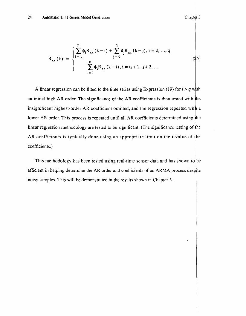
A linear regression can be fitted to the time series using Expression (19) for i > q v
an initial high AR order, The significance of the AR coefficients is then tested with
insignificant highest-order AR coefficient omitted, and the regression repeated wit
lower AR order. This process is repeated until all AR coefficients determined using
linear regression methodology are tested to be significant. (The significance testing of
AR coefficients is typically done using an appropriate limit on the t-value of
coefficients .)
This methodology has been tested using real-time sensor data and has shown tc
efficient in helping determine the AR order and coefficients of an ARMA process des:
noisy samples. This will be demonstrated in the results shown in Chapter 5.
. 3
5 )
th
le
a
ie
ie
le
se
te

Chapter 3 Automatic Time-Series Model Generation 25
3.6 Summary
The process of automatically generating ARIMA time-series models essentially boils
down to determining an optimal model order structure as represented by a point in a three-
dimensional space as shown in Figure 10.
I ,
‘ MA order q
Differencing order d
Figure 10. Algorithm for determining the structure of an ARIMA model.
The model generation process starts by determining the appropriate differenicing order
needed in order to derive a “stationary” time series, thus reducing the problem down to a
search for an optimal point i n a two-dimensional space. The modified Yule-Walker
equations are then used with a high initial guess for the MA order 9 in order toldetermine
the AR order p and the AR coefficients (@ly @2? ..., @p). The same modified Yule-Walker
equations can then be used to estimate the MA order q as shown using ExpreJsion (22).
This process is then repeated with the new estimate of the MA order q until the process
converges. The MA coefficients (el7 0zY ...) eq) are then solved using iterative optimization
techniques.

26 Modified Real-Time SPC with Automatic Xme-Series Model Generation Cha]
Chapter 4 Modified Real-Time SPC with Automat Time-Series Model Generation
4.1 Overview of Modifications
As explained in section 2.2, one cannot use the seasonal ARIMA (SARIMA) mod
order to model equipment sensor data for real-time SPC purposes. However, one
modify the method in which ARIMA models are generated in order to devi
satisfactory filters for real-time SPC. This is done by decomposing the original se
signal into two components, the within-wafer and wafer-to-wufer components, an
developing two separate ARIMA models: one for modeling the characteristics of the
variation from within the critical step of each wafer and one for modeling the wafe
wafer variation of the real-time sensor data. These models can be generated automatii
using the algorithm described in Chapter 3.
The within-wafer and wafer-to-wafer residuals can then be combined into two sep;
T2 statistics for SPC purposes. One will be used for detecting within-wafer proces
:r 4
3 I
I in
:an
OP
sor
by
ata
to-
1lly
ate
ing

Chapter 4 Modified Real-Time SPC with Automatic lime-Series Model Generation 27
faults while the other will be used for detecting wafer-to-wafer faults. An exarfpple of the
signal decomposition and filtering process is shown in Figure 11.
Sensor Signal Decomposition Filtered Reslduals
I I I I I U Y Y U Y
Figure 11. Example of the signal decomposition and filtering process.
4.2 Within-Wafer Data Modeling and Filtering
After carefully analyzing the equipment sensor data, it can be seen that the sensor data
display a distinctive auto-correlated pattern during each wafer processing step. This
pattern tends to repeat itself with every wafer processed. An ARIh44 model can
order to model the characteristics of these within-wafer patterns by selectively
only the time-series autoconelations within each wafer. The within-wafer

28 Modified Real-Time SPC with Automatic Time-Series Model Generation
'g
1s
e
x
Chapte
1m
1 3
1m
050
am
-ow
models and filtered residuals can be used to detect slight problems in the wafer processi
step. Shown in Figure 12 is an example of this repeated pattern for select sensor sign;
from the Lam Research Rainbow plasma etcher and the IIND residuals after filtering t
data with the automatically generated ARIMA time-series models.
'
I ! i
I ! ! .I 1 . . - _ _ . . . i . - I
- 1 i I I I
De-meaned Sensor Data
I I I
Impedance - lk-wcurcd Y l l d
060
040 020 om Q 10
440
4)(0
480 - 1 m - 1 20
.I a
ylm im m 1x8 m 2mm 003
Phase - Demeaned Y, Id
Within-Wafer Residuals
Phase - Residuals Y X I ~
3m 25.3
2m 1 5 0
1m Ox) Om
.om
.I 00
.I 50
Figure 12. Selected equipment sensor data from the Lam Research Rainbow plasma etcher showing the repeated auto- correlated pattern for each wafer processed and their corresponding IIND residuals after filtering. Sensor data for each wafer have been de-meaned so that the within- wafer time-series pattern can be seen more easily.
Modifications to the ARIMA model generation algorithm must be made in order
generate an appropriate model for the de-meaned within-wafer data. The modificatio
simply involve calculating the time-series statistics (i.e. the autocorrelation
using selective samples that embody only the within-wafer time-series

chapter 4 Modified Real-Tie SPC with Automatic Tme-Series Model Genenation 29
This means eliminating samples involving uncorrelated datapoints across /wafers. An
illustration of this selective sampling process is shown in Figure 13. !
Correlated Sample
Figure 13. An illustration of the selective sampling process for determining within-wafer ARIMA time-series models.
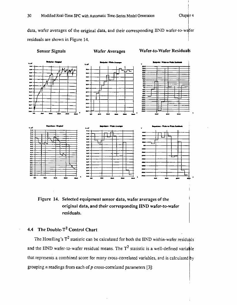
4.3 Wafer-to-Wafer Data Modeling and Filtering
Although most sensor data show little autocorrelation across wafers, therei are certain
signals that have significant autocorrelation from wafer to wafer. This wafkr-to-wafer
correlation must be filtered with an appropriate time-series model. By looking at only the
correlations between the wafer averages, one can build time-series models that will be
able to filter these wafer-to-wafer correlations. The wafer-to-wafer time-series odels and
filtered residuals can be used to detect catastrophic problems in the wafer pr J essing step
(i.e. a significant shift in the real-time sensor signal). Selected original equiprjlent sensor
30 Modified Real-Time SPC with Automatic Time-Series Model Generation
)le
by
Chapt
data, wafer averages of the original data, and their corresponding IIND wafer-to-wa
residuals are shown in Figure 14.
Sensor Signals
--- 1.3
I
Wafer Averages
-.-A- v .3
Wafer-to-Wafer Residual
Qp
a- 1Do u
I f r- I l l l I I I I 1 I I
I I
I I I Y Y Y
- I U I
Figure 14. Selected equipment sensor data, wafer averages of the original data, and their corresponding IIND wafer-to-wafer residuals.
4.4 The Double-T2 Control Chart
The Hotelling's T2 statistic can be calculated for both the IIND within-wafer residL
and the IIND wafer-to-wafer residual means. The T2 statistic is a well-defined varia
that represents a combined score for many cross-correlated variables, and is calculated
grouping n readings from each of p cross-correlated parameters [3]:

Chapter 4 Modified Real-Time SPC with Automatic Time-Series Model GeneraWion 3 1
T ~ = ~ ( X - X ) = s -1 ( X - X )
where group mean XT = [XI.. .Xp]
nominal value XT = [ i , . . . ~ ~ ]
s1 2 ... Slp
variance-covariance matrix s = 1 i .., i 1 The distribution of the T2 statistic is related to the F-distribution as follows:'
The T2 statistic defined above is optimal for detecting mean shifts nder the
assumption of multivariate normality. Furthermore, it can be extended to guaird against
shifts in the variance of the monitored data. However, it is not geared towards identifying
a shift in the variance-covariance matrix and will confound such a shift with a Shift in the
mean vector.
i.
This statistic takes a low value when the average values of the cross-@orrelated
variables are small. The T2 score is very sensitive to any change in the mean of one or
more of the combined variables. This score can be used in conjunction with a one-sided
control chart whose limit is determined according to the number of variables, tlhe sample
As noted above and in Expression (26), readings are grouped according to I specified
(or group) size and the acceptable percentage of false a l m s .
group size n and a T2 statistic is calculated for each group. This grouping is n
noisy spike in the data will not cause a large T2 alarm given that the fault is
order to compensate for the occasional noise in the real-time data. Thus an

32 Modified Real-Time SPC with Automatic Time-Series Model Generation Chap
The Double-T2 Control Chart is a one-sided control chart displaying both the wit
wafer and the wafer-to-wafer T2 statistics in order to determine if a process is in a stat
control. If a process goes out of control, one can determine whether the alarm was cai
by a within-wafer or wafer-to-wafer fault. An example of the Double-T2 Control Cha
shown in Figure 15.
20.6
t2.m
8.W
F gure 15. An example of a Double-T2 Control Chart. The line graph plots the within-wafer T2 statistic with a specified group size. The bar graph shows the wafer-to-wafer T2 statistic
for each wafer processed. (NOTE: The two T2 statistics have been scaled so as to have the same control limit.)
3
4.5 Summary
In conclusion, an automatic ARIMA time-series model generator has been adde,
the BCAM Real-Time SPC module in order to make the application more practical
robust. Furthermore, the system has been modified so that two time-series models
generated for each signal in order to filter the within-wafer and wafer-to-wafer varia
:r 4
in-
of
ced
t is
to
.nd
3re
Ion

Chapter 4 Modified Real-Time SPC with Automatic ‘lime-Series Model Generation 33
separately. This in terms implies the generation of two separate T2 statistics f4r real-time
SPC: one for signalling within-wafer faults and the other for signalling wafer-to-wafer
faults. These two T2 statistics are scaled and plotted together on what is called a Double-
T2 Control Chart. This scheme has been implemented in software and harddare, and is
discussed in the following chapter. !
34 Implementation and Experimental Results Chap
Chapter 5 Implementation a,id Er perimental Resul
5.1 Implementation
5.1.1 The BCAM Real-Time SPC System
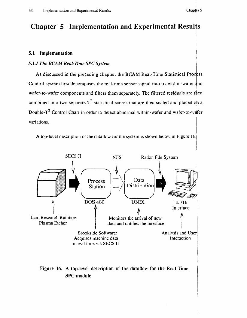
As discussed in the preceding chapter, the BCAM Real-Time Statistical Pro(
Control system first decomposes the real-time sensor signal into its within-wafer
wafer-to-wafer components and filters them separately. The filtered residuals are t
combined into two separate T2 statistical scores that are then scaled and placed (
Double-T2 Control Chart in order to detect abnormal within-wafer and wafer-to-w
variations.
A top-level description of the dataflow for the system is shown below in Figure 16
SECS I1 NFS Radon File System
DOS 486 UNIX Tcl/Tk Interface 4
Monitors the anival of new data and notifies the interface
t Lam Research Rainbow
Plasma Etcher
Brookside Software: Acquires machine data
in real time via SECS I1
Analysis and Use Interaction
:r 5
S
ss
Id
:n
a
er
Figure 16. A top-level description of the dataflow for the Real-Time SPC module
Chapter 5 Implementation and Experimental Results 35
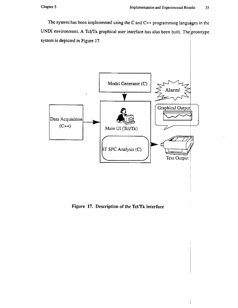
The system has been implemented using the C and C++ programming langu
UNIX environment. A T c u k graphical user interface has also been built.
system is depicted in Figure 17.
Data Acquisition
Model Generator (C) I le Main UI (Tclnk)
Graphical Outpu I= Text Output
Figure 17. Description of the Tcl/Tk interface

36 Implementation and Experimental Results Chap!
A screen dump of the Real-Time SPC graphical user interface is shown in Figure
This interface includes a main panel, a model generation panel, and a Real-Time S
window.
-4A1-n h T u s a n I i m O 5 . M
Figure 18. Real-Time SPC screen dump
r5
8.
'C
Chapter 5 Implementation and Experimental Results 37
Time-Series Original Sensor Model Data Generation
Algorithm -m
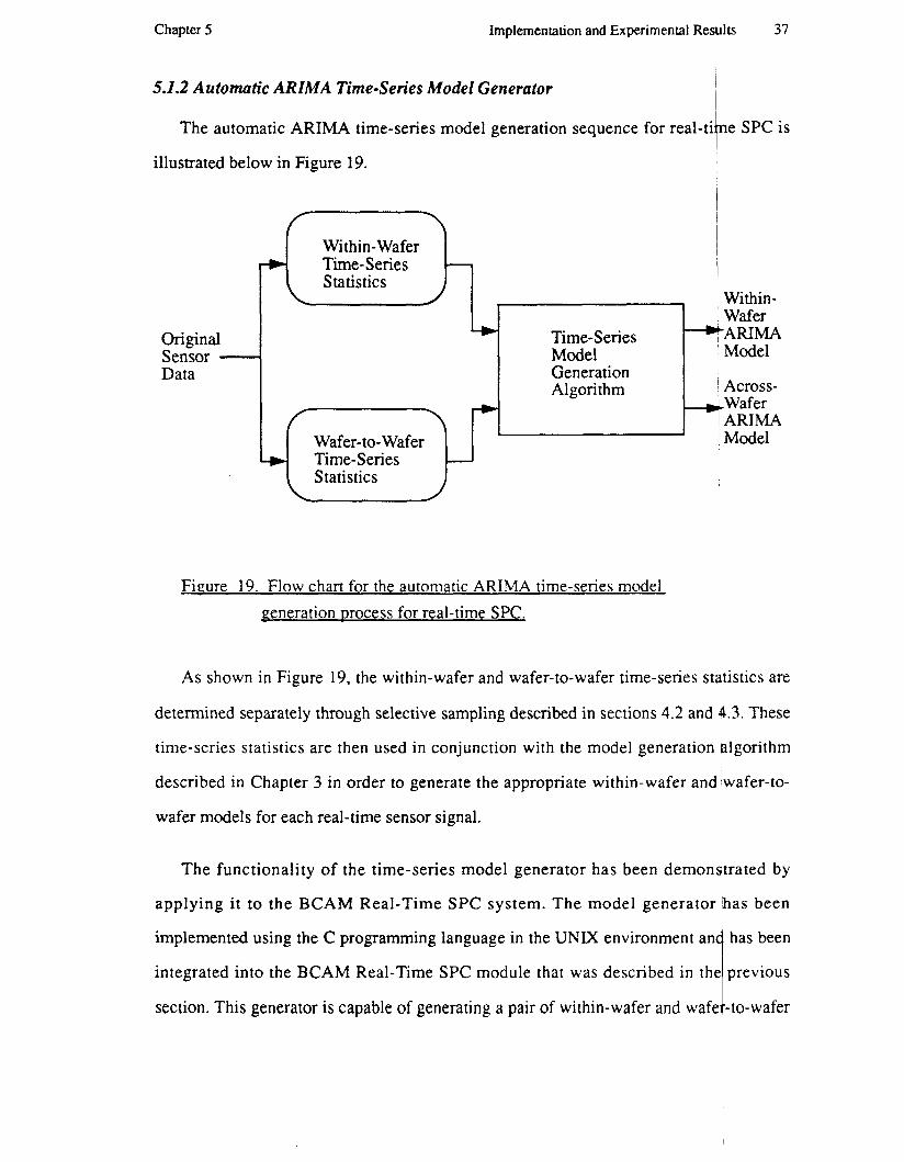
The automatic ARIMA time-series model generation sequence for real-ti
5.1.2 Automatic ARIMA Time-Series Model Generator
illustrated below in Figure 19.
Wafer -ARIMA
Model
1 Across- Wafer AFUMA
Wafer-to- Wafer
Figure 19. Flow chan for the automatic ARIMA time-series model generation Drocess for real-time SPC.
Model
As shown in Figure 19, the within-wafer and wafer-to-wafer time-series statistics are
determined separately through selective sampling described in sections 4.2 and 4.3. These
time-series statistics are then used in conjunction with the model generation ralgorithm
described in Chapter 3 in order to generate the appropriate within-wafer and <wafer-to-
wafer models for each real-time sensor signal.
Time-Series
The functionality of the time-series model generator has been demonsitrated by
applying i t to the BCAM Real-Time SPC system. The model generator has been
implemented using the C programming language in the UNIX environment an
integrated into the BCAM Real-Time SPC module that was described in
section. This generator is capable of generating a pair of within-wafer and
7

38 Implementation and Experimental ResulLs Chapljer 5
AFUMA models in less than five seconds real time and less than one second CPU tim on
a Sun SPARCstation 2m. J 5.2 Experimental Results
5.2.1 Summary of Experiment
The following experiment was demonstrated in the SRC Real-Time Statistical Pro(
Control Workshop at the University of California, Berkeley, on May 10-11, 1993
involves the generation of five pairs of within-wafer and wafer-to-wafer ARIMA ti1
series models for five signals. These signals were the Coil Position, the Impedance,
Phase Magnitude, the Tune Vane and the Peak-to-Peak Voltage collected from the L
Research Rainbow plasma etcher in the Berkeley Microfabrication Laboratory. Twe
polysilicon wafers were processed in order to produce the baseline data needed for
5 s
It
ie-
he
Im
ve
he

Chapter 5 Implementation and Experimental Results 39
generation of the time-series models. The signals, along with their correspond
wafer and wafer-to-wafer filtered residuals are shown below in Figure 20.
ng within-
Baseline Data
4- 1 ................................... *- . u tm .*I
Within-Wafer Residuals
I !
u riu
Wafer-to-WAfer Residuals,
Figure 20. Baseline data for five sensor signals along with their corresponding wit hin-wafer and wafer-to-wafer filtered residuals.

40 Implementation and Experimental Results Chapt
Signal
Coil
Impedance
The within-wafer and wafer-to-wafer ARIMA time-series models generated using
automatic time-series model generator is shown in Table 1.
Within-Wafer Model Wafer-to-Wafer Model
ARIMA(2,0,1) ARIMA(2,0,1)
ARIMA(2,1,0) ARIMA( 1 , 1 ,O)
Table 1: Within-Wafer and Wafer-to-Wafer ARIMA Models Used for Experimei
Phase
Tune
~~
AMMA( 1 ,O,O) ARIMA( 1,0,2)
ARIMA( 1 ,O,O) ARIMA(O,l,O)
Volt ARIMA(O,O,O) ARIMA(l,O,l)
After the appropriate baseline models have been built, fourteen wafers were proces
and monitored using the BCAM Real-Time SPC scheme through the Tcl/Tk interf
described in Chapter 5. Known faults were introduced as follows in Table 2:
Wafer #
1-7
8-9
10
I1
12-14
Table 2: Description of Wafers in Real-Time SPC Experiment
Description
Clean wafers with blanket polysilicon layer
Wafers with dirty polysilicon film
Clean wafer with blanket polysilicon layer
Wafer from wrong batch with photoresist remaining
Clean wafers with blanket polysilicon layer
:r 5
:he
It
led
ice

Chapter 5 Implementation and Experimental Results
Figure 21. Original Sensor signals and their corresponding within- wafer residuals with a 3-0 control limit.
41
5.2.2 Within- Wafer Residuals
The original sensor signals and their corresponding within-wafer residuals e shown I.. in Figure 2 1.
I Sensor Signal Within- Wafer Residuals
42 Implementation and Experimental Results Chap
One can see significant within-wafer problems in wafers #9 and #11. This is obvi
because wafer ##9 was deposited with dirty polysilicon film and wafer #11 came from
wrong batch and contains unwanted photoresist. One can also see slight within-w,
problems with wafers #3, #6, #8 and #lo. (This is most obvious by looking at the orig
signals and residuals of the Tune Vane, the Phase Magnitude and the Impedance.) W
#8, like wafer #9, was also deposited with dirty polysilicon film. Wafers #3, #6 and
did not have any known problems.
Wafers #8, #9 and #11 are known to be faulty wafers and are correctly identified by
within-wafer residuals. Wafers #3, #6 and #10 might possess prob!ems that were unknc
prior to the runs.
r 5
us
he
er
la1
.er
10
he
vn
Chapter 5 Implementation and Experimental Results 43
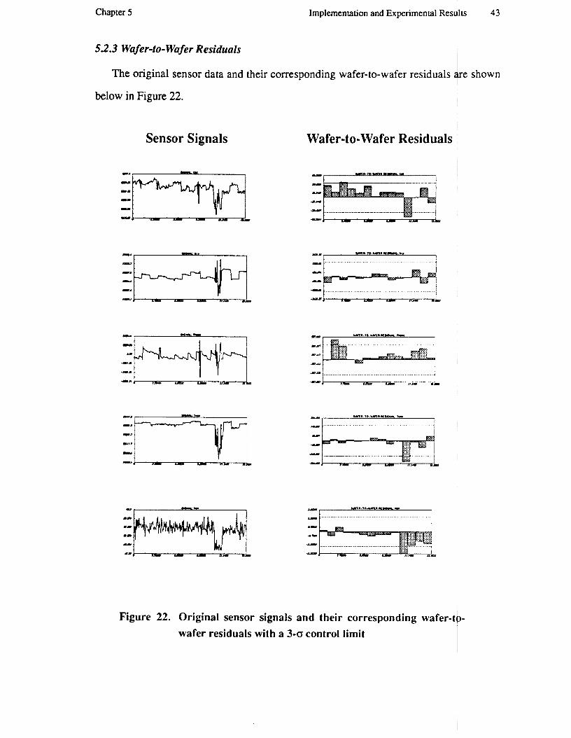
52.3 Wafer-to-Wafer Residuals I
The original sensor data and their corresponding wafer-to-wafer residuals e shown + below in Figure 22. I
Sensor Signals
Y
u
411
Wafer-to-Wafer Residuals
I UT..,..-. JN Q I
............................................................ I - -- I Lpit u ,,- IFh,
-py- wm .:I. ............. ..... :.:.: :+y. .:.:.:.: ..A. C
-my
............................................................ -- ' i II llD. w 11- II- -n.o
Figure 22. Original sensor signals and their corresponding wafer-t wafer residuals with a 3-0 control limit

44 Implementation and Experimental Results
The wafer-to-wafer residuals tend to detect catastrophic faults, since a large wafer-
wafer residual usually signifies a major mean shift in the sensor signal. It is therefore
obvious by looking at the original signals and the wafer-to-wafer residuals that there
significant problems with wafer #11. This is easily seen by looking at the mean shifts
the Tune Vane, the Peak-to-Peak Voltage, and the Coil Position. The mean shifts in
signals are also reflected in their respective wafer-to-wafer residuals. Thus by looking
the wafer-to-wafer residuals, one can detect a significant problem with wafer #11, which
I ~
Chap* 5
to-
are
in
thsse
at
The within-wafer and wafer-to-wafer T2 statistics are plotted on the Double-T2
Control Chart shown below in Figure 23.
20.12
i2.m
8.W
4 . m
0
Figure 23. Double-T2 Control Chart from the experiment. (NOTE: The line plots are the within-wafer T2s and the bar plots are the wafer-to-wafer T’s.)
One can see that the within-wafer T2 statistics were able to signal problems I i t h
wafers #3, #6, #8, #9, #10 and #11, with numerous significant T2 alarms for wafers #9 nd

Chapter 5 Implementation and Experimental Results 45
wafers, which were unknown prior to the run.
The wafer-to-wafer T2 statistics clearly identified the catastrophic fault in
which is a wafer with unwanted photoresist. Since this was the only wafer
significant mean shifts in the sensor signals, it was the only one with an wafer-to-wafer
alarm generated.
wafer #11,
:hat cause
T2
The experiment shows that the automatic time-series model generator d a s able to
generate satisfactory models for detecting wafer or processing faults in teal-time.
Furthermore, the modified real-time SPC scheme is shown to be effective in detecting two
different types of faults: slight faults caused by within-wafer processing instauilities and
catastrophic faults resulting from major mean shifts in the sensor signals.

46 Conclusions and Future Work Chapt
Chapter 6 Conclusions and Future Work
The BCAM Real-Time Statistical Process Control scheme has been modified, and
automatic time-series model generator has been developed and integrated in the BCl
SPC module. This modified scheme along with the automatic model generation algorit
has been applied on the Lam Research Rainbow single-wafer plasma etcher. The mo
generation algorithm has demonstrated success in generating useful time-series models
filtering real-time sensor data. Furthermore, the modified real-time SPC scheme has bc
shown to be superior in detecting processing faults than the originally propoi
methodology.
The modifications made to the BCAM Real-Time SPC scheme involve decompos
the original sensor signals into two separate components to be analyzed independently:
within-wafer and wafer-to-wafer time-series components. Separate T 2 statistics for
within-wafer and wafer-to-wafer analyses are then plotted on a Double-T2 Control Ch
This will allow one to not just detect processing faults, but also determine whether th
faults are minor problems resulting from within-wafer processing instabilities,
catastrophic processing errors resulting from major mean shifts in the equipment sen
signals.
The automatic ARIMA time-series model generation algorithm involves determin
the Integration, Autoregressive and Moving Average components of the model separatc
This algorithm is facilitated by the use of the modified Yule-Walker equations [
Furthermore, this algorithm has been modified so that the original equipment sen
signals may be decomposed and separate models generated for the within-wafer i
wafer-to-wafer time-series data.
r 6
m
M
m
el
or
:n
:d
'g
he
ne
rt.
se
or
or
'g
lY.
i] .
or
id

Chapter 6 Conclusions and Future Wbrk 47
The automatic time-series model generation algorithm has the potential f making
several other computer-aided manufacturing applications more practical and ro ,G ust. These
applications include equipment modeling, real-time equipment control, wafek-to-wafer
control and real-time equipment diagnosis. Further studies will be conducted In order to
determine the feasibility of applying time-series modeling to the CAM applications
mentioned above.
In addition, other methods for filtering the sensor data for real-time SPC will be
studied. These include possible use of the Kalman Filters, the theory of principle
components or just simple exponentially-weighted moving averages.


References
[ 13 Douglas C. Montgomery, Introduction to Statistical Quality Control, 2nd edition,
New York: John Wiley & Sons, 199 1.
[2] Alan Pankratz, Forecasting with Univariate Box-Jenkins Models - Concepts and
Cases, New York: John Wiley & Sons, 1983.
[3] Richard J. Harris, A Primer ofMultiuariate Statistics, London: Academic h s s , 1975.
[4] Costas J. Spanos, Hai-Fang Guo, Alan Miller and Joanne Levine-Panill, “Real-Time
Statistical Process Control Using Tool Data”, IEEE Transactions on Semiconductor
Manufacturing, Vo1.5, No. 4, pp. 308-31 8, November 1992.
[5] M.S. Bartlett, “On the Theoretical Specification of Sampling Propemes of Autocorre-
lated Time Series”, Journal of the Royal Statistical Society, Vol. B8, p. 27, 1946.
[6] Steven M. Kay and Stanley Lawrence Marple, Jr., “Spectrum Analysis - A Modern
Perspective”, Proceedings of rhe IEEE, Vol. 69, No. 1 1, pp. 1380- 14 19, November
1981.
[7] G.E.P. Box and G.M. Jenkins, Time Series Analysis: Forecasting and Control, San
Francisco: Holden-Day, 1976.
[8] Joseph C. Chow, “On Estimating the Orders of an Autoregressive Moving-Average
Process with Uncertain Observations”, IEEE Transactions on Automatic Control, pp.
707-709, October 1972.