This is an electronic reprint of the original article.This reprint may differ from the original in pagination and typographic detail.

Powered by TCPDF (www.tcpdf.org)

This material is protected by copyright and other intellectual property rights, and duplication or sale of all or part of any of the repository collections is not permitted, except that material may be duplicated by you for your research use or educational purposes in electronic or print form. You must obtain permission for any other use. Electronic or print copies may not be offered, whether for sale or otherwise to anyone who is not an authorised user.

Buyukdagli, Sahin; Ala-Nissilä, Tapio

Electrostatic energy barriers from dielectric membranes upon approach oftranslocating DNA molecules

Published in:JOURNAL OF CHEMICAL PHYSICS

DOI:10.1063/1.4942177

Published: 28/02/2016

Document VersionPublisher's PDF, also known as Version of record

Please cite the original version:Buyukdagli, S., & Ala-Nissilä, T. (2016). Electrostatic energy barriers from dielectric membranes upon approachof translocating DNA molecules. JOURNAL OF CHEMICAL PHYSICS, 144(8), [084902]. DOI:10.1063/1.4942177

Electrostatic energy barriers from dielectric membranes upon approach oftranslocating DNA molecules

Sahin Buyukdagli, and T. Ala-Nissila,

Citation: The Journal of Chemical Physics 144, 084902 (2016); doi: 10.1063/1.4942177View online: http://dx.doi.org/10.1063/1.4942177View Table of Contents: http://aip.scitation.org/toc/jcp/144/8Published by the American Institute of Physics

THE JOURNAL OF CHEMICAL PHYSICS 144, 084902 (2016)

Electrostatic energy barriers from dielectric membranes upon approachof translocating DNA molecules

Sahin Buyukdagli1,a) and T. Ala-Nissila2,3,b)1Department of Physics, Bilkent University, Ankara 06800, Turkey2Department of Applied Physics and COMP Center of Excellence, Aalto University School of Science,P.O. Box 11000, Espoo, FI-00076 Aalto, Finland3Department of Physics, Brown University, P.O. Box 1843, Providence, Rhode Island 02912-1843, USA

(Received 17 November 2015; accepted 5 February 2016; published online 23 February 2016)

We probe the electrostatic cost associated with the approach phase of DNA translocation events.Within an analytical theory at the Debye-Hückel level, we calculate the electrostatic energy ofa rigid DNA molecule interacting with a dielectric membrane. For carbon or silicon based lowpermittivity neutral membranes, the DNA molecule experiences a repulsive energy barrier between10 kBT and 100 kBT . In the case of engineered membranes with high dielectric permittivities, themembrane surface attracts the DNA with an energy of the same magnitude. Both the repulsiveand attractive interactions result from image-charge effects and their magnitude survive even forthe thinnest graphene-based membranes of size d ≈ 6 Å. For weakly charged membranes, theelectrostatic energy is always attractive at large separation distances but switches to repulsive closeto the membrane surface. We also characterise the polymer length dependence of the interactionenergy. For specific values of the membrane charge density, low permittivity membranes repel shortpolymers but attract long polymers. Our results can be used to control the strong electrostatic energyof DNA-membrane interactions prior to translocation events by chemical engineering of the relevantsystem parameters. C 2016 AIP Publishing LLC. [http://dx.doi.org/10.1063/1.4942177]

I. INTRODUCTION

The DNA molecule plays a crucial role in mediatingbiological information during the assembly of the buildingblocks of living organisms. As the carrier of the geneticcode, DNA plays a central role in various biologicaland technological processes such as cell division,1 proteinbiosynthesis,2 drug delivery,3 and DNA profiling.4 Theefficient use of DNA in biological and nanotechnologicalapplications necessitates fast access to its genetic contentand an accurate knowledge of its interaction with thesurrounding medium. Considering the omnipresent couplingbetween strongly charged DNA molecules, the dielectric watersolvent embodying charges, and external macromoleculesand membranes in nature, a proper modelling of DNAelectrostatics is essential.

A fundamental question concerning DNA in biologicaland artificial systems concerns the electrostatic interactionsbetween fluctuating polymers and membranes. This has beenmainly considered at the mean-field (MF) Poisson-Boltzmann(PB) level. The electrostatic MF approximation has theadvantage of allowing the consideration of entropic polymerfluctuations. The corresponding formalism consists ofcoupling Edward’s path integral model5 with the field theoreticCoulomb liquid model.6 In this context, one can mentionthe seminal works of Podgornik,7,8 where he considered theelectrostatics of an infinitely long polyelectrolyte between twocharged membrane walls. Within the same MF approximation,

a)Email: Buyukdagli@fen.bilkent.edu.trb)Email: Tapio.Ala-Nissila@aalto.fi

the interaction of a polyelectrolyte with a charged spherewas considered in Ref. 9 and possible extensions beyondthe MF level were proposed. Similar MF approaches havebeen subsequently applied to polyelectrolyte brushes10 andpolymer-interface interactions in incompressible liquids.11

Electrohydrodynamic theories of confined ions andpolymers beyond the MF approximation have been developedfor rigid polyelectrolytes. In Ref. 12, the present authorscoupled one-loop electrostatic equations with the Stokesequation and calculated the electrophoretic DNA mobilityand ionic currents in confined pores. Within this theorythat accounts for charge correlations associated with lowmembrane permittivity and charge multivalency, we showedthat the addition of multivalent counterions into the solutionreverses the MF electrophoretic mobility of polyelectrolytes.It is noteworthy that this effect was recently observedin electrophoretic DNA transport experiments.13 Then, byapplying the theory to hydrodynamically induced DNAtransport, we found that during polymer translocation events,the multivalency induced charge correlations reverse the ioniccurrent through neutral pores.14

An important feature of the correlation-corrected polymertransport theories is that they neglect the interactionbetween the membrane and the portion of the DNAlocated outside the nanopore. In the present article, weaddress this issue by considering the electrostatic energyof a polyelectrolyte located in the vicinity a dielectricmembrane. Our theory aims at quantitatively evaluating theelectrostatic cost, i.e., the electrostatic contribution to theenergy barrier, upon the approach phase preceding DNAtranslocation events. Understanding how to control this

0021-9606/2016/144(8)/084902/11/$30.00 144, 084902-1 © 2016 AIP Publishing LLC

084902-2 S. Buyukdagli and T. Ala-Nissila J. Chem. Phys. 144, 084902 (2016)

barrier is paramount to successful applications of DNA trans-location.

At this point, we should also mention the importantbeyond-MF models of Refs. 15 and 16 where the effectof polarization charges on polymer adsorption onto planarinterfaces was considered. The major approximation ofthese theories consists of replacing the electrostatic many-body potential by a one-body image-charge potential inthe path integral over polymer configurations. In order toavoid the resulting uncontrollable errors and to simplify thetheoretical framework, we consider here a rigid polyelectrolyteapproaching a charged dielectric membrane. In the beginningof Section II, we calculate the electrostatic grand potentialof the polymer induced by the presence of the membrane.Section II A is devoted to neutral membranes. We scrutinizethe effect of the polymer length, salt density, and membranethickness and permittivity on the grand potential of thepolyelectrolyte. Then, in Section II B, we consider acharged membrane and investigate the competition betweenimage charge and membrane surface charge forces inpolymer-membrane interactions. The limitations and possibleextensions of our theory are discussed in Sec. III.

II. DEBYE-HÜCKEL THEORYOF POLYMER-MEMBRANE INTERACTIONS

First, we introduce the theoretical model of electrostaticinteractions between a DNA molecule and a dielectricmembrane modelled as in Fig. 1. The membrane is assumedto consists of two infinite lateral surfaces on the x − y plane,separated by d which is the membrane thickness. The left(z < 0) and the right lateral surfaces (z > d) are in contactwith a salt solution. The polyelectrolyte modelled as a rigidline charge of length L is located on the left side of themembrane. In Appendix A, we show that the electrostaticDebye-Hückel (DH) grand potential of the polyelectrolyte is

Ωpol = kBT

drdr′

2σ(r)vDH(r,r′)σ(r′), (1)

where σ(r) is the distribution of the fixed charges (other thanthe mobile ions), and the Green’s function vDH(r,r′) is thesolution of the DH Eq. (A8) introduced in Appendix A.

For the line charge perpendicular to the membrane, thetotal charge distribution can be expressed in the form

σ(r) = −λ δr∥g(z) + σsδ(z), (2)

where λ > 0 is the linear DNA charge density, r∥ is the vectorindicating the position of any point in the x − y plane thatcoincides with the lateral membrane surface, and g(z) standsfor the polymer structure factor along the z axis. In the presentwork, we assume that the membrane surface charge of uniformdensity σs is located at z = 0 and the second surface at z = dis neutral. Furthermore, due to the translational symmetryin the membrane plane, one can Fourier expand the Green’sfunction as

vDH(r,r′) =

d2k4π2 e

ik·(r∥−r′∥

)vDH(z, z′). (3)

FIG. 1. Polyelectrolyte of length L and linear charge density −λ < 0 whoseright end is located at a distance of z = zt < 0 from the membrane. Themembrane has thickness d and dielectric permittivity εm. Both the polymerand the membrane are immersed in a symmetric monovalent electrolytesolution with bulk concentration ρb and dielectric permittivity εw = 80.

By inserting into the right-hand-side of Eq. (1) the function (2)together with the Fourier expansion (3) and evaluating theintegrals over the membrane surface, the grand potential takesthe form

Ωpol

kBT= λ2

∞

0

dkk4π

+∞

−∞dzdz′g(z)vDH(z, z′)g(z′)

− λσs

∞

−∞dzg(z)vDH(z, z′ = 0; k = 0). (4)

In Eq. (4), we omitted the membrane self-energy Ωmem=

r,r′σs(r)vDH(r,r′)σs(r′)/2.The quadratic dependence of the grand potential (4) on

the polymer charge density λ is a result of the present DHapproximation. This point is discussed in Appendix A indetail. The approximation is known to be valid at intermediatemonovalent salt densities with ρb & 0.01M. Although thenonlinear interactions neglected by the DH approach canbe included by introducing a variational or one-loop levelexpansion of the grand potential,24 this improvement will addto the numerical complexity and hide the analytical simplicityof our theory. This point is our main motivation for thechoice of the present DH approximation. We finally notethat in the rest of the article, we will consider a symmetricelectrolyte composed of two monovalent species on eachside of the membrane, with valencies q+ = −q− = 1 and bulkdensities ρ+b = ρ−b = ρb. The liquid temperature will be setto the ambient temperature of T = 300 K, and dielectricpermittivities will be expressed in units of the vacuumpermittivity ε0.

A. Neutral membranes

Next, we will consider the interaction between thepolyelectrolyte and a neutral membrane (σs = 0). To this aim,we will calculate the net energetic cost for the polyelectrolyteto approach the membrane. In the configuration of the polymerof length L whose right end is located at the distance zt ≤ 0from the membrane (see Fig. 1), the structure factor is given

084902-3 S. Buyukdagli and T. Ala-Nissila J. Chem. Phys. 144, 084902 (2016)

by

g(z) = θ(zt − z)θ(z − zt + L), (5)

where θ(x) is the Heaviside step function. We insert thisstructure factor into Eq. (4) together with the Fouriertransformed Green’s functions (B6)-(B8) given in Appendix Band subtract the electrostatic bulk grand potential associatedwith the bulk Green’s function vb(z − z′) of Eq. (B10).After carrying out the spatial integrals and noting that thesecond term of Eq. (4) vanishes for σs = 0, we get thenet electrostatic grand potential mediated exclusively by thedielectric membrane in the form

∆Ωpol(zt)kBT

=ℓBλ

2

2

∞

0

dkkp3

∆1 − e−2kd

1 − ∆2e−2kd

×1 − e−pL

2e−2p |zt |. (6)

The potential of Eq. (6) corresponds to the work doneadiabatically to drive the polymer from the bulk region at z= −∞ to the distance zt from the membrane surface. In Eq. (6),we introduced the Bjerrum length ℓB = e2/(4πεwkBT) ≈ 7 Åwith εw = 80 being the solvent permittivity, the auxiliaryfunction p =

√k2 + κ2, where κ2 = 8πq2ℓBρb stands for the

DH screening parameter, and the dielectric discontinuityfunction ∆ = (εwp − εmk)/(εwp + εmk). Moreover, the deltasymbol on the l.h.s. of Eq. (6) means that we have neglectedthe bulk contribution and took into account exclusively theenergy due to the presence of the membrane. Indeed, we notethat in the limit of a bulk electrolyte, i.e., as the membranethickness tends to zero d → 0, the potential vanishes, that is,∆Ωpol(zt) → 0 due to the membrane’s neutrality assumption.

1. Membrane permittivity εmThe biological and synthetic membranes used in DNA

translocation experiments are usually made of carbonor silicon. Such membranes are characterized by a lowdielectric permittivity εm ≈ 2–8. However, recent membraneengineering techniques based on the insertion of carbonstructures or graphene nanoribbons (GNRs) into Si-based hostmatrices can increase the permittivity of these materials up to8000.17,18 In order to predict electrostatic membrane-polymerinteractions over the experimentally relevant permittivityrange, we plot in Fig. 2 the electrostatic grand potential ofEq. (6) for a polymer of length L = 1 µm against its distancezt from the membrane for various permittivity values. Thecharge density is set to the linear charge density of dsDNA,that is, λ = 2 e/(0.34 nm). The other model parameters aregiven in the figure caption.

In Fig. 2, for C/Si-based membranes with smallpermittivities (εm = 2), the grand potential of the approachingpolymer increases from zero to about 11 kBT within about1 nm distance. The reduction of the barrier with increasingmembrane permittivity (from top to bottom) shows thatthis energetic cost is mainly due to the interaction ofthe polymer charges with their electrostatic images. Forthe permittivity value εm = εw = 80, where the dielectricdiscontinuity between the liquid and the membrane vanishes,the barrier survives but its value is reduced by an order

FIG. 2. The electrostatic grand potential of Eq. (6) against the polymerdistance for various membrane permittivities displayed in the legend (solidcurves). The bulk ion density is ρb = 0.1M, pore size d = 10 nm, polymerlength L = 1 µm, and the DNA charge density λ = 2 e/(0.34 nm). Opensymbols denoting the energy barrier at zt = 0 are from Eq. (8). Black and redsymbols correspond to the closed-form expression of Eq. (14) with εm = 0(s =+1) and εm =∞ (s =−1), respectively.

of magnitude to ∆Ωpol(0) ≈ 2.0 kBT . In the latter case whereimage-charge interactions are absent, the small barrier is solelydue to the electrostatic screening deficiency of the charge-freemembrane. More precisely, because the membrane is ion-free, the closer the polymer is to the membrane surface, theless efficient is the screening of its field by mobile ions.This effect translates into a solvation force oriented towardsthe bulk region where the electrostatic free energy of thepolymer is lowest. Moreover, for GNRs type membraneswith a large permittivity εm > εw, the electrostatic grandpotential becomes negative. In other words, similar to pointcharges at metallic interfaces,20 as the membrane dielectricpermittivity exceeds that of water, the polymer-membraneinteraction switches from repulsive to attractive. For thehighest permittivity value εm = 8000 measured for GNRs,17

the depth of the attractive well reaches a remarkably largevalue of ∆Ωpol(0) ≈ −11.0 kBT .

We focus next on the electrostatic grand potential atzt = 0. In order to derive an analytical expression, we considerthe limit where the polymer length and the pore thickness tendto infinity, i.e., L → ∞ and d → ∞. The physical conditionsthat validate these limits will be determined below. In theselimits, Eq. (6) simplifies to

limL,d→∞

∆Ωpol(0)kBT

=ℓBλ

2

2

∞

0

dkkp3 ∆. (7)

Carrying out the integral and introducing the dielectric contrastparameter γ = εm/εw, the potential takes the form

limL,d→∞

∆Ωpol(0)kBT

=ℓBλ

2

2κF(γ), (8)

with the auxiliary function

F(γ) = −1 +π

γ− 2γ

arccos(γ)1 − γ2

, for γ < 1, (9)

F(γ) = π − 3, for γ = 1, (10)

084902-4 S. Buyukdagli and T. Ala-Nissila J. Chem. Phys. 144, 084902 (2016)

FIG. 3. The electrostatic grand potential of Eq. (8) at the membrane surfaceagainst membrane permittivity εm at density ρb = 0.1M (main plot) and saltconcentration ρb at permittivity εm = 2 (solid curve in the inset). The dashedcurve in the inset obtained from Eq. (6) for L→ ∞, εm = 2, and d = 6 Ågeneralizes the result in the solid curve to a finite membrane thickness. Theremaining model parameters are the same as in Fig. 2.

F(γ) = −1 +π

γ− 2γ

lnγ +

γ2 − 1

γ2 − 1

, for γ > 1. (11)

In Fig. 2, we show that the simple law of Eq. (8) accuratelyreproduces the electrostatic grand potential at zt = 0 forvarious membrane permittivities (open square symbols atzero distance).

In the main plot of Fig. 3, we show the potential of Eq. (8)on the membrane surface versus the membrane permittivity.In agreement with Fig. 2, with an increase of the permittivityfrom εm = 2 to 500, the potential is seen to change from+12 kBT to −8 kBT . As indicated by the dashed lines in thesame figure, it switches from repulsive to attractive at thepermittivity value εm ≈ 107, where the weak attractive imageforce exactly compensates for the repulsive solvation forceinduced by the charge screening deficiency of the membrane.In Subsection II A 2, we scrutinize the polymer length andsalt dependence of this interaction energy.

2. Polymer length L and salt density ρb

DNA translocation experiments are carried out withdifferent sequence lengths and salt concentrations. Motivatedby this, we focus next on the salt and polymer lengthdependence of the DNA-membrane interactions. To this aim,we will derive a closed-form expression for the electrostaticgrand potential profile of Eq. (6) in the case of very lowand very large permittivity membranes. First, we introducean auxiliary parameter s that will allow to cover the case ofbiological or silicon-based membranes of low permittivities(εm ≪ εw) and engineered membranes including GNRs oflarge permittivities (εm ≫ εw),18

s = +1, for εm = 0 (bio/Si membranes), (12)s = −1, for εm = ∞ (GNRs). (13)

In the upper and lower limits defined by Eqs. (12) and (13),the dielectric discontinuity function ∆ in Eq. (6) tends to +1

and −1, respectively, which allows to carry out the Fourierintegral. We find

∆Ωpol(zt) = skBTℓBλ

2

2κG(zt), (14)

where we defined the adimensional function

G(zt) = e2κzt + e−2κ(L−zt) − 2e−κ(L−2zt)

− 2κzt Ei[2κzt] + 2κ(L − zt)Ei [−2κ(L − zt)]− 2κ(L − 2zt)Ei [−κ(L − 2zt)] . (15)

In Eq. (15), the exponential integral function is denoted byEi(x).19 We display the grand potential of Eq. (14) in Fig. 2by solid square symbols. We note that this analytical formaccurately reproduces the energy profile for low permittivity(εm = 2) and large permittivity (εm = 8000) membranes.Using the closed-form expression of Eq. (14), we will nextscrutinize the dependence of the electrostatic grand potentialon the polymer length and ion concentration.

In Fig. 4, we display the polymer length dependence ofthe electrostatic grand potential Eq. (14) on the membranesurface

∆Ωpol(0)s∆Ω∗

=1 − e−κL

2+ 2κL [Ei(−2κL) − Ei(−κL)] , (16)

for εm = 0 (s = +1), where we have rescaled the electrostaticgrand potential by the characteristic energy

∆Ω∗ = kBT

ℓBλ2

2κ. (17)

We can see that the potential given by Eq. (16) increasessteadily with the polymer length up to L ≈ κ−1 andconverges towards the saturation value limL,d→∞∆Ωpol(0)= s∆Ω∗ beyond which it does not depend on the polymerlength. The relation of Eq. (17) shows that for long polymersκL ≫ 1, the electrostatic grand potential on the membranesurface scales with ion density as ∆Ωpol(0) ∝ ρ−1/2

b.

In order to get further analytical insight into the lengthdependence of the grand potential at the membrane surface, weTaylor expand Eq. (16). We find that for dilute electrolytes or

FIG. 4. Main plot: The rescaled electrostatic grand potential of Eq. (16)at the membrane surface against the reduced polymer length κL at themembrane permittivity εm = 0.0. Inset: The characteristic polymer lengthL∗= 2/κ above which the thermodynamic limit is reached (area above thecurve) against the bulk salt density.

084902-5 S. Buyukdagli and T. Ala-Nissila J. Chem. Phys. 144, 084902 (2016)

short polymers κL ≪ 1, the grand potential increases linearlywith length,

∆Ωpol(0) = s ln(2)kBTλ2ℓBL +O(κL)2 . (18)

At large lengths or in strong salt solutions κL ≫ 1, thepotential reaches exponentially fast the strict thermodynamiclimit of Eq. (17),

∆Ωpol(0) = skBTℓBλ

2

2κ

1+

2κL

(2κL− 1

)e−κL

+O

e−2κL .

(19)

Moreover, defining the saturation condition of the grandpotential as ∆Ωpol(zt = 0) & 0.9∆Ω∗, we find that the formersaturates at κL & 2. This yields the characteristic polymerlength determining the thermodynamic limit as L∗ = 2/κ. Weplot the latter equality in the inset of Fig. 4. We see that thehigher the salt concentration, the smaller the thermodynamiclength. Indeed, we find L∗ ≈ 20 nm (equivalent to ≈100 bpsdsDNA sequences) at the salt density ρb = 10−3M, L∗ ≈ 6 nm(≈30 bps) for ρb = 10−2M, and L∗ ≈ 2 nm (≈10 bps) atρb = 10−1M. It is noteworthy that beyond these critical lengthswhere finite size effects are irrelevant, the electrostatic grandpotential of Eq. (14) takes for L → ∞ a much simpler form

∆Ωpol(zt) = skBTℓBλ

2

2κ

e−2κ |zt | + 2κ |zt | Ei(−2κ |zt |)

. (20)

After having investigated the short distance behaviour ofthe electrostatic grand potential, we now consider its largedistance behaviour. By Taylor-expanding Eq. (14) in theregime |κzt | ≫ 1, we find to leading order

∆Ωpol(zt) ≈ skBTℓBQ2

eff(L)4|zt | e−2κ |zt |. (21)

In Eq. (21), we have introduced the effective polymer charge

Qeff(L) = λL1 − e−κL

κL. (22)

Interestingly, Eq. (21) has exactly the form of the image-charge potential experienced by a point ion of valency Qeff(L)located at the distance −zt from a dielectric interface.20

Equations (21) and (22) indicate that in dilute salt solutionsor for short sequence lengths, polymers far away from themembrane interact with the latter as point charges with valencyQeff(L ≪ κ−1) = Lλ. Thus, in this physical regime, polymer-membrane interactions are governed by the bare polymercharge. In the opposite case of long DNA sequences or strongsalt, the effective charge takes the form Qeff(L ≫ κ−1) = λ/κ,indicating that the intensity of the interactions is set by the netcharge of the polymer dressed by the surrounding counterioncloud.

Since the salt concentration is an easily controllableparameter in translocation experiments, it is important tocharacterize the influence of salt on the range and themagnitude of the polymer’s grand potential. In the insetof Fig. 3 where we plot Eq. (8) (solid red curve), we see thatthe lower the salt concentration, the larger the electrostaticgrand potential at the membrane surface. More precisely,the reduction of the ion density from ρb = 10−1M to 10−3Mincreases the grand potential by an order of magnitude from

≈10 kBT to ≈100 kBT . In order to consider the range ofthe interactions, we remove finite size effects and focus onthe limit L → ∞. By Taylor expanding Eq. (20) for largedistances |κzt | ≫ 1, we get the electrostatic grand potential inthe asymptotic form

∆Ωpol(zt) ≈ skBTℓBλ

2

4κ2|zt | e−2κ |zt | = s∆Ω∗

e−2κ |zt |

2κ |zt | . (23)

In the second equality of Eq. (23), we have separated thesurface energy barrier of Eq. (17) and the Yukawa type ofdecay function e−2κ |zt |/2κ |zt |. Numerically, we find that thisfunction reduces the energy by an order of magnitude at thedistance 2κ |zt | ≈ 2, which fixes the characteristic range of theinteraction as z∗ = κ−1. This equality yields z∗ ≈ 1.0 nm forρb = 10−1M (see also Fig. 2), z∗ ≈ 3.0 nm at ρb = 10−2M,and z∗ ≈ 10 nm at ρb = 10−3M. Therefore, the reduction ofthe salt density significantly increases the range of polymer-membrane interactions.

Before concluding, we consider the range of polymer-membrane interactions in a pure solvent. Neglecting thescreening parameter κ, taking the large pore limit d → ∞,and introducing the reduced separation distance zt = |zt |/L,we can carry out the integral of Eq. (14) and get

∆Ωpol(zt) = kBTℓBLλ2∆0

ln

2 + 2zt1 + 2zt

− zt ln (1 + 2zt)2

4zt(zt + 1)

, (24)

with the salt-free dielectric discontinuity parameter ∆0= (εw − εm)/(εw + εm). We now note that at large separationdistances |zt | ≫ L, the grand potential of Eq. (24) decaysalgebraically as

∆Ωpol(zt) ≈ kBT∆0ℓB(λL)2

4|zt | . (25)

Equation (25) has the form of the electrostatic image potentialof a point charge with valency Qeff = λL located at a distance|zt | from a dielectric interface.20 The form of this grandpotential indicates that in pure solvents or dilute electrolyteswith κL ≪ 1, the range of polymer-membrane interactionsis set by the Bjerrum length ℓB. In other words, the chargescreening is replaced by the dielectric screening. Next, weinvestigate the effect of the membrane thickness on the strengthof these interactions.

3. Membrane thickness d

Artificial membranes used in translocation experimentspossess various thicknesses ranging from d = 6 Å forgraphene-based membranes21 to d = 250 nm for Si-basedmembranes.22 Motivated by this fact, we investigate next theinfluence of the membrane thickness d on the electrostaticgrand potential. We first consider the salt-free limit ρb → 0of pure solvents. To this end, we set in Eq. (6) zt = 0 andκ = 0. Introducing again the salt-free dielectric discontinuityparameter ∆0 = (εw − εm)/(εw + εm) and the new integrationvariable q = kL, the grand potential of Eq. (6) becomes

084902-6 S. Buyukdagli and T. Ala-Nissila J. Chem. Phys. 144, 084902 (2016)

FIG. 5. The electrostatic grand potential per polymer length Eq. (26) at themembrane surface versus the ratio d/L in pure solvents (ρb = 0) for variousmembrane permittivities displayed in the legend (solid curves). Dotted curvesdisplay the closed-form expression of Eq. (28). The model parameters are thesame as in Fig. 2.

∆Ωpol(0)kBT L

=∆0ℓBλ

2

2

∞

0

dqq2

1 − e−2qd/L

1 − ∆20e−2qd/L

×1 − e−q

2.

(26)

The integral term of Eq. (26) accounting for finite size effectsdepends solely on the ratio d/L. This indicates that finitesize effects are governed by competition between the porethickness and the polymer length. We plot the electrostaticgrand potential per length in Eq. (26) in Fig. 5. Due tothe strengthening of the image interactions, the amplitudeof the potential on the membrane surface increases with themembrane thickness d from zero to the saturation value

limd→∞∆Ωpol(0) ≈ ∆0kBTℓBLλ2 ln(2). (27)

In order to explain the non-linear shape of the grandpotential curves in Fig. 5, one can derive an approximateclosed-form expression. To this end, we carry out the integralin Eq. (26) by neglecting the function in the denominator,which consists of considering the first dielectric images only.Introducing the adimensional pore size d = d/L to simplifythe notation gives

∆Ωpol(0)kBT L

≈ ∆0ℓBλ2

2

ln

1 + 2d1 + d

+ d ln

(1 + 2d)24d(1 + d)

.

(28)

In Fig. 5, we show that this analytic formula reproducesthe result of the integral relation of Eq. (26) withquantitative accuracy for moderate dielectric discontinuitiesand qualitatively for strong dielectric jumps. According toEq. (28), for membranes with thicknesses much smaller thanthe polymer length d ≪ L, the electrostatic grand potentialgrows linearly with the ratio d/L as

∆Ωpol(0) ≈ ∆0kBTℓBLλ2

1 − ln(

4dL

)dL, (29)

while for thick membranes d ≫ L, the grand potentialconverges towards the asymptotic value of Eq. (27) according

FIG. 6. The electrostatic grand potential of Eq. (31) at the membrane surfacerescaled by the characteristic energy ∆Ω∗ of Eq. (17) versus the ratio κdfor different membrane permittivities displayed in the legend. The modelparameters are the same as in Fig. 2.

to the inverse algebraic relation

∆Ωpol(0) ≈ ∆0kBTℓBLλ2

ln(2) − L4d

. (30)

Figure 5 indicates that the saturation sets in between thesetwo regimes at d ≈ L. Thus, in pure solvents, finite pore sizeeffects are negligible as long as the pore thickness is largerthan the polymer length.

We investigate next the effect of the membrane thicknesson membrane-polymer interactions at finite salt density. Inorder to simplify the analysis, we consider the thermodynamiclimit κL → ∞ scrutinized in Section II A 2 and sketched inFig. 4. Introducing the adimensional wave vector q = k/κand setting zt = 0, the electrostatic grand potential of Eq. (6)rescaled with Eq. (17) becomes

∆Ωpol(0)∆Ω∗

=

∞

0

dqqp3

∆1 − e−2qκd

1 − ∆2e−2qκd, (31)

where we introduced the adimensional parameters p=

1 + q2 and ∆ = (p − γq)/(p + γq). In Fig. 6, the plot of

Eq. (31) shows that the increase of the adimensional thicknessκd is accompanied by the rise of the electrostatic grandpotential towards the upper boundary determined by Eq. (8).Thus, the lower the salt density, the more pronounced the finitemembrane size effects. Moreover, at given salt density, thestronger the dielectric contrast, the smaller the characteristicmembrane thickness where the potential saturates.

In order to quantitatively determine the physicalconditions where finite membrane size matters, we calculatewith Eq. (31) the characteristic membrane size d∗ wherethe electrostatic grand potential saturates. We find that atthe permittivity εm = 2 of carbon-based membranes, thesaturation of the function∆Ωpol(0)/∆Ω∗ occurs at κd∗ ≈ 0.165.This yields d∗ ≈ 2 Å at the salt density ρb = 0.1M, d∗ ≈ 5 Åfor ρb = 0.01M, and d∗ ≈ 1.6 nm at ρb = 0.001M. Thesevalues indicate that in DNA translocation experiments,even the thinnest graphene-based membranes of thicknessd = 6 Å21 can be considered in the thermodynamic regimeκd → ∞ as long as the salt density is above the value

084902-7 S. Buyukdagli and T. Ala-Nissila J. Chem. Phys. 144, 084902 (2016)

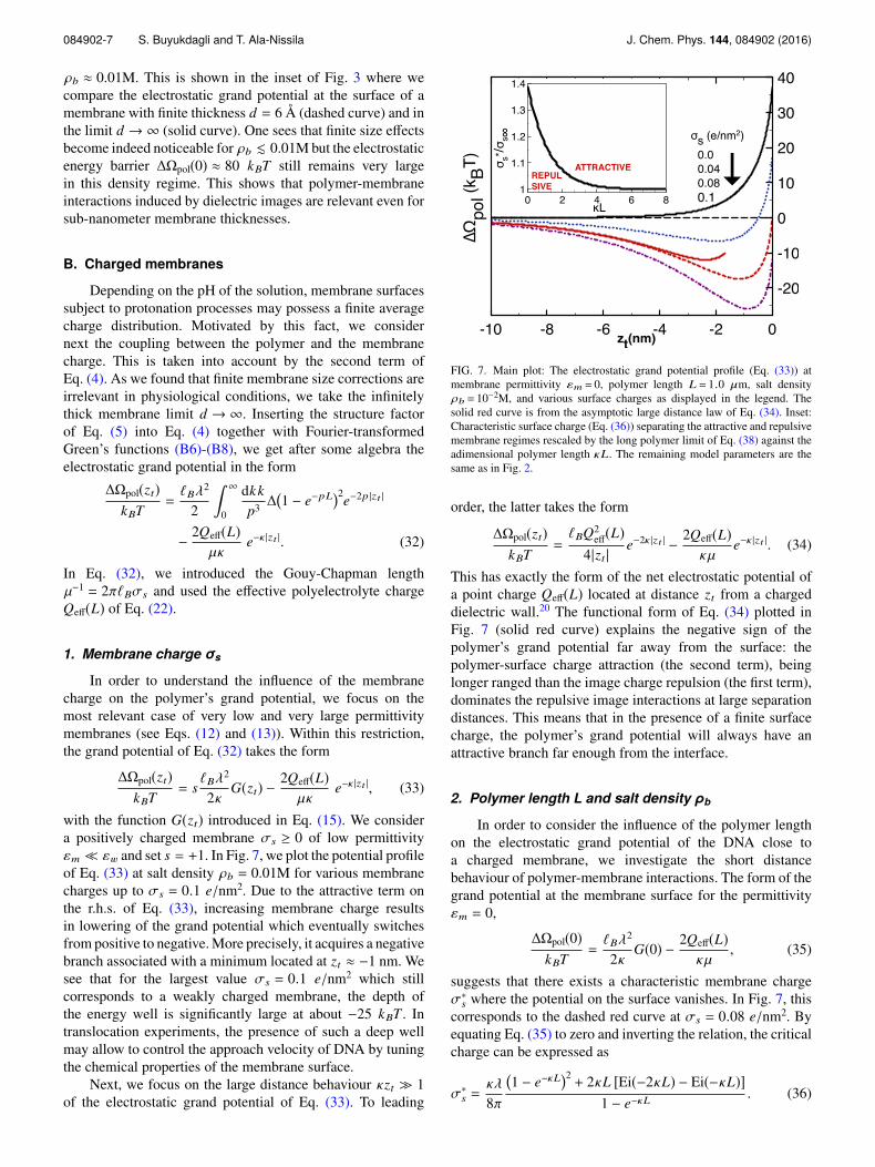
ρb ≈ 0.01M. This is shown in the inset of Fig. 3 where wecompare the electrostatic grand potential at the surface of amembrane with finite thickness d = 6 Å (dashed curve) and inthe limit d → ∞ (solid curve). One sees that finite size effectsbecome indeed noticeable for ρb . 0.01M but the electrostaticenergy barrier ∆Ωpol(0) ≈ 80 kBT still remains very largein this density regime. This shows that polymer-membraneinteractions induced by dielectric images are relevant even forsub-nanometer membrane thicknesses.

B. Charged membranes

Depending on the pH of the solution, membrane surfacessubject to protonation processes may possess a finite averagecharge distribution. Motivated by this fact, we considernext the coupling between the polymer and the membranecharge. This is taken into account by the second term ofEq. (4). As we found that finite membrane size corrections areirrelevant in physiological conditions, we take the infinitelythick membrane limit d → ∞. Inserting the structure factorof Eq. (5) into Eq. (4) together with Fourier-transformedGreen’s functions (B6)-(B8), we get after some algebra theelectrostatic grand potential in the form

∆Ωpol(zt)kBT

=ℓBλ

2

2

∞

0

dkkp3 ∆

1 − e−pL

2e−2p |zt |

− 2Qeff(L)µκ

e−κ |zt |. (32)

In Eq. (32), we introduced the Gouy-Chapman lengthµ−1 = 2πℓBσs and used the effective polyelectrolyte chargeQeff(L) of Eq. (22).

1. Membrane charge σs

In order to understand the influence of the membranecharge on the polymer’s grand potential, we focus on themost relevant case of very low and very large permittivitymembranes (see Eqs. (12) and (13)). Within this restriction,the grand potential of Eq. (32) takes the form

∆Ωpol(zt)kBT

= sℓBλ

2

2κG(zt) − 2Qeff(L)

µκe−κ |zt |, (33)

with the function G(zt) introduced in Eq. (15). We considera positively charged membrane σs ≥ 0 of low permittivityεm ≪ εw and set s = +1. In Fig. 7, we plot the potential profileof Eq. (33) at salt density ρb = 0.01M for various membranecharges up to σs = 0.1 e/nm2. Due to the attractive term onthe r.h.s. of Eq. (33), increasing membrane charge resultsin lowering of the grand potential which eventually switchesfrom positive to negative. More precisely, it acquires a negativebranch associated with a minimum located at zt ≈ −1 nm. Wesee that for the largest value σs = 0.1 e/nm2 which stillcorresponds to a weakly charged membrane, the depth ofthe energy well is significantly large at about −25 kBT . Intranslocation experiments, the presence of such a deep wellmay allow to control the approach velocity of DNA by tuningthe chemical properties of the membrane surface.

Next, we focus on the large distance behaviour κzt ≫ 1of the electrostatic grand potential of Eq. (33). To leading

FIG. 7. Main plot: The electrostatic grand potential profile (Eq. (33)) atmembrane permittivity εm = 0, polymer length L = 1.0 µm, salt densityρb = 10−2M, and various surface charges as displayed in the legend. Thesolid red curve is from the asymptotic large distance law of Eq. (34). Inset:Characteristic surface charge (Eq. (36)) separating the attractive and repulsivemembrane regimes rescaled by the long polymer limit of Eq. (38) against theadimensional polymer length κL. The remaining model parameters are thesame as in Fig. 2.

order, the latter takes the form

∆Ωpol(zt)kBT

=ℓBQ2

eff(L)4|zt | e−2κ |zt | − 2Qeff(L)

κµe−κ |zt |. (34)

This has exactly the form of the net electrostatic potential ofa point charge Qeff(L) located at distance zt from a chargeddielectric wall.20 The functional form of Eq. (34) plotted inFig. 7 (solid red curve) explains the negative sign of thepolymer’s grand potential far away from the surface: thepolymer-surface charge attraction (the second term), beinglonger ranged than the image charge repulsion (the first term),dominates the repulsive image interactions at large separationdistances. This means that in the presence of a finite surfacecharge, the polymer’s grand potential will always have anattractive branch far enough from the interface.

2. Polymer length L and salt density ρb

In order to consider the influence of the polymer lengthon the electrostatic grand potential of the DNA close toa charged membrane, we investigate the short distancebehaviour of polymer-membrane interactions. The form of thegrand potential at the membrane surface for the permittivityεm = 0,

∆Ωpol(0)kBT

=ℓBλ

2

2κG(0) − 2Qeff(L)

κµ, (35)

suggests that there exists a characteristic membrane chargeσ∗s where the potential on the surface vanishes. In Fig. 7, thiscorresponds to the dashed red curve at σs = 0.08 e/nm2. Byequating Eq. (35) to zero and inverting the relation, the criticalcharge can be expressed as

σ∗s =κλ

8π

1 − e−κL

2+ 2κL [Ei(−2κL) − Ei(−κL)]

1 − e−κL. (36)

084902-8 S. Buyukdagli and T. Ala-Nissila J. Chem. Phys. 144, 084902 (2016)

We plot Eq. (36) in the inset of Fig. 7. Increasing the reducedpolymer length κL, the critical charge drops smoothly from

σs0 ≈ 2 ln(2) κλ8π

, (37)

for κL ≪ 1 to

σs∞ ≈κλ

8π, (38)

for κL ≫ 1. We note that in both limits the characteristiccharge is independent of the polymer length.

We consider next the length dependence of theelectrostatic grand potential of Eq. (35). For short polymersκL ≪ 1, it takes the asymptotic form

∆Ωpol(0)∆Ω∗

≈ 2 ln(2)1 − σs

σs0

κL (39)

which switches from repulsive to attractive at σs = σs0. Forlong polymers κL ≫ 1, the grand potential reads

∆Ωpol(0)∆Ω∗

≈ 1 − σs

σs∞(40)

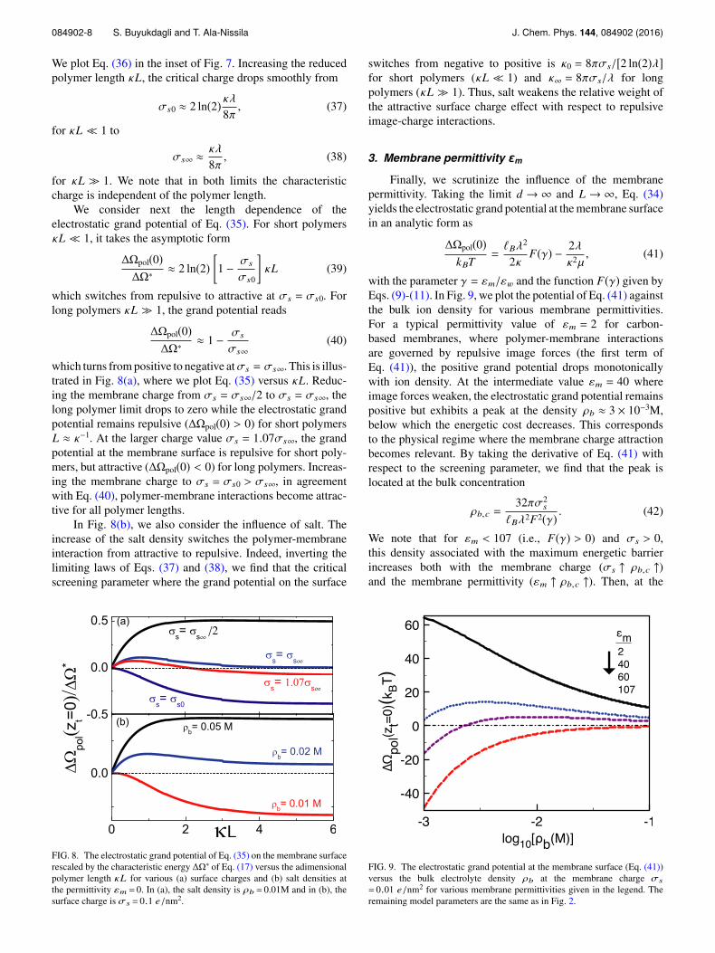
which turns from positive to negative atσs = σs∞. This is illus-trated in Fig. 8(a), where we plot Eq. (35) versus κL. Reduc-ing the membrane charge from σs = σs∞/2 to σs = σs∞, thelong polymer limit drops to zero while the electrostatic grandpotential remains repulsive (∆Ωpol(0) > 0) for short polymersL ≈ κ−1. At the larger charge value σs = 1.07σs∞, the grandpotential at the membrane surface is repulsive for short poly-mers, but attractive (∆Ωpol(0) < 0) for long polymers. Increas-ing the membrane charge to σs = σs0 > σs∞, in agreementwith Eq. (40), polymer-membrane interactions become attrac-tive for all polymer lengths.

In Fig. 8(b), we also consider the influence of salt. Theincrease of the salt density switches the polymer-membraneinteraction from attractive to repulsive. Indeed, inverting thelimiting laws of Eqs. (37) and (38), we find that the criticalscreening parameter where the grand potential on the surface

FIG. 8. The electrostatic grand potential of Eq. (35) on the membrane surfacerescaled by the characteristic energy ∆Ω∗ of Eq. (17) versus the adimensionalpolymer length κL for various (a) surface charges and (b) salt densities atthe permittivity εm = 0. In (a), the salt density is ρb = 0.01M and in (b), thesurface charge is σs = 0.1 e/nm2.

switches from negative to positive is κ0 = 8πσs/[2 ln(2)λ]for short polymers (κL ≪ 1) and κ∞ = 8πσs/λ for longpolymers (κL ≫ 1). Thus, salt weakens the relative weight ofthe attractive surface charge effect with respect to repulsiveimage-charge interactions.

3. Membrane permittivity εmFinally, we scrutinize the influence of the membrane

permittivity. Taking the limit d → ∞ and L → ∞, Eq. (34)yields the electrostatic grand potential at the membrane surfacein an analytic form as

∆Ωpol(0)kBT

=ℓBλ

2

2κF(γ) − 2λ

κ2µ, (41)

with the parameter γ = εm/εw and the function F(γ) given byEqs. (9)-(11). In Fig. 9, we plot the potential of Eq. (41) againstthe bulk ion density for various membrane permittivities.For a typical permittivity value of εm = 2 for carbon-based membranes, where polymer-membrane interactionsare governed by repulsive image forces (the first term ofEq. (41)), the positive grand potential drops monotonicallywith ion density. At the intermediate value εm = 40 whereimage forces weaken, the electrostatic grand potential remainspositive but exhibits a peak at the density ρb ≈ 3 × 10−3M,below which the energetic cost decreases. This correspondsto the physical regime where the membrane charge attractionbecomes relevant. By taking the derivative of Eq. (41) withrespect to the screening parameter, we find that the peak islocated at the bulk concentration

ρb,c =32πσ2

s

ℓBλ2F2(γ) . (42)

We note that for εm < 107 (i.e., F(γ) > 0) and σs > 0,this density associated with the maximum energetic barrierincreases both with the membrane charge (σs ↑ ρb,c ↑)and the membrane permittivity (εm ↑ ρb,c ↑). Then, at the

FIG. 9. The electrostatic grand potential at the membrane surface (Eq. (41))versus the bulk electrolyte density ρb at the membrane charge σs

= 0.01 e/nm2 for various membrane permittivities given in the legend. Theremaining model parameters are the same as in Fig. 2.

084902-9 S. Buyukdagli and T. Ala-Nissila J. Chem. Phys. 144, 084902 (2016)

FIG. 10. Phase diagram: the membrane charge (Eq. (43)) versus salt densityρb for various membrane permittivities. The characteristic curves split theregions associated with repulsive membranes (above the curves) and attractivemembranes (below the curves). The remaining model parameters are the sameas in Fig. 2.

permittivity value εm = 60, the polymer grand potential ispositive at biological salt concentrations but negative fordilute electrolytes. Finally, at the value εm = 107 (and forlarger permittivities), because image interactions switch fromrepulsive to attractive, i.e., F(γ) ≤ 0 (see also Fig. 3), themembrane becomes purely attractive at all salt densities.

For translocation experiments carried out with differentmembrane types, it is interesting to characterize the physicalregime where the energy barrier at the membrane surfacevanishes. Setting Eq. (41) to zero, we find that this occurs atthe characteristic membrane charge

σ∗s =κλ

8πF(γ). (43)

We note that Eq. (43) generalizes the limiting law of Eq. (38)to any permittivity value εm. Based on Eq. (43), we showin Fig. 10 the phase diagram characterizing the parameterregimes with attractive membranes (area above each curve)and repulsive membranes (area below each curve). In thisfigure, the switching of the membrane charge to negativefrom up to bottom stems from the fact that the attractiveimage forces for εm > 107 have to be compensated by therepulsion between the negative membrane charge and thenegative polymer charge in order for the net surface grandpotential to cancel out.

The phase diagram in Fig. 10 indicates that at constantmembrane permittivity, the larger the electrolyte density,the larger the characteristic membrane charge where theelectrostatic grand potential on the surface vanishes. Indeed,we have shown above that the attractive force induced by thesurface charge is more susceptible to salt screening than imageforces (see, e.g., Fig. 8(b)). Thus, a stronger salt density has tobe compensated by a stronger membrane charge to cancel outthe net free at the membrane surface. Furthermore, at constantsalt concentration, the larger the dielectric discontinuity, thestronger the surface charge. In translocation experiments,the complex picture of this phase diagram can be at least

qualitatively checked by observing the approach of a DNAmolecule towards membranes with different chemical surfaceproperties.

III. SUMMARY AND CONCLUSIONS

In this work, we have developed an analytical theoryaccounting for electrostatic membrane-polymer interactionsduring the approach phase of DNA translocation events. Thecorresponding DH theory goes beyond the mean field approx-imation as it includes correlation effects such as image-chargeinteractions resulting from the dielectric mismatch between themembrane and the surrounding solvent. Within this theory, wehave characterized the complex interplay between the poly-electrolyte length, the salt density, the membrane dielectricpermittivity, and the membrane charge and size.

In the first part, we considered neutral membranes. Wefound that in the case of thick membranes, whose permittivitystrongly differs from the solvent permittivity, the approach ofa long DNA molecule to the membrane costs the electrostaticgrand potential of magnitude |∆Ωpol(0)| = kBTℓBλ2/(2κ),where λ is the linear DNA charge density. For neutralcarbon-based membranes with low dielectric permittivity(εm ≈ 2), this corresponds to a high energy barrier between10 kBT to 100 kBT depending on the salt concentration.Interestingly, the theory predicts that in the opposite case ofengineered membranes with high permittivity εm ≫ εw,17,18

the membrane surface becomes an attraction point. Moreprecisely, within the physiological salt density regime, theapproach of the polymer to the membrane reduces its grandpotential by 10–100 kBT . We also found that in pure solvents,the electrostatic grand potential becomes independent of thepolymer length if the latter exceeds the membrane thickness,i.e., L ≥ d. In electrolytes, finite size effects related tothe polyelectrolyte length die out if the polymer length islarger than the DH screening length, that is, L ≥ κ−1. Mostimportantly, we showed that for the thinnest graphene-basedmembranes of thickness d ≈ 6 Å,21 the grand potential barrierencountered by the DNA is close to 100 kBT . This indicatesthat surface polarization effects studied herein are crucial evenfor subnanometer membrane sizes.

In the second part, we took into account the finite chargedistribution on the membrane surface. We found that even forweakly charged low permittivity membranes, the electrostaticgrand potential acquires an attractive branch far enough fromthe interface and turns to repulsive very close to the membrane.Because the membrane charge attraction is more sensitive tosalt screening than repulsive image forces, the increase ofthe salt concentration makes the membrane less attractive.Furthermore, due to the competition between membranecharge and image charge effects, the sign of the polymer grandpotential may depend on the polymer length. We showed thatfor specific values of the membrane charge and ion density,the membrane will repel short polymers (L ≪ κ−1) but attractlong polymers (L ≫ κ−1). We also showed that the samecompetition may cancel the net electrostatic grand potentialon the membrane surface, which we characterized in thephase diagram of Fig. 10 in terms of the salt density, andthe membrane charge and permittivity. This phase diagram

084902-10 S. Buyukdagli and T. Ala-Nissila J. Chem. Phys. 144, 084902 (2016)

and our general conclusions can be tested in translocationexperiments.

Finally, we would like to point out limitations in thepresent modeling. In our first attempt to model electrostaticpolymer-membrane interactions, we opted for an evaluationof the polymer’s grand potential at the DH level. Our choiceis motivated by the analytical transparency of the DH theory.It should be of course emphasized that our quadratic DH leveltheory neglects non-linear electrostatic interactions. In dilutesolutions with bulk density ρb . 0.01M, the DH approxi-mation is known to overestimate the electrostatic potentialinduced by charged sources. Hence, at low electrolyte concen-trations, our grand potential curves may overestimate theactual electrostatic energy barrier values. This limitation canbe overcome in a future work by including the non-linearity ofthe electrostatic potential thorough a charge renormalisationprocedure20 or a one-loop evaluation of the grand potential.24

However, it should be noted that such improvements willinvolve considerable complexity and mask the transparencyof the present theory. Furthermore, the rigid polymer modelneglects the entropic fluctuations of the DNA molecule. Thedouble-stranded DNA molecule has a persistence length ofabout 50 nm, and in the case of low permittivity membranesimage charge interactions are expected to greatly enhance it.This justifies our rigid polymer approximation in the mostrelevant case of carbon-based membranes. The importance ofthe role played by polymer fluctuations on DNA-membraneinteractions can be evaluated in a future work by consideringthe polymer entropy through a coupling of the Coulomb liquidmodel with the beyond-MF formulation of the Flory theory.9

We also note that in the present work, we focused exclusivelyon the approach phase of translocation events. In the futurewe would like to extend our theory to the translocation phase,consider dynamical issues, and include hydrodynamic trans-port. We emphasize that despite the limitations of the presenttheory, our main conclusions can be tested in translocationexperiments and the theory can hopefully present itself as astarting point for more sophisticated models. The mappingbetween the membrane dielectric properties and the polymergrand potential that we identified in this work may also allowto improve our control over DNA-membrane interactions viathe chemical engineering of membrane materials.

ACKNOWLEDGMENTS

This work has been supported in part by AaltoUniversity’s Energy Efficiency project EXPECTS. T.A.-N.has also been supported by the Academy of Finland throughits COMP Center of Excellence Grant No. 284621.

APPENDIX A: DEBYE-HÜCKEL LEVELGRAND POTENTIAL

We present here the DH expansion of the grand potentialof the electrolyte. The theory is formulated for general chargedistributions in Ref. 23 and thus we will present only thegeneral lines of the derivation. The grand canonical partitionfunction of the charged liquid is given by the functionalintegral23

ZG =

Dφ e−H [φ], (A1)

with the Hamiltonian functional

H[φ] =

dr

ϵ(r)2βe2 [∇φ(r)]2 − iσ(r)φ(r) −

i

λi eiqiφ(r),

(A2)

where r stands for the position vector, β = 1/(kBT) is theinverse temperature, e the electron charge, and ϵ(r) thedielectric permittivity function. Moreover, the function σ(r)accounts for immobile charge distributions in the system. Thesummation in the third term of Eq. (A2) runs over the ionicspecies of the electrolyte, each with fugacity λi and valency qi.Finally, within the same field-theoretic representation, localion densities are given by

ρi(r) = λi

eiqiφ(r)

φ, (A3)

where the bracket ⟨·⟩φ denotes the average over fluctuatingpotential configurations taken with respect to the func-tional (A2).

The DH approximation consists in Taylor expandingthe functional (A2) at the quadratic order in the fluctuatingpotential φ(r). One gets the DH functional in the form

H0[φ] =

drϵ(r)2βe2 [∇φ(r)]2 − iσ(r)φ(r)

− V

i

λi

+i

λi

dr

−iqiφ(r) + q2

i

2φ2(r)

. (A4)

As discussed in the Conclusion, the above approximation isvalid at large monovalent salt densities. In dilute salt wherethe electrostatic potential becomes large, the Taylor expansionshould be performed around the solution of the non-linear PBequation.24 Evaluating now in the bulk region ion density (A3)within the same DH approximation gives

ρi,b = λi

1 + iqi⟨φ(r)⟩φ −

q2i

2φ2(r)

φ

b, (A5)

where the subscript b means that the field theoretic averagesshould be evaluated in bulk, i.e., far from any chargedmacromolecules breaking the spherical symmetry of theelectrolyte. Noting that the average electric field should bezero in bulk, i.e., ⟨φ(r)⟩φ,b = 0, and inverting Eq. (A5) in theDH approximation gives

λi = ρi,b *,1 +

q2i

2vDH,b+

-, (A6)

where we defined the bulk limit of the DH Green’s functionvDH,b =

φ2(r) for r in the bulk region. By inserting into

Eq. (A4) the expression for fugacity (A6) together withthe electroneutrality condition

i ρibqi = 0, neglecting the

terms beyond the one-loop level, and restricting ourselvesto the case of a symmetric electrolyte composed of twoionic species with ρ+b = ρ−b = ρb and q+ = −q− = q, theHamiltonian functional becomes

H0[φ] =

drdr′

2φ(r)v−1

DH(r,r′)φ(r′) − i

drσ(r)φ(r), (A7)

084902-11 S. Buyukdagli and T. Ala-Nissila J. Chem. Phys. 144, 084902 (2016)

where we defined the DH kernel as

v−1DH(r,r′) =

− 1βe2∇ · ε(r)∇ + 2ρbq2

δ(r − r′). (A8)

We note that deriving Eq. (A8), we dropped the constant termV

i λi in Eq. (A4) and the term linear in the potential φ(r)

disappeared due to the electroneutrality condition. Computingthe DH-level partition function with Eqs. (A1) and (A7) gives

Z0 = det1/2 (vDH) exp−

drdr′

2σ(r)vDH(r,r′)σ(r′)

. (A9)

From the definition of the grand potential ΩDH = −kBT ln Z0,we finally get the latter as the superposition of the ionic andpolymer free energies ΩDH = Ωion +Ωpol, each contribution,respectively, given by Ωion = −kBT ln det1/2 (vDH) and

Ωpol = kBT

drdr′

2σ(r)vDH(r,r′)σ(r′). (A10)

APPENDIX B: ELECTROSTATIC GREEN’S FUNCTIONIN SLIT GEOMETRY

In this Appendix, we explain the general lines of theinversion of DH kernel equation (A8) in the planar membranegeometry depicted in Fig. 1. Due to the plane geometry wherethe Green’s function satisfies translational symmetry alongthe x and the y axes, i.e., vDH(r,r′) = vDH(z, z′,r∥ − r′∥), wecan Fourier-expand the Green’s function as

vDH(r,r′) =

d2k4π2 e

ik·(r∥−r′∥

)vDH(z, z′). (B1)

In Eq. (B1), the dependence of the Fourier expanded Green’sfunction on the wave vector k is implicit. Moreover, thedielectric permittivity profile reads

ε(z) = εwθ(−z) + εmθ(z)θ(d − z) + εwθ(z − d), (B2)

where θ(z) is the Heaviside step function. By inserting theexpansion (B1) into the kernel equation (A8), the lattersimplifies as

∂zε(z)∂z − p2 vDH(z, z′) = − e2

kBTδ(z − z′), (B3)

with p =√

k2 + κ2 and the DH screening parameterκ = 8πq2ℓBρb. For the source charge located on the rightside of the membrane z′ > d, the piecewise homogeneoussolution is

vDH(z, z′) = C1epzθ(−z) + C2ekz + C3e−kzθ(z)θ(d − z)

+C4epz + C5e−pz

θ(z − d)θ(z′ − z)

+C6e−pzθ(z − z′). (B4)

For the source located in the left half-space z′ < 0, the solutionis given by

vDH(z, z′) = C1epzθ(z′ − z)+C2epz + C3e−pz

θ(−z)θ(z − z′)

+C4ekz + C5e−kz

θ(z)θ(d − z)

+C6e−pzθ(z − d). (B5)

The integration constants Ci with 1 ≤ i ≤ 6 are to bedetermined by applying in each case the continuity ofthe Green’s function vDH(z, z′) and the displacement fieldε(z)∂z vDH(z, z′) at the boundaries z = 0, z = d, and at z = z′.After somewhat tedious algebra we get

vDH(z ≤ 0, z′ ≤ 0) = vb(z − z′) + 2πℓBp∆1 − e−2kd

1 − ∆2e−2kd ep(z+z′),

(B6)

vDH(z ≥ d, z′ ≥ d) = vb(z − z′)

+2πℓB

p∆1 − e−2kd

1 − ∆2e−2kd ep(2d−z−z′), (B7)

and

vDH(z, z′) = vb(z − z′) + 2πℓBp

× (1 − ∆2)e(p−k)d + ∆2e−2kd − 11 − ∆2e−2kd e−p |z−z

′|, (B8)

for z′ ≤ 0 and z ≥ d, or z′ ≥ d and z ≤ 0. In Eqs. (B6)-(B8),the dielectric discontinuity function is defined as

∆ =εwp − εmkεwp + εmk

. (B9)

We finally note that in Eqs. (B6)–(B8), we introduced the bulkpart of the Fourier transformed DH Green’s function

vb(z − z′) = 2πℓBp

e−p |z−z′|. (B10)

1M. Hi, The Cell Cycle: Principles of Control (New Science Press, London,2007).

2B. Alberts, Molecular Biology of the Cell (Garland Science, New York,2002).

3N. X. Wang and H. A. von Recum, Macromol. Biosci. 11, 321 (2011).4D. H. Kaye, The Double Helix and the Law of Evidence (Harvard UniversityPress, Massachusetts, 2010).

5S. F. Edwards, Proc. Phys. Soc. 85, 613 (1965).6R. Podgornik and B. Zeks, J. Chem. Soc., Faraday Trans. 2 84, 611 (1988).7R. Podgornik, Chem. Phys. Lett. 174, 191 (1990).8R. Podgornik, J. Phys. Chem. 95, 5249 (1991).9S. Tsonchev, R. D. Coalson, and A. Duncan, Phys. Rev. E 60, 4257 (1999).

10H. Seki, Y. Y. Suzuki, and H. Orland, J. Phys. Soc. Jpn. 76, 104601 (2007).11R. Kumar and M. Muthukumar, J. Chem. Phys. 131, 194903 (2009).12S. Buyukdagli and T. Ala-Nissila, Langmuir 30, 12907 (2014).13S. Qiu, Y. Wang, B. Cao, Z. Guo, Y. Chen, and G. Yang, Soft Matter 11, 4999

(2015).14S. Buyukdagli, R. Blossey, and T. Ala-Nissila, Phys. Rev. Lett. 114, 088303

(2015).15C.-H. Cheng and P.-Y. Lai, Phys. Rev. E 70, 061805 (2004).16A. G. Cherstvy and R. G. Winkler, J. Phys. Chem. B 116, 9838 (2012).17Z. M. Dang, L. Wang, Y. Yin, Q. Zhang, and Q. Q. Lei, Adv. Mater. 19, 852

(2007).18A. Dimiev, D. Zakhidov, B. Genorio, K. Oladimeji, B. Crowgey, L. Kempel,

E. J. Rothwell, and J. M. Tour, Appl. Mater. Interfaces 5, 567 (2013).19M. Abramowitz and I. A. Stegun, Handbook of Mathematical Functions

(Dover Publications, New York, 1972).20S. Buyukdagli, M. Manghi, and J. Palmeri, Phys. Rev. E 81, 041601 (2010).21S. Garaj, W. Hubbard, A. Reina, J. Kong, D. Branton, and J. A. Golovchenko,

Nature 467, 190 (2010).22H. Chang, F. Kosari, G. Andreadakis, M. A. Alam, G. Vasmatzis, and R.

Bashir, Nano Lett. 4, 1551 (2004).23R. R. Netz, Eur. Phys. J. E 5, 189 (2001).24S. Buyukdagli, C. V. Achim, and T. Ala-Nissila, J. Chem. Phys. 137, 104902

(2012).