Embed Size (px)
Citation preview

Journal of hternationd Mone_p and Finance (199 I), 10, 7 l-88
Business cycles, stylized facts, and the exchange rate regime: evidence from the
United States
MARIANNE BAXTER*
Department of Economics, Unicersity of Rochester, Rochester, NY 14627, USA
This paper investigates the robustness of central macroeconomic ‘stylized facts’ to (i) commonly-employed detrending methods, and (ii) the exchange rate regime. We find that the stylized facts are not at all robust to the choice of detrending method, with the most important variations occurring in the cyclic behavior of hours and productivity. With respect to the exchange rate regime, the most surprising find is that the correlation between GNP, on the one hand, and consumption, investment, hours, exports, and imports on the other, all rose in the post-1973 period. This reinforces Baxter and Stockman’s (1989) finding that business cycles in the post-1973 period have been more nation-specific than in the prior Bretton-Woods era.
The postwar period has been characterized by two distinct exchange rate regimes: the fixed rate Bretton Woods system, established in 1944, and the floating rate period which dates from 1973. Most international macroeconomists believe that the exchange rate regime is of prime importance in understanding the domestic effects and international transmission of variations in government policy. Indeed, Frenkel and Razin (1987, p. 450) state that ‘The so-called Mundell-Fleming model is still the main workhorse of international open-economy macro- economics.’ The simple Mundell-Fleming model has been extended in many directions,’ but in virtually all versions of that model the international trans- mission mechanisms depend critically on the exchange rate regime.
It is therefore troubling that most empirical research in macroeconomics implicitly treats data from the postwar period as if they were generated by a single stochastic process. This assumption is made whenever a model is evaluated using data from the entire postwar period with no explicit allowance made for differences between the pre-1973 versus the post-1973 periods. Typically these models are attempting to explain the behavior of US time series, and the assumption implicit in this modeling strategy is that the US economy is so large that it is approximately a closed economy. But this assumption is increasingly untenable as international capital markets become more integrated, and as the
* Thanks are due to Robert King, James Lothian, Kenneth Rogoff. and a referee for discussions and comments which materially influenced the direction of this paper. They are not, however, responsible for its contents or conclusions. The support of the National Science Foundation under grant SES-8606758 is gratefully acknowledged.
0261-5606:91/01/0071-18 C 1991 Butterworth-Heinemann Ltd

72 Business cp-les and st,vlked facts
relative importance of the US in the world economy declines. This criticism applies equally to atheoretical macroeconometric models, ‘new-Keynesian’ models, and equilibrium business cycle models.
Further, there is abundant evidence that at least one real variable-the real exchange rate-exhibits dramatically different behavior under fixed and flexible exchange rate regimes. Mussa (1986) provides extensive documentation of the fact that the real exchange rate is much more volatile under flexible rates, and that it in fact behaves very much like the nominal exchange rate. Since the real exchange rate is viewed as the relative price of national outputs, such a dramatic difference in the volatility of this relative price across exchange rate regimes suggests that there should exist similarly dramatic cross-regime differences in the behavior of national outputs, consumption, investment, and labor supply.
Yet Baxter and Stockman (1989) recently reported that, in OECD data, it is difficult to find important cross-regime differences in the behavior of real macroaggregates such as output, consumption, and investment.* In a sample of 44 countries (including many LDCs) they found that the volatility of the real exchange rate and the levels of trade activity were both higher after 1973, but appeared to be unrelated to a country’s choice of exchange rate regime. They concluded that these results presented a puzzle from the point ofview oftraditional international macroeconomic theory. The present paper complements the Baxter and Stockman (1989) investigation and a related study (Gerlach, 1988) by providing a detailed analysis of the cross-regime behavior of the largest economy in the world-that of the United States. By focusing on a single country, we can investigate time series at a lower level of aggregation than in those analyses, and can potentially uncover cross-regime differences which were masked by the high levels of aggregation used in prior studies.
The goal of this paper is to determine whether the statistical behavior of US macroeconomic aggregates has changed substantially in the post-1973 flexible rate period, compared with the earlier, fixed rate period. Knowing the answer to this question is important to building empirically relevant models of the US economy. While the results of this investigation should be useful in determining which classes of theories are likely to provide a better fit to the data, the goal of this paper is not to test specific theories. In the concluding section of this paper, however, we discuss the implications of this work for future model-building and model-evaluation activities.
The paper is organized as follows. Section I provides an overview of the ‘stylized facts’ of the US macroeconomy, defined as the salient patterns of volatility and comovement of important macroeconomic aggregates. This section examines the sensitivity to detrending procedures of the stylized facts that are commonly used to evaluate the empirical adequacy of theoretical models. It is unfortunate that there is no agreement among researchers on the appropriate method for removing nonstationary components from macroeconomic time series. Singleton (1988) has argued that the data should be treated in a manner consistent with the model under study, but sometimes this is impossible (for example, if there is no source of nonstationarity in the model). It is even more unfortunate that the stylized facts themselves are sensitive to choice of detrending procedure. This section presents evidence on the non-robustness of the stylized facts to detrending procedures, and attempts to interpret the source of these differences.
Section II investigates whether the statistical behavior of key macroaggregates

MARIANNE BAXTER 73
depends in a systematic way on the exchange rate regime. The lesson from Section II is that we cannot discuss this issue separately from the detrending issue. This section therefore presents results for a variety of commonly employed detrending methods. Section III contains a summary of the paper’s main results, and Section IV concludes the paper with a discussion of implications for the practice of closed and open economy macroeconomics.
I. Detrending procedures and the stylized facts
The first detailed statistical analyses of business cycles were undertaken in the 1920s by the National Bureau of Economic Research under the leadership of Wesley Clair Mitchell. Eschewing traditional statistical methodology, Mitchell and his collaborators developed new methods for summarizing business cycle phenomena. They found that the empirical regularities of economic fluctuations lay not in the length of cycle or its amplitude, but rather in the patterns of comovement (conformity) and relative amplitude of economic variables. Morgenstem (1959) carried out detailed analyses of international business cycles, and raised the question of whether the international character and transmission of cycles depended on the exchange rate regime.
Mitchell’s method of summarizing business fluctuations involved computing statistics based on the reference cycle construct. The dates of business cycle peaks and troughs were first determined with a procedure that involved a substantial degree of judgment which, consequently, is difficult to replicate. Then, individual series were examined for ‘specific cycles.’ Each time series was expressed as a deviation from its specific cycle average, removing aspects of trend. Various measures of amplitude, comovement, and lead-lag relations were then computed.
More recently, the neoclassical approach to studying business cycles has generally abstained from dating ofcycles. More conventional statistical measures are typically used to evaluate model adequacy, which requires that some stationarity-inducing transformation be applied to the data. Two commonly used detrending procedures are (i) removal of a log-linear trend and (ii) taking first differences of logs.
An alternative detrending method has been proposed by Hodrick and Prescott (1980), in perhaps the most widely cited unpublished paper in macroeconomics. Their objective was ‘to examine the magnitudes and stability of covariances between various economic time series and real output and the autocovariances of real output’ (1980, p. 2). Hodrick and Prescott employed an unusual filter- their filter is two-sided, and removes a ‘trend’ that resembles a smooth curve drawn through the data. Figure 1 graphs the log of US real exports and the trend component which would be removed by application of the Hodrick-Prescott (HP) filter. This figure shows clearly the potential for the HP filter to produce a nonmonotonic trend component.
Prescott (1986) indicates that statistics generated by the HP filter are similar to those computed after applying a band-pass filter which removes cycles of period greater than about 32 quarters. So there is a sense in which the HP filter isolates ‘business cycle phenomena,’ if these are interpreted as cycles in the data of period less than about three years.
Since all three of these detrending procedures are commonly used to isolate empirical ‘business cycles’ for the purpose of model evaluation, we first examine
73 Business cycles and srylid facts
&Or
Log of real exports: actual and HP filtered
h-T
50
t - Real exports
5,6_ ---- I-PtrerKl
5.4-
5.2-
5.0 -
4.2
4.01 r I I I I I I 1 1945 1950 1955 1960 1965 I970 1975 1980 1985 19
Date
FIGURE 1.
Ql 3
the robustness to detrending method of key business cycle statistics. Prescott (1986, p. 13) states that ‘If the business-cycle facts were sensitive to the detrending procedure employed, there would be a problem; but the key facts are not sensitive to the procedure if the trend curve is smooth.’ Our results show that Prescott is mistaken: we find that many of these statistics are very sensitive to the method of detrending, even within the class of ‘smooth trend’ filters.
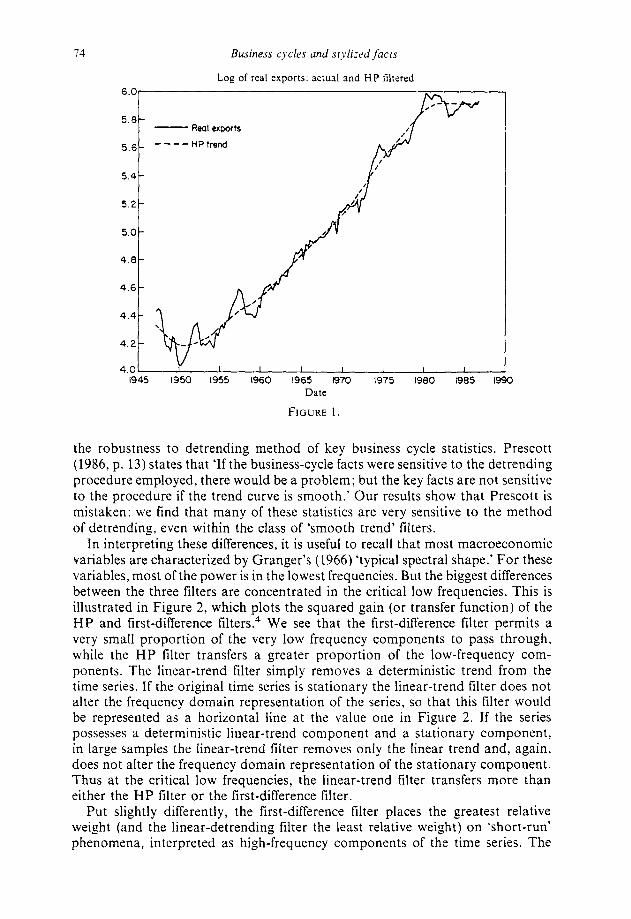
In interpreting these differences, it is useful to recall that most macroeconomic variables are characterized by Granger’s (1966) ‘typical spectral shape.’ For these variables, most of the power is in the lowest frequencies. But the biggest differences between the three filters are concentrated in the critical low frequencies. This is illustrated in Figure 2, which plots the squared gain (or transfer function) of the HP and first-difference filters4 We see that the first-difference filter permits a very small proportion of the very low frequency components to pass through, while the HP filter transfers a greater proportion of the low-frequency com- ponents. The linear-trend filter simply removes a deterministic trend from the time series. If the original time series is stationary the linear-trend filter does not alter the frequency domain representation of the series, so that this filter would be represented as a horizontal line at the value one in Figure 2. If the series possesses a deterministic linear-trend component and a stationary component, in large samples the linear-trend filter removes only the linear trend and, again, does not alter the frequency domain representation of the stationary component. Thus at the critical low frequencies, the linear-trend filter transfers more than either the HP filter or the first-difference filter.
Put slightly differently, the first-difference filter places the greatest relative weight (and the linear-detrending filter the least relative weight) on ‘short-run’ phenomena, interpreted as high-frequency components of the time series. The
MARIANNE BAXTER 75
The HP and first-difference filters
40 RR
/ 0
0 3 5- - HP filter /
First -dtfference filter /
--_- / /
/ 30- /
/’ /
2.5 - /
E Ek
1’ /
x 2.0- S /’ z /
* l.S- 1’
1’ /
/
01 0.2 0.3 0.4 0.5 0.6 07 0.8 0.9 I Frequency in radians (fractions of pi)
FIGURE 2.
HP filter occupies an intermediate position. This perhaps suggests that we should observe a consistent ordering in the statistics generated through the use of these filters, but we shall see that this is not always the case.
If application of these lilters is viewed as isolating ‘business cycle’ phenomena, it is clear that each filter embeds a different concept of the business cycle, defined as a linear combination of cycles at different frequencies. One interpretation of the lack of professional consensus on the appropriate method of filtering is that we lack a professional consensus on a definition of a ‘business cycle’ which is sufficiently precise to permit representation as a specific filter.
With this background in mind, we turn now to an investigation of the effects of filtering on our beliefs about the ‘stylized facts of business cycles.’ In this paper we study the cyclic behavior of 13 key US aggregate variables. All data are from the Citibase database, and all variables are in real terms (deflated by their own implicit price deflators) unless otherwise noted. In each case, natural logs were taken before detrending.
IA. Volatility
Measures of volatility have long been important business cycle statistics, and are intended to measure the extent of fluctuation in a variable over the business cycle. Mitchell discussed volatility in terms of a variable’s amplitude over the reference cycle. The volatility measure employed in this paper is the standard deviation of detrended data, which is a measure of volatility more commonly used by modern researchers.5
Table 1 presents the standard deviations of the 13 US time series under study.
76 Business cycles and stylized facts
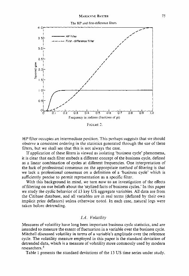
TABLE 1. Volatility statistics’ (quarterly data, 1947:l to 1986:3).
Detrending method
Variable Linear trend HP filter First difference
GNP 4.4 2.0 1.1 Consumption: total 2.8 1.2 0.8 Consumption: services 2.9 0.7 0.6 Consumption: nondurable 3.0 1.2 0.8 Consumption: durables 8.5 5.5 4.2 Gross private domestic investment 11.0 9.1 5.9 Inv. in P&E: total’ 10.0 6.0 3.0 Inv. in P&E: mfg. nondurable 11.6 7.3 4.2 Inv. in P&E: mfg. durable 18.1 11.9 5.5 Hours3 4.1 1.9 1.0 Productivity’ 2.9 1.6 1.2 Exports 12.9 6.3 4.4 Imports 8.4 5.3 4.3
’ Volatility is defined as the standard deviation of detrended data.
’ Investment in plant and equipment.
’ Hours of all persons: business sector.
’ Output per man hour in manufacturing.
Data source: CITIBASE.
Three commonly employed filters were applied to the data: removal of a linear trend, application of the HP filter, and taking first differences. First, we note that the volatility of the ‘cyclic’ (detrended) data varies widely, depending on the detrending method. However, volatility does depend in a predictable way on the detrending procedure. The smallest variances are associated with the tirst- difference filter, the next largest variances are associated with the Hodrick- Prescott filter, and the largest variances are associated with the linear-trend filter. For time series which exhibit Grangqr’s (1966) typical spectral shape, one should expect this uniform ordering of variances across filtering methods. For each filter, the consumption series are the least volatile and the investment and export series are the most volatile.
I.B. Relative volatility
In many empirical studies of business cycles, the volatility measure employed is the variable’s cyclic variance relative to that of GNP. This approach has the virtue of ‘standardizing’ for the severity of the business cycle. Burns and Mitchell (1941) were interested in the amplitudes of various series relative to output. Their plots of reference cycles for output, consumption, and investment bring home forcefully the fact that consumption is much less cyclically volatile than output, and investment is much more volatile. More recently, Kydland and Prescott (1982, p. 1360) state that ‘One cyclical observation is that, in percentage terms, investment varies three times as much as output does and consumption only half as much.’ We have seen that the level of volatility is not robust to detrending

MARIANNE BAXTER
TABLE 2. Relative volatility statistics’ (quarterly data, 1947:l to 1986:3).
77
Detrending method
Variable Linear trend HP filter First difference
GNP Consumption: total Consumption: services Consumption: nondurable Consumption: durables Gross investment’ Inv. in P & E: total3 Inv. in P&E: mfg. nondurable Inv. in P & E: mfg. durable Hours Productivity Exports Imports
1.00 1.00 1.00 0.64 0.60 0.73 0.66 0.35 0.55 0.68 0.60 0.73 1.93 2.75 3.82 2.50 4.55 5.36 2.27 3.00 2.73 2.64 3.65 3.82 4.11 5.95 5.00 0.93 0.95 0.91 0.66 0.80 1.09 2.93 3.15 4.00 1.91 2.65 3.91
’ Relative volatility is defined as the detrended variable’s standard deviation divided by the standard deviation of detrended GNP. * Gross private domestic investment. ’ Investment in plant and equipment.
Data source: CITIBASE.
method. However, it might still be true that relatiw volatility is robust to detrending even though the levels of volatility differ.
Table 2 presents relative volatility measures for the three detrending procedures. Clearly, the relative volatility measures are not any more robust to detrending method than were the levels of volatility. For several variables, relative volatility differs by a factor of about two, depending on the detrending method: examples are consumption of services, purchases of consumer durables, and gross private domestic investment. And while the HP filter yields lecels of volatility which are intermediate between those produced by the linear-trend and differencing filters, this ordering is not preserved when looking at relntice volatilities.6 For example, the HP filter produces relative volatility statistics which are the lowest of the three detrending methods for several measures of consumption (total consump- tion, consumption of services, and consumption of nondurables). Yet the HP filter produces the largest relative volatility statistics for (total and manufacturing durable) investment in plant and equipment and for hours.
At this point, one may object that the ‘stylized facts’ of business cycles are understood to be qualitative phenomena, such as ‘consumption is less volatile than output, and investment is more volatile.’ But our results show that some important qualitative phenomena are not robust to detrending method. With the HP and linear-trend filters, hours exhibit higher (absolute and relative) volatility than productivity, and both hours and productivity are less volatile than output. But for the first-difference filter, volatility of productivity (absolute and relative) is higher than relative volatility of hours, and productivity is in fact more volatile than output. Evidently, even important qualitative features of the data are not robust to detrending method.
78 Business cycles and stylized facts
I.C. Comocement \cith GNP
Another important class of business cycle stylized facts concerns patterns of comovement of various series with ‘the business cycle,’ typically defined as cyclic movements in output. In the Burns and Mitchell methodology, economic variables were discussed in terms of their ‘conformity’ with the business cycle. In modern business cycle research, variables are examined for their auto- covariances with output at various leads and lags.
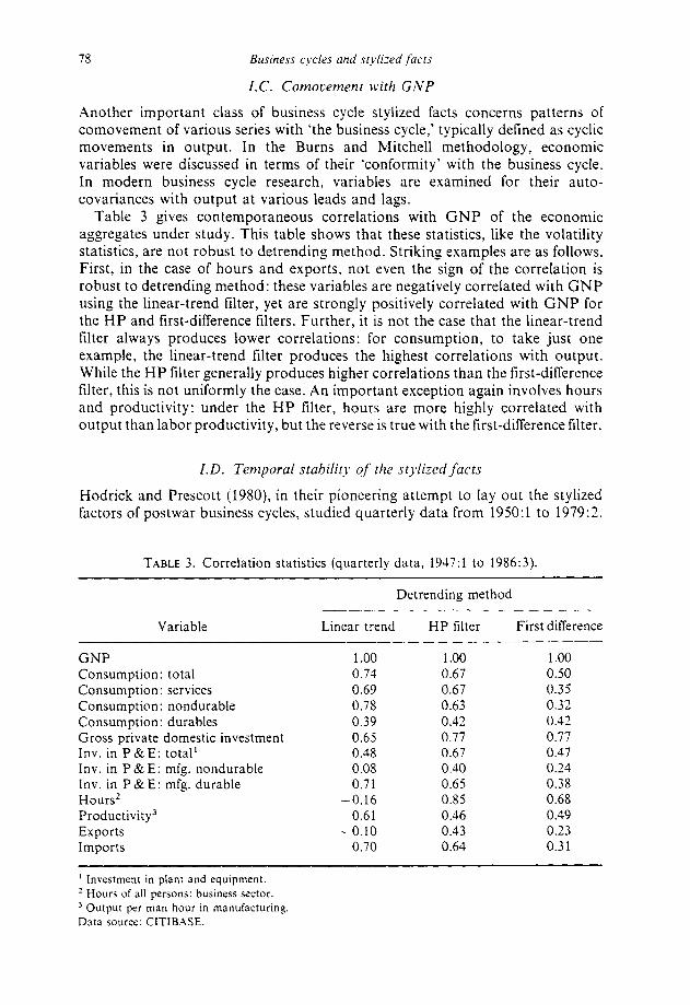
Table 3 gives contemporaneous correlations with GNP of the economic aggregates under study. This table shows that these statistics, like the volatility statistics, are not robust to detrending method. Striking examples are as follows. First, in the case of hours and exports, not even the sign of the correlation is robust to detrending method: these variables are negatively correlated with GNP using the linear-trend filter, yet are strongly positively correlated with GNP for the HP and first-difference filters. Further, it is not the case that the linear-trend filter always produces lower correlations: for consumption, to take just one example, the linear-trend filter produces the highest correlations with output. While the HP filter generally produces higher correlations than the first-difference filter, this is not uniformly the case. An important exception again involves hours and productivity: under the HP filter, hours are more highly correlated with output than labor productivity, but the reverse is true with the first-difference filter.
I.D. Temporal stabilitrl of the stylizeti facts
Hodrick and Prescott (1980), in their pioneering attempt to lay out the stylized factors of postwar business cycles, studied quarterly data from 195O:l to 1979:2.
TABLE 3. Correlation statistics (quarterly data, 1947:l to 1956:3).
Detrending method
Variable Linear trend HP filter First difference
GNP 1 .oo 1 .oo 1 .oo Consumption: total 0.74 0.67 0.50 Consumption: services 0.69 0.67 0.35 Consumption: nondurable 0.78 0.63 0.32 Consumption: durables 0.39 0.42 0.42 Gross private domestic investment 0.65 0.77 0.77 Inv. in P&E: total’ 0.48 0.67 0.47 Inv. in P&E: mfg. nondurable 0.08 0.40 0.24 Inv. in P&E: mfg. durable 0.71 0.65 0.38 Hours’ -0.16 0.85 0.68 Productivity3 0.61 0.46 0.49 Exports -0.10 0.43 0.23 Imports 0.70 0.64 0.31
’ Investment in plant and equipment. ’ Hours of all persons: business sector.
’ Output per man hour in manufacturing.
Data source: CITIBASE.

MARIANNE BAXTER 79
As part of their analysis, they constructed a statistic which measures the stability across the two halves of the sample of the relationship between the variable in question and GNP. (All variables are logged, then detrended using the Hodrick- Prescott filter.) This statistic was constructed as follows. First, they ran the following regression: -
where X, is the variable in question (e.g., real consumption, investment, etc.) and where Y, is real output. Next they broke the sample into two periods (roughly 1950-64 and 1965-79), and tested the equality of the pi across the two time periods. Under the assumption that the u, are i.i.d. normal random variables, this statistic has an F-distribution. The hypothesis that the coefficients are equal across the two halves of the sample was rejected at standard significance levels, except for consumption of services and non-durables and construction of non-residential structures. While this does not prove that the difference between the two halves of the sample is due to the switch to floating exchange rates in 1971-73, it suggests that a closer look at the data is warranted. This is the subject of the remainder of the paper.
II. Stylized facts and the exchange rate regime
This section investigates whether the cyclic behavior of US aggregate variables differed across the fixed and flexible rate periods. For the purpose of this investigation, the fixed rate period ends in 1970:4, and the flexible rate period begins in 1973:l. The intervening period is not included since it was a transition period during which a variety ofexchange rate regimes was temporarily in place.
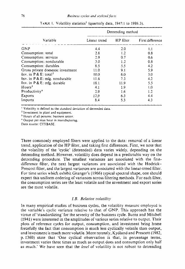
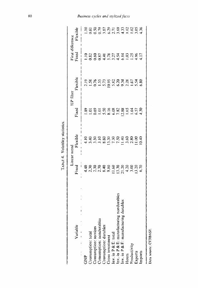
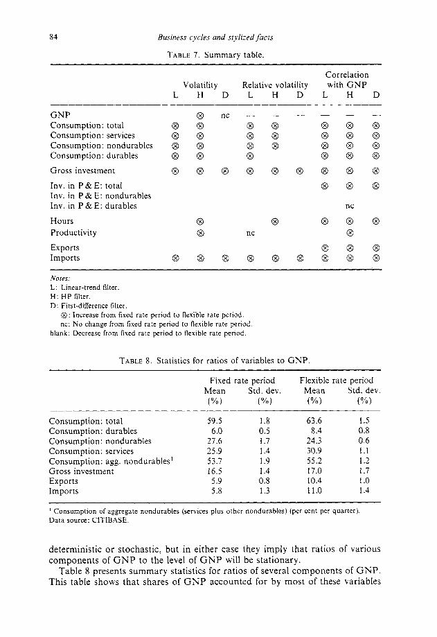
Tables 4 to 6 present business cycle statistics for the fixed and flexible rate periods separately, using the three filters. Table 4 contains volatility statistics, Table 5 contains relative volatility statistics, and Table 6 contains statistics on correlations with GNP. Table 7 summarizes the qualitative results of Tables 4-6, by indicating whether the statistic in question increased, decreased, or did not change between the tixed and flexible-rate periods.
1I.A. Volditj
Table 4 contains results on the cyclic volatility of key macroeconomic aggregates, and details the way in which these statistics changed across the two exchange rate regime periods. We first catalogue the results which are robust to detrending method. Beginning at the bottom of the table, we find that all filters yield the result that the volatility of exports fell in the flexible rate period, while the volatility of imports rose.’ Some surprising (but consistent) results arise for the investment measures. For all detrending methods, we find an increase in the cyclic volatility of gross private domestic investment, yet a decrease in the cyclic volatility of investment in plant and equipment. The difference is due to increases in volatility in components of gross investment not captured in plant and equipment: notably, residential and inventory investment.*
We turn now to results which are not robust to detrending. First, under linear detrending, we find that the volatility of GNP fell slightly in the flexible rate
‘Thl
rLa
4.
Vol
atili
ty
stat
istic
s.
Lin
ear
tren
d IH
P lil
ter
Firs
t di
l‘fe
renc
e V
aria
ble
Fixe
d Fl
exib
le
Fixe
d Fl
exib
le
Fixe
d Fl
exib
le
tr,
E
GN
P 4.
40
4.10
1.
89
2.19
1.
10
1.10
C
onsu
mpt
ion:
to
tal
2.30
3.
40
1.01
1.
58
0.82
0.
81
$’
Con
sum
ptio
n:
serv
ices
2.
30
3.50
0.
69
0.76
0.
60
0.50
2
Con
sum
ptio
n:
nond
urab
les
2.70
3.
10
1.01
1.
55
0.87
0.
79
F C
onsu
mpt
ion:
du
rabl
es
8.40
8.
80
5.50
5.
73
4.41
3.
87
: G
ross
in
vest
men
t 9.
80
13.3
0 X
.16
10.9
5 5.
78
6.29
,”
ln
v.
in
P&E
: to
tal
11.6
0 7.
30
6.08
5.
82
3.27
2.
71
‘Y
; In
v.
in
P &
E:
man
ufac
turi
ng
nond
urab
les
13.3
0 7.
50
7.82
6.
20
4.54
3.
69
2 In
v.
in
P&
E:
man
ufkt
urin
g du
rabl
es
21.2
0 11
.40
12.8
8 9.
34
6.14
4.
33
Hou
rs
4.20
3.
60
1.65
2.
28
I .03
1.
02
$ 2 Pr
oduc
tivity
3.
00
2.80
1.
64
1.67
1.
25
I .02
E
xpor
ts
13.2
0 11
.00
6.57
5.
54
4.96
3.
05
Impo
rts
6.70
10
.40
4.30
6.
80
4.17
4.
36
Dat
a so
urce
: CIT
IBA
SE
.

TA
BLE
5.
Rel
ativ
e vo
latil
ity
stat
istic
s.
Var
iabl
e
GN
P C
onsu
mpt
ion:
to
tal
Con
sum
ptio
n:
serv
ices
C
onsu
mpt
ion:
no
ndur
able
s C
onsu
mpt
ion:
du
rabl
es
Gro
ss
inve
stm
ent
Inv.
in
P&
E:
tota
l ln
v.
in
P&E
: m
anuf
actu
ring
no
ndur
able
s In
v.
in
P &
E:
man
ufac
turi
ng
dura
bles
H
ours
Pr
oduc
tivity
E
xpor
ts
impo
rts
Lin
ear
tren
d Fi
xed
Flex
ible
-.
___ I .
oo
1 .oo
0.
51
0.81
0.
51
0.85
0.
60
0.76
1.
87
2.15
2.
23
3.24
2.58
1.
74
2.96
1.
76
4.70
2.
69
0.93
0.
86
0.67
0.
67
2.93
2.
62
I .49
2.
48
HP
filte
r Fi
rst
diff
eren
ce
Fixe
d Fl
exib
le
Fixe
d Fl
exib
le
1.00
I .
oo
I .oo
I .
oo
0.53
0.
72
0.75
0.
74
0.37
0.
35
0.55
0.
45
s P 0.
53
0.71
0.
79
0.72
$
2.91
2.
62
4.01
3.
52
4.32
5.
00
5.25
5.
72
2
3.22
2.
66
2.97
2.
46
; 4.
14
2.83
4.
13
3.35
6.
81
4.26
5.
58
3.94
g
0.87
1.
04
0.94
0.
93
0.87
0.
76
1.14
0.
93
3.48
2.
53
4.51
2.
77
2.28
3.
11
3.79
3.
96
Dat
a so
urc
e:
CIT
IBA
SE
.

TA
I~L
IZ 6.
Cor
rela
tion
with
G
NP.
Lin
ear
tren
d H
P fi
lter
Firs
t di
tTer
ence
V
aria
ble
Fixe
d Fl
exib
le
Fixe
d Fl
exib
le
Fixe
d Fl
exib
le
____
__
____
_ __
_~~
tu
GN
P 1 .
oo
1.00
1.
00
I .oo
1.
00
1.00
C
onsu
mpt
ion:
to
tal
0.60
0.
93
0.52
0.
82
0.42
0.
60
$.
Con
sum
ptio
n:
serv
ices
0.
54
0.88
0.
56
c 0.
81
0.34
0.
34
Con
sum
ptio
n:
nond
urab
les
0.69
0.
92
0.53
0.
72
0.27
0.
35
,z
Con
sum
ptio
n:
dura
bles
0.
27
0.66
0.
16
2 0.
78
0.31
0.
61
Gro
ss
inve
stm
ent
0.55
0.
80
0.63
;
0.95
0.
72
lnv.
in
P&
E:
tota
l 0.
85
$ 0.
43
0.77
0.
61
0.76
0.
48
0.51
,c
In
v.
in
I’&
E:
man
uktu
ring
no
ndur
;tble
s 0.
27
-0.2
3 0.
49
0.24
0.
25
0.24
2
Inv.
in
P
& E
: m
anuk
tctu
ring
du
rabl
es
;,’
0.77
0.
68
0.67
0.
67
0.43
0.
37
“4
Hou
rs
-0.1
2 -0
.02
0.78
0.
93
0.67
0.
81
Prod
uctiv
ity
0.65
0.
50
0.41
0.
56
0.52
0.
41
2 t:
Exp
orts
-0
.31
0.61
0.
41
0.47
0.
14
0.46
Impo
rts
0.57
0.
87
0.46
0.
85
0.19
0.
54
Dal
a so
urce
: CIT
IDA
SE.

MARIANNE BAXTER 83
period. Yet GNP volatility registers an increase using the HP filter, and is unchanged if the first-difference filter is used. Hours and productivity show modest declines in volatility using the linear-trend and differencing filters, but both register increases in volatility with the HP filter. Looking at consumption, we find that all measures of consumption show increased volatility in the flexible rate period under the linear trend and HP filters, but all show declines with the first-difference filter.
II. B. Relative volatility
As discussed in Section I, relative volatility has interested business cycle researchers at least since the ‘time of Burns and Mitchell. Further, matching relative volatility statistics is a key concern of modern business cycle research as undertaken, for example, by Kydland and Prescott (1982), Hansen (1985), and Prescott (t986). In this subsection, we study a second type of business cycle stylized fact: the volatility of economic aggregates relative to that of GNP.
Table 5 compares relative volatility statistics across the two exchange rate regimes, using the three filters. This table shows that the results for relative volatility are not very different from the results presented in Table 4 for the level of volatility. Specifically, the relative volatility of gross investment, and imports has increased in the flexible rate period; the relative volatilities of plant and equipment investment, productivity, and exports have all decreased. As with levels, relative volatilities of consumption and hours exhibit sensitivity to the detrending method, and nothing conclusive can be said about these variables.
II.C. Comovement with GNP
An important class of business cycle stylized facts involves the comovement of various aggregates with GNP. Table 6 reports the correlations of these variables with GNP by time period and by detrending method. This table contains some of the most robust results that we have found. For all detrending methods, we find that total consumption and each of its components have become more highly correlated with output in the post-1973 period. In addition, the following variables all register increased correlation with output in the post-1973 period: gross investment, total plant and equipment investment, hours, exports, and imports.
For productivity, we find that correlation with GNP increased under the HP filter, and decreased under the other two filters. The correlation of gross investment with GNP increased under all filters, as did the correlation with GNP of total investment in plant and equipment. However, we find that the correlation with GNP of manufacturing durable and nondurable components of plant and equipment investment decreased post-1973. 9 Because the detrending methods remove different trends from each series, this result is surprising but not impossible.
1I.D. Ratios
An important class of macroeconomic models implies that all macroeconomic aggregates (except hours) grow at the same rate: see, for example, the analyses of King et al. (1987), and King ef al. (1988a, b). These common trends may be
84 Businzss cycles and stylized facts
TABLE 7. Summary table.
Volatility Relative volatilitv Correlation with GNP
L H D L H
GNP Consumption: total Consumption: services Consumption: nondurables Consumption: durables
Gross investment
Inv. in P& E: total Inv. in P&E: nondurables Inv. in P&E: durables
Hours
Productivity
Exports Imports
0 0 0 nc
Notes:
L: Linear-trend filter.
H: HP filter.
D: First-difference filter.
Q: Increase from fixed rate period to flexible rate period.
nc: No change from fixed rate period to flexible rate period
blank: Decrease from fixed rate period to flexible rate period.
TABLE 8. Statistics for ratios of variables to GNP.
Fixed rate period Flexible rate period Mean Std. dev. Mean Std. dev.
(“A) W) W) W)
Consumption: total 59.5 1.8 63.6 1.5 Consumption: durables 6.0 0.5 8.4 0.8 Consumption: nondurables 27.6 1.7 24.3 0.6 Consumption: services 25.9 1.4 30.9 1.1 Consumption: agg. nondurables’ 53.7 1.9 55.2 1.2 Gross investment 16.5 1.4 17.0 1.7 Exports 5.9 0.8 10.4 1.0 Imports 5.8 1.3 11.0 1.4
’ Consumption of aggregate nondurables (services plus other nondurables) (per cent per quarter). Data source: CITIBASE.
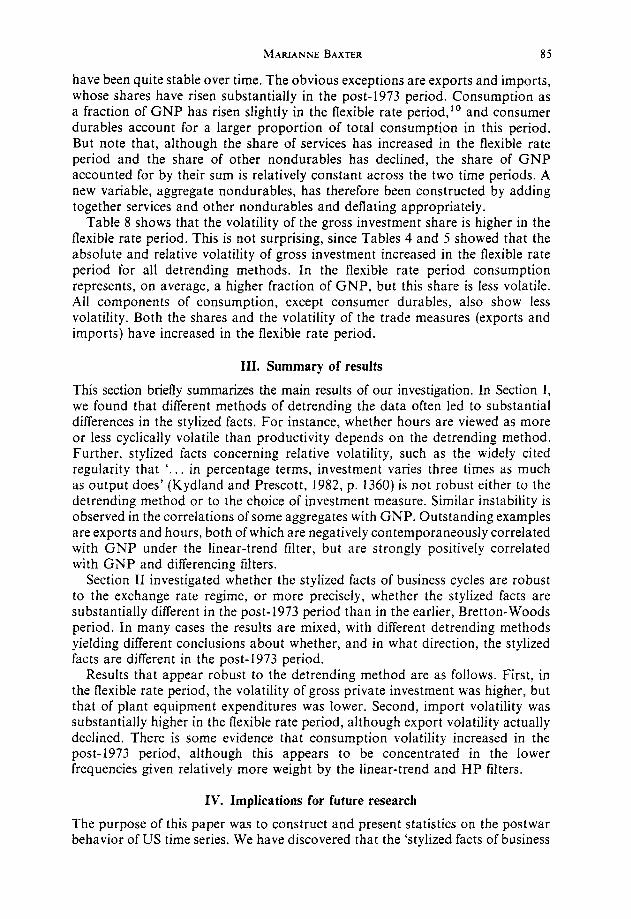
deterministic or stochastic, but in either case they imply that ratios of various components of GNP to the level of GNP will be stationary.
Table 8 presents summary statistics for ratios of several components of GNP. This table shows that shares of GNP accounted for by most of these variables
MARIANNE BAXTER 85
have been quite stable over time. The obvious exceptions are exports and imports, whose shares have risen substantially in the post-1973 period. Consumption as a fraction of GNP has risen slightly in the flexible rate period,” and consumer durables account for a larger proportion of total consumption in this period. But note that, although the share of services has increased in the flexible rate period and the share of other nondurables has declined, the share of GNP accounted for by their sum is relatively constant across the two time periods. A new variable, aggregate nondurables, has therefore been constructed by adding together services and other nondurables and deflating appropriately.
Table 8 shows that the volatility of the gross investment share is higher in the flexible rate period. This is not surprising, since Tables 4 and 5 showed that the absolute and relative volatility of gross investment increased in the flexible rate period for all detrending methods. In the flexible rate period consumption represents, on average, a higher fraction of GNP, but this share is less volatile. All components of consumption, except consumer durables, also show less volatility. Both the shares and the volatility of the trade measures (exports and imports) have increased in the flexible rate period.
III. Summary of results
This section briefly summarizes the main results of our investigation. In Section I, we found that different methods of detrending the data often led to substantial differences in the stylized facts. For instance, whether hours are viewed as more or less cyclically volatile than productivity depends on the detrending method. Further, stylized facts concerning relative volatility, such as the widely cited regularity that ‘. . in percentage terms, investment varies three times as much as output does’ (Kydland and Prescott, 1982, p. 1360) is not robust either to the detrending method or to the choice of investment measure. Similar instability is observed in the correlations of some aggregates with GNP. Outstanding examples are exports and hours, both of which are negatively contemporaneously correlated with GNP under the linear-trend filter, but are strongly positively correlated with GNP and differencing filters.
Section II investigated whether the stylized facts of business cycles are robust to the exchange rate regime, or more precisely, whether the stylized facts are substantially different in the post-1973 period than in the earlier, Bretton-Woods period. In many cases the results are mixed, with different detrending methods yielding different conclusions about whether, and in what direction, the stylized facts are different in the post-1973 period.
Results that appear robust to the detrending method are as follows. First, in the flexible rate period, the volatility of gross private investment was higher, but that of plant equipment expenditures was lower. Second, import volatility was substantially higher in the flexible rate period, although export volatility actually declined. There is some evidence that consumption volatility increased in the post-1973 period, although this appears to be concentrated in the lower frequencies given relatively more weight by the linear-trend and HP filters.
IV. Implications for future research
The purpose of this paper was to construct and present statistics on the postwar behavior of US time series. We have discovered that the ‘stylized facts of business
86 Business cycles and stylized facts
cycles’ are not robust to alternative, commonly-used methods of removing nonstationary components from time series. Further, we have uncovered some evidence of differences across the two postwar exchange rate regimes in the statistical behavior of US macroeconomic aggregates. In this concluding section, we discuss the implications of each of these findings in turn.
ZV.A. Filtering
This paper has documented the extensive dependence of the ‘stylized facts’ on detrending methods. In order to provide a meaningful comparison between the simulated time series of a model economy and the data, it is critical that the same filter be applied to both. But this is not enough, since we have shown that one’s view of the ‘facts’ will be highly colored by the specific filter chosen. Therefore, the researcher should discuss the ways in which (i) the stylized facts of the data and (ii) conclusions about model adequacy would change if another filter were used. Alternatively, he should report enough information about the behavior of the model economy that an interested reader could perform his own sensitivity analysis.
A better solution to the problem of filter-dependence is to let the model itself dictate appropriate treatment of the data. Recently, several researchers have begun to develop unified theories of growth and cycles.” In these models there is no sensible way to separate the data into ‘growth’ and ‘cyclic’ components, since these theories typically have strong cross-frequency restrictions, meaning that shocks to the economic system typically affect both ‘long run growth’ and ‘cyclic fluctuations.’ Further, within a unified theory of growth and cycles, the theory itself will dictate appropriate, stationarity-inducing transformations of the data. The results of the present paper highlight the importance of avoiding an artificial separation of economic time series into ‘growth’ and ‘cycles’ both in modeling and in empirical analyses. The results are simply too sensitive to the way in which this is done.
IV. B. Model dewlopment and econometric evaluation
This paper has documented a number of features of US business cycles, and has catalogued the important ways in which these characteristics differed across the two postwar exchange rate regimes. These characteristics are ones which an empirically relevant theory of the international transmission of business cycles must reproduce. As such, they stand as a challenge to existing theories of cycles and transmission. One particularly interesting set of stylized facts which this study has uncovered is that the correlations between GNP, on the one hand, and consumption, investment, hours, exports, and imports, on the other, all rose in the post-1973 period. This reinforces the Baxter and Stockman (1989) finding that the correlation between consumption and output (measured as industrial production) rose in OECD countries in the flexible rate period. However, Baxter and Stockman found that international output correlations actually declined in the flexible rate period, giving the appearance of increased opportunities for international risk-pooling. This implies that national correlations between output and consumption should also have declined in the flexible rate period. Thus a puzzle remains: why do business cycles look more country-specific in the flexible rate period, which is widely believed to have been characterized by increased
MARIANNE BAXTER 87
openness of financial markets and which has experienced two large, world-wide oil price shocks?
It is tempting to discuss the extent to which one model versus another could potentially explain specific stylized facts which have been uncovered in this analysis. However, it is important not to be seduced into this activity. An empirically relevant model must be able to simultaneously account for many important features of the data. Further, an empirically relevant explanation of these phenomena requires more than a theoretical analysis which shows that these correlations are possible, given as many empirically-unrestricted free parameters as necessary. For example, the Mundell-Fleming model and its modern adaptations predict that fiscal and monetary shocks have different national and international effects, depending on the exchange rate regime in place, and depending on the degree of capital mobility. But can quantitatively- restricted versions of these models simultaneously explain a comprehensive set of the stylized facts laid out in this paper? Similarly, real business cycle models have focused on technological disturbances and fiscal policy shocks as important determinants of the national and international character of business cycles, and quantitatively-restricted versions of these models have had some success in replicating salient features of US business cycles. But an equilibrium business cycle model driven solely by technology shocks cannot explain the consumption/ output puzzle detailed above. Thus it remains for further research to develop fully- specified, quantitatively-restricted models which can simultaneously explain the empirical regularities documented in this paper.
Notes
1. Marston (1985) provides an excellent summary of this literature. 2. Gerlach (1988). on the other hand, used cross-spectral methods to estimate the coherence
between industrial production in OECD countries, and concluded that this measure of international correlatedness of business cycles is higher in the flexible rate period.
3. A notable exception is a recent study by King and Plosser (1989), who apply traditional NBER dating methods to a one-sector equilibrium business cycle model driven by Solow residuals. Interestingly, King and Plosser find that this model can pass the famous ‘test of the Adelman’s.’
4. This graph is adapted from Figure 2 in Singleton (1988). 5. A virtue of using easily-computed statistics such as these is that replication of results and
application to other datasets is straightforward. 6. Indeed, there is nothing about the three filters that suggests that such an ordering should
be preserved for relative volatilities. 7. Although one would like to say whether the changes in volatility discussed here are
statistically significant, serial correlation in the detrended series make conventional F-tests invalid.
8. Space considerations prohibit reporting of moments for these subcomponents of gross investment. These statistics are available from the author, or can be readily computed from the published NIPA data.
9. Expenditures on manufacturing durable plus nondurable plant and equipment represent about half of total plant and equipment expenditures.
10. This is largely due to the fact that consumption as a share of GNP was extremely low during the Korean War.
11. See, for example, King et al. (1988b).

88 Business cycles and stylized facts
References
BAXTER, M., A. STOCKMAN,
of
d
1 l-66.