Business-Cycle Durations and Postwar Stabilization …mwatson/papers/Watson_AER_1994.pdfBusiness-Cycle Durations and Postwar Stabilization of the U.S. Economy ... not relied on the

Business-Cycle Durations and Postwar Stabilization of the U.S. Economy

By MARK W. WATSON*

Average postwar expansions are twice as long as prewar expansions, and contractions are one-half as long. This paper investigates three possible explanations. The first explanation is that shocks to the economy have been smaller in the postwar period. The second explanation is that the composition of output has shifted from very cyclical sectors to less cyclical sectors. The third explanation is that the apparent stabilization is largely spurious and is caused by differences in the way that prewar and postwar business-cycle reference dates were chosen by the NBER. The evidence presented in this paper favors this third explanation. (JEL N10, E32)

A key piece of evidence supporting the efficacy of aggregate-demand management is the observation that, on average, postwar business cycles in the United States have been less severe than in the prewar period. This argument, presented by Arthur Burns (1960) and subsequently investigated by other researchers, has been seriously chal- lenged in a series of papers by Christina Romer (1986a,b, 1989,1991).1 Romer's argument is that the apparent stability of the postwar economy is largely an artifact of

measurement error in the prewar data, which spuriously increases its volatility. However, much of the evidence supporting the contention of postwar stabilization has not relied on the volatility in specific series, but instead on the duration of business cycles calculated using the historical reference dates determined by researchers at the Na- tional Bureau of Economic Research (NBER). These duration data suggest that the average length of recessions has fallen dramatically in the postwar period: during 1854-1929 contractions averaged 20.5 months, while during 1945-1990 they averaged 10.7 months; similarly over the same periods, prewar expansions averaged 25.3 months, while postwar expansions averaged 49.9 months. Francis Diebold and Glenn Rudebusch (1992) show that these prewar- postwar differences are statistically highly significant and robust to many of the changes in NBER business-cycle chronology debated in the historical literature.

This paper investigates three explanations for this apparent stabilization of the postwar economy. The first explanation is that shocks to individual sectors of the economy have been smaller in the postwar period than in the prewar period. This may reflect a fortuitous exogenous change in the process generating shocks, or it may reflect effective government policy dampening the effects of exogenous shocks. The empirical

* Department of Economics, Northwestern Univer- sity, Evanston, IL 60208, and the Federal Reserve Bank of Chicago. This paper is an extension of my discussion of Francis X. Diebold and Glenn D. Rude- busch's (1992) paper, presented at the NBER Eco- nomics Fluctuations meeting in July 1991, and I thank the authors for stimulating my interest in this area. I also thank two referees, Robert Gordon, Robert King, Jeff Miron, Christina Romer, Glenn Rudebusch, and colleagues at the Chicago Federal Reserve Bank for useful comments and suggestions. Special thanks go to Jim Stock for detailed suggestions, to Robert Gordon, Jeff Miron, and Christina Romer for making data available, and to Edwin Denson for excellent research assistance. This work was supported by National Sci- ence Foundation grants SES-89-10601 and SES-91- 22463.

'Also see the papers by Martin N. Bailey (1978), J. Bradford De Long and Lawrence Summers (1986), Victor Zarnowitz and Geoffrey Moore (1986), and Nathan Balke and Robert J. Gordon (1989).

24

VOL. 84 NO. 1 WATSON: BUSINESS-CYCLE DURATIONS AND STABILIZATION 25

analysis reported below offers little support for this explanation.

The second explanation is that the cyclical behavior of individual sectors was the same in the prewar and postwar periods, but that changes in the relative importance of the sectors led to changes in the cyclical behavior of the aggregate economy. For example, the service sector has traditionally been less cyclical than the manufacturing sector and over time has grown in importance relative to the manufacturing sector. Once again, the empirical analysis offered below does not support this explanation.

The third explanation is that the differences in durations are spurious, caused by systematic biases in the information used to form the reference dates. The empirical analysis presented in this paper supports this explanation. In particular, the analysis suggests that the paucity of prewar data forced early NBER researchers to focus their attention on a small number of economic time series, and these series repre- sent sectors of the economy that are systematically more volatile than aggregate activity. This exaggerated volatility was re- flected in longer contractions and shorter expansions in the prewar period.

The remainder of this paper presents evidence on the relative plausibility of these three explanations. In Section I, contraction and expansion durations in "specific cycles" of individual series are investigated to see if these have changed across the prewar and postwar periods. Little evidence of change is found in the individual series. Section II investigates the effect of the changing composition of output on the durations of the business cycle and concludes that this explanation cannot explain the differences between the prewar and postwar durations. Section III reviews the construction of the prewar reference dates and compares the data used to date prewar business cycles with the data used to date postwar cycles. This analysis suggests that the prewar business-cycle chronology relied on data with a much narrower focus than the data used to date postwar cycles. When postwar cycles are dated using data similar to that used to date prewar cycles, little difference

between the prewar and postwar periods is evident. Some concluding comments are offered in the final section.

1. Phase Durations of Specific Series

The questions raised in the Introduction can only be resolved by comparing prewar and postwar data, and as Romer's work shows, extreme care must be exercised in such a comparison: the series used must be of consistent quality (either good or bad) across the prewar and postwar period. Un- fortunately, data availability enforces a trade-off between coverage and sampling interval. The available annual data cover many sectors of the economy but are far from ideal for business-cycle analysis, since annual data can mask short or mild contractions. Monthly data are more useful, but there are few monthly series of consistent quality spanning a significant portion of the prewar and postwar period. Moreover, for both the monthly and annual data the requirement that the data be consistently measured in the prewar and postwar period means that series subject to large structural changes (new products, etc.) are necessar- ily omitted from the analysis. With these limitations noted, this section uses available monthly and annual data to uncover prewar-postwar changes in the average phase durations of "specific cycles" associ- ated with these series.

Identifying specific cycles in economic time series requires precise definitions of a "contraction" and an "expansion." Unfor- tunately, the definition of contraction and expansion used by the NBER is too vague for this purpose.2 This paper uses an objec-

2Burns and Wesley Mitchell (1946) give the official definition of contractions and expansions. These are phases of the business cycle, which they defined as follows: Business cycles are a type of fluctuation found in the, aggregate economic activity of nations that organize their work mainly in business enterprises: a cycle con- sists of expansions occurring at about the same time in many economic activities, followed by similarly general recessions, contractions, and revivals which merge into the expansion phase of the next cycle; this sequence of changes is recurrent but not periodic; in duration business cycles vary from more than one year to ten or

26 THE AMERICAN ECONOMIC REVIEW MARCH 1994

tive definition embedded in an algorithm developed by Gerhard Bry and Charlotte Boschan (1973).3 This algorithm is a set of ad hoc filters and rules that determine business-cycle turning points in an economic time series. Essentially, the algorithm isolates local minima and maxima in a time series, subject to constraints on both the length and amplitude of expansions and contractions. For many series, the Bry- Boschan algorithm does a remarkably good job at reproducing the turning points selected by "experts." For example, Figure 1 shows monthly values of the logarithm of pig-iron production from 1877 to 1929. The horizontal lines on the graph are the turning points selected by the Bry-Boschan procedure; the arrows point to the turning points selected by Burns and Mitchell (1946).4 Little difference between the Bry- Boschan and Burns-Mitchell peaks and troughs is evident.

Consistent with practice at the NBER, the Bry-Boschan algorithm dates contractions and expansions using the level (or log level) of the series, rather than the detrended series. Thus, contractions correspond to sequences of absolute declines in a series, and not to periods of slow growth relative to trend. In business-cycle jargon, the algorithm dates "business cycles" and not "growth cycles." This will be important when interpreting the changes in prewar and postwar average phase durations for series that experienced a significant change

in their trend rate of growth. Changes in trend rates of growth have obvious effects on contraction and expansion lengths: decreases in average growth rates lead to increases in average contraction duration and decreases in average expansion duration.

Table 1 shows average phase durations calculated using the Bry-Boschan dating algorithm for a variety of monthly prewar and postwar series. For many of these series the prewar and postwar data are not perfectly comparable, and comparisons using a variety of postwar series are presented. To eliminate any effect of the Great Depres- sion, the prewar period is truncated in 1929, although the substantive conclusions offered below are unaltered if the period is extended to 1940. For each series the table presents the average length of contractions (C), and the average length of expansions (E) in the prewar and postwar period. As discussed above, since contractions are defined as absolute declines, rather than declines below trend growth, average annual growth rates (X = sample mean of [log(xt) - log(xt 12)]) over the two sample periods are shown, as are the t statistics for testing the null hypothesis of no change in the growth rate (tq). In addition, the standard deviation of the annual growth rates (or) for the prewar and postwar periods are shown. Finally, following Diebold and Rudebusch (1992), the table presents the Wilcoxon rank-sum statistic (Wc and WE) for comparing the prewar and postwar contraction and expansion phase durations. The statistic is presented in standardized form and can be interpreted like a t statistic for a significant change in the average duration.5 (For example, absolute values greater than 2 are statistically significant.)

A serious problem with the monthly data is that there are few direct indicators of

twelve years; they are not divisible into shorter cycles of similar character with amplitude approximating their own. [p. 3] A more recent statement of the official definition of a recession offered by the NBER (1992) is only slightly more specific: ... a recession is a recurring period of decline in total output, income, employment, and trade, usually lasting from six months to a year, and marked by widespread contractions in many sectors of the economy. Historically, phases for specific series and business-cycle reference dates have been determined judgmentally.

3 rhe Bry and Boschan programs are described and applied in a novel and interesting way by Robert King and Charles Plosser (1989).

4The Burns and Mitchell (1946) dates are from their chart 53 (p. 373).

5See E. L. Lehmann (1975) for a general discussion of the statistic. The standardized form of the statistic shown in the table is asymptotically standard normal. (Its exact sampling distribution can also be deduced.) In large samples, a standard t test can also be used to compare the average durations. For the data considered here, the results using a standard t test are similar to the results using the W statistics.


LCD

CD

o

O-1 : I Il IWI I I I I II-

CD ~ ~ ~ ~ ~ ~ ~ ~ Dt

FIGURE 1. PIG-IRON PRODUCTION: BRY-BOSCHAN AND BURNS-MITCHELL PEAKS AND TROUGHS

Key: Solid lines are Bry-Boschan peak dates; dashed lines are Bry-Boschan trough dates. Arrows denote Burns- Mitchell peak and trough dates.

output or employment, since many of the series are from the financial sector and are imperfect indicators of sectoral or aggregate output. The first panel of the table shows results for a variety of financial series. In summary, real stock prices show little change in cyclical behavior, long-term interest rates show a slight increase in the length of postwar expansions with little change in the length of contractions, and commercial paper rates show a decrease in postwar contraction duration and increase in expansion duration.6 For these series the only statisti-

cally significant change is for commercial paper expansions. The other financial series -business failures, stock-exchange volume, and bank clearings-show large changes in trend growth rates, which makes it difficult to compare the prewar and postwar average durations.

Panel B presents results for production indicators. The first set of comparisons involves prewar pig-iron production and postwar industrial production indexes for metals and steel. In the postwar period, contractions are longer and expansions shorter, but this reduction is undoubtedly related to the decline in the growth rate of this sector. The next comparison involves prewar railroad freight ton-miles and postwar manufacturers' shipments. Again, the rapid

6Matthew Shapiro (1988) examines prewar and postwar stock price volatility and finds no significant difference between the periods.


TABLE 1-AVERAGE PHASE DURATIONS, MONTHLY DATA

Series Sample period X u C E tX WC WE

A. Financial Markets:

RR stock index 1860:1-1929:12 1.67 14.73 20.1 25.9 S&P industrials 1947:1-1990:12 3.49 16.14 17.9 25.4 -0.5 0.1 -0.4 S&P transportation 1970:1-1990:12 1.97 21.70 21.3 29.0 0.2 -0.3 -0.3

S&P composite 1871:1-1929:12 1.79 15.19 18.0 24.9 S&P composite 1947:1-1990:12 3.08 15.67 17.3 25.9 -0.4 -0.2 -0.5

Dow Jones Industrials 1897:1-1929:12 4.07 20.85 17.8 22.8 Dow Jones Industrials 1947:1-1990:12 2.20 16.04 21.2 26.7 0.4 0.5 -1.3

Business failures 1894:1-1929:12 0.40 49.73 29.3 30.9 Business failures 1948:1-1990:9 8.85 44.76 15.9 27.6 -0.9 2.4 0.3

NYSE volume 1875:1-1929:12 5.75 52.06 19.1 19.1 NYSE volume 1947:1-1990:12 11.79 28.91 15.0 37.1 -0.7 0.9 -1.5

RR bond yields 1857:1-1929:12 -0.05 1.76 18.5 22.6 Corporate bond yields (AAA) 1947:1-1990:12 0.16 0.97 21.9 29.3 -0.8 -0.9 -0.0 Industrial bond yields (AAA) 1947:1-1990:12 0.16 0.93 21.0 30.3 -0.8 -0.6 -0.4 Corporate bond yields (BAA) 1947:1-1990:12 0.17 1.09 24.5 28.0 -0.8 -1.6 -0.5 Industrial bond yields (BAA) 1947:1-1990:12 0.18 1.04 22.4 30.7 -0.9 - 1.0 -0.8

Commercial paper rate 1857:1-1929:12 -0.04 0.34 28.9 25.0 Commercial paper rate 1947:1-1990:12 0.16 1.91 18.1 34.8 -0.6 1.5 -2.0

Bank clearings 1875:1-1929:12 3.56 7.25 13.4 24.9 Bank clearings 1970:1-1990:12 8.93 6.69 13.0 117.0 -2.4 -0.8 -1.9

B. Production Indicators:

Pig-iron production 1877:1-1929:12 6.08 30.78 12.9 28.0 IP metals 1947:1-1990:12 1.01 20.16 18.9 22.9 0.9 -1.7 0.8 IP iron and steel 1947:1-1990:12 0.17 27.14 19.8 23.4 0.9 -1.7 0.8

growth in the prewar period makes this comparison difficult. The potentially most informative comparison involves the prewar industrial production index constructed in Jeffrey Miron and Romer (1990) and postwar industrial production indexes. Compar- ing the Miron-Romer series to the postwar aggregate index of industrial production yields results very similar to the NBER phase durations for expansions: postwar expansions are roughly twice as long as prewar expansions. While this comparison is tempting, it is inappropriate because the mix of goods in the Miron-Romer series differs significantly from the mix of goods in the aggregate industrial production (IP) index. To control for the mix of goods in the index, the final row of the table compares the Miron-Romer index to a postwar index

with approximately the same product mix.7 This postwar index has cyclical properties remarkably close to the prewar Miron-

7This postwar index is a weighted average of industrial production indexes for metals, mining, food, apparel products, and rubber and plastics. It is fully described in the Data Appendix. The Miron-Romer index for the prewar period is composed primarily of "materials," while the aggregate postwar IP index is composed of both materials and "products." Materials account for approximately 40 percent of postwar IP, and products account for the remaining 60 percent. The materials and product components have markedly different average phase durations in the postwar period: the materials component of industrial production has average contraction and expansion durations of 14.8 months and 31.1 months, respectively; the corresponding values for the products component are 14.7 months and 57.7 months.

VOL. 84 NO. 1 WATSON: BUSINESS- CYCLE DURATIONS AND STABILIZATION 29

TABLE 1- Continued.

Series Sample period X r C E tx WC WE

RR freight ton-miles 1866:8-1929:12 6.60 10.48 12.2 39.0 Manufacturers' shipments 1947:1-1990:12 2.29 6.89 14.3 34.1 2.5 - 1.0 0.3

IP-Miron/Romer 1884:1-1929:12 4.53 16.59 10.8 23.0 IP-FRB 1947:1-1990:12 3.65 6.26 13.7 58.6 0.3 -1.7 -2.6 IP-Miron/Romer

(approximate) 1947:1-1990:12 1.76 10.01 13.5 22.4 0.9 -0.8 0.3

IP- 1899 value-added weights 1947:1-1990:12 2.21 5.76 14.1 31.8 IP- 1977 value-added weights 1947:1-1990:12 3.04 6.72 13.7 36.9 -0.6 0.4 -0.2

C. Foreign Trade:

Exports 1866:7-1929:12 4.37 19.90 13.4 27.9 Exports 1977:1-1990:12 2.89 11.38 20.3 29.3 0.3 -0.4 -0.5

Imports 1866:7-1929:12 3.85 21.07 17.3 32.9 Imports 1977:1-1990:12 3.31 9.46 20.0 32.0 -0.1 -0.6 0.3

D. Other Indicators:

Wholesale prices 1890:1-1929:12 1.36 11.65 17.5 28.1 Producer prices 1947:1-1990:12 3.52 4.92 13.9 59.8 - 1.1 1.0 -0.8

Plans for new buildings 1868:1-1929:12 5.63 73.66 16.6 19.1 Building permits 1947:1-1990:12 -0.21 26.52 18.0 19.8 0.7 -0.7 -0.5

Notes: E and C respectively denote average lengths of expansions and contractions (in months), X denotes the average annual growth rate in the series, a denotes the standard deviation of the annual growth rate, and tx is the (autocorrelation-robust) t statistic for testing equality of growth rates across the two time periods. Wc and WE are the standardized Wilcoxon rank-sum statistics for comparing the prewar and postwar durations of contractions and expansions, respectively. Expansions and contractions were determined by the Bry-Boschan algorithm using the logarithms of the series, except for interest rates where levels were used. IP denotes an index of industrial production.

Romer index.8 The final entries in panel B will be discussed in Section II.

Panel C compares the prewar-postwar cyclical durations of imports and exports. Both imports and exports are much less volatile in the postwar period, but there is little apparent change in average phase durations. Finally, panel D contains two com-

8Romer (1992) carries out the "flip-side" of this experiment. She adjusts the prewar Miron-Romer index so that it is comparable with the postwar Federal Reserve Board (FRB) index. Using this adjusted series, she finds that from 1887 to 1917 contractions averaged 9.7 months, and expansions averaged 32.2 months. These results suggest that the average lengths of prewar and postwar contractions are roughly equal, but that prewar expansions are considerably shorter than postwar expansions.

Unfortunately, Romer's adjustment procedure is not perfect, and this makes her results difficult to interpret. Her procedure is as follows. After appropriate adjust-

ment for trends and seasonals, the logarithm of the FRB industrial-production index is regressed on six leads and lags of the logarithm of the Miron-Romer index over the period 1923-1928. This regression (again, with appropriate treatment of trends and seasonals) is used to backcast the FRB aggregate IP index from the Miron-Romer index. The potential problem with this procedure is that it ignores the regression error and so can potentially produce a backcasted series with different cyclical properties than the true index.

To investigate this possibility, I replicated Romer's procedure using the postwar FRB index and my postwar approximation to the Miron-Romer index. I regressed the log of the FRB index on a constant, a time trend, and six leads and lags of the log of the approximate Miron-Romer index over the period 1947-1990. The fitted value from this regression is a postwar analogue of the backcast IP series used by Romer. During the postwar period, these fitted values had average contraction lengths of 12.2 months and average expansion lengths of 32.2 months. The corresponding values for the FRB index over the same period were 14.1 and 58.3 months. Thus, for the postwar period at least, the procedure produces average expansion lengths that have a substantial negative bias.


TABLE 2-AVERAGE PHASE DURATIONS, ANNUAL SERIES

A. Aggregate Series: Begin-1929 1946-end

Series Begin End X C E X r C E tx Wc WE

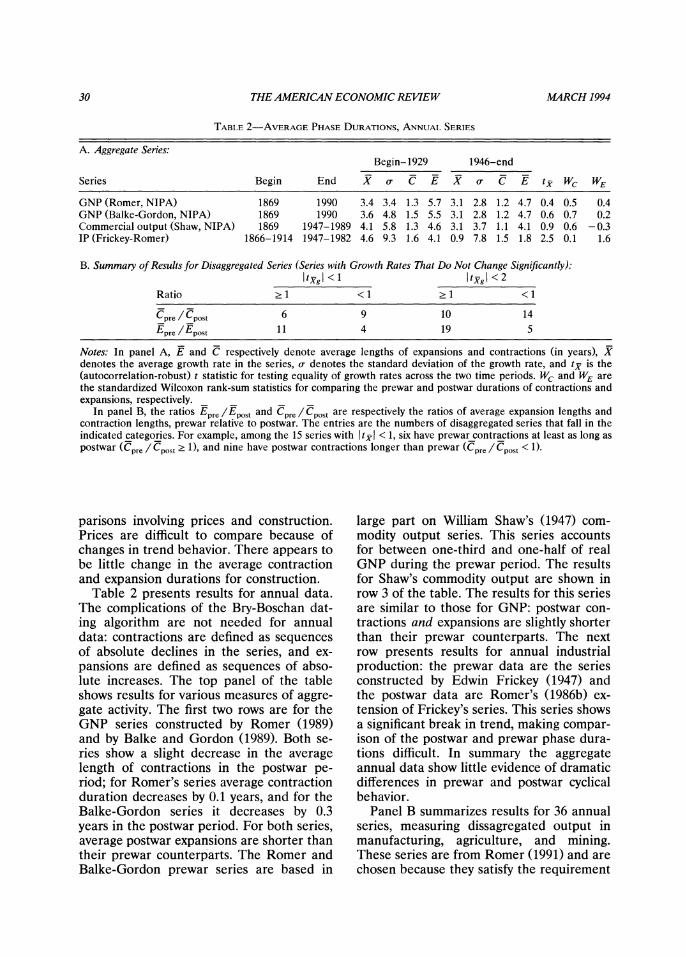
GNP (Romer, NIPA) 1869 1990 3.4 3.4 1.3 5.7 3.1 2.8 1.2 4.7 0.4 0.5 0.4 GNP (Balke-Gordon, NIPA) 1869 1990 3.6 4.8 1.5 5.5 3.1 2.8 1.2 4.7 0.6 0.7 0.2 Commercial output (Shaw, NIPA) 1869 1947-1989 4.1 5.8 1.3 4.6 3.1 3.7 1.1 4.1 0.9 0.6 -0.3 IP (Frickey-Romer) 1866-1914 1947-1982 4.6 9.3 1.6 4.1 0.9 7.8 1.5 1.8 2.5 0.1 1.6

B. Summary of Results for Disaggregated Series (Series with Growth Rates That Do Not Change Significantly): I t'Y' < 1 tyg I < 2

Ratio ?1 <1 ?1 <1

Cpre / Cpost 6 9 10 14 Epre /Epost 11 4 19 5

Notes: In panel A, E and C respectively denote average lengths of expansions and contractions (in years), X denotes the average growth rate in the series, o- denotes the standard deviation of the growth rate, and tx is the (autocorrelation-robust) t statistic for testing equality of growth rates across the two time periods. Wc and WE are the standardized Wilcoxon rank-sum statistics for comparing the prewar and postwar durations of contractions and expansions, respectively.

In panel B, the ratios Epre/Epost and Cpre/Cpost are respectively the ratios of average expansion lengths and contraction lengths, prewar relative to postwar. The entries are the numbers of disaggregated series that fall in the indicated categories. For example, among the 15 series with I tyj < 1, six have prewar contractions at least as long as postwar (Cpre / Cpost ? 1), and nine have postwar contractions longer than prewar (Cpre / Cpost < 1).

parisons involving prices and construction. Prices are difficult to compare because of changes in trend behavior. There appears to be little change in the average contraction and expansion durations for construction.

Table 2 presents results for annual data. The complications of the Bry-Boschan dating algorithm are not needed for annual data: contractions are defined as sequences of absolute declines in the series, and expansions are defined as sequences of absolute increases. The top panel of the table shows results for various measures of aggregate activity. The first two rows are for the GNP series constructed by Romer (1989) and by Balke and Gordon (1989). Both series show a slight decrease in the average length of contractions in the postwar period; for Romer's series average contraction duration decreases by 0.1 years, and for the Balke-Gordon series it decreases by 0.3 years in the postwar period. For both series, average postwar expansions are shorter than their prewar counterparts. The Romer and Balke-Gordon prewar series are based in

large part on William Shaw's (1947) commodity output series. This series accounts for between one-third and one-half of real GNP during the prewar period. The results for Shaw's commodity output are shown in row 3 of the table. The results for this series are similar to those for GNP: postwar contractions and expansions are slightly shorter than their prewar counterparts. The next row presents results for annual industrial production: the prewar data are the series constructed by Edwin Frickey (1947) and the postwar data are Romer's (1986b) extension of Frickey's series. This series shows a significant break in trend, making comparison of the postwar and prewar phase durations difficult. In summary the aggregate annual data show little evidence of dramatic differences in prewar and postwar cyclical behavior.

Panel B summarizes results for 36 annual series, measuring dissagregated output in manufacturing, agriculture, and mining. These series are from Romer (1991) and are chosen because they satisfy the requirement

VOL. 84 NO. 1 WATSON: BUSINESS-CYCLE DURA TIONS AND STABILIZATION 31

of consistent quality through the entire sample period.9 Detailed results for these series are presented in an earlier version of this paper (Watson, 1992); panel B summarizes the key findings. Of the 36 series, 24 showed no significant change in trend, in the sense that the t statistic for a trend break was less than 2 in absolute value; 15 of the series had a t statistic less than 1 in absolute value. Panel B shows the ratio of average prewar to postwar contraction and expansion durations for these series. The results are striking: for the majority of the series, postwar contractions tend to be longer, and postwar expansions tend to be shorter than their prewar counterparts.

Taken together, the annual data provide little support for the notion that contractions are shorter and expansions longer in the postwar period. An important caveat is that, while this may accurately reflect the cyclical behavior of these series, it may also reflect the limitations of using annual data to analyze phase durations.

Three conclusions emerge from these data. First, they suggest that there has been little change in the average phase durations of sectoral output. This is evident from the annual data, in which many sectors were considered, and in the monthly data, which considered pig-iron production and a fixed-weight index of industrial production. The second conclusion is that these results carry over to aggregate series also. This is evident from the annual data on GNP and unemployment and the monthly data on stock prices. Third, while average phase durations do not seem to have changed, there is evidence that volatility has decreased. Many of the disaggregated series used to construct panel B of Table 2 show a significant decrease in variance for the postwar period. A reduction in variability can also be seen for many of the monthly series.

These conclusions are tempered by three caveats: first, the monthly data are very limited; second, the annual sectoral data repre-

sent production of commodities, and there are no data on the other sectors of the economy; finally, the prewar annual GNP series are less representative of the aggregate economy than the postwar series because of measurement problems docu- mented in Balke and Gordon (1989) and Romer (1989).

IL. Sectoral Changes

One potential explanation for the reduced cyclicality in the postwar period is the changing composition of aggregate output. This explanation is discussed in some detail in Zarnowitz and Moore (1986), who document the increasing importance of "less cyclical" relative to "more cyclical" sectors in the postwar period. Clear evidence for the importance of composition is evident in Table 1. For the postwar period, the FRB industrial-production index and the (approximate) Miron-Romer index differ only in their composition and yet have significantly different cyclical behavior. The FRB index of industrial production is an index of the output of 252 sectors in manufacturing, mining, and utilities, each weighted by its value-added. The approximate Miron- Romer index, described in detail in the Data Appendix, is a weighted average of five sub- aggregates of industrial production, chosen to mimic the composition of the prewar index of industrial production constructed in Miron and Romer (1990).

The dramatic difference in the cyclical behavior of the postwar indexes suggests that, if the composition of output in the Miron-Romer index is representative of the composition of output during the prewar period, then the data provide strong support for the sectoral-composition explanation of postwar duration stabilization. How- ever, as pointed out by Romer (1992 p. 20), the Miron-Romer index is not representative of the composition of prewar output: "... . it is based on many fewer series than is the modern FRB index, and many sectors are either over- or under-represented relative to their actual value added." Thus, the differences in the FRB index and the postwar (approximate) Miron-Romer index do

91 thank Christina Romer for supplying me with these data.


not accurately reflect the changes in the composition of output between the prewar and postwar period.

However, indexes that do reflect the typi- cal prewar and postwar composition of the industrial sector can be constructed. Table 1 shows aggregate indexes of industrial production (manufacturing plus mining) constructed from postwar data using value- added weights from the 1899 and 1977 Censuses. The series were constructed from the same sectoral indexes and differ only in the weights used to form the aggregated index. (The construction of the series is described in detail in the Data Appendix.) While the value-added weights changed significantly from 1899 to 1977, these changes had little effect on the average phase durations of the composite indexes. The changes in the sectoral composition of industrial production that have occurred over the 20th century appear to have had little effect on the length of expansions and contractions.10

This discussion of industrial output is somewhat beside the point, however. The major sectoral shift discussed by Zarnowitz and Moore (1986) and others is not a shift within the industrial sector, but rather the shift from the industrial sector to less cyclical sectors like services and government. Some evidence on the potential importance of this kind of sectoral change is presented

in Table 3. This table shows the historical evolution of sectoral shares of total employment, together with postwar average phase durations of sectoral employment. During the postwar period, the more cyclical sectors-manufacturing; transportation, communications and public utilities; and mining -grew more slowly than the less cyclical sectors. Most notable is the share of manufacturing (a highly cyclical industry) which fell from 34.7 percent of nonagricultural employment in 1948 to 17.3 percent in 1990, and the share of service employment (a very noncyclical sector), which rose from 11.5 percent in 1948 to 25.6 percent in 1990. This increase in the share of employment in noncyclical sectors suggests a reduction in the cyclicality of aggregate employment, even in the absence of changes in the individual sectors.

However, a closer examination of the table suggests that sectoral changes may not explain the differences between the prewar and postwar periods. In particular, the table shows that growth rates within sectors have changed significantly through time. For example, manufacturing employment grew at an average rate of 2.7 percent from 1869 to 1929, and only 0.4 percent from 1948 to 1990. Since downturns are measured as absolute declines, and not as declines relative to trend, this suggests that manufacturing was less cyclical in the prewar period (when it had a larger trend) than in the postwar period (when it had a smaller trend). Thus, even though manufacturing accounted for a smaller share of aggregate employment in the postwar period, it may have been more cyclical. Overall, the trends in sectoral employment paint an ambiguous picture of aggregate cyclicality in the prewar and postwar data.

If monthly prewar employment data were available, it would be possible to model changes in the stochastic processes govern- ing sectoral employment across the prewar and postwar periods and to deduce implica- tions for the changing cyclical properties of aggregate employment. Unfortunately, the only reliable prewar sectoral employment data are from the decennial census. These data can be used to estimate trends, but by

10There is evidence that higher-frequency changes in composition affect phase durations. The aggregate FRB index, which is constructed using time-varying value-added weights, has average expansions that are 12 months longer than the corresponding 1977-fixed- weight index. The FRB index uses value-added weights that change every five years and so represents the evolving composition of industrial output. It should not be surprising that an index constructed using time- varying value-added weights has longer expansions than a fixed-weight index, because relative value-added co- varies positively with relative quantities. This implies, for example, that during expansions relative value- added increases for industries whose output rises more than average. Thus, an index with time-varying weights will tend to increase more than a fixed-weight index during an expansion and will tend to decrease less during a contraction. This will lead to series with a higher mean growth rate, longer average expansions, and shorter average contractions.

VOL. 84 NO. 1 WATSON: BUSINESS-CYCLE DURATIONSAND STABILIZATION 33

TABLE 3-AVERAGE PHASES, SHARES, AND GROWTH RATES FOR NONAGRICULTURAL EMPLOYMENT

Average growth rate 1947-1990 Share of total employment (percentage)

Series C E 1869 1929 1948K 1948 1990 1869-1929 1947-1990

Total employment 11.7 54.8 100.0 100.0 100.0 100.0 100.0 3.0 2.1 Manufacturing 17.4 31.8 34.4 28.4 30.7 34.7 17.3 2.7 0.4 Services - 21.7 17.8 15.1 11.5 25.6 2.7 4.0 Trade 10.8 89.2 15.2 21.5 22.7 20.7 23.7 3.6 2.7 Transportation, com-

munications, and public utilities 13.8 30.8 9.9 11.0 8.5 9.3 5.3 3.2 0.8

Construction 15.9 45.9 9.5 6.4 6.6 4.9 4.7 2.4 2.2 Government 17.0 192.5 6.0 7.8 10.5 12.6 16.6 3.5 2.7 Mining 31.9 33.6 2.5 2.8 2.0 2.2 0.7 3.2 -0.5 F.I.R.E. - 0.8 4.3 3.8 4.0 6.2 5.8 3.2

Notes: E and C respectively denote average lengths of expansions and contractions (in months). The shares for 1869, 1929, and 1948K are from John Kendrick's (1961 p. 308) table A-VII. Data for 1947-1990 are from the BLS establishment survey. F.I.R.E. denotes finance, insurance, and real estate.

themselves they provide little information about the cyclical properties of the series. This makes it impossible to identify all of the prewar-postwar changes in the sectoral employment processes that affect the cyclicality in aggregate employment.

Using the prewar dicennial census data and the postwar monthly data, however, it is possible to conduct some experiments to investigate the plausiblity that sectoral shifts are largely responsible for the changing average phase durations. The first experiment focuses on the trends in the sectoral employment and asks whether these trends per se can explain the differences in the prewar-postwar average phase durations. Another set of experiments is used to see whether other plausible changes in the stochastic process can explain the apparent postwar duration stabilization.

The first experiment is carried out as follows. First, for each sector, models for the trend are estimated for both the prewar and postwar periods. The prewar trend model is estimated using the decennial census data, and the postwar trend model is estimated using monthly data available from the BLS Establishment Survey. The postwar monthly data are then detrended, and the resulting series is used to estimate a model for the short-run variability and covariability of the sectoral data. This short-run model is

then appended to the estimated prewar model for the trends to produce a model for the prewar monthly data. Thus, the prewar and postwar models differ only in their im- plications for the trend behavior of the data; they share the same model for shorter-run movements in the data. The cyclical properties of the resulting employment series from the prewar and postwar models can then be deduced.

The results from implementing this procedure are shown in Table 4. The trends for each sector are estimated by regressing the logs of the data on a constant and time trend. The prewar regressions used decennial data from 1869-1929, and the postwar regressions used monthly data from 1948- 1990.11 In both cases the short-run model was estimated as a VAR(4) using the detrended logarithms of the monthly postwar data. The resulting prewar and postwar models were then used to generate pseudo- monthly employment data for the 1869-1929 and 1948-1990 periods, the Bry-Boschan algorithm was used to date business cycles in the resulting sectoral and aggregate em-

1"In an earlier version of this paper (Watson, 1992), results were also presented for trends estimated by allowing for kinks in the trend line every 20 years. The results were very similar to those presented in Table 4.


TABLE 4-AVERAGE PHASES FOR DATA GENERATED

BY THE TREND-VAR MODEL

Prewar Postwar

Series X C E X C E

Total employment 3.1 11.9 74.6 2.2 13.3 55.9

Manufacturing 2.9 14.3 37.4 0.6 19.2 23.5 Services 2.7 10.3 226.4 4.1 Trade 3.6 10.2 198.1 2.6 11.7 107.1 Transportation, communications,

and public utilities 3.4 11.9 91.4 0.8 18.7 29.0 Construction 2.3 16.2 31.8 1.9 17.0 28.9 Government 3.5 12.6 185.9 3.0 12.7 127.2 Mining 3.3 19.0 40.9 -0.4 26.3 25.8 F.I.R.E. 6.1 - - 3.2

NBER reference dates - 21.2 26.5 10.7 49.9 (1.00) (0.00) (0.15) (0.42)

Notes: X denotes the actual average annual rate of the sector. E and C respectively denote average lengths of expansions and contractions (in months) calculated from the simulated data. The values for the NBER reference dates are the actual average phase durations computed using the reference dates. The values in parentheses are the percentiles of empirical distribution of the simulated data that correspond to the NBER average phase durations.

ployment data, and average contraction and expansion lengths were calculated for the realizations. This procedure was repeated 500 times, and the resulting average phase durations are reported in the table.

Two conclusions follow from the table. First, the generated aggregate postwar data have average phase durations very similar to the actual postwar aggregate employment data, and these in turn are similar to the average phase durations of NBER-dated business cycles. Thus, the Gaussian VAR model mimics the cyclical properties of the postwar data. Second, the generated prewar aggregate data have average contraction lengths similar to the postwar data and average expansion lengths more than one year longer than the postwar data. This suggests that the underlying trend behavior in the sectoral employment data would be expected to lead to less cyclical behavior in the prewar period than in the postwar period. The explanation for this result can be found in the sectoral data. Cyclical sectors such as manufacturing, mining, and transportation had larger growth rates in the prewar period and were consequently less

cyclical. This feature carries over to the aggregate employment series.

These conclusions are reinforced by percentiles of the empirical distributions from the 500 replications corresponding to the prewar and postwar NBER-dated business cycles. These percentiles are shown in parentheses in Table 4 below the average phase durations for the NBER reference dates. For example, looking at the postwar phase durations, 15 percent of the realizations from the postwar model had average contraction lengths less than 10.7 months (the average duration of NBER-dated postwar contractions), and 42 percent of the realizations had average expansion lengths shorter than 49.9 months (the average duration of postwar NBER-dated expansions). On the other hand, 100 percent of the realizations from the prewar model had contractions that were shorter than the average duration of the NBER-dated prewar contractions, and there were no realizations with expansions shorter than the average duration of NBER-dated prewar expansions. These percentiles indicate that the average phase durations for the postwar


NBER-dated business cycles are consistent with the trend-VAR model used to generate the data but that the prewar NBER- dated business cycles are not consistent with the model.

The second set of experiments focuses on other characteristics of the sectoral-employment stochastic process that can potentially explain the differences in the prewar and postwar phase durations. For example, shocks may have been more highly corre- lated across sectors in the prewar period. This would tend to increase the variance in the aggregate employment series and potentially make it more cyclical.12 Alternatively, sectoral employment may have been more volatile in the prewar period. Unfortu- nately, since high-frequency prewar employment data are not available, it is impossible to investigate these potential explanations statistically. However, it is possible to experiment with modifications of the model char- acterizing the postwar data (e.g., doubling the correlation between the shocks) to find out what kinds of modifications are required to explain the prewar phase durations.

While the VAR(4) fits the data well, it is not well suited for these experiments because it allows complicated dynamic interaction among the eight sectors. This makes it difficult to isolate the characteristics of the process which are responsible for the phase durations. Instead of using the VAR, the experiments are carried out using the dynamic factor model:

( 1) xi = axift + ut

(2) ft = Olft-1 + 02ft-2+ et

(3) u =pu1 +8El (3 t =Pit -1 +?

where x< is the detrended level of logarithm employment in the ith sector at time t, ft is a scalar "common factor," et and E' are zero-mean white-noise processes with vari- ances oe2 and o-E2, respectively, and E(et?i )

=E(et?) = 0 for all i, t, , and i j. In this model, all of the dynamic interaction in the sectors comes through the common factor ft. The "uniquenesses," ut, are uncorre- lated across sectors and allow each sector to move independently of the other sectors.

This model was fit to the detrended postwar data, and the results are shown in Table 5A.13 The results look sensible. The most cyclical sectors (mining, construction, and manufacturing) have the largest values of a, indicating the largest amount of covariation. The least cyclical sectors (government, services, and finance, insurance, and real estate [F.I.R.E.]) have the smallest values of a. The common factor, ft, and each of the uniquenesses ut, are highly persistent with exact or near unit autoregressive roots.14

Pseudo-prewar and postwar data were generated by appending the dynamic factor model onto the models for the prewar and postwar trends. The results from 500 realizations of the processes are shown in the first two rows of Table 5B. This model produces data with average contraction lengths similar to the trend-VAR model, but with somewhat longer average expansions. The standard deviation of growth rates of the simulated series are also shown. The differences in trend rates across the series and across periods lead to a slightly larger standard deviation in the prewar period.

12Steve Davis suggested this potential explanation.

13Here the flexible trends specified in footnote 11 were used. In particular, in the prewar period kinks in the trend were allowed in 1889 and 1909, and in the postwar period a kink was allowed in 1968:1. Again, as in the VAR model, similar results are found if single trends are estimated for the prewar and postwar periods.

14 Diagnostic tests, checking the statistical adequacy of the model, are not presented. Undoubtedly, these tests would suggest that the model is too restrictive and is not an adequate statistical description of the postwar data. This should not be too troubling: the purpose of the estimated model is not to test a null hypothesis or to construct forecasts, circumstances in which the mis- specification could be very important. Rather, the estimated model is to serve as a benchmark for some experiments that will give some rough answers to questions about the prewar and postwar data. A careful analysis of these and related postwar data using dynamic factor models is contained in Edwin Denson (1993).


TABLE 5-DYNAMIC FACTOR MODEL

A. Estimated Model: aui =p F, + u,

Ft = OlFtIl + 02It2 + e, Var(e,) = 1.0

Sector a (r p

Manufacturing 0.0030 0.0044 0.97 Services 0.0006 0.0018 0.99 Trade 0.0012 0.0018 0.99 Transportation, communication, and public utilities 0.0016 0.0051 0.94 Construction 0.0029 0.0120 0.96 Government 0.0002 0.0036 1.00 Mining 0.0027 0.0179 0.99 F.I.R.E. 0.0004 0.0017 1.00

X = 1.788 02 = -0.797

B. Average Phases for Data Generated by the Trend-Dynamic Factor Model:

Data C E

Parameters from Estimated Model: Generated data, prewar trends 11.8 (0.99) 81.8 (0.00) 4.4 Generated data, postwar trends 12.2 (0.29) 63.8 (0.26) 3.6

Prewar Results Using Modified Parameters:

ai multiplied by v2, ori2 reduced 13.2 (0.99) 51.9 (0.00) 5.6

ai multiplied by V 13.2 (0.99) 52.0 (0.01) 5.7 ai multiplied by 3 16.4 (0.97) 31.4 (0.16) 11.2 ai multiplied by 5 18.0 (0.90) 26.6 (0.53) 18.0

Notes: In panel A, x, denotes the deviations of the logarithms of the data from trend. The trend is of the form A0 + AIt + A2t[I(t > r)], where 1F is the indicator function and r is 1967:12. The model was estimated using data from 1947:1-1990:12. The restriction Var(e,) = 1 is a normalization that serves to identify the ai. In panel B, the numbers in parentheses are the percentiles of the empirical distribution corresponding to the NBER average phase durations. In the first row of "prewar results" in panel B, o-i2 is reduced by a?, so that the variance of x, is unchanged.

The remaining rows of the table show results for modifications of the dynamic factor model. For example, in the third row of Table 5B, the model was modified by multi- plying each of the factor loadings by C2 and reducing the variance of the uniquenesses by an offsetting amount. (A proportional increase in the factor loadings is observa- tionally equivalent to increasing the standard deviation of the common factor.) This doubles the correlation between the sectors while leaving the variance of each sector unchanged. This modification lengthens average contractions and shortens average expansions, but not nearly enough to explain

the prewar NBER data. In the next three rows the factor loadings are increased by varying amounts, and the uniqueness vari- ances are unaltered. The results suggest that a dramatic increase in the covariance of the sectors is necessary to explain the results: the factor loadings need to be increased by a factor of 5, which corresponds to an increase in the covariance of the sectors by a factor of 25. This modification has a dramatic effect on the variability of the data: the standard deviation of the annual growth rate in the aggregate pseudo-prewar data is five times larger than that for the postwar data.


This section suggests two conclusions about the effect of changes in the composition of employment on prewar and postwar cyclicality. First, differences in the trend rate of growth across sectors do not explain the differences in the prewar and postwar average phase durations. Second, very dramatic, and implausibly large changes in the covariance structure of the prewar and postwar employment data are necessary to explain the prewar average phase durations.

III. Biases in the Prewar Data

The results from Sections I and II, suggest that there is little in the data to support the claim that the postwar period has wit- nessed a reduction in the duration of cyclical contractions and an increase in the duration of cyclical expansions. Why is such a change evident in the NBER business-cycle chronology? One explanation is that NBER researchers chose the prewar reference dates in a way that fundamentally differed from the way that the postwar reference dates were chosen. Two possibilities suggest themselves. First, the relatively paucity of prewar data suggests that NBER researchers may have chosen reference dates for the prewar period using data that were systematically more cyclically volatile than the aggregate economy, and as more data became available, this defect was corrected in the postwar period. This would imply that the apparent postwar stabilization is due to the changing composition of series used to date the cycle; it is not due to changes in the cyclical behavior of individual series or to changes in the composition of aggregate output or employment. The second possibility is that the prewar data may have been processed differently than the postwar data. For example, the prewar data may have been detrended while the postwar data were not.

To investigate the merits of these possibilities it is useful to review the procedure that NBER researchers used to determine the prewar reference dates.15 The prewar

chronology was chosen judgmentally, based on both quantitative and qualitative information. The qualitative information con- sisted in large part of the "business annals" collected in Willard Thrope (1926). These annals are a summary of contemporaneous reports that appeared in the business and popular press; for the United States they cover the period 1790-1925. The Thorpe annals provided an initial set of reference dates, which were then refined by examining available monthly, quarterly, and annual time series.

The quantity and quality of these data improved dramatically over the sample period covered. For example, only 19 monthly or quarterly series were available in 1860; eight of these were price series, eight were financial variables, and only three were related to production: hog receipts in Chicago, cattle receipts in Chicago, and shoe shipments from Boston. By 1930 the availability of data had changed dramatically: 710 monthly and quarterly series were available, and 245 of these related to production and personal incomes.16 Aggregate employment and production indexes played no role in the dating of the early cycles. Monthly data on aggregate nonagricultural employment did not become available until 1929, although an index of factory employment extended back to 1914 (Burns and Mitchell, 1946 p. 74). The earliest monthly index of industrial production used by Burns and Mitchell extended back to 1904.17 Monthly and quarterly estimates of personal income and gross and net national product did not exist for the pre-1920 period. Burns and Mitchell (1946 table 21) list 46 monthly and quarterly series available before 1890. Of these, ten are indirect indicators of business activity, such as the volume of bank clear-

15The most complete and detailed discussion of the

procedures is given in Burns and Mitchell (1946). De- tailed and thorough reviews of the procedure can be found in Moore and Zarnowitz (1986), Diebold and Rudebusch (1992), and Romer (1992).

16These data are from table 17 and footnote 24 (p. 81) in Burns and Mitchell (1946).

17This was Babson's index of the physical volume of business (see Burns and Mitchell, 1946 p. 73).


ings, four are orders for durable goods or construction, two are production indicators, 15 are price indexes or price series, nine are financial indicators such as stock prices and interest rates, and four are indicators of business failures. Many of these series were included in the monthly indicators included in Table 1.

Unfortunately the historical record does not provide a detailed description of how Thorpe's qualitative data were combined with the available statistical data to determine the prewar reference dates. Romer (1992) provides a very useful summary of the historical record. She has traced the pre-1927 reference dates back to an NBER news bulletin dated March 1, 1929, which was apparently written by Mitchell, but the document contains little specific guidance about how the dates were determined. On the other hand, Mitchell's 1927 book, Busi- ness Cycles: The Problem and Its Setting, contains a detailed discussion of Thorpe's annals and the available statistical data that could potentially be used for choosing reference dates.

Romer (1992) points out that two time series, the A.T.T. business index and Sny- der's clearing index, receive particular attention in the discussion in Mitchell's 1927 book. The A.T.T. index begins in 1877, and is a combination of data series meant to measure general business activity. From 1877 to 1884 it was based solely on pig-iron production; bank clearing outside New York City and blast-furnace capacity were added in 1885, and wholesale prices were added in 1892 (Mitchell, 1927 p. 294). Snyder's clearing index begins in 1875 and is based on bank clearings outside New York City, deflated by a price index. As stressed by Romer, the key characteristic of both of these series is that they are presented as deviations from trends, rather than levels. Thus, if these series influenced the choice of prewar dates, they could impart a "growth-cycle" bias in the prewar business- cycle chronology.

From the available historical record, it is impossible to determine exactly what role the A.T.T. index and Snyder's index played in determining the NBER's prewar refer-

ence dates and the consequent growth-cycle bias imparted to average phase durations. However, it is possible to estimate the mag- nitude of any potential bias. This can be done by comparing the average phase durations for the levels and detrended values of the two most important components of the A.T.T. business index and Snyder's clearing index: pig-iron production and bank clearings. If there are large differences between the average phase durations for the levels and the detrended values, then there may be a large growth-cycle bias in the NBER's prewar phase durations, at least to the ex- tent that Burns and Mitchel (1946) relied on the A.T.T. and Snyder index. If the average phase durations for the levels and detrended series are similar, then any potential growth-cycle bias is small.

The average prewar phase durations for the levels and detrended values of pig-iron production and bank clearings are given in Table 6. As expected, the detrended series have longer average contractions and shorter average expansions than the levels. How- ever, the differences are not large. For pig- iron production, the difference is 2.4 months for contractions and 4.9 months for expansions. For detrended bank clearings, contractions are 2.8 months shorter, and expansions are 6.1 months longer, than the levels series. To put these differences into per- spective, recall that the postwar contractions are an average of 9.8 months shorter than prewar contractions, and postwar expansions are an average of 24.6 months longer than prewar expansions. Thus, while the use of the detrended A.T.T. business index and Snyder's clearing index may have biased the average phase durations, these biases are small compared to differences in the prewar and postwar average phase du-

18 rations.?

18Romer (1992) carries out a similar exercise using the Miron-Romer IP series over the 1884-1927 period and a dating algorithm similar to the Bry-Boschan algorithm. She finds that contractions are 3.2 months longer and expansions are 3.4 months shorter, using the detrended data.

VOL. 84 NO. 1 WATSON: BUSINESS-CYCLE DURATIONSAND STABILIZATION 39

TABLE 6-COMPARISON OF PREWAR AVERAGE PHASE DURATIONS

FOR LEVELS AND DETRENDED SERIES

Series Sample period C E

Pig-iron production, levels 1877:1-1929:12 12.9 28.0 Pig-iron production, detrended 1877:1-1929:12 15.3 23.1

Bank clearings, levels 1875:1-1929:12 13.4 25.0 Bank clearings, detrended 1875:1-1929:12 16.2 18.9

Notes: The detrended series are the exponentiated residuals from an ordinary least- squares regression of the logarithm of the series onto a constant and linear trend.

An alternative explanation of the differences in the average prewar and postwar durations is that the data used to date the prewar cycles were systematically more volatile than aggregate activity and that this bias was eliminated in the postwar period. A simple way to investigate this explanation is to date postwar business cycles using only those indicators that were used to date the prewar cycles, that is, to "Romerize" the postwar reference dates by artificially re- stricting the postwar data to be as limited as the prewar data.

Table 7 presents peak and trough dates for seven series covering the same range of activities as the 46 series available to Burns and Mitchell. The notable deletions from the list is any consideration of bank clearing and prices, because of the change in the drift in these series shown in Table 1. More- over, I have not attempted to construct postwar annals analogous to those constructed by Thorpe.19

Evident in Table 7 is a clustering of "specific cycles" for the individual series, consistent with the notion of the business cycle. While the Bry-Boschan algorithm de- termines turning points in individual series, it does not solve the multivariate problem of determining a "reference cycle" from a col-

lection of series. Here, I have used judgment based on the turning points in the individual series to construct a set of reference dates. These are shown in the table along with the NBER reference dates. In selecting the reference dates, I assumed that the two production indexes were coincident indicators; that is, on average, they moved contemporaneously with the cycle. When specific cycles in these series approximately coincided, I averaged the peak and trough dates. For each production index there were specific cycles that did not correspond with movements in other series, and these were ignored when choosing the reference dates. Table 8 shows the reference dates that I selected along with the lead-lag relations of the individual indicators. These suggest rea- sonable conformity across cycles.20

These pseudo-reference dates suggest a much more volatile postwar period than the NBER reference dates. They suggest three more recessions (1951:4-1952: 1, 1966: 1- 1967:6, and 1984:4-1986: 1), longer con-

19My impression from reading the business press during the 1980's and 1990's is that postwar annals would greatly overstate the cyclical variability of the economy.

20 An alternative approach to determining the refer-

ence dates is to extract a single factor from a dynamic factor model estimated using these data series. Turning points in this extracted factor could then be determined by the Bry-Boschan program. I experimented with this approach but found it unsatisfactory. The results from the procedure depend critically on the variance of the factor relative to its average drift. Unfortunately, this ratio is econometrically unidenti- fied in a factor model and must be determined judgmentally. I chose instead to apply judgment to the turning-point data directly.

TABLE

7-PEAK

AND

TROUGH

DATES,

SELECTED

SERIES

Approximate

industrial production,

Industrial

Stock

prices

Miron-Romer

production,

Building

(S&P

com-

Commercial

Pseudo-

(less

steel)

iron

and

steel

permits

posite

index)

paper

rate

Exports

Imports

reference

NBER

Peak

Trough

Peak

Trough

Peak

Trough

Peak

Trough

Peak

Trough

Peak

Trough

Peak

Trough

Peak

Trough

Peak

Trough

1948:6

1949:10

1948:10

1949:10

1947:10

1949:1

1949:6

1949:7

1950:7

1948:8

1949:10

1948:11

1949:10

1951:1

1951:7

1951:6

1952:7

1950:7

1951:7

1951:4

1952:1

1953:7

1953:12

1953:7

1954:4

1952:11

1953:9

1953:1

1953:9

1953:8

1954:12

1953:7

1954:2

1953:7

1954:5

1957:3

1958:4

1955:9

1958:4

1955:2

1958:2

1956:7

1957:12

1957:10

1958:7

1956:6

1958:4

1957:8

1958:4

1960:4

1961:1

1959:6

1962:6

1958:11

1960:12

1959:7

1960:10

1960:1

1961:7

1959:11

1961:9

1960:4

1961:2

1961:12

1962:6

1964:2

1965:4

1966:10

1967:6

1966:1

1966:11

1966:1

1966:10

1966:12

1967:6

1966:10

1967:6

1969:11

1970:7

1969:11

1971:8

1969:2

1970:1

1968:12

1970:7

1969:12

1972:2

1969:11

1971:1

1969:12

1970:11

1973:9

1975:3

1973:12

1975:7

1972:12

1975:3

1973:1

1974:12

1974:7

1976:12

1973:10

1975:5

1973:11

1975:3

1978:7

1979:7

1978:11

1980:7

1977:8

1980:4

1976:9

1980:4

1977:11

1978:9

1980:1

1980:1

1980:7

1981:7

1982:12

1981:2

1982:12

1980:9

1981:10

1980:11

1982:7

1981:5

1983:1

1980:4

1983:5

1980:2

1983:3

1981:4

1982:12

1981:7

1982:11

1984:6

1985:1

1984:2

1987:1

1984:2

1984:10

1983:6

1984:7

1984:7

1986:10

1985:1

1986:7

1984:7

1985:3

1984:4

1986:1

1986:1

1986:9

1986:4

1988:1

1987:8

1989:11

1989:1

1989:12

1988:10

1989:3

1989:10

1990:4

1989:3

1990:6

1989:6

1990:7

Notes:

For

the

individual

series,

peaks

and

troughs

were

determined

by

the

Bry-Boschan

algorithm.

The

column

labeled

"pseudo-reference" is a

set of

reference

dates

chosen

from

the

peak

and

trough

dates of

the

individual

series.

The

column

labeled

"NBER"

contains

the

NBER

peak

and

trough

dates.

VOL. 84 NO. 1 WA TSON: BUSINESS-CYCLE DURA TIONS AND STABILIZATION 41

TABLE 8-SPECIFIC CYCLE LEADS AND LAGS RELATIVE TO REFERENCE CYCLE

Approximate Industrial Stock prices Pseudo- Miron-Romer production, Building (S&P com- Commercial reference (less steel) iron and steel permits posite index) paper rate Exports Imports

Peak Trough Peak Trough Peak Trough Peak Trough Peak Trough Peak Trough Peak Trough Peak Trough

1948:8 1949:10 -2 0 2 0 -10 -9 -4 11 9

1951:4 1952:1 -3 -6 2 6 -9 -6

1953:7 1954:2 0 -2 0 2 -8 -5 -6 -5 1 10

1956:6 1958:4 9 0 -9 0 -16 -2 1 -4

1959:11 1961:9 5 -8 -5 9 -12 -9 -4 -11 2 -2

1966:10 1967:6 0 0 -9 -7 -9 -8 2 0

1969:11 1971:1 0 -6 0 7 -9 -12 -11 -6 1 13

1973:10 1975:5 -1 -2 2 2 -10 -2 -9 -5 9 19

1978:9 1980:1 -2 -6 2 6 -13 3 -24 3

1981:4 1982:12 3 0 -2 0 -7 -14 -5 -5 1 1 -12 5 14 3

1984:4 1986:1 2 -12 -2 12 -2 -15 -10 -18 3 9 9 -6 3 -10

1989:6 5 -5 -8 -22 -3 4 -3

Average: 1.2 -3.2 -1.2 3.4 -8.7 -6 -7.7 -4.8 1.5 4.1 0.3 2.8 -3.5 1.8

Notes: Table entries are the difference between the peak and trough dates of the specific series and the corresponding pseudo-reference dates.

TABLE 9-AVERAGE PHASE LENGTHS FROM NBER AND PSEUDO-REFERENCE DATES

Dates C E Wc WE

Prewar (NBER) 20.5 25.3 Postwar (NBER) 10.7 49.9 2.83 -2.62 Postwar (pseudo-

reference) 15.6 28.9 0.67 -0.17

Notes: E and C respectively denote average lengths of expansions and contractions (in months). Wc and WE are the standardized Wilcoxon rank-sum statistics for comparing the prewar and postwar contractions and durations, respectively.

tractions, and shorter expansions.21 Sum- mary statistics comparing average phase durations from these pseudo-reference dates to the NBER prewar and postwar chronologies are presented in Table 9. These data suggest little change in the length of expan-

sions across the prewar and postwar periods and a reduction in the length of contractions that is only half as great as suggested by the NBER chronology. Moreover, nei- ther of the changes is statistically significant.

IV. Concluding Remarks

This paper has investigated three explanations for the postwar duration stability evident in the NBER business-cycle chronology. Little support is found for explanations that lead to duration stability across individual sectors of the economy: for most individual series, average contraction and expansion durations for the prewar and postwar periods are similar. The data also cast doubt on the changing composition of output and employment as the cause of the apparent postwar stability. Historical differences in trend growth rates of sectoral employment explain little of the observed changes in average duration. An explanation that is consistent with the data is that the prewar NBER business-cycle chronology was determined by data that, at least in the postwar period, are systematically more

21 Each of these periods corresponded to a marked slowdown in economic activity as measured by the NBER experimental coincident index. These slow- downs were not severe enough to be regarded as recessions.


TABLE A1-NBER BCD NUMBERS FOR MONTHLY SERIES

Monthly series NBER BCD ID number

Pig-iron production M01585 Railroad stock prices M11032/M04008 NYSE volume M11006 Bank clearings M12051/M04008 linked

to M12052/M04008 in 1919 Business failures M09144/M04008 RR bond yields M13024 Commercial paper M13111 Building plans M02245/M04008 linked

to M02246/M04008 in 1899:2 RR ton-miles M03032 linked to M03033

in 1922:12 Wholesale price index M04010 linked to M04011

in 1914:12 Total exports M07007/M04008 Total imports M07068/M04088

volatile than the aggregate economy. Thus, selection bias in the data series available to researchers in the prewar period appears to be the most likely explanation for the postwar duration stability apparent in the NBER data.

Two points should be kept in mind when interpreting these conclusions. First, even though the evidence supports the view that the average lengths of prewar and postwar expansions and contractions are not significantly different, the data summarized in Ta- bles 1 and 2 suggest a decrease in volatility, at least for many of the series studied. Thus, while business-cycle durations have re- mained constant, there is evidence that their amplitude has decreased. The second point is that these results should not be viewed as a criticism of the work summarized in Burns and Mitchell (1946). These authors were careful to point out the limitations of their reference dates.22 Their primary interest was not in the reference dates and the lengths of cycles, but in how individual series moved over the cycle. No analysis has been offered in this paper to address the robustness of their finding in this regard to changes in the prewar chronology.

This research challenges the reliability of the prewar reference dates relative to their postwar counterparts and questions the quality of statistics, like average phase durations, based on the prewar reference dates. The challenge for economic historians is to develop statistical corrections for the selection bias that affects statistics constructed from the prewar reference dates or, better yet, to use additional data and improved methods to determine more accurately the dates themselves.

DATA APPENDIX

This appendix describes the prewar and postwar data used in the paper. All of the postwar data, unless otherwise noted, are from Citibase. All of the prewar data, unless otherwise noted, are from the NBER Business-Cycle Database (BCD).

Prewar Data

Annual Data.-The sources for annual data are given in the tables and the text.

Monthly Data.-The NBER BCD numbers for the monthly series used are given in Table Al. The S&P and Dow Jones nominal stock prices are from Moore (1961). They were deflated by the NBER BCD series M04008 (an index of the general price level). The prewar monthly industrial series is from Miron and Romer (1990).

Transformations. -Many of the series required some preprocessing. In most cases this was to correct obvious

22See, in particular Chapter 4 of Burns and Mitchell (1946).


coding errors in the NBER Business Cycle Database. The specific transformations were:

M01585: 10 was subtracted from the observation in 1880:11; observations in 1926:1, 1928:1, and 1930:1 were multipled by 10.

M11032: Missing values in 1872:4 and 1914:8-1914:11 were estimated by linear interpolation.

M13024: Missing values during 1857:9-1857:10 were estimated by linear interpolation.

M02246: Missing values in 1929:3:9-1929:4 were estimated by linear interpolation; The series was then seasonally adjusted using the RATS exponential moving-average procedure.

Miron and Romer industrial production and M03033: These series were seasonally adjusted using the RATS exponential moving-average procedure.

M07068: A missing value in 1867:12 was estimated by linear interpolation.

Postwar Data

Annual Data.-The sources for annual data are given in the tables and the text.

Monthly Data.-The Citibase labels for the monthly series used are given in Table A2. For bank clearings, debits (demand deposits) at other than New York banks is from the Federal Reserve Bulletin. The nominal values were deflated by the CPI (Citibase series PUNEW).

The Postwar Approximation to the Miron-Romer In- dex of Industrial Production.-The approximate Miron- Romer IP series for the postwar period is calculated as

IPMR = [(wmet)(ipdm2) + (wmin)(ipmin)

+ (wfood)(ipnfo2) + (wapp)(ipnt3)

+ (wrub)(ipnch5)]/ w

where:

wmet = 31.91 + 2.13

wfood = 2.53+5.42+7.76+9.28+2.18

wmin = 9.92 + 2.54 + 3.85

wapp = 11.89 + 4.62

wrub = 5.97

w = wmet + wfood + wmin + wrub + wapp

with the variables defined as follows:

wmet: the composite weight in Miron and Romer given to (i) pig-iron capacity and (ii) tin imports;

wfood: the composite weight in Miron and Romer given to (i) sugar meltings at four ports, (ii) cattle receipts in Chicago, (iii) hog receipts in Chicago, (iv) Minneapolis flour shipments, and (v) coffee imports;

wmin: the composite weight in Miron and Romer given to (i) anthracite coal shipments, (ii) Connellsville coke shipments, and (iii) crude petroleum products, Appalachian Region;

wapp: the composite weight in Miron and Romer given to (i) wood receipts at Boston and (ii) raw silk imports;

wrub: the composite weight in Miron and Romer given to crude rubber imports.

Postwar Fixed-Weight Indexes of Industrial Produc- tion.-The postwar fixed-weight indexes were constructed as weighted averages of 16 subaggregated IP indexes: ipmin, ipnfo2, ipnfo5, iptexap, iplumf, ipnpr2, ipnpr3, ipnch4, ipnch5, inpt4, ipdcl2, ipmet, ipmach, ipdt, and ipdetc, where

iptexap = (wl)[ipnt2(t)] + (w2)[ipnt3(t)] is an index for textiles plus apparel;

iplumf = (w1)[ipdcl3(t)]+ (w2)[ipdf2(t)] is an index for lumber plus furniture;

ipmet = (wl)[ipdm2(t)]+(w2)[ipdm5(t)J is an index for metals;

ipmach = (wl) [ipdma3(t)] + (w2) [ipdma4(t)] + (w3)[ipdi(t)] is an index for machinery plus instruments; and where the weights (wl, etc.) are chosen to add to 1 and are determined from the 1977 value-added weights given in table A.1 of Industrial Production (1986 Edition). The weights used to form the 1977 weighted average index are also given in this table.

The 1899 weights are from two sources. Historical Statistics of the United States (1975 p. 239) shows value-added in manufacturing and mining for 1899. Solomon Fabricant (1940 pp. 635-39) gives value- added in different sectors of manufacturing. Fabri- cant's categories do not perfectly match those in the FRB index, and they were assigned as follows: food + beverages (ipnfo2); tobacco products (ipnfo5); textile products (iptexap); forest products (iplumf); paper products (ipnpr2); printing and publishing (ipnpr3); chemical products (ipnch2); petroleum and coal products (ipnch4); rubber products (ipnch5); leather products (ipnt4); stone, clay, and glass (ipdc12); iron and steel (ipmet); machinery (ipmach); transportation equipment, (ipdt); miscellaneous products (ipdetc).

Transformations.-Series were adjusted as follows:

LPTU: An outlier in 1983:8 was replaced with a lin- early interpolated value.

LPMI: To adjust for outliers, first the trend was re- moved from the logarithm of the series using a Hodrick-Prescott filter. Second, extreme observations (greater than three standard deviations) were set equal to the mean. Finally, this adjusted series was then added to Hodrick-Prescott trend, and the series was exponentiated.

F6TED and F6TEM: These series were seasonally adjusted using the RATS exponential moving-average procedure.


TABLE A2-CITIBASE LABELS FOR MONTHLY SERIES

Description Citibase label

Industrial production IP Industrial production, materials IPM Industrial production, products IPP Industrial production, mining IPMIN Industrial production, metals IPDM2 Industrial production, iron and steel IPDM3 Industrial production, clay, glass, stone products IPDCL2 Industrial production, lumber and products IPDCL3 Industrial production, miscellaneous durable manufacturers IPDETC Industrial production, furniture and fixtures IPDF2 Industrial production, instruments IPDI Industrial production, transportation equipment IPDT Industrial production, fabricated metal products IPDM5 Industrial production, nonelectrical machinery IPDMA3 Industrial production, electrical machinery IPDMA4 Industrial production, foods IPNF02 Industrial production, tobacco products IPNF05 Industrial production, textile mill products IPNT2 Industrial production, apparel products IPNT3 Industrial production, leather and products IPNT4 Industrial production, paper and products IPNPR2 Industrial production, printing and publishing IPNPR3 Industrial production, chemicals and products IPNCH2 Industrial production, rubber and plastics products IPNCH5 Industrial production, petroleum products IPNCH4 Consumer price index PUNEW Manufacturers' shipments MFGS/PUNEW Exports F6TED/PUNEW Imports F6TMD/PUNEW S&P industrials FSPIN/PUNEW S&P transportation FSPTR/PUNEW S&P composite FSPCOM/PUNEW Dow Jones Industrials FSDJ/PUNEW NYSE volume FSVOL Corporate bond yield (AAA) FYAAAC Industrial bond yield (AAA) FYAAAI Corporate bond yield (BAA) FYBAAC Industrial bond yield (BAA) FYBAAI Commercial paper rate FYCP Business failures FAIL Producer prices PW Building permits HSBP Total nonagricultural employment LPNAG Construction employment LPCC Manufacturing employment LPEM F.I.R.E. employment LPFR Mining employment LPMI Government employment LPGOV Service employment LPS Wholesale and retail trade employment LPT Transportation and public-utilities employment LPTU


FSPCOM, FSDJ, FSPIN, FSPTR, FAIL, DDOB, F6TED, and F6TMD: These series were all deflated by PUNEW.

REFERENCES

Bailey, Martin N. "Stabilization Policy and Private Economic Behavior." Brookings Papers on Economic Activity, 1978, (1), pp. 11-50.

Balke, Nathan S. and Gordon, Robert J. "The Estimation of Prewar Gross National Product: Methodology and New Evi- dence." Journal of Political Economy, February, 1989, 97(1), pp. 38-92.

Bry, Gerhard and Boschan, Charlotte. Cyclical analysis of time series: Selected procedures and computer program. New York: Columbia University Press, 1971.

Burns, Arthur F. "Progress Towards Eco- nomic Stability." American Economic Re- view, March 1960, 50(1), pp. 1-19.

Burns, Arthur F. and Mitchell, Wesley C. Mea- suring business cycles. New York: National Bureau of Economic Research, 1947.

De Long, J. Bradford and Summers, Lawrence H. "The Changing Cyclical Variability of Economic Activity in the United States," in Robert J. Gordon, ed., The American business cycle: Continuity and change. Chicago: University of Chicago Press, 1986, pp. 679-734.

Denson, Edwin, M. "An Analysis of Postwar Output, Employment, and Productivity." Unpublished manuscript, Northwestern University, 1993.

Diebold, Francis X. and Rudebusch, Glenn D. "Have Postwar Economic Fluctuations Been Stabilized?" American Economic Review, September 1992, 82(4), pp. 993-1005.

Fabricant, Solomon. The output of manufacturing industries, 1899-1937. Kingsport, TN: Kingsport Press, 1940.

Frickey, Edwin. Production in the United States, 1860-1914. Cambridge, MA: Har- vard University Press, 1947.

Historical statistics of the United States, colonial times to 1970. U.S. Department. of Com- merce, Washington, DC: U.S Govern- ment Printing Office, 1975.

Industrial production. Washington, DC: Board of Governors of the Federal Reserve Sys- tem, 1986.

Kendrick, John W. Productivity trends in the United States. Princeton, NJ: Princeton University Press, 1961.

King, Robert G. and Plosser, Charles I. "Real Business Cycles and the Test of the Adel- mans." Unpublished manuscript, Univer- sity of Rochester, 1989.

Lehmann, E. L. Nonparametrics. San Fran- cisco, CA: Holden Day, 1975.

Miron, Jeffrey A. and Romer, Christina D. "A New Monthly Index of Industrial Produc- tion, 1884-1940." Journal of Economic History, June 1990, 50(2), pp. 321-37.

Mitchell, Wesley C. Business cycles: The problem and its setting. New York: National Bureau of Economic Research, 1927.

Moore, Geoffrey H. Business cycle indicators. Princeton, NJ: Princeton University Press, 1961.

Moore, Geoffrey H. and Zarnowitz, Victor. "The Development and Role of the NBER's Business Cycle Chronologies," in Robert J. Gordon, ed., The American business cycle: Continuity and change. Chicago: University of Chicago Press, 1986, pp. 735-79.

National Bureau of Economic Research. "Re- cessions." Release by the NBER's Public Information Office, 1992.

Romer, Christina D. "Spurious Volatility in Historical Unemployment Data." Journal of Political Economy, February 1986a, 94(1), pp. 1-37.

. "Is the Stabilization of the Postwar Economy a Figment of the Data?" Amer- ican Economic Review, June 1986, 76(3), pp. 314-34.

. "The Prewar Business Cycle Re- considered: New Estimates of Gross Na- tional Product, 1869-1908." Journal of Political Economy, February 1989, 97(1), pp. 1-37.

_. "The Cyclical Behavior of Individ- ual Production Series, 1889-1894." Quar- terly Journal of Economics, February 1991, 106(1), pp. 1-32.

. "Remeasuring Business Cycles: A Critique of the Prewar NBER Reference

46 THE AMERICAN ECONOMIC REV7EW MA4RCH 1994

Dates." National Bureau of Economic Research (Cambridge, MA) Working Pa- per No. 4150, 1992.

Shapiro, Matthew D. "The Stabilization of the U.S. Economy: Evidence from the Stock Market." American Economic Review, December 1988, 78(5), pp. 1067-79.

Shaw, William H. The value of commodity output since 1869. New York: National Bureau of Economic Research, 1947.

Thorpe, Willard L. Business annals. New York: National Bureau of Economic Re-

search, 1926. Watson, Mark W. "Business Cycle Durations

and Postwar Stabilization of the U.S. Economy." National Bureau of Economic Research (Cambridge, MA) Working Pa- per No. 4005, 1992.

Zarnowitz, Victor and Moore, Geoffrey H. "Major Changes in Cyclical Behavior," in Robert J. Gordon, ed., The American business cycle: Continuity and change. Chicago: University of Chicago Press, 1986, pp. 519-72.

Documents

Business-Cycle Durations and Postwar Stabilization …mwatson/papers/Watson_AER_1994.pdfBusiness-Cycle Durations and Postwar Stabilization of the U.S. Economy ... not relied on the