Bursty and Hierarchical Structure in Streams ∗

Jon Kleinberg †

Abstract

A fundamental problem in text data mining is to extract meaningful structure

from document streams that arrive continuously over time. E-mail and news articles

are two natural examples of such streams, each characterized by topics that appear,

grow in intensity for a period of time, and then fade away. The published literature

in a particular research field can be seen to exhibit similar phenomena over a much

longer time scale. Underlying much of the text mining work in this area is the following

intuitive premise — that the appearance of a topic in a document stream is signaled

by a “burst of activity,” with certain features rising sharply in frequency as the topic

emerges.

The goal of the present work is to develop a formal approach for modeling such

“bursts,” in such a way that they can be robustly and efficiently identified, and can

provide an organizational framework for analyzing the underlying content. The ap-

proach is based on modeling the stream using an infinite-state automaton, in which

bursts appear naturally as state transitions; it can be viewed as drawing an analogy

with models from queueing theory for bursty network traffic. The resulting algorithms

are highly efficient, and yield a nested representation of the set of bursts that imposes

a hierarchical structure on the overall stream. Experiments with e-mail and research

paper archives suggest that the resulting structures have a natural meaning in terms

of the content that gave rise to them.

∗This work appears in the Proceedings of the 8th ACM SIGKDD International Conference on Knowledge

Discovery and Data Mining, 2002.†Department of Computer Science, Cornell University, Ithaca NY 14853. Email: kleinber@cs.cornell.edu.

Supported in part by a David and Lucile Packard Foundation Fellowship, an ONR Young Investigator Award,

NSF ITR/IM Grant IIS-0081334, and NSF Faculty Early Career Development Award CCR-9701399.

1

1 Introduction

Documents can be naturally organized by topic, but in many settings we also experience

their arrival over time. E-mail and news articles provide two clear examples of such docu-

ment streams: in both cases, the strong temporal ordering of the content is necessary for

making sense of it, as particular topics appear, grow in intensity, and then fade away again.

Over a much longer time scale, the published literature in a particular research field can

be meaningfully understood in this way as well, with particular research themes growing

and diminishing in visibility across a period of years. Work in the areas of topic detection

and tracking [2, 3, 6, 67, 68], text mining [39, 62, 63, 64], and visualization [29, 47, 66] has

explored techniques for identifying topics in document streams comprised of news stories,

using a combination of content analysis and time-series modeling.

Underlying a number of these techniques is the following intuitive premise — that the

appearance of a topic in a document stream is signaled by a “burst of activity,” with certain

features rising sharply in frequency as the topic emerges. The goal of the present work is

to develop a formal approach for modeling such “bursts,” in such a way that they can be

robustly and efficiently identified, and can provide an organizational framework for analyzing

the underlying content. The approach presented here can be viewed as drawing an analogy

with models from queueing theory for bursty network traffic (see e.g. [4, 18, 35]). In addition,

however, the analysis of the underlying burst patterns reveals a latent hierarchical structure

that often has a natural meaning in terms of the content of the stream.

My initial aim in studying this issue was a very concrete one: I wanted a better organizing

principle for the enormous archives of personal e-mail that I was accumulating. Abundant

anecdotal evidence, as well as academic research [7, 46, 65], suggested that my own experience

with “e-mail overload” corresponded to a near-universal phenomenon — a consequence of

both the rate at which e-mail arrives, and the demands of managing volumes of saved

personal correspondence that can easily grow into tens and hundreds of megabytes of pure

text content. And at a still larger scale, e-mail has become the raw material for legal

proceedings [37] and historical investigation [9, 41, 48] — with the National Archives, for

example, agreeing to accept tens of millions of e-mail messages from the Clinton White House

[50]. In sum, there are several settings where it is a crucial problem to find structures that

can help in making sense of large volumes of e-mail.

An active line of research has applied text indexing and classification to develop e-mail

interfaces that organize incoming messages into folders on specific topics, sometimes recom-

mending further actions on the part of a user [5, 10, 14, 32, 33, 42, 51, 52, 54, 55, 56, 59, 60]

— in effect, this framework seeks to automate a kind of filing system that many users im-

plement manually. There has also been work on developing query interfaces to fully-indexed

collections of e-mail [8].

My interest here is in exploring organizing structures based more explicitly on the role of

time in e-mail and other document streams. Indeed, even the flow of a single focused topic

2

is modulated by the rate at which relevant messages or documents arrive, dividing naturally

into more localized episodes that correspond to bursts of activity of the type suggested

above. For example, my saved e-mail contains over a thousand messages relevant to the topic

“grant proposals” — announcements of new funding programs, planning of proposals, and

correspondence with co-authors. While one could divide this collection into sub-topics based

on message content — certain people, programs, or funding agencies form the topics of some

messages but not others — an equally natural and substantially orthogonal organization for

this topic would take into account the sequence of episodes reflected in the set of messages

— bursts that surround the planning and writing of certain proposals. Indeed, certain sub-

topics (e.g. “the process of gathering people together for our large NSF ITR proposal”)

may be much more easily characterized by a sudden confluence of message-sending over a

particular period of time than by textual features of the messages themselves. One can

easily argue that many of the large topics represented in a document stream are naturally

punctuated by bursts in this way, with the flow of relevant items intensifying in certain key

periods. A general technique for highlighting these bursts thus has the potential to expose

a great deal of fine-grained structure.

Before moving to a more technical overview of the methodology, let me suggest one

further perspective on this issue, quite distant from computational concerns. If one were to

view a particular folder of e-mail not simply as a document stream but also as something

akin to a narrative that unfolds over time, then one immediately brings into play a body

of work that deals explicitly with the bursty nature of time in narratives, and the way in

which particular events are signaled by a compression of the time-sense. In an early concrete

reference to this idea, E.M. Forster, lecturing on the structure of the novel in the 1920’s,

asserted that

. . . there seems something else in life besides time, something which may conve-

niently be called “value,” something which is measured not by minutes or hours

but by intensity, so that when we look at our past it does not stretch back evenly

but piles up into a few notable pinnacles, and when we look at the future it seems

sometimes a wall, sometimes a cloud, sometimes a sun, but never a chronological

chart [20].

This role of time in narratives is developed more explicitly in work of Genette [22, 23], Chat-

man [12], and others on anisochronies, the non-uniform relationships between the amount

of time spanned by a story’s events and the amount of time devoted to these events in the

actual telling of the story.

Modeling Bursty Streams. Suppose we were presented with a document stream —

for concreteness, consider a large folder of e-mail on a single broad topic. How should we

go about identifying the main bursts of activity, and how do they help impose additional

structure on the stream? The basic point emerging from the discussion above is that such

3

bursts correspond roughly to points at which the intensity of message arrivals increases

sharply, perhaps from once every few weeks or days to once every few hours or minutes.

But the rate of arrivals is in general very “rugged”: it does not typically rise smoothly to

a crescendo and then fall away, but rather exhibits frequent alternations of rapid flurries

and longer pauses in close proximity. Thus, methods that analyze gaps between consecutive

message arrivals in too simplistic a way can easily be pulled into identifying large numbers of

short spurious bursts, as well as fragmenting long bursts into many smaller ones. Moreover,

a simple enumeration of close-together sets of messages is only a first step toward more

intricate structure. The broader goal is thus to extract global structure from a robust kind

of data reduction — identifying bursts only when they have sufficient intensity, and in a

way that allows a burst to persist smoothly across a fairly non-uniform pattern of message

arrivals.

My approach here is to model the stream using an infinite-state automaton A, which

at any point in time can be in one of an underlying set of states, and emits messages at

different rates depending on its state. Specifically, the automaton A has a set of states that

correspond to increasingly rapid rates of emission, and the onset of a burst is signaled by a

state transition — from a lower state to a higher state. By assigning costs to state transitions,

one can control the frequency of such transitions, preventing very short bursts and making it

easier to identify long bursts despite transient changes in the rate of the stream. The overall

framework is developed in Section 2. It draws on the formalism of Markov sources used in

modeling bursty network traffic [4, 18, 35], as well as the formalism of hidden Markov models

[53].

Using an automaton with states that correspond to higher and higher intensities provides

an additional source of analytical leverage — the bursts associated with state transitions form

a naturally nested structure, with a long burst of low intensity potentially containing several

bursts of higher intensity inside it (and so on, recursively). For a folder of related e-mail

messages, we will see in Sections 2 and 3 that this can provide a hierarchical decomposition of

the temporal order, with long-running episodes intensifying into briefer ones according to a

natural tree structure. This tree can thus be viewed as imposing a fine-grained organization

on the sub-episodes within the message stream.

Following this development, Section 4 focuses on the problem of enumerating all signif-

icant bursts in a document stream, ranked by a measure of “weight.” Applied to a case in

which the stream is comprised not of e-mail messages but of research paper titles over the

past several decades, the set of bursts corresponds roughly to the appearance and disappear-

ance of certain terms of interest in the underlying research area. The approach makes sense

for many other datasets of an analogous flavor; in Section 4, I also discuss an example based

on U.S. Presidential State of the Union Addresses from 1790 to 2002. Section 5 discusses

the connections to related work in a range of areas, particularly the striking recent work of

Swan, Allan, and Jensen [62, 63, 64] on overview timelines, which forms the body of research

closest to the approach here. Finally, Section 6 discusses some further applications of the

4

methodology — how burstiness in arrivals can help to identify certain messages as “land-

marks” in a large corpus of e-mail; and how the overall framework can be applied to logs of

Web usage.

2 A Weighted Automaton Model

Perhaps the simplest randomized model for generating a sequence of message arrival times is

based on an exponential distribution: messages are emitted in a probabilistic manner, so that

the gap x in time between messages i and i+1 is distributed according to the “memoryless”

exponential density function f(x) = αe−αx, for a parameter α > 0. (In other words, the

probability that the gap exceeds x is equal to e−αx.) The expected value of the gap in this

model is α−1, and hence one can refer to α as the rate of message arrivals.

Intuitively, a “bursty” model should extend this simple formulation by exhibiting periods

of lower rate interleaved with periods of higher rate. A natural way to do this is to construct

a model with multiple states, where the rate depends on the current state. Let us start

with a basic model that incorporates this idea, and then extend it to the models that will

primarily be used in what follows.

A two-state model. Arguably the most basic bursty model of this type would be con-

structed from a probabilistic automaton A with two states q0 and q1, which we can think

of as corresponding to “low” and “high.” When A is in state q0, messages are emitted at a

slow rate, with gaps x between consecutive messages distributed independently according to

a density function f0(x) = α0e−α0x When A is in state q1, messages are emitted at a faster

rate, with gaps distributed independently according to f1(x) = α1e−α1x, where α1 > α0.

Finally, between messages, A changes state with probability p ∈ (0, 1), remaining in its

current state with probability 1− p, independently of previous emissions and state changes.

Such a model could be used to generate a sequence of messages in the natural way. A

begins in state q0. Before each message (including the first) is emitted, A changes state with

probability p. A message is then emitted, and the gap in time until the next message is

determined by the distribution associated with A’s current state.

One can apply this generative model to find a likely state sequence, given a set of mes-

sages. Suppose there is a given set of n + 1 messages, with specified arrival times; this

determines a sequence of n inter-arrival gaps x = (x1, x2, . . . , xn). The development here

will use the basic assumption that all gaps xi are strictly positive. We can use the Bayes

procedure (as in e.g. [15]) to determine the conditional probability of a state sequence

q = (qi1 , . . . , qin); note that this must be done in terms of the underlying density functions,

since the gaps are not drawn from discrete distributions. Each state sequence q induces a

density function fq over sequences of gaps, which has the form fq(x1, . . . , xn) =∏n

t=1 fit(xt).

If b denotes the number of state transitions in the sequence q — that is, the number of

5

indices it so that qit 6= qit+1— then the (prior) probability of q is equal to

(∏

it 6=it+1

p)(∏

it=it+1

1 − p) = pb(1 − p)n−b =

(

p

1 − p

)b

(1 − p)n.

(In this calculation, let i0 = 0, since A starts in state q0.) Now,

Pr [q | x] =Pr [q] fq(x)

∑

q′ Pr [q′] fq′(x)

=1

Z

(

p

1 − p

)b

(1 − p)nn∏

t=1

fit(xt),

where Z is the normalizing constant∑

q′ Pr [q′] fq′(x). Finding a state sequence q maximizing

this probability is equivalent to finding one that minimizes

− ln Pr [q | x] = b ln

(

1 − p

p

)

+

(

n∑

t=1

− ln fit(xt)

)

− n ln(1 − p) + ln Z.

Since the third and fourth terms are independent of the state sequence, this latter optimiza-

tion problem is equivalent to finding a state sequence q that minimizes the following cost

function:

c (q | x) = b ln

(

1 − p

p

)

+

(

n∑

t=1

− ln fit(xt)

)

Finding a state sequence to minimize this cost function is a problem that can be motivated

intuitively on its own terms, without recourse to the underlying probabilistic model. The first

of the two terms in the expression for c (q | x) favors sequences with a small number of state

transitions, while the second term favors state sequences that conform well to the sequence

x of gap values. Thus, one expects the optimum to track the global structure of bursts in

the gap sequence, while holding to a single state through local periods of non-uniformity.

Varying the coefficient on b controls the amount of “inertia” fixing the automaton in its

current state.

The next step is to extend this simple “high-low” model to one with a richer state set,

using a cost model; this will lead to a method that also extracts hierarchical structure from

the pattern of bursts.

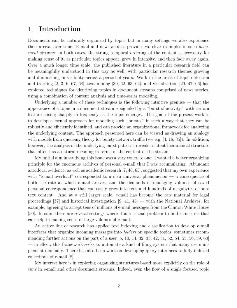
An infinite-state model. Consider a sequence of n+1 messages that arrive over a period

of time of length T . If the messages were spaced completely evenly over this time interval,

then they would arrive with gaps of size g = T/n. Bursts of greater and greater intensity

would be associated with gaps smaller and smaller than g. This suggests focusing on an

infinite-state automaton whose states correspond to gap sizes that may be arbitrarily small,

so as to capture the full range of possible bursts. The development here will use a cost model

6

0 1 32

γ ln n per state

20 1 3

tree representation

0 1 32

bursts

b)

time

optimal state sequence

a) q q q q0 1 2 3 qi

transition cost transition cost 0 emissions at rate-1 s ig

Figure 1: An infinite-state model for bursty sequences. (a) The infinite-state automaton A∗s,γ ; in state qi,

messages are emitted at a spacing in time that is distributed according to f(x) = αie−αix, where αi = g−1si.

There is a cost to move to states of higher index, but not to states of lower index. (b) Given a sequence

of gaps between message arrivals, an optimal state sequence in A∗s,γ is computed. This gives rise to a set

of nested bursts: intervals of time in which the optimal state has at least a certain index. The inclusions

among the set of bursts can be naturally represented by a tree structure.

as in the two-state case, where the underlying goal is to find a state sequence of minimum

cost.

Thus, consider an automaton with a “base state” q0 that has an associated exponential

density function f0 with rate α0 = g−1 = n/T — consistent with completely uniform message

arrivals. For each i > 0, there is a state qi with associated exponential density fi having

rate αi = g−1si, where s > 1 is a scaling parameter. (i will be referred to as the index of

the state qi.) In other words, the infinite sequence of states q0, q1, . . . models inter-arrival

gaps that decrease geometrically from g; there is an expected rate of message arrivals that

intensifies for larger and larger values of i. Finally, for every i and j, there is a cost τ(i, j)

associated with a state transition from qi to qj. The framework allows considerable flexibility

in formulating the cost function; for the work described here, τ(·, ·) is defined so that the cost

of moving from a lower-intensity burst state to a higher-intensity one is proportional to the

number of intervening states, but there is no cost for the automaton to end a higher-intensity

7

burst and drop down to a lower-intensity one. Specifically, when j > i, moving from qi to qj

incurs a cost of (j − i)γ ln n, where γ > 0 is a parameter; and when j < i, the cost is 0. See

Figure 1(a) for a schematic picture.

This automaton, with its associated parameters s and γ, will be denoted A∗s,γ. Given

a sequence of positive gaps x = (x1, x2, . . . , xn) between message arrivals, the goal — by

analogy with the two-state model above — is to find a state sequence q = (qi1 , . . . , qin) that

minimizes the cost function

c (q | x) =

(

n−1∑

t=0

τ(it, it+1)

)

+

(

n∑

t=1

− ln fit(xt)

)

.

(Let i0 = 0 in this expression, so that A∗s,γ starts in state q0.) Since the set of possible q

is infinite, one cannot automatically assert that the minimum is even well-defined; but this

will be established in Theorem 2.1 below. As before, minimizing the first term is consistent

with having few state transitions — and transitions that span only a few distinct states —

while minimizing the second term is consistent with passing through states whose rates agree

closely with the inter-arrival gaps. Thus, the combined goal is to track the sequence of gaps

as well as possible without changing state too much.

Observe that the scaling parameter s controls the “resolution” with which the discrete

rate values of the states are able to track the real-valued gaps; the parameter γ controls the

ease with which the automaton can change states. In what follows, γ will often be set to a

default value of 1; we can use A∗s to denote A∗

s,1.

Computing a minimum-cost state sequence. Given a a sequence of positive gaps

x = (x1, x2, . . . , xn) between message arrivals, consider the algorithmic problem of finding a

state sequence q = (qi1 , . . . , qin) in A∗s,γ that minimizes the cost c (q | x); such a sequence

will be called optimal. To establish that the minimum is well-defined, and to provide a means

of computing it, it is useful to first define a natural finite restriction of the automaton: for a

natural number k, one simply deletes all states but q0, q1, . . . , qk−1 from A∗s,γ, and denotes the

resulting k-state automaton by Aks,γ. Note that the two-state automaton A2

s,γ is essentially

equivalent (by an amortization argument) to the probabilistic two-state model described

earlier.

It is not hard to show that computing an optimal state sequence in A∗s,γ is equivalent to

doing so in one of its finite restrictions.

Theorem 2.1 Let δ(x) = minni=1 xi and

k = d1 + logs T + logs δ(x)−1e.

(Note that δ(x) > 0, since all gaps are positive.) If q∗ is an optimal state sequence in Aks,γ,

then it is also an optimal state sequence in A∗s,γ.

8

Proof. Let q∗ = (q`1 , . . . , q`n) be an optimal state sequence in Ak

s,γ, and let q = (qi1 , . . . , qin)

be an arbitrary state sequence in A∗s,γ. As before, set `0 = i0 = 0, since both sequences start

in state q0; for notational purposes, it is useful to define `n+1 = in+1 = 0 as well. The goal

is to show that c (q∗ | x) ≤ c (q | x).

If q does not contain any states of index greater than k − 1, this inequality follows from

the fact that q∗ is an optimal state sequence in Aks,γ. Otherwise, consider the state sequence

q′ = (qi′1, . . . , qi′

n) where i′t = min(it, k − 1). It is straightforward to verify that

n−1∑

t=0

τ(i′t, i′t+1) ≤

n−1∑

t=0

τ(it, it+1).

Now, for a particular choice of t between 1 and n, consider the expression − ln fj(xt) =

αjxt− ln αj; what is the value of j for which it is minimized? The function h(α) = αxt− ln α

is concave upwards over the interval (0,∞), with a global minimum at α = x−1t . Thus, if j∗

is such that αj∗ ≤ x−1t ≤ αj∗+1, then the minimum of − ln fj(xt) is achieved at one of j∗ or

j∗ + 1; moreover, if j ′′ ≥ j ′ ≥ j∗ + 1, then − ln fj′′(xt) ≥ − ln fj′(x).

Since k = d1 + logs T + logs δ(x)−1e, one has

αk−1 = g−1sk−1 =n

T· sk−1 ≥

1

T· slog

sT+log

sδ(x)−1

=1

T

T

δ(x)=

1

δ(x).

Since δ(x)−1 ≥ x−1t for any t = 1, 2, . . . , n, the index k − 1 is at least as large as the j

for which − ln fj(xt) is minimized. It follows that for those t for which it 6= i′t one has

− ln fi′t(xt) ≤ − ln fit(xt), since it > i′t = k − 1.

Combining these inequalities for the state transition costs and the gap costs, one obtains

c (q′ | x) =

(

n−1∑

t=0

τ(i′t, i′t+1)

)

+

(

n∑

t=1

− ln fi′t(xt)

)

≤

(

n−1∑

t=0

τ(it, it+1)

)

+

(

n∑

t=1

− ln fit(xt)

)

= c (q | x) .

Since q′ is a state sequence in Aks,γ, and since q∗ is an optimal state sequence for this

automaton, it follows that c (q∗ | x) ≤ c (q′ | x) ≤ c (q | x).

In view of the theorem, it is enough to give an algorithm that computes an optimal state

sequence in an automaton of the form Aks,γ. This can be done by adapting the standard

forward dynamic programming algorithm used for hidden Markov models [53] to the model

and cost function defined here: One defines Cj(t) to be the minimum cost of a state sequence

for the input x1, x2, . . . , xt that must end with state qj, and then iteratively builds up the

values of Cj(t) in order of increasing t using the recurrence relation Cj(t) = − ln fj(xt) +

min`(C`(t − 1) + τ(`, j)) with initial conditions C0(0) = 0 and Cj(0) = ∞ for j > 0. In

9

all the experiments here, an optimal state sequence in A∗s,γ can be found by restricting to a

number of states k that is a very small constant, always at most 25.

Note that although the final computation of an optimal state sequence is carried out by

recourse to a finite-state model, working with the infinite model has the advantage that a

number of states k is not fixed a priori; rather, it emerges in the course of the computation,

and in this way the automaton A∗s,γ essentially “conforms” to the particular input instance.

3 Hierarchical Structure and E-mail Streams

Extracting hierarchical structure. From an algorithm to compute an optimal state

sequence, one can then define the basic representation of a set of bursts, according to a

hierarchical structure.

For a set of messages generating a sequence of positive inter-arrival gaps x = (x1, x2, . . . , xn),

suppose that an optimal state sequence q = (qi1 , qi2 , . . . , qin) in A∗s,γ has been determined.

Following the discussion of the previous section, we can formally define a burst of intensity

j to be a maximal interval over which q is in a state of index j or higher. More precisely,

it is an interval [t, t′] so that it, . . . , it′ ≥ j but it−1 and it′+1 are less than j (or undefined if

t − 1 < 0 or t′ + 1 > n).

It follows that bursts exhibit a natural nested structure: a burst of intensity j may contain

one or more sub-intervals that are bursts of intensity j + 1; these in turn may contain sub-

intervals that are bursts of intensity j +2; and so forth. This relationship can be represented

by a rooted tree Γ, as follows. There is a node corresponding to each burst; and node v is

a child of node u if node u represents a burst Bu of intensity j (for some value of j), and

node v represents a burst Bv of intensity j + 1 such that Bv ⊆ Bu. Note that the root of Γ

corresponds to the single burst of intensity 0, which is equal to the whole interval [0, n].

Thus, the tree Γ captures hierarchical structure that is implicit in the underlying stream.

Figure 1(b) shows the transformation from an optimal state sequence, to a set of nested

bursts, to a tree.

Hierarchy in an e-mail stream. Let us now return to one of the initial motivations for

this model, and consider a stream of e-mail messages. What does the hierarchical structure

of bursts look like in this setting?

I applied the algorithm to my own collection of saved e-mail, consisting of messages sent

and received between June 9, 1997 and August 23, 2001. (The cut-off dates are chosen here

so as to roughly cover four academic years.) First, here is a brief summary of this collection.

Every piece of mail I sent or received during this period of time, using my cs.cornell.edu e-

mail address, can be viewed as belonging to one of two categories: first, messages consisting

of one or more large files, such as drafts of papers mailed between co-authors (essentially,

e-mail as file transfer); and second, all other messages. The collection I am considering here

consists simply of all messages belonging to the second, much larger category; thus, to a

10

rough approximation, it is all the mail I sent and received during this period, unfiltered

by content but excluding long files. It contains 34344 messages in UNIX mailbox format,

totaling 41.7 megabytes of ascii text, excluding message headers.1

Subsets of the collection can be chosen by selecting all messages that contain a particular

string or set of strings; this can be viewed as an analogue of a “folder” of related messages,

although messages in the present case are related not because they were manually filed

together but because they are the response set to a particular query. Studying the stream

induced by such a response set raises two distinct but related questions. First, is it in fact the

case that the appearance of messages containing particular words exhibits a “spike,” in some

informal sense, in the (temporal) vicinity of significant times such as deadlines, scheduled

events, or unexpected developments? And second, do the algorithms developed here provide

a means for identifying this phenomenon?

In fact such spikes appear to be quite prevalent, and also rich enough that the algo-

rithms of the previous section can extract hierarchical structure that in many cases is quite

deep. Moreover, the algorithms are efficient enough that computing a representation for

the bursts on a query to the full e-mail collection can be done in real-time, using a simple

implementation on a standard PC.

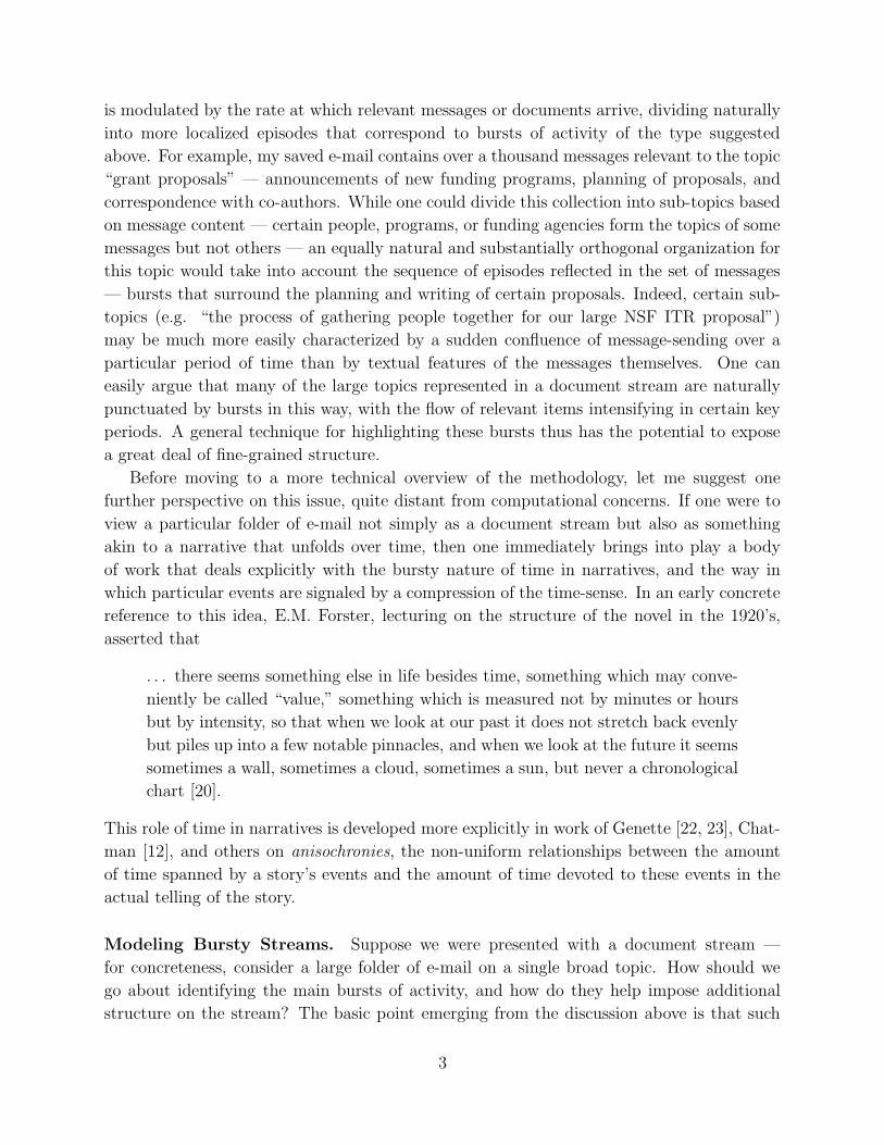
To give a qualitative sense for the kind of structure one obtains, Figures 2 and 3 show the

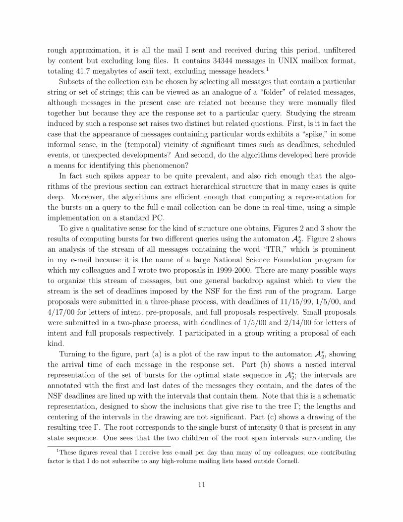
results of computing bursts for two different queries using the automaton A∗2. Figure 2 shows

an analysis of the stream of all messages containing the word “ITR,” which is prominent

in my e-mail because it is the name of a large National Science Foundation program for

which my colleagues and I wrote two proposals in 1999-2000. There are many possible ways

to organize this stream of messages, but one general backdrop against which to view the

stream is the set of deadlines imposed by the NSF for the first run of the program. Large

proposals were submitted in a three-phase process, with deadlines of 11/15/99, 1/5/00, and

4/17/00 for letters of intent, pre-proposals, and full proposals respectively. Small proposals

were submitted in a two-phase process, with deadlines of 1/5/00 and 2/14/00 for letters of

intent and full proposals respectively. I participated in a group writing a proposal of each

kind.

Turning to the figure, part (a) is a plot of the raw input to the automaton A∗2, showing

the arrival time of each message in the response set. Part (b) shows a nested interval

representation of the set of bursts for the optimal state sequence in A∗2; the intervals are

annotated with the first and last dates of the messages they contain, and the dates of the

NSF deadlines are lined up with the intervals that contain them. Note that this is a schematic

representation, designed to show the inclusions that give rise to the tree Γ; the lengths and

centering of the intervals in the drawing are not significant. Part (c) shows a drawing of the

resulting tree Γ. The root corresponds to the single burst of intensity 0 that is present in any

state sequence. One sees that the two children of the root span intervals surrounding the

1These figures reveal that I receive less e-mail per day than many of my colleagues; one contributing

factor is that I do not subscribe to any high-volume mailing lists based outside Cornell.

11

2/1410/28-

2/21/0010/28/99-

11/1610/28-

11/1611/2-

11/1511/9-

7/10/00-10/31/00

7/10-7/14

1/2-2/4

1/2-1/5

0

20

40

60

80

100

120

140

1.4e+06 1.5e+06 1.6e+06 1.7e+06 1.8e+06 1.9e+06 2e+06 2.1e+06 2.2e+06 2.3e+06 2.4e+06 2.5e+06

a)

c)

Minutes since 1/1/97

Mes

sag

e #

b)

2/14

10/28

11/161/2/00

11/16 11/15

11/2 11/9

2/4

7/10

2/21

7/10

7/14

10/31

10/28/9910/28

(large proposals)11/15: letter of intent deadline

2/14: full proposal deadline

0 1 2 3 4 5

1/2

1/5

1/5: pre-proposal deadline(large proposals)

4/17: full proposal deadline(large proposals)

7/11: unofficial notification

9/13: official announcementof awards

intensities

(small proposals)

(small proposal)

Figure 2: The stream of all e-mail messages containing the word “ITR,” analyzed using the automaton A∗2.

(a) The raw input data: the x-axis shows message arrival time; the y-axis shows message sequence number.(b) The set of bursts in the optimal state sequence for A∗

2, drawn schematically to show the inclusions that

form the tree Γ. (Lengths of intervals are standardized and hence not to scale.) Intervals are annotated withstarting and ending dates, and the dates of the NSF ITR program deadlines are lined up with the intervalsthat contain them. (c) A representation of the tree Γ, showing inclusions among the bursts.

submission deadlines and notification dates, respectively. Moreover, the sub-tree rooted at

the first of these children splits further into two sub-trees that are concentrated over a week

leading up to the deadline for letters of intent (11/15/99), and four days leading up to the

pre-proposal deadline (1/5/00). Finally, note that there is no burst of positive intensity over

the final deadline for large proposal, since we did not continue our large submission past the

pre-proposal stage.

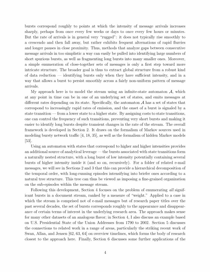
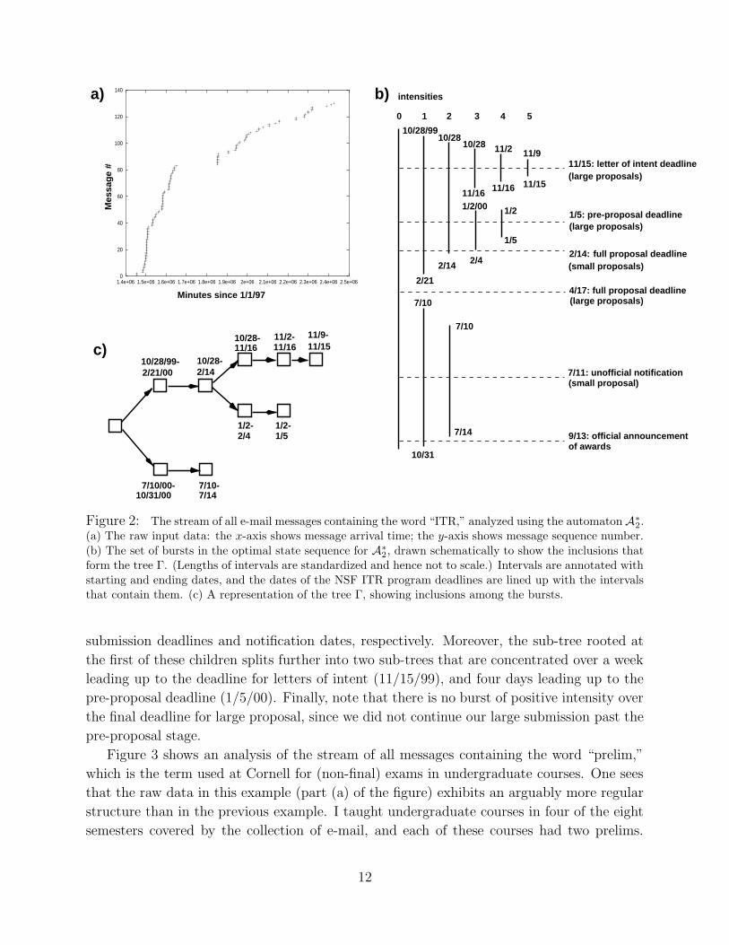
Figure 3 shows an analysis of the stream of all messages containing the word “prelim,”

which is the term used at Cornell for (non-final) exams in undergraduate courses. One sees

that the raw data in this example (part (a) of the figure) exhibits an arguably more regular

structure than in the previous example. I taught undergraduate courses in four of the eight

semesters covered by the collection of e-mail, and each of these courses had two prelims.

12

prelim 24/11/00

prelim 12/24/00

prelim 24/15/99

prelim 12/25/99

11/13/00prelim 2

1 2 3 40 5 6 7 8

prelim 110/4/00

intensities

0

50

100

150

200

250

300

350

400

200000 400000 600000 800000 1e+06 1.2e+06 1.4e+06 1.6e+06 1.8e+06 2e+06 2.2e+06 2.4e+06

Minutes since 1/1/97

Mes

sag

e #

a)

c)

b)

Figure 3: The stream of all messages containing the word “prelim,” analyzed using A∗2. Parts (a),

(b), and (c) are analogous to Figure 2, but date annotations are omitted. In part (b), the dates of prelims

(exams) are lined up with the intervals that contain them.

For the first of these courses, correspondence with students was restricted almost exclusively

to a special course e-mail account, and hence very little appears in my own saved e-mail.

The remaining three courses are captured very cleanly by the tree Γ computed from the

optimal state sequence of A∗2 (parts (b) and (c) of the figure) — each course corresponds to

a long burst, and each contains two shorter, more intense bursts for the particular prelims.

Specifically, the three children of the root are centered over the semesters in which the three

undergraduate courses were taught (Spring 1999, Spring 2000, and Fall 2000); and the sub-

trees below these children split further into two sub-trees each, concentrated either directly

over or slightly preceding the two prelims given that semester.

Overall, these structures suggest how a large folder of e-mail might naturally be divided

into a hierarchical set of sub-folders around certain key events, based only on the rate of

message arrivals. The appropriateness of Forster’s comments on the time-sense in narratives

is also fairly striking here: when organized by burst intensities, the period of time covered

in the e-mail collection very clearly “piles up into a few notable pinnacles” [20], rather than

13

proceeding uniformly.

4 Enumerating Bursts

Given a framework for identifying bursts, it becomes possible to perform a type of enumer-

ation: for every word w that appears in the collection, one computes all the bursts in the

stream of messages containing w. Combined with a method for computing a weight associ-

ated with each burst, and for then ranking by weight, this essentially provides a way to find

the terms that exhibit the most prominent rising and falling pattern over a limited period of

time. This can be applied to e-mail, and it can be done very efficiently even on the scale of

the e-mail corpus from the previous section; roughly speaking, it can be performed in a single

pass over an inverted index for the collection, and it produces a set of bursts that correspond

to natural episodes of the type suggested earlier. In the present section, however, I focus

primarily on a different setting for this technique: extracting bursts in term usage from the

titles of conference papers. Two distinct sources of data will be used here: the titles of all

papers from the database conferences SIGMOD and VLDB for the years 1975-2001; and the

titles of all papers from the theory conferences STOC and FOCS for the years 1969-2001.

The first issue that must be addressed concerns the underlying model: unlike e-mail

messages, which arrive continuously over time, conference papers appear in large batches

— essentially, twenty to sixty new papers appear together every half year. As a result,

the automaton A∗s,γ is not appropriate, since it is fundamentally based on analyzing the

distribution of inter-arrival gaps. Instead, one needs to model a related kind of phenomenon:

documents arrive in discrete batches; in each new batch of documents, some are relevant (in

the present case, their titles contain a particular word w) and some are irrelevant. The

idea is thus to find an automaton model that generates batched arrivals, with particular

fractions of relevant documents. A sequence of batched arrivals could be considered bursty

if the fraction of relevant documents alternates between reasonably long periods in which

the fraction is small and other periods in which it is large.

Suppose there are n batches of documents; the tth batch contains rt relevant documents

out of a total of dt. Let R =∑n

t=1 rt and D =∑n

t=1 dt. Now we define an automaton B∗s,γ by

close analogy with the construction of A∗s,γ. For each state qi of B∗

s,γ, for i ≥ 0, there is an

expected fraction of relevant documents pi. Set p0 = R/D, and pi = p0si. Since it does not

make sense for pi to exceed 1, the state qi will only be defined for i such that pi ≤ 1; thus,

B∗s,γ will be a finite-state automaton. One can further restrict B∗

s,γ to k states, resulting in

the automaton Bks,γ. Viewed in a generative fashion, state qi produces a mixture of relevant

and irrelevant documents according to a binomial distribution with probability pi.

The cost of a state sequence q = (qi1 , . . . , qin) in B∗s,γ is defined as follows. If the automa-

ton is in state qi when the tth batch arrives, a cost of

σ(i, rt, dt) = − ln

[(

dt

rt

)

prt

i (1 − pi)dt−rt

]

14

Word Interval of burst

data 1975 SIGMOD — 1979 SIGMOD

base 1975 SIGMOD — 1981 VLDB

application 1975 SIGMOD — 1982 SIGMOD

bases 1975 SIGMOD — 1982 VLDB

design 1975 SIGMOD — 1985 VLDB

relational 1975 SIGMOD — 1989 VLDB

model 1975 SIGMOD — 1992 VLDB

large 1975 VLDB — 1977 VLDB

schema 1975 VLDB — 1980 VLDB

theory 1977 VLDB — 1984 SIGMOD

distributed 1977 VLDB — 1985 SIGMOD

data 1980 VLDB — 1981 VLDB

statistical 1981 VLDB — 1984 VLDB

database 1982 SIGMOD — 1987 VLDB

nested 1984 VLDB — 1991 VLDB

deductive 1985 VLDB — 1994 VLDB

transaction 1987 SIGMOD — 1992 SIGMOD

objects 1987 VLDB — 1992 SIGMOD

object-oriented 1987 SIGMOD — 1994 VLDB

parallel 1989 VLDB — 1996 VLDB

object 1990 SIGMOD — 1996 VLDB

mining 1995 VLDB —

server 1996 SIGMOD — 2000 VLDB

sql 1996 VLDB — 2000 VLDB

warehouse 1996 VLDB —

similarity 1997 SIGMOD —

approximate 1997 VLDB —

web 1998 SIGMOD —

indexing 1999 SIGMOD —

xml 1999 VLDB —

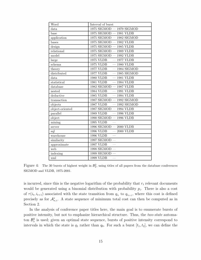
Figure 4: The 30 bursts of highest weight in B2

2, using titles of all papers from the database conferences

SIGMOD and VLDB, 1975-2001.

is incurred, since this is the negative logarithm of the probability that rt relevant documents

would be generated using a binomial distribution with probability pi. There is also a cost

of τ(it, it+1) associated with the state transition from qit to qit+1, where this cost is defined

precisely as for A∗s,γ. A state sequence of minimum total cost can then be computed as in

Section 2.

In the analysis of conference paper titles here, the main goal is to enumerate bursts of

positive intensity, but not to emphasize hierarchical structure. Thus, the two-state automa-

ton B2s is used; given an optimal state sequence, bursts of positive intensity correspond to

intervals in which the state is q1 rather than q0. For such a burst [t1, t2], we can define the

15

Word Interval of burst

grammars 1969 STOC — 1973 FOCS

automata 1969 STOC — 1974 STOC

languages 1969 STOC — 1977 STOC

machines 1969 STOC — 1978 STOC

recursive 1969 STOC — 1979 FOCS

classes 1969 STOC — 1981 FOCS

some 1969 STOC — 1980 FOCS

sequential 1969 FOCS — 1972 FOCS

equivalence 1969 FOCS — 1981 FOCS

programs 1969 FOCS — 1986 FOCS

program 1970 FOCS — 1978 STOC

on 1973 FOCS — 1976 STOC

complexity 1974 STOC — 1975 FOCS

problems 1975 FOCS — 1976 FOCS

relational 1975 FOCS — 1982 FOCS

logic 1976 FOCS — 1984 STOC

vlsi 1980 FOCS — 1986 STOC

probabilistic 1981 FOCS — 1986 FOCS

how 1982 STOC — 1988 STOC

parallel 1984 STOC — 1987 FOCS

algorithm 1984 FOCS — 1987 FOCS

graphs 1987 STOC — 1989 STOC

learning 1987 FOCS — 1997 FOCS

competitive 1990 FOCS — 1994 FOCS

randomized 1992 STOC — 1995 STOC

approximation 1993 STOC —

improved 1994 STOC — 2000 STOC

codes 1994 FOCS —

approximating 1995 FOCS —

quantum 1996 FOCS —

Figure 5: The 30 bursts of highest weight in B2

2, using titles of all papers from the theory conferences

STOC and FOCS, 1969-2001.

weight of the burst to bet2∑

t=t1

(σ(0, rt, dt) − σ(1, rt, dt)).

In other words, the weight is equal to the improvement in cost incurred by using state q1

over the interval rather than state q0. Observe that in an optimal sequence, the weight of

every burst is non-negative. Intuitively, then, bursts of larger weight correspond to more

prominent periods of elevated activity. (This notion of weight can be naturally extended to

larger numbers of states, as well as to the automaton model from Section 2.)

In Figure 4, this framework is applied to the titles of SIGMOD and VLDB papers for the

years 1975-2001. For each word w (including stop-words), an input to B22 is constructed in

16

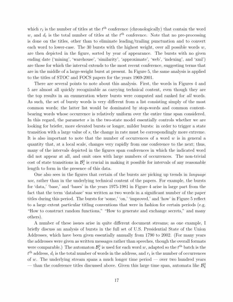
which rt is the number of titles at the tth conference (chronologically) that contain the word

w, and dt is the total number of titles at the tth conference. Note that no pre-processing

is done on the titles, other than to eliminate leading/trailing punctuation and to convert

each word to lower-case. The 30 bursts with the highest weight, over all possible words w,

are then depicted in the figure, sorted by year of appearance. The bursts with no given

ending date (‘mining’, ‘warehouse’, ‘similarity’, ‘approximate’, ‘web’, ‘indexing’, and ‘xml’)

are those for which the interval extends to the most recent conference, suggesting terms that

are in the middle of a large-weight burst at present. In Figure 5, the same analysis is applied

to the titles of STOC and FOCS papers for the years 1969-2001.

There are several points to note about this analysis. First, the words in Figures 4 and

5 are almost all quickly recognizable as carrying technical content, even though they are

the top results in an enumeration where bursts were computed and ranked for all words.

As such, the set of bursty words is very different from a list consisting simply of the most

common words; the latter list would be dominated by stop-words and common content-

bearing words whose occurrence is relatively uniform over the entire time span considered.

In this regard, the parameter s in the two-state model essentially controls whether we are

looking for briefer, more elevated bursts or longer, milder bursts: in order to trigger a state

transition with a large value of s, the change in rate must be correspondingly more extreme.

It is also important to note that the number of occurrences of a word w is in general a

quantity that, at a local scale, changes very rapidly from one conference to the next; thus,

many of the intervals depicted in the figures span conferences in which the indicated word

did not appear at all, and omit ones with large numbers of occurrences. The non-trivial

cost of state transitions in B2s is crucial in making it possible for intervals of any reasonable

length to form in the presence of this data.

One also sees in the figures that certain of the bursts are picking up trends in language

use, rather than in the underlying technical content of the papers. For example, the bursts

for ‘data,’ ‘base,’ and ‘bases’ in the years 1975-1981 in Figure 4 arise in large part from the

fact that the term ‘database’ was written as two words in a significant number of the paper

titles during this period. The bursts for ‘some,’ ‘on,’ ‘improved,’ and ‘how’ in Figure 5 reflect

to a large extent particular titling conventions that were in fashion for certain periods (e.g.

“How to construct random functions,” “How to generate and exchange secrets,” and many

others).

A number of these issues arise in quite different document streams; as one example, I

briefly discuss an analysis of bursts in the full set of U.S. Presidential State of the Union

Addresses, which have been given essentially annually from 1790 to 2002. (For many years

the addresses were given as written messages rather than speeches, though the overall formats

were comparable.) The automaton B2s is used for each word w, adapted so the tth batch is the

tth address, dt is the total number of words in the address, and rt is the number of occurrences

of w. The underlying stream spans a much longer time period — over two hundred years

— than the conference titles discussed above. Given this large time span, automata like B28

17

and B216 seem to be more effective than B2

2 at producing bursts corresponding to events on

a 5-10 year time scale; small values of s often lead to long bursts covering several decades.

The 150 bursts of highest weight in B216 (excluding those that span just a single year) are

listed at http://www.cs.cornell.edu/home/kleinber/kdd02.html.

One finds that many of the bursts seem to correspond naturally to national events and

issues, particularly up through the 1970’s. Beginning in the 1970’s and especially the 1980’s,

however, the number of bursts increases dramatically — in effect, a kind of burstiness in the

rate of burst appearances. This increase appears to reflect, in part, an increasing rhetorical

uniformity among the speeches, as numerous particular words start to appear annually at an

elevated rate. Thus the burst analysis of the addresses in the past few decades arguably has

the effect, to a large extent, of exposing specific trends in the construction of the speeches

themselves — repeated emphasis of particular key words, as well as an explosion, for example,

in the use of contractions (‘we’ve,’ ‘we’re,’ ‘I’m,’ ‘let’s’, and many others). While this

phenomenon is visible throughout the history of the address, it emerges particularly strongly

in recent years, compared with words that are more transparently associated with particular

events and issues.

5 Related Work

The Topic Detection and Tracking (TDT) study [2, 3, 67, 68] articulated the problem of

extracting significant topics and events from a stream of news articles, thereby framing

the type of document stream analysis questions considered here. Much of the emphasis in

the TDT study was on techniques for the on-line version of the problem, in which events

must be detected in real-time; but there was also a retrospective version in which the whole

stream could be analyzed. Similar issues have recently been addressed in the visualization

community [29, 47, 66], where the problem of visualizing the appearance and disappearance

of themes in a sequence of news stories has been explored.

Following on the TDT work, Swan, Allan, and Jensen [62, 63, 64] developed a method

for constructing overview timelines of a set of news stories. For each named entity and

noun phrase in the corpus, they perform a χ2 test to identify days on which the number of

occurrences yields a value above a certain threshold; contiguous sets of days meeting this

condition are then grouped into an interval that is added to the timeline. Thus, the high-level

structure of their approach is parallel to the enumerative method in Section 4. However, the

underlying methodology is quite different from the present work in two key respects. First,

Swan et al. note that the use of thresholds makes it difficult to construct long intervals of

activity for a single feature — such intervals are often broken apart by brief gaps in which

the feature does not occur frequently enough, and subsequent heuristics are needed to piece

them together. The present work, by modeling a burst as a state transition with costs, allows

for a long interval to naturally persist across such gaps; essentially, in place of thresholds, the

optimization problem inherent in finding a minimum-cost state sequence adaptively groups

18

nearby high-intensity intervals together when it is advantageous to do so. Second, the work

of Swan et al. does not attempt to infer any type of hierarchical structure in the appearance

of a feature.

Lewis and Knowles analyze the dynamics of message-sending over a very short time scale,

searching for features that can determine whether one message is a response to another [40].

This is applied to develop robust techniques for identifying threads, a popular metaphor

for organizing e-mail and newsgroup postings [16, 25]. In a very different context, Grosz

and Sidner develop structural models for discourse as a means of analyzing communication

[24]; their use of stack models in particular results in a nested organization that bears an

intriguing, though distant, relationship to the nested structure of bursts studied here.

The present work clearly overlaps with the large areas of time series analysis and sequence

mining [11, 28]; connections to related probabilistic frameworks such as Markov sources

[4, 18, 35] and hidden Markov models [53] have already been discussed above. Markov

source models are employed by Scott for the analysis of temporal data, with an application to

telephone fraud detection [58]. There has also been work incorporating a notion of hierarchy

into the framework of hidden Markov models [19, 49]; this goes beyond the type of automaton

used here to allow more complex kinds of hierarchies with potentially large state sets at

each “level.” Ehrich and Foith [17] propose a method for constructing a tree from a one-

dimensional time series, essentially by introducing a branch-point at each local minimum

and a leaf at each local maximum (see also [61]). In the context of the applications here, this

approach would yield trees of enormous complexity, due to the ruggedness of the underlying

temporal data, with many local minima and maxima.

The search for a minimum-cost state sequence in the automata of Section 2 and 4 can

also be viewed as a search for approximate level sets in a time series, and hence related

to the large body of work on piece-wise function approximation in both statistics and data

mining (see e.g. [26, 27, 30, 34, 36, 38, 43, 45]). In a discrete framework, work on mining

episodes and sequential patterns (e.g. [1, 13, 28, 44]) has developed algorithms to identify

particular configurations of discrete events clustered in time, in some cases obeying partial

precedence constraints on their order. Finally, there is an interesting general relationship

to work on traffic analysis in the areas of cryptography and security [57]; in that context,

temporal analysis of a message stream is crucial because the content of the messages has

been explicitly obscured.

6 Extensions and Conclusions

In the settings discussed above, the analysis has made use of both the temporal information

and the underlying content. The role of temporal data is clear; but the content of course

plays an integral role as well: Section 3 deals with streams consisting of the response set for a

particular query to a larger stream; and Section 4 considers streams with batched arrivals, in

which a particular subset of each batch is designated as relevant. And in fact, there is strong

19

evidence that the interplay between content and time is crucial here — that an arbitrary

set of messages with same sequence of arrival times would not exhibit an equally strong set

of bursts. Adapting a permutation test from Swan and Jensen [64], one can start with a

complete e-mail corpus having arrival times t1, t2, . . . , tN , choose a random permutation π,

and shuffle the corpus so that message π(i) arrives at time ti (instead of message i), for

i = 1, 2, . . . , N . The resulting shuffled corpus has the same set of arrival times and the

same messages, but the original correspondence between the two is broken; do equivalently

strong “spurious” bursts appear in this new sequence? In fact, they clearly do not: when the

weight of bursts for all words (with respect to A∗2) is computed using the e-mail corpus in

Section 3, the total weight associated with the true corpus is more than an order of magnitude

greater than the average total weight over 100 randomly shuffled versions (369,980 versus

25,141). Moreover, the shuffled versions exhibit almost no non-trivial hierarchical structure;

the average total number of words generating bursts of intensity at least 2 (i.e. inducing

trees Γ with two or more levels below the root) is 16.7 over the randomly shuffled versions,

compared with 3865 in the true corpus.

The overall framework developed here can be naturally applied to Web usage data —

for example, to clickstreams and search engine query logs, where bursts can correspond to

a collective focus of attention on a particular event, topic, or site. In particular, I have

applied the methods discussed here to Web clickstream data collected by Gay et al. [21].

The dataset in [21] was compiled as part of a study of student usage of wireless laptops:

The browser clicks of roughly 80 undergraduate students in two particular classes at Cornell

were collected (with consent) from wireless laptops over a period of two and a half months

in Spring 2000. Bursts with respect to A∗s,γ can be computed by an enumerative method, as

in Section 4: for every URL w, all bursts in the stream of visits to w are determined; the

full set of bursts is then ordered by weight. Each burst, associated with a URL w, now has

an additional quantity associated with it: the number of distinct users who visited w during

the interval of the burst. This allows one to distinguish between collective activity involving

much of the class and that of just a single user. As it turns out, if one focuses on bursts

that involve at least 10 distinct users, then many of those with the highest weight involve

the URLs of the on-line class reading assignments, centered on intervals shortly before and

during the weekly sessions at which they were discussed.

A final observation is that the use of a model based on state transitions leads to bursts

with sharp boundaries; they have clear beginnings and ends. In particular, this means that

for every burst, one can identify a single message on which the associated state transition

occurred. This is akin to the TDT study’s notion of (retrospective) first story detection

[2], although in the automaton model of the present work, identifying initial messages does

not constitute a separate problem since it follows directly from the definition of the state

transitions. In the context of e-mail, the contents of such an initial message can often serve

as a concentrated summary of the circumstances precipitating the burst — in other words,

there is frequently something in the message itself to frame the flurry of message-sending

20

that is about to occur. For example, one sees in Figure 2 that a very sharp state transition

related to the collection of “ITR” messages occurs at a single piece of e-mail on October

28, 1999; such a phenomenon suggests that this message may play an interesting role in the

overall stream. And for messages on which bursts for several different terms are initiated

simultaneously, this phenomenon is even more apparent; these messages often represent

natural “landmarks” at the beginning of long-running episodes.

In many domains, we are accumulating extensive and detailed records of our own commu-

nication and behavior. The work discussed here has been motivated by the strong temporal

character of this kind of data: it is punctuated by the sharp and sudden onset of particular

episodes, and can be organized around rising and falling patterns of activity. In many cases,

it can reveal more than we realize. And ultimately, the analysis of these underlying rhythms

may offer a means of structuring the information that arises from our patterns of interacting

and communicating.

Acknowledgements. I thank Lillian Lee for valuable discussions and suggestions through-

out the course of this work.

References

[1] R. Agrawal, R. Srikant, “Mining sequential patterns,” Proc. Intl. Conf. on Data Engi-

neering, 1995.

[2] J. Allan, J.G. Carbonell, G. Doddington, J. Yamron, Y. Yang, “Topic Detection and

Tracking Pilot Study: Final Report,” Proc. DARPA Broadcast News Transcription and

Understanding Workshop, Feb. 1998.

[3] J. Allan, R. Papka, V. Lavrenko, “On-line new event detection and tracking,” Proc.

SIGIR Intl. Conf. Information Retrieval, 1998.

[4] D. Anick, D. Mitra, M. Sondhi, “Stochastic theory of a data handling system with

multiple sources,” Bell Syst. Tech. Journal 61(1982).

[5] K. Becker, M. Cardoso, “Mail-by-Example: A visual query interface for managing large

volumes of electronic messages,’ Proc. 15th Brazilian Symposium on Databases, 2000.

[6] D. Beeferman, A. Berger, J. Lafferty, “Statistical Models for Text Segmentation,” Ma-

chine Learning 34(1999), pp. 177-210.

[7] H. Berghel, “E-mail: The good, the bad, and the ugly,” Communications of the ACM,

40:4(April 1997), pp. 11-15.

[8] A. Birrell, S. Perl, M. Schroeder, T. Wobber, The Pachyderm E-mail System, 1997, at

http://www.research.compaq.com/SRC/pachyderm/.

21

[9] T. Blanton, Ed., White House E-mail, New Press, 1995.

[10] G. Boone, “Concept features in Re:Agent, an intelligent e-mail agent,” Proc. 2nd Intl.

Conf. Autonomous Agents, 1998.

[11] C. Chatfield, The Analysis of Time Series: An Introduction, Chapman and Hall, 1996.

[12] S. Chatman, Story and Discourse: Narrative Structure in Fiction and Film, Cornell

Univ. Press, 1978.

[13] D. Chudova, P. Smyth, “Unsupervised identification of sequential patterns under a

Markov assumption,” KDD Workshop on Temporal Data Mining, 2001.

[14] W. Cohen. “Learning rules that classify e-mail.” Proc. AAAI Spring Symp. Machine

Learning and Information Access, 1996.

[15] T. Cover, P. Hart, “Nearest neighbor pattern classification,” IEEE Trans. Information

Theory IT-13(1967), pp. 21-27.

[16] W. Davison, L. Wall, S. Barber, trn, 1993

http://web.mit.edu/afs/sipb/project/trn/src/trn-3.6/.

[17] R. Ehrich, J. Foith, “Representation of Random Waveforms by Relational Trees,” IEEE

Trans. Computers, C25:7(1976).

[18] A. Elwalid, D. Mitra, “Effective bandwidth of general Markovian traffic sources and

admission control of high speed networks,” IEEE/ACM Trans. Networking 1(1993).

[19] S. Fine, Y. Singer, N. Tishby, “The hierarchical hidden Markov model: Analysis and

applications,” Machine Learning 32(1998).

[20] E.M. Forster, Aspects of the Novel, Harcourt, Brace, and World, Inc. 1927.

[21] G. Gay, M. Stefanone, M. Grace-Martin, H. Hembrooke, “The effect of wireless com-

puting in collaborative learning environments,” Intl. J. Human-Computer Interaction, to

appear.

[22] G. Genette, Narrative Discourse: An Essay in Method, English translation (J.E. Lewin),

Cornell Univ. Press, 1980.

[23] G. Genette, Narrative Discourse Revisited, English translation (J.E. Lewin), Cornell

Univ. Press, 1988.

[24] B. Grosz, C. Sidner, “Attention, intentions, and the structure of discourse,” Computa-

tional Linguistics 12(1986).

[25] T. Gruber, Hypermail, Enterprise Integration Technologies.

22

[26] V. Guralnik, J. Srivastava, “Event detection from time series data,” Intl. Conf. Knowl-

edge Discovery and Data Mining, 1999.

[27] J. Han, W. Gong, Y. Yin, “Mining Segment-Wise Periodic Patterns in Time-Related

Databases”, Proc. Intl. Conf. Knowledge Discovery and Data Mining, 1998.

[28] D. Hand, H. Mannila, P. Smyth, Principles of Data Mining, MIT Press, 2001.

[29] S. Havre, B. Hetzler, L. Nowell, “ThemeRiver: Visualizing Theme Changes over Time,”

Proc. IEEE Symposium on Information Visualization, 2000.

[30] D. Hawkins, “Point estimation of the parameters of piecewise regression models,” Ap-

plied Statistics 25(1976)

[31] B. Heckel, B. Hamann, “EmVis – A Visual e-Mail Analysis Tool,” Proc. Workshop on

New Paradigms in Information Visualization and Manipulation, in conjunction with Conf.

on Information and Knowledge Management, 1997.

[32] J. Helfman, C. Isbell, “Ishmail: Immediate identification of important information,”

AT&T Labs Technical Report, 1995.

[33] E. Horvitz, “Principles of Mixed-Initiative User Interfaces,” Proc. ACM Conf. Human

Factors in Computing Systems, 1999.

[34] D. Hudson, “Fitting segmented curves whose join points have to be estimated,” Journal

of the American Statistical Association 61(1966) pp. 1097–1129.

[35] F.P. Kelly, “Notes on effective bandwidths,” in Stochastic Networks: Theory and Ap-

plications, (F.P. Kelly, S. Zachary, I. Ziedins, eds.) Oxford Univ. Press, 1996.

[36] E. Keogh, P. Smyth, “A probabilistic approach to fast pattern matching in time series

databases,” Proc. Intl. Conf. Knowledge Discovery and Data Mining, 1997.

[37] J.I. Klein et al., Plaintiffs’ Memorandum in Support of Proposed Final Judgment,

United States of America v. Microsoft Corporation and State of New York, ex rel. At-

torney General Eliot Spitzer, et al., v. Microsoft Corporation, Civil Actions No. 98-1232

(TPJ) and 98-1233 (TPJ), April 2000.

[38] M. Last, Y. Klein, A. Kandel, “Knowledge Discovery in Time Series Databases,” IEEE

Transactions on Systems, Man, and Cybernetics 31B(2001).

[39] V. Lavrenko, M. Schmill, D. Lawrie, P. Ogilvie, D. Jensen, J. Allan, “Mining of Con-

current Text and Time-Series,” KDD-2000 Workshop on Text Mining, 2000.

[40] D.D. Lewis, K.A. Knowles, “Threading electronic mail: A preliminary study,” Inf. Proc.

Management 33(1997).

23

[41] S.S. Lukesh, “E-mail and potential loss to future archives and scholarship, or, The dog

that didn’t bark,” First Monday 4(9) (September 1999), at http://firstmonday.org

[42] P. Maes, “Agents that reduce work and information overload,” Communications of the

ACM 37:7(1994), pp. 30-40.

[43] H. Mannila, M. Salmenkivi, “Finding simple intensity descriptions from event sequence

data,” Proc. Intl. Conf. on Knowledge Discovery and Data Mining, 2001.

[44] H. Mannila, H. Toivonen, A.I. Verkamo, “Discovering frequent episodes in sequences,”

Proc. Intl. Conf. on Knowledge Discovery and Data Mining, 1995.

[45] R. Martin, V. Yohai, “Data mining for unusual movements in temporal data,” KDD

Wkshp. Temporal Data Mining, 2001.

[46] M.L. Markus, “Finding a Happy Medium: Explaining the Negative Effects of Electronic

Communication on Social Life at Work,” ACM Trans. Info. Sys. 12(1994), pp. 119-149.

[47] N. Miller, P. Wong, M. Brewster, H. Foote, “Topic Islands: A Wavelet-Based Text

Visualization System,” Proc. IEEE Visualization, 1998.

[48] R. Moore, C. Baru, A. Rajasekar, B. Ludaescher, R. Marciano, M. Wan, W. Schroeder,

A. Gupta, “Collection-Based Persistent Digital Archives – Part 2,” D-Lib Magazine,

6(2000).

[49] K. Murphy, M. Paskin, “Linear time inference in hierarchical HMMs,” Advances in

Neural Information Processing Systems (NIPS) 14, 2001.

[50] F. Olsen, “Facing Flood of E-Mail, Archives Seeks Help From Supercomputer Re-

searchers,” Chronicle of Higher Education, August 24, 1999.

[51] T. Payne, P. Edwards, “Interface agents that learn: An investigation of learning issues

in a mail agent interface,” Applied Artificial Intelligence 11(1997), pp. 1–32.

[52] S. Pollock, “A rule-based message filtering system,” ACM Trans. Office Automation

Systems 6(3):232–254, 1988.

[53] L. Rabiner, “A tutorial on hidden Markov models and selected applications in speech

recognition,” Proc. IEEE 77(1989).

[54] M. Redmond, B. Adelson, “AlterEgo e-mail filtering agent,” Proc. AAAI Workshop on

Case-Based Reasoning, 1998.

[55] J. Rennie, “ifile: An application of machine learning to e-mail filtering,” Proc. KDD

Workshop on Text Mining, 2000.

24

[56] M. Sahami, S. Dumais, D. Heckerman, E. Horvitz. “A Bayesian approach to filtering

junk email,” Proc. AAAI Workshop on Learning for Text Categorization, 1998.

[57] B. Schneier, Applied Cryptography Wiley, 1996.

[58] S.L. Scott, Bayesian Methods and Extensions for the Two State Markov Modulated

Poisson Process, Ph.D. Thesis, Harvard University, Dept. of Statistics, 1998.

[59] R. Segal, J. Kephart. “MailCat: An intelligent assistant for organizing e-mail,” Proc.

Intl. Conf. Autonomous Agents, 1999.

[60] R. Segal, J. Kephart. “Incremental Learning in SwiftFile,” Proc. Intl. Conf. on Machine

Learning, 2000.

[61] S. Shaw, R. DeFigueiredo, “Structural Processing of Waveforms as Trees,” IEEE Trans-

actions on Acoustics, Speech, and Signal Processing 38:2(1990)

[62] R. Swan, J. Allan, “Extracting significant time-varying features from text,” Proc. 8th

Intl. Conf. on Information Knowledge Management, 1999.

[63] R. Swan, J. Allan, “Automatic generation of overview timelines,” Proc. SIGIR Intl.

Conf. Information Retrieval, 2000.

[64] R. Swan, D. Jensen, “TimeMines: Constructing Timelines with Statistical Models of

Word Usage,” KDD-2000 Workshop on Text Mining, 2000.

[65] S. Whittaker, C. Sidner, “E-mail overload: Exploring personal information management

of e-mail,” Proc. ACM SIGCHI Conf. on Human Factors in Computing Systems, 1996.

[66] P. Wong, W. Cowley, H. Foote, E. Jurrus, J. Thomas, “Visualizing sequential patterns

for text mining,” Proc. IEEE Information Visualization, 2000

[67] Y. Yang, T. Ault, T. Pierce, C.W. Lattimer, “Improving text categorization methods

for event tracking,” Proc. SIGIR Intl. Conf. Information Retrieval, 2000.

[68] Y. Yang, T. Pierce, J.G. Carbonell, “A Study on Retrospective and On-line Event

Detection,” Proc. SIGIR Intl. Conf. Information Retrieval, 1998.

25