Burkholder’sSharp p estimates for martingale transforms · 3 Thisthesisisaboutsomesharpinequalitiesformartingaletransforms. The martingale transform acts on a martingale X n by

Alma Mater Studiorum · Università diBologna

FACOLTÀ DI SCIENZE MATEMATICHE, FISICHE E NATURALICorso di Laurea in Matematica

Burkholder’s Sharp Lp estimatesfor martingale transforms

Tesi di Laurea in Analisi Armonica

Relatore:Chiar.mo Prof.NICOLA ARCOZZI

Presentata da:ANGELICA LONGETTI

V SessioneAnno Accademico 2015/2016

2

AbstractL’argomento della tesi è una disuguaglianza Lp per trasformate di martingala.La trasformata di una martingalaXn si ottiene moltiplicando le sue differenzeper una sequenza prevedibile Hn, ottenendo così la sequenza delle differenzedella martingala trasformata (H ·X)n.E’ interessante che siano stati identificate le stime esatei in Lp per questetrasformate.

Nella presente tesi si discuterà sulla tecnica di dimostrazione, dovuta alprobabilista BurkholderQuesta si sviluppa due parti: (i) la prova della disuguaglianza tramite una"funzione di Bellman" a due variabili con determinate proprietà e (ii) la provadell’esistenza di tale funzione, che viene costruita esplicitamente.Ciò che è sorprendente è che Burkholder sia stato in grado di individuarla.

La ricerca si è successivamente ampliata ad altre disuguaglianze, con ap-plicazioni a vari problemi di analisi stocastica, generalizzando i risultati e leidee di Burkholder in differenti contesti. Si tratta di un campo di ricercacorrente in continuo sviluppo.

3

This thesis is about some sharp inequalities for martingale transforms. Themartingale transform acts on a martingale Xn by multiplying its differencesequence times a fixed bounded, predictable process Hn, obtaing the differ-ence sequence of the transformed martingale (H ·X)n.It came as a surprise that sharp Lp bounds of such transforms could be foundand proved.

In this thesis shall explain Burkholder’s technique of proof.It rests on twosteps: (i) the inequality holds if a suitable, two-variables "Bellman function"with certain properties is known and (ii) the existence of such Bellman func-tion is proved.What is surprising is the fact that Burkholder was able to find an explicitexpression for the Bellman function for the problem Lp estimates we consider.

Much research has been done later, extending Burkholder’s methods andideas to various inequalities, applying it to various problems in stochasticanalysis, extending it to different contexts.

4

I wuold like to express my thanks and gratitudeto my supervisor and to my family.

Contents

1 Martingales and Prerequisites 91.1 Conditional Expectation and Probablity . . . . . . . . . . . . 9

1.1.1 Properties . . . . . . . . . . . . . . . . . . . . . . . . . 101.1.2 Regular Conditional Probabilities . . . . . . . . . . . . 12

1.2 Martingales . . . . . . . . . . . . . . . . . . . . . . . . . . . . 121.2.1 Martingales, supermartingales, submartingale . . . . . 121.2.2 Doob’s decomposition Theorem . . . . . . . . . . . . . 131.2.3 Predictable sequences and the impossibility of beating

the system . . . . . . . . . . . . . . . . . . . . . . . . . 141.2.4 Stopping Time . . . . . . . . . . . . . . . . . . . . . . 161.2.5 Convergence . . . . . . . . . . . . . . . . . . . . . . . . 17

2 Martingales in Optimisation Problem 192.1 Optional Stopping Theorem . . . . . . . . . . . . . . . . . . . 19

2.1.1 The Secretary Problem . . . . . . . . . . . . . . . . . . 222.2 Burkholder’s Sharp Lp Estimate for Martingale Tranfsorm . . 23

Bibliography 29

5

6 CONTENTS

Introduction

In this thesis I’m going to introduce some selected concepts about Martin-gales, aiming to prove very important theorems about optimality, in partic-ular the Burkholder’s Theorem.

After preliminary notions then I’ll introduce the Doob’s optional stoppingtheorem, first for submartingales uniformely integrable and then for martin-gales, exhibiting the conditions under which the theorem holds. To followthe famous application: the Secretary Problem.

The main topic are the Burkholder’s Lp sharp inqualities for martingaletransforms [4][5] for 1 < p <∞.The martingale transform acts on a martingale Xn by multiplying its dif-ference sequence times a fixed bounded, predictable process Hn, obtaing thedifference sequence of the transformed martingale (H ·X)n.The Burkholder results and ideas about that are nowdays important: the"method of Bellman’s functions" [6], which is a direct generalization of Burkholder’smethod, is a current area of intensive and important research.Burkholder’s proof rests on two steps:I. The inequality is proved if a two-variables "Bellman’s function" z = U(x, y)having certain properties exist.II. The existence of such function is proved [4], or, even better, the functionis exhibited [5][2]. Once the function U is exhibited, verifying its relevantproperties is an long, but standard exercise in multivariable calculus.What is surprising is the fact that Burkholder was able to find it.A few remarks about the proof are in order.First, I have considered the case of dyadic martingales only, because I thoughtsome passages were more transparent in this case and because the moderntheory of Bellman functions is set in the dyadic setting (the proof extendswithout changes to the general case of discrete martingales).Second, I give the proof for p ≥ 2 only beacuse I thought it was enough toconsider one range of the exponent to get acquainted with the techniques(the proof for 1 < p ≤ 2 is similar in spirit, but is is does not simply followsfrom "passing to the conjugate exponent").

7

8 CONTENTS

Third, I did not put in the thesis the sequence of examples showing that theconstant is the best one. Because of the short time writing I preferred toconcentrate on the presentation of the main result.

Chapter 1

Martingales and Prerequisites

Before beginning our discussion on specific properties of Martingales, weneed to remember some important prerequisites such as the conditional ex-pectiation, i.e. given information, the way in which the probability of eventschanges.

Notation: We’ll use Xn instead of Xnn≥0 such as in [1].

1.1 Conditional Expectation and ProbabilityDefinition 1.1 (Conditional Expectation). Given are a probability space(Ω,F0, P ), a σ − field F ⊂ F0, and a random variable X ∈ F0 withE | X |<∞, we define the conditional expectation ofX given F , E (X | F),tobe any random variable Y such that:

(i) Y ∈ F , i.e., Y is F -measurable,(ii) for all A ∈ F ,

∫AX dP=

∫A Y dP .

Any Y satisfying (i) and (ii) is said to be a version of E (X | F). The firstthing to be settled is that the conditional expectation exists and is unique.

Proof. , if Y’ also satisfies (i) and (ii) then∫A Y dP=

∫A Y

′ dP for all A ∈ F .

Taking A = Y − Y ′ ≥ ε > 0, we see

0=∫AX −X dP=

∫A Y − Y ′ dP ≥ ε.

so P (A) = 0. Since this holds for all ε we have Y ≤ Y ′ a.s., and interchang-ing the roles of Y and Y ′, we have Y=Y ′ a.s.

9

10 CHAPTER 1. MARTINGALES AND PREREQUISITES

(Technically, all equalities such as Y=E (X | F) should be written Y=E (X | F)a.s.).

Lemma 1.1.1.If Y satisfies (i) and (ii), then it is integrable.

Proof. Letting A=Y > 0 ∈ F , using (ii) twice, and then adding

∫A Y dP=

∫AX dP ≤

∫A | X | dP ,∫

Ac −Y dP=∫Ac −X dP ≤

∫Ac | X | dP .

So we have E | Y |≤ E | X |.

1.1.1 PropertiesTheorem 1.1.2.(a) Linearity of Conditional Expectation:

E(aX + Y | F)=aE(X | F) + E(Y | F),

(b) If X ≤ Y then

E(X | F) ≤ E(Y | F),

(c) If Xn ≥ 0 and Xn ↑ X with E(X) <∞ then

E(Xn | F) ↑ E(X | F).

Observation 1.By appying the last result to Y1 − Yn we see that if Yn ↓ Y and we haveE | Y1 |,E | Y |<∞ then E(Yn | F) ↓ E(Y | F).

Proof. To prove (a), we need to check that the right-hand side is a version ogthe left. It clearly is F -measurable. To check (ii), we observe that if A ∈ Fthen by linearity of the integral and the defining properties of E(X | F) andE(Y | F),∫

A aE(X | F) + E(Y | F) , dP=a∫AE(X | F) dP+

∫AE(Y | F) dP=

=a∫AX dP+

∫A Y dP =

∫A aX + Y dP

1.1. CONDITIONAL EXPECTATION AND PROBABLITY 11

which proves (a).

Using the definition∫AE(X | F) dP=

∫AX dP ≤

∫A Y dP=

∫AE(Y | F) dP .

Letting A = E(X | F)− E(Y | F) ≥ ε > 0, we see that the indicated sethas probability 0 for all ε > 0, and we have proved (b).

Let Yn = X −Xn. It suffices to show that E(Yn | F) ↓ 0.Since Yn ↓, (b) implies Zn ≡ E(Yn | F) ↓ a limit Z∞.If A ∈ F then∫

A Zn dP=∫A Yn dP .

Letting n −→ ∞, noting Yn ↓ 0, and using the dominated convergencetheorem gives that

∫A Z∞ dP=0 for all A ∈ F , so Z∞ ≡ 0.

Theorem 1.1.3.If F ⊂ G and E(X | G) ∈ F then E(X | F) = E(X | G).

Proof. By assumption E(X | G) ∈ F . To check the other part of definitionwe note that if A ∈ F ⊂ G then∫

AX dP=∫AE(X | G) dP .

Theorem 1.1.4 (Tower property).If F1 ⊂ F2 then E(E(X | F2) | F1)=E(X | F1).

Proof. Noticing that E(X | F1) ∈ F2, and if A ∈ F1 ⊂ F2 then∫AE(X | F1) dP=

∫AX dP=

∫AE(X | F2) dP .

Theorem 1.1.5.If X ∈ F and E | X |,E | XY |<∞ then

E(XY | F)=XE(Y | F).

Proof. The right-hand side ∈ F , so we have to check the tower property. Todo this, we use the usual four-step procedure. FIrst, suppose X = 1B withB ∈ F . In this case, if A ∈ F∫

A 1BE(X | F) dP=∫A∩B E(Y | F) dP=

∫A∩B Y dP=

∫A 1BY dP ,


so the tower property holds. The last result extends to simple X by linearity.If X, Y ≥ 0, let Xn be simple random variables that ↑ X, and use themonotone convergence rheorme to conclude that∫

AXE(Y | F) dP=∫AXY dP .

To prove the result in general, split X and Y into their positive and negativeparts.

1.1.2 Regular Conditional ProbabilitiesDefinition 1.2 (Regular Conditional Probabilities). Let (Ω,F , P ) bea probability space, X : (Ω,F)→ (S,S) a measurable map, and G a σ-field⊂ F . µ : ΩxS → [0, 1] is said to be a regular conditional distributionfor X given G if(i) For each A,ω → µ(ω,A) is a probability measure on (S,S).(ii) For a.e. ω,A→ µ(ω,A) is a probability measure on (S,S).When S = Ω and X is the identity map, µ is called a regular conditionalprobability.

1.2 Martingales

When we are talking about gambling, the stochastic process martingale isrepresenting the notion of a fair game, in which we have no profit or loss forevery gamble on average, regardless of the past gambles.In other words we can think about martingale Xn as the fortune at time nof a gambler who is betting on a fair game; submartingale as the outcomeon a favorable game and supermartingale on a unfavorable game.Martingales are not used just for gambling but they have applications onstochastic modelling. Let see some more formal definitions and importanttheorems about it.

1.2.1 Martingales, supermartingales, submartingaleDefinition 1.3 (Filtration). An increasing sequence of σ-fieds Fn.

Definition 1.4 (Adapted process). A sequence Xn is said to be adaptedprocess to Fn if Xn ∈ Fn for all n.

1.2. MARTINGALES 13

Definition 1.5 (Martingale). A sequence Xn is said to be martingale (withthe respect to Fn) if(i) E | Xn |<∞,(ii) Xn is adapted to Fn,(iii) E(Xn + 1 | Fn)=Xn for all n.

Example. Simple random walk. Consider the successive tosses of a faircoin and let ξn = 1 if nth tossis heads and ξn = −1 if nth toss is tails. LetXn = ξ1 +ξ2 + ...+ξn and Fn = σ(ξ1, ...ξn) for n ≥ 1, X0 = 0 and F0=∅,Ω.

We claim that Xn, n ≥ 0, is a martingale with the respect to Fn. To provethis, we observe that Xn ∈ Fn,E | Xn |<∞, and ξn+1 is independent of Fn,so using the linearity of conditional expectation and Bayes’ Formula:

E(Xn+1 | Fn)=E(Xn | Fn)+E(ξn+1 | Fn)=Xn + Eξn+1=Xn

Note that, in this, example, Fn=σ(X1, ..., Xn) and Fn is the smallest filtrationthat Xn is adapted to.

Definition 1.6 (Supermartingale). A sequence Xn is said to be super-martingale (with the respect to Fn) if(i) E | Xn |<∞,(ii) Xn is adapted to Fn,(iii) E(Xn+1 | Fn) ≤ Xn for all n.

Example. If the coin tosses considered above have P (ξn = 1) ≤ 1/2then the computation just completed shows E(Xn+1 | Fn) ≤ Xn, i.e., Xn is asupermartingale. In this case, Xn corresponds to betting on an unfavorablegame.

Definition 1.7 (Submartingale). A sequence Xn is said to be submartin-gale (with the respect to Fn) if(i) E | Xn |<∞,(ii) Xn is adapted to Fn,(iii) E(Xn+1 | Fn) ≥ Xn for all n.

1.2.2 Doob’s decomposition TheoremThe Doob’s decomposition theorem says that in a probability space we canmake an almost surely decomposition from every Fn-adapted stochatic pro-cess Xn with E | Xn |<∞ to a martingale and a predictable process.It’s worth considering this result about submartingales and supermartingales.


Theorem 1.2.1 (Doob’s decomposition of submartingales).Any submartingale Xn, n ≥ 0 can be written in a unique way as Xn=Mn+An,where Mn is a martingale and An is a predictable increasing sequence withA0 = 0.

Proof. We want Xn=Mn + An, E(Mn | Fn− 1)=Mn− 1, and A − n ∈Fn− 1. So we must have:

E(Xn | Fn−1)=E(Mn | Fn−1)+E(An | Fn−1)=

=Mn− 1 + An=Xn−1 − An−1 + An.

and it follows that:(a) An − An−1=E(Xn | Fn−1)−Xn−1,(b) Mn=Xn − An.Now A0 = 0 and M0=X0 by assumption, so we have An and Mn defined forall time and we have proved uniqueness.To check that our recipe works, we observe that An − An−1 ≥ 0 since Xn

is a submartingale and induction shows An ∈ Fn− 1. To see that Mn is amartingale, we use (b), An ∈ Fn− 1 and (a):

E(Mn | Fn− 1)=E(Xn − An | Fn−1)=

=E(Xn | Fn−1)− An=Xn−1 − An−1=Mn−1.

Which completes the proof.

Observation 2.If we want to decompose a supermartingale Xn we’ll obtain a martingale Mn

and a predictable decreasing sequence An with A0 = 0, the proof is similar.

1.2.3 Predictable sequences and the impossibility ofbeating the system

Suppose that Hn : n ≥ 1 is the stake of a gambler on game (at time) n.The gambler has to base his decision on Hn on the history of the game upto time n− 1 (we are saying that Hn is Fn−1-measurable).

Definition 1.8 (Predictable Sequence). Let Fn, n ≥ 0 be a filtration.Hn is said to be a predictable process if Hn ∈ Fn−1 for all n ≥ 1.

1.2. MARTINGALES 15

In practice, supposing that the game consists of flipping a coin and that foreach dollar the gambler bets he wins one dollar when the coin comes upheads and loses his dollar when the coin comes up tails.

The winnings at time n are Hn(Xn −Xn−1) and the total winnings up tothe time n are given by (H ·X)n=

∑nm=1 Hm(Xm −Xm−1).

Example. Martingale. This is a famous gambling system defined byH1 = 1 and for n ≥ 2,

Hn = 2Hn−1 if Xn−1 −Xn−2=−1 and Hn=1 if Xn−1 −Xn−2=1.

In other words the gambler doubles his bet when he loses, so if he loses ktimes and then wins, the net winning will be −1− 2...− 2k=1. This systemseems to be a "sure thing" as long as P ((Xm −Xm−1) = 1).

We want to know if the gambler can chose Hn such that the expected totalwinnings are positive.

Definition 1.9 (Martingale Transform of Xn by Hn). The process (H ·X)n is called martingale transform of Xn by Hn.

Theorem 1.2.2 (No way to beat on unfavorable game).Let Xn, n ≥ 0, be a supermartingale. If Hn ≥ 0 is predictable and each Hn

is bounded then (H ·X)n is a supermartingale.

Proof. Using the fact thtat contitional expectation is linear, (H ·X)n ∈ Fn,Hn ∈ Fn−1, and Theorem 1.1.5, we have

E((H ·X)n+1 | Fn)=(H ·X)n+E(Hn+1(Xn+1 −Xn) | Fn)=

=(H ·X)n+Hn+1E((Xn+1 −Xn) | Fn) ≤ (H ·X)n.

Since E((Xn+1 −Xn) | Fn) ≤ 0 and Hn+1 ≥ 0.

Observation 3.The same result is obviously true for submartingales and for martingales (inthe last case, withouth the restriction Hn ≥ 0).


1.2.4 Stopping TimeNow we are interessed to introduce a new concept of time, closely relatedto the concept of a gambling system, noticing the property of martingalesE(Xn)=E(X0), n ≥ 0, which can be extended to E(XN)=E(X0), N ≤ n.We can think of stopping time as the time a gambler stop gambling,considering that the decision to stop the game at time n must be measurablewith the respect to the information the gambler has at that time.

Definition 1.10 (Stopping Time). A random variable N is said to be astopping time if N = n ∈ Fn for all n <∞.

Observation 4.If we have Hn=1N≥n, then N ≥ n=N ≤ n− 1c ∈ Fn−1, so Hn is pre-dictable, and it follows from Theorem 1.2.1 that (H ·X)n=XN∧n −X0 is asupermartingale.

Theorem 1.2.3.Let X = Xn : n ≥ 0 be a martingale and N a stopping time w.r.t. X, thenthe stopped process X=

Xn : n ≥ 0

is a martingale, where:

X:=

Xn, if N > n

XN , if N ≤ n= XN∧n.

Since X0 = X0, we conclude that E(Xn)=E(X0), n ≥ 0.

Proof. (i) Since | Xn |≤ max0≤k≤n | Xk | ≤| X0 | +...+ | Xn |, we concludethat E | Xn |≤ E(| X0 |) + ...+ E(| Xn |) <∞.(ii) by definition of X.(iii) It is sufficient to use Fn=σ X0, ...Xn since σ

X0, ...Xn

⊂ Fn by

the stopping time property that N > n is determined by X0, ..., Xn.Noticing that both Xn = Xn and ˆXn+1=Xn+1 if N > n, and Xn+1=Xn ifN ≤ n yelds

Xn+1=Xn+(Xn+1-Xn)1N≥n;

ThusE(Xn+1 | Fn)= Xn+E((Xn+1 −Xn)1N≥n | Fn)=

=Xn+1N≥nE((Xn+1 −Xn) | Fn)=

=Xn+1N≥n · 0= Xn.

1.2. MARTINGALES 17

Theorem 1.2.4.If N is a stopping time and Xn a supermartingale, then XN∧n is a super-martingale.

Theorem 1.2.5.If Xn is a submartingale and N is a stopping time with P (N ≤ k) = 1 then

EX0 ≤ EXN ≤ EXk.

Proof. The Theorem above implies that XN∧n is a supermartingale, so itfollows that

E(X0)=(EXN∧0) ≤ E(XN∧k)=E(Xn).

To prove the other inequality, let Kn=1N<n=1N ≤ n− 1. Kn is predictable,so Theorem 1.2.2 implies (K · X)n=Xn − XN∧n is a submartingale and itfollows that

E(Xk)− E(XN)=E((K ·X)n) ≥ E((K ·X)0)=0.

1.2.5 ConvergenceThis gives sufficient condition for the almost sure convergence of martingalesXn to a limiting random variable.

Theorem 1.2.6.If Xn is a submartingale w.r.t. Fn and ϕ is an increasing convex functionwith E | ϕ(Xn) |≤ ∞ for all n, then ϕ(Xn) is a submartingale w.r.t. Fn.Consequently:(i) If Xn is a submartingale then (Xn − a)+ is a submartingale.(ii) If Xn is a supermarginale then Xn ∧ a is a supermartingale.

Proof. By Jensen’s inequality and the assumpions

E(ϕ(Xn+1) | Fn) ≥ ϕ(E(Xn+1) | Fn)) ≥ ϕ(Xn).

Theorem 1.2.7 (Upcrossing inequality).If Xm,m ≥ 0, is a submartingale then

(b− a)EUn ≤ E(Xn − a)+ − E(X0 − a)+ .


Proof. Let Ym = a+ (Xm− a)+. By Theorem above, Ym is a submartingale.Clearly, it upcrosses [a, b] the same number of times that Xm does, and wehave (b− a)Un ≤ (H · Y )n), since each upcrossing resultsin a profit ≥ (b−a) and a final incomplete upcrossing (if there is one) makesa nonnegative contribution to the right-hand side. Let Km = 1−Hm.Clearly, Yn−Y0=(H ·Y )n + (K ·Y )n, and it follows from Theorem 1.2.2 thatE(K · Y )n ≥ E(K · Y )0=0 so E(H · Y )n ≤ E(Yn − Y0), proving the desiredinequality.

Theorem 1.2.8 (Martingale Convergence Theroem).If Xn is a submartingale with supE(X+

n ) <∞ then as n→∞, Xn convergesa.s. to a limit X with E | X |<∞.

Proof. Since (X − a)+ ≤ X++ | a |, the upcrossing inequality implies thatE(Un) ≤ (| a | +E(X+

n ))/(b− a).As n ↑ ∞, Un ↑ U the number of upcrossing of [a, b] by the whole sequence,so if supE(X+

n ) <∞ then E(U) <∞ a.s.Since the last conclusion holds for all rational a and b,

∪a,b∈Qlim inf Xn < a < b < limsupXn has probability 0and hance lim supXn=lim inf Xn a.s., i.e., limXn exists a.s. Faout’s lemmaguarantees E(X+) ≤ lim inf E(X+

n ) <∞, so X < infty a.s.To see X > −∞, we observe that

E(X−n )=E(X+n )− E(Xn) ≤ E(X+

n )− E(X0);(since Xn is a submartingale), so another application of Fatou’s lemma shows

E(X−) ≤ lim infn→∞E(X−n ) ≤ supnE(X+n )− E(X0) <∞.

Chapter 2

Martingales in OptimisationProblem

2.1 Optional Stopping TheoremNow we want to find the conditions under which we can prove that if Xn isa submartingale, M ≤ N are stopping times, then E(XM) ≤ E(XN). Thekey to this is the following definition:

Definition 2.1 (Uniformly Integrable). A collection of random variablesXi, i ∈ I, is said to be uniformly integrable if

limn→∞(supi∈I E(| Xi |), | Xi |) > M).

A trivial example of a uniformly integrable family is a collection of randomvariables that are dominated by an integrable random variable, i.e., | Xi |≤ Ywhere E(Y ) < 1.

Theorem 2.1.1.If Xn is a uniformly integrable submartingale then for any stopping timeN ,XN∧n is uniformly integrable.

Proof. X+n is a submartingale, so Theorem 1.2.5 implies E(X+

N∧n) ≤ E(X+n ).

Since X+n is uniformely integrable, it follows from the definition that

supnE(X+N∧n) ≤ supnE(X+

n ) <∞.Using the Martingale Convergence Theorem now givesX+

N∧n → Xn a.s. (hereX∞=limnXn) and E | XN |<∞. With this established, the rest is easy. Wewrite

E(| XN∧n |;| XN∧n |> K)=E(| XN |;| XN |> K,N ≤ n)+E(| XN |;| XN |> K,N > n)

19

20 CHAPTER 2. MARTINGALES IN OPTIMISATION PROBLEM

Since E | XN |≤ ∞ and Xn is uniformly integrable, if K is large then eachterm is ε/2.

From the last computation in the proof above, we get:

Theorem 2.1.2.If E|XN | <∞ and Xn1(N>n) is uniformly integrable, then XN∧n is uniformlyintegrable.

From the Theorem 2.1.1 we also immediately get:

Theorem 2.1.3.If Xn is a uniformly integrable submartingale then for any stopping timeN ≤ ∞, we have E(X0) ≤ E(XN) ≤ E(X∞), where X∞= limXn.

Proof. Theorem 1.2.5 implies E(X0) ≤ E(XN∧n) ≤ E(Xn).Letting n→∞ and observing that Theorem 2.1.1 implies XN∧n → XN andXn → X∞ in L1 gives the desired result.

Theorem 2.1.4 (Optional Stopping Theorem).If L ≤M are stopping times and YM∧n is uniformly integrable submartingale,then E(YL) ≤ E(YM) and

YL ≤ E(YM | FL).

Proof. Use the inequality E(Xn) ≤ E(X∞) in Theorem 2.1.3 with Xn=YM∧n

and N = L. To prove the second result, let A ∈ FL and N =

L, on A

M, on Ac

is stopping time.Using the first result now shows E(YN) ≤ E(YM). Since N = M on Ac, itfollows from the last inequality and the definition of conditional expectationthat

E(YL;A) ≤ E(YM ;A)=E(E(YM | FL);A).

Taking Aε=YL − E(YM | FL) > ε, we conclude P (Aε) = 0 for all ε > 0and the desired result follows.

It is worth considering the stopping theorem on martingales, explicatingthe conditions that make sure that we have E(Xn)=E(X0):

2.1. OPTIONAL STOPPING THEOREM 21

Theorem 2.1.5 (Doob’s optional stopping Theorem).Let T be a stopping time and Xn a martingale. Then XT is integrable andE(XT )=E(X0)if one of the following conditions holds:(i) T is bounded,(ii) T is almost surely finite and X is bounded,(iii) E(T ) <∞ and there is K > 0 such that, | Xn −Xn−1 |≤ K for all n.

Proof. We assume thatXn is a supermaringale. ThenXT∧n is a supermartin-gale by Theorem 1.2.4 and in particular, it is integrable,and E(XT∧n)−X0) ≤ 0.For (i) E(XT ) ≤ E(X0) follows by chosing n=N .For (ii) E(XT ) ≤ E(X0) letting n→∞ and use dominated convergence.For (iii) we observe that | XT∧n −X0 |=|

∑T∧nk=1 (Xk −Xk−1) |≤ KT and we

can use dominated convergence to have E(XT ) ≤ E(X0).Applying the previuos considerations to supermartingales −Xn we have thestatement.

Example. The first run of three sixes. We have a fair die throw-ing independently at each time step.A gambler wins a fixed amount of money as soon as the first rum of threeconsecutive sixes appear. We want to know which is the mean number ofthrows until the gambler wins for the first time.Let X1,X2,... be the sequence of random variables representing the outcomesof the throws.We have P (Xi = k)=1/6 for every k ∈ 1, ..., 6. Let F(n)=σ(X1, ..., Xn)and T be the first time three consecutive sixes appear.T is a stopping time and we are looking for E(T ).Before each time n a gambler bets 1ethat the nth throw will show six.If he loses, he leaves, if he wins he receives 6e, all of which he bets on theevent that (n + 1)st throw will be six again and so on if he loses he leavesand if he wins he will bet in the third throw and so forth.T is a stopping time satisfying condition (iii) of Doob’s optional stoppingtheorem, so we have E(T )=6 + 62 + 63=258 which is the expected moneyspent by the gamblers.At time T the last gambler won 6e,the one before 36eand the one before216e.All other gamblers have lost their post.

More formally, let be Sn=(1 + 6 + ...+ 6k) the total stakes of all gamblers attime n if there is a run of k sixes, and let Mn=Sn − n, in particular M0=1.


Then Mn is a martingale, indeedE(Mn+1Fn)=(5/6)(1− (n+ 1)) + (1/6)(6Sn + 1− (n+ 1))=Sn − n=Mn.Need to argue that E(T ) <∞:Observing T = k we need to have at least one number which is not six inevery tuple (X3m+1, X3m+2), X3m+3 for 3m+ 3 < k henceP (T = k) ≤ (1 − 1/63)(k−3)/3=(215/216)(k−3)/3 so E(T )=∑∞k=1 kP (T = k)converges.We consider the stopped martingale MT , then considering that E(T ) < ∞as we have seen and | MT

n −MTn−1 |≤ 260, by part (iii) of Doob’s Optional

Stopping Theorem, we have 1=E(M0)=E(MT )=1 + 6 + 62 + 63 − E(T ).

2.1.1 The Secretary ProblemWe consider a known number of items presented one by one in random order,i.e. such that all n! possible orders being equally likely.We can rank at any time the items that have so far been presented in orderof usefulness. As each item is presented we must either accept it, in whichcase the process stops, or reject it, when the next item in the sequence ispresented and we have to do the same choice as before.Our aim is to maximize the probability that the item we choose is the bestof the n items available.Since we cannot never to go back and choose a previously-presented itemwhich, in retrospect, turns out to be best, we clearly need to balance thedanger of stopping too soon and accepting an item when an even better onemight be still to come, and the danger of going on too long and finding thatthe best item was alreasy rejected.

Example. There are N candidates for a job interview. Let Xi be the ithcandidate. The boss interviews each in turn and he must decide wheter toaccept or reject the candidate, with not recall of an eventual rejected candi-date.

Theorem 2.1.6.Let Xi, i ∈ 1, ..., N be random variable uniformly distribuited on [0, 1], thestopping time T ∗=inf n > 0 : Xn > αn maximises E(XT ), for αN=0 andαn−1=1/2 + α2

n/2 for 1 ≤ n ≤ N .

Proof. We want to show that for any 0 ≤ α ≤ 1, we have E(Xn ∨ α)=1/2 +α2/2. It sufficies to notice thatE(Xn ∨ α)=

∫ 10 x ∨ α dx=

∫ α0 α dx+

∫ 1α x, dx= α2 + 1/2− α2/2= 1/2 + α2/2

Now, for any stopping time T , the process Y defined by

2.2. BURKHOLDER’S SHARP LP ESTIMATE FOR MARTINGALE TRANFSORM23

Y0=α0, and Yn=(XT∧n) ∨ αn for n ≤ 1

Is a submartingale, indeed, on the event T ≤ n− 1, we have

E(Yn | Fn−1)=E(XT∧n ∨ αn | Fn−1)=XT ∨ αn ≤ XT ∨ αn−1=Yn−1.

Using that αn is decreasing. On the event T ≤ n− 1, we have

E(Yn | Fn−1)=E(XT∧n ∨ αn)= α2n/2 + 1/2

which shows the supermartingale property.Let’ see that for T = T ∗ the process Y is a martingale. Indeed, on theT ∗ ≤ n− 1, we have, from above,

E(Yn | Fn−1)=XT ∗ ∨ αn=XT ∗ as XT ∗ > αT ∗ ≥ αn−1 ≥ αn.

Noticing that Y n− 1=XT ∗ ∨ αn−1=XT ∗ , on the event T ∗ ≥ n we have, asbefore,

E(Yn | Fn−1)=E(XT∧n ∨ αn)= α2n/2 + 1/2=Yn−1.

In the end we show that for any stopping time T , we have E(XT ) ≤ E(XT ∗).For this we use Doob’s optimal stopping theorem (noticing that all stoppingtimes are bounded), to see that, for arbitrary stopping times

E(XT ) ≤ E(XT ∨ αT )=E(YT ) ≤ E(Y0)=α0

and, for the special choice T ∗,

E(XT ∗)=E(XT ∗ ∨ αT ∗)=E(YT ∗) ≤ E(Y0)=α0

and this completes the proof.

2.2 Burkholder’s Sharp Lp Estimate for Mar-tingale Tranfsorm

Before beginning our considerations about the Sharp inequality, we need tointroduce the space, the σ-algebra and the probability that we are going touse.Our space is Ω = (0, 1], on which we can define subintervals such ( (j−1)

2n , j2n ]

with 1 ≤ j ≤ 2n, the probability is P (E) =| E | i.e. the Lebesgue-measure,so P ((( (j−1)

2n , j2n ]])=1/2n.

Let Fn=σ(( (j−1)2n , j

2n ]), 1 ≤ j ≤ 2n, the ⋃nFn=F which is Borel-σ-algebra.


Theorem 2.2.1.Let Xn be a martingale in (Ω,Fn, P ) with the property thatsupnE | Xn |p< +∞, 1 < p < +∞, then Xn is uniformly integrable (i.e.there exist limn→∞Xn = X a.s. with X ∈ F=⋃nFn and Xn=E(X | Fn).

Theorem 2.2.2 (Burkholder’s Sharp Inequality).Let Xn be a martingale with the property thatsupnE | Xn |p< +∞, 1 < p < +∞ and let Hn be a predictable sequence suchthat | Hn |≤ 1 a.s.Let dn = Xn −Xn−1, n ≥ 1, and define the martingale transformYn=(H ·X)n=

∑nm=1 Hm(Xm −Xm−1).

Then:Yn is martingale in (Ω,Fn, P ), and

E | Yn |p≤ c(p)pE | Xn |p,

with c(p)=p∗ − 1=

p− 1, if p ≥ 2p′ − 1, if 1 < p < 2, p′ such that 1/p+ 1/p′ = 1

p∗ = max p, p/p− 1.

Moreover by the Theorem above we have thatthere exist Y=limn→∞ Yn = Y a.s. and then E | Y |p|≤ c(p)pE | X |p andthe constant c(p) is the best possible.

Proof. X : Ω = (0, 1]→ R is Borel-measurable, so if Xn=E(X | Fn) thenE(X | Fn)p=

∫ 10 | X(t) |p dt <∞.

E(X | Fn) is a random variable which is constant in I=((j − 1)/2n, j/2n]:

E(X | Fn)(t) =

(1/ | I |)∫I | X(t) | dt = (1/P (I))E(X1I), if t ∈ I

0, if t /∈ I

We prove that E | Y |p≤ c(p)pE | X |p by considering the functionV : R2 → R such that V (x, y) =| y |p −c(p)p | x |p, the goal is to show thatE(V (Xn, Yn)) ≤ 0.

To do that let introduce a the function U : R2 → R such that:(a) U(x, y) ≥| y |p −c(p)p | X |p,(b) U(x, 0) ≤ 0 for all x ∈ R,(c) Taking a function R → R such that t 7→ U(x + th, y + tk) then thisfunction is concave for all x, y, h, t such that | k |≤| h |.

Let U(x, y)=αp(| y |p −(p∗ − 1)) | x |)(| x |)(| x | + | y |)p−1,


with α=p(1− 1/p∗)p−1.

First, we show that (a),(b),(c) imply E | Yn |p≤ c(p)pE | Xn |p:

By (a) we have E(| Xn |p −(c(p) | Yn |p)) ≤ E(U(Xn, Yn)) then to proveE(Xn, Yn) ≤ 0 it suffices to prove that EU(Xn, Yn) ≤ 0.Let I ∈ Fn−1 and I+, I− ∈ Fn its left,right values.

E(U(Xn, Yn) | Fn−1)(I)=E(U(Xn−1 + dn, Yn−1 + dnHn) | Fn−1)(I)=

(Considering h = dn and k = dnHn we have | k |≤| h |)

by definition

=(1/2)U(Xn−1(I) + dn(I+), Yn−1(I) + dn(I+)Hn(I))++(1/2)U(Xn−1(I) + dn(I−), Yn−1(I) + dn(I−)Hn(I)). (**)

By (c) and definition of concavity we have (φ(a) + φ(b))/2 ≤ φ((a+ b)/2).Let φ(t)=U(Xn−1(I) + t, Yn−1(I)Hn(I)t) and, in particular, we have(φ(d(I+)) + φ(d(I−))/2 ≤ φ((d(I+) + d(I−))/2)=φ(0)i.e. we have (φ(d(I+)) + φ(d(I−)) ≤ φ(0).Then:

(**)=(1/2)U((Xn−1(I) + dn(I+), Yn−1(I) + dn(I+)Hn(I))++(Xn−1(I) + dn(I−), Yn−1(I) + dn(I−)Hn(I))) ≤

≤ U(Xn−1(I) + dn(I+)+dn(I−)2 , Yn−1(I) + dn(I+)+dn(I−)

2 Hn)==U(Xn−1(I) + Yn−1(I)).

Consequently E(U(Xn, Yn) | Fn−1)(I) ≤ U(Xn−1(I), Yn−1(I)) andcalculatingE for both members we haveE(U(Xn, Yn))(I) ≤ E(U(Xn−1, Yn−1))(I).

Repeating this recursively we’ll obtain

E(U(Xn, Yn))(I) ≤ E(U(Xn−1, Yn−1))(I) ≤≤ E(U(Xn−2, Yn−2))(I) ≤ ... ≤ E(U(X0, Y0))(I)=U(X0, 0) ≤ 0

by the property (b), concluding the first part of the proof.

Now we want to show that U(x, y) satisfies (a),(b),(c) for p ≥ 2 (the case1 < p ≤ 2 is similar, even if not identical):

For (a):Let x, y > 0 and p > 2 then V (x, y)=yp − (p− 1)pxpand U(x, y)=p(1− 1/p)p−1[y − (p− 1)x][x+ y]p−1, we need to proveV (x, y) ≤ U(x, y).


U(x, y) and V (x, y) are both homogeneous functions so we can use a changeof variables:

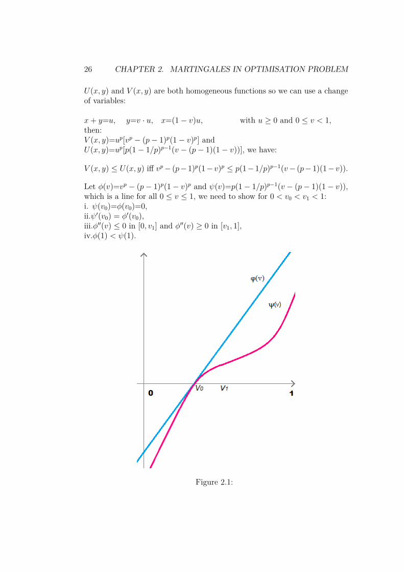
x+ y=u, y=v · u, x=(1− v)u, with u ≥ 0 and 0 ≤ v < 1,then:V (x, y)=up[vp − (p− 1)p(1− v)p] andU(x, y)=up[p(1− 1/p)p−1(v − (p− 1)(1− v))], we have:

V (x, y) ≤ U(x, y) iff vp− (p− 1)p(1− v)p ≤ p(1− 1/p)p−1(v− (p− 1)(1− v)).

Let φ(v)=vp − (p− 1)p(1− v)p and ψ(v)=p(1− 1/p)p−1(v − (p− 1)(1− v)),which is a line for all 0 ≤ v ≤ 1, we need to show for 0 < v0 < v1 < 1:i. ψ(v0)=φ(v0)=0,ii.ψ′(v0) = φ′(v0),iii.φ′′(v) ≤ 0 in [0, v1] and φ′′(v) ≥ 0 in [v1, 1],iv.φ(1) < ψ(1).

Figure 2.1:


Calculating the derivatives we obtain:φ′(v)=p[vp−1 + (p− 1)p(1− v)p−1],φ′′(v)=p(p− 1)[vp−2 − (p− 1)p(1− v)p−2].

To prove i. we notice that

φ(v0)=0 iff v01−v0

=p− 1 iff v0=p−1p=1/p′ ≥ 1/2.

Let just notice that ψ(v0) = 0.

To prove ii. we have

φ′(v0)=p[(p−1p

)p−1 + (p− 1)p(1− (p−1p

)p−1)==p(p− 1)p−1 1

pp−1 [1 + (p− 1)]=p2(1− 1/p)p−1

which is the slope of ψ, so we have ψ′(v0) = φ′(v0).

To prove iii. we notice that

φ′′(v1)=0 iff v1(1−v1)=(p− 1)

pp−2>p− 1= v0

(1−v0)

because p > p − 2 > 0 and then v1 > v0 because the function S1−S is an

increasing function on positive quadrans.

To prove iv. we have that φ(1) = 1 and ψ(1)=p(1− 1/p)p−1= (p−1)p−1

pp−2 then:

φ(1) < ψ(1) iff (p− 1)p−1 > pp−2;

let prove that (x− 1)α − xα + αxα−1 ≥ 0 for all x ≥ 1 and for all α ≥ 1,

(x− 1)α − xα=∫ 1

0ddt

(x− t)α−1 dt ≥∫ 1

0 (−α)(x− t)α−1 dt ≥≥∫ 1

0 (−α)xα−1 dt=(−α)xα−1,

by this property, for all p ≥ 2 we have(p − 1)p−1 ≥ pp−1 − (p − 1)pp−2=P p−2[p − (p − 1)]=pp−2 i.e. we proved(p− 1)p−1 > pp−2 and so iv.

To prove this properties sufficies to prove the disequality.

For (b):It is easy to see that U(x, 0)=p(1−1/p)p−1(−(p−1)x)(x)p−1 ≤ 0 when p ≥ 2.

For (c):For all x, y, h, k ∈ R, x, y > 0, p ≥ 2 as before we have:U(x, y)=p(1− 1/p)p−1[y − (p− 1)x][x+ y]p−1 and moreover

28 CHAPTER 2. MARTINGALES IN OPTIMISATION PROBLEM⟨HessU(x, y)

(hk

),(hk

)⟩=[Uxx(x, y)h] · h+ 2 [Uxy(x, y)h] · k + [Uyy(x, y)k] · k

is the directional concavity in direction (h,k).

Calculating the second derivatives we’ll obtain:Uxx=−p(p− 1)[(p− 1)x+ y](x+ y)3,Uxy=−p(p− 1)(p− 2)(x+ y)p−3x,Uyy=p(p− 1)(x+ y)p−3[y − (p− 3)x],

then:HessU(x, y)=[p(1− 1/p)p−1p(p− 1)(x+ y)p−3]

[a bc d

],

with a = −[(p− 1)x+ y], b = −(p− 2)x, c = y − (p− 3)x.We have:⟨HessU(x, y)

(hk

),(hk

)⟩=−[(p− 1)x+ y]h2 − 2(p− 2)xhk+ [y− (p− 1)x]k2=

=(y + x)(K2 + h2)− (p− 2)x(h2 + 2hk + k2)==(y + x)(K2 + h2)− (p− 2)x(h+ k)2 ≤ 0,

if | k |≤| h |.

Let G(t) = U(x+ ht, y + kt), then:G′′(t)= [Uxx(x(t), y(t))h] · h+ 2 [Uxy(x(t), y(t))h] · k + [Uyy(x(t), y(t))k] · k,

with x(t) = x+ ht, y(t) = y + kt.So G′′(t) ≤ 0 whenever | k |≤| h |.

Bibliography

[1] Durrett, Rick Probability: theory and examples. Fourth edition. Cam-bridge Series in Statistical and Probabilistic Mathematics. CambridgeUniversity Press, Cambridge, 2010. x+428 pp. ISBN: 978-0-521-76539-8

[2] Bañuelos, Rodrigo The foundational inequalities of D. L. Burkholder andsome of their ramifications. Illinois J. Math. 54 (2010), no. 3, 789-868(2012).

[3] Peter Mörters, Lecture Notes on Martingale Theory.http://people.bath.ac.uk/maspm/martingales.pdf

[4] D. L. Burkholder, Boundary value problems and sharp inequalities formartingale transforms, Ann. Probab. 12 (1984), 647-702.

[5] D. L. Burkholder, Martingales and Fourier analysis in Banach spaces,C.I.M.E. Lectures (Varenna (Como), Italy, 1985), Lecture Notes in Math-ematics, vol. 1206, Springer, Berlin, 1986, pp. 61-108.

[6] Nazarov, F. L.(1-MIS); Treil’, S. R.(1-MIS) The hunt for a Bellman func-tion: applications to estimates for singular integral operators and to otherclassical problems of harmonic analysis. (Russian. Russian summary) Al-gebra i Analiz 8 (1996), no. 5, 32–162; translation in St. Petersburg Math.J. 8 (1997), no. 5, 721-824.

29

Documents

Burkholder’sSharp p estimates for martingale transforms · 3 Thisthesisisaboutsomesharpinequalitiesformartingaletransforms. The martingale transform acts on a martingale X n by