Buoyancy effects on the integral lengthscales and mean

Buoyancy effects on the integral lengthscales and mean velocity profile inatmospheric surface layer flowsScott T. Salesky, Gabriel G. Katul, and Marcelo Chamecki Citation: Phys. Fluids 25, 105101 (2013); doi: 10.1063/1.4823747 View online: http://dx.doi.org/10.1063/1.4823747 View Table of Contents: http://pof.aip.org/resource/1/PHFLE6/v25/i10 Published by the AIP Publishing LLC. Additional information on Phys. FluidsJournal Homepage: http://pof.aip.org/ Journal Information: http://pof.aip.org/about/about_the_journal Top downloads: http://pof.aip.org/features/most_downloaded Information for Authors: http://pof.aip.org/authors

Downloaded 06 Oct 2013 to 152.3.110.48. This article is copyrighted as indicated in the abstract. Reuse of AIP content is subject to the terms at: http://pof.aip.org/about/rights_and_permissions

http://pof.aip.org/?ver=pdfcov

http://oasc12039.247realmedia.com/RealMedia/ads/click_lx.ads/www.aip.org/pt/adcenter/pdfcover_test/L-37/1781155/x01/AIP-PT/PoF_CoverPg_100213/NobelPrize_1640x440.jpg/6c527a6a7131454a5049734141754f37?x

http://pof.aip.org/search?sortby=newestdate&q=&searchzone=2&searchtype=searchin&faceted=faceted&key=AIP_ALL&possible1=Scott T. Salesky&possible1zone=author&alias=&displayid=AIP&ver=pdfcov

http://pof.aip.org/search?sortby=newestdate&q=&searchzone=2&searchtype=searchin&faceted=faceted&key=AIP_ALL&possible1=Gabriel G. Katul&possible1zone=author&alias=&displayid=AIP&ver=pdfcov

http://pof.aip.org/search?sortby=newestdate&q=&searchzone=2&searchtype=searchin&faceted=faceted&key=AIP_ALL&possible1=Marcelo Chamecki&possible1zone=author&alias=&displayid=AIP&ver=pdfcov


http://link.aip.org/link/doi/10.1063/1.4823747?ver=pdfcov

http://pof.aip.org/resource/1/PHFLE6/v25/i10?ver=pdfcov

http://www.aip.org/?ver=pdfcov


http://pof.aip.org/about/about_the_journal?ver=pdfcov

http://pof.aip.org/features/most_downloaded?ver=pdfcov

http://pof.aip.org/authors?ver=pdfcov

PHYSICS OF FLUIDS 25, 105101 (2013)

Buoyancy effects on the integral lengthscales and meanvelocity profile in atmospheric surface layer flows

Scott T. Salesky,1,a) Gabriel G. Katul,2 and Marcelo Chamecki11Department of Meteorology, The Pennsylvania State University, University Park,Pennsylvania 16802, USA2Nicholas School of the Environment, Box 90328, Duke University, Durham,North Carolina 27708, USA and Department of Civil and Environmental Engineering,Duke University, Durham, North Carolina, 27708, USA

(Received 9 January 2013; accepted 16 September 2013; published online 1 October 2013)

Within the diabatic atmospheric surface layer (ASL) under quasi-stationary and hor-izontal homogeneous conditions, the mean velocity profile deviates from its conven-tional logarithmic shape by a height-dependent universal stability correction functionφm(ζ ) that varies with the stability parameter ζ . The ζ parameter measures the relativeimportance of mechanical to buoyant production or destruction of turbulent kineticenergy (TKE) within the ASL. A link between φm(ζ ) and the spectrum of turbulencein the ASL was recently proposed by Katul et al. [“Mean velocity profile in a shearedand thermally stratified atmospheric boundary layer,” Phys. Rev. Lett. 107, 268502(2011)]. By accounting for the stability-dependence of TKE production, Katul et al.were able to recover scalings for φm with the anticipated power-law exponents forfree convective, slightly unstable, and stable conditions. To obtain coefficients for theφm(ζ ) curve in good agreement with empirical formulas, they introduced a correc-tion for the variation of the integral lengthscale of vertical velocity with ζ estimatedfrom the Kansas experiment. In the current work, the link between the coefficientsin empirical curves for φm(ζ ) and stability-dependent properties of turbulence in theASL, including the variation with ζ of the integral lengthscale and the anisotropyof momentum transporting eddies is investigated using data from the AdvectionHorizontal Array Turbulence Study. The theoretical framework presented by Katulet al. is revised to account explicitly for these effects. It is found that the coeffi-cients in the φm(ζ ) curve for unstable and near-neutral conditions can be explainedby accounting for the stability-dependence of the integral lengthscale and anisotropyof momentum-transporting eddies; however, an explanation for the observed φm(ζ )curve for stable conditions remains elusive. The effect of buoyancy on the horizontaland vertical integral lengthscales is also analyzed in detail. C© 2013 AIP PublishingLLC. [http://dx.doi.org/10.1063/1.4823747]

I. INTRODUCTION

Although atmospheric boundary layer (ABL) flows share many similarities with their flat-platecounterparts, the coexistence of mechanically and thermally generated or dissipated turbulenceuniquely distinguishes them from many wall-bounded shear flows. Diurnal variation in solar heatingand surface cooling results in the addition of buoyancy forces that alter many aspects of the flowincluding the turbulent kinetic energy (TKE) production, the topology of large eddies, and thebehavior of velocity spectra at low wavenumbers. However, in the absence of buoyancy forces, ABLflows do recover the mean velocity profile (MVP) found in the inner layer of turbulent boundarylayers. It is for this reason that buoyancy effects are treated via a so-called “stability correction” to the

a)Author to whom correspondence should be addressed. Electronic mail: [email protected].

1070-6631/2013/25(10)/105101/21/$30.00 C©2013 AIP Publishing LLC25, 105101-1


http://dx.doi.org/10.1063/1.4823747

http://dx.doi.org/10.1063/1.4823747

http://dx.doi.org/10.1063/1.4823747

mailto: [email protected]

http://crossmark.crossref.org/dialog/?doi=10.1063/1.4823747&domain=pdf&date_stamp=2013-10-01

105101-2 Salesky, Katul, and Chamecki Phys. Fluids 25, 105101 (2013)

“neutrally stratified” ABL that resembles equilibrated flat-plate boundary layers. In the atmosphericsurface layer (ASL), a region of the ABL where the immediate effects of surface roughness andCoriolis forces can be ignored, buoyancy corrections to the MVP were first considered throughdimensional analysis, carried out by Obukhov1 and Monin and Obukhov.2 As a starting point, theiranalysis assumed a stationary ASL flow over a horizontally homogeneous surface in the absenceof subsidence. Four parameters were assumed to determine the behavior of the MVP: the heightor distance from the ground surface z, the buoyancy parameter go/�0, the kinematic turbulent

shear stress at the ground τ0/ρ = u2∗ = [u′w′2 + v′w′2]1/2, and the kinematic sensible heat flux

H0/ρcp = w′θ ′, where go is the gravitational acceleration, �0 is the mean potential temperature, ρ

is the mean air density, cp is the specific heat capacity of dry air at constant pressure, H0 is the turbulentsensible heat flux (in energy flux units), u∗ is the friction velocity, u, v, w are the instantaneouscomponents of the velocity vector along the longitudinal (defined by the mean wind direction),lateral, and vertical directions, respectively, and primed quantities denote turbulent excursions fromthe mean state indicated by overbar. Upon applying dimensional analysis, an arbitrary flow statisticin the ASL can be non-dimensionalized by these variables and should universally scale with ζ = z/L,where

L = − u3∗�0

κνgow′θ ′ (1)

is the Obukhov length, and κν is the von Karman constant. This finding provided a framework toallow investigators to intercompare ASL flow statistics among different field experiments. Monin-Obukhov similarity theory (MOST) is now considered standard when reporting ASL flow statisticsand serves as a reference theory when interpreting measured deviations from these scaling arguments.In MOST, the dimensionless mean wind shear is given as

φm(ζ ) = κνz

u∗

du

dz. (2)

Under near-neutral stratification, φm(0) = 1, and (2) can be integrated to recover the conventionallogarithmic MVP. Thus, φm(ζ ) is treated as a correction to the logarithmic MVP that occur underunstable (ζ < 0) or stable (ζ > 0) stratification. MOST predicts φm (as well as other higher orderASL flow statistics) to be a function of ζ alone, but the exact form of the φm(ζ ) function mustbe determined empirically. A large number of field experiments3, 4 in the ASL have confirmed thatφm(ζ ) does indeed collapse to a universal curve when presented as a function of ζ . This apparentuniversal character of φm(ζ ) now has widespread applicability in micro-meteorology, air pollution,atmospheric chemistry, hydrology, ecology, and related disciplines, where MOST is used to estimateturbulent fluxes based on mean gradients,5–7 to parameterize surface fluxes in large-scale numericalweather prediction models,8–10 and as the basis for wall models in large eddy simulations of theABL.11, 12

Atmospheric stability (as characterized by ζ ) is known to have a significant influence onthe behavior of the temperature and velocity spectra,13 the TKE budget,14–17 and on the integralscales.13, 18 However, despite six decades of research and experimental support for MOST scaling,no theoretical link between the MVP and these fundamental, stability-dependent properties ofturbulence has been found. A framework on how to proceed with such developments was recentlyproposed19 using the “spectral link” established by Gioia et al.20 for analyzing the MVP of wall-bounded shear flows in the absence of buoyancy.

By assuming a local balance between TKE production and dissipation and accounting for thestability-dependence of TKE production in the ASL (that determines the characteristic velocity ofthe momentum-transporting eddy), Katul, Konings, and Porporato19 were able to derive a theoreticalexpression for φm(ζ ), which they showed was equivalent to the O’KEYPS equation21

[φm(ζ )]4 − γ ζ [φm(ζ )]3 = 1 (3)

with γ = 1. From their expression for φm(ζ ), Katul, Konings, and Porporato19 were able to recoverthe proper scalings for φm(ζ ) under free convective (φm ∼ ( − ζ )−1/3), slightly unstable (φm ∼ (1− ζ )−1/4), and stable (φm ∼ ζ ) conditions. However, this alone is not enough to produce a φm(ζ )



function in agreement with empirical formulas, such as the well-known Businger-Dyer22 curve:

φm(ζ ) ={

(1 − 16 ζ )−1/4, −2 ≤ ζ ≤ 0

1 + 5 ζ , 0 ≤ ζ ≤ 1. (4)

Furthermore, a value of γ greater than unity is required in the O’KEYPS equation to obtain goodagreement with experimental datasets.19 Katul, Konings, and Porporato19 hypothesized that thecoefficients of 16 and 5 in the Businger-Dyer equation are linked to stability-dependent properties ofturbulence in the ASL. By introducing a function f (ζ ) to account for the variation of the w integrallengthscale with stability (based on results from the Kansas experiment) and a correction β2 for thelocal imbalance of TKE, they were able to obtain a φm(ζ ) curve in good agreement with experimentaldata.

The goal of the current article is to investigate the linkage between the observed behavior ofφm(ζ ) and stability-dependent properties of turbulence in the ASL including the integral length-scale, the anisotropy of the momentum transporting eddies, and the TKE budget imbalance usingdata from the Advection Horizontal Array Turbulence Study (AHATS). Although Katul, Konings,and Porporato19 considered the stability-dependence of the integral scales, they assumed that themomentum-transporting eddy was isotropic in the x-z plane (i.e., having equivalent horizontal andvertical lengthscales). Here, revisions to their theoretical framework are proposed so as to unfoldthe effects of the stability dependence of the integral lengthscale and the anisotropy of momentum-transporting eddies on φm(ζ ).

The article is organized as follows. In Sec. II, prior work19 is reviewed and expanded to illustratehow φm(ζ ) is influenced by the stability-dependence of the integral lengthscale, the anisotropy of themomentum transporting eddies, and the local imbalance between TKE production and dissipation.An overview of the AHATS dataset and the data analysis procedure is then presented in Sec. III. InSec. IV, the stability dependence of the integral lengthscales is investigated using the AHATS data,and the connection between the variation with stability of the integral lengthscale and the anisotropybetween the horizontal and vertical integral scales is explored in detail. A discussion of these resultscan be found in Sec. V.

II. THEORY

In this section, the theoretical basis for the MVP in the ASL is developed based on a con-ceptual model of an ensemble momentum transporting eddy. This eddy, as sketched in Fig. 1 and

w(x + sx)

w(x − sx)

sx

sz

x

z

u(z − sz)

u(z + sz)

v(sx) = |w(x + sx) − w(x − sx)|

H0τ0

Ground

FIG. 1. Schematic diagram of an anisotropic ensemble momentum transporting eddy at height z in the ASL. The eddyis characterized by its horizontal and vertical dimensions sx and sz, and a single characteristic velocity scale v(sx ) =|w(x + sx ) − w(x − sx )|. The vertical momentum flux at height z is τt = ρ[u(z + sz) − u(z − sz)]v(sx ). Note that thecharacteristic dimensions of this ensemble eddy sx and sz will depend on atmospheric stability as characterized by ζ .



discussed below, should be viewed as a statistical entity that only exists in an ensemble mean senserather than being viewed as an alternative to conditionally sampled coherent structures (e.g., hairpinvortices23, 24) known to occur in the ASL. The subsequent discussion of the horizontal and verticaldimensions of this eddy should only be interpreted as ensemble mean quantities averaged over manyrealizations with no conditioning to exclude any subsets of events. The dimensions of this ensemblemean eddy, as characterized via the integral lengthscales determined from the autocorrelation func-tions, should not be expected to have a direct geometric correspondence to properties of spatiallylocal coherent structures.

Building upon the theoretical framework presented by previous authors,19 the mean momentumexchanged by an anisotropic eddy at height z in the ASL with horizontal and vertical dimensions ofsx and sz, respectively, is considered in Fig. 1. As evidenced by this diagram, the connection betweenthe momentum transporting eddy and the MVP is similar to Ref. 19, except that they consideredan isotropic eddy attached to the wall,25 such that sx = sz = z. Here, the eddy is allowed to retainits expected anisotropic form in the x-z plane with its horizontal and vertical dimensions allowed tovary differently with ζ . The momentum exchanged by the eddy is given as

u2∗ = κτ v(sx ) [u(sz + z) − u(sz − z)] ≈ κτ v(sx )

[du(z)

dz2sz

], (5)

where v(sx ) = |w(x + sx ) − w(x − sx )| is the characteristic eddy turnover velocity and κτ is aproportionality constant.

For the neutral ABL, sz is best represented by vertical integral length-scale of w, which isproportional to z, i.e., sz = �z

w(0) = czz, where cz is a constant of proportionality. The effects ofthermal stratification on the size of the momentum transporting eddy must be explicitly considered innon-neutral ASL flows. In this case, it is appropriate to express sz = �z

w(ζ ) = �zw(0)g(ζ ) = czzg(ζ ).

That is, sz is assumed to be equal to the actual integral length scale of w that varies with atmosphericstability, which can be formulated in terms of

g(ζ ) = �zw(ζ )

�zw(0)

, (6)

defining the ratio of the vertical integral length scale of w to its value at neutral ASL conditions.Equation (5) then becomes

2czκτ

κν

v(sx )

u∗

[du(z)

dz

κνz

u∗

]g(ζ ) = 2cz

κτ

κν

v(sx )

u∗g(ζ ) [φm] = 1. (7)

A suitable model of v(sx ), the eddy turnover velocity scale, is needed to complete the estimationof the momentum flux from the MVP. For locally homogeneous and isotropic turbulence, v(sx )can be estimated from Kolmogorov’s 4/5 law26 as earlier proposed by Gioia et al.,20 wherev(sx ) = [κεεsx ]1/3, with κε = 4/5 and ε is the TKE dissipation rate. In a neutral ASL,sx = �x

w(0) = cx z, i.e., that sx is identically the streamwise integral lengthscale of w, which isproportional to the height z. When the effects of buoyancy are considered, however, we findsx = �x

w(ζ ) = �xw(0) f (ζ ) = cx z f (ζ ), where we define

f (ζ ) = �xw(ζ )

�xw(0)

, (8)

as the ratio of the streamwise integral length scale of w to its value for neutral conditions. In thethermally stratified case, the eddy turnover velocity scale becomes

v(sx ) = [κεεcx z f (ζ )]1/3 . (9)

The assumptions of locally homogeneous and isotropic turbulence and subsequently the 4/5 lawmay not be valid at scale sx = zf (ζ ). A correction for departures from inertial subrange scaling isintroduced so that (9) becomes

v(sx ) = h(ζ ) [κεεcx z f (ζ )]1/3 , (10)



where h(ζ ) is the ratio of the “true” velocity scale calculated from the third order structure functionD111(r1) to the predicted value from the 4/5 law, i.e.,

h(ζ ) = vtrue(sx )

v4/5(sx )= [D111(r1 = z f (ζ ))]1/3

[κεεz f (ζ )]1/3 . (11)

After including these corrections, (7) becomes

2c1/3x cz

κτ

κνu∗[κεεz f (ζ )]1/3 g(ζ )h(ζ ) [φm] = 1. (12)

To obtain φm from (7), ε must now be determined. Under the assumptions of horizontallyhomogeneous, stationary, high Reynolds number flow, and in the absence of subsidence, the TKEbudget is given by27

ε = u3∗

κz[φm(ζ ) − ζ + β2(ζ )] , (13)

where β2(ζ ) is the local imbalance between TKE dissipation rate and shear + buoyant production(or destruction), and is defined by

β2(ζ ) = φε − [φm(ζ ) − ζ ] = φt + φp. (14)

By definition, the local TKE imbalance for high Reynolds number flows is also the sum of thedimensionless turbulent transport and pressure transport terms (φt and φp, respectively). Note thatthis definition of β2(ζ ) differs from that of Ref. 19, and is ζ -dependent rather than being a constantvalue. Using this ε obtained from the TKE budget, (7) becomes

2c1/3x cz

κτ

κνu∗g(ζ )h(ζ ) [φm]

[κεz f (ζ )

(u3

∗κνz

(β2(ζ ) + φm(ζ ) − ζ )

)]1/3

= 1. (15)

It can be shown that (15) reduces to

β1 [φm]4

[1 − ζ − β2(ζ )

φm(ζ )

]= 1

f (ζ )g(ζ )3h(ζ )3, (16)

where β1 = 23cx c3z κ

3τ κε

κ4ν

is a constant determined by enforcing φm(0) = 1. Equation (16) is similar toEq. (12) of Ref. 19, except that here g(ζ ) and h(ζ ) are not assumed to be unity and β2 is allowed tobe a function of ζ . In addition, as pointed out in Ref. 19, (16) can be considered as a generalizedversion of the O’KEYPS equation (3).

An alternative to considering how stability modifies the streamwise and vertical integral scales ofw separately (i.e., the functions f (ζ ) and g(ζ )) is to consider two modifications to ASL turbulence bythermal stratification. First, the integral length-scale, which characterizes the size of the momentumtransporting eddy, is modified by buoyancy; we account for this effect through the function f (ζ ).Second, buoyancy acts in such a way that the modification of the streamwise (less restricted by thepresence of the ground) and vertical (more restricted by the presence of the ground) integral length-scales of w is anisotropic with ζ . We account for this effect by defining the anisotropy correctiona(ζ ) = g(ζ )/f (ζ ), and replacing g(ζ ) with a(ζ )f (ζ ) in (16), obtaining

β1 [φm(ζ )]4

[1 − ζ − β2(ζ )

φm(ζ )

]= 1

a(ζ )3 f (ζ )4h(ζ )3. (17)

The effects of the stability corrections on φm physically represent the stability dependence of theintegral scales (f), the anisotropy of the ensemble mean momentum transporting eddy (a), departuresfrom inertial range scaling (h), and any local imbalance between TKE dissipation and productionrates (β2), and will be considered separately and jointly in Sec. IV. Note that when we discuss theanisotropy of the momentum transporting eddies, we are referring to the geometric anisotropy of thehorizontal and vertical integral lengthscales.



III. DATASET AND ANALYSIS PROCEDURE

The analysis presented in Sec. II is performed using data from the AHATS experiment conductednear Kettleman City, CA, USA from June 25 to August 16, 2008. Data from the AHATS profiletower, consisting of six Campbell Scientific CSAT-3 sonic anemometers at heights of z = 1.51,3.30, 4.24, 5.53, 7.08, and 8.05 m during the period from June 25 to July 17 were used. The fieldsite was surrounded by short grass stubble (<0.1 m in height) and was predominantly horizontallyhomogeneous and level over wind directions of |α| ≤ 45◦ included in the data analysis. The CSAT-3anemometers, which have sonic path lengths of 0.1 m, sampled the three components of the velocityvector and virtual temperature at 60 Hz; data were sub-sampled at 20 Hz during preprocessing anddivided into blocks of 27.3 min each, or 32768 = 215 data points per block (to accommodate theFFT software used to calculate spectral densities). The typical procedure of aligning the coordinatesystem with the mean wind direction so that v = 0 was followed for each block of time. Blocks ofdata were rejected if φw = σw/u∗ exhibited more than a 30% deviation from the value predicted byMOST, a common quality control criterion in micrometeorology.28 Nonstationary ratios29 for thealong-wind (RNu), cross-wind (RNv), and vector-wind (RNS) velocity components were computedand runs where RNu, RNv, or RNS ≥0.5 were excluded. The nonstationary runs were removedbecause of the large effects of nonstationarity on the lagged correlation functions, which wereneeded to estimate the integral scales. The streamwise and vertical integral length scales of w werecomputed using the measured autocorrelation function. For spatial lags in the streamwise (�x) andvertical (�z) directions, the two-point correlation function of a flow variable a(x, y, z) is defined as

ρa,a(�x , �z) = a′(x, y, z)a′(x + �x ,y,z + �z)

σa(x ,y,z)σa(x+�x ,y,z+�z), (18)

where a′ = a − a is the departure of a from its mean value, and Taylor’s frozen turbulence hypothesisis assumed to hold so that time can be interpreted as longitudinal cuts into the flow via �x = u�t .

The vertical and horizontal integral lengthscales of w were computed by applying (18) separatelyfor streamwise and vertical separations and determining the integral lengthscales through exponentialregression fitting to the measured autocorrelations, i.e.,

ρw,w(�x ,0) = exp

(−|�x |

�xw

)(19)

and

ρw,w(0,�z) = exp

(−|�z|

�zw

). (20)

Note that for the vertical autocorrelation, calculating ρw,w(�z) can be conducted using either upwardor downward vertical lags. We will denote the integral scale calculated from ρw,w(�z) using upwardlags as �z↑

w and the integral scale from downward lags as �z↓w . The difference between these two

integral scales will be discussed in Sec. IV C.The TKE dissipation rate ε was estimated from the second-order structure function D11(r1), i.e.,

D11(r1) = c2(εr1)2/3, (21)

where c2 ≈ 4.017ck, ck = 18ce/55, and ce = 1.5 is the Kolmogorov constant for the inertial range ofthe TKE spectrum E(k).30

Our estimate of ε was calculated by a linear regression to the compensated second-order structurefunction r−2/3

1 D11(r1) , i.e.,

r−2/31 D11(r1) = c2ε

2/3 = ar1 + b, (22)

using values of r1 in the range 0.2 ≤ r1 ≤ 2.0 m. The lower limit imposed on r1 ensures thatdistortions from the sonic anemometer finite path length are negligible. The upper limit on r1 isselected so as to ensure at least one decade of scales is available in the determination of ε. Theregression coefficient b was used to obtain an estimate of the dissipation rate (i.e., ε = (b/c2)3/2); thecoefficient a must be nearly zero if the data follow inertial-range scaling.



The estimate of the TKE dissipation rate ε requires the use of Taylor’s hypothesis to interprettemporal lags as spatial lags in D11(r1). However, Taylor’s hypothesis is not valid for large turbulenceintensities (defined as Iu = σu/u). Hsieh and Katul31 found that the Wyngaard and Clifford32

corrections to account for the effects of finite turbulence intensity on the structure functions werenegligible (<10%) for Iu < 0.35. We obtained Iu < 0.35 for all of the stable data, and the majorityof the unstable data from AHATS, so distortions introduced by the use of Taylor’s frozen turbulencehypothesis are not a significant source of error in the estimates of ε.

IV. RESULTS

In this section, the results from any local imbalance of the TKE budget and departures frominertial range scaling are presented along with the stability-dependence of the integral length-scales. Contributions of stability-dependent properties of turbulence (integral lengthscales and eddyanisotropy) are then propagated to effects on φm(ζ ). Specifically, we examine the local imbalanceof the TKE budget from the AHATS dataset with ζ in Sec. IV A. In Sec. IV B, we examine theeffects of departures from inertial range scaling on the eddy velocity scale. We then characterizethe stability-dependence of the integral lengthscales in Sec. IV C, considering both the horizontalintegral lengthscale of w and the vertical integral lengthscale calculated from both upward anddownward spatial lags. In Sec. IV D, we consider how the stability correction functions f (ζ ) anda(ζ ) for the integral scale and eddy anisotropy separately and jointly contribute to the variation withstability of φm. In Sec. IV E, we derive approximate solutions for φm(ζ ) in the slightly unstableand free convective limits to explicitly connect the coefficients in empirical curves for φm(ζ ) to thestability dependence of the integral scale and the eddy anisotropy.

A. Local imbalance of TKE budget

The theoretical expression for φm(ζ ) presented by Katul, Konings, and Porporato19 includesa correction for the local imbalance in the TKE budget (β2), which is zero when TKE productionbalances dissipation. Because studies of the atmospheric surface layer14–17 have revealed that thebehavior of the TKE budget is influenced by stability, we introduce a local TKE imbalance correctionas a function of ζ in the revised theory presented in Sec. II. Note that this definition of β2(ζ ), givenin (14), differs slightly from that of Ref. 19.

Calculated values of β2(ζ ) from individual runs of the AHATS data are plotted as a functionof ζ in Fig. 2(a). Here β2 is calculated from its definition in (14), and the TKE dissipation rate ε

is estimated by a linear regression (22) to the second-order structure function D11(r1). For unstableand near-neutral conditions, the TKE budget is close to a local balance (β2 ≈ 0) on average anddoes not exhibit any significant dependence on ζ . For stable conditions, β2 is slightly positiveon average, which corresponds to a local dissipation of TKE exceeding production and suggests

-3

-2

-1

0

1

2

3

-2 -1.5 -1 -0.5 0 0.5 1

β2(ζ

)

ζ

(a)

0255075

100125150175200225

0.64 0.65 0.66 0.67

PD

F(D

11

slop

e)

D11 slope

(b)

FIG. 2. (a) The local imbalance between TKE production and dissipation, β2(ζ ), as a function of the MOST stability variableζ . β2(ζ ) is calculated using ε2, the TKE dissipation rate estimated from a linear regression to the second-order structurefunction D11(r1). (b) A probability density function of the slope of D11(r1). The dashed line indicates the inertial subrangevalue of 2/3.



that flux-transport terms may be significant in sustaining turbulence in these instances. However,considerable scatter in β2 is found between individual runs for the entire range of ζ considered here,and β2 has both positive and negative values for individual blocks of data for the entire stabilityrange shown.

To determine whether estimates of ε (and therefore β2) are reasonable, the probability densityfunction (PDF) of the slope of D11(r1) from the linear regression for r1 in the range 0.2 ≤ r1 ≤ 2.0m is shown in Fig. 2(b). The mode of this PDF is close to the inertial subrange value of 2/3, anddepartures of D11 from inertial range scaling do not appear to occur frequently enough to have asignificant effect on the estimate of ε.

Although the average value of β2(ζ ) is nonzero for both unstable and stable conditions, thesedepartures from β2 = 0 appear small. More importantly, including the β2(ζ ) correction in thetheoretical expression for φm(ζ ) (17) does not have a significant influence of the behavior of φm(ζ ).For the remainder of the article, the effect of the TKE imbalance is neglected for all stabilities(β2(ζ ) = 0).

B. Departures from inertial range scaling

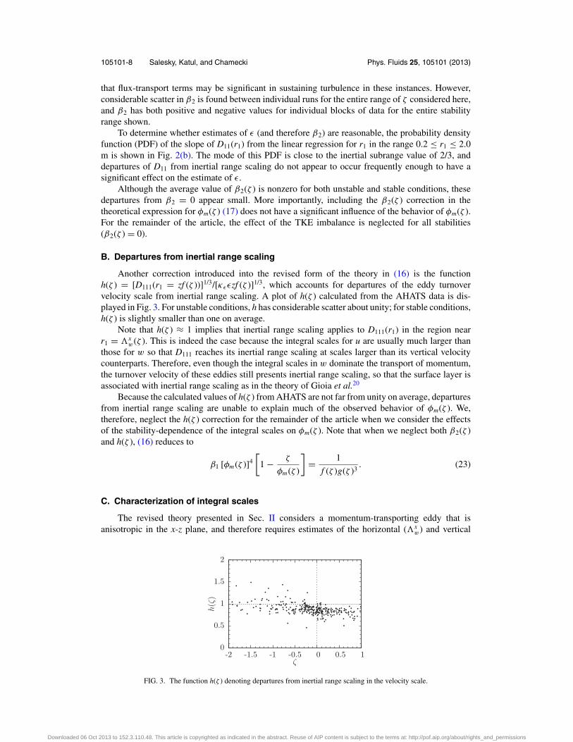
Another correction introduced into the revised form of the theory in (16) is the functionh(ζ ) = [D111(r1 = zf (ζ ))]1/3/[κεεzf (ζ )]1/3, which accounts for departures of the eddy turnovervelocity scale from inertial range scaling. A plot of h(ζ ) calculated from the AHATS data is dis-played in Fig. 3. For unstable conditions, h has considerable scatter about unity; for stable conditions,h(ζ ) is slightly smaller than one on average.

Note that h(ζ ) ≈ 1 implies that inertial range scaling applies to D111(r1) in the region nearr1 = �x

w(ζ ). This is indeed the case because the integral scales for u are usually much larger thanthose for w so that D111 reaches its inertial range scaling at scales larger than its vertical velocitycounterparts. Therefore, even though the integral scales in w dominate the transport of momentum,the turnover velocity of these eddies still presents inertial range scaling, so that the surface layer isassociated with inertial range scaling as in the theory of Gioia et al.20

Because the calculated values of h(ζ ) from AHATS are not far from unity on average, departuresfrom inertial range scaling are unable to explain much of the observed behavior of φm(ζ ). We,therefore, neglect the h(ζ ) correction for the remainder of the article when we consider the effectsof the stability-dependence of the integral scales on φm(ζ ). Note that when we neglect both β2(ζ )and h(ζ ), (16) reduces to

β1 [φm(ζ )]4

[1 − ζ

φm(ζ )

]= 1

f (ζ )g(ζ )3. (23)

C. Characterization of integral scales

The revised theory presented in Sec. II considers a momentum-transporting eddy that isanisotropic in the x-z plane, and therefore requires estimates of the horizontal (�x

w) and vertical

0

0.5

1

1.5

2

-2 -1.5 -1 -0.5 0 0.5 1

h(ζ

)

ζ

FIG. 3. The function h(ζ ) denoting departures from inertial range scaling in the velocity scale.



00.20.40.60.8

1

0 2 4 6 8 10

ρw

,w(|Δ

z|)

[–]

|Δz| [m]

z6/L6 = −0.92

(a)

00.20.40.60.8

1

0 2 4 6 8 10

ρw

,w(|Δ

z|)

[–]

|Δz| [m]

z3/L3 = −0.41

(b)

00.20.40.60.8

1

0 2 4 6 8 10

ρw

,w(|Δ

z|)

[–]

|Δz| [m]

z6/L6 = −0.02

(c)

00.20.40.60.8

1

0 2 4 6 8 10

ρw

,w(|Δ

z|)

[–]

|Δz| [m]

z3/L3 = −0.01

(d)

00.20.40.60.8

1

0 2 4 6 8 10

ρw

,w(|Δ

z|)

[–]

|Δz| [m]

z6/L6 = 0.52

(e)

00.20.40.60.8

1

0 2 4 6 8 10

ρw

,w(|Δ

z|)

[–]

|Δz| [m]

z3/L3 = 0.24

(f)

s6, fits6, data

s3↑, fits3↑, data

s3↓, fits3↓, data

FIG. 4. Calculated vertical autocorrelation of w and exponential fits used to determine the integral scale. Data from sonicanemometer 6 at 8.05 m are plotted in the top row of panels ((a), (c), and (e)), and data from sonic anemometer 3 at 4.24 mare plotted in the bottom row of panels ((b), (d), and (f)). (a) and (b) unstable, (c) and (d) near-neutral, (e) and (f) stable. Notethat the autocorrelations from sonic anemometer 3 are plotted separately for upward and downward vertical lags.

(�zw) integral lengthscales of w that characterize this eddy to evaluate the behavior of φm. Both the

horizontal and the vertical integral lengthscales were calculated by fitting an exponential curve tothe calculated autocorrelation ((19) and (20)). The behavior of the calculated vertical autocorrela-tion and the exponential fits are plotted in Fig. 4 for several individual blocks of data: an unstablecase (panels (a) and (b)), a near-neutral case (panels (c) and (d)), and a stable case (panels (e) and(f)) for measurements from the AHATS profile tower from sonic anemometer 6 at 8.05 m (toppanels) and sonic anemometer 3 at 4.24 m (bottom panels). For the autocorrelations from sonicanemometer 3 in panels (b), (d), and (f), we plot ρw,w(|�z|) for both upward and downward verticallags.

From Fig. 4, the fitted exponential curves are in reasonable agreement with the calculated auto-correlations for all stabilities and both measurement heights. This is true even for the measurementsfrom sonic anemometer 3 in the bottom panels where only 3 or 4 points were available to be used forthe exponential fits. It can be surmised that the exponential fit (20) allows reasonable estimates of thevertical integral lengthscale despite the limited number of data points. Figure 4 also demonstratesthat the correlation for a given vertical lag decreases with increasing stability, which corresponds toa decrease in the vertical integral lengthscale �z

w with increasingly stable ζ . One interesting featureof these autocorrelation curves is the difference between the autocorrelation based on upward anddownward vertical lags, as plotted in panels (b), (d), and (f) from sonic anemometer 3. When theautocorrelation is calculated taking upward lags, higher values of correlations are obtained whencompared to downward lags.

This interesting feature of the analysis can be seen more clearly in Fig. 5, where we plot boththe streamwise and vertical integral lengthscales of w normalized by z as a function of the MOSTstability parameter ζ . In Fig. 5(a), we present the streamwise integral lengthscale �x

w, and in Fig. 5(b),we present the vertical integral lengthscale �z

w. Separate symbols are used for sonic anemometers3 and 6; in panel (b) we also distinguish between whether an upward (z ↑) or a downward (z ↓) lagwas used to calculate the vertical autocorrelation from sonic anemometer 3.

The streamwise integral lengthscale of w, displayed in Fig. 5(a), collapses for both measurementheights when normalized by z. We find that �x

w is the largest for unstable stratification, meaning thatthe average momentum-transporting eddy has the largest streamwise extent in the unstable ABL; �x

w

(and therefore the horizontal size of an average momentum transporting eddy) decreases rapidly as



0

0.5

1

1.5

2

-2 -1.5 -1 -0.5 0 0.5 1

Λx w(ζ

)/z

ζ

(a)

0

0.5

1

1.5

2

-2 -1.5 -1 -0.5 0 0.5 1

Λz w(ζ

)/z

ζ

(b)s3s6

s3, z ↑s3, z ↓s6, z ↓

FIG. 5. Integral lengthscale of w, normalized by measurement height z as a function of the MOST stability parameter ζ . (a)Streamwise integral lengthscale of w, �x

w . (b) Vertical integral lengthscale of w, �zw . Data from sonic anemometers 3 and 6

at 4.24 m and 8.05 m, respectively, are plotted separately. Different symbols are used for the integral scales calculated usingupward lags (z↑) and downward lags (z↓) for the w autocorrelation from sonic anemometer 3 in panel (b).

the atmosphere becomes more stable. Panel (b) demonstrates that the vertical integral lengthscale ofw, calculated using downward vertical lags (�z↓

w ) also collapses for both measurement heights whennormalized by z. It also decreases with increasingly stable conditions; however, it has less variationwith ζ than �x

w. Thus, the vertical dimension of the typical momentum transporting eddy is alsothe largest for unstable conditions, and decreases as the atmosphere becomes increasingly stable.The plot in Fig. 5(b) also illustrates the large difference between the vertical integral scale of w thatone obtains using downward lags (�z↓

w ) vs. upward lags (�z↑w ). For unstable conditions, the integral

scale based on upward lags (�z↑w ) is consistently larger than �z↓

w , calculated using downward lags.This is not entirely surprising, because |ζ | = |z/L| will increase with z in the unstable ABL giventhat u∗ and Ho are approximately invariant with z (assumed by MOST). Thus, more unstable valuesof ζ are encountered when ρw,w(�z) is calculated using upward lags. Note that �z↑

w is also largerthan �z↓

w for near-neutral conditions, as shown in Fig. 6. This occurs because �w ∼ κz, and largervalues of z are encountered when upward lags are taken when calculating the autocorrelation. �z↑

w

also decreases more rapidly with increasing stability than �z↓w , so the vertical integral scale of w,

calculated using upward lags, is much more sensitive to atmospheric stability than when downwardlags are employed. Note that for unstable and neutral conditions, the streamwise integral lengthscale�x

w is consistently larger than �z↓w , but smaller than �z↑

w . The strong stability-dependence of both

0

1

2

3

4

0 2 4 6 8

Λw(0

)[m

]

z [m]

Λw(0)

=κz

Λxw(0)

Λz↑w (0)

Λz↓w (0)

FIG. 6. Behavior of the integral scales of w with height for near-neutral (−0.02 ≤ ζ ≤ 0.02) runs. Points are plotted for themean of 17 near-neutral runs; error bars are plotted for one standard deviation. The dashed line indicates a slope of κ = 0.4.



0

0.5

1

1.5

2

2.5

3

-2 -1.5 -1 -0.5 0 0.5 1

f(ζ

)=

Λx w(ζ

)/Λ

x w(0

)

ζ

(a)

0

0.5

1

1.5

2

2.5

3

-2 -1.5 -1 -0.5 0 0.5 1

g ↓(ζ

)=

Λz↓

w(ζ

)/Λ

z↓

w(0

)

ζ

(b)

0

0.5

1

1.5

2

2.5

3

-2 -1.5 -1 -0.5 0 0.5 1

g ↑(ζ

)=

Λz↑

w(ζ

)/Λ

z↑

w(0

)

ζ

(c)s3s6fit

s3s6fit

s3fit

FIG. 7. (a) The function f (ζ ) = �xw(ζ )/�x

w(0) denoting the ratio of the streamwise integral length scale of w to its value at

neutral as a function of the MOST stability parameter ζ . (b) The function g↓(ζ ) = �z↓w (ζ )/�z↓

w (0), the ratio of the vertical

integral length scale of w (calculated using downward lags) to its value at neutral. (c) The function g↑(ζ ) = �z↑w (ζ )/�z↑

w (0),the ratio of the vertical integral length scale of w (calculated using upward lags) to its value at neutral. Both data from AHATSand the best-fit curves are shown. Separate symbols are used for data points from sonic anemometers 3 (at 4.24 m) and 6 (at8.05 m).

�xw and �z

w motivates the inclusion of these stability corrections for the integral scales (f (ζ ) andg(ζ )) in the theoretical expression for φm(ζ ) given in (16).

As discussed in Sec. II, when the theoretical expression for φm in (16) was derived, it wasassumed that the neutral integral scales of w were proportional to the measurement height (i.e.,�x

w(0) = cx z and �zw(0) = czz). The validity of this assumption is considered in Fig. 6, where the

average of �w(0) is shown as a function of the measurement height for both the streamwise (�xw(0))

and the vertical (�z↑w (0) and �z↓

w (0)) integral scales. Points are plotted in Fig. 6 for the average of 17near-neutral runs (defined as −0.02 ≤ ζ ≤ 0.02); error bars are plotted for one standard deviation.The �x

w(0) and �z↓w (0) are indeed linear in z, and d�x

w(0)/dz ∼ κν = 0.4. However, �z↑w (0) exhibits

a sub-linear increase with z.

D. Behavior of φm

As discussed above, one effect of buoyancy in the ASL is to modify the integral length scales ofturbulence, which characterize the dimensions of the ensemble mean momentum transporting eddy.The functions f (ζ ) and g(ζ ), i.e., the ratios of the streamwise and vertical integral length scales totheir respective values at neutral are presented in Fig. 7 as a function of ζ . In panel (a), we plotf (ζ ) for the streamwise integral scale; panel (b) shows g↓(ζ ), where downward lags were used tocalculate �z

w. Panel (c) displays g↑(ζ ), where �zw was calculated using upward lags in the vertical

autocorrelation. Empirical regression fits to the data are also shown; a function of the form

f (ζ ) =⎧⎨⎩

[1 − a f (1 − exp(b f ζ ))

]−1, ζ < 0[

1 + c f ζ]d f , ζ > 0

(24)

was fit to f (ζ ), as well as to g↓(ζ ) and g↑(ζ ). The regression coefficients for the empirical curves fitto f, g↓, and g↑ can be found in Table I.

TABLE I. Empirical regression coefficients for curves of the form (24) fitto f (ζ ), g↓(ζ ), and g↑(ζ ).

a b c d

f (ζ ) 0.462 4.82 4.01 −0.586g↓(ζ ) 0.420 2.81 2.64 −0.433g↑(ζ ) 0.514 4.49 5.55 −0.449



0

0.5

1

1.5

2

2.5

3

-2 -1.5 -1 -0.5 0 0.5 1

a↓(

ζ)

=g ↓

(ζ)/

f(ζ

)

ζ

Λxw(0)

Λzw(0) = 1.47

Λzw(ζ)

Λxw(ζ) > 1

Λzw(ζ)

Λxw(ζ) = 1

Λzw(ζ)

Λxw(ζ) < 1

a↑(ζ) = g↑(ζ)/f(ζ)

s3s6fit

FIG. 8. The anisotropy function a↓(ζ ) = g↓(ζ )/f (ζ ) from the AHATS experiment (using downward vertical lags to calculate�z

w) shown together with the fitted empirical curves of the form given in (24). The ensemble mean momentum transporting

eddy is isotropic if �z↓w (ζ )/�x

w(ζ ) = 1, which implies a↓(ζ ) = �xw(0)/�z↓

w (0) = 1.47 (denoted by the horizontal dashed line).

For a(ζ ) > 1.47, the �z↓w (ζ )/�x

w(ζ ) > 1, and the eddy is elongated in the vertical; for a↓(ζ ) < 1.47, the �z↓w (ζ )/�x

w(ζ ) < 1,and the eddy is compressed in the vertical. The inset shows the anisotropy function a↑(ζ ) = g↑(ζ )/f (ζ ), where upward

vertical lags are used to calculate the vertical integral scale of w (�z↑w ). Note that atmospheric stability modifies �

z↑w and �x

w

similarity, as denoted by the nearly constant a↑ with ζ here.

Note that both f (ζ ) and g↓(ζ ) collapse for the two measurement heights included here. Allthree functions plotted in Fig. 7 exceed unity for unstable conditions, consistent with the resultspresented in Sec. IV C, where we found that the horizontal and vertical integral scales were thelargest for unstable conditions. For stable conditions, f (ζ ), and both g↓(ζ ) and g↑(ζ ) are belowunity, indicating that the average momentum transporting eddy has reduced horizontal and verticaldimensions relative to its neutral counterpart. As illustrated in Sec. IV C, both the streamwise andthe vertical integral lengthscales of w vary strongly with ζ ; stability, therefore, affects both the sizeand the anisotropy of the momentum transporting eddy. Note, however, that stability modifies theupward and the downward vertical integral lengthscale of w differently. The upward vertical integralscale of w (�z↑

w ), shown in panel (b), exhibits much stronger variation with stability than �z↓w , the

downward integral scale (panel (c)).The anisotropy function a↓(ζ ) = g↓(ζ )/f (ζ ) is plotted in Fig. 8 and reveals the large-scale

anisotropic size modification of the streamwise and vertical integral length scales with changingatmospheric stability. For the AHATS data at the highest level (z = 8.05 m), the average values ofthe neutral integral scales are �x

w(0) = 4.00 m and �z↓w (0) = 2.72 m. The momentum transporting

eddy is isotropic when �z↓w (ζ )/�x

w(ζ ) = 1, which implies a↓(ζ ) = �xw(0)/�z↓

w (0) = 1.47 (from thedefinition of a↓(ζ )).

The horizontal dashed line in Fig. 8 denotes �xw(0)/�z↓

w (0) = 1.47. For a(ζ ) > 1.47, we have�z↓

w (ζ )/�xw(ζ ) > 1, so that the eddy is elongated along its vertical axis; conversely for a(ζ ) < 1.47,

�zw(ζ )/�x

w(ζ ) < 1 and the eddy is elongated along its horizontal axis. Data points from individualblocks of the AHATS data, an empirical curve, and the characteristic shape of the ensemble meanmomentum transporting eddy for different values of a(ζ ) are displayed in Fig. 8.

For the unstable runs in Fig. 8, the data points lie beneath the isotropy line for ζ < 0, meaning that�x

w > �z↑w . The data may be better fitted by a constant a↓(ζ ) value for much of the unstable range.

For neutral conditions, the data are still below the a↓ = 1.47 isotropy line. As stability increases, theempirical curve approaches the isotropy line, and it appears that it may asymptote for more stableconditions than are plotted here. It is important to note that in the stable range, both �x

w and �zw



0

1

2

3

4

5

6

7

-2 -1.5 -1 -0.5 0 0.5 1

φm

(ζ)

ζ

AHATSKansasBusinger-DyerNo correctionsf(ζ) onlyf(ζ) and a↓(ζ)f(ζ) and a↑(ζ)

FIG. 9. The value of φm(ζ ) predicted by the theoretical expression in (17) and showing the effects of the integral scalecorrection f (ζ ), and the anisotropy correction a(ζ ). Separate curves are plotted for a↓(ζ ) (using the estimate of �z

w(ζ ) usingdownward vertical lags) and a↑(ζ ) (using upward vertical lags). Data from the Kansas and AHATS experiments are alsoplotted, together with the Businger-Dyer empirical curve for φm. Equations for the empirical curves can be found in Table II.

decrease, and the approach to isotropy is caused by a faster decrease in the former. In addition, thereis a large amount of scatter for the stable runs, with some of the data points corresponding to each ofthe three regimes (a↓ < 1.47, a↓ > 1.47, and isotropic). Note that the ensemble mean eddy appearsto be more horizontally than vertically elongated due to the presence of the ground. Because theblocks of data here always include finite shear stress at the ground, the effects of surface heating orcooling appears to be always more constrained in the vertical than the horizontal dimension.

In the inset of Fig. 8, we plot a↑(ζ ), i.e., the anisotropy function using g(ζ ) based on upwardlags for calculating �z

w. Here a↑(ζ ) is nearly constant for the entire range of ζ , which indicates that�x

w and �z↑w have nearly identical variation with atmospheric stability.

In Fig. 9, the effects of the corrections f (ζ ) and a(ζ ) are presented so as to account for thestability dependence of the integral length scale and the anisotropic modification of the vertical andstreamwise integral length scales by buoyancy on the expression for φm(ζ ) (23). Separate curves areshown so as to denote the subsequent effects of including f (ζ ) and either a↓(ζ ) or a↑(ζ ). In Fig. 9,we plot the value of φm(ζ ) obtained from the numerical solution to (23) using the empirical curves(24) fit to f (ζ ), g↓(ζ ), and g↑(ζ ); the regression coefficients can be found in Table I. Note also thatβ1 is determined so as to enforce φm(0) = 1. In addition to the curves showing the effects of thesecorrections on φm(ζ ), we also show data from the Kansas3 and AHATS33 experiments, as well asthe empirical Businger-Dyer curve for reference. The empirical Businger-Dyer curves expressed asφm(ζ ) = (1 − 16ζ )1/4 for ζ < 0 and φm(ζ ) = (1 + 5ζ ) for ζ > 0 have been shown to describe a largenumber of field experiments and hence contain a large corpus of field data.

When none of the previously discussed corrections are included (i.e., f = a = 1), the theoryover-predicts φm for unstable conditions and under-predicts it for stable conditions; in fact, thetheory produces a line with a slow linear increase with increasing stability—very different fromboth the data and the empirical curve. When the f (ζ ) correction is included in the theory so as toaccount for the effects of stability on the integral length scale, we find slightly better agreement withthe empirical curve and the data for both unstable and stable conditions. Adding the correction fora↓(ζ ) together with f to account for the anisotropic modification of the integral scale by stabilityleads to a much better agreement between φm from the theory and the empirical curve for unstableconditions; in this case, the value predicted by the theory is slightly smaller than that given by the



0.1

1

10

100

-0.5 -0.25 0 0.25 0.5 0.75 1

RH

S

ζ

(fg3↓)−1, s3

(fg3↓)−1, s6

(fg3↓)−1, fit

f−1, Katul et al. (2011)

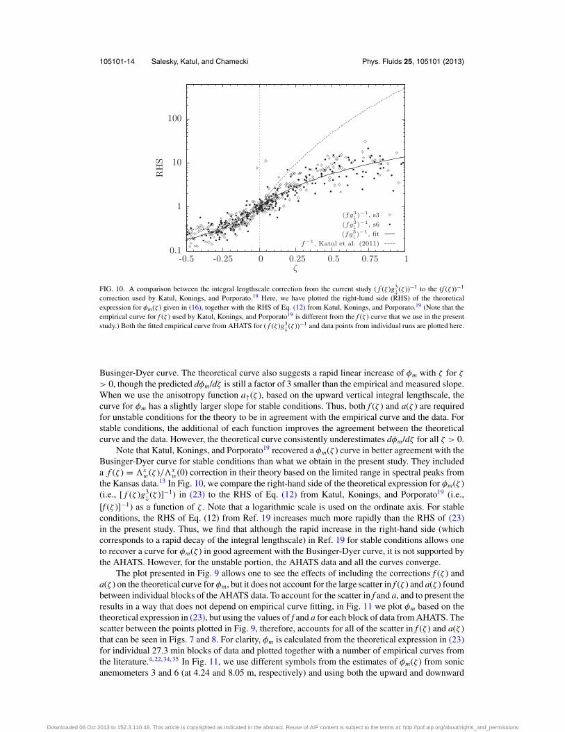
FIG. 10. A comparison between the integral lengthscale correction from the current study ( f (ζ )g3↓(ζ ))−1 to the (f (ζ ))−1

correction used by Katul, Konings, and Porporato.19 Here, we have plotted the right-hand side (RHS) of the theoreticalexpression for φm(ζ ) given in (16), together with the RHS of Eq. (12) from Katul, Konings, and Porporato.19 (Note that theempirical curve for f (ζ ) used by Katul, Konings, and Porporato19 is different from the f (ζ ) curve that we use in the presentstudy.) Both the fitted empirical curve from AHATS for ( f (ζ )g3

↓(ζ ))−1 and data points from individual runs are plotted here.

Businger-Dyer curve. The theoretical curve also suggests a rapid linear increase of φm with ζ for ζ

> 0, though the predicted dφm/dζ is still a factor of 3 smaller than the empirical and measured slope.When we use the anisotropy function a↑(ζ ), based on the upward vertical integral lengthscale, thecurve for φm has a slightly larger slope for stable conditions. Thus, both f (ζ ) and a(ζ ) are requiredfor unstable conditions for the theory to be in agreement with the empirical curve and the data. Forstable conditions, the additional of each function improves the agreement between the theoreticalcurve and the data. However, the theoretical curve consistently underestimates dφm/dζ for all ζ > 0.

Note that Katul, Konings, and Porporato19 recovered a φm(ζ ) curve in better agreement with theBusinger-Dyer curve for stable conditions than what we obtain in the present study. They includeda f (ζ ) = �x

w(ζ )/�xw(0) correction in their theory based on the limited range in spectral peaks from

the Kansas data.13 In Fig. 10, we compare the right-hand side of the theoretical expression for φm(ζ )(i.e., [ f (ζ )g3

↓(ζ )]−1) in (23) to the RHS of Eq. (12) from Katul, Konings, and Porporato19 (i.e.,[f (ζ )]−1) as a function of ζ . Note that a logarithmic scale is used on the ordinate axis. For stableconditions, the RHS of Eq. (12) from Ref. 19 increases much more rapidly than the RHS of (23)in the present study. Thus, we find that although the rapid increase in the right-hand side (whichcorresponds to a rapid decay of the integral lengthscale) in Ref. 19 for stable conditions allows oneto recover a curve for φm(ζ ) in good agreement with the Businger-Dyer curve, it is not supported bythe AHATS. However, for the unstable portion, the AHATS data and all the curves converge.

The plot presented in Fig. 9 allows one to see the effects of including the corrections f (ζ ) anda(ζ ) on the theoretical curve for φm, but it does not account for the large scatter in f (ζ ) and a(ζ ) foundbetween individual blocks of the AHATS data. To account for the scatter in f and a, and to present theresults in a way that does not depend on empirical curve fitting, in Fig. 11 we plot φm based on thetheoretical expression in (23), but using the values of f and a for each block of data from AHATS. Thescatter between the points plotted in Fig. 9, therefore, accounts for all of the scatter in f (ζ ) and a(ζ )that can be seen in Figs. 7 and 8. For clarity, φm is calculated from the theoretical expression in (23)for individual 27.3 min blocks of data and plotted together with a number of empirical curves fromthe literature.4, 22, 34, 35 In Fig. 11, we use different symbols from the estimates of φm(ζ ) from sonicanemometers 3 and 6 (at 4.24 and 8.05 m, respectively) and using both the upward and downward



0

1

2

3

4

5

6

7

-2 -1.5 -1 -0.5 0 0.5 1

φm

(ζ)

ζ

Zilitinkevitch and Tschalikov (1968)Businger-DyerHogstrom (1988)Handorf et al. (1999)s3, a↑(ζ)s3, a↓(ζ)s6, a↓(ζ)

FIG. 11. φm(ζ ) predicted by the theoretical expression in (17), but using values of f and a calculated for individual blocksof data. Several empirical curves from the literature are also shown.

anisotropy function from sonic anemometer 3. In Fig. 11, the empirical curves are generally in goodagreement with each other for unstable conditions, but diverge for stable conditions. The calculatedvalues of φm from the theory are in good agreement with all of the empirical curves for unstableconditions. For stable conditions, however, the values of φm from the theory are consistently smallerthan the empirical curves reported across several experiments. The theory predicts a linear increasein φm for stable conditions, but it still predicts a value of φm smaller than what would be within therange of reported experimental values spanned by the set of empirical curves.

Even though the scatter in φm due to the scatter in f and a from individual blocks of data doeslead to a large spread for stable conditions, this scatter still does not account for the differencesbetween the theoretical φm and the empirical curves observed for the stable cases. It is not entirelyclear what leads to the disagreement between theory and observed values of φm for the stable cases.However, it can be conjectured that the differences are due to physical processes not accounted forin the theoretical model rather than random noise in the estimation of parameters.

E. Approximate solutions for φm(ζ )

The theoretical expression for φm(ζ ) in (23) is an implicit equation, and it, therefore, is notamenable to a general analytical solution. However, it is still desirable to make an explicit connectionbetween the stability variation of the integral scale and eddy anisotropy and the coefficients inempirical curves for φm(ζ ). Because we found good agreement between φm(ζ ) from the theoryand empirical curves for unstable conditions, we here consider approximate solutions for φm(ζ ) forslightly unstable (| − ζ | � 1) and free convective (| − ζ | � 1) conditions in order to make an explicitconnection between the coefficients in empirical φm(ζ ) curves and stability-dependent properties ofturbulence such as the integral scales and eddy anisotropy.

In the slightly unstable case, one can derive an approximate solution to the φm(ζ ) equation in(23) by noting that ζ /φm(ζ ) ≈ ζ , and by expanding f (ζ ) and g(ζ ) in Taylor series about ζ = 0.Appendix B presents details of the derivations. If we retain the linear and quadratic terms in theTaylor series, we find

φm(ζ ) = [1 − (a f b f + 3agbg)ζ + 3(agbg + a f b f agbg + 2a2

gb2g)ζ 2 + O(ζ 3)

]−1/4, (25)

where af, bf, ag, and bg are the coefficients in the curves of the form (24) fit to f (ζ ) and g(ζ ); valuesof these coefficients from the AHATS data can be found in Table I. Thus, (25) explicitly shows



0.1

1

0.010.1110

φm

(ζ)

−ζ

(a)

0.1

1

0.010.1110 −ζ

(b)

0.1

1

0.010.1110 −ζ

(c)

No correctionsBusinger-Dyer

(1 − ζ)−1/4

(−ζ)−1/3

f(ζ) and a↓(ζ)Businger-Dyer(1 − 5.8ζ)−1/4

(1 − 5.8ζ + 19.8ζ2)−1/4

f(ζ) and a↓(ζ)Businger-Dyer0.47(−ζ)−1/3

0.41(−ζ)−1/3

FIG. 12. Numerical solution to (16) for φm(ζ ) (a) without corrections for the integral scale and eddy anisotropy (b) and (c)with corrections (f (ζ ) and a(ζ )) for both of these effects. Panel (a) also shows powerlaw scaling for slightly unstable and freeconvective conditions. In panel (b), we plot the approximate solution for φm(ζ ) for slightly unstable conditions; in panel (c),we show the approximate solution for free convective conditions. Note that a log-log scale is used for all panels.

the link between the coefficients in curves for φm(ζ ) and the f and g functions that account for thestability dependence of the horizontal and vertical integral lengthscales. By introducing the valuesof the empirical coefficients in the f (ζ ) and g↓(ζ ) curves, (25) reduces to

φm(ζ ) ≈ [1 − 5.8ζ + 19.8ζ 2]−1/4

. (26)

Under free convective conditions, we note that −ζ /φm � 1 and observe that both f and g tendtoward constant values, i.e., f (ζ ) → C f and g(ζ ) → Cg as | − ζ | → ∞. Under these assumptions,the approximate solution to (23) is

φm(ζ ) = C−1/3f C−1

g (−ζ )−1/3, (27)

which indicates that the coefficient in (−ζ )−1/3 powerlaw for free convective conditions is linkedto the asymptotic behavior of the horizontal and vertical integral lengthscales in the free convectivelimit. Introducing the values of C f ≈ 1.86 and Cg ≈ 1.72 (for g↓(ζ )) found from the AHATS data,we obtain

φm(ζ ) ≈ 0.47(−ζ )−1/3. (28)

Note that the coefficient of 0.47 here is very close to the value of 0.41 obtained empirically byZilitinkevich and Tschalikov.34 If we use the value of Cg ≈ 2.06 based on g↑(ζ ), we obtain φm(ζ )≈ 0.39( − ζ )−1/3, also in very good agreement with experimental results.

These approximate solutions for φm(ζ ) are plotted in Fig. 12 and are compared with thenumerical solution to (23). As discussed previously, when one neglects stability variation of theintegral lengthscale and eddy anisotropy (i.e., f = a = 1), one can still obtain the scaling laws of(φm ∼ (1 − ζ )−1/4) for slightly unstable conditions and (φm(ζ ) ∼ ( − ζ )−1/3) for free convectiveconditions. Figure 12(a) shows these scalings compared to the theoretical φm(ζ ) curve without thef and a corrections (i.e., for f = a = 1). Note that although the theoretical curve is able to recoverthese scalings, it predicts values of φm(ζ ) larger than the Businger-Dyer curve for the entire unstablerange plotted here.

In Figs. 12(b) and 12(c), we plot the numerically obtained φm(ζ ) curve from (23) when weinclude the corrections for the integral lengthscale (f) and eddy anisotropy (a). Note that (as discussedpreviously) these corrections bring the theoretical φm(ζ ) curve into better agreement with theBusinger-Dyer curve. In panel (b), we show the approximate solution for slightly unstable conditions;in panel (c), we show the approximate solution for free convection. For slightly unstable conditions,we find that retaining only the linear terms in the Taylor series give us φm(ζ ) = (1 − 5.8ζ )−1/4,which is a good approximation to the numerically obtained φm(ζ ) curve for ζ > 0.1. However, if wealso retain the quadratic term in ζ , the approximate solution of φm(ζ ) = [1 − 5.8ζ + 19.8ζ 2]−1/4 isa good representation of the numerical solution for −1 < ζ < 0.



The approximate solution for free convection (i.e., φm(ζ ) = 0.47( − ζ )−1/3) is displayedin panel (c) together with the numerical solution to (23). The approximate solution representsthe numerically obtained curve well for ζ < −2. Another line is plotted in panel (c) for φm(ζ )= 0.41( − ζ )−1/3; Zilitinkevich and Tschalikov34 obtained the coefficient of 0.41 empirically. Notethat the numerically obtained curve for φm(ζ ) and our approximate solution are in better agreementwith Ref. 34 than the Businger-Dyer curve is for ζ < −1, which reinforces that the theoretical modelfor φm is able to capture the behavior of φm in the free convective limit.

V. DISCUSSION

Using data from the AHATS field experiment, the link between the shape of commonly usedempirical functions for the dimensionless mean velocity gradient φm(ζ ) and stability-dependentproperties of turbulence in the ASL (i.e., the integral lengthscale, the anisotropy of the momentum-transporting eddies, and the local imbalance of the TKE budget) was investigated. Several mod-ifications were proposed to the theoretical expression for φm(ζ ) presented in Ref. 19 to accountexplicitly for the stability-dependence of the integral lengthscale and eddy anisotropy. The AHATSdata support the hypothesis that the coefficients in empirical curves for φm(ζ ) are related to varia-tion with stability of the integral lengthscale and the eddy anisotropy. However, we found that theinclusion of a β2(ζ ) correction to account for the local TKE imbalance and a h(ζ ) correction toaccount for departures from inertial range scaling each had a negligible influence on the behaviorof φm(ζ ).

The stability-dependence of the horizontal and vertical integral lengthscales of w were alsoinvestigated. Both the horizontal (�x

w) and the vertical (�zw) integral lengthscales were found to be

largest for unstable conditions and decayed rapidly with increasing stability. For a given stabilityregime, we found a distinct difference between the value of �z↓

w , calculated from downward spatiallags in the autocorrelation, and �z↑

w , calculated from upward spatial lags. The upward verticalintegral scale �z↑

w has a variation with ζ similar to that of the horizontal integral scale �xw, whereas

the downward integral scale �z↓w is consistently smaller, and decays more slowly with increasing

stability. When the autocorrelation is calculated using upward lags, one samples larger values of z,and subsequently larger values of |ζ | = |z/L| (that is, if u∗ and H0 are constant with height, a standardassumption in MOST). This appears to be the reason for the difference between the calculated valuesof �z↓

w and �z↑w . Note that the estimate of the vertical integral lengthscale from the AHATS dataset

is limited by the number of measurement heights in the vertical; �zw was estimated based on an

exponential function fit to the measured vertical autocorrelation function with either 3 or 4 pointsfor downward or upward lags, respectively, for sonic anemometer 3. This limitation motivates futurestudies of the ASL, either from field experiments with measurements at more vertical levels, or usingnumerical simulations to investigate in greater detail the stability dependence of the horizontal andvertical integral lengthscales and connection to the observed behavior of φm(ζ ).

Although the theory developed in Sec. II is based on an elliptical momentum transporting eddyin the x-z plane (characterized by the horizontal and vertical integral lengthscales �x

w and �zw), the

AHATS data indicate that the vertical integral lengthscale of w depends on the direction of the lagthat is used to compute the autocorrelation function, i.e., �z↓

w (based on downward lags) is differentfrom �z↑

w (based on upward lags). In order to account for the effects of the upward and downwardintegral lengthscale simultaneously, one would have to rewrite Eq. (5) in terms of both �z↓

w and �z↑w ,

i.e.,

u2∗ = κτ v(sx )

[u(�z↑

w + z) − u(�z↓w − z)

]. (29)

However, accounting for both �z↑w and �z↓

w would make it difficult to write (29) in terms of dudz , making

the relationship between φm(ζ ) and stability-dependent properties of turbulence (e.g., integral scales,eddy anisotropy) less clear. Although the data do indicate that the momentum transporting eddy maynot be elliptical (and indeed may be inclined relative to the horizontal), it is not straightforward toincorporate both �z↑

w and �z↓w into the theory simultaneously.



As discussed by Katul, Konings, and Porporato,19 the theoretical expression for φm(ζ ) is ableto reproduce the correct scaling laws for φm(ζ )−φm ∼ ζ for stable conditions, φm ∼ (1 − ζ )−1/4 forslightly unstable conditions, and φm ∼ ( − ζ )−1/3 in the free convective limit. (Here, we use freeconvection to refer to the state of the ABL, typically found for | − ζ | > 5, where the production ofTKE is dominated by buoyancy rather than mechanical production, but ∂u/∂z and u∗ remain finite.36

This is in contrast to natural convection, which is also driven by buoyancy, but ∂u/∂z = 0 and u∗= 0.) These scaling laws are directly related to the stability dependence of TKE production in theASL, which is introduced into the eddy turnover velocity scale (9) through the TKE dissipation rateε, when one assumes local balance in the TKE budget. However, the results from the current studyfurther suggest that the coefficients in empirical curves for φm(ζ ) (e.g., the factors of 16 and 5 inthe unstable and stable branches of the Businger-Dyer curve (4), respectively) are linked to the sizeand anisotropy of the ensemble mean momentum transporting eddy, as the addition of the f (ζ ) anda(ζ ) corrections allow one to recover a curve for φm(ζ ) in good agreement with the data for unstableconditions. The unstable coefficient can be linked to the stable one via a smoothness conditionrequiring that dφm/dζ be continuous at ζ = 0. Linearizing the unstable form of the Businger-Dyercurve about ζ = 0 yields φm = 1 + 4ζ , which suggests that the factor 16 of the unstable portion andthe factor 5 of the stable portion of the Businger-Dyer φm are connected. In a recent study for stablystratified flow, van de Wiel et al.37 argued via model results that φm = 1 + αζ , where α = 1/Ric andRic is the critical Richardson number (=0.2) at which turbulence decays due to stable stratification.Thus, the coefficient of 5 for ζ > 0 in the empirical Businger-Dyer curve may also be connected tothe critical Richardson number in the stable ABL. Hence, within the proposed framework here forφm, stability changes in the ensemble mean eddy size seem to span conditions from nearly collapsedturbulence under stable stratification all the way up to free convection under unstable conditions.Although the inclusion of the stability corrections f (ζ ) and a(ζ ) for the integral scale and eddyanisotropy produce a linear increase of φm with ζ for stable conditions, the theoretical expressionfor φm and values of f and a from the AHATS dataset produce values of dφm/dζ smaller (by afactor of 3) than what has been found for experimental data from the ASL. One potential source ofuncertainty in our analysis for stable conditions is the estimate of the vertical integral lengthscale.For stable conditions, the autocorrelation has a limited number of points with finite correlation forthe spatial lags that were used (the possible values of �z are dictated by the vertical sensor spacing).It, therefore, is possible that our estimate of the integral lengthscale is biased for stable conditions.However, this bias alone may not explain all the failures of the model. The stable form of the φm(ζ )curve and the value of dφm/dζ may also be determined by factors in addition to the ζ -dependence ofthe integral lengthscale and eddy anisotropy, but these factors remain elusive to the present theory.

ACKNOWLEDGMENTS

S. T. Salesky and M. Chamecki acknowledge support from the National Science Foundation,Grant No. AGS-0638385. G. G. Katul acknowledges support from the National Science Foundation(Grant Nos. NSF-AGS-1102227 and NSF-EAR-1013339), the U.S. Department of Energy throughthe Office of Biological and Environmental Research (BER) Terrestrial Ecosystem Science (TES)program (Grant No. DE-SC0006967), the U.S. Department of Agriculture (Grant No. 2011-67003-30222), and the Binational Agricultural Research and Development (BARD) fund (Grant No. IS-4374-11C). The AHATS data were collected by NCAR’s Integrated Surface Flux Facility. Theauthors thank the two reviewers for insightful comments on the article.

APPENDIX A: EMPIRICAL CURVES FOR φm(ζ )

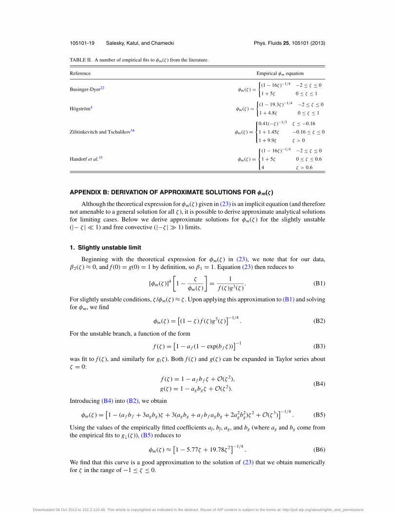
Empirical curves for φm(ζ ) reported from the literature, plotted in Fig. 11, are displayed inTable II. This is not intended to be an exhaustive list, but rather is meant to show the expectedvariations in the functional forms that have been proposed, and differences in the proposed functionsfor stable conditions (ζ > 0).



TABLE II. A number of empirical fits to φm(ζ ) from the literature.

Reference Empirical φm equation

Businger-Dyer22 φm (ζ ) ={

(1 − 16ζ )−1/4 −2 ≤ ζ ≤ 0

1 + 5ζ 0 ≤ ζ ≤ 1

Hogstrom4 φm (ζ ) ={

(1 − 19.3ζ )−1/4 −2 ≤ ζ ≤ 0

1 + 4.8ζ 0 ≤ ζ ≤ 1

Zilitinkevitch and Tschalikov34 φm (ζ ) =

⎧⎪⎨⎪⎩

0.41(−ζ )−1/3 ζ ≤ −0.16

1 + 1.45ζ −0.16 ≤ ζ ≤ 0

1 + 9.9ζ ζ > 0

Handorf et al.35 φm (ζ ) =

⎧⎪⎨⎪⎩

(1 − 16ζ )−1/4 −2 ≤ ζ ≤ 0

1 + 5ζ 0 ≤ ζ ≤ 0.6

4 ζ > 0.6

APPENDIX B: DERIVATION OF APPROXIMATE SOLUTIONS FOR φm(ζ )

Although the theoretical expression for φm(ζ ) given in (23) is an implicit equation (and thereforenot amenable to a general solution for all ζ ), it is possible to derive approximate analytical solutionsfor limiting cases. Below we derive approximate solutions for φm(ζ ) for the slightly unstable(|− ζ | � 1) and free convective (|−ζ | � 1) limits.

1. Slightly unstable limit

Beginning with the theoretical expression for φm(ζ ) in (23), we note that for our data,β2(ζ ) ≈ 0, and f (0) = g(0) = 1 by definition, so β1 = 1. Equation (23) then reduces to

[φm(ζ )]4

[1 − ζ

φm(ζ )

]= 1

f (ζ )g3(ζ ). (B1)

For slightly unstable conditions, ζ /φm(ζ ) ≈ ζ . Upon applying this approximation to (B1) and solvingfor φm, we find

φm(ζ ) = [(1 − ζ ) f (ζ )g3(ζ )

]−1/4. (B2)

For the unstable branch, a function of the form

f (ζ ) = [1 − a f (1 − exp(b f ζ ))

]−1(B3)

was fit to f (ζ ), and similarly for g(ζ ). Both f (ζ ) and g(ζ ) can be expanded in Taylor series aboutζ = 0:

f (ζ ) = 1 − a f b f ζ + O(ζ 2),

g(ζ ) = 1 − agbgζ + O(ζ 2).(B4)

Introducing (B4) into (B2), we obtain

φm(ζ ) = [1 − (a f b f + 3agbg)ζ + 3(agbg + a f b f agbg + 2a2

gb2g)ζ 2 + O(ζ 3)

]−1/4. (B5)

Using the values of the empirically fitted coefficients af, bf, ag, and bg (where ag and bg come fromthe empirical fits to g↓(ζ )), (B5) reduces to

φm(ζ ) ≈ [1 − 5.77ζ + 19.78ζ 2

]−1/4. (B6)

We find that this curve is a good approximation to the solution of (23) that we obtain numericallyfor ζ in the range of −1 ≤ ζ ≤ 0.



2. Free convective limit

In the free convective limit, we note that for large |−ζ |, −ζ /φm � 1. Thus (once again takingβ2(ζ ) ≈ 0) (23) can be reduced to

(−ζ ) [φm(ζ )]3 = 1

f (ζ )g3(ζ ). (B7)

As |−ζ | → ∞, both f (ζ ) and g(ζ ) tend asymptotically toward constant values, i.e., f (ζ ) → C f andg(ζ ) → Cg . Equation (B7) then can be solved for φm to find

φm(ζ ) = C−1/3f C−1

g (−ζ )−1/3. (B8)

Using the values of C f ≈ 1.86 and Cg ≈ 1.72 from AHATS, we find

φm(ζ ) ≈ 0.47(−ζ )−1/3. (B9)

This approximate analytical solution is a good representation to the φm(ζ ) curve obtained from thenumerical solution of (23) for |−ζ | > 2.

1 A. M. Obukhov, “Turbulence in an atmosphere with temperature inhomogeneities,” Tr. Inst. Theor. Geofiz. 1, 95–115(1946).

2 A. S. Monin and A. M. Obukhov, “Turbulent mixing in the atmospheric surface layer,” Tr. Geofiz. Inst. 24, 163–187(1954).

3 J. Businger, J. Wyngaard, Y. Izumi, and E. Bradley, “Flux-profile relationships in the atmospheric surface layer,” J. Atmos.Sci. 28, 181–189 (1971).

4 U. Hogstrom, “Non-dimensional wind and temperature profiles in the atmospheric surface layer: A re-evaluation,” Bound-ary-Layer Meteorol. 42, 55–78 (1988).

5 D. Baldocchi, B. Hincks, and T. Meyers, “Measuring biosphere-atmosphere exchanges of biologically related gases withmicrometeorological methods,” Ecology 69(5), 1331–1340 (1988).

6 J. Moncrieff, R. Valentini, S. Greco, S. Guenther, and P. Ciccioli, “Trace gas exchange over terrestrial ecosystems: methodsand perspectives in micrometeorology,” J. Exp. Bot. 48, 1133 (1997).

7 D. Cline, “Snow surface energy exchanges and snowmelt at a continental, midlatitude alpine site,” Water Resour. Res. 33,689–701, doi:10.1029/97WR00026 (1997).

8 J. Deardorff, “Parameterization of the planetary boundary layer for use in general circulation models,” Mon. Weather Rev.100, 93–106 (1972).

9 J. Louis, “A parametric model of vertical eddy fluxes in the atmosphere,” Boundary-Layer Meteorol. 17, 187–202 (1979).10 A. Beljaars, “The parametrization of surface fluxes in large-scale models under free convection,” Q. J. R. Meteorol. Soc.

121, 255–270 (1995).11 J. Deardorff, “Numerical investigation of neutral and unstable planetary boundary layers,” J. Atmos. Sci. 29, 91–115

(1972).12 C. Moeng, “A large-eddy simulation model for the study of planetary boundary-layer turbulence,” J. Atmos. Sci. 41,

2052–2062 (1984).13 J. Kaimal, J. Wyngaard, Y. Izumi, and O. Cote, “Spectral characteristics of surface-layer turbulence,” Q. J. R. Meteorol.

Soc. 98, 563–589 (1972).14 J. Wyngaard and O. Cote, “The budgets of turbulent kinetic energy and temperature variance in the atmospheric surface

layer,” J. Atmos. Sci. 28, 190–201 (1971).15 P. Frenzen and C. Vogel, “The turbulent kinetic energy budget in the atmospheric surface layer: A review and an experimental

reexamination in the field,” Boundary-Layer Meteorol. 60, 49–76 (1992).16 P. Frenzen and C. Vogel, “Further studies of atmospheric turbulence in layers near the surface: Scaling the TKE budget

above the roughness sublayer,” Boundary-Layer Meteorol. 99, 173–206 (2001).17 X. Li, N. Zimmerman, and M. Princevac, “Local imbalance of turbulent kinetic energy in the surface layer,” Boundary-Layer

Meteorol. 129, 115–136 (2008).18 P. Sullivan, T. Horst, D. Lenschow, C. Moeng, and J. Weil, “Structure of subfilter-scale fluxes in the atmospheric surface

layer with application to large-eddy simulation modelling,” J. Fluid Mech. 482, 101–139 (2003).19 G. Katul, A. Konings, and A. Porporato, “Mean velocity profile in a sheared and thermally stratified atmospheric boundary

layer,” Phys. Rev. Lett. 107, 268502 (2011).20 G. Gioia, N. Guttenberg, N. Goldenfeld, and P. Chakraborty, “Spectral theory of the turbulent mean-velocity profile,” Phys.

Rev. Lett. 105, 184501 (2010).21 J. Businger and A. Yaglom, “Introduction to Obukhov’s paper on ‘turbulence in an atmosphere with a non-uniform

temperature’,” Boundary-Layer Meteorol. 2, 3–6 (1971).22 A. Dyer, “A review of flux-profile relationships,” Boundary-Layer Meteorol. 7, 363–372 (1974).23 R. Adrian, C. Meinhart, and C. Tomkins, “Vortex organization in the outer region of the turbulent boundary layer,” J. Fluid

Mech. 422, 1–54 (2000).24 R. Adrian, “Hairpin vortex organization in wall turbulence,” Phys. Fluids 19, 041301 (2007).25 A. Townsend, The Structure of Turbulent Shear Flow (Cambridge University Press, 1976), p. 429.26 U. Frisch, Turbulence: The Legacy of A. N. Kolmogorov (Cambridge University Press, 1995), p. 296.


http://dx.doi.org/10.1175/1520-0469(1971)028<0181:FPRITA>2.0.CO;2

http://dx.doi.org/10.1175/1520-0469(1971)028<0181:FPRITA>2.0.CO;2

http://dx.doi.org/10.1007/BF00119875

http://dx.doi.org/10.1007/BF00119875

http://dx.doi.org/10.2307/1941631

http://dx.doi.org/10.1093/jxb/48.5.1133

http://dx.doi.org/10.1029/97WR00026

http://dx.doi.org/10.1175/1520-0493(1972)100<0093:POTPBL>2.3.CO;2

http://dx.doi.org/10.1007/BF00117978

http://dx.doi.org/10.1002/qj.49712152203

http://dx.doi.org/10.1175/1520-0469(1972)029<0091:NIONAU>2.0.CO;2

http://dx.doi.org/10.1175/1520-0469(1984)041<2052:ALESMF>2.0.CO;2

http://dx.doi.org/10.1002/qj.49709841707

http://dx.doi.org/10.1002/qj.49709841707

http://dx.doi.org/10.1175/1520-0469(1971)028<0190:TBOTKE>2.0.CO;2

http://dx.doi.org/10.1007/BF00122061

http://dx.doi.org/10.1023/A:1018956931957

http://dx.doi.org/10.1007/s10546-008-9304-z

http://dx.doi.org/10.1007/s10546-008-9304-z

http://dx.doi.org/10.1017/S0022112003004099

http://dx.doi.org/10.1103/PhysRevLett.107.268502



http://dx.doi.org/10.1007/BF00718084

http://dx.doi.org/10.1007/BF00240838

http://dx.doi.org/10.1017/S0022112000001580

http://dx.doi.org/10.1017/S0022112000001580

http://dx.doi.org/10.1063/1.2717527


27 J. C. Kaimal and J. J. Finnigan, Atmospheric Boundary Layer Flows: Their Structure and Measurement (Oxford UniversityPress, 1994), p. 289.

28 X. Lee, W. Massman, and B. Law, Handbook of Micrometeorology: A Guide for Surface Flux Measurement and Analysis(Springer, 2004), p. 264.

29 D. Vickers and L. Mahrt, “Quality control and flux sampling problems for tower and aircraft data,” J. Atmos. Ocean.Technol. 14, 512–526 (1997).

30 M. Chamecki and N. Dias, “The local isotropy hypothesis and the turbulent kinetic energy dissipation rate in the atmosphericsurface layer,” Q. J. R. Meteorol. Soc. 130, 2733–2752 (2004).

31 C. Hsieh and G. Katul, “Dissipation methods, Taylor’s hypothesis, and stability correction functions in the atmosphericsurface layer,” J. Geophys. Res. 102, 16391–16405, doi:10.1029/97JD00200 (1997).

32 J. Wyngaard and S. Clifford, “Taylor’s hypothesis and high-frequency turbulence spectra,” J. Atmos. Sci. 34, 922–929(1977).

33 S. Salesky and M. Chamecki, “Random errors in turbulence measurements in the atmospheric surface layer: implicationsfor Monin-Obukhov similarity theory,” J. Atmos. Sci. 69, 3700–3714 (2012).

34 S. Zilitinkevich and D. Tschalikov, “Determination of universal profiles of wind velocity and temperature in the surfacelayer of the atmosphere,” Izv., Atmos. Oceanic Phys. 4, 249–302 (1968).

35 D. Handorf, T. Foken, and C. Kottmeier, “The stable atmospheric boundary layer over an Antarctic ice sheet,” Bound-ary-Layer Meteorol. 91, 165–189 (1999).

36 B. Kader and A. Yaglom, “Mean fields and fluctuation moments in unstably stratified turbulent boundary layers,” J. FluidMech. 212, 637–662 (1990).

37 B. van de Wiel, A. Moene, G. Steeneveld, O. Hartogensis, and A. Holtslag, “Predicting the collapse of turbulence in stablystratified boundary layers,” Flow, Turbul. Combust. 79, 251–274 (2007).


http://dx.doi.org/10.1175/1520-0426(1997)014<0512:QCAFSP>2.0.CO;2

http://dx.doi.org/10.1175/1520-0426(1997)014<0512:QCAFSP>2.0.CO;2

http://dx.doi.org/10.1256/qj.03.155

http://dx.doi.org/10.1029/97JD00200

http://dx.doi.org/10.1175/1520-0469(1977)034<0922:THAHTS>2.0.CO;2

http://dx.doi.org/10.1175/JAS-D-12-096.1

http://dx.doi.org/10.1023/A:1001889423449

http://dx.doi.org/10.1023/A:1001889423449

http://dx.doi.org/10.1017/S0022112090002129

http://dx.doi.org/10.1017/S0022112090002129

http://dx.doi.org/10.1007/s10494-007-9094-2

Documents

Buoyancy effects on the integral lengthscales and mean