Built-in Self-test

October 26, 2011 1

Introduction

• Test generation and response evaluation done on-chip.

• Only a few external pins to control BIST operation.

• Additional hardware overhead.

October 26, 2011 2

• Additional hardware overhead.

• Offers a number of benefits.

BIST Motivation

• Useful for field test and diagnosis:

– Less expensive than a local automatic test equipment

• Software tests for field test and diagnosis:

– Low hardware fault coverage

– Low diagnostic resolution

– Slow to operate

October 26, 2011 3

– Slow to operate

• Hardware BIST benefits:

– Lower system test effort

– Improved system maintenance and repair

– Improved component repair

– Better diagnosis

Test Generator

Circuit Under Test

BIST – Basic Idea

CHIP

Circuit Under Test(CUT)

Response Compressor

BIST Basics

BIST Architecture

CircuitMU

PatternGenerator

Response

ROM

=

TEST CONTROLLERTEST

October 26, 2011 5

Circuitundertest

UX

Generator

PI

ResponseCompactor =

Good / BadPO

� Note: BIST cannot test wires and transistors:

� From PI pins to input MUX

� From POs to output pins

BIST Costs

– Chip area overhead for:

• Test controller

• Hardware pattern generator / response compactor

• Testing of BIST hardware

– Pin overhead

• At least 1 pin needed to activate BIST operation

– Performance overhead

October 26, 2011 6

– Performance overhead

• Extra path delays due to BIST

– Yield loss

• Due to increased chip area

– Reliability reduction

• Due to increased area

– Increased BIST hardware complexity

• Happens when BIST hardware is made testable

BIST Benefits

• Faults tested:

– Single combinational / sequential stuck-at faults

– Delay faults

– Single stuck-at faults in BIST hardware

• BIST benefits

– Reduced testing and maintenance cost

October 26, 2011 7

– Reduced testing and maintenance cost

– Lower test generation cost

– Reduced storage / maintenance of test patterns

– Simpler and less expensive ATE

– Can test many units in parallel

– Shorter test application times

– Can test at functional system speed

BIST Techniques

• Stored Vector Based

– Microinstruction support

– Stored in ROM

• Algorithmic Hardware Test Pattern GeneratorsGenerators

– Counter :: exhaustive, pseudo-exhaustive

– Linear Feedback Shift Register

– Cellular Automata

BIST Basics - LFSR

Exhaustive Pattern Generation

• Shows that every state and transition works

• For n-input circuits, requires all 2n vectors

• Impractical for n > 20

October 26, 2011 9

Pseudo-Exhaustive Method

• Partition large circuit into fanin cones

– Backtrace from each PO to PIs influencing it

– Test fanin cones in parallel

• An illustrative example (next slide):

– No. of tests reduced from 28 = 256 to 25 x 2 = 64

October 26, 2011 10

– No. of tests reduced from 28 = 256 to 25 x 2 = 64

Pseudo-Exhaustive Pattern Generation

October 26, 2011 11

Random Pattern Testing

• Generate pseudo-random patterns as test input vectors.

• Evaluate fault coverage through fault simulation.

• Motivation:

October 26, 2011 12

• Motivation:– Test length may be larger.

– Faster test generation.

• Used to get tests for 60-80% of faults, then switch to ATPG for rest.

• Some circuits may be random pattern resistant.

%

100%

October 26, 2011 13

Number of test vectors

Fault

Coverage

P R P G

October 26, 2011 14

C U T

Response Evaluation

Linear Feedback Shift Register (LFSR)

October 26, 2011 15

What is LFSR?

• A simple hardware structure based on shift register.

– Linear feedback circuit.

• Has a number of useful applications:

– Pseudo-random number generation

October 26, 2011 16

– Pseudo-random number generation

– Response compression

– Error checking (Cyclic Redundancy Code)

– Data compression

Two types of LFSR

D1 D2 D3 D4

+

Type 1

D1 D2 D4+

Type 2

D3

• Unit delay

– D Flip flop

• Modulo 2 adder

– XOR gate

• Modulo 2 multiplier

– Connection

General Type-1 LFSR

October 26, 2011 18

LFSR Example

1 0 0 00 0 0 10 0 1 10 1 1 11 1 1 11 1 1 01 1 0 1

4 D D2 D1D3

+

D4D3D2D1

1)( 14 ++= xxxf

1 1 0 11 0 1 00 1 0 11 0 1 10 1 1 01 1 0 01 0 0 10 0 1 00 1 0 01 0 0 0

LFSR - Recurrence Relation

...

DnDn-1D2 D3D1

gn-1

+

g2

+

g1

+

...

Is a-1 a-2 a-3 ... a-n+1 a-n

• Generating Function

• Characteristic polynomial

G x a xmm

m( ) ==

∞

∑0

f x c xii

i

n

( ) ==

∑1

Is a-1 a-2 a-3 ... a-n+1 a-n

Cs am-1 am-2 am-3 ... am-n+1 am-n

+ 1

LFSR - Recurrence Relation (continue)

G(x)∞

m=0= ∑ am x

m

= ∑ ∑ ci am-i xm = ∑ ci x

i ∑ am-i xm-i

m=0

∞

i =1

n

m=0

∞

i =1

n

am = ∑ ci am-ii =1

n

= ∑ ∑ ci am-i x = ∑ ci x ∑ am-i x

= ∑ ci xi [a-i x

-i +...+ a-1 x-1 + ∑am x

m]

= ∑ ci xi [a-i x

-i +...+ a-1 x -1 + G(x)]

m=0 i =1

i =1

n

m=0i =1

m=0

∞

i =1

n

LFSR - Recurrence Relation (continue)

( )

( )

1

)(

)()(

1

1

1

1

1

1

1

xc

xaxaxc

xG

xaxaxcxGxcxG

ni

i

n

i

i

i

i

i

n

i

i

i

i

i

n

i

i

i

+

++

=⇒

+++=⇒

=

=

−

−

−

−

=

−

−

−

−

=

∑

∑

∑∑

L

L

( )

)(

1)( 1 and 0 if

)()(

121

1

1

1

1

xfxGaaaa

xf

xaxaxc

xG

nn

n

i

i

i

i

i

i

=⇒=====

++

=

−+−−−

=

−

−

−

−

=

∑

∑

L

L

G(x) is function of initial state and g(x)

LFSR - Definitions

• If the sequence generated by an n-stage LFSR has period 2n-1, then it is called a maximum-length sequence or m-sequence.

• The characteristic polynomial associated with maximum-length sequence is called a with maximum-length sequence is called a primitive polynomial.

• An irreducible polynomial is one that cannot be factored; i.e., it is not divisible by any other polynomial other than 1 and itself.

Example Primitive Polynomials

3: 1 0 ���� x3 + x + 1

4: 1 0

5: 2 0

6: 1 0

October 26, 2011 24

7: 1 0

8: 6 5 1 0

16: 5 3 2 0

32: 28 27 1 0

64: 4 3 1 0

LFSR - Theories

• If the initial state of an LFSR is

a-1 = a-2 = ... = a1-n = 0, a-n = 1

then the LFSR sequence {am} is periodic with a period that is the smallest integer k for which f(x) divides (1+xk).

• An irreducible polynomial f(x) satisfying the following • An irreducible polynomial f(x) satisfying the following two conditions is a primitive polynomial:

– It has an odd number of terms including the 1 term.

– If its degree n is greater than 3, then f(x) must divide (1 + xk), where k = 2n–1

BIST Basics - LFSR

Properties of m-sequences

1. The period of {an} is p=2n-1, that is, ap+I = ai, for all i ≥≥≥≥ 0.

2. Starting from any nonzero state, the LFSR that generates {an} goes through all 2n-1 states before repeating.

3. The number of 1’s differs from the number of 0’s by

October 26, 2011 26

3. The number of 1’s differs from the number of 0’s by one.

4. If a window of width n is slid along an m-sequence, then each of the 2n-1 nonzero binary n-tuples is seen exactly once in a period.

5. In every period of an m-sequence, one-half the runs have length 1, one-fourth have length 2, one-eighth have length 3, and so on.

Randomness Properties of m-sequence

• m-sequences generated by LFSRs are called pseudo random sequence.

– The autocorrelation of any output bit is very close to zero.

– The correlation of any two output bits is very – The correlation of any two output bits is very close to zero.

BIST Basics - LFSR

LFSR as Pseudo-Random Pattern Generator

• Standard LFSR

– Produces patterns algorithmically – repeatable.

– Has most of desirable randomness properties.

• Need not cover all 2n input combinations.

• Long sequences needed for good fault

October 26, 2011 28

• Long sequences needed for good fault coverage.

Weighted Pseudo-Random Pattern Generation

• If p (1) at all PIs is 0.5, pF (1) = 0.58 =1

256

F

s-a-0

October 26, 2011 29

• If p (1) at all PIs is 0.5, pF (1) = 0.5 =

• Will need enormous # of random patterns to test a stuck-at 0 fault on F.

• We must not use an ordinary LFSR to test this.

• IBM holds patents on weighted pseudo-random pattern generator in ATE.

256

255256

1256

pF (0) = 1 – =

• LFSR p (1) = 0.5

• Solution: – Add programmable weight selection and

complement LFSR bits to get p (1)’s other than 0.5.

October 26, 2011 30

0.5.

• Need 2-3 weight sets for a typical circuit.

• Weighted pattern generator drastically shortens pattern length for pseudo-random patterns.

Weighted Pattern Generator

October 26, 2011 31

w1

0

0

0

0

w2

0

0

1

1

Inv.

0

1

0

1

p (output)

½

½

¼

3/4

w1

1

1

1

1

w2

0

0

1

1

p (output)

1/8

7/8

1/16

15/16

Inv.

0

1

0

1

How to compute weights?

• Assume p(1) of primary output(s) to be 0.5.

• Systematically backtrace and compute the p(1) values of all other lines.

• Finally obtain the p(1) values of the

October 26, 2011 32

• Finally obtain the p(1) values of the primary input lines.

Cellular Automata (CA)

• Superior to LFSR – even “more” random

� No shift-induced bit value correlation

� Can make LFSR more random with linear phase shifter

• Regular connections – each cell only connects to local neighbors

xc-1 (t) xc (t) xc+1 (t)

October 26, 2011 33

xc-1 (t) xc (t) xc+1 (t)

Gives CA cell connections

111 110 101 100 011 010 001 000

xc (t + 1) 0 1 0 1 1 0 1 0

26 + 24 + 23 + 21 = 90 Called Rule 90

xc (t + 1) = xc-1 (t) ⊕⊕⊕⊕ xc+1 (t)

Cellular Automata Example

October 26, 2011 34

• Five-stage hybrid cellular automaton

• Rule 150: xc (t + 1) = xc-1 (t) ⊕⊕⊕⊕ xc (t) ⊕⊕⊕⊕ xc+1 (t)

• Alternate Rule 90 and Rule 150 CA

Test Pattern Augmentation

• Secondary ROM – to get LFSR to 100% stuck-at fault coverage.

– Add a small ROM with missing test patterns.

– Add extra circuit mode to input MUX – shift to ROM patterns after LFSR done.

– LFSR reseeding is another alternative.

October 26, 2011 35

– LFSR reseeding is another alternative.

• Use diffracter:

– Generates cluster of patterns in neighborhood of stored ROM pattern.

• Transform LFSR patterns into new vector set.

• Put LFSR and transformation hardware in full-scan chain.

Test Response Compaction

October 26, 2011 36

Response Compaction

• Huge volume of data in CUT response:

– An example:

• Generate 5 million random patterns

• CUT has 200 outputs

• Leads to: 5 million x 200 = 1 billion bits response

October 26, 2011 37

• Uneconomical to store and check all of these responses on chip.

• Responses must be compacted.

Definitions

• Aliasing

– Due to information loss, signatures of good and some bad circuits match.

• Compaction

– Drastically reduce # bits in original circuit

October 26, 2011 38

– Drastically reduce # bits in original circuit response.

– Loss of information.

• Compression

– Reduce # bits in original circuit response .

– No information loss – fully invertible (can get back original response).

• Signature analysis

– Compact good machine response into good machine signature.

– Actual signature generated during testing, and compared with good machine signature

October 26, 2011 39

compared with good machine signature

• Ones Count (Syndrome) Compaction.

– Count # of 1’s

• Transition Count Response Compaction

– Count # of transitions from 0 ���� 1 and 1 ���� 0

as a signature.

BIST - Response Compression

• Introduction

• Ones-Count Compression

• Transition-Count Compression

• Syndrome-Count Compression

• Signature Analysis

• Space Compression

Some Points

• Bit-to-bit comparison is infeasible for BIST.

• General principle:

– Compress a very long output sequence into a single signature.

– Compare the compressed word with the prestored golden signature to determine the correctness of the

October 26, 2011 41

golden signature to determine the correctness of the circuit.

• Problem of aliasing:

– Many output sequences may have the same signature after the compression.

• Poor diagnosis resolution after compression.

Ones-Count - Hardware

• Apply predetermined patterns.

• Count the number of ones in the output sequence.

TestTest

PatternCUT

CounterClock

Ones Counter - Aliasing

• Aliasing Probability

m : the test length

[ ]( ) 2

1

12

1mP

m

m

rOC π≅

−

−=

m : the test lengthr : the number of ones

• r=m/2 :: the case with the highest aliasing prob.

• r=m and r=0 :: no aliasing probability

• For combinational circuits, the input sequence can be permuted without changing the count.

Transition Count - Hardware

• Apply predetermined patterns

• Count the number of the transitions(0 ����1 and 1 ���� 0).

DFF

Test

PatternCUT

CounterClock

DFF

Transition Count

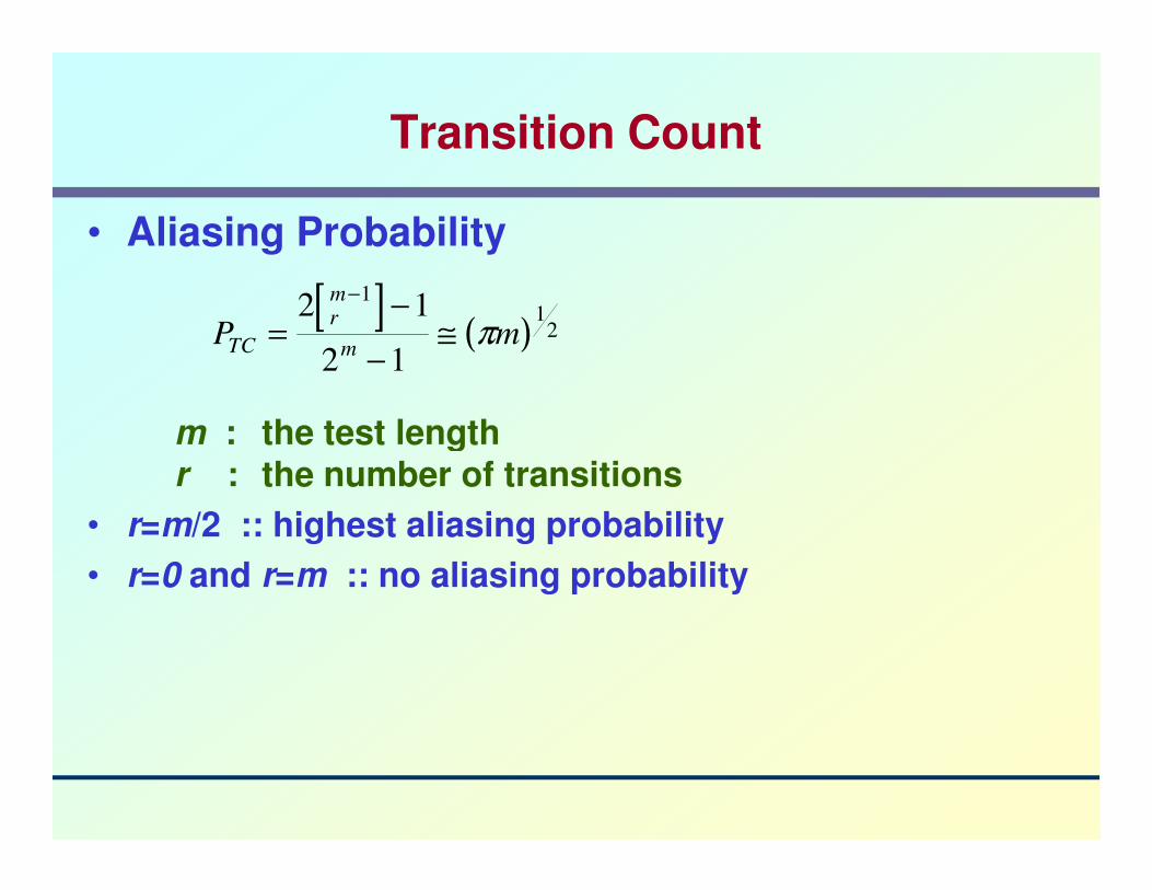
• Aliasing Probability

m : the test length

[ ]( )P mTC

rm

m=

−

−≅

−2 1

2 1

11

2π

m : the test lengthr : the number of transitions

• r=m/2 :: highest aliasing probability

• r=0 and r=m :: no aliasing probability

� Transition count:

C (R) = ΣΣΣΣ (ri ⊕⊕⊕⊕ ri-1) for all m primary outputsi = 1

m

October 26, 2011 46

� To maximize fault coverage:

� Make C (R0) – good machine transition count –as large or as small as possible

Syndrome Testing

• Apply exhaustive test patterns.

• Count the number of 1’s in the output.

• Normalize by dividing with number of minterms.

counter CUT

Syndrome counterClock

Analysis of Syndrome Testing

October 26, 2011 48

Signature Analysis

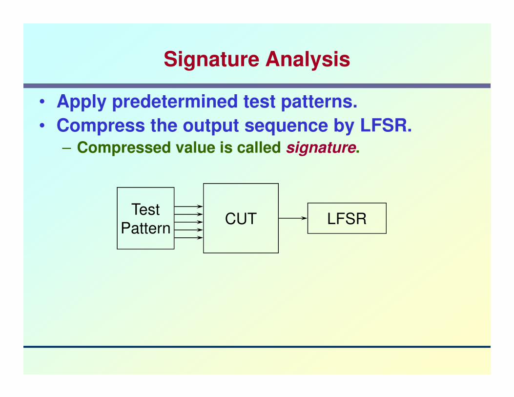
• Apply predetermined test patterns.

• Compress the output sequence by LFSR.– Compressed value is called signature.

Test

PatternCUT LFSR

Signature Analysis

• Aliasing Probability

m: test length, n: length of LFSR

• Aliasing probability is output independent.

PSA

m n

m

n=

−

−≅

−−2 1

2 12

• Aliasing probability is output independent.

• An LFSR with two or more nonzero coefficients detect any single faults.

• An LFSR with primitive polynomial detect any double faults separated less than 2n-1.

LFSR Based Response Compaction

October 26, 2011 51

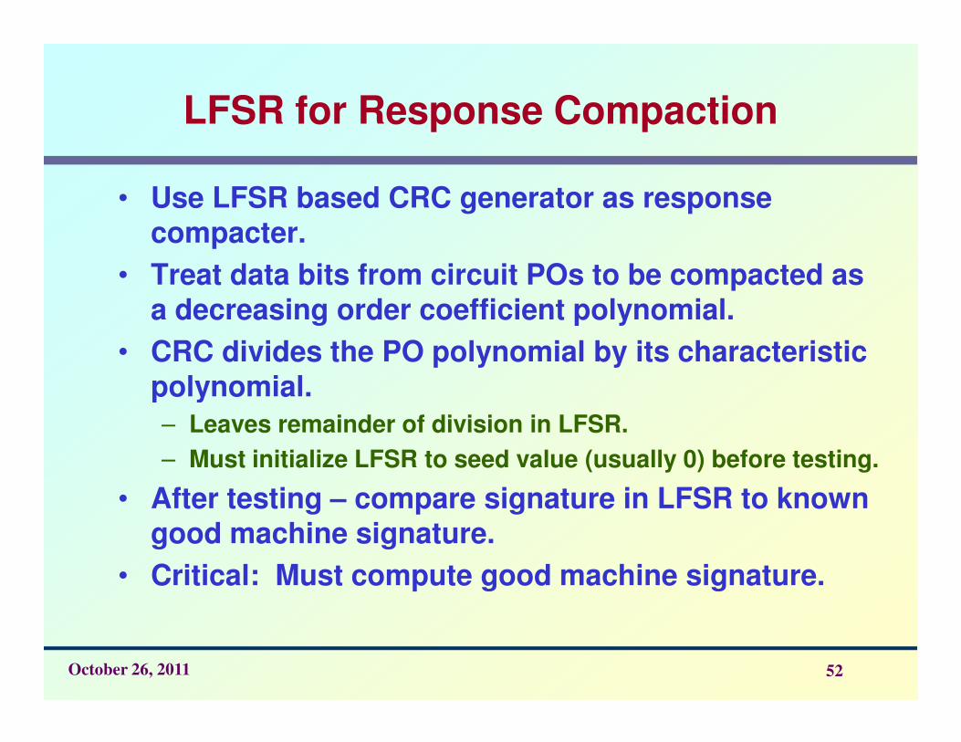
LFSR for Response Compaction

• Use LFSR based CRC generator as response compacter.

• Treat data bits from circuit POs to be compacted as a decreasing order coefficient polynomial.

• CRC divides the PO polynomial by its characteristic polynomial.

October 26, 2011 52

polynomial.

– Leaves remainder of division in LFSR.

– Must initialize LFSR to seed value (usually 0) before testing.

• After testing – compare signature in LFSR to known good machine signature.

• Critical: Must compute good machine signature.

Example Modular LFSR Response Compacter

October 26, 2011 53

• LFSR seed value is “00000”

Polynomial Division

InputsInitial State

1000

X0

01000

X1

00100

X2

00010

X3

00001

X4

00000

LogicSimulation:

October 26, 2011 54

Logic simulation: Remainder = 1 + x2 + x3

0 1 0 1 0 0 0 1

Input polynomial: x1 + x3 + x7

01010

01111

00010

00001

10101

01010

Simulation:

Symbolic Polynomial Division

x2

x7

x7

+ 1

+ x5

x5

+ x3

+ x3 + x2

+ x2

+ x

+ x

x5 + x3 + x + 1

October 26, 2011 55

x

x5 + x3

x3

+ x

+ x2

+ x

+ x + 1

+ 1remainder

Remainder matches that from logic simulationof the response compacter!

Multiple-Input Signature Register (MISR)

• Problem with ordinary LFSR response compacter:– Too much hardware if one of these is put on

each primary output (PO)

• Solution: MISR – compacts all outputs into one LFSR

October 26, 2011 56

one LFSR– Works because LFSR is linear – obeys

superposition principle

– Superimpose all responses in one LFSR

– Final remainder is XOR sum of remainders of polynomial divisions of each PO by the characteristic polynomial

Multiple Input Signature Register (MISR)

type 1

D4 + D3 + D2 + D1 +

+

D4 + D3 + D2 + D1 +

type 2

type 1

MISR Matrix Equation

• di (t) – output response on POi at time t

X0 (t + 1) 10

0… 0 0 X0 (t) d0 (t)

October 26, 2011 58

X0 (t + 1)X1 (t + 1)

.

.

.Xn-3 (t + 1)Xn-2 (t + 1)Xn-1 (t + 1)

10...00

h1

0...0

0

1

…

…

…

…

…

00...10

hn-2

00...01

hn-1

X0 (t)X1 (t).

.

.Xn-3 (t)Xn-2 (t)Xn-1 (t)

=

d0 (t)d1 (t).

.

.dn-3 (t)dn-2 (t)dn-1 (t)

+

Modular MISR Example

October 26, 2011 59

X0 (t + 1)X1 (t + 1)X2 (t + 1)

001

010

110

=

X0 (t)X1 (t)X2 (t)

d0 (t)d1 (t)d2 (t)

+

Multiple Signature Checking

• Use 2 different testing epochs:

� 1st with MISR with 1 polynomial

� 2nd with MISR with different polynomial

• Reduces probability of aliasing –

� Very unlikely that both polynomials will alias for the same

October 26, 2011 60

� Very unlikely that both polynomials will alias for the same fault

• Low hardware cost:

� A few XOR gates for the 2nd MISR polynomial

� A 2-1 MUX to select between two feedback polynomials

Summary

• LFSR pattern generator and MISR response compacter – preferred BIST methods

• BIST has overheads: test controller, extra circuit delay, Input MUX, pattern generator, response compacter, DFT to initialize circuit & test the test hardware

October 26, 2011 61

hardware

• BIST benefits:– At-speed testing for delay & stuck-at faults

– Drastic ATE cost reduction

– Field test capability

– Faster diagnosis during system test

– Less effort to design testing process

– Shorter test application times