BUILDING SYNTHETIC SOCIAL NETWORKS USING ASSOCIATION …

56

BUILDING SYNTHETIC SOCIAL NETWORKS USING ASSOCIATION

RULES AND CLUSTERING METHODS: CASE STUDY ON GLOBAL

TERRORISM DATABASE

Jan Górecki1, Kateřina Slaninová

2

1 Slezská univerzita, Obchodně podnikatelská fakulta, Univerzitní nám. 1934/3, 733 40 Karviná

Email:[email protected]

2 Slezská univerzita, Obchodně podnikatelská fakulta, Univerzitní nám. 1934/3, 733 40 Karviná

Email: [email protected]

Abstract: The authors of the paper present an approach for datamining methods combination (method

for association rules extraction and clustering method are combined) which is used for synthetic social

networks construction which afterwards represents potentially interesting relations in analyzed data.

Described approach is feasible for general data, principles of described approach, examples and

experiments are illustrated on a part of unique database, which contain data about terroristic attack

committed on all over the World (Global Terrorism Database). Thus this paper also extend framework

of papers focused on analysis of this unique database.

Keywords: association rules, community analysis, graph visualization, synthetic social network.

JEL classification: C38, Z00

Doručeno redakci: 22.6.2012; Recenzováno: 13.3.2013; 10.3.2013; Schváleno k publikování: 19.6.2013

Introduction

Data mining techniques like clustering methods and association rule mining methods are

methods for the analysis of observational data sets used to find unsuspected relationships and

to summarize the data in novel ways that are both understandable and useful to the data owner

(Hand, 2001). Data mining is commonly a multistage process of extracting previously

unanticipated knowledge from large data collections, and applying the results to decision

making (Benoît, 2002). Data mining tools are able to detect patterns from the data and infer

associations and rules from them. The development and the fundamental methods of the

social network visualization were published by Freeman (2004). The extracted information

can be applied in the prediction process or for construction of classification models using the

relations within the data records or between the data collections. Those patterns, in Social

network analysis, can be represented as patterns of groups (or communities) in social network

structure and can then guide the network visualization and the study of network evolution.

This type of information can be valuable in the decision making process and forecast the

effects of those decisions.

The main purpose or the paper is to model synthetic social network based on relations

obtained from the data collection about terroristic incidents to found new, often latent or

unexpected characteristics and patterns of the data. The social network is constructed under

the information obtained using two data mining techniques - association rules mining and

clustering. Discovered relations based on the similar behavior were analyzed and visualized

using the methods of graph theory. The latent ties in the social network were represented by

the level of similarity of the objects, which was computed from the attribute analysis

performed on the previous data mining level.

57

For the analysis was used the Global Terrorism Database (GTD) produced by the National

Consortium for the Study of Terrorism and Responses to Terrorism (START)1. There were

published several works oriented to the visualization of the information obtained from GTD

and some of them will be described in next chapter.

1 Related work

First analytical tool you probably meet while you start to interest in GTD is accessible on-line

right on website of START and is called GTD Data Rivers (Lee, 2008). This web-based

interactive exploratory tool provides aggregation of important variables from the database and

visualization of results as comprehensible stack charts, what provides quick and easy insight

to the data for experts with no need of downloading any special analytical software.

Next visualization system with focus on GTD offers more complex possibilities for visual

explorations and it consists of three interlinked components with different complementary

perspectives on the data – investigation, projection and exploration (Godwin, 2008), (Jones,

2008), (Kosara, 2006), (Wang, 2008). Illustration of these three components can be seen on

Figure 1.

Figure 1: Three components of visualization system: Investigation, Projection and

Exploration

Source: Godwin (2008), Jones (2008), Kosara (2006), Wang (2008).

First component, (Jones, 2008), (Wang, 2008) ,offers Investigative view which is focused on

investigation in geotemporal context built around basic questions who, what, when and where.

Second component, (Godwin, 2008), can be used to detailed investigation of temporal

patterns and is based on methods successfully used in biometrics, particularly in longest

common subsequence analysis of sequences of nucleotides. Methods for gene analysis were

adjusted for data structure of GTD using sequences of attacks of terrorist groups instead of

sequences in genes for comparison, so the component offers the comparison of the behavior

of two logical groupings of terrorist’s events as it changes over time – in this place we have to

note that the term “behavior” has the quite different meaning that meaning as we use it in this

work in the text below.

1 Global Terrorism Database, START, accessed on 30 January 2011

58

Third component (Kosara, 2006) supports exploration of relationships among dimensions in

more abstract manner than previous two components. This component shows degree of

correlation between categorical dimensions (attributes) using “ribbons” that are sized based

on the number of cases two categories share. This component is very illustrative for smaller

amount of categories and is very useful while focused on specific small subset of groups

(categories), which we want to analyze. But in case of large amount of categories (in GTD

there are for example more than thousand of different terroristic groups, hundreds of countries

where attacks are committed), may happen to be almost impossible to get comprehensible

visualization. It’s also possible to explore with this tool relations among categories of more

than two attributes (dimensions), but with multiplying number of categories from all

dimensions it brings another difficulty in understanding of visualizations. To solve this

problem with large amount of categories (in case of composition of multiple dimensions from

data referred as “The Curse of Dimensionality” (Zhang, 2009)) we created method, that filter

very effectively data preserving only interesting or important (captured by what we call

“typical behavior” described later in text) relations in data, what (that interestingness or

importance) can be defined by mean of some tunable parameters for filtering in selected data

mining method. Filtered data are then presented graphically in synthetic social network for

further visual investigation (you can see example on Figure 2).

Source: own.

Moreover, using datamining paradigm that we want answers not only on what we have

questioned but also what we have not – revealing interesting answers for questions which do

not ordinarily come on mind, we can discover unexpected similarities among different

terroristic groups. So, our method can serve in a first step for investigating interesting

similarities among all terroristic groups in GTD and then in second step focusing on some

community (group of terroristic groups) can be investigated more specifically similarities (or

vice versa differences) among them by means of above mentioned methods.

2 Typical behavior analysis

Our intention is to extend visualization system mentioned in previous section with next

complementary tool for visualization of all the information in GTD by means of what we call

“typical behavior” of individual terroristic groups and present it graphically in synthetic social

network, what can serve as first step of exploration of GTD in global scope and after this step,

when we have analyzed interesting similarities among all terroristic groups in the data, we can

continue with exploration of the data in more specific focus (as mentioned before). In the first

Figure 2: Graph of Synthetic Social Network

59

subsection we formally define what we mean by the expression behavior and in the second

subsection we discuss the mean of the adjective typical.

2.1 Behavior

Suppose we have data D(o,X) in general form

Table 1: General form of data matrix

X1 … Xn

o(1)

)1(

1x … )1(

nx

o(j)

… )( j

ix …

o(m)

)(

1

mx … )(m

nx

Source: own. where:

1) o = {o(1)

,…,o(m)

} is set of some objects (processes, transactions, etc.),

2) X = {X1,…,Xn} is set of variables (attributes),

3) )( j

ix are values of ith attribute measured on jth object, formally2 ii nX

o: is mapping

defined as mjnixoX i

j

i

j

i

,,)( )()(

(we do not restrict in

to be a set of natural

numbers – it can be any finite set of categories as every set of categories can be

mapped to a set of natural number – we use in

just for simplification of notation)3.

This general form has also data from GTD, whose sample is illustrated in Table 2 and we use

this sample for all examples in text below.

To form groups of objects which we want to compare among each other, we choose one

attribute Xz (let’s call it z-attribute) from X, which we use to separate objects from data D into

classes. From previous chapter we assume that all attributes are mapping into finite sets of

categories, so we can select Xz arbitrarily. For example, we choose as Xz attribute gname

(from

), to which corresponds two categories from zn

({Hamas, Islamic Jihad} – let’s call them z-

categories). Now we can split objects o to nz classes with conditions Xz = catz,

where zz ncat

. So in our example now we have 2 groups of objects, where each corresponds

to records about terroristic attacks for every individual terroristic group.

The rest of the attributes from X, attributes kii XX ,...,

1, i = {i1,...,ik}, n

i , nk

, nzz

i ,

(let’s call these attributes i-attributes), we use to create model of a group behavior based on

frequency of occurrence of individual values of i-attributes of objects belonging to

corresponding z-category. So in our example, we are interested how individual z-categories

are related with values of the other attributes 1i

X ( = country_txt) and 2i

X ( = suicide),

respectively to categories from 1in

={Israel, Gaza Strip} and from 2in

={0,1} (let’s call them

i-categories). We can inspect these relations with questions “How many times Hamas

attacked in Israel?”, “How many times Hamas attacked in Gaza Strip?” or “How many times

attacked Hamas by suicide attacker?”, etc., by other words how are objects from individual z-

2 We use notation NN nnnn

,},,...,1{

(i.e. }3,2,1{3

).

3 It implies that attributes with continuous (infinite) domain needs to be categorized before starting the process

described in next chapters.

60

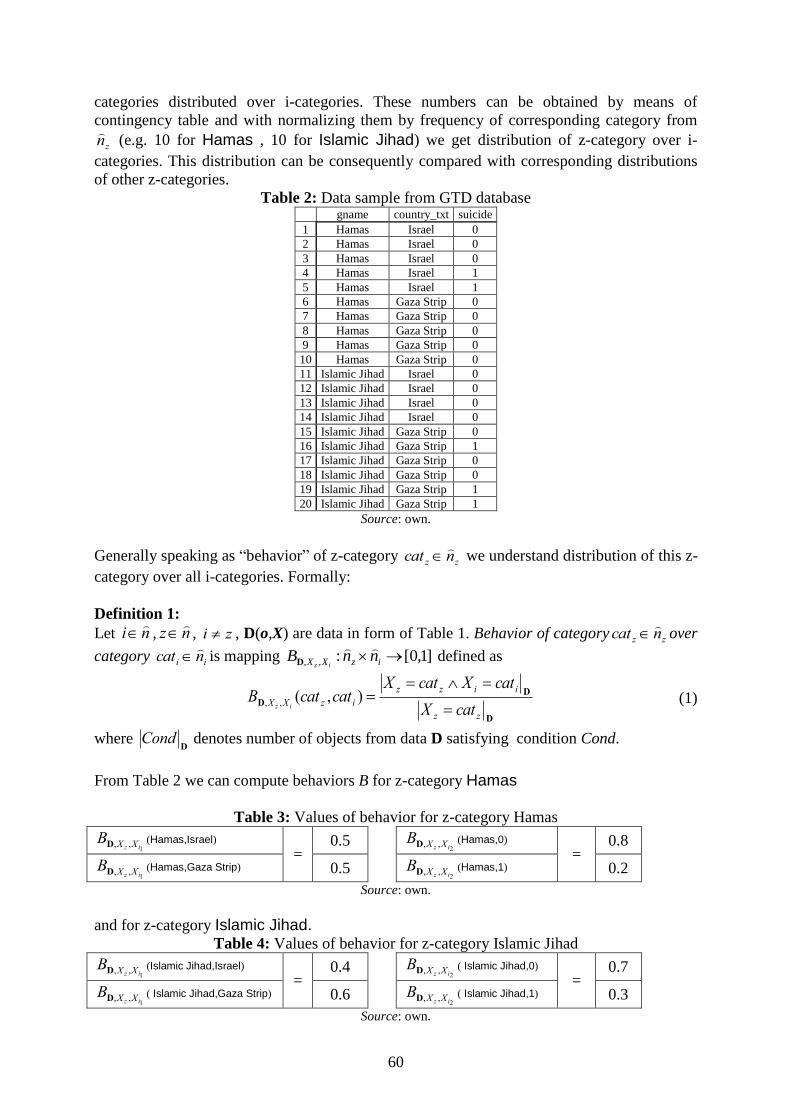
categories distributed over i-categories. These numbers can be obtained by means of

contingency table and with normalizing them by frequency of corresponding category from

zn

(e.g. 10 for Hamas , 10 for Islamic Jihad) we get distribution of z-category over i-

categories. This distribution can be consequently compared with corresponding distributions

of other z-categories.

Table 2: Data sample from GTD database gname country_txt suicide

1 Hamas Israel 0

2 Hamas Israel 0

3 Hamas Israel 0

4 Hamas Israel 1

5 Hamas Israel 1

6 Hamas Gaza Strip 0





11 Islamic Jihad Israel 0




15 Islamic Jihad Gaza Strip 0






Source: own.

Generally speaking as “behavior” of z-category zz ncat

we understand distribution of this z-

category over all i-categories. Formally:

Definition 1:

Let ni

, nz

, zi , D(o,X) are data in form of Table 1. Behavior of category zz ncat

over

category ii ncat

is mapping ]1,0[:,, izXX nnBiz

D

defined as

D

DD

zz

iizz

izXXcatX

catXcatXcatcatB

iz

),(,, (1)

where D

Cond denotes number of objects from data D satisfying condition Cond.

From Table 2 we can compute behaviors B for z-category Hamas

Table 3: Values of behavior for z-category Hamas

1,, iz XXBD (Hamas,Israel)

= 0.5

2,, iz XXBD (Hamas,0)

= 0.8

1,, iz XXBD (Hamas,Gaza Strip) 0.5

2,, iz XXBD (Hamas,1) 0.2

Source: own.

and for z-category Islamic Jihad. Table 4: Values of behavior for z-category Islamic Jihad

1,, iz XXBD (Islamic Jihad,Israel)

= 0.4

2,, iz XXBD ( Islamic Jihad,0)

= 0.7

1,, iz XXBD ( Islamic Jihad,Gaza Strip) 0.6

2,, iz XXBD ( Islamic Jihad,1) 0.3

Source: own.

61

After comparing these behavior values for each z-category (we compare differences between

values in pairs (1

,, iz XXBD (Hamas,Israel), 1

,, iz XXBD (Islamic Jihad,Israel)), (1

,, iz XXBD (Hamas, Gaza Strip),

1,, iz XXBD (Islamic Jihad, Gaza Strip)), (

2,, iz XXBD (Hamas, 0),

2,, iz XXBD (Islamic Jihad, 0)), etc., for all i-

categories) we can claim that behaviors of both z-categories are very similar (distributions of

objects belonging to each z-category over i-attributes are almost equal (i.e. not bigger than

0.1)). But this similarity is implied only when we compare z-categories over i-categories of

one other i-attribute at once (e.g. we first compare behavior values1

,, iz XXBD for Hamas with

corresponding values 1

,, iz XXBD for Islamic Jihad, then we compare behavior

values2

,, iz XXBD for Hamas with corresponding values 2

,, iz XXBD for Islamic Jihad and so on in

case there were more i-attributes). But if we investigate data deeper, we can observe that z-

categories doesn’t behave equal when both 1i

X and 2i

X are taken into account at one time.

For example, 2 attacks out of 5 taken by Hamas in Israel were committed by suicide

attacker, but for Islamic Jihad none of attacks in Israel was committed by suicide attacker.

So, distributions of z-categories over Cartesian product of i-categories are quite different and

to investigate these relations among categories of more than two attributes (i.e. among Xz and

more than one i-attribute) we formally define behavior of z-category zz ncat

over set of i-

categories kk iiii ncatncat ,...,

11as:

Definition 2:

Let i = {i1,...,ik}, n

i , nk

, nzz

i , D are data in form of Table 1. Behavior of

category zz ncat

over categories kk iiii ncatncat

,...,

11 is mapping

]1,0[...:11

,...,,, kkiiz iizXXX nnnB

D

defined as

D

DD

zz

iiiizz

iizXXXcatX

catXcatXcatXcatcatcatB

kk

kkiiz

...),...,,(

11

11,...,,, (2)

where D

Cond has the same meaning as in Definition 1.

With this definition we can compute behavior of z-categories over Cartesian product of i-

categories (21 ii nn

) which is now in form of matrix.

Source: own.

Source: own.

Table 5: Behavior values for Hamas on both i-categories

21,,, iiz XXXBD (Hamas,Israel,0)

21,,, iiz XXXBD (Hamas, Gaza Strip ,0)

= 0.3 0.5

21,,, iiz XXXBD (Hamas, Israel,1 )

21,,, iiz XXXBD (Hamas, Gaza Strip,1) 0.2 0

Table 6: Behavior values for Islamic Jihad on both i-categories

21,,, iiz XXXBD (Islamic Jihad,Israel,0)

21,,, iiz XXXBD (Islamic Jihad, Gaza Strip ,0)

= 0.4 0.3

21,,, iiz XXXBD (Islamic Jihad, Israel,1 )

21,,, iiz XXXBD (Islamic Jihad, Gaza Strip,1) 0 0.3

62

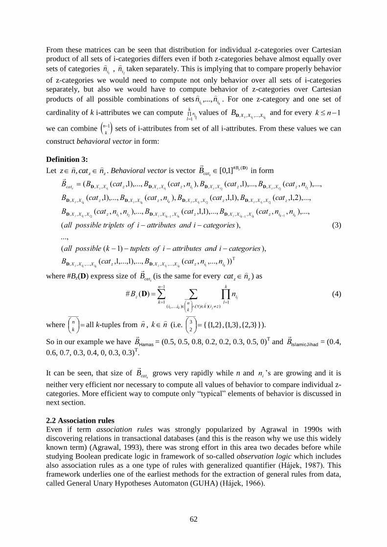
From these matrices can be seen that distribution for individual z-categories over Cartesian

product of all sets of i-categories differs even if both z-categories behave almost equally over

sets of categories 1i

n

, 2i

n

taken separately. This is implying that to compare properly behavior

of z-categories we would need to compute not only behavior over all sets of i-categories

separately, but also we would have to compute behavior of z-categories over Cartesian

products of all possible combinations of setskii nn

,...,

1. For one z-category and one set of

cardinality of k i-attributes we can compute

k

l li

n

1

values of kiiz XXXB ,...,,,

1D and for every 1 nk

we can combine k

n 1 sets of i-attributes from set of all i-attributes. From these values we can

construct behavioral vector in form:

Definition 3:

Let zz ncatnz

, . Behavioral vector is vector )(#

]1,0[Dz

z

B

catB

in form

T

,...,,,,...,,,

,,,,,,,,,

,,,,,,,,,,

,,,,,,,,

)),...,,(),...,1,...,1,(

),)1((

...,

),(

),...,,,(),...,1,1,(),...,,,(

),...,2,1,(),1,1,(),,(),...,1,(

),...,,(),...,1,(),,(),...,1,((

111

1112121

2121

222111

kkiizkiiz

kkkikizkikiziiz

iiziizkkizkiz

izizizizz

iizXXXzXXX

iizXXXzXXXiizXXX

zXXXzXXXizXXzXX

izXXzXXizXXzXXcat

nncatBcatB

categoriesiandattributesioftupletskpossibleall

categoriesiandattributesioftripletspossibleall

nncatBcatBnncatB

catBcatBncatBcatB

ncatBcatBncatBcatBB

DD

DDD

DDDD

DDDD

(3)

where #Bz(D) express size of zcatB

(is the same for every zz ncat

) as

1

1))((),...,(

11

)(#n

kzikj

k

nii

k

l

iz

jk

lnB

D (4)

where

k

nall k-tuples from n

, nk

(i.e. }}3,2{},3,1{},2,1{{

2

3

).

So in our example we have HamasB

= (0.5, 0.5, 0.8, 0.2, 0.2, 0.3, 0.5, 0)T and JihadIslamic B

= (0.4,

0.6, 0.7, 0.3, 0.4, 0, 0.3, 0.3)T.

It can be seen, that size of zcatB

grows very rapidly while n and in ’s are growing and it is

neither very efficient nor necessary to compute all values of behavior to compare individual z-

categories. More efficient way to compute only “typical” elements of behavior is discussed in

next section.

2.2 Association rules

Even if term association rules was strongly popularized by Agrawal in 1990s with

discovering relations in transactional databases (and this is the reason why we use this widely

known term) (Agrawal, 1993), there was strong effort in this area two decades before while

studying Boolean predicate logic in framework of so-called observation logic which includes

also association rules as a one type of rules with generalized quantifier (Hájek, 1987). This

framework underlies one of the earliest methods for the extraction of general rules from data,

called General Unary Hypotheses Automaton (GUHA) (Hájek, 1966).

63

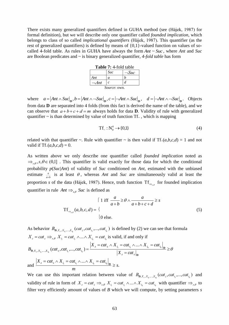
There exists many generalized quantifiers defined in GUHA method (see (Hájek, 1987) for

formal definition), but we will describe only one quantifier called founded implication, which

belongs to class of so called implicational quantifiers (Hájek, 1987). This quantifier (as the

rest of generalized quantifiers) is defined by means of {0,1}-valued function on values of so-

called 4-fold table. As rules in GUHA have always the form SucAnt ~ , where Ant and Suc

are Boolean predicates and ~ is binary generalized quantifier, 4-fold table has form

Table 7: 4-fold table Suc Suc

Ant a b

Ant c d

Source: own.

where D

SucAnta ,D

SucAntb ,D

SucAntc , D

SucAntd . Objects

from data D are separated into 4 folds (from this fact is derived the name of the table), and we

can observe that mdcba always holds for data D. Validity of rule with generalized

quantifier ~ is than determined by value of truth function Tf~ , which is mapping

}1,0{N:Tf 4

0~ (4)

related with that quantifier ~. Rule with quantifier ~ is then valid if Tf~(a,b,c,d) = 1 and not

valid if Tf~(a,b,c,d) = 0.

As written above we only describe one quantifier called founded implication noted as

]1,0(,,, ss . This quantifier is valid exactly for those data for which the conditional

probability p(Suc|Ant) of validity of Suc conditioned on Ant, estimated with the unbiased

estimate ba

a

is at least , whereas Ant and Suc are simultaneously valid at least the

proportion s of the data (Hájek, 1987). Hence, truth function ,

Tfs for founded implication

quantifier in rule SucAnt s , is defined as

1 iff sdcba

a

ba

a

),,,(Tf,

dcbas

(5)

0 else.

As behavior ),...,,(11

,...,,, kkiiz iizXXX catcatcatBD is defined by (2) we can see that formula

kkll iiiiszz catXcatXcatX ..., is valid, if and only if

D

DD

zz

iiiizz

iizXXXcatX

catXcatXcatXcatcatcatB

kk

kkiiz

...),...,,(

11

11,...,,,

and ....

11

sm

catXcatXcatXkk iiiizz

D

We can use this important relation between value of ),...,,(11

,...,,, kkiiz iizXXX catcatcatBD and

validity of rule in form of kkll iiiiszz catXcatXcatX ..., with quantifier ,s to

filter very efficiently amount of values of B which we will compute, by setting parameters s

64

and θ, and also we solve the problem of extremely large amount of values determined by

)(# DzB .

As we see from definition of behavioral vector (3), there is just one corresponding formula for

each element j of zcatB

for k-tuples of i-attributes

kii XX ,...,1

and i-categories

kiiz catcatcat ,...,,1

, so we denote it as

jcatzBformula )((

) = (kkll iiiiszz catXcatXcatX ..., ). (6)

Together with this we denote

))((Tf

, jcatzsB

= ),,,(Tf,

dcbas (7)

for formula jcatzBformula )((

). We construct set of indexes J

))((()(|{ jcatzz z

BformulancatjJ

N is valid for data D) } (8)

and then we can construct vector of reduced size, which we call typical behavior vector

denoted as zcatTypical B

and which is constructed only from selected (by set of indexes J) values

of zcatB

as:

Definition 4:

Let zz ncatnz

, , ]1,0(, s , zcatB

is behavioral vector (from Def. 3) and symbols J and

))((Tf, jcatzsB

have meaning from (8) and (7), respectively. Then typical behavior vector for

zcat (noted zcatTypical B

) is defined as

JlBBB jcatJcatlcatTypical zslzz

#,...,1),)((Tf)()(,

, (9)

where #J denotes cardinality of set J. Vector zcatTypical B

is of course s and θ dependent, but to

not overcomplicate notation we omit it.

So general process of construction of zcatTypical B

consists of three steps:

1. extraction of all valid rules in form kkll iiiiszz catXcatXcatX ..., and to

each rule compute corresponding behavior value ),...,,(11

,...,,, kkiiz iizXXX catcatcatBD ,

2. construction of set of indexes J (8),

3. construction of zcatTypical B

according to Definition 4.

To clarify more the process of construction of typical behavior vector, let’s look on our

example. First step is to set values of s and θ. By setting those two parameters we define the

meaning of term “typical” behavior. By setting parameter s closer to 1 we filter low

frequented combinations of all categories (z-category and i-categories) and with setting

parameter θ closer to 1 we filter low values of behavior B, focusing rather on values

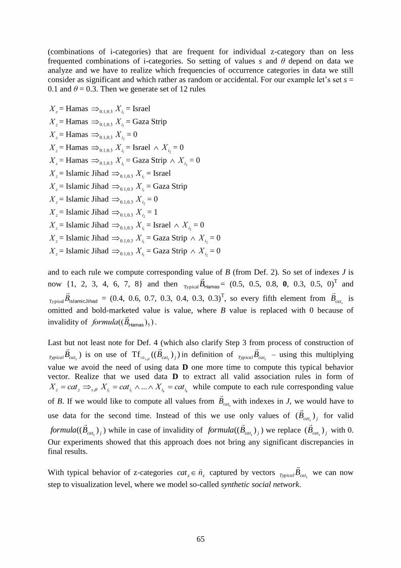
65

(combinations of i-categories) that are frequent for individual z-category than on less

frequented combinations of i-categories. So setting of values s and θ depend on data we

analyze and we have to realize which frequencies of occurrence categories in data we still

consider as significant and which rather as random or accidental. For our example let’s set s =

0.1 and θ = 0.3. Then we generate set of 12 rules

zX = Hamas 3.0,1.0li

X = Israel

zX = Hamas 3.0,1.0li

X = Gaza Strip

zX = Hamas 3.0,1.02i

X = 0


X = Israel 2i

X = 0


X = Gaza Strip 2i

X = 0

zX = Islamic Jihad 3.0,1.0li

X = Israel

zX = Islamic Jihad 3.0,1.0li

X = Gaza Strip

zX = Islamic Jihad 3.0,1.02i

X = 0


X = 1


X = Israel 2i

X = 0


X = Gaza Strip 2i

X = 0


X = Gaza Strip 2i

X = 0

and to each rule we compute corresponding value of B (from Def. 2). So set of indexes J is

now {1, 2, 3, 4, 6, 7, 8} and then HamasB

Typical = (0.5, 0.5, 0.8, 0, 0.3, 0.5, 0)T and

JihadIslamic B

Typical = (0.4, 0.6, 0.7, 0.3, 0.4, 0.3, 0.3)T, so every fifth element from

zcatB

is

omitted and bold-marketed value is value, where B value is replaced with 0 because of

invalidity of ))(( 5HamasBformula

.

Last but not least note for Def. 4 (which also clarify Step 3 from process of construction of

zcatTypical B

) is on use of ))((Tf, jcatzs

B

in definition of zcatTypical B

– using this multiplying

value we avoid the need of using data D one more time to compute this typical behavior

vector. Realize that we used data D to extract all valid association rules in form of

kkll iiiiszz catXcatXcatX ..., while compute to each rule corresponding value

of B. If we would like to compute all values from zcatB

with indexes in J, we would have to

use data for the second time. Instead of this we use only values of jcatzB )(

for valid

jcatzBformula )((

) while in case of invalidity of jcatzBformula )((

) we replace jcatzB )(

with 0.

Our experiments showed that this approach does not bring any significant discrepancies in

final results.

With typical behavior of z-categories zz ncat

captured by vectors zcatTypical B

we can now

step to visualization level, where we model so-called synthetic social network.

66

3 Social network model

A social network (SN) is typically a set of people or groups of people with similar pattern of

contacts or interactions such as friendship, co-working, or information exchange (Wasserman,

1994). Social networks are usually represented using graph theory (with graphs), where nodes

represent individuals or groups and lines represent relations among them (Carrington, 2005).

These graphs can be directed or undirected, depending on the type of the relation between the

linked nodes. To designate different interaction strengths, there can be assigned weights to the

links (edges) between the nodes. Using other additional information (often not directly related

to the interactions, e.g. behavior), we can construct synthetic social networks, where the

relations between the nodes can be represented by the similarity of this kind of information

(e.g. similar typical behavior).

3.1 Computing similarities and visualization of social network model

From the previous data mining level related to the extraction of the association rules, we have

constructed set of vectors zcatTypicalB

for every z-category zz ncat

(Def. 4). Consequently

from this set of nz behavioral vectors we have created Similarity matrix zz nnS

[0,1] using

Cosine measure for computing the similarity jis , between two objects io zn

and jo zn

(terrorist groups)(Han, 2006):

J

k

kjTypical

J

k

kiTypical

J

k

kjTypicalkiTypical

ji

BB

BB

s#

1

2#

1

2

#

1,

)()(

)()(

(10)

for zz njni

, .

Source: own.

Model of the synthetic social network was obtained using principles of graph theory. The

model was constructed with the undirected weighted graph G = (O, E) where O is set of

Figure 3: Synthetic Social Network based on 12 i-attributes

67

objects (terrorist groups) from the Similarity matrix and E is set of edges, which represent

relations between them. The weight of the edges is defined using the similarity measure jis , .

4 Experiments

The initial graph contained 33 nodes with 528 edges (which represents one large connected

component). For discovering significant communities with similar behavior we processed the

edge filtering and graph partitioning based on the selected level of edge weight > 0.6. For the

visualization of the SN model was used the algorithm Force Atlas. The visualization was

provided for both experiments with different number of selected attributes characterizing the

similar behavior of the terrorist groups (see section 2.2). In the Table 7 there are presented

parameters of both obtained graphs after the filtering and the graph partitioning.

Table 8: Graph Parameters Experiment 1 Experiment 2

i-Attributes 8 12

Extracted rules 2005 9252

Nodes before filtering 33 33

Edges before filtering 528 528

Nodes after filtering 12 (36,36%) 17 (51,52%)

Edges after filtering 66 (12,5%) 136 (26,73%)

Number of communities 5 4

Modularity 0.6875 0.594

Source: own.

On the figures 2 and 3 we can see the visual representation of the models of synthetic social

networks constructed from the GDT database for the year 2001 using the open-source

software Gephi. The first graph (Figure 2) was obtained for the 8 selected i-attributes, the

second (Figure 3) for 12 i-attributes. Both graphs show communities of terrorist groups with

similar behavior. The width of the edges represents the strength of the relation (based on

value of similarity) between terrorist groups. From both graph we can see, that the community

detection can be influenced by the selection of appropriate attributes (which can depend on

the user requirements).

Conclusion

The paper is oriented to the modeling of the synthetic social network based on the similar

behavior of the terrorist groups extracted from the data collection GDT. The expression of

typical behavior was formalized using the association rules mining method; the similarity

between the terrorist groups based on their typical behavior was then analyzed and visualized

using the methods of the graph theory. As an example there were processed two experiments

with the different amount of selected attributes and two models of the synthetic social

network were presented. The obtained graphs showed that the proposed data mining method

is effective and can facilitate the orientation in the large amount of the extracted association

rules. The extracted information can be applied in the prediction process or for construction of

classification models using the relations within the data records or between the data

collections. This type of information can be valuable in the decision making process and

forecast the effects of those decisions. The proposed model then can be helpful in the

identification process of the attacker or known terrorist group in the situations, when incident

occurs. Also, it must be noted that the proposed approach involves rich parametric

configuration and thus, for a practical use, there will be required the knowledge of domain

experts. In future work we intent to visualize the evolution of the obtained synthetic social

network model.

68

References

[1] AGRAWAL, R., T. IMIELINSKI and A. SWAMI, 1993. Mining association rules

between sets of items in large databases. In Proc. 1993 ACM-SIGMOD Int. Conf.

Management of Data (SIGMOD’93), Washington, DC, pp. 207–216.

[2] BENOÎT, G., 2002. Data Mining. Annual Review of Information Science and

Technology. Vol. 36, pp 265-310.

[3] CARRINGTON P. J., J. SCOTT and S. WASSERMAN, 2005. Models and Methods

in Social Network Analysis. Cambridge: Cambridge University Press.

[4] FREEMAN, L. C., 2004. The Development of Social Network Analysis: A Study in the

Sociology of Science. Empirical Press.

[5] GODWIN, A., R. CHANG, R. KOSARA and W. RIBARSKY, 2008. Visual analysis

of entity relationships in global terrorism database. In SPIE Defense and Security

Symposium.

[6] HÁJEK, P. and T. HAVRÁNEK, 1987. Mechanizing Hypothesis Formation. Springer

Verlag, Berlin.

[7] HAN, J. and M. KAMBER, 2006. Data Mining Concepts and Techniques. Elsevier

Science Ltd., pp 745. ISBN 1-55860-901-6.

[8] HAND, D. J., P. SMYTH and H. MANILLA. Principles of Data Mining. MIT Press,

2001. ISSN 0-262-08290-X.

[9] LAFREE, G. and L. DUGAN, 2007. “Global Terrorism Database 1970-1997”,

[Computer file]. ICPSR04586-v1. College Park, MD: University of Maryland

[producer], 2006. Ann Arbor, MI: Inter-university Consortium for Political and Social

Research [distributor].

[10] LEE, J., 2008. Exploring Global Terrorism Data: A Web-based Visualization of

Temporal Data. In ACM Crossroads, Vol. 15, (2), pp. 7-16.

[11] ŠIMŮNEK, M., 2003. Academic KDD project LISP-Miner. In A. Abraham, K.

Franke, K. Koppen (Eds.), Advances in Soft Computing – Systems Design and

Applications. Springer Verlag, Heidelberg, pp. 263–272.

[12] WASSERMAN, S. and K. FAUST, 1994. Social Network Analysis. Cambridge:

Cambridge University Press.

[13] P. HAJEK, I. HAVEL and M. CHYTIL, 1996: The GUHA method of automatic

hypotheses determination. Computing 1, fasc. 4, 293—308.

[14] JONES, J., R. CHANG, T. BUTKIEWICZ and W. RIBARSKY, 2008. Visualizing

uncertainty for geographical information in Global Terrorism Database. In SPIE

Defense and Security Symposium.

[15] KOSARA, R., F. BENDIX and H. HAUSER, 2006. Parallel sets: visual analysis of

categorical data. IEEE Transactions on Visualization and Computer Graphics

12(4):558-564.

[16] WANG, X., E. MILLER, K. SMARICK, W. RIBARSKY and R. CHANG, 2008.

Investigative visual analysis of Global Terrorism Database. In Journal of Computer

Graphics Forum. Volume 27, Issue 3, pages 919–926, May 2008.

[17] ZHANG, H., B. CLARK and E. FOKOUÉ, 2009. Principles and theory for Data

Mining and Machine Learning. Springer.

Documents

BUILDING SYNTHETIC SOCIAL NETWORKS USING ASSOCIATION …