Embed Size (px)
Citation preview

Munich Personal RePEc Archive
Bubble Bank
Osadchiy, Maksim and Sidorov, Alexander
Corporate Finance Bank (Russia, Moscow), Novosibirsk StateUniversity and Sobolev Institute of Mathematics (Russia,Novosibirsk)
22 July 2019
Online at https://mpra.ub.uni-muenchen.de/95995/
MPRA Paper No. 95995, posted 14 Sep 2019 16:05 UTC
Bubble Bank∗
Maksim Osadchiy†, Alexander Sidorov‡
September 12, 2019
Abstract
The paper considers a bank, left to itself, outside of regulation and supervision. The stochastic
model allows us to describe the parameters, which create conditions both for the formation of
bubbles in the credit market and for the formation of stable banks with self-restrictive behavior that
do not require regulatory intervention. The comparative statics of equilibria is studied with respect
to the basic parameters of the model, a theoretical assessment is carried out of the probability
of bank default based on the values of exogenous factors. Our main task is to evaluate a bank
probability of default not by using an econometric empirical approach, but by using microeconomic
modeling.
Key words: Banking microeconomics, Credit bubble, Probability of default, Capital adequacy ratio
JEL codes: G21, G28, G32, G33
Introduction
The aim of the work is to study credit bubbles and ability of banks to self-restraint - refusal from
unlimited credit expansion without regulatory intervention. The applied task of the study is to create a
method for calculating bank ratings based on microeconomic analysis, and not on empirical econometric
models. Of course, one cannot finally get rid of empiricism in calculating bank ratings, since many
risk factors of bank default cannot be calculated using only microeconomic models, for example, the
quality of management and internal control, reputation, etc.
The motivation of the paper is the inclusion in the microeconomic model of the bank of a relatively
realistic Vasicek portfolio loss density function, taking into account the correlation of the assets of
∗We thank Henry Penikas for the useful comments and suggestions, and Dirk Tasche for the kind assistance injustification of Example. Authors are thankful to participants of the seminar in Sobolev Institute of Mathematics foruseful discussion. This study has been funded by Russian Foundation for Basic Research, Project No. 18-010-00728.
†Corporate Finance Bank (Russia, Moscow). Email: [email protected]‡Novosibirsk State University and Sobolev Institute of Mathematics, Siberian Branch of the Russian Academy of
Sciences (Russia, Novosibirsk) Email: [email protected]
1

borrowers to assess the risk of default of the bank, as well as to study the structure of assets and
liabilities of the bank. However, in this paper we will consider the more general form of the portfolio
loss density function, not limited to the Vasicek model.
Our work is based on 4 stylized facts related to the field of credit risks:
(1) Many banks tend to blow bubbles - to carry out dangerous credit expansion. They turn into
“black holes” - fast-growing banks with unobservable negative capital. This problem is especially acute
in developing countries with poor quality of banking regulation and supervision.
(2) If credit expansion covers the entire banking sector, a credit boom begins. If it is not stopped
in time, it will inevitably end in a credit crisis. History knows hundreds of examples of such crises (see,
e.g., [17, pp. 344-347]). For example, the burst of the US subprime mortgage bubble caused a global
crisis.
(3) Credit crises lead to high social costs - unemployment, impoverishment, social instability. To
avoid such severe consequences, the regulators limit the expansion of banks by micro-prudential policies,
in particular, limiting by CAR (capital adequacy ratio) from below.
(4) Instead of maximally using a capital and increasing risk assets up to the level close to the
capital adequacy requirements imposed by the regulator, many banks far exceed the CAR regulatory
requirements. CAR has a wide spread [4, Graph I.13]: many banks are undercapitalized, and many
banks are overcapitalized.
The key question of the paper: is the bank capable of self-restraint, under certain conditions,
without the intervention of the regulator? We will also consider the question: why there is such a large
spread of CAR and what explains its magnitude? To do this, consider a hypothetical bank operating
without external regulation, and study its behavior. We will build a simple microeconomic model of
the bank that takes into account only credit risk.
Our belongs to the class of the Structural models of credit risk. In the framework of our paper a
bank is considered as a “Merton firm” with the balance including, on the one hand, the stochastically
changing portfolio of assets, on the other hand, the given (i.e., risk-free) liabilities and capital. In
turn, the behavior of the assets portfolio is captured by the Vasicek model [19, 20], i.e., as an infinite
number of liabilities of the Merton-type firms with the correlating firm’s assets. The main result of the
Vasicek approach is a derivation of the portfolio’s probability density function (PDF) of credit losses,
also known as loss distribution of a credit portfolio, from the Brownian motion of the firm’s assets.
The Vasicek’s portfolio credit loss model [19] underlies the Basel Advanced Internal Rating System
(AIRB), which was developed to determine regulatory requirements for bank capital, well-known as
Basel II and Basel III [3]. Although in reality the credit risk is often accompanied by the risk of outflow
2
of liabilities, in the framework of this paper we do not allow for the liquidity risk, leaving it for a future
research.
Similarly to the Merton model, our approach allows to assess the probability of the bank default,
which take place when the assets portfolio falls lower than liabilities. However, the main difference
of our approach from the Merton model is that we account for the bankruptcy charges. Moreover,
the result of our paper shows that this factor plays the crucial role in the banker’s decision making.
Within the framework of the model, we construct the parameter zones where the bank is capable
of self-restraint and where the bubble inflates - unlimited expansion takes place. We will study the
structure of these areas. We will also calculate the probability of default of the bank and determine
the structure of assets and liabilities of the bank within our model. And we will study the dependence
of the probability of default of the bank and its CAR on the parameters.
Using the model, we study the mechanism of CAR choice. We study also the comparative statics of
the banker’s decision and of the probability of the bank’s default with respect to the model parameters:
the interest rates of attraction and allocation of resources, the correlation of borrowers’ assets and other
factors. There are identified the three areas in the space of exogenous parameters within which the
banks are capable of self-restraint, and when they choose the unlimited expansion. This zoning of the
model parameters, according to the nature of the equilibrium solution, opens a new way to determine
whether the regulator is needed to intervene in banking, what are the boundaries of this intervention
and its effectiveness. On the one hand, the concept of laissez-faire can be destructive, since the banking
market failure entails far-reaching negative consequences, not so much even for the bank owner as for
its many clients. If the bank is large enough, then its default can cause a domino effect. On the other
hand, practice shows that the tightening of regulation is faced with the problem of low efficiency of
regulatory measures, since banks have ample opportunities to manipulate information, creating the
appearance of compliance with regulatory constraints. Another negative effect of over-regulation is a
decrease in the efficiency of banks and the economy as a whole. As regulation is tightened, bankers
spend too much time and efforts on compliance, instead of doing business. In this regard, it is worth to
recall the general economic principle, according to which an economic individual can bypass external
constraints, but cannot ignore his/her own incentives.
The classification of the solutions obtained in this paper allows us to identify cases when a state
intervention in the bank activity is superfluous, since the decision satisfying the regulator is supported
by internal stimuli. If the decision falls into another class, for example, it is characterized by an
excessively low CAR, then this intervention is inevitable. Rating agencies use to apply the empirical
econometric models to calculate the credit ratings. Our model allows to consider the prospect of
3

calculating bank credit ratings not with empirical econometric models, but with micro-based modeling.
Microeconomic models can be useful for evaluating implications of banking regulation.
The paper is organized as follows. Section 1 presents the model of bank that takes into account the
partial impairment of bank assets in the event of a bank default, and the conditions for the existence
and uniqueness of the equilibria are obtained. The mechanism of the formation of an equilibrium
market credit rate in a competitive environment of risk-neutral players is considered. In Section 2,
we consider the parametrized classification of the equilibrium states based on CAR and study the
comparative statics of equilibrium characteristics both analytically and using computer simulation.
Section 3 is devoted to a more visual graphical classification of decisions on the main parameters. The
most important result is the determination of compliance with the requirements of Basel III. Finally,
Section 4 is devoted to the multi-period extension of this model, in particular, the assessment of the
probability of a bank’s default in the long term is found. The main results and conclusions of the work
are formulated in the Conclusion. A list of notations and abbreviations is placed at the beginning of
Appendix.
The related literature
There are two primary types of models that attempt to describe default processes in the credit risk
literature: structural and reduced form models. The aim of structural approach is to provide a rela-
tionship between default risk and capital structure, unlike the reduced form models, which consider
the credit default as exogenous event driven by a stochastic process. Reduced form models do not
consider the relation between default and firm value in an explicit manner. Intensity models represent
the most extended type of reduced form models. In contrast to structural models, the time of default
in intensity models is not determined via the value of the firm, but it is the first jump of an exogenously
given jump process. The parameters governing the default hazard rate are inferred from market data.
Structural models, pioneered by Black, Scholes [6]and Merton [15], ingeniously employ modern option
pricing theory in corporate debt valuation. Merton model was the first structural model and has served
as the cornerstone for all other structural models, including ours. A significant extension of Merton
was represented by Black and Cox in [5], who managed to relax some of the Merton’s assumption.
The next major step in generalizing the structural models was an important contribution of Leland
in [13], who explicitly introduced corporate taxes and bankruptcy costs, which may be interpreted as
liquidation costs. Thus, he formalized the trade-off framework and provided a way to determine both
the optimal default boundary and the value-maximizing optimal capital structure. Since these classical
papers the further advances of structural models in various direction. It worth to mention that firms
4
often make their decisions in a principal agent setting, wherein managers, equity holders (borrowers),
and creditors may have very different objective functions. The resulting agency problems may have
significant implications for the optimal capital structure decisions and optimal contracting decisions,
see the papers [9, 10]. The paper [1] develops a structural model of a financial institution that can
invest in both liquid and illiquid assets dynamically, maximizing the profit of its shareholders while
satisfying some regulatory constraints. It is proved that tightening the liquidity constraint adversely
affects their rates of return, while preventing some large losses that occur when the portfolio is very
illiquid.
The academic literature on jointly optimal regulation of bank capital and liquidity seems to increase
after 2010 by the Basel Committee on Banking Supervision. The paper [2] analyses how banking firms
set their capital ratios, that is, the rate of equity capital over assets. In order to study this issue,
two theoretical models are developed: the “market” model for banks not affected by capital adequacy
regulation, while the second one, the regulatory model, explain the behavior of banks with an optimal
market ratio below a legally required regulation.
Regulation related to capital requirements is an important issue in the banking sector. One of the
indices used to measure how susceptible a bank is to failure, is the capital adequacy ratio (CAR). In
general, this index is calculated by dividing a measure of bank capital by an indicator of the level
of bank risk. The papers [11] and [16] consider the application of stochastic optimization theory to
asset and capital adequacy management in banking and construct continuous-time stochastic models
for the dynamics of capital adequacy ratio established by Basel II. This ratio is obtained by dividing
the bank’s eligible regulatory capital (ERC) by its risk-weighted assets (RWAs) from credit, market
and operational risk. The contribution of paper [7] is the construction of a stochastic dynamic model
to describe the evolution of bank capital that incorporates capital gains and losses. The gains and
losses are represented by loan loss reserves and the unexpected loan losses, respectively. It is studied
the optimal capital management problem which maximizes the expectation of bank capital under a
risk constraint on the Capital-at-Risk (CaR), where CaR is defined in terms of Value-at-Risk (VaR).
The issue of bank capital adequacy and risk management within a stochastic dynamic setting is
studied in the paper [8]. An explicit risk aggregation and capital expression is provided regarding the
portfolio choice and capital requirements special context. This leads to a nonlinear stochastic optimal
control problem whose solution may be determined by means of dynamic programming algorithm.
Along with the great impact of structural models on the theory of the credit risk and its application,
there is reasonable criticism on the prediction power of such models concerning to the pricing of
corporative bonds, see, for example, [12]. On the other hand, the structural models are able to predict
5

well the hedge ratios of corporate bonds against the equity of the underlying firm, see [18]. Concluding
this short survey of structural models one can say: “All models are wrong, but some are useful.”
1 The model
We follow Vasicek approach [20], assuming that the bank provided n loans, and the probability of
default of each loan i ∈ {1, . . . , n} is the same and equals to PD ∈ [0, 1]. It is assumed that the loss
given default LGD = 1. Random variable εi takes two possible values: εi = 1, if credit i is defaulted
(with probability PD), and εi = 0 (with probability 1 − PD) otherwise. Generally speaking, the
random variables εi, i ∈ {1, . . . , n} are not independent. Then a random variable
ε = limn→∞
1
n
n∑
i=1
εi
characterizes the share of nonperforming loans, taking values in the interval [0, 1]. It is obvious that
E(ε) = PD, while the distribution of ε is not necessary normal due to possible dependence of various
εi. For now we don’t take any specific assumptions on the nature of this dependence, considering
the general Cumulative Distribution Function (CDF) F (z) of the random variable ε on [0, 1]. Further
we put some natural assumption on F (z), which encompass the most important case of the Vasicek
distribution of losses.
It is assumed that the bank operates in a perfectly competitive environment, being a price taker.
We study a single-period model in which a bank is created at the initial moment t = 0 with an initial
capital K0 > 0. At the same time the banker chooses the amount D0 ≥ 0 of the attracted deposits
at the interest rate R > 0, and then places the borrowed and its own funds in the uniform loans of
the same size at the interest rate r > R before the terminal moment t = 1, hence, the loans are equal
to L0 = K0 +D0. The supply of loans and the demand for deposits are satisfied in full, and interest
rates are exogenous parameters, due to the assumption of perfectly competitive environment. At the
moment t = 1 all loans are repaid, except for those defaulted, hence L1 = 0, and all assets acquire the
form of cash M1. After the deposits are returned and interest is paid at the rate R, the bank’s capital
becomes equal to K1 = M1 −D1.
All balance sheet items, are summarized in Table 1.
Remark 1. This model can be extended to the case of the arbitrary cash M0 ≥ 0. However, given
the lack of liquidity risk, i.e., the nonzero probability of the premature withdrawal of deposits, easily
implies that the optimum choice of the banker will be M0 = 0.
Suppose that the bank’s default implies the additional losses, moreover, the banker is “responsible”
6

Balance sheet items t = 0 t = 1
AssetsCash M0 = 0 M1 = (1 + r)L0(1− ε)Loans L0 = K0 +D0 L1 = 0
Deposits D0 ≥ 0 D1 = (1 +R)D0
Capital K0 > 0 K1 = M1 −D1
Table 1: Control variables and dependencies between variables
i.e., bears all the costs of bankruptcy. More precisely, if random amount of bank capital at the end of
the period
K1 = (1 + r)L0(1− ε)− (1 +R)D0
takes positive value, then this amount goes to the banker unchanged. Given D0 = L0−K0, this means
that
K1 = (r −R− ε(1 + r))L0 + (1 +R)K0.
Otherwise, in case of default i.e., K1 ≤ 0, the bank sells a loan portfolio with a discount 0 ≤ d ≤ 1.
As result, the terminal capital under default is equal to
K1 = K1 − d(1 + r)L0(1− ε).
The value d = 0 corresponds to the case when there are no additional losses, i.e., K1 = K1.
Note that the condition of the bank default
K1 ≤ 0 ⇐⇒ ε ≥ r −R
1 + r+
1 +R
1 + r
K0
L0. (1.1)
In other words, the default takes place if and only if the losses exceed the certain threshold, which
depends on the Capital Adequacy Ratio (CAR)
k(L0) =K0
L0.
Here we assume that the risk weight of loans is equal to 1.
To save space, let’s introduce the following notification
E =r −R
1 + r,
which implies
1 +R
1 + r= 1− E , r −R
1 + r= E − PD,
7
and let
E(k) = E + (1− E)k.
Due to (1.1) E(k(L0)) may be interpreted as a threshold value of losses, which triggers the bank default.
The value E = E(0) may be also interpreted as the limit loss threshold when the loan portfolio increases
unrestrictedly, because limL0→∞
k(L0) = 0.
Thus, the general definition of the terminal capital is
K1 =
K1, if ε < E(k(L0))
K1 − d(1 + r)L0(1− ε), otherwise.
The banker’s problem is to maximize the expected value of the terminal capital E(K1) under condition
D0 ≥ 0 ⇐⇒ L0 ≥ K0. Given
E(K1) = (r −R− PD(1 + r))L0 + (1 +R)K0 = (1 + r)[
(E − PD)L0 + (1− E)K0
]
,
we obtain that the expected terminal capital is equal to
E(K1) = (1 + r)
[
(E − PD)L0 + (1− E)K0 − dL0
∫ 1
E(k(L0))(1− z)f(z)dz
]
.
Given f(z) = F ′(z) is a PDF of the random losses ε, we may interpret the function
ret(z) ≡ (1− z)f(z)
as a weighted share of the returned loans and let
Ret(x) =
∫ 1
x
ret(z)dz.
The function Ret(x) is obviously decreasing, because Ret′(x) = −ret(x), and satisfies Ret(0) = 1−PD,
Ret(1) = 0. Therefore, the expected terminal capital E(K1) = (1 + r)U(L0), where
U(L0) = (1− E)K0 + (E − PD)L0 − d · L0Ret(E(k(L0))), (1.2)
is the reduced objective function.
8

Now the original banker’s problem is equivalent to
maxU(L0) s.t. L0 ≥ K0.
Theorem 1. Let r > R and the weighted share of returns ret(z) is strictly decreasing on the interval
PD < z < 1, then U ′′(L0) < 0 for all L0 ≥ K0. Moreover, if inequality
d >E − PD
Ret(E)(1.3)
holds, then there exists unique solution of the banker’s problem
L∗0 =
K0
k∗, D∗
0 =1− k∗
k∗K0 (1.4)
where k∗ ∈ (0, 1) is an equilibrium CAR, defined as the unique solution of equation
FOC : E − PD − d ·(
Ret(E(k)) + (1− E)k · ret(E(k)))
= 0. (1.5)
Proof. See Appendix A.1.
Theorem 1 implies that depending on the parameter’s relation, there may be two possible cases,
which cause different types of the banker’s behavior.
Case 1. Let the discount d be sufficiently small, e.g., d = 0, so that condition (1.3) is violated.
This implies an unrestricted increasing of objective function U(L0) when L0 → +∞, which means that
banker has incentives for unrestricted expansion1 of the loan portfolio L0.
To prevent this negative trend, the regulator restricts lending by imposing the condition
K0/L0 ≥ k ⇐⇒ L0 ≤ L0(k) =K0
k. (1.6)
for the exogenously given CAR k. It is obvious that in this case, the modified banker problem with
additional constraint (1.6) has solution L∗0 = L0(k).
Case 2. Assume that the discount d is sufficiently large to satisfy the condition (1.3) and, therefore,
there exists solution k∗ ∈ (0, 1) of (1.5). This situation can be interpreted as if the banker imposes
self-restrain L0 ≤ K0/k∗, which is active in the optimum, i.e., L∗
0 = K0/k∗ > K0.
Remark 2. The first order condition (1.5) may be interpreted in terms of the gains-losses as follows.
Choosing the amount of the loans portfolio L0 the banker obtains the expected total gains (1−E)K0+
1The same holds when banker is “irresponsible”, i.e., does not want to pay his/her liabilities in case of default, i.e.,K1 = 0.
9
(E − PD)L0, thus the marginal gains from the further credit expansion are
E − PD =r −R
1 + r.
On the other hand, the term
Ret(E(k(L0))) =
∫ 1
E(k(L0))ret(z)dz = E(1− ε| ε > E(k(L0)))
characterizes the share of the the loans returns in case of the bank default. Note that the size of the
loan portfolio affects both the basis L0 and the share of returns E(1− ε| ε > E(k(L0))), then the total
marginal losses in case of the bank default are sum of effects: the marginal losses from increasing of
basis L0 are equal to
d · Ret(E(k(L0))),
while the losses from change of share are equal to
d · L0
(
−ret(E(k(L0)))d
dL0E(k(L0))
)
= d · (1− E)k(L0)ret(E(k(L0))).
Finally, the gross marginal losses are equal to
d ·(
Ret(E(k(L0))) + (1− E)k(L0)ret(E(k(L0))))
,
Thus, the FOC 1.5 is equivalent to coincidence of the marginal gains and the marginal losses.
The Vasicek distribution of losses
To justify the conditions of Theorem 1, consider the Vasicek distribution of the loan losses (see [20])
with CDF
F (z;PD, ρ) = Φ
(√1− ρΦ−1(z)− Φ−1(PD)√
ρ
)
, (1.7)
where PD is a probability of a borrower’s default, ρ is a correlation coefficient of a borrower’s assets.
The corresponding PDF is as follows
f(z;PD, ρ) =
√
1− ρ
ρexp
(
1
2
[
(Φ−1(z))2 −(√
1− ρΦ−1(z)− Φ−1(PD)√ρ
)2])
. (1.8)
Lemma 1. Let 0 < ρ < 1, 0 < PD < 1 and f(z;PD, ρ) be the density function of the Vasicek
distribution of losses. Then the function ret(z;PD, ρ) ≡ (1− z)f(z;PD, ρ) decreases with respect to z
10

in interval PD < z < 1.
Proof. See Appendix A.22.
1.1 Comparative statics of equilibrium
Now we will study how the equilibrium reacts to the changes of the parameters d, R and r.
Proposition 1. The signs of partial derivatives of the equilibrium values of k∗, L∗0, D
∗0 with respect to
d, R, and r are as follows:
∂k∗
∂d> 0,
∂k∗
∂R> 0,
∂k∗
∂r< 0
∂L∗0
∂d< 0,
∂L∗0
∂R< 0,
∂L∗0
∂r> 0
∂D∗0
∂d< 0,
∂D∗0
∂R< 0,
∂D∗0
∂r> 0
Proof. See Appendix A.3.
These results comply with intuitive expectations. For example, increasing of discount d suppress the
banker’s activity, forcing to reduce the loan portfolio L∗0 and the attraction of deposits. As expected,
an increasing in the deposit interest rate R reduces the demand of deposit, while increasing in the loan
interest rate r increases supply of loans, etc.
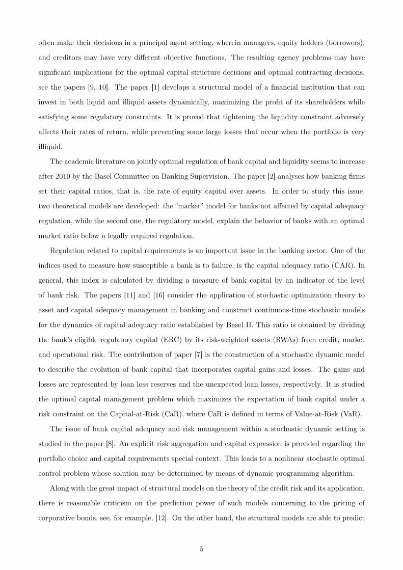
How CAR k∗ depends on the correlation ρ
Now we focus on the case of Vasicek distribution of the loan losses (1.7), which is characterized by
two parameters — ρ and PD — the borrower’s asset correlation and the probability of borrower’s
asset default, respectively. From intuitive point of view, the larger is correlation ρ, the more restrictive
banking policy is required. In other words, k∗(ρ) should be increasing function, but it is not clear,
whether the presented model catches this effect? The analytical way, like in Proposition 1, failed due
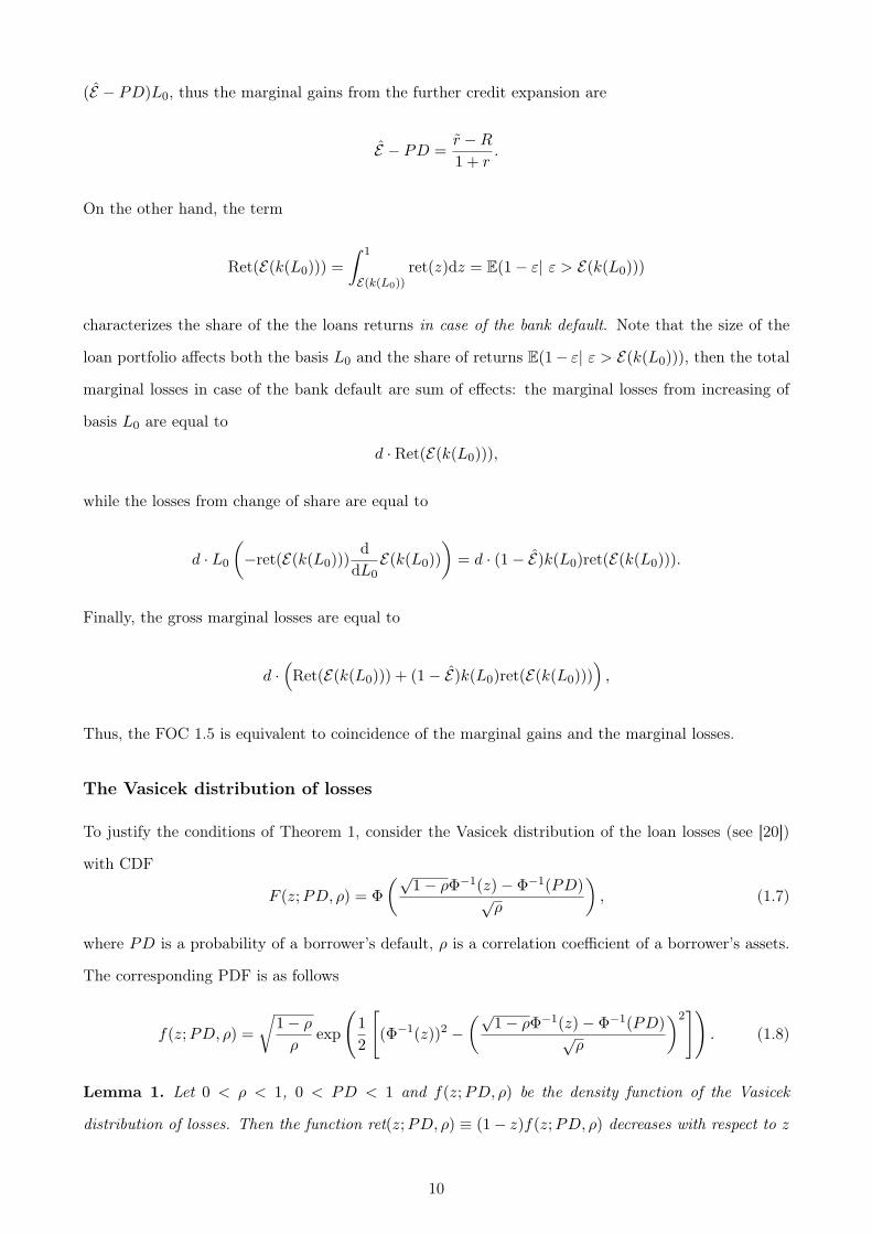
to very tedious calculations, thus, the Figures 1a and 1b show the series of computer simulations.
Figure 1a shows the curves, corresponding to the fixed discount d = 0.5 and three values of the default
probability PD = 0.06, 0.07, 0.08. Similarly, Figure 1b shows the curves, corresponding to the fixed
probability PD = 0.075 and three values of discount d = 0.3, 0.5, 0.75. As we see, increasing in both d
and PD shifts the curves upwards. An interpretation of this effect is quite natural. Increasing in both
cases implies the risk of default and/or the associated losses, which forces the “responsible” banker to
be more safe and conservative. Note that Figure 1b agrees with Proposition 1 statement on ∂k∗
∂d> 0.
2This statement was proved mostly by Dirk Tasche. Authors are grateful to him for the kind assistance.
11
a)
��=����
��=����
��=����
0.0 0.2 0.4 0.6 0.8 1.0
0.0
0.2
0.4
0.6
0.8
1.0
ρ
k*
b)
�=���
�=���
�=����
0.0 0.2 0.4 0.6 0.8 1.0
0.0
0.2
0.4
0.6
0.8
1.0
ρk
*
Figure 1: CAR k∗ as a function of ρ, R = 0.05, r = 0.15, a) d = 0.5, b) PD = 0.07
The lack of solution in neighborhood of ρ = 0 and ρ = 1 is result of violation of the solvability
condition (1.3). The direct calculations show that for all ρ sufficiently close to 0 or 1 the fraction
E − PD
Ret(E)
exceeds d = 0.5 and even it may be larger than 1. The values k∗ = 0, i.e., the bottom points of the
“arcs”, correspond to the threshold values of ρ, that satisfy the identity
E − PD
Ret(E ;PD, ρ)= d
and delimit the areas of ρ with the equilibrium with finite size of L∗0, which corresponds to the strictly
positive CAR k∗ > 0, from the “bubble” ρ with the unrestricted credit expansion L0 → ∞, which may
be associated with k∗ = 0. Therefore, we can extend the function k∗(ρ) on the “non-existence” areas
putting k∗(ρ) = 0.
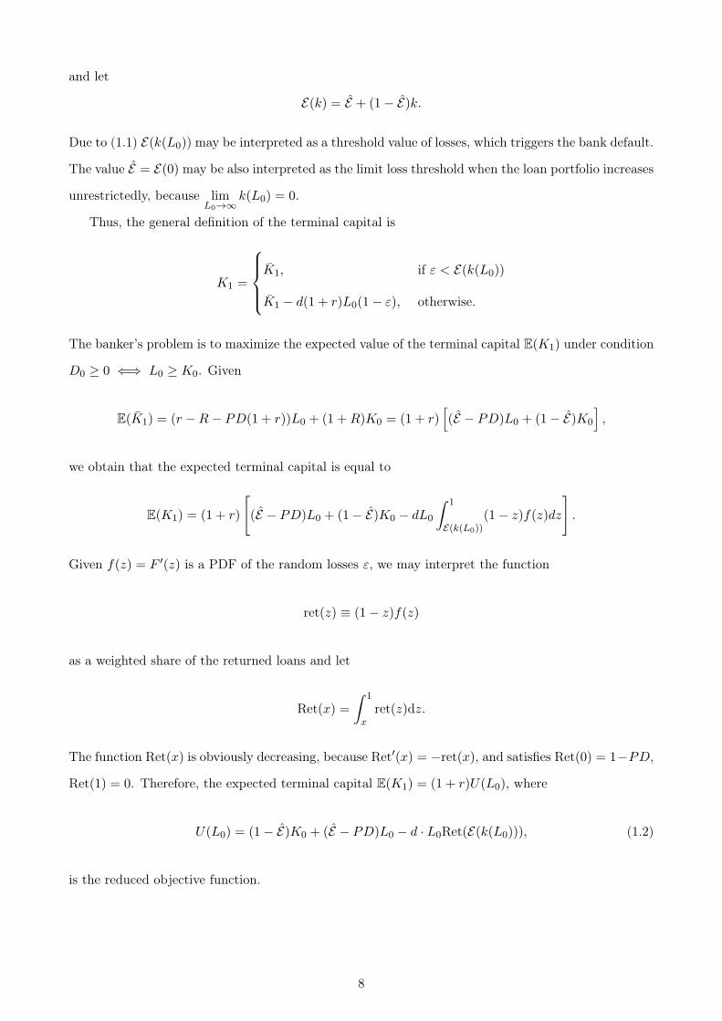
1.2 Probability of the bank’s default
The considered above optimum asset liability management is based on the risk-neutral behavior, tar-
geted to maximize the expected terminal capital E(K1), which is nominally greater than initial capital
K0, due to Theorem 1. However, the risk of default persists even if the management decisions are
optimal. The probability of event K1 ≤ 0 may be calculated as follows
p = P(ε ≥ E(k∗)) =∫ 1
E(k∗)f(z)dz = 1− F (E(k∗)), (1.9)
12
�
�*=�
��
�� �*>�
�*<�
0.0 0.2 0.4 0.6 0.8 1.0
0.0
0.2
0.4
0.6
0.8
1.0
ρ
p
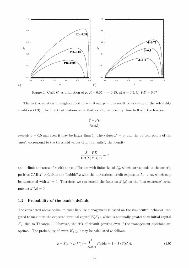
Figure 2: Probability of the banker’s default as function of ρ, d = 0.25, PD = 0.075
where k∗ is solution of equation (1.5). Function 1 − F (E(k)) strictly decreases with respect to k,
therefore, Proposition 1 implies that
∂p
∂d< 0,
∂p
∂R< 0,
∂p
∂r> 0,
which is quite intuitive. Note that the equilibrium values of k∗ must be positive, therefore, the feasible
values of the bank’s probability of default satisfy inequality p = 1− F (E(k∗)) < 1− F (E).
Focusing on the Vasicek distribution of losses, we can consider the comparative statics of probability
p with respect to specific parameters — the correlation ρ and the probability of borrower’s default PD.
Unfortunately, the analytic study of this question is problematic. The Figure 2 shows the result of the
computer simulations with d = 0.25, r = 0.15, R = 0.05, PD = 0.075.
Given the FOC
G(k, ρ) ≡ E − PD − d ·(
Ret(E(k); ρ) + (1− E)k · ret(E(k); ρ))
= 0,
13
we substitute k = F−1(1−p;ρ)−E1−E obtaining the equation
H(ρ, p) = G
(
F−1(1− p; ρ)− E1− E
, ρ
)
= 0,
which determines the implicit function p(ρ). The set of all solutions (ρ, p) of this equation contains
the “fictive” roots, violating the feasibility condition
k > 0 ⇐⇒ p(ρ) < 1− F (E , ρ).
To screen the fictive solutions we draw the delimiting border
k∗ = 0 ⇐⇒ p(ρ) = 1− F (E , ρ),
which is depicted by dashed curve on Figure 2. The solid curve P0P1 is a set of all feasible solution
(ρ, p), satisfying both H(ρ, p) = 0 and p(ρ) < 1−F (E , ρ) ⇐⇒ k∗ > 0. The points (ρ, p) of the pointed
curve above the border p = 1 − F (E , ρ), satisfying H(ρ, p) = 0 and p(ρ) > 1 − F (E , ρ) ⇐⇒ k∗ < 0,
are non-feasible.
As for definition of the default probability for ρ rightward to P1, let’s to recall that in these cases
the banker can not impose the self-restriction at some finite amount of the loan portfolio, which implies
L0 → ∞ ⇐⇒ k(L0) → 0. Thus we may define the function k(ρ) as folows
k∗(ρ) = 0 ⇒ p(ρ) = 1− F−1(
E ; ρ)
,
i.e., the continuation of the probability of the bank default belongs to the delimiting curve p = 1 −
F (E , ρ).
2 Parametric zoning by the solution types
The main aim of the present section is to visualize the various types of equilibria in terms of the model
primitives. First, assume that the deposit interest rate R, and CDF F (z) for the loan losses ε are
given and its PDF f(z) satisfies the condition ret(z) decreases for all PD < z < 1. Consider the set
S of feasible points r > R, 0 ≤ d ≤ 1 of the parameter plane (r, d). With any point of this set we
associate specific type of equilibrium, which corresponds to the whole set of parameters, including the
given ones. Figure 3 shows two examples of such zoning of S for the Vasicek distribution of losses,
which is characterized by two additional parameters, ρ and PD.
14

a)
���
0.00 0.05 0.10 0.15 0.20 0.25 0.30
r0.0
0.2
0.4
0.6
0.8
1.0
d
Figure 3: Vasicek distribution of loan losses: R = 0.1, PD = 0.04, ρ = 0.1
There are three, or, conditionally, four areas in parameters space, which may be described as
follows.
I. Bubble area B corresponds to the unrestricted credit expansion. It consists of points (r, d) ∈ S,
that violate condition (1.3).
II. Self-Constrained area S corresponds to case when the bank attracts deposits and places funds
to the loan portfolio of the limited size. It consists of points (r, d) ∈ S that satisfy conditions
(1.3) and r > R
III. Autarchy area A consists of points (r, d) ∈ S that satisfy the inequality r < R, 0 ≤ d ≤ 1, which
means that condition (1.3) trivially holds and the banker’s optimum solution is degenerate: the
bank does not attracts deposits, i.e., D0 = 0, while the the loan portfolio L0 = K0 > 0.
Remark 3. For any given positive value of discount d+ > 0, no matter how small is it, we obtain
the nonempty intersection of the line d = d+ with all three areas. If d = 0, that corresponds to the
linear model of Section 1, the Self-Constrained area S vanishes and we obtain only two generic cases
—Bubble area B and Autarchy area A, which agrees with result obtained in Section 1.
The main result of this subsection is that the shapes of this zoning does not depend, on choice of
distribution function
Proposition 2. The structure of areas B, S, A is persisting.
Proof. See Appendix A.4.
2.1 The Basel III requirements
The Basel III requires that the probability of the bank’s default
p = 1− F (E(k∗))
15
must not exceed 0.001, which implies the inequality
k∗ ≥ k =VaR99.9 − E
1− E.
where VaR99.9 = F−1(0.999).
The Basel III analysis uses the Vasicek loan losses distribution (1.7), therefore,
VaR99.9 = F−1(0.999;PD, ρ) = Φ
(√
ρ
1− ρΦ−1(0.999) +
√
1
1− ρΦ−1(PD)
)
, (2.1)
which allows to calculate the corresponding required value of CAR. Now we are going to identify sets of
the bank parameters d, r, R, PD, ρ which guarantee that the banker complies voluntarily with Basel III
requirements, or, on the contrary, the external regulation is needed. Substituting VaR99.9 = E(k) into
equation (1.5), we can determine the minimum value of discount dB, as a function of r, guaranteeing
the precise discharge of Basel III requirements, as follows
dB(r) =E − PD
Ret(VaR99.9) + (VaR99.9 − E)ret(VaR99.9). (2.2)
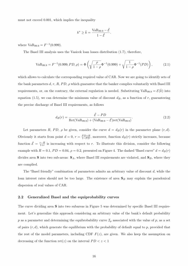
Let parameters R, PD, ρ be given, consider the curve d = dB(r) in the parameter plane (r, d).
Obviously it starts from point d = 0, r = PD+R1−PD
, moreover, function dB(r) strictly increases, because
function E = r−R1+r
is increasing with respect to r. To illustrate this division, consider the following
example with R = 0.1, PD = 0.04, ρ = 0.2, presented on Figure 4. The dashed “Basel curve” d = dB(r)
divides area S into two sub-areas: SA, where Basel III requirements are violated, and SB, where they
are complied.
The “Basel friendly” combination of parameters admits an arbitrary value of discount d, while the
loan interest rates should not be too large. The existence of area SB may explain the paradoxical
dispersion of real values of CAR.
2.2 Generalized Basel and the equiprobability curves
The curve dividing area S into two subareas in Figure 5 was determined by specific Basel III require-
ment. Let’s generalize this approach considering an arbitrary value of the bank’s default probability
p as a parameter and determining the equibrobability curve Ip associated with the value of p, as a set
of pairs (r, d), which generate the equilibrium with the probability of default equal to p, provided that
the rest of the model parameters, including CDF F (z), are given. We also keep the assumption on
decreasing of the function ret(z) on the interval PD < z < 1
16

�����
0.16 0.18 0.20 0.22 0.24
r0.0
0.2
0.4
0.6
0.8
1.0
d
Figure 4: Dichotomy “self-restriction – external restriction”
Theorem 2. The assemblage of curves Ip is characterized by the following properties:
1. All curves Ip associated with different probabilities p start from the same point r = R+PD1−PD
, d = 0.
2. If probability of the bank’s default p converges to zero, then the curves Ip converge to the vertical
line r = R+PD1−PD
, 0 ≤ d ≤ 1.
3. The assemblage of curves Ip for all p < 1 − F (PD) fills the whole Self-Constrained area S,
moreover, for p < p′ the curve Ip resides leftward and above the curve Ip′ .
4. For all sufficiently small p the equiprobability curve Ip does not intersect the border of the areas
B and S for 0 < d ≤ 1.
Proof. See Appendix A.5.
Figure 5 illustrates the three possible cases of the equiprobability curves described in Theorem 2
for the Vasicek distribution of losses with PD = 0.04, ρ = 0.2, and R = 0.1. Solid curve is the border
between Self-Constrained and Bubble areas, while three dashed lines are the equiprobability curves Ipassociated with three values of the bank probability of default: for the very large probability p = 0.25
the curve Ip leave the Self-Constrained area immediately, for the intermediate value p = 0.05 the curve
Ip intersect the border, while the small probability of the bank default p = 0.02 generates the curve
Ip intersecting the line d = 1.
17

BS
p=0.25
p=0.05
p=0.02
0.16 0.18 0.20 0.22 0.24
r0.0
0.2
0.4
0.6
0.8
1.0
d
Figure 5: Equiprobability curves Ip for p = 0.02, 0.05, 0.25.
3 Conclusion
The banking is one of the most over-regulated and over-supervised industries, and the pressure on
banks continues to grow. A natural question arises: can banks do without a regulator - at least in
some aspects of their activities that are now under strict regulation and supervision?
For example, can banks limit their credit expansion on their own, without intervention of a regula-
tor? To answer this question, we built a simple microeconomic model with one stochastic factor – the
share of non-performing loans. It turned out that if, in the event of a bank default, a loan portfolio
can be sold without a discount, then the banker has no incentives to limit the credit expansion, even
despite the prospect of incurring of huge losses. This means that in this case, banking cannot do
without a regulator, only the state can restrict the credit expansion.
The situation changes drastically, when we assume that in the event of a bank failure, its loan port-
folio is sold at some non-zero discount. In this case, when certain limitations on the model parameters
are satisfied, an endogenous restriction of credit expansion arises. Unlike external restrictions that
banks have learned to successfully circumvent, these restrictions are internal, and deceiving oneself is
usually not beneficial. However, from the point of view of the regulator, which evaluates the result in
terms of CAR, the level of bank self-restraint may seem unacceptable, for example, if the ratio has a
too low value. In this paper we derive the conditions of the existence and uniqueness of equilibrium
(FOC and SOC), which have the clear economic interpretation and appropriate for both analytical and
numerical study.
There is a problem of identifying the outcome in terms of the basic parameters of the model. This
18
task received a comprehensive solution. A procedure has been formulated and justified, which makes
it possible to unambiguously determine the type of outcome according to the model exogenous param-
eters and the known loss distribution function. It was shown that with sufficiently weak and natural
restrictions on the loss distribution function, that the parameter space is divided into 3 non-empty
regions in which one of the three possible outcomes is realized: B (“Bubble”) - there are no bounded
solutions (i.e., we get an analogue of the linear model with zero discount); S (“Self-Constraned”) with
limited solutions; and, finally, A - autarchy solutions - deposits are not attracted, loans are placed
within their own funds as a result, credit expansion does not occur due to unfavorable conditions. In
addition, a more subtle identification of compliance with the requirements established by Basel III in
the area S was carried out.
The influence of exogenous factors on solutions, both analytically and, in particularly complex cases,
using computer simulations, has been studied. In all cases, the results of the study of comparative
statics are consistent with intuitive expectations.
References
[1] Astic, F., and Tourin, A., “Optimal bank management under capital and liquidity constraints”,
Journal of Financial Engineering, vol. 0, no. 03, September 2014
[2] Barrios, V.E., and Blanco, J.M., The effectiveness of bank capital adequacy regulation: A theo-
retical and empirical approach, Journal of Banking & Finance 27 (2003) 1935–1958
[3] BIS (2019), IRB approach: risk weight functions – January
[4] BIS (2019), BIS Annual Economic Report 2019 - June
[5] Black F, Cox J.C. 1976. Valuing corporate securities: some effects of bond indenture provisions.
J. Finance 31:351–67
[6] Black F, Scholes M. 1973. The pricing of options and corporate liabilities. J. Polit. Econ. 81:637–54
[7] T. Bosch, J. Mukuddem-Petersen, M.P. Mulaudzi and M.A. Petersen, “Optimal Capital Manage-
ment in Banking”, Proceedings of the World Congress on Engineering 2008 Vol II WCE 2008, July
2 - 4, 2008, London, U.K.
[8] F. Chakroun and F. Abid, “Capital adequacy and risk management in banking industry”, Applied
Stochastic Models in Business and Industry, vol. 32, no. 1, 113-132, 2016.
19
[9] DeMarzo P, Fishman M. 2007a. Agency and optimal investment dynamics. Rev. Financ. Stud.
20:151–88
[10] DeMarzo P, Sannikov Y. 2006. Optimal security design and dynamic capital structure in a
continuous-time agency model. J. Finance 61:2681–724
[11] Fouche, C.H., Mukuddem-Petersen J. and Petersen M.A., Continuous-timestochastic modelling
of capital adequacy ratios for banks. Applied Stochastic Models in Business and Industry 2006;
22(1):41-71.
[12] Huang, J. and M. Huang, 2012, How much of the corporate-treasury yield spread is due to credit
risk?, Review of Asset Pricing Studies 2.2, 153-202.
[13] Leland H. 1994. Corporate debt value, bond covenants, and optimal capital structure. J. Finance
49:1213–52
[14] Leland, H., 2004. Predictions of default probabilities in structural models of debt. Journal of
Investment Management 2, 5–20.
[15] Merton, R.C., (1974), On the pricing of corporate debt: the risk structure of interest rates. J.
Finance 29:449–70
[16] J. Mukuddem-Petersen and M.A. Petersen, Optimizing Asset and Capital Adequacy Management
in Banking, J. Optim. Theory Appl. (2008) 137: 205–230
[17] Reinhart, C. M. and Rogoff, K. S.: (2009) This Time Is Different: Eight Centuries of Financial
Folly, Princeton University Press
[18] Schaefer SM, Strebulaev I. 2008. Structural models of credit risk are useful: evidence from hedge
ratios on corporate bonds. J. Financ. Econ. 90:1–19
[19] Vasicek O., (1987): Probability of Loss on Loan Portfolio, KMV Corporation
[20] Vasicek O., (2002): The Distribution of Loan Portfolio Value, Risk, December, 160-162
20
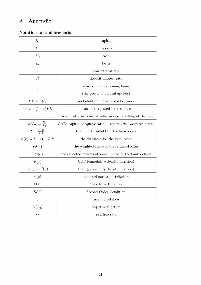
A Appendix
Notations and abbreviations
Kt capital
Dt deposits
Mt cash
Lt loans
r loan interest rate
R deposit interest rate
εshare of nonperforming loans
(the portfolio percentage loss)
PD = E(ε) probability of default of a borrower
r = r − (1 + r)PD loan risk-adjusted interest rate
d discount of loan nominal value in case of selling of the loan
k(L0) =K0
L0CAR (capital adequacy ratio) – capital/risk weighted assets
E = r−R1+r
the limit threshold for the loan losses
E(k) = E + (1− E)k the threshold for the loan losses
ret(z) the weighted share of the returned loans
Ret(E) the expected returns of loans in case of the bank default
F (x) CDF (cumulative density function)
f(x) = F ′(x) PDF (probability density function)
Φ(z) standard normal distribution
FOC First-Order Condition
SOC Second-Order Condition
ρ asset correlation
U(L0) objective function
rf risk-free rate
21

A.1 Proof of Theorem 1
Proof. Differentiating the function (1.2), we obtain the derivatives
U ′(L0) = E − PD − d ·(
Ret(E(k(L0))) + (1− E)k(L0)ret(E(k(L0)))
(A.1)
U ′′(L0) = −d ·[
−ret(E(k(L0))dEdL0
+ (1− E)ret(E(k(L0))dk
dL0+ (1− E)k(L0)ret
′(E(k(L0))dEdL0
]
=
=d
L0· (1− E)2k2(L0)ret
′(E(k(L0)) < 0. (A.2)
Furthermore,
U ′(K0) = E − PD − d (1− F (1)− PD + Ret(0)) = E − PD > 0,
limL0→∞
U ′(L0) = E − PD − d · Ret(E).
Given the SOC U ′′ < 0, we obtain that a necessary and sufficient condition for the existence and
uniqueness of the FOC U ′(L0) = 0 is the inequality
limL0→∞
U ′(L0) < 0 ⇐⇒ d >E − PD
Ret(E).
Due to (A.1) we may represent the FOC U ′(L0) = 0 as the equation
E − PD − d ·(
Ret(E(k)) +(
1− E)
k · ret(E(k)))
= 0
of variable k = K0/L0, which sets the correspondence between solution of this equation k∗ and the
equilibrium size of the loan portfolio L∗0.
Q.E.D.
A.2 Proof of Lemma 2
Assume first that ρ < 1/2 and PD ≤ 1/2 , then in this case the PDF (1.8) is unimodal with mode at
zmode = Φ
(√1− ρ
1− 2ρΦ−1(PD)
)
,
(see, e.g., [20]). Moreover, ρ < 1/2 and PD ≤ 1/2 imply
√1− ρ
1− 2ρ> 1 ⇒
√1− ρ
1− 2ρΦ−1(PD) ≤ Φ−1(PD) ⇒ zmode ≤ Φ(Φ−1(PD)) = PD,
because Φ−1(PD) ≤ 0, therefore, f(z) decreases with respect to z, as well as (1− z)f(z) does.
22
Now assume that 1 > ρ ≥ 1/2 and PD ≤ 1/2. Substituting x = Φ−1(z) we obtain the following
problem: to prove that the function
h(x) =
√
1− ρ
ρexp
(
1
2
[
x2 −(√
1− ρx− c√ρ
)2])
(1− Φ(x)) = ϕ
(√1− ρx− c√
ρ
)
Φ(−x)
ϕ(x)
is decreasing with respect to x, where c = Φ−1(PD) < 0, ϕ(z) = Φ′(z) > 0 is the density function
of the standard normal distribution satisfying the identity ϕ′(x) = −xϕ(x). Differentiating h(x) we
obtain
h′(x) =ϕ(√
1−ρx−c√ρ
)
ϕ(x)
[(
c√1− ρ
ρ+
2ρ− 1
ρx
)
Φ(−x)− ϕ(x)
]
.
Assume first that x ≤ 0. Given c = Φ−1(PD) ≤ 0, we obtain
(
c√1− ρ
ρ+
2ρ− 1
ρx
)
Φ(−x)− ϕ(x) < 0 ⇒ h′(x) < 0.
Now let x > 0, then
(
c√1− ρ
ρ+
2ρ− 1
ρx
)
Φ(−x)− ϕ(x) < xΦ(−x)− ϕ(x) < 0,
due to
2ρ− 1
ρ= 1− 1− ρ
ρ< 1
and ϕ(x) > xΦ(−x) for all x ≥ 0. Indeed, ϕ(0) > 0 = 0 · Φ(−0) and for all x > 0 the inequality
ϕ′(x) = −xϕ(x) = −xϕ(−x) > Φ(−x)− xϕ(−x) = (xΦ(−x))′
holds, which completes the proof of this case.
Finally, assume that PD > 1/2, then c = Φ−1(PD) > 0, and z > PD implies x = Φ−1(z) > c > 0
and, consequently,
c√1− ρ
ρ+
2ρ− 1
ρx <
2ρ− 1 +√1− ρ
ρx = x−
√1− ρ(1−√
1− ρ)
ρx < x
for all 0 < ρ < 1. The rest of proof is similar. Q.E.D.
23

A.3 Proof of Proposition 1
To simplify calculations, consider the following substitution of variables E = E + (1 − E)k. Then the
FOC (1.5) is equivalent to the equation
G(E) ≡ E − PD − d ·(
Ret(E) +(
E − E)
ret(E))
= 0.
Let E∗ be the solution of this equation, considered as an implicit function of all parameters. The
corresponding derivative with respect to an arbitrary parameter a is as follows
∂E∗
∂a= −∂G
∂a
/∂G
∂E,
where
∂G
∂E= d ·
(
E − E)
(f(E)− (1− E)f ′(E)) = −d ·(
E − E)
ret′(E) > 0,
because E > E and ret(E) is a decreasing function. Moreover,
∂G
∂d= −
(
Ret(E) +(
E − E)
ret(E))
< 0,
which implies ∂E∗
∂d> 0.
Now let a = R, given
E =r −R
1 + r
we obtain
∂G
∂R= − 1
1 + r− d · ret(E)
1 + r< 0,
which implies ∂E∗
∂R> 0. Furthermore, the inequality
∂G
∂r=
1 +R
(1 + r)2+ d · (1 +R)ret(E)
(1 + r)2> 0
implies ∂E∗
∂r< 0.
Given E∗ = (1− E)k∗ + E and E = r−R1+r
, we obtain that
k∗ =(1 + r)E∗ − (r −R)
1 +R, L∗
0 =(1 +R)K0
(1 + r)E∗ − (r −R), D∗
0 = L∗0 −K0,
therefore,
∂k∗
∂d> 0,
∂L∗0
∂d< 0,
∂D∗0
∂d< 0
24

Moreover,
∂k∗
∂R= − 1 + r
(1 +R)2E∗ +
1 + r
1 +R
∂E∗
∂R+
1 + r
(1 +R)2=
1 + r
(1 +R)2(1− E∗) +
1 + r
1 +R
∂E∗
∂R> 0,
∂L∗0
∂R=
∂D∗0
∂R=
K0 ((1 + r)E∗ − (r −R))− (1 +R)K0
(
(1 + r)∂E∗
∂R+ 1)
((1 + r)E∗ − (r −R))2=
=− (1 + r)K0
(
(1− E∗) + (1 +R)∂E∗
∂R
)
((1 + r)E∗ − (r −R))2< 0,
because E∗ < 1 , ∂E∗
∂R> 0.
Finally,
∂k∗
∂r=
1
1 +R
[
(1 + r)∂E∗
∂r− (1− E∗)
]
< 0
∂L∗0
∂r=
∂D∗0
∂r= − (1 +R)K0
((1 + r)E∗ − (r −R))2
[
E∗ − 1 + (1 + r)∂E∗
∂r
]
> 0,
because of E∗ < 1 and ∂E∗
∂r< 0. Q.E.D.
A.4 Proof of Proposition 2
The statement about area A is obvious. The rest is to show the robustness of shapes of areas B and
S. Note that the function
dS(r) =E(r)− PD
Ret(E(r)),
where E(r) = r−R1+r
, satisfies the following conditions:
1. dS
(
PD+R1−PD
)
= 0,
2. dS (r) strictly increases for all r > PD+R1−PD
.
The first statement is obvious by due to definition of dS (r). Then, representing the function dN (r) as
follows
dS(r) =r −R
1 + r· 1
Ret(
r−R1+r
) ,
and given the functions r−R1+r
, r−R1+r
are positive and strictly increasing with respect to r we obtain that
the function d0(r) is also strictly increasing. Finally, the function dS (r) is unrestrictedly increasing
with r → ∞, because
r −R
1 + r→ 1− PD,
r −R
1 + r→ 1.
Therefore, its graph intersects the line d = 1 in finite point rS > PD+R1−PD
, which determine the base of
25
the curvilinear triangle S. Q.E.D.
A.5 Proof of Theorem 2
Consider the probability of the bank’s default p as a parameter with possible values from the interval
[0, 1]. Formula (1.9) implies that for any given p, the equation p = 1 − F (E) determines the value
Ep = F−1(1− p). This means that the equiprobability curve Ip is determined by equation
E(r)− PD − d ·(
Ret(Ep) +(
Ep − E(r))
ret(Ep))
= 0,
or, equivalently,
d = dp(r) ≡E(r)− PD
Ret(Ep) +(
Ep − E(r))
ret(Ep), (A.3)
where E(r) = r−R1+r
. It is obvious that dp
(
PD+R1−PD
)
= 0 for all p, which completes the first statement of
the theorem. Moreover, p → 0 implies Ep → 1, therefore, limp→0
dp(r) = +∞ for any r > R+PD1−PD
⇐⇒
E(r)− PD > 0, which completes the second statement.
Recall that the border of areas S and B is determined by the function
dS (r) =E(r)− PD
Ret(E(r)).
Calculating and comparing the derivatives of dS(r) and dp(r) at the starting point r0 =R+PD1−PD
d
drdS(r0) =
(1− PD)2
(1 +R)Ret(PD),
d
drdp(r0) =
(1− PD)2
(1 +R) (Ret(Ep) + (Ep − PD)ret(Ep)),
we obtain that
d
drdp(r0) >
d
drdS(r0) ⇐⇒ Ret(PD) > Ret(Ep) + (Ep − PD)ret(Ep).
Consider the function
G(x) = Ret(x) + (x− PD)ret(x),
which obviously satisfies G(PD) = Ret(PD). Moreover,
G′(x) = (x− PD)ret′(x) < 0
26

for all x > PD. This implies that
x = Ep = F−1(1− p) > PD ⇐⇒ p < 1− F (PD)
is necessary and sufficient condition for the curve Ip to belong the area S, at least in some neighborhood
of r0.
Let’s determine the point of intersection of the equiprobability curve Ip with the border of areas S
and B from the following equation
dS(r) = dP (r) ⇐⇒ Ret(E(r)) = Ret(Ep) +(
Ep − E(r))
ret(Ep).
The unique solution r(p) of this equation is determined by identity
Ep = E(r(p)) ⇐⇒ r(p) =Ep +R
1− Ep=
F−1(1− p) +R
1− F−1(1− p)> r0 =
PD +R
1− PD
because F−1(1− p) > PD. Note that this point of intersection is actual only in case
dS(r(p)) = dp(r(p)) ≤ 1,
otherwise, the equiprobability curve will intersect the line d = 1 instead of dS(r). This happens if and
only if
dS(r(p)) > 1 ⇐⇒ Ep − PD − Ret(Ep) > 0.
Note that the function
H(x) = x− PD − Ret(x)
for x ≥ PD satisfies the following conditions: H(PD) < 0, H(1) = 1 − PD > 0, and H ′(x) =
1 + (1 − x)f(x) > 0. This implies that there is x∗ ∈ (PD, 1) such that for all x > x∗ the function
H(x) > 0, which is equivalent to
p < 1− F (x∗) ⇒ Ep − PD − Ret(Ep) > 0.
Q.E.D.
27