Welcome to BS6207

2021 Lee Hwee Kuan

1

Adjustment to Grading

1. 10% class participation How to assign grades?

2. 45% assignments 4 x reports: 35% (8+8+8+11) Presentation 10% (5+5) - 2 presentations per student, not the whole assignment

3. 45% project Report 30% Presentation 15% - lead presenter, 2 students assist

2

Assignment of class participation grades

3 times 1% — total 30 times

3

Assignment due dates, Fridays 18:30 hours

Assignment #1: 5th week I will post new assignment by coming Monday

Assignment #2: 6th week - post by 5th week Assignment #3: 7th week - post by 6th week Assignment #4: 8th week - post by 7th week

Assignment presentations: Assignment #1: 6th week Wed 4 students Assignment #2: 7th week Wed 4 students Assignment #3: 8th week Wed 4 students Assignment #4: 9th week Wed 4 students

4

Project due date Week #8: first report submission

- baseline model and to show that you started the project Week #11: final report Friday 18:30 hours

Project presentations Week #12 &13

5

Short review

6

Basic construction of neural networks

x1

x2

b(2)

w(2)1

w(2)2

b(1)w(1)

1

w(1)2

o

h(2)

h(1)

w(3)1

w(3)2

o = �(w(3)1 h(1) + w(3)

2 h(2) + b(3))

h(1) = �(w(1)1 x1 + w(1)

2 x2 + b(1))

h(2) = �(w(2)1 x1 + w(2)

2 x2 + b(2))

7

Basic construction of neural networks

x1。 。 。

xd

h(1)

。 。 。

h(k)

h(1) = �(~w1 · ~x+ b1)

h(k) = �(~wk · ~x+ bk)

h̃(j) = �(~wj · ~h+ bj)

。 。 。

h̃(1)

h̃(j)

。 。 。

。 。 。

8

oxx 2 R

Role of parameters andw b

o =1

1 + exp(�wx� b)

-10 -5 0 5 10x

0

0.2

0.4

0.6

0.8

1

σ

w = 1, b = 0w = 2, b = 0w = 0.5, b = 0

-10 -5 0 5 10x

0

0.2

0.4

0.6

0.8

1

σ

w = 1, b = +5, b/w = 5w = 1, b = -5, b/w = -5w = 2, b = -5, b/w = -2.5w = 2, b = -10, b/w = -5

9

Role of parameters andw b

Do it yourself : plot ReLU graph for various w b

10

Function picture of network

11

x1

x2

o

x1

x2

x1

x2

level sets form straight lines

12

x1

x1

x2

x2x2

x1

+

h2(x1, x2)h1(x1, x2)

x1x2

+

�h3(x1, x2)

Function view of neural network

13

Manifold view of neural network

14

Matrix notation

15

h1,i = �

0

@X

j

W (0,1)j,i xj + bi

1

A i = 1, · · ·

element wise operation

�[(z1, z2, z3, · · · )] = (�(z1),�(z2),�(z3))

~h1 = �[W (0,1) · ~x+~b1]

~b1 ~b2 ~b3

~h1~h2

~h3 = o~x

W (0,1) W (1,2) W (2,3)

16

~h2 = �[W (1,2) · ~h1 +~b2]

~h1 = �[W (0,1) · ~x+~b1]

~b1 ~b2 ~b3

~h1~h2

~h3 = o~x

W (0,1) W (1,2) W (2,3)

~h3 = �[W (2,3) · ~h2 +~b3]

�[(z1, z2, z3, · · · )] = (�(z1),�(z2),�(z3))

17

Activation functions

18

so many examples in https://en.wikipedia.org/wiki/Activation_function

Soft plus f(z) = ln(1 + exp(z))

Rectified linear f(z) = max(0, z)

Sigmoid f(z) =1

1 + exp(�z)

f(z) = tanh(z)Hyperbolic tangent

-10 -5 0 5 10Z

0

0.2

0.4

0.6

0.8

1

f(z)

-10 -5 0 5 10Z

0

2

4

6

8

10

f(z)

-10 -5 0 5 10Z

0

2

4

6

8

10

f(z)

-10 -5 0 5 10Z

-1-0.8-0.6-0.4-0.20

0.20.40.60.81

f(z)

[-1,1]

[0,1]

[0,inf]

[0,inf]

19

Cost function

20

Square error

l(yi, oi) = kyi � oik2Given data points (xi, yi), i = 1, · · ·n

C =1

n

X

i

l(yi, oi)

xn, xn�1, · · ·x2, x1

o1, y1

o2, y2...

on, yn

Adjust the weights until C = 0 (or close to zero)

21

C = � 1n

Pi yi log[o(xi)] + (1� yi) log[1� o(xi)]

C =1

n

X

i

l(yi, oi)

Cross entropy cost function

l(yi, oi) = yi · log(oi)

yi 2 {0, 1}

yi 2 {(1, 0, 0), (0, 1, 0), (0, 0, 1)}Three class example

Two class example

. . . v1v2v3

output

m = exp(v1) + exp(v2) + exp(v3)

oi = (exp(v1)

m,exp(v2)

m,exp(v3)

m)

22

23

Loss function is a surfaceconsider 4 data points x1 = 0.1, y1 = 0 x2 = 0.2, y2 = 0 x3 = 0.6, y3 = 1 x4 = 0.9, y4 = 1

ox w

b=-0.5

o =1

1 + exp(�wx)Table 1

w x1 o1 y1 x2 o2 y2 x3 o3 y3 x4 o4 y4 Loss

-2 0.1 0.33 0 0.2 0.29 0 0.6 0.15 1 0.9 0.09 1 1.7436-1.5 0.1 0.34 0 0.2 0.31 0 0.6 0.20 1 0.9 0.14 1 1.5913-1 0.1 0.35 0 0.2 0.33 0 0.6 0.25 1 0.9 0.20 1 1.4339

-0.5 0.1 0.37 0 0.2 0.35 0 0.6 0.31 1 0.9 0.28 1 1.25390 0.1 0.38 0 0.2 0.38 0 0.6 0.38 1 0.9 0.38 1 1.0576

0.5 0.1 0.39 0 0.2 0.40 0 0.6 0.45 1 0.9 0.49 1 0.87471 0.1 0.40 0 0.2 0.43 0 0.6 0.52 1 0.9 0.60 1 0.7353

1.5 0.1 0.41 0 0.2 0.45 0 0.6 0.60 1 0.9 0.70 1 0.62062 0.1 0.43 0 0.2 0.48 0 0.6 0.67 1 0.9 0.78 1 0.5726

24

Table 1

w x1 o1 y1 x2 o2 y2 x3 o3 y3 x4 o4 y4 Loss

-2 0.1 0.33 0 0.2 0.29 0 0.6 0.15 1 0.9 0.09 1 1.7436-1.5 0.1 0.34 0 0.2 0.31 0 0.6 0.20 1 0.9 0.14 1 1.5913-1 0.1 0.35 0 0.2 0.33 0 0.6 0.25 1 0.9 0.20 1 1.4339

-0.5 0.1 0.37 0 0.2 0.35 0 0.6 0.31 1 0.9 0.28 1 1.25390 0.1 0.38 0 0.2 0.38 0 0.6 0.38 1 0.9 0.38 1 1.0576

0.5 0.1 0.39 0 0.2 0.40 0 0.6 0.45 1 0.9 0.49 1 0.87471 0.1 0.40 0 0.2 0.43 0 0.6 0.52 1 0.9 0.60 1 0.7353

1.5 0.1 0.41 0 0.2 0.45 0 0.6 0.60 1 0.9 0.70 1 0.62062 0.1 0.43 0 0.2 0.48 0 0.6 0.67 1 0.9 0.78 1 0.5726

0

0.45

0.9

1.35

1.8

-2 -1.5 -1 -0.5 0 0.5 1 1.5 2

w

cost

(s

quar

e er

ror )

C(w1, w2) =1

n

X

i

l(yi, oi) + 0.2(w21 + w2

2)

w1w2

cost

x1

x2

ow2

w1 b=0l(yi, oi) = kyi � oik2

25

How to adjust the weights?

Conceptually, this will work:

Try all possible weights combinations, for all weights combinations, calculate the cost for all combinations. Then pick the weight combination that has the lowest cost.

Practically, there are too many weights combinations to try.

26

Back propagation and gradient descend

27

28

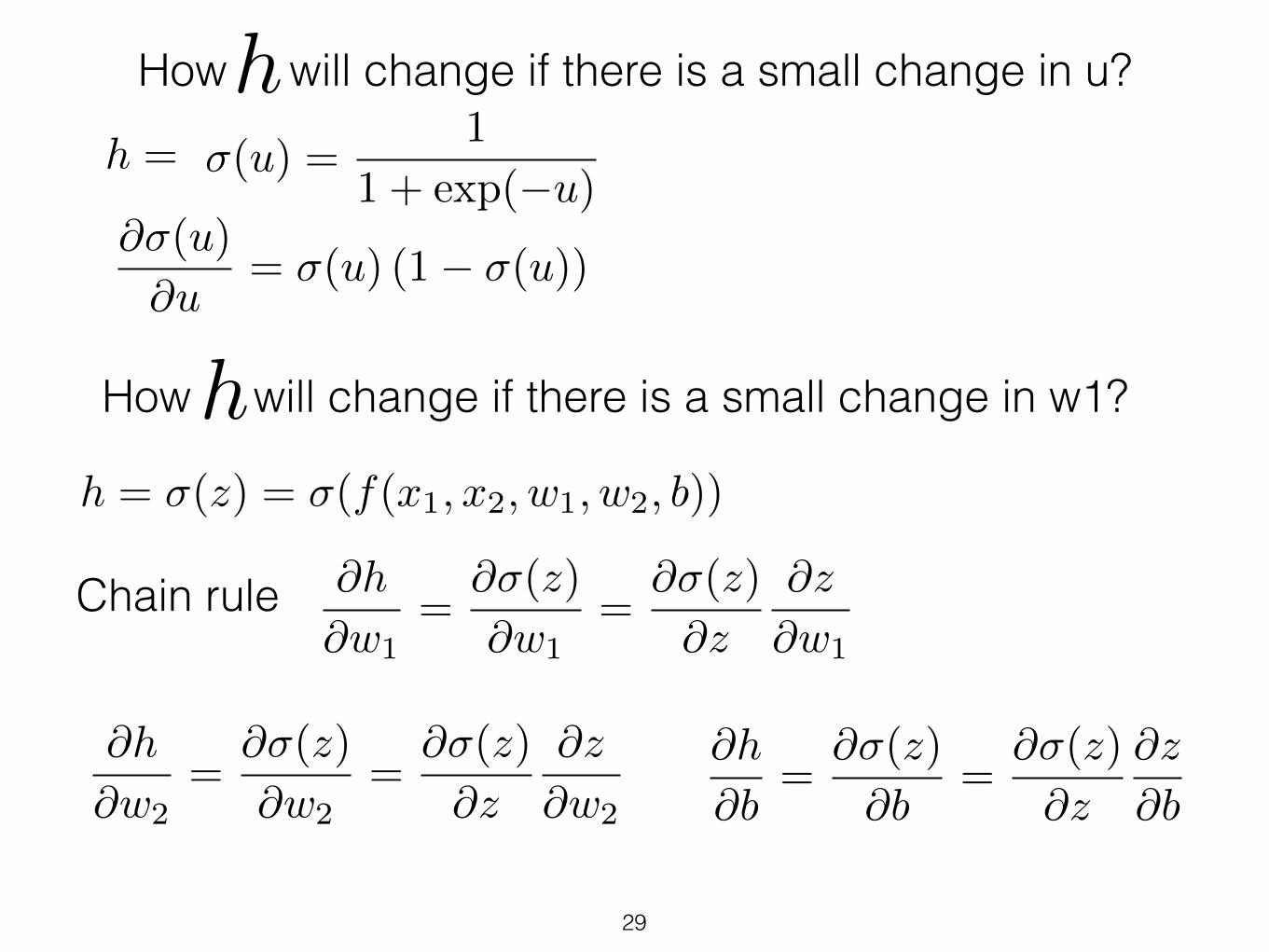
Basic calculus required for understanding backpropagation

Composite function

�(u) =1

1 + exp(�u)

f(x1, x2, w1, w2, b) = w1x1 + w2x2 + b

f(x1, x2, w1, w2, b) = z = w1x1 + w2x2 + b

z �

h = �(f(x1, x2, w1, w2, b))

h

29

�(u) =1

1 + exp(�u)h =

How will change if there is a small change in u?h

@�(u)

@u= �(u) (1� �(u))

Chain rule

How will change if there is a small change in w1?hh = �(z) = �(f(x1, x2, w1, w2, b))

@h

@w1=

@�(z)

@w1=

@�(z)

@z

@z

@w1

@h

@w2=

@�(z)

@w2=

@�(z)

@z

@z

@w2

@h

@b=

@�(z)

@b=

@�(z)

@z

@z

@b

x1

x2

w1

w2

b

z � hf

@h

@w1=

@�(z)

@w1=

@�(z)

@z

@z

@w1

@h

@w2=

@�(z)

@w2=

@�(z)

@z

@z

@w2

@h

@b=

@�(z)

@b=

@�(z)

@z

@z

@b

31

�

x1

x2

w1 +�w1

w2

b

z +�z h+�h

@h

@w1=

@�(z)

@w1=

@�(z)

@z

@z

@w1

@h

@w2=

@�(z)

@w2=

@�(z)

@z

@z

@w2

@h

@b=

@�(z)

@b=

@�(z)

@z

@z

@b

f

Gradient descend

x w1 w2 w2v1 v2 v3w3

v3 = �(z3) = �(w3v2 + b3)

v2 = �(z2) = �(w2v1 + b2)

v1 = �(z1) = �(w1x+ b1)

@C

@wj= 0

@C

@bj= 0

32

We just need @oi@wj

@C

@wj= 0

@C

@bj= 0

wj(t+ 1) = wj(t)� ⌘@C

@wj

@C

@wj=

1

n

X

i

@(yi � oi)2

@wj

= � 2

n

X

i

(yi � oi)@oi@wj

33

x w1 w2 w2v1 v2 v3w3 = o

v3 = �(z3) = �(w3v2 + b3)

v2 = �(z2) = �(w2v1 + b2)

v1 = �(z1) = �(w1x+ b1)

@v3@w3

=@v3@z3

@z3@w3

= �0(z3)v2

@v3@w2

=@v3@z3

@z3@w2

= �0(z3)w3@v2@w2

= �0(z3)w3�0(z2)v1

@v3@w1

=@v3@z3

@z3@w1

= �0(z3)w3@v2@w2

= �0(z3)w3�0(z2)w2

@v1@w1

= �0(z3)w3�0(z2)w2�

0(z1)x

34

x w1 w2 w2v1 v2 v3w3 = o@v3@w3

=@v3@z3

@z3@w3

= �0(z3)v2

@v3@w2

=@v3@z3

@z3@w2

= �0(z3)w3@v2@w2

= �0(z3)w3�0(z2)v1

@v3@w1

=@v3@z3

@z3@w1

= �0(z3)w3@v2@w2

= �0(z3)w3�0(z2)w2

@v1@w1

= �0(z3)w3�0(z2)w2�

0(z1)x

problem!! : long mathematical expression leads to large computational time for deep network

35

x w1 w2 w2v1 v2 v3w3 = o

Compute and store strategy

@v3@z3

= �0(z3)

@v3@z2

=@v3@z3

@z3@z2

=@v3@z3

w3�0(z2)

@v3@z3

@v3@z2

@v3@z1

=@v3@z2

@z2@z1

=@v3@z2

w2�0(z1)

@v3@z1

36

x w1 w2 w2v1 v2 v3w3 = o

Compute and store strategy

@v3@z3

@v3@z2

@v3@z1

@v3@w3

=@v3@z3

@z3@w3

=@v3@z3

v2

@v3@w2

=@v3@z2

@z2@w2

=@v3@z2

v1

please work this out

@v3@bj

?

@v3@w1

=@v3@z1

@z1@w1

=@v1@z1

x37

x

w01

w2 w13v1 v3 w35

v5 = o

v2 v4w02

w24w45

w14

w23@v5@z5

@v5@z4

@v5@z3

@v5@z4

=@v5@z5

�0(z4)w45

38

x

w01

w2 w13v1 v3 w35

v5 = o

v2 v4w02

w24w45

w14

w23@v5@z5

@v5@z4

@v5@z3

@v5@z2

@v5@z2

=@v5@z4

�0(z2)w24 +@v5@z3

�0(z2)w23

39

x

w01

w2 w13v1 v3 w35

v5 = o

v2 v4w02

w24w45

w14

w23@v5@z5

@v5@z4

@v5@z3

@v5@z2

@v5@z1

This is call the back propagation algorithm40

41

Have a look at:

http://colah.github.io/posts/2015-08-Backprop/

42

43

44

45

46

47

48

49

Pytorch implementation of computational graph

https://www.youtube.com/watch?v=syLFCVYua6Q

Watch until minute: 6:00

50

51

52

Cost function is a surface

53

w1w2

cost

x1

x2

ow2

w1 b=0

x1

x2

l(yi, oi) = kyi � oik2

C(w1, w2) =1

n

X

i

l(yi, oi) + 0.2(w21 + w2

2)

54

w1

w2

cost

wj(t+ 1) = wj(t)� ⌘@C

@wj

55

x=1w1=0.1 w2 w2=-0.2

h1w3=-0.1 = o

z1 = w1x+ b1

h1 = �(z1)

b1=0

z2 = w2h1 + b2

h2 = �(z2)

z3 = w3h2 + b3

h3 = �(z3)

h2 h3b2=0.1 b3=0.2

Compute h1,h2,h3 using Relu : please spend 5 minutes on this

Forward pass

x=1w1=0.1 w2 w2=-0.2

h1w3=-0.1 = o

z1 = w1x+ b1

h1 = �(z1)

b1=0

z2 = w2h1 + b2

h2 = �(z2)

z3 = w3h2 + b3

h3 = �(z3)

Now we put in real numbers

h2 h3b2=0.1 b3=0.2

z1 = 0.1*1+0 = 0.1 h1 = 0.1

z2 = -0.2*0.1+0.1 = 0.08 h1 = 0.08

z3 = -0.1*0.08+0.2 = 0.192 h3 = 0.192

x=1w1=0.1 w2 w2=-0.2

h1=0.1w3=-0.1 = o

z1 = w1x+ b1

h1 = �(z1)

b1=0

z2 = w2h1 + b2

h2 = �(z2)

z3 = w3h2 + b3

h3 = �(z3)

Backward pass, compute all the gradients

h2= 0.08

h3= 0.192b2=0.1 b3=0.2

z1 = 0.1 z2 = 0.08 z3 = 0.192

x=1w1=0.1 w2 w2=-0.2

h1=0.1w3=-0.1 = o

z1 = w1x+ b1

h1 = �(z1)

b1=0

z2 = w2h1 + b2

h2 = �(z2)

z3 = w3h2 + b3

h3 = �(z3)

Backward pass, compute all the gradients

h2= 0.08

h3= 0.192b2=0.1 b3=0.2

z1 = 0.1 z2 = 0.08 z3 = 0.192

@h3

@z3= 1

@h3

@z2=

@h3

@z3

@z3@h2

@h2

@z2

@h3

@z1=

@h3

@z3

@z3@h2

@h2

@z2

@z2@h1

@h1

@z1=

@h3

@z2

@z2@h1

@h1

@z1

x=1w1=0.1 w2 w2=-0.2

h1=0.1w3=-0.1 = o

z1 = w1x+ b1

h1 = �(z1)

b1=0

z2 = w2h1 + b2

h2 = �(z2)

z3 = w3h2 + b3

h3 = �(z3)

Backward pass, compute all the gradients

h2= 0.08

h3= 0.192b2=0.1 b3=0.2

z1 = 0.1 z2 = 0.08 z3 = 0.192

@h3

@z3= 1

@h3

@z2=?

@h3

@z1=?

@h3

@z2=

@h3

@z3

@z3@h2

@h2

@z2= (1)(�0.1)(1) = �0.1

=@h3

@z2

@z2@h1

@h1

@z1= (�0.1)(�0.2)(1) = 0.02

x=1w1=0.1 w2 w2=-0.2

h1=0.1w3=-0.1 = o

z1 = w1x+ b1

h1 = �(z1)

b1=0

z2 = w2h1 + b2

h2 = �(z2)

z3 = w3h2 + b3

h3 = �(z3)

Backward pass, compute all the gradients

h2= 0.08

h3= 0.192b2=0.1 b3=0.2

z1 = 0.1 z2 = 0.08 z3 = 0.192

@h3

@w3=

@h3

@z3

@z3@w3

= (�0.2)h2 = �0.12

@h3

@w2=

@h3

@z2

@z2@w2

= (0.1)h1 = 0.22

@h3

@w1=

@h3

@z1

@z1@w1

= (0.15)x

@h3

@z3= 1

@h3

@z2= �0.1

@h3

@z1= 0.02

(1)(0.08) = 0.08

(�0.1)(0.1) = �0.01

(0.02)(1) = 0.02

x=1w1=0.1 w2 w2=-0.2

h1w3=-0.1 = o

z1 = w1x+ b1

h1 = �(z1)

b1=0

z2 = w2h1 + b2

h2 = �(z2)

z3 = w3h2 + b3

h3 = �(z3)

Backward pass, compute all the gradients

h2 h3b2=0.1 b3=0.2

Please spend 2 minutes to compute gradients for

@h3

@b3,@h3

@b2,@h3

@b1,

x

w01

w2 w13v1 v3 w35

v5 = o

v2 v4w02

w24w45

w14

w23@v5@z5

@v5@z4

@v5@z3

@v5@z4

=@v5@z5

�0(z4)w45

63

x

w01

w2 w13v1 v3 w35

v5 = o

v2 v4w02

w24w45

w14

w23@v5@z5

@v5@z4

@v5@z3

@v5@z2

@v5@z2

=@v5@z4

�0(z2)w24 +@v5@z3

�0(z2)w23

64

x

w01

w2 w13v1 v3 w35

v5 = o

v2 v4w02

w24w45

w14

w23@v5@z5

@v5@z4

@v5@z3

@v5@z2

@v5@z1

This is call the back propagation algorithm65

w1

w2

cost

wj(t+ 1) = wj(t)� ⌘@C

@wj

66

How to use data set?1.Train a network 2.Keep it for future use 3.When previously unseen data comes in without labels, use the network to predict

There is a problem here!

How can we know when we “keep” the network at step (2), it is good enough to fulfil the task of step (3)?

We got to find some ways to test it before we use the network

67

Training and Validation set

Given an annotated data set, randomly sample x% of it and keep aside.

Train the network on the remaining (100-x)%

Validate the network with the x% of the data that you have not yet show to the network

(xi, yi), i = 1, · · ·n

Network is ready to use if validation results is good. Else, start troubleshoot.

68

The best way to learn about training, validation and test is by experiencing them yourselves!