BROWNJOHN.pdf

Advanced Engineering Informatics 25 (2011) 259–275

Contents lists available at ScienceDirect

Advanced Engineering Informatics

journal homepage: www.elsevier .com/ locate/ae i

Stochastic model of near-periodic vertical loads due to humans walking

Vitomir Racic *, James Mark William BrownjohnDepartment of Civil and Structural Engineering, University of Sheffield, Sir Frederick Mappin Building, Sheffield S1 3JD, UK

a r t i c l e i n f o a b s t r a c t

Article history:Received 28 May 2010Received in revised form 13 July 2010Accepted 16 July 2010Available online 17 August 2010

Keywords:Vibration serviceabilityHuman-structure dynamic interactionBiomechanicsWalkingModellingForces

1474-0346/$ - see front matter � 2010 Elsevier Ltd. Adoi:10.1016/j.aei.2010.07.004

* Corresponding author. Tel.: +44 0 114 222 5727;E-mail addresses: [email protected] (V. Racic

d.ac.uk (J.M.W. Brownjohn).

A mathematical model has been developed to generate realistic synthetic vertical force signals inducedby people walking. This model is both stochastic and narrow-band, which are the two essential featuresof walking loading not addressed adequately in the existing design guidelines for pedestrian structures,such as footbridges, long-span floors and staircases. The key reasons for this are (1) the lack of a compre-hensive database of walking forces in the form of continuously recorded time series that can be used fordevelopment of statistically reliable characterisation of these forces for application in the civil engineer-ing context, and (2) the lack of an adequate modelling strategy which can account for their narrow-bandnature. This paper addresses both issues by establishing a large database of measured walking time seriesrecorded by an instrumented treadmill, while the modelling strategy was motivated by the existingnumerical generator of electrocardiogram (ECG) signals and speech recognition techniques. Hence, thenew approach presented in this paper can serve as a framework for a more thorough and realistic treat-ment of vertical forces induced by people walking that could be adopted in the design practice.

� 2010 Elsevier Ltd. All rights reserved.

1. Introduction

Predicting vibration performance of civil structures due to loadsgenerated during walking is an increasingly critical aspect of thedesign process for structures such as footbridges, long-span floors,staircases, operating theatres and vibration-sensitive test andmanufacturing facilities [1]. Structures for which this procedurehas been inadequately or incorrectly applied may, when con-structed, be unfit for purpose leading to very expensive remedialmeasures. For example, rectifying the lateral sway problem of theLondon Millennium Bridge under pedestrian loading increased thecost of the structure by 30%. However, remedial measures may,sometimes, be even impossible to implement. A typical exampleis vibration sensitive semiconductor facilities where suspendedfloors cannot house vibration sensitive equipment, primarily dueto failure to cater for walking excitation [1,2].

These and hundreds of similar examples reported in the lastdecade have increased research interests in vibration serviceabilitydesign of the above mentioned five types of structures which are,by their very nature, occupied and dynamically excited by peoplewalking. However, due to the sheer complexity of the problem,there is still a firm requirement for better understanding of walk-ing loads and developing of realistic mathematical models whichcan be used in more reliable vibration performance assessment.

ll rights reserved.

fax: +44 0 114 222 5700.), james.brownjohn@sheffiel-

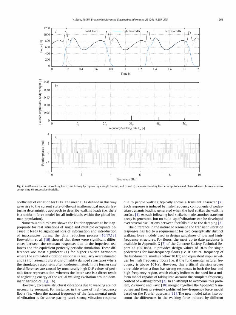
Measured continuous force time histories are invariably near-periodic (Fig. 1a), indicating their narrow-band nature (Fig. 1band c). However, to simplify analysis and utilisation of the mea-sured forcing time histories in design, they have usually been as-sumed to be perfectly periodic. This means that actual forces dueto continuous walking can be re-created or synthesised, by addinga sequence of identical single footfall traces, temporally displacedby integer multiples of an exact footfall interval (Fig. 2). Based onthis assumption, walking force time histories are presentable viaFourier series sinusoids:

F tð Þ ¼ a0 þXm

n¼1

an sin 2ptnfw þunð Þ ð1Þ

Here, F(t) is the synthetic forcing function, fw is pacing rate, a0 is amean value (equivalent to body weight of a pedestrian), an are har-monic amplitudes and un are the corresponding phase angles. Thevalue of m determines the number of harmonics considered in amodel. The simplest such model involving a single sinusoidal func-tion can be found in the current UK [3] and Canadian [4] designcodes for footbridges, while vibration design guidelines primarilyfor floors [5–8] provide for up to four harmonics. Some models evenuse up to the sixth harmonic [9]. In a time domain analysis proce-dure that uses such synthetic walking time series, the structure isassumed to be linearly elastic and, using modal decomposition,the response of each vibration mode can be analysed separatelyusing harmonic loads modulated by the appropriate mode shapeto account for the moving load [10].

http://dx.doi.org/10.1016/j.aei.2010.07.004

mailto:[email protected]



http://dx.doi.org/10.1016/j.aei.2010.07.004

http://www.sciencedirect.com/science/journal/14740346

http://www.elsevier.com/locate/aei

Nomenclature

Ti cycle intervalssi normalised cycle intervalsSs(f) ASD of si

As Fourier amplitudes of si

Wj, Aj Gaussian heights (weights)cj, tj, hj Gaussian centres

bj, dj, bj Gaussian widthsIw,i weight normalised impulsesDIw,i disturbance termq0, q1 coefficients of linear regressionxi angular frequency of rotationZk(t) shapes of successive cycles

260 V. Racic, J.M.W. Brownjohn / Advanced Engineering Informatics 25 (2011) 259–275

Phase angles have been found to vary considerably betweenvarious measurements [11,12], indicating that their random natureshould be considered when generating synthetic walking loads.However, little utilization of this important finding has been madeto date. The values of normalised coefficients an = an/a0 are oftenreported as dynamic load factors (DLFs) and depend on walkingspeed and individual characteristics of a human test subject [1].

]N[

sedutilpma

ecroF

T

86420

total force right1200

1000

800

600

400

200

0

0.25

0.15

- 4

w/ycneuqerF

0

0.20

0.10

0.05

0

]-[thgiew

ydob/seduti lpma

reiruoF

Frequ

4321 0

- 3

- 2

- 1

0

4

3

2

1

]dar[sesahp

re iruoF

0.5fw fw 1.5fw 2fw 2.5fw

a)

b)

c)

Fig. 1. (a) An example of continuously measured walking force signal and (b and c) the csuccessive footfalls.

The DLFs for walking, running, and jumping are presented by Rain-er et al. [13] for three subjects, while a more comprehensive studyof walking has been undertaken by Kerr [14]. His study found widevariability of DLFs among subjects participating in the tests (inter-subject variability) and also among different tests with the samesubject (intra-subject variability). Based on Kerr’s data, Young[15] described this variability by frequency-dependent mean and

20

ime [s]

1816141210

footfalls left footfalls

f ]-[etargnikla w

10

ency [Hz]

98765

3fw 3.5fw 4fw 4.5fw 5fw

orresponding Fourier amplitudes and phases derived from a window comprising 64

Time [s]

0.2 20

]N[

ecroF

1200

00.4 0.6 0.8 1 1.2 1.4 1.6 1.8

0.25

0.15

- 4

0.20

0.10

0.05

0

]-[thgiew

ydob/sedut ilpma

rei ruoF

10

Frequency [Hz]

86420

- 2

0

4

2

]dar[sesa hp

reiruoF

a)

b)

c)

1000

800

600

400

200

total force right footfalls left footfalls

Frequency/walking rate [-]fw

0 fw 2fw 3fw 4fw 5fw

Fig. 2. (a) Reconstruction of walking force time history by replicating a single footfall, and (b and c) the corresponding Fourier amplitudes and phases derived from a windowcomprising 64 successive footfalls.

V. Racic, J.M.W. Brownjohn / Advanced Engineering Informatics 25 (2011) 259–275 261

coefficient of variation for DLFs. The mean DLFs defined in this waygave rise to the current state-of-the-art mathematical models fea-turing deterministic approach to describe walking loads (i.e. thereis a uniform force model for all individuals within the global hu-man population).

Numerous studies have shown the Fourier approach to be inap-propriate for real situations of single and multiple occupants be-cause it leads to significant loss of information and introductionof inaccuracies during the data reduction process [16,17,12].Brownjohn et al. [16] showed that there were significant differ-ences between the resonant responses due to the imperfect realforces and the equivalent perfectly periodic simulation. These dif-ferences are most significant (1) for higher Fourier harmonicswhere the simulated vibration response is regularly overestimatedand (2) for resonant vibrations of lightly damped structures wherethe simulated response is often underestimated. In the former casethe differences are caused by unnaturally high DLF values of peri-odic force representation, whereas the latter case is a direct resultof neglecting energy of the actual walking excitation around dom-inant harmonics (Fig. 1b).

However, excessive structural vibrations due to walking are notnecessarily resonant. For instance, in the case of high-frequencyfloors (i.e. when the natural frequency of the fundamental modeof vibration is far above pacing rate), strong vibration response

due to people walking typically shows a transient character [7].Such response is induced by high-frequency components of pedes-trian dynamic loading generated when the heel strikes the walkingsurface [1]. As each following heel strike is made, another transientdecay is generated, but no build-up of vibrations can be developedover several oscillations between footfalls due to the damping [2].

The difference in the nature of resonant and transient vibrationresponses has led to a requirement for two conceptually distinctwalking force models used in design guidelines of low and high-frequency structures. For floors, the most up to date guidance isavailable in Appendix G [7] of the Concrete Society Technical Re-port 43 (CSTR43). It provides design values of DLFs for singlepedestrians for low-frequency floors (i.e. if natural frequency ofthe fundamental mode is below 10 Hz) and equivalent impulse val-ues for high frequency floors (i.e. if the fundamental natural fre-quency is above 10 Hz). However, this artificial division provesunreliable when a floor has strong responses in both the low andhigh-frequency region, which clearly indicates the need for a uni-form model capable of taking into account the complete frequencycontent of walking forces [2]. In an attempt to overcome this prob-lem, Zivanovic and Pavic [18] merged together the Appendix G im-pulses and their previously published low-frequency force modelbased on the Fourier approach [11]. The new model takes into ac-count the differences in the walking force induced by different


people and, as a result, can estimate the probability distribution ofvibration responses generated by a pedestrian population. How-ever, Middleton showed recently that inter-subject variations donot affect the dynamic response as much as variations in an indi-vidual’s pace rate for successive steps [19]. In the case of high-fre-quency floors, a lack of these variations can overestimate responseup to 40%. A number of authors [20,16] showed that the actual nar-row-band effect seen for real loads was more suited to the tech-niques of stochastic analysis in frequency domain, where themeasured forces are presented as auto-spectral densities (ASDs).The resulting response prediction (typically acceleration) is neces-sarily given as a root mean square (RMS) value, and this is consis-tent with commonly used vibration acceptance criteria [7].However, this single number contains no information about ex-pected performance of the structure in real time while human ac-tions are taking place (e.g. where the peak responses are and howoften they happen, as it can be described by peak and crest factors).For such advanced analysis, a reliable time domain model of walk-ing forces is clearly the way forward.

The most comprehensive dataset on walking forcing functionsavailable worldwide currently is based on data from approximately1000 individual time series generated by about 40 individuals col-lected by Kerr [14] as they passed over a force plate and made asingle footfall. However, apart from the limited number of test sub-jects, the key problem with this data set is that it cannot representthe variability of real walking between subsequent steps of thesame pedestrian during one walking exercise. Gait, or ‘manner ofwalking’, is the subject of considerable research in the biomechan-ics community [1]. However, no database of walking forces in theform of continuously recorded time series has yet been found thatcan be used for development of statistically reliable characterisa-tion of these forces for application in a civil engineering context.

By combining multidisciplinary experimental and analytical ap-proaches, this paper advances the field by bringing together: (1) anextensive database of continuously measured vertical walkingforces generated by individuals, and (2) a unique stochastic modelof these forces which can simulate accurately what is being mea-sured. This includes modelling of near-periodic features of actualforces, such as variations in timing, shape and amplitudes, as wellas the complete frequency spectrum. An instrumented treadmillfor experimental identification of the forces was transferred andadapted from the biomechanical field of human locomotion [21],while the modelling strategy was motivated by existing modelsfor replicating human electrocardiogram (ECG) signals [22] andspeech recognition [23]. Therefore, the paper presents a new gen-eration of synthetic walking loads which is a radical departurefrom the conventional models used in the current design guide-lines for pedestrian structures and which, more importantly, cansimulate reality better.

2. Experimental data acquisition

A database comprising many high-quality walking force recordsis an essential component for the development of a stochasticmodel of individual walking loads. Section 2.1 aims to justify thechoice of equipment used in this study to build such a database.This is followed by a brief description of the experimental setupin Section 2.2 and details on test protocol in Section 2.3, so thatit is clear how the data was collected.

2.1. Instrumentation for measuring contact forces during continuouswalking

Dynamic forces generated by people walking on a structure areideally determined by direct measurement of the contact forces

between the feet and the structure itself, hence they are generallyknown as ground reaction forces (GRFs). For this purpose Raineret al. [13] used a continuously measured reaction of a floor striphaving known dynamic properties, whereas Ebrahimpour et al.[24] used a short length of walkway instrumented with severalforce plates. However, such an experimental setup can provideforce records for a limited number of successive footfalls and re-quires considerable laboratory space. One solution to overcomethese drawbacks is to use an instrumented force measuring tread-mill (IFMT). It requires less laboratory space and enables quick col-lection of GRFs during a large number of successive cycles and overa wide range of steady-state gait speeds [25]. Although there is notheoretical difference in the physics of treadmill and overgroundlocomotion, some early experimental studies based on very rudi-mentary treadmill designs reported significant discrepancies be-tween overground and by treadmill measured GRFs [26], as wellas with temporal and spatial parameters of gait such as step lengthand step frequency [27]. The reason for this was thought to be im-posed ‘constant’ speed of movement, controlled by rotation of thetreadmill belt, as opposed to the overground locomotion when thegait speed has no similar control [28]. More recently, using theiradvanced treadmill design [29,30] performed a series of experi-ments to make more accurate comparisons between treadmill ver-sus overground walking. Although it was possible to detect subtledifferences in kinematics and kinetics of human gait, the magni-tudes of these differences were within a normal range of variabilityof the gait parameters in the biomedical domain. Interestingly, vande Putte et al. [31] reported that differences between treadmill andoverground walking vanished after only ten minutes of practice oftreadmill walking in the case of inexperienced treadmill users. Thiswas concluded based on comparison between three-dimensionalknee kinematics and step lengths recorded on ten healthy test sub-jects as they walked on a treadmill and ‘free-field’. These studiesdemonstrated the essential equivalence of treadmill and over-ground gait in biomedical application, such as design of prostheticlegs and artificial hip joints. Hence, they justified treadmill-basedforce measurements used in this paper for design of less delicatecivil engineering structures.

2.2. Experimental setup

All walking tests were carried out in the Light Structures Labo-ratory in the University of Sheffield. Continuously measured forcerecords were collected of one person walking at a time on thestate-of-the-art instrumented treadmill ADAL3D-F [32]. The tread-mill is installed in a recessed pit and flush with the laboratory floor,as illustrated in Fig. 3.

To measure independently the left and right footfalls, ADAL3D-Fdesign includes two identical IFMTs, one for the left and one for theright side of the walking area (Fig. 3). All components (including amotor, belt and secondary elements) of each treadmill are mountedon a single metal frame and mechanically connected to the support-ing ground only through a pair of Kistler 9077B three-axial piezo-electric force sensors [33]. Therefore, assuming the rigidity of theabove mentioned ensemble, the entire treadmill is mechanicallyisolated. This means that the forces due to belt friction and belt rota-tion can be considered as internal forces and are not detected by thesensors [21]. The stiffness constants for the force sensors are largeenough that natural frequencies of the supported treadmill frameare very high compared to the bandwidth of significant walkingforces. Thus, the sensors measure only external forces, i.e. actualthree-axial forces exerted by the feet on the treadmill belts. Onlythe vertical time series are considered here (Fig. 1a), while lateraland longitudinal components are beyond the scope of this paper.

Each treadmill belt is driven by a brushless servomotorequipped with internal velocity controllers to maintain the speed

Fig. 3. Experimental setup.


as constant as possible. Velocity of treadmill belts in the range 0.1–10 km/h can be controlled and monitored remotely either with acontrol panel or with ADAL3D-F software, Adisoft2000 [32], runfrom the data acquisition PC. Similar to fitness treadmills, the re-mote control panel and the treadmill itself are equipped with asafety stop switch.

2.3. Test protocol

Prior to the measurements, a test protocol approved by the Re-search Ethics Committee of the University of Sheffield requiredeach participant complete a Physical Activity Readiness Question-naire and pass a preliminary fitness test (by satisfying predefinedcriteria for blood pressure and resting heart rate) to check whetherthey were suited for physical activity required during the measure-ments. Also, measurements of the body mass, age and height weretaken for each test subject who passed the preliminary test. Allparticipants wore comfortable flat sole shoes.

Participants who had no experience with treadmill walkingwere given a brief training prior to the measurements supervisedby a qualified instructor. All test subjects did approximately ten

total force right

Ti

0

]-[thgiew

ydob/ ecroF

1.6

1

00.5 1

area = Iw,i

Ti

1.4

1.2

0.8

0.6

0.4

0.2

footfall

Fig. 4. A portion of a continuously measured GRF due

minutes long warming up, which included walking on the tread-mill while the walking speed was varied randomly and controlledby the speed of rotation of the treadmill belts. As already explainedin the previous section, this interval was reported as long enoughfor pre-test habituation to treadmill walking, when differences be-tween treadmill and overground walking vanish even for inexperi-enced test subjects [31].

The acquisition of walking forces started at a speed of 2 km/hand continued in increments of 0.5 km/h up to the maximum com-fortable walking speed, which was determined by each test subjectindividually. This speed differs between people and depends pri-marily on the length of a test subject’s legs and therefore theiroverall height [34]. Pacing rate was not prompted by any stimulisuch as a metronome, and it was determined only from subsequentanalysis of the generated force signals.

Each test followed the same pattern whereby a participant wasfirst asked to stand still on the treadmill, and then:

(1) was informed when the treadmill belts would start rotatingat a particular constant speed,

(2) was asked to walk until at least 64 successive footfalls wererecorded,

(3) was informed when the treadmill will be stopped,(4) was asked to keep walking until the treadmill came to a halt,

and(5) was asked to leave the treadmill and rest.

In total, 80 volunteers (55 males and 25 females, body mass76.1 ± 15.3 kg, height 174.8 ± 8.1 cm, age 29.7 ± 9.3 years) weredrawn from students, academics and technical staff of the Univer-sity of Sheffield. On average, forces corresponding to ten differentwalking speeds were collected for each test subject depending ontheir maximum comfortable walking speed. All together they gen-erated 824 vertical walking force time series of kind illustrated inFig. 1a. Each walking time series was sampled at 200 Hz.

3. Modelling individual force signals

This section describes the concept of the new model develop-ment, from analysis of continuous walking parameters of a singleforce record to its synthetic counterpart, so the reader can followthe rationale for the remaining parts of the paper. In Section 4 itwill be applied to each force record in the database presented inSection 2 yielding a mathematical generator of stochastic near-periodic walking time series.

footfalls left footfalls

me [s]

31.5 2 2.5

Ti+1

walking cycle = stride

to walking. The total duration of the signal is 40 s.


3.1. Basic processing of measured force records

Fig. 4 illustrates a portion of a continuously measured forcetime history generated by a single person walking at 5 km/h and1.81 Hz pacing rate. The force signal was filtered using a fourth-or-der low-pass Butterworth digital filter having cut-off frequency at60 Hz.

It is apparent that there is some variation in shape of footfallforces (i.e. pulses), intervals and force amplitudes on a step-by-stepbasis. IFMTs are normally used in biomechanics of human gait toprovide a series of statistics or gait parameters describing footfalls[1]. However, data relevant for structural analysis concerning in-tra-subject variations in timing of the individual footfalls and theiramplitudes are not readily available from the literature.

Closer inspection also reveals differences between the left andright footfalls. For instance, the left footfalls have greater first peakof the characteristic ‘M’ shape. Sahnaci and Kasperski [35] showedthat this asymmetry in walking induces intermediate harmonicload amplitudes (so called ‘sub-harmonics’ which are illustratedin Fig. 1b) which may lead to larger vibration responses than high-er integer harmonics for some test subjects. Therefore, in this studythe total vertical force will be modelled on a stride-by-stride basis,where a stride (i.e. walking cycle) consists of two successive foot-falls, left and right (Fig. 4).

A walking cycle can be defined between any two nominallyidentical events of the total force signal. Since the amplitudes ofthe total vertical forces oscillate around body weight of the testsubject, the point close to the beginning of the left footfall whereamplitude of the total force is equal to body weight was selectedas starting (and completing) event (Fig. 4). From the 40 s long forcesignal illustrated in Fig. 4 yielding about 72 footfalls, a windowcomprising 32 successive cycles (64 footfalls) was extracted fromthe middle of the signal for further analysis.

Fig. 5 shows values of normalised impulses Iw,i as a function ofthe cycle intervals Ti. The normalised impulse is defined as the cy-cle impulse (i.e. the integral of the force over Ti) divided by testsubject body weight. The apparent linear trend between thesetwo parameters offers an opportunity to describe weight norma-lised impulses as a function of the cycle intervals. However, bear-ing in mind the definition of a cycle impulse, the linear trenddoes not indicate that the peak force amplitudes of successive cy-cles depend on the corresponding cycle intervals. This is an impor-tant feature for the proposed methodology, as will be shown laterin Section 3.5.

Cycle intervals T [s]i

1.161.151.07 1.08 1.09 1.10 1.11 1.12 1.13 1.141.07

1.08

1.09

1.10

1.11

1.12

1.13

1.14

1.15

1.16

Iseslup

midesila

mroN

[-]

i,w

measured data

linear fit

Fig. 5. Linear trend between periods Ti and weight normalised impulses Iw,i.

3.2. Variability of cycle intervals

Variations of intervals Ti (i = 1, . . . ,32) can be represented by asequence of dimensionless numbers calculated as:

si ¼Ti � lT

lT

lT ¼mean Tið Þð2Þ

Three methods were tried for modelling si data. Histogram of si

amplitudes (Fig. 6) indicated that this data set does not follow anyknown probability distribution. Small number of data points couldbe argued, but the same was found for the variations of twice asmuch footfall intervals. Next, it was assumed that the current si va-lue is a linear combination of previous k values si�1, . . . ,si�k, whichcould be described by an autoregressive model [36]. This methodproved unreliable since weak correlation was found between theprevious and subsequent si values for increasing order of regres-sion from one to five (k = 1, . . . ,5). Finally, utilisation of the auto-spectral density (ASD) of a random process resulted in a success.

The variance r2x of a real random process x(t) can be obtained as

the total area under its ASD Sx(f) as [37]:

r2x ¼

Z 1

0Sx fð Þdf ð3Þ

Hence, the aim is to use ASD of actual si series to generate syn-thetic s0i series with the same statistical properties, such as stan-dard deviation and ‘structure’ of variation between successive si

values. Under assumption that the variation of si does not changefor the given test subject, pacing rate and duration of walking(e.g. caused by fatigue and physical discomfort), this appliesregardless of the number of discrete data points in the measuredand artificial data sets, which will be demonstrated later in thissection.

The ASD of si can be calculated as:

Ss fmð Þ ¼A2

s fmð Þ2Df

; f m ¼m32

; m ¼ 0; . . . ;15 ð4Þ

where A2sðfmÞ is a single-sided discrete Fourier amplitude spectra

having spectral line spacing Df ¼ 1=32 (Fig. 7).The ASD ordinates do not depend on the number of discrete

data points si used for the calculation of As(fm) via Fast FourierTransform (FFT) but it is coarse due to the limited number of points

0

]-[secnarucco

foreb

muN

-0.0

36

-0.0

22 510.0-

0

0.01

5

0.02

2 920.0

630.0

1

2

3

7

6

5

4

Normalised cycles intervals i

040.0

040.0-

Fig. 6. Histogram of si values.

Cycles [-]

30252015105 231

1.15

1.14

1.13

1.12

1.11

1.10

1.09

1.08

1.07

]s[T

slavretnielcy

Ci

syntheticmeasured

Fig. 8. Measured si and an example of synthetic s0i series.


(16 single-sided FFT). More points might reveal a much richerstructure but this requires a longer walking force signal. However,concerning ethics in research, the duration was limited to avoid fa-tigue and discomfort, which can also influence natural variabilityof the force records.

The ASD Ss(fm) can be analytically represented by a series ofGaussian functions (Fig. 7):

S0s fð Þ ¼X16

j¼1

Wje�

f�cjð Þ22b2

j ð5Þ

here, parameter Wj is the height of the jth Gaussian peak, cj is theposition of the centre of the peak, and bj controls the width (i.e. timeduration) of the corresponding Gaussian function. The Gaussiancentres cj, j = 1, . . . ,16, are placed in each sample on the quasi-fre-quency axis in order to fit exactly the measured ASD (Fig. 7). Forsuch fixed positions of cj and predefined widths bj = Df, Gaussianheights Wj (also called weights) can be computed using the non-lin-ear least-square method [38].

Representation of the discrete ASD Ss(fm) in the form of the con-tinuous function S0sðf Þ enables generation of synthetic seriess0iði ¼ 1; . . . ;NÞ of arbitrary length (e.g. N� 32), which will havestatistically the same properties of variations on the sample-by-sample basis as the measured set of 32 actual si data points. Thisis done by calculating a new set of ASD amplitudes for a sequenceof discretely spaced frequency points fn = nDf0 using Eq. (5), wheren = 0, . . . ,N/2 � 1 and Df0 = 1/N. The new set of ASD amplitudesS0sðfnÞ and Eq. (4) are then used to generate a new set of Fourier

amplitudes A0sðfnÞ ¼ffiffiffiffiffiffiffiffiffiffiffiffiffiffiffiffiffiffiffiffiffi2Df 0S0sðfnÞ

q. Finally, assuming random distri-

bution of phase angles in the range [�p,p], these amplitudes areused in inverse FFT algorithm to generate a synthetic set of N vari-ations s0i. Different realisations of the random phases may be spec-ified by varying the seed of the random number generator, hencemany different series s0i may be generated with the same spectralproperties (Fig. 8).

According to Eq. (2), scaling s0i by lT and adding the offset valuelT calculated from the measured Ti data, results in a series of syn-thetic intervals T 0i, as would be generated by the test subject duringnominally identical walking exercises. Empirical evidence for thisis presented in Section 3.5.

0.10 0.2 0.3 0.4 0.5

c1 c4 c8 c12 c16

12

10

8

6

4

2

0

Quasi-frequency [-]

foDS

Ai[

-]

measured

fit

x 10-4

Fig. 7. Single-sided ASD of si values.

3.3. Variability of normalised impulses

The measured weight normalised impulses Iw,i can be expressedas a function of the cycle intervals Ti (Fig. 9) using the following lin-ear regression model [39]:

Iw;i ¼ q1Ti þ q0 þ DIw;i ð6Þ

Here, q1 = 1.05 and q0 = � 0.05 are regression coefficients andDIw,i is the subsequent error (also known as a disturbance term),which is a random variable. Given the regression coefficients q1

and q0, DIw,i, can be calculated as:

DIw;i ¼ Iw;i � q1Ti � q0 ð7Þ

It is common to model DIw,i as a random noise having a Gauss-ian distribution [39].

Given a set of synthetic cycle intervals T 0i generated as explainedin Section 3.2, a series of the corresponding synthetic normalisedimpulses I0w;i can be calculated using Eq. (6). These are used in Sec-tion 3.5 to scale amplitudes of successive strides, thus make asmooth transition of walking energy between successive cycles.

Tme [s]

1.210.80.60.40.20-0.4

-0.3

-0.2

-0.1

0

0.1

0.2

0.3

0.4

0.5

]-[ecrof

desilamro

N

Fig. 9. Normalised walking cycles.

Tme [s]

1.210.80.60.40.20-0.4

-0.3

-0.2

-0.1

0

0.1

0.2

0.3

0.4

]-[ecrof

desilamro

N

Gaussianstemplate fit

Fig. 11. Fitting the template cycle with a series of Gaussian basis functions.


3.4. Template waveform of walking force signals

The 32 normalised walking cycles have been detrended (bodyweight has been removed), resampled to the maximum length ofall the cycles and aligned with respect to the common time axis,as shown in Fig. 9. Visual inspection suggests that there is a com-mon waveform of the walking force which distorts along time andamplitude axes on a cycle-by-cycle basis. The key challenge here isto extract this waveform and provide its reliable mathematical rep-resentation which can be used to generate synthetic time series.

The average cycle is considered unreliable representative due tomisalignments and shifts of the common events, such as positionsof the local extreme values. To correct for these slight variations, aprocedure called dynamic time warping (DTW) is applied to themeasured cycles before their average is calculated. DTW was orig-inally developed for speech recognition [23], but in recent years ithas found application in a fingerprint verification [40], chromatog-raphy [41] and in gene expression studies [42]. The procedure non-linearly warps the two trajectories in such a way that similarevents are aligned and the summed squared differences are mini-mised [23]. This process is illustrated schematically in Fig. 10a.Similarly, wavelet analysis linearly shifts and stretches the original(or mother) wavelet. However, due to the apparent nonlinear mis-alignments of the common events in the force data, linear shiftingand stretching is unsuitable for determining the template cycle.

Since the DTW method warps two cycles at one time, the nexttask is to choose the reference cycle and then warp all the other cy-cles onto that one. Such a cycle minimises the sum of Euclidieandistances between each data point to the average of all the cycles[43]. When the warping has been completed and the commonevents in the cycles aligned, the template cycle is formed as aver-age of the warped cycles, as illustrated in Fig. 10b.

For fs = 200 Hz sampling rate and interval of 1.15 s, the underly-ing shape of the template cycle (Fig. 10b) can be modelled mathe-matically as a sum of 115 Gaussian functions Z(t):

Z tð Þ ¼X115

j

Aje�

t�tjð Þ22d2

j ð8Þ

where the parameter Aj is the height of the jth Gaussian peak, tj isthe position of the centre of the peak, and dj is the width of the cor-responding Gaussian functions in the sum (Fig. 11).

The Gaussian centres tj = nDt (n = 1, . . . ,115, Dt = 2/fs) areplaced in every second sample on the time axis to fit accurately

Tme [s]

1.210.80.60.40.20-0.4

-0.3

-0.2

-0.1

0

0.1

0.2

0.3

0.4

0.5

]-[ecrof

desilamro

N

reference trajectory warping trajectorya)

Fig. 10. (a) Schematic illustration of dynam

the normalised force amplitudes, thus to reflect completely thecorresponding Fourier amplitude spectrum. A less dense distribu-tion of Gaussian functions (e.g. centres are placed in every thirdor fourth sample) makes the fit smoother causing the high-fre-quency components to vanish. For such fixed positions of Gaussiancentres and predefined widths dj = 2Dt, Gaussian heights Aj can beoptimised using non-linear least-square curve fit [38].

Scaled in the vertical and horizontal direction, analytical func-tions Z(t) can be used to generate artificial force signals which re-flect the variations of impulses and intervals for successive walkingcycles. This is demonstrated in the next section.

3.5. Dynamic model

A repetitive walking pattern could be better visualised whenthe template cycle is ‘wrapped’ around the surface of a circular cyl-inder (Fig. 12). Now the first and the last sample of the templateoverlap, thus the corresponding trajectory becomes a closed orbitin three-dimensional (3D) space with coordinates (r, h, z). A syn-thetic time series is generated by retracing the fit Z(t) around thecircle of unit radius in (r, h) the plane (Fig. 12). Each revolutionon this circle corresponds to one interval of walking cycle.

The equations to generate synthetic forces are therefore givenby a set of three coupled equations:

Tme [s]

1.210.80.60.40.20-0.4

-0.3

-0.2

-0.1

0

0.1

0.2

0.3

0.4

0.5

]-[ecrof

desilamro

N

template warped signalsb)

ic time warping. (b) Template cycle.

z

rj

Fig. 12. Trajectory of the template cycle in a three-dimensional (3D) space.


r tð Þ ¼ 1h tð Þ ¼ xt

Z hð Þ ¼X115

j

Aje�

h�hjð Þ22b2

j

ð9Þ

where x is angular frequency of rotation and bj = xdj in rads. Thetime positions of the Gaussian centres tj in Eq. (8) now correspondto fixed angles hj = xtj around the unit circle, as illustrated inFig. 12.

Variations in the length of successive intervals can be incorpo-rated by varying angular frequency of rotation x. Its values for suc-cessive revolutions can be calculated as:

x0i ¼2pT 0i

ð10Þ

where T 0i ði ¼ 1; . . . ;NÞ are synthetic intervals of walking cyclesgenerated as explained in Section 3.2. Moreover, having T 0i series,values of the corresponding synthetic normalised impulses I0w;i canbe calculated by using Eq. (6). These are assigned to the synthetictime series generated by Eq. (9) by multiplying amplitudes of suc-cessive cycles by appropriate scaling constants and adding an offset

Tim

15100 5

1.5

0.6

1.3

1.1

0.90.8

1.4

1.2

1

0.7

]-[thgie

wydob

/ecroF

1.5

0.6

1.3

1.1

0.90.8

1.4

1.2

1

0.7

]-[thgie

wydob

/e croF

a)

b)

Fig. 13. (a) Measured and (b) an example of synthetic wa

of unit amplitude to each data point. The resulting signal is an arti-ficial, weight normalised walking force time series.

Measured continuous walking series and an example of its syn-thetic counterpart are shown in Fig. 13a and b, respectively. Visualcomparison suggests that the uniform scaling of the template cycleis not the way to model inter-cycle variations of the walking forceamplitudes.

However, no model has been found to describe variations of theGaussian heights Aj as a function of variations in the cycle intervals.Existence of such a model was already questioned in Section 3.3due to the strong linear correlation between the cycle intervalsand the normalised impulses (Fig. 5).

Fig. 14 shows the discrete Fourier amplitude spectra of the mea-sured and synthetic signals. To avoid leakage during the digital sig-nal analysis, the duration of data blocks used to calculate thespectra was fixed at exactly 32 cycles. While the dominant har-monics (i.e. integer multiples of the pacing rate fw = 1.81 Hz) aremodelled reliably, there is less ‘spread’ of energy to adjacent spec-tral lines of synthetic data through lack of inter-cycle variability offorce amplitudes. The effect is more prominent for higher harmon-ics, which can be illustrated better by comparing quasi steady-state structural responses of a single degree of freedom (SDOF)oscillator after the initial transient build up.

3.6. Quantification of structural response and model validation

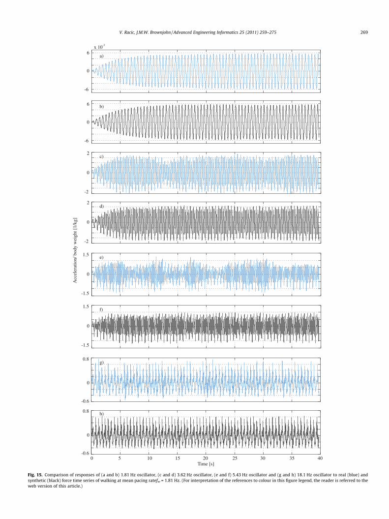
The blue line in Fig. 15 shows response to the measured walkingtime series for a 1000 kg oscillator with 2% damping and naturalfrequencies of 1.81, 3.62, 5.43, and 18.1 Hz. These frequencies f cor-respond exactly to the fundamental and higher harmonics of thewalking excitation. The response of the same oscillators to the syn-thetic excitation (black lines) is given below the response to realwalking for comparison.

Visually, there is no significant difference between the two re-sponses when the natural frequency of the oscillator exactly equalsthe mean pacing rate (f = fw). The comparison also demonstratesthat it is possible to build-up to a significant percentage of reso-nant response to the fundamental component of the walking forceeven with real, more variable walking.

For the second and third harmonics, the difference is muchclearer, particularly for the third harmonic. On average, the SDOF

e [s]

302520 35 40

lking time series generated using the template cycle.

12108640 14 16 18

Frequency [Hz]

0.25

0.20

0.15

0.10

0.05

0

0.25

0.20

0.15

0.10

0.05

0

/sedutilpma

reiruoF]-[thgie

wydob

/sedu tilpma

reiru oF]-[th gie

wydob

a)

b)

2

Fig. 14. Discrete Fourier amplitudes of (a) measured and (b) synthetic walking time series. Figs. 13 and 14 represent the same data.


systems have greater response under the excitation of a syntheticwalking. However, occasionally the response due to real excitationexceeds its less variable synthetic counterpart. Also note that afterthe transient build up to a significant proportion of resonant max-imum amplitude, the response fades. A number of authors [44,17]observed this phenomenon with pedestrians exciting very livelyfootbridges in anti-symmetric vertical modes. When the pacingof a pedestrian becomes out of phase with the vibration of a foot-bridge structure excited close to resonance, energy is extractedfrom the structure and the human exciter becomes an active dam-per. More recently, the authors offered more formal proof of thishappening by studying energy flow between active humans anda lively structure due to bouncing and jumping [1].

Similarly to the first harmonic, there is little to choose betweenthe two responses when the natural frequency of the oscillator isten times higher than the mean pacing rate (f = 10fw). However,it is worth noticing that occasionally the real response exceeds itsynthetic counterpart. Peak vibration amplitude is a commonlyused vibration acceptance criteria for floors accommodating sensi-tive equipment, such as lasers in operating theatres [2].

Further parametric studies can demonstrate that the differencesreduce with increase of damping of the SDOF systems studied butare still significant even for damping as high as 3% found in modernoffice floors with full-height partitions. To get more reliable predic-tion of vibration response, a logical way forward is development ofa more comprehensive model of inter-cycle variations of the forceamplitudes which will account for non-uniform scaling. Such amodel is presented in the next section.

3.7. Variability of amplitudes of walking cycles

Each of the 32 signals shown in Fig. 9 is fitted to Eq. (8) yieldingindependent analytical functions Zk(t), k = 1, . . . ,32. Under assump-tion that the variations of cycle intervals and morphology of thecorresponding force signals do not correlate, the Zk(t) shapes canbe assigned in a random order to synthetic walking cycles. Evenwhen the same Zk(t) is assigned to different cycles, the resultingsignal generated by the coupled system of Eq. (9) will be slightlydifferent. This is because there are two more random parametersx0i, and I0w;i, which influence morphology of the signals. Higher

angular frequencies x0i generate the cycles faster, hence they com-press them and vice versa. As shown in Section 3.5, by multiplyingamplitudes of each cycle by appropriate scaling constants and add-ing the offset value, the resulting time series are assigned the cor-responding I0w;i values.

The similarity between the real measured and synthetic walk-ing forces is illustrated by comparison of Fig. 16a and b. Also, thestandard Fourier amplitude spectra are compared in Fig. 17, whilevibration responses for the SDOF systems defined in the previoussection are shown in Fig. 18. This comparison looks much betterthan in Sections 3.5 and 3.6 between actual and uniformly scaledamplitudes of synthetic forces.

Perfectly identical synthetic signals can be generated only bychance due to the omnipresent randomness of the modellingparameters. However, a family of synthetic forces share severalproperties inherited from their common measured counterpart:

(1) Shapes of the walking cycles are drawn from the samesource (i.e. Zk(t) functions), where each shape has the sameprobability of occurrence.

(2) Variations of successive cycle intervals T 0i are the same for allsynthetic signals because they have the same ASD.

(3) The statistical equivalence between T 0i values reflectsdirectly equivalence between the corresponding weight nor-malised impulses I0w;i according to Eq. (6). This implies thattotal energies of generated signals are statistically the same.

4. Development of stochastic walking model

This section integrates everything presented so far to create anumerical generator of stochastic near-periodic walking force sig-nals. Section 4.1 deals with organisation of the modelling parame-ters extracted (as explained in Section 3) from the numerousdatabase of the individual force records collected in Section 2. Thisis followed by a description of the mechanism underlying genera-tion of random walking loads in Section 4.2.

4.1. Utilisation of existing database

The 824 force signals measured in Section 2 were classified into20 categories (clusters) with respect to the actual pacing rate, as

-6

0

6x 10

-3

-6

0

6

-2

0

2

-2

0

2

-1.5

0

1.5

-1.5

0

1.5

-0.6

0

0.8

-0.6

0

0.8

0 5 10 15 20 25 30 35 40Time [s]

b)

a)

c)

d)

e)

f)

g)

h)

]gk/1[thgiew

ydob/noitareleccA

Fig. 15. Comparison of responses of (a and b) 1.81 Hz oscillator, (c and d) 3.62 Hz oscillator, (e and f) 5.43 Hz oscillator and (g and h) 18.1 Hz oscillator to real (blue) andsynthetic (black) force time series of walking at mean pacing ratefw = 1.81 Hz. (For interpretation of the references to colour in this figure legend, the reader is referred to theweb version of this article.)


Time [s]

30252015100 355 40

1.5

0.6

1.3

1.1

0.90.8

1.4

1.2

1

0.7

]-[thgie

wydob

/ecroF

1.5

0.6

1.3

1.1

0.90.8

1.4

1.2

1

0.7

]-[thgie

wydob

/e croF

a)

b)

Fig. 16. (a) Measured and (b) synthetic walking time series which accounts for inter-cycle variations of force amplitudes.

12108640 142 16 18

Frequency [Hz]

0.25

0.20

0.15

0.10

0.05

0

0.25

0.20

0.15

0.10

0.05

0

/sedutilpma

reiruoF]-[thgie

wydob

/sedutilpma

reiruo F]-[ thgie

wydob

a)

b)

Fig. 17. Discrete Fourier amplitude spectra of the signals shown in Fig. 16.


shown in the histogram in Fig. 19. Each bar in the histogram isapproximately 0.1 Hz wide. For example, all force records withthe pacing rate in the range 1.58–1.68 Hz are gathered into onecluster. Such fine resolution is a key feature for development of astochastic model outlined in the next section.

Note that walking at different speeds does not necessarily yielddifferent pacing rates. This is because people unconsciously controltheir step length to walk at their most comfortable pacing rate[45]. In the present study, the cluster for the rates between 1.88and 1.98 Hz is the most numerous comprising 101 different walk-ing force records. This might be an indicator that this is the rangeof the most comfortable pacing rates for the majority of partici-pants in this study.

Each force history within a cluster was processed using the con-cept described in Section 3. Multiple sets of information (parame-ters of the Gaussian fits Zk(t) for and the ASD S0sðf Þ, autoregressioncoefficients q1 and q0 and the parameters of the Gaussian randomnoise) were extracted and stored within the cluster as MATLABstructure files [46]. This is an important aspect of the stochastic ap-proach adapted in this paper, as it will be demonstrated in the nextsection.

The key challenge now is to show that the force amplitudes areindependent of body weight, so that weight normalised syntheticforces of kind shown in Figs. 13b and 16b can be scaled by theweight of any person drawn by chance from the world’s popula-tion. By doing this, randomisation of the modelling parameters will

x 10-3

-6

0

6

-2

0

2

-1.5

0

1.5

-0.6

0

0.8

0 5 10 15 20 25 30 35 40

Time [s]

a)

b)

c)

d)

]gk/1[thgiew

ydo b/ noitareleccA

Fig. 18. Dynamic responses of (a) 1.81 Hz oscillator, (b) 3.62 Hz oscillator, (c) 5.43 Hz oscillator and (d) 18.1 Hz oscillator to synthetic force time series shown in Fig. 16b(mean pacing rate is fw = 1.81 Hz).

21.51

Pacing rate [Hz]

2.5 3

110

100

90

80

70

60

50

40

30

20

10

0

]-[secnerrucco

foreb

muN

Fig. 19. Histogram of pacing rates yielding 20 clusters.


be extended to the maximum. The evidence to support thishypothesis is given in Fig. 20, where DLF of the fundamental har-monic is plotted versus the corresponding body weight for all sig-nals in clusters 1.48–1.58 Hz, 1.88–1.98 Hz and 2.28–2.38 Hz.These clusters are selected as representatives of slow, moderate

and fast pacing rates. The scattered patterns for all three clustersindicate no correlation between the two parameters, thus theycan be treated as independent variables. Furthermore, body weightcan be modelled as a random parameter using a probability densityfunction, as suggested by Hermanussen et al. [47] for German, Aus-trian and Norwegian citizens.

4.2. Procedure for generating synthetic forces

The stochastic approach adopted in this paper rests on theassumption that a set of the modelling parameters selected ran-domly and equally likely from a cluster can be used to synthesisewalking time series at any pacing rate which falls within the clus-ter’s narrow frequency range. This means that the modellingparameters extracted from real walking at particular rate can beused to generate synthetic walking forces at rates which are closeenough.

The flow chart in Fig. 21 illustrates the complete process (algo-rithm) of creating synthetic GRF signals. For a specified pacing rateand duration of walking, the algorithm first estimates the totalnumber of walking cycles N. Then, from a frequency cluster corre-sponding to the pacing rate, it selects by chance a set of multiplemodelling parameters. At this point, the algorithm splits into twoactions. First, it creates intervals T 0i using the ASD S0sðf Þ (Section 3.2)and then calculates normalised impulses I0w;i using the regressive

Body weight [N]

1300120011001000900800700600500400

0.14

0.12

0.10

0.08

0.06

0.04

0.02

Body weight [N]

1300120011001000900800700600500400

0.40

0.35

0.30

0.25

0.20

0.15

0.05

0.10

0.55

0.50

0.45

0.40

0.35

0.30

0.15

0.20

0.10

0.05

Body weight [N]

700650600550500 059009058008057054

a) )c)b

]-[F

LD

Fig. 20. DLFs versus body weight for pacing rates in the range (a) 1.48–1.58 Hz, (b) 1.88–1.98 Hz and (c) 2.28–2.38 Hz.

from the corresponding cluster select aset of the force parameters by chance

input data: pacing rateand duration of walking

number of cycles N

random number seed phases [- ]

random number seed

generation of syntheticwalking cycles Ti

coupled system of equations

weight normalised GRFs

random number seed

pdf of body weight

body weight

synthetic GRF signal

ASD of variations ofcycle intervals S (f)

weight normalised impulses Iw,i

generation of the correspondingangular frequencies i

shapes Z (t)k

Fig. 21. Algorithm for generating synthetic time series.


model given by Eq. (6). The algorithm then assigns randomly andequally likely one of the functions Zk(t) to each of the N walkingcycles.

The next step integrates everything generated so far to run thedynamic model (Section 3.5) and therefore to generate weight nor-malised walking forces of a kind shown in Fig. 16b. Finally, thesebecome equivalent walking force time histories when their ampli-tudes are additionally multiplied by random body weight.

Fig. 22 shows examples of the signals generated when the mod-el is run twice in succession for the pacing rate 2 Hz lasting 30 s. Avisual comparison of the two signals provides convincing evidencethat the model can account for the inter-subject variability in theshapes and force amplitudes. On the other hand, the ability ofthe model to generate different degrees of intra-subject variabilityfor different persons becomes more obvious from comparison be-tween the corresponding frequency spectra (Fig. 23). The broader

spread of energy around dominant harmonics (i.e. integer multi-ples of 2 Hz) and existence of sub-harmonics (i.e. integer multiplesof 1 Hz) in Fig. 23a relative to b indicates that the first ‘virtual’ pe-destrian varies their walking more.

5. Conclusions

A data-driven mathematical concept has been developed formodelling dynamic loads generated by pedestrians walking. Theability to replicate temporal and spectral features of real walkingloads, and therefore simulate reliably dynamic response of struc-tures carrying pedestrians, gives this model a definite advantageover the existing walking models which can be found in the cur-rent UK and worldwide design guidelines for pedestrian structures,such as footbridges and floors. Therefore, the model presented in

Time [s]

30252015100 5

1400

]N[

ecroF

1200

1000

800

600

400

1100

]N[

ecroF

1000

800

600

400

900

700

500

300

a)

b)

Fig. 22. Examples of synthetic time series for walking rate 2 Hz and duration 30 s.

12108640 142

Frequency [Hz]

0.25

0.20

0.15

0.10

0.05

0

/sedutilpma

reir uoF]-[ thgi e

wy dob

0.25

0.20

0.15

0.10

0.05

0

/sedutilpma

reiruoF]-[thgie

wydob

0.30

0.35a)

b)

Fig. 23. Discrete Fourier amplitudes of the signals shown in Fig. 22.


this paper can serve as a framework for a more realistic dynamicperformance assessment which can be adopted in the design prac-tice. The modelling strategy takes a complex numerical approach,thus can be distributed to designers as a user-friendly software.For example, it can be a graphical user interface which will allowdesigners to change pacing rate, duration of force signals and walk-ing path through direct manipulation of graphical elements such aswindows, menus, check boxes and icons. Automated structural de-sign would help reduce its costs and improve the efficiency withwhich structural engineers can handle it [48].

The first refinement of the current design procedures would ac-count for innate variability of individual walking excitation. Tosimplify dynamic analysis, this excitation is conventionally as-

sumed in guidelines to be perfectly periodic and therefore present-able as a series of identical footfalls replicated at precise intervals.However, this leads to significant loss of information and introduc-tion of inaccuracies in predicted dynamic response. As demon-strated in this paper, the proposed model accounts for variationsof intervals, impulses and shapes of successive strides (walking cy-cles) to simulate the response better.

The second refinement addresses the artificial division in thecurrent design guidelines between low and high-frequency struc-tures. This is due to the lack of a mathematical concept whichcan associate all frequency components of real walking excitationwithin a single model. Assumed perfect periodicity allows walkingforces to be presentable as a Fourier series for low-frequency struc-


tures prone to resonant vibration under pedestrian excitation,whereas the same loads are modelled as a series of equivalent im-pulses in the case the human walking causes a transient responseto the successive heel strikes. However, problems typically occurfor a structure that has strong responses in both the high andlow frequency region. This paper takes a step forward by providinga uniform model which can account for all energy levels of walkingexcitation, thus can simulate reliably dynamic response for a struc-ture having an arbitrary fundamental frequency.

Contrary to conventional approach to their modelling, walkingforces are not deterministic but are a random phenomenon. Hence,the third refinement of the current design procedures would followprinciples used in experimental and analytical treatment of otherrandom forces dynamically exciting civil engineering structures,such as wind, waves or earthquakes. Such comprehensive statisti-cal treatment of moving human-induced dynamic forces currentlydoes not exist anywhere in the world. Therefore, the steps taken inthis paper, such as gathering a large number of time-varying load-ing records of walking, establishing a viable database of them andusing it to develop a new generation of walking models for sto-chastic-based dynamic calculations of real-life structures, presenta timely opportunity to advance the whole field of vibration ser-viceability assessment of structures carrying pedestrians, such asfootbridges and long-span floors.

The model is based on straight line horizontal walking data butought to apply for walking paths that are mildly curved in the hor-izontal plane. For vertical curves (e.g. for significantly camberedfootbridges) a databases of forces for ascent and descent wouldbe required. Finally, the mathematical framework presented canbe extended further to stochastic walking loads due to groupsand crowds. At the moment, individual forces can be summed withrandom phase lags as suggested elsewhere [49]. However, thereare indications that this is not what is happening in reality [1]and more research into synchronisation between people walkingis needed.

Acknowledgements

The authors acknowledge the financial support provided by theUK Engineering and Physical Sciences Research Council (EPSRC) forGrant reference EP/E018734/1 (‘Human Walking and RunningForces: Novel Experimental Characterisation and Application in Ci-vil Engineering Dynamics’).

References

[1] V. Racic, A. Pavic, J.M.W. Brownjohn, Experimental identification and analyticalmodelling of human walking forces: literature review, Journal of Sound andVibration 326 (2009) 1–49.

[2] C.J. Middleton, J.M.W. Brownjohn, Response of high frequency floors: aliterature review, Engineering Structures 32 (2) (2009) 337–352.

[3] British Standards Institution (BSI), Steel, Concrete and Composite Bridges. Part2: Specification for Loads; Appendix C: Vibration Serviceability Requirementsfor Foot and Cycle Track Bridges (BS 5400), British Standards Institution,London, 1978.

[4] The Highway Engineering Division, Ontario Highway Bridge Design Code CAN/CSA-S6-06, The Canadian Standards Association, Toronto, 1983.

[5] T.A. Wyatt, Design Guide on the Vibration of Floors, The Steel ConstructionInstitute, Construction Industry Research and Information Association, London,1989.

[6] D.E. Allen, T.M. Murray, Design criterion for vibrations due to walking,Engineering Journal AISC 30 (4) (1993) 117–129.

[7] A. Pavic, M.R. Willford, Appendix G: vibration serviceability of post-tensionedconcrete floors, in: Post-Tensioned Concrete Floors Design Handbook, seconded., Concrete Society, Slough, 2005, pp. 99–107.

[8] A.L. Smith, S.J. Hicks, P.J. Devine, Design of floors for vibration: a new approach,SCI P354, The Steel Construction Institute, Askot, 2007.

[9] B.R. Ellis, On the response of long-span floors to walking loads generated byindividuals and crowds, The Structural Engineer 10 (78) (2000) 17–25.

[10] J.W. Smith, Vibration of Structures, Chapman and Hall, London, 1988.

[11] S. Zivanovic, A. Pavic, P. Reynolds, Probability based prediction of multi modevibration response to walking excitation, Engineering Structures 29 (6) (2007)942–954.

[12] V. Racic, Experimental Measurements and Mathematical Modelling of Near-periodic Human-induced Force Signals, PhD Thesis. University of Sheffield, UK,2009.

[13] J.H. Rainer, G. Pernica, D.E. Allen, Dynamic loading and response of footbridges,Canadian Journal of Civil Engineering 15 (1988) 66–71.

[14] S.C. Kerr, Human Induced Loading on Staircases. Ph.D. Thesis, Department ofMechanical Engineering, University of London, UK, 1998.

[15] P. Young, Improved Floor Vibration Prediction Methodologies, ARUP VibrationSeminar, 4 October, London, 2001.

[16] J.M.W. Brownjohn, A. Pavic, P. Omenzetter, A spectral density approach formodelling continuous vertical forces on pedestrian structures due to walking,Canadian Journal of Civil Engineering 31 (2004) 65–77.

[17] S. Zivanovic, A. Pavic, P. Reynolds, Human-structure dynamic interaction infootbridges, Bridge Engineering 158 (BE4) (2005) 165–177.

[18] S. Zivanovic, A. Pavic, Probabilistic modelling of walking excitation for buildingfloors, Journal of Performance of Constructed Facilities 23 (3) (2009) 132–143.

[19] C.J. Middleton, Dynamic Performance of High Frequency Floors, PhD Thesis.University of Sheffield, UK, 2009.

[20] S.E. Mouring, B.R. Ellingwood, Guidelines to minimize floor vibrations frombuilding occupants, ASCE Journal of Structural Engineering 120 (1994) 507–526.

[21] A. Belli, P. Bui, A. Berger, A. Geyssant, J.R. Lacour, A treadmill ergometer forthree-dimensional ground reaction forces measurement during walking,Journal of Biomechanics 34 (1) (2001) 105–112.

[22] P.E. McSharry, G.D. Clifford, L. Tarassenko, L.A. Smith, A dynamical model forgenerating synthetic electrocardiogram signals, IEEE Transactions ofBiomedical Engineering 50 (2003) 289–294.

[23] J.R. Holmes, W. Holmes, Speech Synthesis and Recognition, second ed., Taylorand Francis, London, 2001.

[24] A. Ebrahimpour, A. Hamam, R.L. Sack, W.N. Patten, Measuring and modellingdynamic loads imposed by moving crowds, ASCE Journal of StructuralEngineering 122 (1996) 1468–1474.

[25] J.B. Dingwell, B.L. Davis, A rehabilitation treadmill with software for providingreal-time gait analysis and visual feedback, Journal of BiomechanicalEngineering 118 (2) (1996) 253–255.

[26] W.C. Scott, H.J. Yack, C.A. Tucker, H.Y. Lin, Comparison of vertical groundreaction forces during overground and treadmill walking, Medicine & Sciencein Sports & Exercise 30 (10) (1988) 1537–1542.

[27] J.B. Dingwell, J.P. Cusumano, P.R. Cavanagh, D. Sternad, Local dynamic stabilityversus kinematic variability of continuous overground and treadmill walking,Journal of Biomechanical Engineering 123 (2001) 27–32.

[28] R.C. Nelson, C.J. Dillman, P. Lagasse, P. Bickett, Biomechanics of overgroundversus treadmill running, Medicine and Science in Sports 4 (4) (1972) 233–240.

[29] G. Paolini, U. Della Croce, P.O. Riley, F.K. Newton, D.C. Kerrigan, Testing of a tri-instrumented-treadmill unit for kinetic analysis of locomotion tasks in staticand dynamic loading conditions, Medical Engineering & Physics 29 (2007)404–411.

[30] P.O. Riley, G. Paolini, U. Della Croce, K.W. Paylo, D.C. Kerrigan, A kinematic andkinetic comparison of overground and treadmill walking in healthy subjects,Gait and Posture 26 (2007) 17–24.

[31] M. van de Putte, N. Hagemeister, N. St-Onge, G. Parent, J.A. de Guise,Habituation to treadmill walking, Bio-Medical Materials and Engineering 16(2006) 43–52.

[32] HEF Medical Development, User Manuals, HEF Groupe, Lion, 2009.[33] Kistler, Kistler User Manuals, 2009. Available from: www.kistler.com.[34] J. Rose, J.G. Gamble, Human Walking, second ed., Williams & Wilkins,

Baltimore, 1994.[35] C. Sahnaci, M. Kasperski, Random loads induced by walking, in: Proc. Sixth

European Conference on Structural Dynamics (EURODYN), Millpress,Rotterdam, 2005, pp. 441–446.

[36] S.M. Pandit, S.-M. Wu, Time Series and System Analysis with Applications, JohnWiley & Sons, Inc., New York, 1983.

[37] D.E. Newland, An Introduction to Random Vibrations, Spectral and WaveletAnalysis, third ed., Pearson Education Limited, Harlow, 1993.

[38] D.M. Bates, D.G. Watts, Nonlinear Regression and its Applications, Wiley, NewYork, 1998.

[39] C.M. Bishop, Pattern Recognition and Machine Learning, Springer, New York,2006.

[40] Z.M. Kovacs-Vajna, A fingerprint verification system based on triangularmatching and dynamic time warping, IEEE Transactions of Pattern Analysisand Machine Intelligence 22 (11) (2000) 1266–1276.

[41] G. Tomasi, F. van den Bergand, C. Andersson, Correlation optimized warpingand dynamic time warping as preprocessing methods for chromatographicdata, Journal of Chemometrics 18 (2004) 231–241.

[42] J. Aach, G.M. Church, Aligning gene expression time series with time warpingalgorithms, Bioinformatics 17 (2001) 495–508.

[43] I.G.D. Strachan, Novel probabilistic algorithms for dynamic monitoring ofelectrocardiogram waveforms, in: Proceedings of the Sixth InternationalConference on Condition Monitoring and Machinery Failure PreventionTechnologies, Dublin, Ireland, 23–25 June 2009, pp. 545–555.

[44] R.L. Pimentel, A. Pavic, P. Waldron, Evaluation of design requirements forfootbridges excited by vertical dynamic forces from walking, Canadian Journalof Civil Engineering 28 (5) (2001) 769–777.

http://www.kistler.com


[45] N. Sekiya, H. Nagasaki, H. Ito, T. Furuna, Optimal walking in terms of variabilityin step length, Journal of Orthopaedic and Sports Physical Therapy 26 (1997)266–272.

[46] MathWorks, Matlab User Guides, 2010. Available from: www.mathworks.com.[47] M. Hermanussen, H. Danker-Hopfe, G.W. Weber, Body weight and the shape of

the natural distribution of weight, in very large samples of German, Austrian

and Norwegian conscripts, International Journal of Obesity 25 (2001) 1550–1553.

[48] I. Flood, Towards the next generation of artificial neural networks for civilengineering, Advanced Engineering Informatics 22 (2008) 4–14.

[49] Y. Matsumoto, T. Nishioka, H. Shiojiri, K. Matsuzaki, Dynamic design offootbridges, in: IABSE Proceedings No. P-17/78, 1978, pp. 1–15.

http://www.mathworks.com

Documents

BROWNJOHN.pdf