Brownian Motion - motapa.demotapa.de/brownian_motion/solutions-bm.pdf · Contents 1 Robert Brown’s New Thing 5 2 Brownian motion as a Gaussian process 13 3 Constructions of Brownian

Brownian MotionAn Introduction to Stochastic Processes

de Gruyter Graduate, Berlin 2012

ISBN: 978–3–11–027889–7

Solution Manual

Rene L. Schilling & Lothar Partzsch

Dresden, May 2013

R.L. Schilling, L. Partzsch: Brownian Motion

Acknowledgement. We are grateful to Bjorn Bottcher, Katharina Fischer, Franziska Kuhn,

Julian Hollender, Felix Lindner and Michael Schwarzenberger who supported us in the prepa-

ration of this solution manual. Daniel Tillich pointed out quite a few misprints and minor

errors.

Dresden, May 2013 Rene Schilling

Lothar Partzsch

2

Contents

1 Robert Brown’s New Thing 5

2 Brownian motion as a Gaussian process 13

3 Constructions of Brownian Motion 25

4 The Canonical Model 31

5 Brownian Motion as a Martingale 35

6 Brownian Motion as a Markov Process 45

7 Brownian Motion and Transition Semigroups 55

8 The PDE Connection 71

9 The Variation of Brownian Paths 79

10 Regularity of Brownian Paths 89

11 The Growth of Brownian Paths 95

12 Strassen’s Functional Law of the Iterated Logarithm 99

13 Skorokhod Representation 107

14 Stochastic Integrals: L2–Theory 109

15 Stochastic Integrals: Beyond L2T 119

16 Ito’s Formula 121

17 Applications of Ito’s Formula 129

18 Stochastic Differential Equations 139

19 On Diffusions 153

3

1 Robert Brown’s New Thing

Problem 1.1 (Solution) a) We show the result for Rd-valued random variables. Let ξ, η ∈ Rd.By assumption,

limn→∞

E exp [i ⟨(ξη),(Xn

Yn)⟩] = E exp [i ⟨(ξ

η),(X

Y)⟩]

⇐⇒ limn→∞

E exp [i⟨ξ,Xn⟩ + i⟨η, Yn⟩] = E exp [i⟨ξ,X⟩ + i⟨η, Y ⟩]

If we take ξ = 0 and η = 0, respectively, we see that

limn→∞

E exp [i⟨η, Yn⟩] = E exp [i⟨η, Y ⟩] or YndÐ→ Y

limn→∞

E exp [i⟨ξ,Xn⟩] = E exp [i⟨ξ,X⟩] or XndÐ→X.

Since Xn á Yn we find

E exp [i⟨ξ,X⟩ + i⟨η, Y ⟩] = limn→∞

E exp [i⟨ξ,Xn⟩ + i⟨η, Yn⟩]

= limn→∞

E exp [i⟨ξ,Xn⟩]E exp [i⟨η, Yn⟩]

= limn→∞

E exp [i⟨ξ,Xn⟩] limn→∞

E exp [i⟨η, Yn⟩]

= E exp [i⟨ξ,X⟩] E exp [i⟨η, Y ⟩]

and this shows that X á Y .

b) We have

Xn =X + 1

n

almost surelyÐÐÐÐÐÐÐ→n→∞

X Ô⇒ XndÐ→X

Yn = 1 −Xn = 1 − 1

n−X almost surelyÐÐÐÐÐÐÐ→

n→∞1 −X Ô⇒ Yn

dÐ→ 1 −X

Xn + Yn = 1almost surelyÐÐÐÐÐÐÐ→

n→∞1 Ô⇒ Xn + Yn

dÐ→ 1.

A simple direct calculation shows that 1 −X ∼ 12(δ0 + δ1) ∼ Y . Thus,

XndÐ→X, Yn

dÐ→ Y ∼ 1 −X, Xn + YndÐ→ 1.

Assume that (Xn, Yn)dÐ→ (X,Y ). Since X á Y , we find for the distribution of X +Y :

X + Y ∼ 12(δ0 + δ1) ∗ 1

2(δ0 + δ1) = 14(δ0 ∗ δ0 + 2δ1 ∗ δ0 + δ1 ∗ δ1) = 1

4(δ0 + 2δ1 + δ2).

Thus, X + Y /∼ δ0 ∼ 1 = limn(Xn + Yn) and this shows that we cannot have that

(Xn, Yn)dÐ→ (X,Y ).

5


c) If Xn á Yn and X á Y , then we have Xn + YndÐ→ X + Y : this follows since we have

for all ξ ∈ R:

limn→∞

E eiξ(Xn+Yn) = limn→∞

E eiξXn E eiξYn

= limn→∞

E eiξXn limn→∞

E eiξYn

= E eiξX E eiξYa)= E [eiξXeiξY ]

= E eiξ(X+Y ).

A similar (even easier) argument works if (Xn, Yn)dÐ→ (X,Y ). Then we have

f(x, y) ∶= eiξ(x+y)

is bounded and continuous, i.e. we get directly

limn→∞

E eiξ(Xn+Yn) limn→∞

E f(Xn, Yn) = E f(X,Y ) = E eiξ(X+Y ).

For a counterexample (if Xn and Yn are not independent), see part b).

Notice that the independence and d-convergence of the sequences Xn, Yn already

implies X á Y and the d-convergence of the bivariate sequence (Xn, Yn). This is a

consequence of the following

Lemma. Let (Xn)n⩾1 and (Yn)n⩾1 be sequences of random variables (or random

vectors) on the same probability space (Ω,A,P). If

Xn á Yn for all n ⩾ 1 and XndÐÐÐ→

n→∞X and Yn

dÐÐÐ→n→∞

Y,

then (Xn, Yn)dÐÐÐ→

n→∞(X,Y ) and X á Y .

Proof. Write φX , φY , φX,Y for the characteristic functions of X, Y and the pair

(X,Y ). By assumption

limn→∞

φXn(ξ) = limn→∞

E eiξXn = E eiξX = φX(ξ).

A similar statement is true for Yn and Y . For the pair we get, because of independence

limn→∞

φXn,Yn(ξ, η) = limn→∞

E eiξXn+iηYn

= limn→∞

E eiξXn E eiηYn

= limn→∞

E eiξXn limn→∞

E eiηYn

= E eiξX E eiηY

= φX(ξ)φY (η).

6

Solution Manual. Last update June 12, 2017

Thus, φXn,Yn(ξ, η) → h(ξ, η) = φX(ξ)φY (η). Since h is continuous at the origin

(ξ, η) = 0 and h(0,0) = 1, we conclude from Levy’s continuity theorem that h is a

(bivariate) characteristic function and that (Xn, Yn)dÐ→ (X,Y ). Moreover,

h(ξ, η) = φX,Y (ξ, η) = φX(ξ)φY (η)

which shows that X á Y .

Problem 1.2 (Solution) Using the elementary estimate

∣eiz − 1∣ = ∣∫iz

0eζ dζ∣ ⩽ sup

∣y∣⩽∣z∣∣eiy ∣ ∣z∣ = ∣z∣ (*)

we see that the function t↦ ei⟨ξ,t⟩, ξ, t ∈ Rd is locally Lipschitz continuous:

∣ei⟨ξ,t⟩ − ei⟨ξ,s⟩∣ = ∣ei⟨ξ,t−s⟩ − 1∣ ⩽ ∣⟨ξ, t − s⟩∣ ⩽ ∣ξ∣ ⋅ ∣t − s∣ for all ξ, t, s ∈ Rd,

Thus,

E ei⟨ξ,Yn⟩ = E [ei⟨ξ,Yn−Xn⟩ei⟨ξ,Xn⟩]

= E [(ei⟨ξ,Yn−Xn⟩ − 1)ei⟨ξ,Xn⟩] +E ei⟨ξ,Xn⟩.

Since limn→∞E ei⟨ξ,Xn⟩ = E ei⟨ξ,X⟩, we are done if we can show that the first term in the

last line of the displayed formula tends to zero. To see this, we use the Lipschitz continuity

of the exponential function. Fix ξ ∈ Rd.

∣E [(ei⟨ξ,Yn−Xn⟩ − 1)ei⟨ξ,Xn⟩]∣

⩽ E ∣(ei⟨ξ,Yn−Xn⟩ − 1)ei⟨ξ,Xn⟩∣

= E ∣ei⟨ξ,Yn−Xn⟩ − 1∣

= ∫∣Yn−Xn∣⩽δ∣ei⟨ξ,Yn−Xn⟩ − 1∣ dP+∫∣Yn−Xn∣>δ

∣ei⟨ξ,Yn−Xn⟩ − 1∣ dP(*)

⩽ δ ∣ξ∣ + ∫∣Yn−Xn∣>δ2dP

= δ ∣ξ∣ + 2 P (∣Yn −Xn∣ > δ)

ÐÐÐ→n→∞

δ ∣ξ∣ÐÐ→δ→0

0,

where we used in the last step the fact that Xn − YnPÐ→ 0.

Problem 1.3 (Solution) Recall that YndÐ→ Y with Y = c a.s., i. e. where Y ∼ δc for some constant

c ∈ R. Since the d-limit is trivial, this implies YnPÐ→ Y . This means that both “is this still

true”-questions can be answered in the affirmative.

We will show that (Xn, Yn)dÐ→ (Xn, c) holds – without assuming anything on the joint

distribution of the random vector (Xn, Yn), i.e. we do not make assumption on the corre-

lation structure of Xn and Yn. Since the maps x↦ x + y and x↦ x ⋅ y are continuous, we

see that

limn→∞

E f(Xn, Yn) = E f(X, c) ∀f ∈ Cb(R ×R)

7


implies both

limn→∞

E g(XnYn) = E g(Xc) ∀g ∈ Cb(R)

and

limn→∞

Eh(Xn + Yn) = Eh(X + c) ∀h ∈ Cb(R).

This proves (a) and (b).

In order to show that (Xn, Yn) converges in distribution, we use Levy’s characterization of

distributional convergence, i.e. the pointwise convergence of the characteristic functions.

This means that we take f(x, y) = ei(ξx+ηy) for any ξ, η ∈ R:

∣E ei(ξXn+ηYn) −E ei(ξX+ηc)∣ ⩽ ∣E ei(ξXn+ηYn) −E ei(ξXn+ηc)∣ + ∣E ei(ξXn+ηc) −E ei(ξX+ηc)∣

⩽ E ∣ei(ξXn+ηYn) −E ei(ξXn+ηc)∣ + ∣E ei(ξXn+ηc) −E ei(ξX+ηc)∣

⩽ E ∣eiηYn − eiηc∣ + ∣E eiξXn −E eiξX ∣ .

The second expression on the right-hand side converges to zero as XndÐ→ X. For fixed

η we have that y ↦ eiηy is uniformly continuous. Therefore, the first expression on the

right-hand side becomes, with any ε > 0 and a suitable choice of δ = δ(ε) > 0

E ∣eiηYn − eiηc∣ = E [∣eiηYn − eiηc∣1∣Yn−c∣>δ] +E [∣eiηYn − eiηc∣1∣Yn−c∣⩽δ]

⩽ 2E [1∣Yn−c∣>δ] +E [ε1∣Yn−c∣⩽δ]

⩽ 2P(∣Yn − c∣ > δ) + εP -convergence as δ,ε are fixedÐÐÐÐÐÐÐÐÐÐÐÐÐÐÐÐ→

n→∞εÐ→ε↓0

0.

Remark. The direct approach to (a) is possible but relatively ugly. Part (b) has a

relatively simple direct proof:

Fix ξ ∈ R.

E eiξ(Xn+Yn) −E eiξX = (E eiξ(Xn+Yn) −E eiξXn) + (E eiξXn −E eiξX)´¹¹¹¹¹¹¹¹¹¹¹¹¹¹¹¹¹¹¹¹¹¹¹¹¹¹¹¹¹¹¹¹¹¹¹¹¹¹¹¹¹¹¹¹¹¹¹¹¹¹¹¹¸¹¹¹¹¹¹¹¹¹¹¹¹¹¹¹¹¹¹¹¹¹¹¹¹¹¹¹¹¹¹¹¹¹¹¹¹¹¹¹¹¹¹¹¹¹¹¹¹¹¹¹¹¹¶ÐÐÐ→n→∞ 0 by d-convergence

.

For the first term on the right we find with the uniform-continuity argument from Prob-

lem 1.1.2 and any ε > 0 and suitable δ = δ(ε, ξ) that

∣E eiξ(Xn+Yn) −E eiξXn ∣ ⩽ E ∣eiξXn(eiξYn − 1)∣

= E ∣eiξYn − 1∣

⩽ ε +P (∣Yn∣ > δ)ε fixedÐÐÐ→n→∞

εÐÐ→ε→0

0

where we use P-convergence in the penultimate step.

8


Problem 1.4 (Solution) Let ξ, η ∈ R and note that f(x) = eiξx and g(y) = eiηy are bounded

and continuous functions. Thus we get

E ei⟨(ξ

η), (X

Y)⟩ = E eiξXeiηY

= E f(X)g(Y )

= limn→∞

E f(Xn)g(Y )

= limn→∞

E eiξXneiηY

= limn→∞

E ei⟨(ξ

η), (Xn

Y)⟩

and we see that (Xn, Y ) dÐ→ (X,Y ).

Assume now that X = φ(Y ) for some Borel function φ. Let f ∈ Cb and pick g ∶= f φ.

Clearly, f φ ∈ Bb and we get

E f(Xn)f(X) = E f(Xn)f(φ(Y ))

= E f(Xn)g(Y )

ÐÐÐ→n→∞

E f(X)g(Y )

= E f(X)f(X)

= E f2(X).

Now observe that f ∈ Cb Ô⇒ f2 ∈ Cb and g ≡ 1 ∈ Bb. By assumption

E f2(Xn)ÐÐÐ→n→∞

E f2(X).

Thus,

E (∣f(X) − f(Xn)∣2) = E f2(Xn) − 2E f(Xn)f(X) +E f2(X)

ÐÐÐ→n→∞

E f2(X) − 2E f(X)f(X) +E f2(X) = 0,

i.e. f(Xn)L2

Ð→ f(X).

Now fix ε > 0 and R > 0 and set f(x) = −R ∨ x ∧R. Clearly, f ∈ Cb. Then

P(∣Xn −X ∣ > ε)

⩽ P(∣Xn −X ∣ > ε, ∣X ∣ ⩽ R, ∣Xn∣ ⩽ R) +P(∣X ∣ ⩾ R) +P(∣Xn∣ ⩾ R)

= P(∣f(Xn) − f(X)∣ > ε, ∣X ∣ ⩽ R, ∣Xn∣ ⩽ R) +P(∣X ∣ ⩾ R) +P(∣f(Xn)∣ ⩾ R)

⩽ P(∣f(Xn) − f(X)∣ > ε) +P(∣X ∣ ⩾ R) +P(∣f(Xn)∣ ⩾ R)

⩽ P(∣f(Xn) − f(X)∣ > ε) +P(∣X ∣ ⩾ R) +P(∣f(X)∣ ⩾ R/2) +P(∣f(Xn) − f(X)∣ ⩾ R/2)

where we used that ∣f(Xn)∣ ⩾ R ⊂ ∣f(X)∣ ⩾ R/2 ∪ ∣f(Xn) − f(X)∣ ⩾ R/2 because of

the triangle inequality: ∣f(Xn)∣ ⩽ ∣f(X)∣ + ∣f(X) − f(Xn)∣

= P(∣f(Xn) − f(X)∣ > ε) +P(∣X ∣ ⩾ R/2) +P(∣X ∣ ⩾ R/2) +P(∣f(Xn) − f(X)∣ ⩾ R/2)

9


= P(∣f(Xn) − f(X)∣ > ε) + 2P(∣X ∣ ⩾ R/2) +P(∣f(Xn) − f(X)∣ ⩾ R/2)

⩽ ( 1

ε2+ 4

R2)E (∣f(X) − f(Xn)∣2) + 2P(∣X ∣ ⩾ R/2)

ε,R fixed and f=fR∈CbÐÐÐÐÐÐÐÐÐÐÐÐ→n→∞

2P(∣X ∣ ⩾ R/2) X is a.s. R-valuedÐÐÐÐÐÐÐÐÐÐ→R→∞

0.

Problem 1.5 (Solution) Note that E δj = 0 and V δj = E δ2j = 1. Thus, ES⌊nt⌋ = 0 and VS⌊nt⌋ =

⌊nt⌋.

a) We have, by the central limit theorem (CLT)

S⌊nt⌋√n

=√

⌊nt⌋√n

S⌊nt⌋√⌊nt⌋

CLTÐÐÐ→n→∞

√tG1

where G1 ∼ N(0,1), hence Gt ∶=√tG1 ∼ N(0, t).

b) Let s < t. Since the δj are iid, we have, S⌊nt⌋ − S⌊ns⌋ ∼ S⌊nt⌋−⌊ns⌋, and by the central

limit theorem (CLT)

S⌊nt⌋−⌊ns⌋√n

=√

⌊nt⌋ − ⌊ns⌋√n

S⌊nt⌋−⌊ns⌋√⌊nt⌋ − ⌊ns⌋

CLTÐÐÐ→n→∞

√t − sG1 ∼ Gt−s.

If we know that the bivariate random variable (S⌊ns⌋, S⌊nt⌋−S⌊ns⌋) converges in distri-

bution, we do get Gt ∼ Gs+Gt−s because of Problem 1.1. But this follows again from

the lemma which we prove in part d). This lemma shows that the limit has indepen-

dent coordinates, see also part c). This is as close as we can come to Gt −Gs ∼ Gt−s,unless we have a realization of ALL the Gt on a good space. It is Brownian motion

which will achieve just this.

c) We know that the entries of the vector (Xntm −Xn

tm−1 , . . . ,Xnt2 −X

nt1 ,X

nt1) are inde-

pendent (they depend on different blocks of the δj and the δj are iid) and, by the

one-dimensional argument of b) we see that

Xntk−Xn

tk−1dÐÐÐ→

n→∞

√tk − tk−1G

k1 ∼ Gktk−tk−1 for all k = 1, . . . ,m

where the Gk1, k = 1, . . . ,m are standard normal random vectors.

By the lemma in part d) we even see that

(Xntm −Xn

tm−1 , . . . ,Xnt2 −X

nt1 ,X

nt1)

dÐÐÐ→n→∞

(√t1G

11, . . . ,

√tm − tm−1G

m1 )

and the Gk1, k = 1, . . . ,m are independent. Thus, by the second assertion of part b)

(√t1G

11, . . . ,

√tm − tm−1G

m1 ) ∼ (G1

t1 , . . . ,Gmtm−tm−1) ∼ (Gt1 , . . . ,Gtm −Gtm−1).

d) We have the following

Lemma. Let (Xn)n⩾1 and (Yn)n⩾1 be sequences of random variables (or random

vectors) on the same probability space (Ω,A,P). If

Xn á Yn for all n ⩾ 1 and XndÐÐÐ→

n→∞X and Yn

dÐÐÐ→n→∞

Y,

then (Xn, Yn)dÐÐÐ→

n→∞(X,Y ) and X á Y (for suitable versions of the rv’s).

10


Proof. Write φX , φY , φX,Y for the characteristic functions of X, Y and the pair

(X,Y ). By assumption

limn→∞

φXn(ξ) = limn→∞

E eiξXn = E eiξX = φX(ξ).

A similar statement is true for Yn and Y . For the pair we get, because of independence

limn→∞

φXn,Yn(ξ, η) = limn→∞

E eiξXn+iηYn

= limn→∞

E eiξXn E eiηYn

= limn→∞

E eiξXn limn→∞

E eiηYn

= E eiξX E eiηY

= φX(ξ)φY (η).

Thus, φXn,Yn(ξ, η) → h(ξ, η) = φX(ξ)φY (η). Since h is continuous at the origin

(ξ, η) = 0 and h(0,0) = 1, we conclude from Levy’s continuity theorem that h is a

(bivariate) characteristic function and that (Xn, Yn)dÐ→ (X,Y ). Moreover,

h(ξ, η) = φX,Y (ξ, η) = φX(ξ)φY (η)

which shows that X á Y .

Problem 1.6 (Solution) Necessity is clear. For sufficiency write

B(t) −B(s)√t − s

= 1√2

⎛⎜⎝B(t) −B( s+t2 )

√t−s2

+B( s+t2 ) −B(s)

√t−s2

⎞⎟⎠=∶ 1√

2(X + Y ) .

By assumption X ∼ Y , X á Y and X ∼ 1√2(X + Y ). This is already enough to guarantee

that X ∼ N(0,1), cf. Renyi [8, Chapter VI.5, Theorem 2, pp. 324–325].

Alternative Solution: Fix s < t and define tj ∶= s + jn(t − s) for j = 0, . . . , n. Then

Bt −Bs =√tj − tj−1

n

∑j=1

Btj −Btj−1√tj − tj−1

=√

t − sn

n

∑j=1

Btj −Btj−1√tj − tj−1

´¹¹¹¹¹¹¹¹¹¹¹¹¹¹¹¹¹¹¹¹¹¹¹¹¸¹¹¹¹¹¹¹¹¹¹¹¹¹¹¹¹¹¹¹¹¹¹¹¹¶=∶Gnj

By assumption, the random variables (Gnj )j,n are identically distributed (for all j, n) and

independent (in j). Moreover, E(Gnj ) = 0 and V(Gnj ) = 1. Applying the central limit

theorem (for triangular arrays) we obtain

1√n

n

∑j=1

GnjdÐ→ G1

where G1 ∼ N(0,1). Thus, Bt −Bs ∼ N(0, t − s).

11

2 Brownian motion as a Gaussian process

Problem 2.1 (Solution) Let us check first that f(u, v) ∶= g(u)g(v)(1 − sinu sin v) is indeed a

probability density. Clearly, f(u, v) ⩾ 0. Since g(u) = (2π)−1/2 e−u2/2 is even and sinu is

odd, we get

∬ f(u, v)dudv = ∫ g(u)du∫ g(v)dv − ∫ g(u) sinudu∫ g(v) sin v dv = 1 − 0.

Moreover, the density fU(u) of U is

fU(u) = ∫ f(u, v)dv = g(u)∫ g(v)dv − g(u) sinu∫ g(v) sin v dv = g(u).

This, and a analogous argument show that U,V ∼ N(0,1).

Let us show that (U,V ) is not a normal random variable. Assume that (U,V ) is normal,

then U + V ∼ N(0, σ2), i.e.

E eiξ(U+V ) = e−12ξ2σ2

. (*)

On the other hand we calculate with f(u, v) that

E eiξ(U+V ) =∬ eiξu+iξvf(u, v)dudv

= (∫ eiξug(u)du)2

− (∫ eiξug(u) sinudu)2

= e−ξ2 − ( 1

2i∫ eiξu(eiu − e−iu)g(u)du)

2

= e−ξ2 − ( 1

2i∫ (ei(ξ+1)u − ei(ξ−1)u)g(u)du)

2

= e−ξ2 − ( 1

2i(e−

12(ξ+1)2 − e−

12(ξ−1)2))

2

= e−ξ2 + 1

4(e−

12(ξ+1)2 − e−

12(ξ−1)2)

2

= e−ξ2 + 1

4e−1e−ξ

2(e−ξ − eξ)2,

and this contradicts (*).

Problem 2.2 (Solution) Let (ξ1, . . . , ξn) ≠ (0, . . . ,0) and set t0 = 0. Then we find from (2.12)

n

∑j=1

n

∑k=1

(tj ∧ tk) ξjξk =n

∑j=1

(tj − tj−1)´¹¹¹¹¹¹¹¹¹¹¹¹¹¹¹¹¹¹¹¸¹¹¹¹¹¹¹¹¹¹¹¹¹¹¹¹¹¹¹¶

>0

(ξj +⋯ + ξn)2 ⩾ 0. (2.1)

Equality (= 0) occurs if, and only if, (ξj + ⋯ + ξn)2 = 0 for all j = 1, . . . , n. This implies

that ξ1 = . . . = ξn = 0.

13


Abstract alternative: Let (Xt)t∈I be a real-valued stochastic process which has a second

moment (such that the covariance is defined!), set µt = EXt. For any finite set S ⊂ I we

pick λs ∈ C, s ∈ S. Then

∑s,t∈S

Cov(Xs,Xt)λsλt = ∑s,t∈S

E ((Xs − µs)(Xt − µt))λsλt

= E⎛⎝ ∑s,t∈S

(Xs − µs)λs(Xt − µt)λt⎞⎠

= E(∑s∈S

(Xs − µs)λs∑t∈S

(Xt − µt)λt)

= E⎛⎝∣∑s∈S

(Xs − µs)λs∣2⎞⎠⩾ 0.

Remark: Note that this alternative does not prove that the covariance is strictly positive

definite. A standard counterexample is to take Xs ≡X.

Problem 2.3 (Solution) These are direct & straightforward calculations.

Problem 2.4 (Solution) Let ei = (0, . . . ,0,1´¹¹¹¹¹¹¹¹¹¹¹¹¹¹¹¹¹¸¹¹¹¹¹¹¹¹¹¹¹¹¹¹¹¹¹¹¶

i

,0 . . .) ∈ Rn be the ith standard unit vector. Then

aii = ⟨Aei, ei⟩ = ⟨Bei, ei⟩ = bii.

Moreover, for i ≠ j, we get by the symmetry of A and B

⟨A(ei + ej), ei + ej⟩ = aii + ajj + 2bij

and

⟨B(ei + ej), ei + ej⟩ = bii + bjj + 2bij

which shows that aij = bij . Thus, A = B.

We have

Let A,B ∈ Rn×n be symmetric matrices. If ⟨Ax,x⟩ = ⟨Bx,x⟩ for all x ∈ Rn, then A = B.

Problem 2.5 (Solution) a) Xt = 2Bt/4 is a BM1: scaling property with c = 1/4, cf. 2.12.

b) Yt = B2t −Bt is not a BM1, the independent increments is clearly violated:

E(Y2t − Yt)Yt = E(Y2tYt) −EY 2t

= E(B4t −B2t)(B2t −Bt) −E(B2t −Bt)2

(B1)= E(B4t −B2t)E(B2t −Bt) −E(B2t −Bt)2

(B1)= −E(B2t ) = −t ≠ 0.

c) Zt =√tB1 is not a BM1, the independent increments property is violated:

E(Zt −Zs)Zs = (√t −

√s)

√sEB2

1 = (√t −

√s)

√s ≠ 0.

14


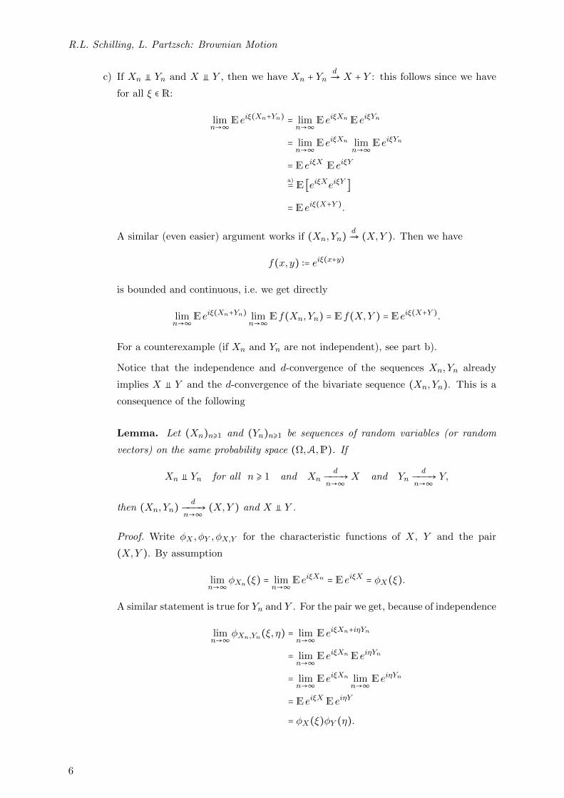
Problem 2.6 (Solution) We use formula (2.10b).

a) fB(s),B(t)(x, y) =1

2π√s(t − s)

exp [−1

2(x

2

s+ (y − x)2

t − s )] .

b) Denote by fB(1) the density of B(1). Then we have

fB(s),B(t) ∣B(1)(x, y∣B(1) = z)

=fB(s),B(t),B(1)(x, y, z)

fB(1)(z)

= 1

(2π)3/2√s(t − s)(1 − t)

exp [−1

2(x

2

s+ (y − x)2

t − s + (z − y)2

1 − t )] (2π)1/2 exp [z2

2] .

Thus,

fB(s),B(t)∣B(1)(x, y ∣B(1) = 0) = 1

2π√s(t − s)(1 − t)

exp [−1

2(x

2

s+ (y − x)2

t − s + y2

1 − t)] .

Note that

x2

s+ (y − x)2

t − s + y2

1 − t =t

s(t − s) (x − sty)

2

+ y2

t+ y2

1 − t =t

s(t − s) (x − sty)

2

+ y2

t(1 − t) .

Therefore,

E(B(s)B(t) ∣B(1) = 0)

=∬ xyfB(s),B(t)∣B(1)(x, y ∣B(1) = 0)dxdy

= 1

2π√s(t − s)(1 − t) ∫

∞

y=−∞y exp [−1

2

y2

t(1 − t)]×

× ∫∞

x=−∞x exp [−1

2

t

s(t − s) (x − sty)

2

] dx´¹¹¹¹¹¹¹¹¹¹¹¹¹¹¹¹¹¹¹¹¹¹¹¹¹¹¹¹¹¹¹¹¹¹¹¹¹¹¹¹¹¹¹¹¹¹¹¹¹¹¹¹¹¹¹¹¹¹¹¹¹¹¹¹¹¹¹¹¹¹¹¹¹¹¹¹¹¹¹¹¹¹¹¹¹¹¹¹¹¹¹¹¹¹¹¹¹¹¹¹¹¹¹¹¹¹¹¹¹¹¹¹¹¹¹¹¹¹¹¹¹¹¹¹¹¹¹¹¹¹¹¹¹¹¹¹¸¹¹¹¹¹¹¹¹¹¹¹¹¹¹¹¹¹¹¹¹¹¹¹¹¹¹¹¹¹¹¹¹¹¹¹¹¹¹¹¹¹¹¹¹¹¹¹¹¹¹¹¹¹¹¹¹¹¹¹¹¹¹¹¹¹¹¹¹¹¹¹¹¹¹¹¹¹¹¹¹¹¹¹¹¹¹¹¹¹¹¹¹¹¹¹¹¹¹¹¹¹¹¹¹¹¹¹¹¹¹¹¹¹¹¹¹¹¹¹¹¹¹¹¹¹¹¹¹¹¹¹¹¹¹¹¹¶

=√s(t−s)√t

√2π s

ty

dy

= 1√2π

√t(1 − t) ∫

∞

y=−∞y2 s

texp [−1

2

y2

t(1 − t)] dy

= stt(1 − t) = s(1 − t).

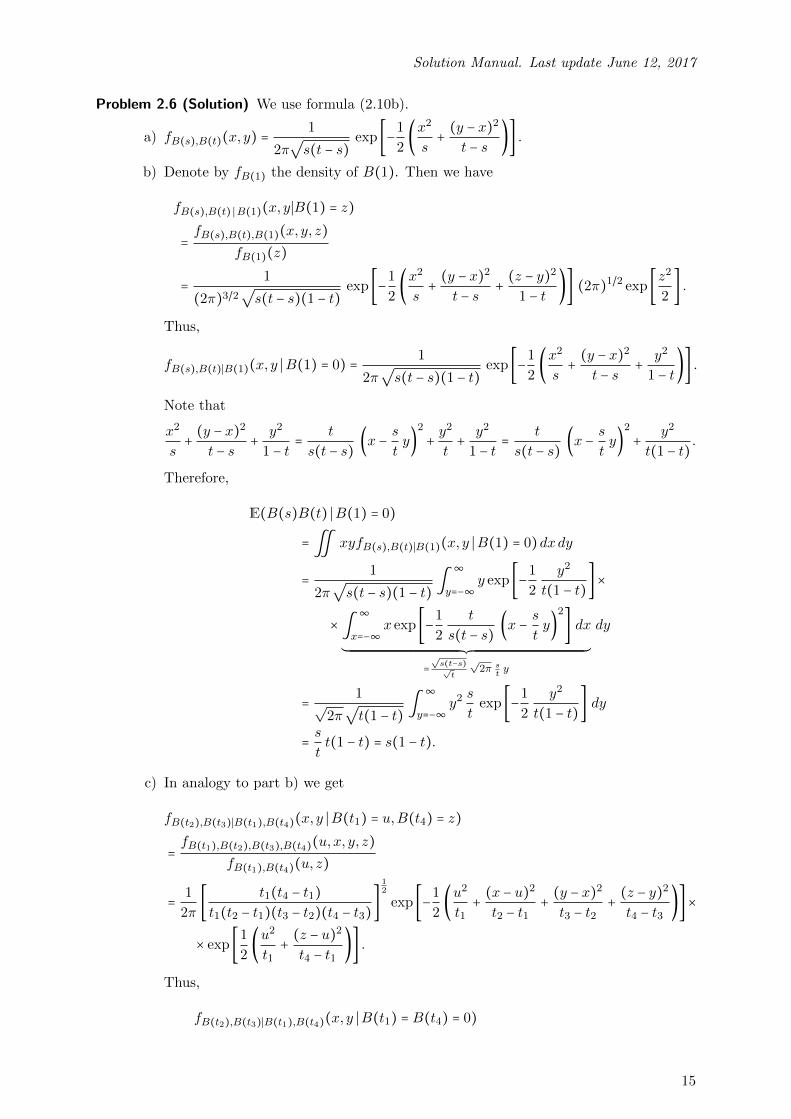
c) In analogy to part b) we get

fB(t2),B(t3)∣B(t1),B(t4)(x, y ∣B(t1) = u,B(t4) = z)

=fB(t1),B(t2),B(t3),B(t4)(u,x, y, z)

fB(t1),B(t4)(u, z)

= 1

2π[ t1(t4 − t1)t1(t2 − t1)(t3 − t2)(t4 − t3)

]12

exp [−1

2(u

2

t1+ (x − u)2

t2 − t1+ (y − x)2

t3 − t2+ (z − y)2

t4 − t3)]×

× exp [1

2(u

2

t1+ (z − u)2

t4 − t1)] .

Thus,

fB(t2),B(t3)∣B(t1),B(t4)(x, y ∣B(t1) = B(t4) = 0)

15


= 1

2π[ t1(t4 − t1)t1(t2 − t1)(t3 − t2)(t4 − t3)

]12

exp [−1

2( x2

t2 − t1+ (y − x)2

t3 − t2+ y2

t4 − t3)] .

Observe that

x2

t2 − t1+ (y − x)2

t3 − t2+ y2

t4 − t3= t3 − t1

(t2 − t1)(t3 − t2)(x − t2 − t1

t3 − t1y)

2

+ t4 − t1(t3 − t1)(t4 − t3)

y2.

Therefore, we get (using physicists’ notation: ∫ dy h(y) ∶= ∫ h(y)dy for easier read-

ability)

∬ xy fB(t2),B(t3)∣B(t1),B(t4)(x, y ∣B(t1) = B(t4) = 0)dxdy

= 1

2π(t4 − t3) ∫∞

y=−∞dy exp [−1

2

t4 − t1(t3 − t1)(t4 − t3)

y2]×

× y√2π(t2 − t1)(t3 − t2)

∫∞

x=−∞x exp [−1

2(x − t2 − t1

t3 − t1y)

2 t3 − t1(t2 − t1)(t3 − t2)

] dx

´¹¹¹¹¹¹¹¹¹¹¹¹¹¹¹¹¹¹¹¹¹¹¹¹¹¹¹¹¹¹¹¹¹¹¹¹¹¹¹¹¹¹¹¹¹¹¹¹¹¹¹¹¹¹¹¹¹¹¹¹¹¹¹¹¹¹¹¹¹¹¹¹¹¹¹¹¹¹¹¹¹¹¹¹¹¹¹¹¹¹¹¹¹¹¹¹¹¹¹¹¹¹¹¹¹¹¹¹¹¹¹¹¹¹¹¹¹¹¹¹¹¹¹¹¹¹¹¹¹¹¹¹¹¹¹¹¹¹¹¹¹¹¹¹¹¹¹¹¹¹¹¹¹¹¹¹¹¹¹¹¹¹¹¹¹¹¹¹¹¹¹¹¹¹¹¹¹¹¹¹¹¹¹¹¹¹¹¹¹¹¹¹¹¹¹¹¹¹¹¹¹¹¹¹¹¹¹¹¹¹¹¹¹¹¹¹¹¹¹¹¹¹¹¹¹¹¹¹¹¹¹¹¹¹¹¹¹¹¹¹¹¹¹¹¹¹¹¹¹¹¹¹¹¹¹¹¹¹¹¹¹¹¹¹¹¹¹¹¹¹¹¹¹¸¹¹¹¹¹¹¹¹¹¹¹¹¹¹¹¹¹¹¹¹¹¹¹¹¹¹¹¹¹¹¹¹¹¹¹¹¹¹¹¹¹¹¹¹¹¹¹¹¹¹¹¹¹¹¹¹¹¹¹¹¹¹¹¹¹¹¹¹¹¹¹¹¹¹¹¹¹¹¹¹¹¹¹¹¹¹¹¹¹¹¹¹¹¹¹¹¹¹¹¹¹¹¹¹¹¹¹¹¹¹¹¹¹¹¹¹¹¹¹¹¹¹¹¹¹¹¹¹¹¹¹¹¹¹¹¹¹¹¹¹¹¹¹¹¹¹¹¹¹¹¹¹¹¹¹¹¹¹¹¹¹¹¹¹¹¹¹¹¹¹¹¹¹¹¹¹¹¹¹¹¹¹¹¹¹¹¹¹¹¹¹¹¹¹¹¹¹¹¹¹¹¹¹¹¹¹¹¹¹¹¹¹¹¹¹¹¹¹¹¹¹¹¹¹¹¹¹¹¹¹¹¹¹¹¹¹¹¹¹¹¹¹¹¹¹¹¹¹¹¹¹¹¹¹¹¹¹¹¹¹¹¹¹¹¹¹¹¹¹¹¹¹¹¶= y2√

t3−t1t2−t1t3−t1

= t2 − t1t3 − t1

(t4 − t3)(t3 − t1)t4 − t1

= (t2 − t1)(t4 − t3)t4 − t1

.

Problem 2.7 (Solution) Let s ⩽ t. Then

C(s, t) = E(XsXt)

= E(B2s − s)(B2

t − t)

= E(B2s − s)([Bt −Bs +Bs]2 − t)

= E(B2s − s)(Bt −Bs)2 + 2E(B2

s − s)Bs(Bt −Bs) +E(B2s − s)B2

s −E(B2s − s)t

(B1)= E(B2s − s)E(Bt −Bs)2 + 2E(B2

s − s)BsE(Bt −Bs) +E(B2s − s)B2

s −E(B2s − s)t

= 0 ⋅ (t − s) + 2E(B2s − s)Bs ⋅ 0 +EB4

s − sEB2s − 0

= 2s2 = 2(s2 ∧ t2) = 2(s ∧ t)2.

Problem 2.8 (Solution) a) We have for s, t ⩾ 0

m(t) = EXt = e−αt/2EBeαt = 0.

C(s, t) = E(XsXt) = e−α2(s+t)EBeαsBeαt = e−

α2(s+t)(eαs ∧ eαt) = e−

α2∣t−s∣.

b) We have

P(X(t1) ⩽ x1, . . . ,X(tn) ⩽ xn) = P (B(eαt1) ⩽ eαt1/2x1, . . . ,B(eαtn) ⩽ eαtn/2xn)

Thus, the density is

fX(t1),...,X(tn)(x1, . . . , xn)

=n

∏k=1

eαtk/2fB(eαt1),...,B(eαtn)(eαt1/2x1, . . . , eαtn/2xn)

16


=n

∏k=1

eαtk/2(2π)−n/2 (n

∏k=1

(eαtk − eαtk−1))−1/2

e−12 ∑

nk=1(eαtk/2xk−eαtk−1/2xk−1)2/(eαtk−eαtk−1)

= (2π)−n/2 (n

∏k=1

(1 − e−α(tk−tk−1)))−1/2

e−12 ∑

nk=1(xk−e−α(tk−tk−1)/2xk−1)2/(1−eα(tk−tk−1))

(we use the convention t0 = −∞ and x0 = 0).

Remark: the form of the density shows that the Ornstein–Uhlenbeck is strictly stationary,

i.e.

(X(t1 + h), . . . ,X(tn + h) ∼ (X(t1), . . . ,X(tn)) ∀h > 0.

Problem 2.9 (Solution) “⇒” Assume that we have (B1). Observe that the family of sets

⋃0⩽u1⩽⋯⩽un⩽s, n⩾1

σ(Bu1 , . . . ,Bun)

is a ∩-stable family. This means that it is enough to show that

Bt −Bs á (Bu1 , . . . ,Bun) for all t ⩾ s ⩾ 0.

By (B1) we know that

Bt −Bs á (Bu1 ,Bu2 −Bu1 , . . . ,Bun −Bun−1)

and so

Bt −Bs á

⎛⎜⎜⎜⎜⎜⎜⎜⎜⎜⎝

1 0 0 . . . 0

1 1 0 . . . 0

1 1 1 . . . 0

⋮ ⋮ ⋮ ⋱ 0

1 1 1 . . . 1

⎞⎟⎟⎟⎟⎟⎟⎟⎟⎟⎠

⎛⎜⎜⎜⎜⎜⎜⎜⎜⎜⎝

Bu1

Bu2 −Bu1Bu3 −Bu2

⋮Bun −Bun−1

⎞⎟⎟⎟⎟⎟⎟⎟⎟⎟⎠

=

⎛⎜⎜⎜⎜⎜⎜⎜⎜⎜⎝

Bu1

Bu2

Bu3

⋮Bun

⎞⎟⎟⎟⎟⎟⎟⎟⎟⎟⎠

“⇐” Let 0 = t0 ⩽ t1 < t2 < . . . < tn <∞, n ⩾ 1. Then we find for all ξ1, . . . , ξn ∈ Rd

E (ei∑nk=1⟨ξk, B(tk)−B(tk−1)⟩) = E (ei⟨ξn, B(tn)−B(tn−1)⟩ ⋅ ei∑n−1k=1 ⟨ξk, B(tk)−B(tk−1)⟩´¹¹¹¹¹¹¹¹¹¹¹¹¹¹¹¹¹¹¹¹¹¹¹¹¹¹¹¹¹¹¹¹¹¹¹¹¹¹¹¹¹¹¹¹¹¹¹¹¹¹¹¹¹¹¹¹¹¹¹¹¹¹¹¹¹¹¹¸¹¹¹¹¹¹¹¹¹¹¹¹¹¹¹¹¹¹¹¹¹¹¹¹¹¹¹¹¹¹¹¹¹¹¹¹¹¹¹¹¹¹¹¹¹¹¹¹¹¹¹¹¹¹¹¹¹¹¹¹¹¹¹¹¹¹¹¹¶

Ftn−1 mble., hence áB(tn)−B(tn−1))

= E (ei⟨ξn, B(tn)−B(tn−1)⟩) ⋅E (ei∑n−1k=1 ⟨ξk, B(tk)−B(tk−1)⟩)

⋮

=n

∏k=1

E (ei⟨ξk, B(tk)−B(tk−1)⟩).

This shows (B1).

Problem 2.10 (Solution) Reflection invariance of BM, cf. 2.8, shows

τa = infs ⩾ 0 ∶ Bs = a ∼ infs ⩾ 0 ∶ −Bs = a = infs ⩾ 0 ∶ Bs = −a = τ−a.

The scaling property 2.12 of BM shows for c = 1/a2

τa = infs ⩾ 0 ∶ Bs = a ∼ infs ⩾ 0 ∶ aBs/a2 = a

= infa2r ⩾ 0 ∶ aBr = a

= a2 infr ⩾ 0 ∶ Br = 1 = a2τ1.

17


Problem 2.11 (Solution) a) Not stationary:

EW 2t = C(t, t) = E(B2

t − t)2 = E(B4t − 2tB2

t + t2) = 3t2 − 2t2 + t2 = 2t2 ≠ const.

b) Stationary. We have EXt = 0 and

EXsXt = e−α(t+s)/2EBeαsBeαt = e−α(t+s)/2(eαs ∧ eαt) = e−α∣t−s∣/2,

i.e. it is stationary with g(r) = e−α∣r∣/2.

c) Stationary. We have EYt = 0. Let s ⩽ t. Then we use EBsBt = s ∧ t to get

EYsYt = E(Bs+h −Bs)(Bt+h −Bt)

= EBs+hBt+h −EBs+hBt −EBsBt+h +EBsBt= (s + h) ∧ (t + h) − (s + h) ∧ t − s ∧ (t + h) + s ∧ t

= (s + h) − (s + h) ∧ t =⎧⎪⎪⎪⎨⎪⎪⎪⎩

0, if t > s + h ⇐⇒ h < t − s

h − (t − s), if t ⩽ s + h ⇐⇒ h ⩾ t − s.

Swapping the roles of s and t finally gives: the process is stationary with g(t) =(h − ∣t∣)+ = (h − ∣t∣) ∨ 0.

d) Not stationary. Note that

EZ2t = EB2

et = et ≠ const.

Problem 2.12 (Solution) Clearly, t↦Wt is continuous for t ≠ 1. If t = 1 we get

limt↑1

Wt(ω) =W1(ω) = B1(ω)

and

limt↓1

Wt(ω) = B1(ω) − limt↓1

tβ1/t(ω) − β1(ω) = B1(ω);

this proves continuity for t = 1.

Let us check that W is a Gaussian process with EWt = 0 and EWsWt = s ∧ t. By

Corollary 2.7, W is a BM1.

Pick n ⩾ 1 and t0 = 0 < t1 < . . . < tn.

Case 1: If tn ⩽ 1, there is nothing to show since (Bt)t∈[0,1] is a BM1.

Case 2: Assume that tn > 1. Then we have

⎛⎜⎜⎜⎜⎜⎜⎝

Wt1

Wt2

⋮Wtn

⎞⎟⎟⎟⎟⎟⎟⎠

=

⎛⎜⎜⎜⎜⎜⎜⎝

1 t1 0 0 ⋯ 0 −1

1 0 t2 0 ⋯ 0 −1

⋮ ⋮ 0 t3 ⋯ ⋮ ⋮1 0 0 0 ⋯ tn −1

⎞⎟⎟⎟⎟⎟⎟⎠

⎛⎜⎜⎜⎜⎜⎜⎜⎜⎜⎝

B1

β1/t1⋮

β1/tnβ1

⎞⎟⎟⎟⎟⎟⎟⎟⎟⎟⎠

18


and since

B1 á (β1/t1 , . . . , β1/tn , β1)⊺

are both Gaussian, we see that (Wt1 , . . . ,Wtn) is Gaussian.

Further, let t ⩾ 1 and 1 ⩽ ti < tj :

EWt = EB1 + tEβ1/t −Eβ1 = 0

EWtiWtj = E(B1 + tiβ1/ti − β1)(B1 + tjβ1/tj − β1)

= 1 + titjt−1j − tit−1

i − tjt−1j + 1 = ti = ti ∧ tj .

Case 3: Assume that 0 < t1 < . . . < tk ⩽ 1 < tk+1 < . . . < tn. Then we have

⎛⎜⎜⎜⎜⎜⎜⎜⎜⎜⎜⎜⎜⎝

Wt1

Wt2

⋮Wtk

⋮Wtn

⎞⎟⎟⎟⎟⎟⎟⎟⎟⎟⎟⎟⎟⎠

=

⎛⎜⎜⎜⎜⎜⎜⎜⎜⎜⎜⎜⎜⎜⎜⎜⎜⎜⎜⎜⎝

1 0 ⋯ 0

0 ⋱ 0

⋮ ⋱ ⋮0 0 ⋯ 1

1 tk+1 0 ⋯ 0 −1

1 0 tk+2 0 −1

⋮ ⋮ ⋱ ⋮1 0 ⋯ tn −1

⎞⎟⎟⎟⎟⎟⎟⎟⎟⎟⎟⎟⎟⎟⎟⎟⎟⎟⎟⎟⎠

⎛⎜⎜⎜⎜⎜⎜⎜⎜⎜⎜⎜⎜⎜⎜⎜⎜⎜⎜⎜⎜⎜⎜⎝

Bt1

⋮⋮Btk

B1

β1/tk+1⋮

β1/tnβ1

⎞⎟⎟⎟⎟⎟⎟⎟⎟⎟⎟⎟⎟⎟⎟⎟⎟⎟⎟⎟⎟⎟⎟⎠

.

Since

(Bt1 , . . . ,Btk ,B1) á (β1/tk+1 , . . . , β1/tn , β1)

are Gaussian vectors, (Wt1 , . . . ,Wtn) is also Gaussian and we find

EWt = 0

EWtiWtj = EBti(B1 + tjβ1/tj − β1) = ti = ti ∧ tj

for i ⩽ k < j.

Problem 2.13 (Solution) The process X(t) = B(et) has no memory since (cf. Problem 2.9)

σ(B(s) ∶ s ⩽ ea) á σ(B(s) −B(ea) ∶ s ⩾ ea)

and, therefore,

σ(X(t) ∶ t ⩽ a) = σ(B(s) ∶ 1 ⩽ s ⩽ ea) á σ(B(ea+s) −B(ea) ∶ s ⩾ 0)

= σ(X(t + a) −X(a) ∶ t ⩾ 0).

The process X(t) ∶= e−t/2B(et) is not memoryless. For example, X(a + a) −X(a) is not

independent of X(a):

E(X(2a) −X(a))X(a) = E (e−aB(e2a) − e−a/2B(ea))e−a/2B(ea) = e−3a/2ea − e−aea ≠ 0.

19


Problem 2.14 (Solution) The process Wt = Ba−t −Ba,0 ⩽ t ⩽ a clearly satisfies (B0) and (B4).

For 0 ⩽ s ⩽ t ⩽ a we find

Wt −Ws = Ba−t −Ba−s ∼ Ba−s −Ba−t ∼ Bt−s ∼ N(0, (t − s) id)

and this shows (B2) and (B3).

For 0 = t0 < t1 < . . . < tn ⩽ a we have

Wtj −Wtj−1 = Ba−tj −Ba−tj−1 ∼ Ba−tj−1 −Ba−tj ∀j

and this proves that W inherits (B1) from B.

Problem 2.15 (Solution) We know from Paragraph 2.13 that

limt↓0

tB(1/t) = 0 Ô⇒ lims↑∞

B(s)s

= 0 a.s.

Moreover,

E(B(s)s

)2

= s

s2= 1

s

s→∞ÐÐÐ→ 0

i.e. we get also convergence in mean square.

Remark: a direct proof of the SLLN is a bit more tricky. Of course we have by the classical

SLLN thatBnn

=∑nj=1(Bj −Bj−1)

n

SLLNÐÐÐ→n→∞

0 a.s.

But then we have to make sure that Bs/s converges. This can be done in the following

way: fix s > 0. Then there is a unique interval (n,n + 1] such that s ∈ (n,n + 1]. Thus,

∣Bss

∣ ⩽ ∣Bs −Bn+1

s∣ + ∣Bn+1

n + 1∣ ⋅ n + 1

s⩽ supn⩽s⩽n+1 ∣Bs −Bn+1∣

n+ n + 1

n∣Bnn

∣

and we have to show that the expression with the sup tends to zero. This can be done

by showing, e.g., that the L2-limit of this expression goes to zero (using the reflection

principle) and with a subsequence argument.

Problem 2.16 (Solution) Set

Σ ∶= ⋃J⊂[0,∞), J countable

σ(B(t) ∶ t ∈ J)

Clearly,

⋃t⩾0

σ(Bt) ⊂ Σ ⊂ σ(Bt ∶ t ⩾ 0) def= FB∞ (*)

The first inclusion follows from the fact that each Bt is measurable with respect to Σ.

Let us show that Σ is a σ-algebra. Obviously,

∅ ∈ Σ and F ∈ Σ Ô⇒ F c ∈ Σ.

20


Let (An)n ⊂ Σ. Then, for every n there is a countable set Jn such that An ∈ σ(B(t) ∶ t ∈Jn). Since J = ⋃n Jn is still countable we see that An ∈ σ(B(t) ∶ t ∈ J) for all n. Since

the latter family is a σ-algebra, we find

⋃nAn ∈ σ(B(t) ∶ t ∈ J) ⊂ Σ.

Since ⋃t σ(Bt) ⊂ Σ, we get—note: FB∞ is, by definition, the smallest σ-algebra for which

all Bt are measurable—that

FB∞ ⊂ Σ.

This shows that Σ = FB∞.

Problem 2.17 (Solution) Assume that the indices t1, . . . , tm and s1, . . . , sn are given. Let

u1, . . . , up ∶= s1, . . . , sn ∪ t1, . . . , tm. By assumption,

(X(u1), . . . ,X(up)) á (Y (u1), . . . , Y (up)).

Thus, we may thin out the indices on each side without endangering independence:

s1, . . . , sn ⊂ u1, . . . , up and t1, . . . , tm ⊂ u1, . . . , up, and so

(X(s1), . . . ,X(sn)) á (Y (t1), . . . , Y (tm)).

Problem 2.18 (Solution) Since Ft ⊂ F∞ and Gt ⊂ G∞ it is clear that

F∞ á G∞ Ô⇒ Ft á Gt.

Conversely, since (Ft)t⩾0 and (Gt)t⩾0 are filtrations we find

∀F ∈ ⋃t⩾0

Ft, ∀G ∈ ⋃t⩾0

Gt, ∃t0 ∶ F ∈ Ft0 , G ∈ Gt0 .

By assumption: P(F ∩G) = P(F )P(G). Thus,

⋃t⩾0

Ft á ⋃t⩾0

Gt.

Since the families ⋃t⩾0 Ft and ⋃t⩾0 Gt are ∩-stable (use again the argument that we have

filtrations to find for F,F ′ ∈ ⋃t⩾0 Ft some t0 with F,F ′ ∈ Ft0 etc.), the σ-algebras generated

by these families are independent:

F∞ = σ (⋃t⩾0

Ft) á σ (⋃t⩾0

Gt) = G∞.

Problem 2.19 (Solution) Let U ∈ Rd×d be an orthogonal matrix: UU⊺ = id and set Xt ∶= UBtfor a BMd (Bt)t⩾0. Then

E⎛⎝

exp

⎡⎢⎢⎢⎢⎣in

∑j=1

⟨ξj , X(tj) −X(tj−1)⟩⎤⎥⎥⎥⎥⎦

⎞⎠= E

⎛⎝

exp

⎡⎢⎢⎢⎢⎣in

∑j=1

⟨ξj , UB(tj) −UB(tj−1)⟩⎤⎥⎥⎥⎥⎦

⎞⎠

21


= E⎛⎝

exp

⎡⎢⎢⎢⎢⎣in

∑j=1

⟨U⊺ξj , B(tj) −B(tj−1)⟩⎤⎥⎥⎥⎥⎦

⎞⎠

= exp

⎡⎢⎢⎢⎢⎣−1

2

n

∑j=1

(tj − tj−1)⟨U⊺ξj , U⊺ξj⟩

⎤⎥⎥⎥⎥⎦

= exp

⎡⎢⎢⎢⎢⎣−1

2

n

∑j=1

(tj − tj−1)∣ξj ∣2⎤⎥⎥⎥⎥⎦.

(Observe ⟨U⊺ξj , U⊺ξj⟩ = ⟨UU⊺ξj , ξj⟩ = ⟨ξj , ξj⟩ = ∣ξj ∣2). The claim follows.

Problem 2.20 (Solution) Note that the coordinate processes b and β are independent BM1.

a) Since b á β, the process Wt = (bt + βt)/√

2 is a Gaussian process with continuous

sample paths. We determine its mean and covariance functions:

EWt =1√2(E bt +Eβt) = 0;

Cov(Ws,Wt) = E(WsWt)

= 1

2E(bs + βs)(bt + βt)

= 1

2(E bsbt +Eβsbt +E bsβt +Eβsβt)

= 1

2(s ∧ t + 0 + 0 + s ∧ t) = s ∧ t

where we used that, by independence, E buβv = E buEβv = 0. Now the claim follows

from Corollary 2.7.

b) The process Xt = (Wt, βt) has the following properties

• W and β are BM1

• E(Wtbt) = 2−1/2E(bt+βt)βt = 2−1/2(E btEβt+Eβ2t ) = t/

√2 ≠ 0, i.e. W and β are

NOT independent.

This means that X is not a BM2, as its coordinates are not independent.

The process Yt can be written as

1√2

⎛⎝bt + βtbt − βt

⎞⎠= U

⎛⎝bt

βt

⎞⎠= 1√

2

⎛⎝

1 1

1 −1

⎞⎠⎛⎝bt

βt

⎞⎠.

Clearly, UU⊺ = id, i.e. Problem 2.19 shows that (Yt)t⩾0 is a BM2.

Problem 2.21 (Solution) Observe that b á β since B is a BM2. Since

EXt = 0

Cov(Xt,Xs) = EXtXs

= E(λbs + µβs)(λbt + µβt)

= λ2E bsbt + λµE bsβt + λµE btβs + µ2βsβt

22


= λ2E bsbt + λµE bsEβt + λµE btEβs + µ2Eβsβt

= λ2(s ∧ t) + 0 + 0 + µ2s ∧ t = (λ2 + µ2)(s ∧ t).

Thus, by Corollary 2.7, X is a BM1 if, and only if, λ2 + µ2 = 1.

Problem 2.22 (Solution) Xt = (bt, βs−t − βt), 0 ⩽ t ⩽ s, is NOT a Brownian motion: X0 =(0, βs) ≠ (0,0).

On the other hand, Yt = (bt, βs−t − βs), 0 ⩽ t ⩽ s, IS a Brownian motion, since bt and

βs−t − βs are independent BM1, cf. Time inversion 2.11 and Theorem 2.16.

Problem 2.23 (Solution) We have

Wt = UB⊺t =

⎛⎝

cosα sinα

− sinα cosα

⎞⎠⎛⎝bt

βt

⎞⎠.

The matrix U is a rotation, hence orthogonal and we see from Problem 2.19 that W is a

Brownian motion.

Generalization: take U orthogonal.

Problem 2.24 (Solution) IfG ∼ N(0,Q) thenQ is the covariance matrix, i.e. Cov(Gj ,Gk) = qjk.Thus, we get for s < t

Cov(Xjs ,X

kt ) = E(Xj

sXkt )

= EXjs(Xk

t −Xks ) +E(Xj

sXks )

= EXjs E(Xk

t −Xks ) + sqjk

= (s ∧ t)qjk.

The characteristic function is

E ei⟨ξ,Xt⟩ = E ei⟨Σ⊺ξ,Bt⟩ = e− t2 ∣Σ⊺ξ∣2 = e− t2 ⟨ξ,ΣΣ⊺ξ⟩,

and the transition probability is, if Q is non-degenerate,

fQ(x) =1√

(2πt)ndetQexp(− 1

2t⟨x,Qx⟩) .

If Q is degenerate, there is an orthogonal matrix U ∈ Rn×n such that

UXt = (Y 1t , . . . , Y

kt ,0, . . . ,0´¹¹¹¹¹¹¹¹¹¸¹¹¹¹¹¹¹¹¹¶

n−k

)⊺

where k < n is the rank of Q. The k-dimensional vector has a nondegenerate normal

distribution in Rk.

23

3 Constructions of Brownian Motion

Problem 3.1 (Solution) The partial sums

WN(t, ω) =N−1

∑n=0

Gn(ω)Sn(t), t ∈ [0,1],

converge as N → ∞ P-a.s. uniformly for t towards B(t, ω), t ∈ [0,1]—cf. Problem 3.2.

Therefore, the random variables

∫1

0WN(t)dt =

N−1

∑n=0

Gn∫1

0Sn(t)dt

P -a.s.ÐÐÐ→N→∞

X = ∫1

0B(t)dt.

This shows that ∫ 10 WN(t)dt is the sum of independent N(0,1)-random variables, hence

itself normal and so is its limit X.

From the definition of the Schauder functions (cf. Figure 3.2) we find

∫1

0S0(t)dt =

1

2

∫1

0S2j+k(t)dt =

1

42−

32j , k = 0,1, . . . ,2j − 1, j ⩾ 0.

and this shows

∫1

0W2n+1(t)dt =

1

2G0 +

1

4

n

∑j=0

2j−1

∑l=0

2−32jG2j+l.

Consequently, since the Gj are iid N(0,1) random variables,

E∫1

0W2n+1(t)dt = 0,

V∫1

0W2n+1(t)dt =

1

4+ 1

16

n

∑j=0

2j−1

∑l=0

2−3j

= 1

4+ 1

16

n

∑j=0

2−2j

= 1

4+ 1

16

1 − 2−2(n+1)

1 − 14

ÐÐÐ→n→∞

1

4+ 1

16

4

3= 1

3.

This means that

X = 1

2G0 +

∞∑j=0

1

42−

32j

2j−1

∑l=0

G2j+l

´¹¹¹¹¹¹¹¹¹¹¹¹¹¹¹¹¹¸¹¹¹¹¹¹¹¹¹¹¹¹¹¹¹¹¹¶∼N(0,2j)

where the series converges P-a.s. and in mean square, and X ∼ N(0, 13).

25


Problem 3.2 (Solution) a) From the definition of the Schauder functions Sn(t), n ⩾ 0, t ∈[0,1], we find

0 ⩽ Sn(t) ∀n, t

S2j+k(t) ⩽ S2j+k((2k + 1)/2j+1) = 2−j/2/2j+1 = 1

22−j/2 ∀j, k, t

2j−1

∑k=0

S2j+k(t) ⩽1

22−j/2 (disjoint supports!)

By assumption,

∃C > 0, ∃ε ∈ (0, 12), ∀n ∶ ∣an∣ ⩽ C ⋅ nε.

Thus, we find

∞∑n=0

∣an∣Sn(t) ⩽ ∣a0∣ +∞∑j=0

2j−1

∑k=0

∣a2j+k∣S2j+k(t)

⩽ ∣a0∣ +∞∑j=0

2j−1

∑k=0

C ⋅ (2j+1)ε S2j+k(t)

⩽ ∣a0∣ +∞∑j=0

C ⋅ 2(j+1)ε 1

22−j <∞.

(The series is convergent since ε < 1/2).

This shows that ∑∞n=0 anSn(t) converges absolutely and uniformly for t ∈ [0,1].

b) For C >√

2 we find from

P (∣Gn∣ >√

logn) ⩽√

2

π

1

C√

logne−

12C2 logn ⩽

√2

π

1

Cn−C

2/2 ∀n ⩾ 3

that the following series converges:

∞∑n=1

P (∣Gn∣ >√

logn) <∞.

By the Borel–Cantelli Lemma we find that Gn(ω) = O(√

logn) for almost all ω, thus

Gn(ω) = O(nε) for any ε ∈ (0,1/2).

From part a) we know that the series ∑∞n=0Gn(ω)Sn(t) converges a.s. uniformly for

t ∈ [0,1].

Problem 3.3 (Solution) Set ∥f∥p ∶= (E ∣f ∣p)1/p

Solution 1: We observe that the space Lp(Ω,A,P;S) = X ∶ X ∈ S, ∥d(X,0)∥p < ∞ is

complete and that the condition stated in the problem just says that (Xn)n is a Cauchy

sequence in the space Lp(Ω,A,P;S). A good reference for this is, for example, the mono-

graph by F. Treves [13, Chapter 46]. You will find the ‘pedestrian’ approach as Solution

2 below.

26


Solution 2: By assumption

∀k ⩾ 0 ∃Nk ⩾ 1 ∶ supm⩾Nk

∥d(XNk ,Xm)∥p ⩽ 2−k.

Without loss of generality we can assume that Nk ⩽ Nk+1. In particular

∥d(XNk ,XNk+1)∥p ⩽ 2−k∀l>kÔ⇒ ∥d(XNk ,XNl)∥p ⩽

l−1

∑j=k

2−j ⩽ 2

2k.

Fix m ⩾ 1. Then we see that

∥d(XNk ,Xm) − d(XNl ,Xm)∥p ⩽ ∥d(XNk ,XNl)∥p ÐÐÐ→k,l→∞

0.

This means that that (d(XNk ,Xm))k⩾0 is a Cauchy sequence in Lp(P;R). By the com-

pleteness of the space Lp(P;R) there is some fm ∈ Lp(P;R) such that

d(XNk ,Xm) in LpÐÐÐ→k→∞

fm

and, for a subsequence (nk) ⊂ (Nk)k we find

d(Xnk ,Xm) almost surelyÐÐÐÐÐÐÐ→k→∞

fm.

The subsequence nk may also depend on m. Since (nk(m))k is still a subsequence of

(Nk), we still have d(Xnk(m),Xm+1) → fm+1 in Lp, hence we can find a subsequence

(nk(m + 1))k ⊂ (nk(m))k such that d(Xnk(m+1),Xm+1) → fm+1 a.s. Iterating this we see

that we can assume that (nk)k does not depend on m.

In particular, we have almost surely

∀ε > 0 ∃L = L(ε) ⩾ 1 ∀k ⩾ L ∶ ∣d(Xnk ,Xm) − fm∣ ⩽ ε.

Moreover,

limm→∞

∥fm∥p = limm→∞

∥ limk→∞

d(Xnk ,Xm)∥p ⩽ limm→∞

limk→∞

∥d(Xnk ,Xm)∥p

⩽ limk→∞

supm⩾nk

∥d(Xnk ,Xm)∥p = 0.

Thus, fm → 0 in Lp and, for a subsequence mk we get

∀ε > 0 ∃K =K(ε) ⩾ 1 ∀r ⩾K ∶ ∣fmr ∣ ⩽ ε.

Therefore,

d(Xnk ,Xnl) ⩽ d(Xnk ,Xmr) + d(Xnk ,Xmr)

⩽ ∣d(Xnk ,Xmr) − fmr ∣ + ∣d(Xnk ,Xmr) − fmr ∣ + 2∣fmr ∣.

Fix ε > 0 and pick r >K. Then let k, l →∞. This gives

d(Xnk ,Xnl) ⩽ ∣d(Xnk ,Xmr) − fmr ∣ + ∣d(Xnk ,Xmr) − fmr ∣ + 2ε ⩽ 4ε ∀k, l ⩾ L(ε).

27


Since S is complete, this proves that (Xnk)k⩾0 converges to some X ∈ S almost surely.

Remark: If we replace the condition of the Problem by

limn→∞

E(supm⩾n

dp(Xn,Xm)) = 0

things become MUCH simpler:

This condition says that the sequence dn ∶= supm⩾n dp(Xn,Xm) converges in Lp(P;R) to

zero. Hence there is a subsequence (nk)k such that

limk→∞

supm⩾nk

d(Xnk ,Xm) = 0

almost surely. This shows that d(Xnk ,Xnl)→ 0 as k, l →∞, i.e. we find by the complete-

ness of the space S that Xnk →X.

Problem 3.4 (Solution) Fix n ⩾ 1, 0 ⩽ t1 ⩽ . . . ⩽ tn and Borel sets A1, . . . ,An. By assumption,

we know that

P(Xt = Yt) = 1 ∀t ⩾ 0 Ô⇒ P(Xtj = Ytj j = 1, . . . , n) = P⎛⎝n

⋂j=1

Xtj = Ytj⎞⎠= 1.

Thus,

P⎛⎝n

⋂j=1

Xtj ∈ Aj⎞⎠= P

⎛⎝n

⋂j=1

Xtj ∈ Aj ∩n

⋂j=1

Xtj = Ytj⎞⎠

= P⎛⎝n

⋂j=1

Xtj ∈ Aj ∩ Xtj = Ytj⎞⎠

= P⎛⎝n

⋂j=1

Ytj ∈ Aj ∩ Xtj = Ytj⎞⎠

= P⎛⎝n

⋂j=1

Ytj ∈ Aj⎞⎠.

Problem 3.5 (Solution) indistinguishable Ô⇒ modification:

P(Xt = Yt ∀t ⩾ 0) = 1 Ô⇒ ∀t ⩾ 0 ∶ P(Xt = Yt) = 1.

modification Ô⇒ equivalent: see the previous Problem 3.4

Now assume that I is countable or t↦Xt, t↦ Yt are (left- or right-)continuous.

modification Ô⇒ indistinquishable: By assumption, P(Xt ≠ Yt) = 0 for any t ∈ I. Let

D ⊂ I be any countable dense subset. Then

P⎛⎝⋃q∈D

Xq ≠ Yq⎞⎠⩽ ∑q∈D

P(Xq ≠ Yq) = 0

28


which means that P(Xq = Yq∀q ∈D) = 1. If I is countable, we are done. In the other case

we have, by the density of D,

P(Xt = Yt ∀t ∈ I) = P(limD∋q

Xq = limD∋q

Yq ∀t ∈ I) ⩾ P (Xq = Yq ∀q ∈D) = 1.

equivalent /Ô⇒ modification: To see this let (Bt)t⩾0 and (Wt)t⩾0 be two independent

one-dimensional Brownian motions defined on the same probability space. Clearly,

these processes have the same finite-dimensional distributions, i.e. they are equivalent.

On the other hand, for any t > 0

P(Bt =Wt) = ∫∞

−∞P(Bt = y) P(Wt ∈ dy) = ∫

∞

−∞0 P(Wt ∈ dy) = 0.

Problem 3.6 (Solution) Since (Bq)q∈Q∩[0,∞) is uniformly continuous, there exists a unique pro-

cess (Bt)t⩾0 such that Bt = limq→tBq and t↦ Bt is continuous.

We use the characterization from Lemma 2.14. Its proof shows that we can derive (2.17)

E

⎡⎢⎢⎢⎢⎣exp

⎛⎝in

∑j=1

⟨ξj ,Xqj −Xqj−1⟩ + i⟨ξ0,Xq0⟩⎞⎠

⎤⎥⎥⎥⎥⎦= exp

⎛⎝−1

2

n

∑j=1

∣ξj ∣2(qj − qj−1)⎞⎠

on the basis of (B0)–(B3) for (Bq)q∈Q∩[0,∞) and q0, . . . , qn ∈ Q ∩ [0,∞).

Now set t0 = q0 = 0 and pick t1, . . . , tn ∈ R and approximate each tj by a rational sequence

q(k)j , k ⩾ 1. Since (2.17) holds for q

(k)j , j = 0, . . . , n and every k ⩾ 0, we can easily perform

the limit k → ∞ on both sides (on the left we use dominated convergence!) since Bt is

continuous.

This proves (2.17) for (Bt)t⩾0, and since (Bt)t⩾0 has continuous paths, Lemma 2.14 proves

that (Bt)t⩾0 is a BM1.

Problem 3.7 (Solution) The joint density of (W (t0),W (t),W (t1)) is

ft0,t,t1(x0, x, x1) =1

(2π)3/21√

(t1 − t)(t − t0)t0exp(−1

2[(x1 − x)2

t1 − t+ (x − x0)2

t − t0+ x

20

t0])

while the joint density of (W (t0),W (t1)) is

ft0,t1(x0, x1) =1

(2π)1√

(t1 − t0)t0exp(−1

2[(x1 − x0)2

t1 − t0+ x

20

t0]) .

The conditional density of W (t) given (W (t0),W (t1)) is

ft ∣ t0,t1(x ∣x1, x2)

= ft0,t,t1(x0, x, x1)ft0,t1(x0, x1)

=1

(2π)3/2 1√(t1−t)(t−t0)t0

exp(−12 [ (x1−x)2

t1−t + (x−x0)2t−t0 + x20

t0])

1(2π)

1√(t1−t0)t0

exp(−12 [ (x1−x0)2

t1−t0 + x20t0])

29


= 1√2π

¿ÁÁÀ (t1 − t0)

(t1 − t)(t − t0)exp(−1

2[(x1 − x)2

t1 − t+ (x − x0)2

t − t0− (x1 − x0)2

t1 − t0])

= 1√2π

¿ÁÁÀ (t1 − t0)

(t1 − t)(t − t0)exp(−1

2[(t − t0)(x1 − x)2 + (t1 − t)(x − x0)2

(t1 − t)(t − t0)− (x1 − x0)2

t1 − t0])

Now consider the argument in the square brackets [⋯] of the exp-function

[(t − t0)(x1 − x)2 + (t1 − t)(x − x0)2

(t1 − t)(t − t0)− (x1 − x0)2

t1 − t0]

= (t1 − t0)(t1 − t)(t − t0)

[ t − t0t1 − t0

(x1 − x)2 + t1 − tt1 − t0

(x − x0)2 − (t1 − t)(t − t0)(t1 − t0)2

(x1 − x0)2]

= (t1 − t0)(t1 − t)(t − t0)

[ ( t − t0t1 − t0

+ t1 − tt1 − t0

)x2 + ( t − t0t1 − t0

− (t1 − t)(t − t0)(t1 − t0)2

)x21

+ ( t1 − tt1 − t0

− (t1 − t)(t − t0)(t1 − t0)2

)x20

− 2t − t0t1 − t0

x1x − 2t1 − tt1 − t0

xx0 + 2(t1 − t)(t − t0)

(t1 − t0)2x1x0]

= (t1 − t0)(t1 − t)(t − t0)

[x2 + (t − t0)2

(t1 − t0)2x2

1 +(t1 − t)2

(t1 − t0)2x2

0

− 2t − t0t1 − t0

x1x − 2t1 − tt1 − t0

xx0 + 2(t1 − t)(t − t0)

(t1 − t0)2x1x0]

= (t1 − t0)(t1 − t)(t − t0)

[x − t − t0t1 − t0

x1 −t1 − tt1 − t0

x0]2

= (t1 − t0)(t1 − t)(t − t0)

[x − ( t − t0t1 − t0

x1 +t1 − tt1 − t0

x0)]2

.

Set

σ2 = (t1 − t)(t − t0)(t1 − t0)

and m = t − t0t1 − t0

x1 +t1 − tt1 − t0

x0

then our calculation shows that

ft ∣ t0,t1(x ∣x1, x2) =1√2π σ

exp((x −m)2

2σ2) .

30

4 The Canonical Model

Problem 4.1 (Solution) Let F ∶ R→ [0,1] be a distribution function. We begin with a general

lemma: F has a unique generalized monotone increasing right-continuous inverse:

F−1(u) = G(u) = infx ∶ F (x) > u

[ = supx ∶ F (x) ⩽ u].(4.1)

We have F (G(u)) = u if F (t) is continuous in t = G(u), otherwise, F (G(u)) ⩾ u.

Indeed: For those t where F is strictly increasing and continuous, there is nothing to show.

Let us look at the two problem cases: F jumps and F is flat.

G(u)u

G(v−) G(v)

v

G(w)

w

w+

w−

F (t)

t

G(u)

u

1

Figure 4.1: An illustration of the problem cases

If F (t) jumps, we have G(w) = G(w+) = G(w−) and if F (t) is flat, we take the right

endpoint of the ‘flatness interval’ [G(v−),G(v)] to define G (this leads to right-continuity

of G)

a) Let (Ω,A,P) = ([0,1],B[0,1], du) (du stands for Lebesgue measure) and define X =G (G = F−1 as before). Then

P(ω ∈ Ω ∶ X(ω) ⩽ x)

= λ(u ∈ [0,1] ∶ G(u) ⩽ x)

(the discontinuities of F are countable, i.e. a Lebesgue null set)

31


= λ(t ∈ [0,1] ∶ t ⩽ F (x))

= λ([0, F (x)]) = F (x).

Measurability is clear because of monotonicity.

b) Use the product construction and part a). To be precise, we do the construction for

two random variables. Let X ∶ Ω → R and Y ∶ Ω′ → R be two iid copies. We define

on the product space

(Ω ×Ω′,A⊗A′,P×P′)

the new random variables ξ(ω,ω′) ∶=X(ω) and η(ω,ω′) ∶= Y (ω′). Then we have

• ξ, η live on the same probability space

• ξ ∼X, η ∼ Y

P×P′(ξ ∈ A) = P×P′((ω,ω′) ∈ Ω ×Ω′ ∶ ξ(ω,ω′) ∈ A)

= P×P′((ω,ω′) ∈ Ω ×Ω′ ∶ X(ω) ∈ A)

= P×P′(ω ∈ Ω ∶ X(ω) ∈ A ×Ω′)

= P(ω ∈ Ω ∶ X(ω) ∈ A)

= P(X ∈ A).

and a similar argument works for η.

• ξ á η

P×P′(ξ ∈ A,η ∈ B) = P×P′((ω,ω′) ∈ Ω ×Ω′ ∶ ξ(ω,ω′) ∈ A,η(ω,ω′) ∈ B)

= P×P′((ω,ω′) ∈ Ω ×Ω′ ∶ X(ω) ∈ A,Y (ω′) ∈ B)

= P×P′(ω ∈ Ω ∶ X(ω) ∈ A × ω ∈ Ω′ ∶ Y (ω′) ∈ B)

= P(ω ∈ Ω ∶ X(ω) ∈ A)P′(ω ∈ Ω′ ∶ Y (ω′) ∈ B)

= P(X ∈ A)P(Y ∈ B)

= P×P′(ξ ∈ A)P×P′(η ∈ B)

The same type of argument works for arbitrary products, since independence is

always defined for any finite-dimensional subfamily. In the infinite case, we have

to invoke the theorem on the existence of infinite product measures (which are

constructed via their finite marginals) and which can be seen as a particular case

of Kolmogorov’s theorem, cf. Theorem 4.8 and Theorem A.2 in the appendix.

c) The statements are the same if one uses the same construction as above. A difficulty

is to identify a multidimensional distribution function F (x). Roughly speaking, these

are functions of the form

F (x) = P (X ∈ (−∞, x1] ×⋯ × (−∞, xn])

where X = (X1, . . . ,Xn) and x = (x1, . . . , xn), i.e. x is the ‘upper right’ endpoint of

an infinite rectancle. An abstract characterisation is the following

32


• F ∶ Rn → [0,1]

• xj ↦ F (x) is monotone increasing

• xj ↦ F (x) is right continuous

• F (x) = 0 if at least one entry xj = −∞

• F (x) = 1 if all entries xj = +∞

• ∑(−1)∑nk=1 εkF(ε1a1+(1−ε1)b1, . . . , εnan+(1−εn)bn) ⩾ 0 where −∞ < aj < bj <∞and where the outer sum runs over all tuples (ε1, . . . , εn) ∈ 0,1n

The last property is equivalent to

• ∆(1)h1⋯∆

(n)hnF (x) ⩾ 0 ∀h1, . . . , hn ⩾ 0 where ∆

(k)h F (x) = F (x + hek) − F (x) and

ek is the kth standard unit vector of Rn.

In principle we can construct such a multidimensional F from its marginals using

the theory of copulas, in particular, Sklar’s theorem etc. etc. etc.

Another way would be to take (Ω,A,P) = (Rn,B(Rn), µ) where µ is the probability

measure induced by F (x). Then the random variables Xn are just the identity maps!

The independent copies are then obtained by the usual product construction.

Problem 4.2 (Solution) Step 1: Let us first show that P(lims→tXs exists) < 1.

Since Xr áXs and Xs ∼ −Xs we get

Xr −Xs ∼Xr +Xs ∼ N(0, s + r) ∼√s + rN(0,1).

Thus,

P(∣Xr −Xs∣ > ε) = P (∣X1∣ >ε√s + r

)ÐÐÐ→r,s→t

P (∣X1∣ >ε√2t

) ≠ 0.

This proves that Xs is not a Cauchy sequence in probability, i. e. it does not even converge

in probability towards a limit, so a.e. convergence is impossible.

In fact we have

ω ∶ lims→t

Xs(ω) does not exist ⊃∞⋂k=1

sups,r∈[t−1/k,t+1/k]

∣Xs −Xr ∣ > 0

and so we find with the above calculation

P ( lims→t

Xs does not exist) ⩾ limkP ( sup

s,r∈[t−1/k,t+1/k]∣Xs −Xr ∣ > 0) ⩾ P (∣X1∣ >

ε√2t

)

This shows, in particular that for any sequence tn → t we have

P ( limn→∞

Xtn exists) < q < 1.

where q = q(t) (but independent of the sequence).

Step 2: Fix t > 0, fix a sequence (tn)n with tn → t, and set

A = ω ∈ Ω ∶ lims→t

Xs(ω) exists and A(tn) = ω ∈ Ω ∶ limn→∞

Xtn(ω) exists.

33


Clearly, A ⊂ A(tn) for any such sequence. Moreover, take two sequences (sn)n, (tn)n such

that sn → t and tn → t and which have no points in common; then we get by independence

and step 1

(Xs1 ,Xs2 ,Xs3 . . .) á (Xt1 ,Xt2 ,Xt3 . . .) Ô⇒ A(tn) á A(sn)

and so, P(A) ⩽ P(A(sn) ∩A(tn)) = P(A(sn))P(A(tn)) = q2.

By Step 1, q < 1. Since there are infinitely many sequences having all no points in common,

we get 0 ⩽ P(A) ⩽ limk→∞ qk = 0.

34

5 Brownian Motion as a Martingale

Problem 5.1 (Solution) a) We have

FBt ⊂ σ(σ(X), FBt ) = σ(X,Bs ∶ s ⩽ t) = Ft.

Let s ⩽ t. Then σ(Bt − Bs), FBs and σ(X) are independent, thus σ(Bt − Bs) is

independent of σ(σ(X),FBt ) = Ft. This shows that FBt is an admissible filtration for

(Bt)t⩾0.

b) Set N ∶= N ∶ ∃M ∈ A such that N ⊂M,P(M) = 0. Then we have

FBt ⊂ σ(FBt ,N) = FBt .

From measure theory we know that (Ω,A,P) can be completed to (Ω,A∗,P∗) where

A∗ ∶= A ∪N ∶ A ∈ A,N ∈ N,

P∗(A∗) ∶= P(A) for A∗ = A ∪N ∈ A∗.

We find for all A ∈ B(Rd), F ∈ Fs, N ∈ N

P∗(Bt −Bs ∈ A ∩ (F ∪N)) =P∗((Bt −Bs ∈ A ∩ F )´¹¹¹¹¹¹¹¹¹¹¹¹¹¹¹¹¹¹¹¹¹¹¹¹¹¹¹¹¹¹¹¹¹¹¹¹¹¹¹¹¹¹¹¹¹¹¹¹¹¹¹¹¹¹¹¹¹¹¸¹¹¹¹¹¹¹¹¹¹¹¹¹¹¹¹¹¹¹¹¹¹¹¹¹¹¹¹¹¹¹¹¹¹¹¹¹¹¹¹¹¹¹¹¹¹¹¹¹¹¹¹¹¹¹¹¹¹¶

∈A

∪ (Bt −Bs ∈ A ∩N)´¹¹¹¹¹¹¹¹¹¹¹¹¹¹¹¹¹¹¹¹¹¹¹¹¹¹¹¹¹¹¹¹¹¹¹¹¹¹¹¹¹¹¹¹¹¹¹¹¹¹¹¹¹¹¹¹¹¹¹¸¹¹¹¹¹¹¹¹¹¹¹¹¹¹¹¹¹¹¹¹¹¹¹¹¹¹¹¹¹¹¹¹¹¹¹¹¹¹¹¹¹¹¹¹¹¹¹¹¹¹¹¹¹¹¹¹¹¹¹¶

∈N

)

= P(Bt −Bs ∈ A ∩ F )

= P(Bt −Bs ∈ A)P(F )

= P∗(Bt −Bs ∈ A)P∗(F ∪N).

Therefore FBt is admissible.

Problem 5.2 (Solution) Let t = t0 < . . . < tn, and consider the random variables

B(t1) −B(t0), . . . ,B(tn) −B(tn−1).

Using the argument of Problem 2.9 we see for any F ∈ Ft

E (ei∑nk=1⟨ξk, B(tk)−B(tk−1)⟩1F ) = E (ei⟨ξn, B(tn)−B(tn−1)⟩ ⋅ ei∑n−1k=1 ⟨ξk, B(tk)−B(tk−1)⟩1F´¹¹¹¹¹¹¹¹¹¹¹¹¹¹¹¹¹¹¹¹¹¹¹¹¹¹¹¹¹¹¹¹¹¹¹¹¹¹¹¹¹¹¹¹¹¹¹¹¹¹¹¹¹¹¹¹¹¹¹¹¹¹¹¹¹¹¹¹¹¹¹¹¹¹¹¹¹¹¹¸¹¹¹¹¹¹¹¹¹¹¹¹¹¹¹¹¹¹¹¹¹¹¹¹¹¹¹¹¹¹¹¹¹¹¹¹¹¹¹¹¹¹¹¹¹¹¹¹¹¹¹¹¹¹¹¹¹¹¹¹¹¹¹¹¹¹¹¹¹¹¹¹¹¹¹¹¹¹¹¶

Ftn−1 mble., hence áB(tn)−B(tn−1))

= E (ei⟨ξn, B(tn)−B(tn−1)⟩) ⋅E (ei∑n−1k=1 ⟨ξk, B(tk)−B(tk−1)⟩1F )

⋮

35


=n

∏k=1

E (ei⟨ξk, B(tk)−B(tk−1)⟩)E1F .

This shows that the increments are independent among themselves (use F = Ω) and

that they are all together independent of Ft (use the above calculation and the fact that

the increments are among themselves independent to combine again the ∏n1 under the

expected value)

Thus,

Ft á σ(B(tk) −B(tk−1) ∶ k = 1, . . . , n)

Therefore the statement is implied by

Ft á ⋃t<t1<...<tn

n⩾1

σ(B(tk) −B(t) ∶ k = 1, . . . , n).

Problem 5.3 (Solution) a) i) E ∣Xt∣ < ∞, since the expectation does not depend on the

filtration.

ii) Xt is Ft measurable and Ft ⊂ F∗t . Thus Xt is F∗t measurable.

iii) Let N denote the set of all sets which are subsets of P-null sets. Denote by

P∗ the measure of the completion of (Ω,A,P) (compare with the solution to

Exercise 5.1.b)).

Let t ⩾ s. For all F ∗ ∈ F∗s there exist F ∈ Fs, N ∈ N such that F ∗ = F ∪N and

∫F ∗Xs dP

∗ = ∫FXs dP = ∫

FXt dP = ∫

F ∗Xt dP∗ .

Since F ∗ is arbitrary this implies that E(Xt ∣F ∗s ) =Xs.

b) i) E ∣Yt∣ = E ∣Xt∣ <∞.

ii) Note that Xt ≠ Yt, its complement and any of its subsets is in F∗t . Let B ∈B(Rd). Then we get

Yt ∈ B = (Xt ∈ B´¹¹¹¹¹¹¹¹¹¹¹¹¹¹¹¹¸¹¹¹¹¹¹¹¹¹¹¹¹¹¹¹¹¶

∈Ft

∩Xt ≠ Ytc´¹¹¹¹¹¹¹¹¹¹¹¹¹¹¹¹¹¹¹¹¹¸¹¹¹¹¹¹¹¹¹¹¹¹¹¹¹¹¹¹¹¹¹¶

∈F∗t) ∪ Yt ∈ B,Xt ≠ Yt

´¹¹¹¹¹¹¹¹¹¹¹¹¹¹¹¹¹¹¹¹¹¹¹¹¹¹¹¹¹¹¹¹¹¹¹¹¹¹¹¹¹¹¹¹¹¸¹¹¹¹¹¹¹¹¹¹¹¹¹¹¹¹¹¹¹¹¹¹¹¹¹¹¹¹¹¹¹¹¹¹¹¹¹¹¹¹¹¹¹¹¹¹¶∈F∗t

.

iii) Similar to part a-iii). For each F ∗ ∈ F∗s we get

∫F ∗ Ys dP

∗ = ∫F ∗Xs dP

∗ a)= ∫F ∗Xt dP

∗ = ∫F ∗ Yt dP

∗,

i.e. E(Yt ∣F∗s ) = Ys.

Problem 5.4 (Solution) Let s < t and pick sn ↓ s such that s < sn < t. Then

E(Xt ∣ Fs+)sub-MG←ÐÐÐÐsn↓s

E(X(t) ∣ Fsn) ⩾X(sn)a.e.ÐÐÐ→n→∞

X(s+) continuous=paths

X(s).

The convergence on the left side follows from the (sub-)martingale convergence theorem

(Levy’s downward theorem).

36


Problem 5.5 (Solution) Here is a direct proof without using the hint.

We start with calculating the conditional expectations

E(B4t ∣Fs)

= E ((Bt −Bs +Bs)4 ∣Fs)

= B4s + 4B3

s E(Bt −Bs) + 6B2s E((Bt −Bs)2) + 4BsE((Bt −Bs)3) +E((Bt −Bs)4)

= B4s + 6B2

s(t − s) + 3(t − s)2

= B4s − 6B2

ss + 6B2s t + 3(t − s)2,

and

E(B2t ∣Fs) = E ((Bt −Bs +Bs)2 ∣Fs)

= t − s + 2BsE(Bt −Bs) +B2s

= B2s + t − s.

Combining these calculations, such that the term 6B2s t vanishes from the first formula,

we get

E (B4t − 6tB2

t ∣Fs) = B4s − 6sB2

s − 6t2 + 6st + 3t2 − 6st + 3s2

= B4s − 6sBs + 3s2 − 3t2.

Therefore π(t,Bt) ∶= B4t − 6tB2

t + 3t2 is a martingale.

Problem 5.6 (Solution) For t = 0 and all c we have

E ec∣B0∣ = E ec∣B0∣2 = 1.

and for c ⩽ 0

E ec∣B0∣ ⩽ 1 and E ec∣B0∣2 ⩽ 1.

Now let t > 0 and c > 0. There exists some R > 0 such that c∣x∣ < 14t ∣x∣

2 for all ∣x∣ > R.

Thus

E ec∣Bt∣ = c∫ ec∣x∣e−12t

∣x∣2 dx

⩽ c∫∣x∣⩽Rec∣x∣e−

12t

∣x∣2 dx + c∫∣x∣>Re

14t

∣x∣2 e−12t

∣x∣2 dx

⩽ ecR + c∫∣x∣>Re−

14t

∣x∣2 dx <∞,

i.e., E ec∣Bt∣ <∞ for all c, t. Furthermore

E ec∣Bt∣2 = c∫ ec∣x∣

2− 12t

∣x∣2 dx = c∫ e∣x∣2(c− 1

2t) dx

and this integral is finite if, and only if, c − 12t < 0 or equivalently c < 1

2t .

37


Problem 5.7 (Solution) a) We have p(t, x) = (2πt)− d2 e−∣x∣22t . By the chain rule we get

∂

∂tp(t, x) = −d

2t−

d2−1(2π)−

d2 e−

∣x∣22t + (2πt)−

d2 (−1)t−2 (−1) ∣x∣

2

2e−∣x∣22t

and for all j = 1, . . . , d

∂

∂xjp(t, x) = (2πt)−

d2 ( − 2xj

2t) e−

∣x∣22t ,

∂2

∂x2j

p(t, x) = (2πt)−d2 ( − 1

t) e−

∣x∣22t + (2πt)−

d2

x2j

t2e−∣x∣22t .

Adding these terms and noting that ∣x∣2 = ∑dj=1 x2j we get

1

2

d

∑j=1

∂2

∂x2j

p(t, x) = −d2(2πt)−

d2 t−1e−

∣x∣22t + (2πt)− d2

2

∣x∣2t2

e−∣x∣22t = ∂

∂tp(t, x).

b) A formal calculation yields

∫ p(t, x) 1

2

∂2

∂x2j

f(t, x)dx

= p(t, x) 1

2

∂

∂xjf(t, x)∣

∞

−∞− ∫

∂

∂xjp(t, x) ⋅ 1

2

∂

∂xjf(t, x)dx

= 0 − ∂

∂xjp(t, x) ⋅ 1

2f(t, x)∣

∞

−∞+ ∫

∂2

∂x2j

p(t, x) ⋅ 1

2f(t, x)dx

= ∫∂2

∂x2j

p(t, x) ⋅ 1

2f(t, x)dx.

By the same arguments as in Exercise 5.6 we find that all terms are integrable and

vanish as ∣x∣ → ∞. This justifies the above calculation. Furthermore summing over

j = 1, . . . d we obtain the statement.

Problem 5.8 (Solution) Measurability (i.e. adaptedness to the Filtration Ft) and integrability

is no issue, see also Problem 5.6.

a) Ut is only a martingale for c = 0.

Solution 1: see Exercise 5.9.

Solution 2: if c ≠ 0, EUt is not constant, i.e. cannot be a martingale. If c = 0, Ut is

trivially a martingale.

b) Vt is a martingale since

E (Vt ∣Fs) = tE(Bt −Bs) + tBs −E(∫s

0Br dr ∣Fs) −E(∫

t

sBr dr ∣Fs)

= tBs − ∫s

0Br dr −E(∫

t

s(Br −Bs) +Bs dr ∣Fs)

= tBs − ∫s

0Br dr − (t − s)Bs

= Vs.

38


c) and e) Let a ∈ R. Then we get

E (aB3t − tBt ∣Fs) = E (a(Bt −Bs +Bs)3 − t(Bt −Bs) − tBs ∣Fs)

= aB3s + 3aB2

s EBt−s + 3aBsEB2t−s + aEB3

t−s − 0 − tBs= aB3

s + (3a(t − s) − t)Bs.

This is a martingale if, and only if, −s = 3a(t − s) − t, i.e., a = 13 . Thus Yt is a

martingale and Wt is not a martingale.

d) We have seen in part c) and b) that

E (B3t ∣Fs) = B3

s + 3(t − s)Bs

and

3E(∫t

0Br dr ∣Fs) = 3∫

s

0Br dr + 3(t − s)Bs.

Thus, Xt is a martingale.

f) Zt is only a martingale for c = 12 , see Exercise 5.9.

Problem 5.9 (Solution) Note that E ∣Xt∣ <∞ for all a, b, cf. Problem 5.6. We have

E (eaBt+bt ∣Fs) = E (ea(Bt−Bs)eaBs+bt ∣Fs)

= eaBs+bt E eaBt−s

= eaBs+bt+(t−s)a2/2.

Thus, Xt is a martingale if, and only if, bs = bt + (t − s)a22 , i.e., b = −12 a

2.


E (1d ∣Bt∣

2 − t ∣Fs) = −t + 1d

d

∑j=1

E ((B(j)t )2 ∣Fs) Pr. 5.5= −t + 1

d

d

∑j=1

((B(j)s )2 + t − s) = 1

d ∣Bs∣2 − s.

Problem 5.11 (Solution) For a)–c) we prove only the statements for τ , the statements for τ

are proved analogously.

a) The following implications hold:

A ⊂ C Ô⇒ t ⩾ 0 ∶ Xt ∈ A ⊂ t ⩾ 0 ∶ Xt ∈ C Ô⇒ τ A ⩾ τ C .

b) By part a) we have τ A∪C ⩽ τ A and τ A∪C ⩽ τ C . Thus,

τ A∪Ca)⩽ minτ A, τ C.

To see the converse, minτ A, τ C ⩽ τ A∪C , it is enough to show that

Xt(ω) ∈ A ∪C Ô⇒ t ⩾ minτ A(ω), τ C(ω)

since this implication shows that τ A∪C(ω) ⩾ minτ A(ω), τ C(ω) holds.

39


Now observe that

Xt(ω) ∈ A ∪C Ô⇒ Xt(ω) ∈ A or Xt(ω) ∈ C

Ô⇒ t ⩾ τ A(ω) or t ⩾ τ C(ω)

Ô⇒ t ⩾ minτ A(ω), τ C(ω).

c) Part a) implies maxτ A, τ C ⩽ τ A∩C .

Remark: we cannot expect “=”. To see this consider a BM1 staring at B0 = 0 and

the set

A = [4,6] and C = [1,2] ∪ [5,7].

Then Bt has to reach first C and A before it hits A ∩C.

d) as in b) it is clear that τ A ⩽ τ An for all n ⩾ 1, hence

τ A ⩽ infn⩾1

τ An .

In order to show the converse, τ A ⩾ infn⩾1 τAn

, it is enough to check that

Xt(ω) ∈ A Ô⇒ t ⩾ infn⩾1

τ An(ω)

since, if this is true, this implies that τ A(ω) ⩾ infn⩾0 τAn

(ω).

Now observe that

Xt(ω) ∈ A = ∪nAn Ô⇒ Xt(ω) ∈ An for some n ∈ N

Ô⇒ t ⩾ τ An(ω) for some n ∈ N

Ô⇒ t ⩾ infn⩾0

τ An(ω).

e) Note that inf s ⩾ 0 ∶ Xs+ 1n∈ A = inf s ⩾ 1

n ∶ Xs ∈ A is monotone decreasing as

n→∞. Thus we get

infn

( 1n + infs ⩾ 1

n ∶ Xs ∈ A) = 0 + infn

infs ⩾ 1n ∶ Xs ∈ A

= infs > 0 ∶ Xs ∈ A

= τA.

f) Let Xt = x0 + t. Then τ x0 = 0 and τx0 =∞.

More generally, a similar situation may happen if we consider a process with con-

tinuous paths, a closed set F , and if we let the process start on the boundary ∂F .

Then τ F = 0 a.s. (since the process is in the set) while τF > 0 is possible with positive

probability.

40


Problem 5.12 (Solution) We have τ U ⩽ τU .

Let x0 ∈ U . Then τ U = 0 and, since U is open and Xt is continuous, there exists an N > 0

such that

X 1n∈ U for all n ⩾ N.

Thus τU = 0.

If x0 ∉ U , then Xt(ω) ∈ U can only happen if t > 0. Thus, τ U = τU .

Problem 5.13 (Solution) Suppose d(x,A) ⩾ d(z,A). Then

d(x,A) − d(z,A) = infy∈A

∣x − y∣ − infy∈A

∣z − y∣

⩽ infy∈A

(∣x − z∣ + ∣z − y∣) − infy∈A

∣z − y∣

= ∣x − z∣

and, with an analogous argument for d(x,A) ⩽ d(z,A), we conclude

∣d(x,A) − d(z,A)∣ ⩽ ∣x − z∣.

Thus x↦ d(x,A) is globally Lipschitz continuous, hence uniformly continuous.

Problem 5.14 (Solution) We treat the two cases simultaneously and check the three properties

of a sigma algebra:

i) We have Ω ∈ F∞ and

Ω ∩ τ ⩽ t = τ ⩽ t ∈ Ft ⊂ Ft+.

ii) Let A ∈ Fτ(+). Thus A ∈ F∞, Ac ∈ F∞ and

Ac ∩ τ ⩽ t = Ω ∖A ∩ τ ⩽ t = (Ω ∩ τ ⩽ t´¹¹¹¹¹¹¹¹¹¹¹¹¹¹¹¹¹¹¹¹¹¹¹¸¹¹¹¹¹¹¹¹¹¹¹¹¹¹¹¹¹¹¹¹¹¹¹¶

∈Ft⊂Ft+) ∖ (A ∩ τ ⩽ t

´¹¹¹¹¹¹¹¹¹¹¹¹¹¹¹¹¹¹¹¹¹¹¹¸¹¹¹¹¹¹¹¹¹¹¹¹¹¹¹¹¹¹¹¹¹¹¹¶∈Ft(+) since A∈Fτ(+)

) ∈ Ft(+).

iii) Let An ∈ Fτ(+). Then An,⋃nAn ∈ F∞ and

⋃nAn ∩ τ ⩽ t =⋃

n(An ∩ τ ⩽ t´¹¹¹¹¹¹¹¹¹¹¹¹¹¹¹¹¹¹¹¹¹¹¹¹¹¹¹¸¹¹¹¹¹¹¹¹¹¹¹¹¹¹¹¹¹¹¹¹¹¹¹¹¹¹¹¹¶

∈Ft(+)) ∈ Ft(+).

Therefore Fτ and Fτ+ are σ-algebras.

Problem 5.15 (Solution) a) Let F ∈ Fτ+, i.e., F ∈ F∞ and for all s we have F ∩τ ⩽ s ∈ Fs+.

Let t > 0. Then

F ∩ τ < t =⋃s<t

(F ∩ τ ⩽ s) ∈⋃s<t

Fs+ ⊂ Ft.

For the converse: If τ <∞ a.s. then F = ⋃t>0(F ∩ τ ⩽ t) ∈ F∞ and

F ∩ τ ⩽ s =⋂t>s

(F ∩ τ < t) ∈⋂t>s

Ft = Fs+.

If τ =∞ occurs with strictly positive probability, then we have to assume that F ∈ F∞.

41


b) We have τ ⩽ t ∈ Ft ⊂ F∞ and

τ ⩽ t ∩ τ ∧ t ⩽ r =⎧⎪⎪⎪⎨⎪⎪⎪⎩

τ ⩽ t ∈ Ft if r ⩾ t;

τ ⩽ r ∈ Fr ⊂ Ft if r < t.

Problem 5.16 (Solution) a) eiξBt+12t∣ξ∣2 is a martingale for all ξ ∈ R by Example 5.2 d). By

optional stopping

1 = E e12(τ∧t)c2+icBτ∧t .

Since the left-hand side is real, we get

1 = E (e12(τ∧t)c2 cos(cBτ∧t)).

Set m ∶= a ∨ b. Since ∣Bτ∧t∣ ⩽ m, we see that for mc < 12 π the cosine is positive. By

Fatou’s lemma we get for all mc < 12 π

1 = limt→∞

E (e12(τ∧t)c2 cos(cBτ∧t))

⩾ E ( limt→∞

e12(τ∧t)c2 cos(cBτ∧t))

⩾ E (e12τc2 cos(cBτ))

⩾ cos(mc)E e12τc2 .

Thus, E eγτ <∞ for any γ < 12 c

2 and all c < π/(2m). Since

et =∞∑j=0

tj

j!Ô⇒ ∀t ⩾ 0, j ⩾ 0 ∶ et ⩾ t

j

j!

we see that E τ j ⩽ j!γ−j E eγτ <∞ for any j ⩾ 0.

b) By Exercise 5.8 d) the process B3t − 3 ∫ t0 Bs ds is a martingale. By optional stopping

we get

E(B3τ∧t − 3∫

τ∧t

0Bs ds) = 0 for all t ⩾ 0. (*)

Set m = maxa, b. By the definition of τ we see that ∣Bτ∧t∣ ⩽m; since τ is integrable

we get

∣B3τ∧t∣ ⩽m3 and ∣∫

τ∧t

0Bs ds∣ ⩽ τ ⋅m.

Therefore, we can use in (*) the dominated convergence theorem and let t→∞:

E(∫τ

0Bs ds) =

1

3E(B3

τ )

= 1

3(−a)3P(Bτ = −a) +

1

3b3P(Bτ = b)

(5.12)= 1

3

−a3b + b3aa + b

= 1

3ab(b − a).

42


Problem 5.17 (Solution) By Example 5.2 c) ∣Bt∣2−d⋅t is a martingale. Thus we get by optional

stopping

E(t ∧ τR) =1

dE ∣Bt∧τR ∣2 for all t ⩾ 0.

Since ∣Bt∧τR ∣ ⩽ R, we can use monotone convergence on the left and dominated convergence

on the right-hand side to get

E τR = supt⩾0E(t ∧ τR) = lim

t→∞1

dE ∣Bt∧τR ∣2 =

1

dE ∣BτR ∣2 =

1

dR2.

Problem 5.18 (Solution) a) For all t we have

σ ∧ τ ⩽ t = σ ⩽ t´¹¹¹¹¹¹¹¹¸¹¹¹¹¹¹¹¹¶

∈Ft

∪τ ⩽ t´¹¹¹¹¹¹¹¸¹¹¹¹¹¹¹¹¶

∈Ft

∈ Ft.

b) For all t we have

σ < τ ∩ σ ∧ τ ⩽ t = ⋃0⩽r∈Q

(σ ⩽ r < τ ∩ σ ∧ τ ⩽ t)

= ⋃r∈Q∩[0,t]

((σ ⩽ r ∩ τ ⩽ rc) ∩ σ ∧ τ ⩽ t) ∈ Ft.

This shows that σ < τ,σ ⩾ τ = σ < τc ∈ Fσ∧τ . Since σ and τ play symmetric

roles, we get with a similar argument that σ > τ,σ ⩽ τ = σ > τc ∈ Fσ∧τ , and

the claim follows.

c) Since τ∧σ is an integrable stopping time, we get from Wald’s identities, Theorem 5.10,

that

EB2τ∧σ = E(τ ∧ σ) <∞.

Following the hint we get

E(BσBτ1σ⩽τ) = E(Bσ∧τBτ1σ⩽τ)

= E (E(Bσ∧τBτ1σ⩽τ ∣Fτ∧σ))b)= E (Bσ∧τ1σ⩽τE (Bτ ∣Fτ∧σ))(*)= E(B2

σ∧τ1σ⩽τ).

(We will discuss the step marked by (*) below.)

With an analogous calculation for τ ⩽ σ we conclude

E(BσBτ) = E(Bσ∧τBτ1σ<τ) +E(Bσ∧τBτ1τ⩽σ) = E(B2σ∧τ) = Eσ ∧ τ.

In the step marked with (*) we used that for integrable stopping times σ, τ we have

E(Bτ ∣ Fσ∧τ) = Bσ∧τ .

To see this we use optional stopping which gives

E(Bτ∧k ∣ Fσ∧τ∧k) = Bσ∧τ∧k for all k ⩾ 1.

43


This is the same as to say that

∫FBτ∧k dP = ∫

FBσ∧τ∧k dP for all k ⩾ 1, F ∈ Fσ∧τ∧k.

Since Bτ∧k ÐÐÐ→k→∞

Bτ in L2(P), see the proof of Theorem 5.10, we get for some fixed

i < k because of Fσ∧τ∧i ⊂ Fσ∧τ∧k that

∫FBτ dP = lim

k→∞∫F Bτ∧k dP = limk→∞∫F Bσ∧τ∧k dP = ∫

FBσ∧τ dP for all F ∈ Fσ∧τ∧i.

Let ρ = σ ∧ τ (or any other stopping time). Since Fρ∧k = Fρ ∩ Fk we see that Fρ is

generated by the ∩-stable generator ⋃iFρ∧i, and (*) follows.

d) From the above and Wald’s identity we get

E(∣Bτ −Bσ ∣2) = E(B2τ − 2BτBσ +B2

σ)

= E τ − 2E τ ∧ σ +Eσ

= E(τ − 2(τ ∧ σ) + σ)

= E ∣τ − σ∣.

In the last step we used the elementary relation

(a + b) − 2(a ∧ b) = a ∧ b + a ∨ b − 2(a ∧ b) = a ∨ b − a ∧ b = ∣a − b∣.

44

6 Brownian Motion as a Markov Process

Problem 6.1 (Solution) We write gt(x) = (2πt)−1/2 e−x2/(2t) for the one-dimensional normal

density.

a) This follows immediately from our proof of b).

b) Let u ∈ Bb(R) and s, t ⩾ 0. Then, by the independent and stationary increments

property of a Brownian motion

Eu(∣Bt+s∣ ∣Fs) = Eu(∣(Bt+s −Bs) +Bs∣ ∣Fs)

= Eu(∣(Bt+s −Bs) + y∣)∣y=Bs

= Eu(∣Bt + y∣)∣y=Bs

.

Since B ∼ −B we also get

Eu(∣Bt+s∣ ∣Fs) = Eu(∣Bt + y∣)∣y=−Bs

= Eu(∣Bt − y∣)∣y=Bs

and, therefore,

Eu(∣Bt+s∣ ∣Fs) =1

2[Eu(∣Bt + y∣) +Eu(∣Bt − y∣)]y=Bs

= 1

2[∫

∞

−∞(u(∣z + y∣) + u(∣z − y∣)) gt(z)dz]

y=Bs

= 1

2[∫

∞

−∞u(∣z∣) (gt(z + y) + gt(z − y))dz]

y=Bs

= ∫∞

0u(∣z∣) (gt(z + y) + gt(z − y))dz∣

y=Bs

here we use that the integrand is even in z

= ∫∞

0u(∣z∣) (gt(z + ∣y∣) + gt(z − ∣y∣))dz

´¹¹¹¹¹¹¹¹¹¹¹¹¹¹¹¹¹¹¹¹¹¹¹¹¹¹¹¹¹¹¹¹¹¹¹¹¹¹¹¹¹¹¹¹¹¹¹¹¹¹¹¹¹¹¹¹¹¹¹¹¹¹¹¹¹¹¹¹¹¹¹¹¹¹¹¹¹¹¹¹¹¹¹¹¹¹¹¹¹¹¹¹¹¹¹¹¹¹¹¹¹¹¹¹¹¹¹¹¹¹¹¹¹¹¹¹¹¹¹¹¹¹¹¹¹¹¸¹¹¹¹¹¹¹¹¹¹¹¹¹¹¹¹¹¹¹¹¹¹¹¹¹¹¹¹¹¹¹¹¹¹¹¹¹¹¹¹¹¹¹¹¹¹¹¹¹¹¹¹¹¹¹¹¹¹¹¹¹¹¹¹¹¹¹¹¹¹¹¹¹¹¹¹¹¹¹¹¹¹¹¹¹¹¹¹¹¹¹¹¹¹¹¹¹¹¹¹¹¹¹¹¹¹¹¹¹¹¹¹¹¹¹¹¹¹¹¹¹¹¹¹¹¹¶=∶gu,s,t+s(y)—it is independent of s!

∣y=Bs

since the integrand is also even in y! This shows that

• Eu(∣Bt+s∣ ∣Fs) is a function of ∣Bs∣, i.e. Markovianity.

• Py(∣Bt∣ ∈ dz) = gt(z − y) + gt(z + y) for z, y ⩾ 0, i.e. the form of the transition

function.

Remark: ∣Bt∣ is called reflecting (also: reflected) Brownian motion.

45


c) Set Mt ∶= sups⩽tBs for the running maximum, i.e. Yt =Mt −Bt. From the reflection

principle, Theorem 6.9 we know that Yt ∼ ∣Bt∣. So the guess is that Y and ∣B∣ are

two Markov processes with the same transition function!

Let s, t ⩾ 0 and u ∈ Bb(R). We have by the independent and stationary increments

property of Brownian motion

E (u(Yt+s) ∣Fs) = E (u(Mt+s −Bt+s) ∣ Fs)

= E(u(max supu⩽s

Br, sup0⩽u⩽t

Bs+u −Bt+s) ∣ Fs)

= E(u(max supu⩽s

(Br −Bs) + (Bs −Bt+s), sup0⩽u⩽t

(Bs+u −Bs+t)) ∣ Fs)

and, as supu⩽s(Br−Bs) is Fs measurable and (Bs−Bt+s), sup0⩽u⩽t(Bs+u−Bs+t) á Fs,

we get

= E(u(maxy + (Bs −Bt+s), sup0⩽u⩽t

(Bs+u −Bs+t))) ∣y=supu⩽s(Br−Bs)

= E(u(maxy −Bt, sup0⩽u⩽t

(Bu −Bt))) ∣y=Ys

Using time inversion (cf. 2.11) we see that (Bt−u −Bt)u∈[0,t] is again a BM1, and we

get (Bt, sup0⩽u⩽t(Bu −Bt)) ∼ (−Bt, sup0⩽u⩽tBu))

= E(u(maxy +Bt, sup0⩽u⩽t

Bu))) ∣y=Ys

.

Using Solution 2 of Problem 6.8 we know the joint distribution of (Bt, supu⩽tBu):

E(u(maxy +Bt, sup0⩽u⩽t

Bu)))

= ∫∞

z=0∫

z

x=−∞u(maxy + x, z) 2√

2πt

2z − xt

e−(2z−x)2/2t dxdz.

Splitting the integral ∫ zx=−∞ into two parts ∫ zx=−∞,y+x⩽z + ∫zx=−∞,y+x>z we get

I = ∫∞

z=0u(z) 2√

2πt∫

z−y

x=−∞

2z − xt

e−(2z−x)2/2t dx

´¹¹¹¹¹¹¹¹¹¹¹¹¹¹¹¹¹¹¹¹¹¹¹¹¹¹¹¹¹¹¹¹¹¹¹¹¹¹¹¹¹¹¹¹¹¹¹¹¹¹¹¹¹¹¹¹¹¹¹¹¹¹¹¹¹¹¹¹¹¹¹¹¹¹¹¹¹¹¹¹¹¹¹¹¹¹¹¸¹¹¹¹¹¹¹¹¹¹¹¹¹¹¹¹¹¹¹¹¹¹¹¹¹¹¹¹¹¹¹¹¹¹¹¹¹¹¹¹¹¹¹¹¹¹¹¹¹¹¹¹¹¹¹¹¹¹¹¹¹¹¹¹¹¹¹¹¹¹¹¹¹¹¹¹¹¹¹¹¹¹¹¹¹¹¹¶=e−(2z−x)2/2t∣

z−y−∞

dz = 2√2πt

∫∞

z=0u(z) e−(z+y)2/2t dz

and

II = 2√2πt

∫∞

z=0∫

z

x=−z−yu(y + x) 2z − x

te−(2z−x)

2/2t dxdz

= 2√2πt

∫∞

x=−yu(y + x)∫

x+y

z=x

2z − xt

e−(2z−x)2/2t dz

´¹¹¹¹¹¹¹¹¹¹¹¹¹¹¹¹¹¹¹¹¹¹¹¹¹¹¹¹¹¹¹¹¹¹¹¹¹¹¹¹¹¹¹¹¹¹¹¹¹¹¹¹¹¹¹¹¹¹¹¹¹¹¹¹¹¹¹¹¹¹¹¹¹¹¹¹¹¹¹¹¹¹¹¹¹¸¹¹¹¹¹¹¹¹¹¹¹¹¹¹¹¹¹¹¹¹¹¹¹¹¹¹¹¹¹¹¹¹¹¹¹¹¹¹¹¹¹¹¹¹¹¹¹¹¹¹¹¹¹¹¹¹¹¹¹¹¹¹¹¹¹¹¹¹¹¹¹¹¹¹¹¹¹¹¹¹¹¹¹¹¹¶=− 1

2e−(2z−x)2/2t∣

x+yz=x

dx = 1√2πt

∫∞

x=−yu(y + x) [e−x2/2t − e−(x+2y)2/2t] dx

46


= 1√2πt

∫∞

x=−yu(ξ) [e−(ξ−y)2/2t − e−(ξ+y)2/2t] dξ.

Finally, adding I and II we end up with

E(u(maxy +Bt, sup0⩽u⩽t

Bu))) = ∫∞

0u(z)(gt(z + y) + gt(z − y))dz, y ⩾ 0

which is the same transition function as in part b).

d) See part c).

Problem 6.2 (Solution) Let s, t ⩾ 0. We use the following abbreviations:

Is = ∫s

0Br dr and Ms = sup

u⩽sBu and Fs = FBs .

a) Let f ∶ R2 → R measurable and bounded. Then

E (f(Ms+t,Bs+t) ∣ Fs)

= E(f( sups⩽u⩽s+t

Bu ∨Ms, (Bs+t −Bs) +Bs) ∣ Fs)

= E(f([Bs + sups⩽u⩽s+t

(Bu −Bs)] ∨Ms, (Bs+t −Bs) +Bs) ∣ Fs) .

By the independent increments property of BM we get that the random variables

sups⩽u⩽s+t(Bu −Bs), Bs+t −Bs á Fs while Ms and Bs are Fs measurable. Thus, we

can treat these groups of random variables separately (see, e.g., Lemma A.3:

E (f(Ms+t,Bs+t) ∣ Fs)

= E(f([z + sups⩽u⩽s+t

(Bu −Bs)] ∨ y, (Bs+t −Bs) + z) ∣ Fs) ∣y=Ms,z=Bs

= φ(Ms,Bs)

where

φ(y, z) = E(f([z + sups⩽u⩽s+t

(Bu −Bs)] ∨ y, (Bs+t −Bs) + z) ∣ Fs) .

b) Let f ∶ R2 → R measurable and bounded. Then

E (f(Is+t,Bs+t) ∣ Fs)

= E(f(∫s+t

sBu du + Is, (Bs+t −Bs) +Bs) ∣ Fs)

= E(f(∫s+t

s(Bu −Bs)du + Is + tBs, (Bs+t −Bs) +Bs) ∣ Fs) .

By the independent increments property of BM we get that the random variables

∫ s+ts (Bu −Bs)du, Bs+t −Bs á Fs while Is + tBs and Bs are Fs measurable. Thus, we

can treat these groups of random variables separately (see, e.g., Lemma A.3:

E (f(Is+t,Bs+t) ∣ Fs)

47


= E(f(∫s+t

s(Bu −Bs)du + y + tz, (Bs+t −Bs) + z)) ∣

y=Is,z=Bs

= φ(Is,Bs)

for the function

φ(y, z) = E(f(∫s+t

s(Bu −Bs)du + y + tz, (Bs+t −Bs) + z)) .

c) No! If we use the calculation of a) and b) for the function f(y, z) = g(y), i.e. only

depending on M or I, respectively, we see that we still get

E (g(It+s) ∣ Fs) = ψ(Bs, Is),

i.e. (It,Ft)t cannot be a Markov process. The same argument applies to (Mt,Ft)t.

Problem 6.3 (Solution) We follow the hint.

First, if f ∶ Rd×n → R, f = f(x1, . . . , xn), x1, . . . , xn ∈ Rd, we see that

Ex f(B(t1)), . . . ,B(tn))

= E f(B(t1)) + x, . . . ,B(tn) + x)

= ∫Rd

⋯∫Rd

´¹¹¹¹¹¹¹¹¹¹¹¹¹¹¹¹¹¹¹¹¹¸¹¹¹¹¹¹¹¹¹¹¹¹¹¹¹¹¹¹¹¹¹¹¶n times

f(y1 + x, . . . , yn + x) P(B(t1) ∈ dy1, . . . ,B(tn) ∈ dyn)

and the last expression is clearly measurable. This applies, in particular, to f =∏nj=1 1Aj

where G ∶= ⋂nj=1B(tj) ∈ Aj, i.e. Ex 1G is Borel measurable.

Set

Γ ∶=⎧⎪⎪⎨⎪⎪⎩

n

⋂j=1

B(tj) ∈ Aj ∶ n ⩾ 0, 0 ⩽ t1 < ⋯tn, A1, . . .An ∈ Bb(Rd)⎫⎪⎪⎬⎪⎪⎭.

Let us see that Σ is a Dynkin system. Clearly, ∅ ∈ Σ. If A ∈ Σ, then

x↦ Ex 1Ac = Ex(1 − 1A) = 1 −Ex 1A ∈ Bb(Rd) Ô⇒ Ac ∈ Σ.

Finally, if (Aj)j⩾1 ⊂ Σ are disjoint and A ∶= ⊍j Aj we get 1A = ∑j 1Aj . Thus,

x↦ Ex 1A =∑j

Ex 1Aj ∈ Bb(Rd).

This shows that Σ is a Dynkin System. Denote by δ(⋅) the Dynkin system generated by

the argument. Then

Γ ⊂ Σ ⊂ FB∞ Ô⇒ δ(Γ) ⊂ δ(Σ) = Σ ⊂ FB∞.

But δ(Γ) = σ(Γ) since Γ is stable under finite intersections and σ(Γ) = FB∞. This proves,

in particular, that Σ = FB∞.

Since we can approximate every bounded FB∞ measurable function Z by step functions

with steps from FB∞, the claim follows.

48


Problem 6.4 (Solution) Following the hint we set un(x) ∶= (−n)∨x∧n. Then un(x)→ u(x) ∶= x.

Using (6.7) we see

E [un(Bt+τ) ∣Fτ+](ω) = EBτ (ω) un(Bt).

Now take t = 0 to get

E [un(Bτ) ∣Fτ+](ω) = un(Bτ)(ω)

and we get

limn→∞

E [un(Bτ) ∣Fτ+](ω) = limn→∞

un(Bτ)(ω) = Bτ(ω).

Since the l.h.S. is Fτ+ measurable (as limit of such measurable functions!), the claim

follows.

Problem 6.5 (Solution) By the reflection principle, Theorem 6.9,

P(sups⩽t

∣Bs∣ ⩾ x) ⩽ P(sups⩽t

Bs ⩾ x) +P(infs⩽tBs ⩽ −x) = P(∣Bt∣ ⩾ x) +P(∣Bt∣ ⩾ x).

Problem 6.6 (Solution) a) Since B(⋅) ∼ −B(⋅), we get

τb = infs ⩾ 0 ∶ Bs = b ∼ infs ⩾ 0 ∶ −Bs = b = infs ⩾ 0 ∶ Bs = −b = τ−b.

b) Since B(c−2 ⋅) ∼ c−1B(⋅), we get

τcb = infs ⩾ 0 ∶ Bs = cb = infs ⩾ 0 ∶ c−1Bs = b

∼ infs ⩾ 0 ∶ Bs/c2 = b

= infrc2 ⩾ 0 ∶ Br = b

= c2 infr ⩾ 0 ∶ Br = b = c2τb.

c) We have

τb − τa = infs ⩾ 0 ∶ Bs+τa = b = infs ⩾ 0 ∶ Bs+τa −Bτa = b − a

which shows that τb − τa is independent of Fτa by the strong Markov property of

Brownian motion.

Now we find for all s, t ⩾ 0 and c ∈ [0, a]

τc ⩽ s ∩ τa ⩽ tτc⩽τa= τc ⩽ s ∧ t ∩ τa ⩽ t ∈ Ft∧s ∩ Ft ⊂ Ft.

This shows that τc ⩽ s ∈ Fτa , i.e. τc is Fτa measurable. Since c is arbitrary, τcc∈[0,a]is Fτa measurable, and the claim follows.

Problem 6.7 (Solution) We begin with a simpler situation. As usual, we write τb for the first

passage time of the level b: τb = inft ⩾ 0 ∶ sups⩽tBs = b where b > 0. From Example 5.2

d) we know that (M ξt ∶= exp(ξBt − 1

2 tξ2))t⩾0 is a martingale. By optional stopping we get

49


that (M ξ

t∧τb

)t⩾0 is also a martingale and has, therefore, constant expectation. Thus, for

ξ > 0 (and with E = E0)

1 = EM ξ0 = E ( exp(ξBt∧τb − 1

2(t ∧ τb)ξ2))

Since the RV exp(ξBt∧τb) is bounded (mind: ξ ⩾ 0 and Bt∧τb ⩽ b), we can let t → ∞ and

get

1 = E ( exp(ξBτb − 12τbξ

2)) = E ( exp(ξb − 12τbξ

2))

or, if we take ξ =√

2λ,

E e−λτb = e−√

2λb.

As B ∼ −B, τb ∼ τ−b, and the above calculation yields

E e−λτb = e−√

2λ∣b∣ ∀b ∈ R.

Now let us turn to the situation of the problem. Set τ = τ (a,b)c . Here, Bt∧τ is bounded (it

is in the interval (a, b), and this makes things easier when it comes to optional stopping.

As before, we get by stopping the martingale (M ξt )t⩾0 that

eξx = limt→∞

Ex ( exp(ξBt∧τ − 12(t ∧ τ)ξ

2)) = Ex ( exp(ξBτ − 12τξ

2)) ∀ξ

(and not, as before, for positive ξ! Mind also the starting point x ≠ 0, but this does not

change things dramatically.) by, e.g., dominated convergence. The problem is now that

Bτ does not attain a particular value as it may be a or b. We get, therefore, for all ξ ∈ R

eξx = Ex ( exp(ξBτ − 12τξ

2)1Bτ=a) +Ex ( exp(ξBτ − 1

2τξ2)1Bτ=b)

= Ex ( exp(ξa − 12τξ

2)1Bτ=a) +Ex ( exp(ξb − 1

2τξ2)1Bτ=b)

Now pick ξ = ±√

2λ. This yields 2 equations in two unknowns:

e√

2λx = e√

2λaEx (e−λτ1Bτ=a) + e√

2λbEx (e−λτ1Bτ=b)

e−√

2λx = e−√

2λaEx (e−λτ1Bτ=a) + e−√

2λbEx (e−λτ1Bτ=b)

Solving this system of equations gives

e√

2λ (x−a) = Ex (e−λτ1Bτ=a) + e√

2λ (b−a)Ex (e−λτ1Bτ=b)

e−√

2λ (x−a) = Ex (e−λτ1Bτ=a) + e−√

2λ (b−a)Ex (e−λτ1Bτ=b)

and so

Ex (e−λτ1Bτ=b) =sinh (

√2λ (x − a))

sinh (√

2λ (b − a))and Ex (e−λτ1Bτ=a) =

sinh (√

2λ (b − x))sinh (

√2λ (b − a))

.

This answers Problem b) .

For the solution of Problem a) we only have to add these two expressions:

E e−λτ = E (e−λτ1Bτ=a) +E (e−λτ1Bτ=b) =sinh (

√2λ (b − x)) + sinh (

√2λ (x − a))

sinh (√

2λ (b − a)).

50


Problem 6.8 (Solution) Solution 1 (direct calculation): Denote by τ = τy = infs > 0 ∶ Bs = ythe first passage time of the level y. Then Bτ = y and we get for y ⩾ x

P(Bt ⩽ x, Mt ⩾ y) = P(Bt ⩽ x, τ ⩽ t)

= P(Bt∨τ ⩽ x, τ ⩽ t)

= E (E (1Bt∨τ⩽x ∣Fτ+) ⋅ 1τ⩽t)

by the tower property and pull-out. Now we can use Theorem 6.11

= ∫ PBτ (ω)(Bt−τ(ω) ⩽ x) ⋅ 1τ⩽t(ω) P(dω)

= ∫ Py(Bt−τ(ω) ⩽ x) ⋅ 1τ⩽t(ω) P(dω)

= ∫ P(Bt−τ(ω) ⩽ x − y) ⋅ 1τ⩽t(ω) P(dω)B∼−B= ∫ P(Bt−τ(ω) ⩾ y − x) ⋅ 1τ⩽t(ω) P(dω)

= ∫ Py(Bt−τ(ω) ⩾ 2y − x) ⋅ 1τ⩽t(ω) P(dω)

= ∫ PBτ (ω)(Bt−τ(ω) ⩾ 2y − x) ⋅ 1τ⩽t(ω) P(dω)

= . . . = P(Bt ⩾ 2y − x, Mt ⩾ y) y⩾x= P(Bt ⩾ 2y − x).

This means that

P(Bt ⩽ x, Mt ⩾ y) = P(Bt ⩾ 2y − x) = ∫∞

2y−x(2πt)−1/2e−z

2/(2t) dz

and differentiating in x and y yields

P(Bt ∈ dx, Mt ∈ dy) =2(2y − x)√

2πt3e−(2y−x)

2/(2t) dxdy.

Solution 2 (using Theorem 6.18): We have (with the notation of Theorem 6.18)

P(Mt < y,Bt ∈ dx) = lima→−∞

P(mt > a,Mt < y,Bt ∈ dx)(6.19)= dx√

2πt[e−

x2

2t − e−(x−2y)2

2t ]

and if we differentiate this expression in y we get

P(Bt ∈ dx, Mt ∈ dy) =2(2y − x)√

2πt3e−(2y−x)

2/(2t) dxdy.

Problem 6.9 (Solution) This is the so-called absorbed or killed Brownian motion. The result

is

Px(Bt ∈ dz, τ0 > t) = (gt(x − z) − gt(x + z))dz =1√2πt

(e−(x−z)2/(2t) − e−(x+z)2/(2t)) dz,

for x, z > 0 or x, z < 0.

To see this result we assume that x > 0. Write Mt = sups⩽tBs and mt = infs⩽tBs for the

running maximum and minimum, respectively. Then we have for A ⊂ [0,∞)

Px(Bt ∈ A, τ0 > t) = Px(Bt ∈ A, mt > 0)

51


= Px(Bt ∈ A, x ⩾mt > 0)

(we start in x > 0, so the minimum is smaller!)

= P0(Bt ∈ A − x, 0 ⩾mt > −x)B∼−B= P0(−Bt ∈ A − x, 0 ⩾ −Mt > −x)

= P0(Bt ∈ x −A, 0 ⩽Mt < x)

=∬ 1A(x − a)1[0,x)(b) P0(Bt ∈ da, Mt ∈ db)

Now we use the result of Problem 6.8:

P0(Bt ∈ da, Mt ∈ db) =2(2b − a)√

2πt3exp(−(2b − a)2

2t)dadb

and we get

Px(Bt ∈ A, τ0 > t) = ∫ 1A(x − a) [∫x

0

2(2b − a)√2πt3

exp(−(2b − a)2

2t) db]da

= ∫ 1A(x − a)t√

2πt3[∫

x

0

2 ⋅ 2 ⋅ (2b − a)2t

exp(−(2b − a)2

2t) db]da

= ∫ 1A(x − a)1√2πt

[∫x

0

2 ⋅ (2b − a)t

exp(−(2b − a)2

2t) db]da

= 1√2πt

∫ 1A(x − a) [− exp(−(2b − a)2

2t)]

x

b=0

da

= 1√2πt

∫ 1A(x − a)exp(−a2

2t) − exp(−(2x − a)2

2t)da

= 1√2πt

∫ 1A(z)exp(−(x − z)2

2t) − exp(−(x + z)2

2t)da.

The calculation for x < 0 is similar (actually easier): Let A ⊂ (−∞,0]

Px(Bt ∈ A, τ0 > 0) = Px(Bt ∈ A, −x ⩽Mt < 0)

= P0(Bt ∈ A − x, 0 ⩽Mt < −x)

=∬ 1A(a + x)1[0,−x)(b)2(2b − a)√

2πt2exp(−(2b − a)2

2t) dbda

= ∫ 1A(a + x)t√

2πt3∫

−x

0

2 ⋅ (2b − a)t

exp(−(2b − a)2

2t) dbda

= 1√2πt

∫ 1A(a + x) [− exp(−(2b − a)2

2t)]

−x

b=0

da

= 1√2πt

∫ 1A(a + x)exp(−a2

2t) − exp(−(2x + a)2

2t−) da

= 1√2πt

∫ 1A(y)exp(−(y − x)2

2t) − exp(−(x + y)2

2t−) da.

Problem 6.10 (Solution) For a compact set K ⊂ Rd the set Un ∶= K +B(0,1/n) ∶= x + y ∶ x ∈K, ∣y∣ < 1/n is open.

φn(x) ∶= d(x,U cn)/(d(x,K) + d(x,U cn)).

52


Since for d(x, z) ∶= ∣x − z∣ and all x, z ∈ Rd

d(x,A) ⩽ d(x, z) + d(z,A) Ô⇒ ∣d(x,A) − d(z,A)∣ ⩽ d(x, z),

we see that φn(x) is continuous. Obviously, 1Un(x) ⩾ φn(x) ⩾ φn+1 ⩾ 1K , and 1K = infn φn

follows.

Problem 6.11 (Solution) Recall that P = P0. We have for all a ⩾ t ⩾ 0

P(ξt > a) = P (inf s ⩾ t ∶ Bs = 0 > a)

= P (inf h ⩾ 0 ∶ Bt+h = 0 + t > a)

= E [PBt (inf h ⩾ 0 ∶ Bh = 0 > a − t)]

= E [P0 (inf h ⩾ 0 ∶ Bh + x = 0 > a − t) ∣x=Bt

]

= E [P (inf h ⩾ 0 ∶ Bh = −x > a − t) ∣x=Bt

]

= E [P (τ−x > a − t) ∣x=Bt

]B∼−B= E [P (τBt > a − t)]

(6.13)= E [∫∞

a−t

∣Bt∣√2πs3

e−B2t /(2s) ds]

= ∫∞

a−tE [ ∣Bt∣√

2πs3e−B

2t /(2s)]ds.

Thus, differentiating with respect to a and using Brownian scaling yields

P(ξt ∈ da) = E⎡⎢⎢⎢⎣

∣Bt∣√2π(a − t)3

exp(− B2t

2(a − t))⎤⎥⎥⎥⎦

= 1

(a − t)√π E [√t√

a − t∣B1∣√

2exp(−1

2B2

1

t

a − t)]

= 1

(a − t)√π E[∣cB1∣ exp (−(cB1)2)]

= 1

(a − t)√π E[∣Bc2 ∣ exp (−B2

c2)]

where c2 = 12

ta−t .

Now let us calculate for s = c2

E [∣Bs∣ e−B2s ] = (2πs)−1/2∫

∞

−∞∣x∣ e−x2 e−x2/(2s) dx

= (2πs)−1/2 2∫∞

0xe−x

2(1+(2s)−1) dx

= (2πs)−1/2 1

(1 + (2s)−1) ∫∞

02(1 + (2s)−1)xe−x2(1+(2s)−1) dx

= 1√2πs

2s

2s + 1[e−x2(1+(2s)−1)]∞

x=0

= 1√2πs

2s

2s + 1.

53


Let (Bt)t⩾0 be a BM1. Find the distribution of ξt ∶= infs ⩾ t ∶ Bs = 0. This gives

P(ξt ∈ da) =1

(a − t)√π1√2π c

2c2

2c2 + 1

= 1

(a − t)π

√a − t√t

t

(a − t)a/(a − t)

= 1

aπ

√t

a − t .

Problem 6.12 (Solution) a) We have

P (Bt = 0 for some t ∈ (u, v)) = 1 −P (Bt ≠ 0 for all t ∈ (u, v)).

But the complementary probability is known from Theorem 6.19.

P (Bt ≠ 0 for all t ∈ (u, v)) = 2

πarcsin

√u

v

and so

P (Bt = 0 for some t ∈ (u, v)) = 1 − 2

πarcsin

√u

v.

b) Since (u, v) ⊂ (u,w) we find with the classical conditional probability that

P (Bt ≠ 0 ∀t ∈ (u,w) ∣ Bt ≠ 0 ∀t ∈ (u, v))

=P (Bt ≠ 0 ∀t ∈ (u,w) ∩ Bt ≠ 0 ∀t ∈ (u, v))

P (Bt ≠ 0 ∀t ∈ (u, v))

=P (Bt ≠ 0 ∀t ∈ (u,w))P (Bt ≠ 0 ∀t ∈ (u, v))

a)=arcsin

√uw

arcsin√

uv

c) We have

P (Bt ≠ 0 ∀t ∈ (0,w) ∣ Bt ≠ 0 ∀t ∈ (0, v))

= limu→0

P (Bt ≠ 0 ∀t ∈ (u,w) ∣ Bt ≠ 0 ∀t ∈ (u, v))

b)= limu→0

arcsin√

uw

arcsin√

uv

a)=l’Hopital

limu→0

√v√v − u√

w√w − u

=√v√w.

Problem 6.13 (Solution) We have seen in Problem 6.1 that M −B is a Markov process with

the same law as ∣B∣. This entails immediately that ξ ∼ η.

Attention: this problem shows that it is not enough to have only Mt − Bt ∼ ∣Bt∣ for all

t ⩾ 0, we do need that the finite-dimensional distributions coincide. The Markov property

guarantees just this once the one-dimensional distributions coincide!

54

7 Brownian Motion and Transition Semigroups

Problem 7.1 (Solution) Banach space: It is obvious that C∞(Rd) is a linear space. Let us show

that it is closed. By definition, u ∈ C∞(Rd) if

∀ε > 0 ∃R > 0 ∀∣x∣ > R ∶ ∣u(x)∣ < ε. (*)

Let (un)n ⊂ C∞(Rd) be a Cauchy sequence for the uniform convergence. It is clear that

the uniform limit u = limn un is again continuous. Fix ε and pick R as in (*). Then we get

∣u(x)∣ ⩽ ∣un(x) − u(x)∣ + ∣un(x)∣ ⩽ ∥un − u∥∞ + ∣un(x)∣.

By uniform convergence, there is some n(ε) such that

∣u(x)∣ ⩽ ε + ∣un(ε)(x)∣ for all x ∈ Rd.

Since un(ε) ∈ C∞, we find with (*) some R = R(n(ε), ε) = R(ε) such that

∣u(x)∣ ⩽ ε + ∣un(ε)(x)∣. ⩽ ε + ε ∀∣x∣ > R(ε).

Density: Fix an ε and pick R > 0 as in (*), and pick a cut-off function χ = χR ∈ C(Rd)such that

1B(0,R) ⩽ χR ⩽ 1B(0,2R).

Clearly, suppχR is compact, χR ↑ 1, χRu ∈ Cc(Rd) and

supx

∣u(x) − χR(x)u(x)∣ = sup∣x∣>R

∣χR(x)u(x)∣ ⩽ sup∣x∣>R

∣u(x)∣ < ε.

This shows that Cc(Rd) is dense in C∞(Rd).

Problem 7.2 (Solution) Fix (t, y, v) ∈ [0,∞) × Rd × C∞(Rd), ε > 0, and take any (s, x, u) ∈[0,∞) ×Rd × C∞(Rd). Then we find using the triangle inequality

∣Psu(x) − Ptv(y)∣ ⩽ ∣Psu(x) − Psv(x)∣ + ∣Psv(x) − Ptv(x)∣ + ∣Ptv(x) − Ptv(y)∣

⩽ supx

∣Psu(x) − Psv(x)∣ + supx

∣Psv(x) − PsPt−sv(x)∣ + ∣Ptv(x) − Ptv(y)∣

= ∥Ps(u − v)∥∞ + ∥Ps(v − Pt−sv)∥∞ + ∣Ptv(x) − Ptv(y)∣

⩽ ∥u − v∥∞ + ∥v − Pt−sv∥∞ + ∣Ptv(x) − Ptv(y)∣

where we used the contraction property of Ps.

55


• Since y ↦ Ptv(y) is continuous, there is some δ1 = δ1(t, y, v, ε) such that ∣x − y∣ <δ Ô⇒ ∣Ptv(x) − Ptv(y)∣ < ε.

• Using the strong continuity of the semigroup (Proposition 7.3 f) there is some δ2 =δ2(t, v, ε) such that ∣t − s∣ < δ2 Ô⇒ ∥Pt−sv − v∥∞ ⩽ ε.

. This proves that for δ ∶= minε, δ1, δ2

∣s − t∣ + ∣x − y∣ + ∥u − v∥∞ ⩽ δ Ô⇒ ∣Psu(x) − Ptv(y)∣ ⩽ 3ε.

Problem 7.3 (Solution) By the tower property we find

Ex(f(Xt)g(Xt+s)) tower=property

Ex (Ex (f(Xt)g(Xt+s) ∣Ft))pull=out

Ex (f(Xt)Ex (g(Xt+s) ∣Ft))Markov=property

Ex (f(Xt)EXt (g(Xs)))

= Ex(f(Xt)h(Xt))

where, for every s,

h(y) = Ey g(Xs) is again in C∞.

Thus, Ex f(Xt)g(Xt+s) = Ex φ(Xt) and φ(y) = f(y)h(y) is in C∞. This shows that

x↦ Ex(f(Xt)g(Xt+s)) is in C∞.

Using semigroups we can write the above calculation in the following form:

Ex(f(Xt)g(Xt+s)) = Ex(f(Xt)Psg(Xt)) = Pt(fPsg)(x)

i.e. h = Ps and φ = f ⋅ Psg, and since Pt preserves C∞, the claim follows.

Problem 7.4 (Solution) Set u(t, z) ∶= Ptu(z) = pt ⋆ u(z) = (2πt)d/2 ∫Rd u(y)e∣z−y∣2/2t dy.

u(t, ⋅) is in C∞ for t > 0: Note that the Gauss kernel

pt(z − y) = (2πt)−d/2e−∣z−y∣2/2t, t > 0

can be arbitrarily often differentiated in z and

∂kz pt(z − y) = Qk(z, y, t)pt(z − y)

where the function Qk(z, y, t) grows at most polynomially in z and y. Since pt(z − y)decays exponentially, we see — as in the proof of Proposition 7.3 g) — that for each z

∣∂kz pt(z − y)∣

⩽ sup∣y∣⩽2R

∣Qk(z, y, t)∣1B(0,2R)(y) + sup∣y∣⩾2R

∣Qk(z, y, t)e−∣y∣2/(16t)∣ e−∣y∣2/(16t) 1Bc(0,2R)(y).

This inequality holds uniformly in a small neighbourhood of z, i.e. we can use the differ-

entiation lemma from measure and integration to conclude that ∂kPtu ∈ Cb.

56


x↦ ∂tu(t, x) is in C∞ for t > 0: This follows from the first part and the fact that

∂tpt(z − y) = −d

2(2πt)−d/2−1e−∣z−y∣

2/2t + (2πt)−d/2e−∣z−y∣2/2t ∣z − y∣2

2t2

= 1

2(∣z − y∣2

t2− dt)pt(z − y).

Again with the domination argument of the first part we see that ∂t∂kxu(t, x) is continuous

on (0,∞) ×Rd.

Problem 7.5 (Solution) (a) Note that ∣un∣ ⩽ ∣u∣ ∈ Lp. Since ∣un−u∣p ⩽ (∣un∣+∣u∣)p ⩽ (∣u∣+∣u∣)p =2p∣u∣p ∈ L1 and since ∣un(x) − u(x)∣ → 0 for every x as n → ∞, the claim follows by

dominated convergence.

(b) Let u ∈ Lp and m < n. We have

∥Ptun − Ptum∥Lp = ∥pt ⋆ (un − um)∥LpYoung

⩽ ∥pt∥L1∥un − um∥Lp = ∥un − um∥Lp .

Since (un)n is an Lp Cauchy sequence (it converges in Lp towards u ∈ Lp), so is

(Ptun)n, and therefore Ptu ∶= limn Ptun exists in Lp.

If vn is any other sequence in Lp with limit u, the above argument shows that

limn Ptvn also exists. ‘Mixing’ the sequences (wn) ∶= (u1, v1, u2, v2, u3, v3, . . .) pro-

duces yet another convergent sequence with limit u, and we conclude that

limnPtun = lim

nPtwn = lim

nPtvn,

i.e. Pt is well-defined.

(c) Any u ∈ Lp with 0 ⩽ u ⩽ 1 has a representative u ∈ Bb. And then the claim follows

since Pt is sub-Markovian.

(d) Recall that y ↦ ∥u(⋅ + y) − u∥Lp is for u ∈ Lp(dx) a continuous function. By Fubini’s

theorem and the Holder inequality

∥Ptu − u∥pLp = ∫ ∣Eu(x +Bt) − u(x)∣p dx

⩽ E(∫ ∣u(x +Bt) − u(x)∣p dx)

= E (∥u(⋅ +Bt) − u∥pLp) .

The integrand is bounded by 2p∥u∥pLp , and continuous as a function of t; therefore we

can use the dominated convergence theorem to conclude that limt→0 ∥Ptu− u∥Lp = 0.

Problem 7.6 (Solution) Let u ∈ Cb. Then we have, by definition

Tt+su(x) = ∫Rdu(z)pt+s(x, dz)

Tt(Tsu)(x) = ∫RdTsu(y)pt(x, dy)

= ∫Rd∫Rdu(z)ps(y, dz)pt(x, dy)

57


= ∫Rdu(z)∫

Rdps(y, dz)pt(x, dy)

By the semigroup property, Tt+s = TtTs, and we see that

pt+s(x, dz) = ∫Rdps(y, dz)pt(x, dy).

If we pick u = 1C , this formal equality becomes

pt+s(x,C) = ∫Rdps(y,C)pt(x, dy).

Problem 7.7 (Solution) Using Tt1C(x) = pt(x,C) = ∫ 1C(y)pt(x, dy) we get

pxt1,...,tn(C1 × . . . ×Cn)

= Tt1(1C1[Tt2−t11C2⋯Ttn−1−tn−2 ∫ 1Cn(xn)ptn−tn−1(⋅, dxn)⋯])(x)

= Tt1(1C1[Tt2−t11C2⋯∫ 1Cn−1(xn−1)∫ 1Cn(xn)ptn−tn−1(xn−1, dxn)×

× ptn−1−tn−2(⋅, dxn−1)⋯])(x)

⋮

= ∫ . . .∫´¹¹¹¹¹¹¹¹¹¹¹¹¹¹¹¸¹¹¹¹¹¹¹¹¹¹¹¹¹¹¹¹¶n integrals

1C1(x1)1C2(x2)⋯1Cn(xn)ptn−tn−1(xn−1, dxn)ptn−1−tn−2(xn−2, dxn−1)×

⋯ × pt2−t1(x2, dx2)pt1(x, dx1)

= ∫ . . .∫´¹¹¹¹¹¹¹¹¹¹¹¹¹¹¹¸¹¹¹¹¹¹¹¹¹¹¹¹¹¹¹¹¶n integrals

1C1×⋯×Cn(x1, . . . , xn)n

∏j=1

ptj−tj−1(xj−1, dxj)

(we set t0 ∶= 0 and x0 ∶= x).

This shows that pxt1,...,tn(C1 × . . . ×Cn) is the restriction of

pxt1,...,tn(Γ) = ∫ . . .∫´¹¹¹¹¹¹¹¹¹¹¹¹¹¹¹¸¹¹¹¹¹¹¹¹¹¹¹¹¹¹¹¹¶n integrals

1Γ(x1, . . . , xn)n

∏j=1

ptj−tj−1(xj−1, dxj), Γ ∈ B(Rd⋅n)

and the right-hand side clearly defines a probability measure. By the uniqueness theorem

for measures, each measure is uniquely defined by its values on the rectangles, so we are

done.

Problem 7.8 (Solution) (a) Let x, y ∈ Rd and a ∈ A. Then

infα∈A

∣x − α∣ ⩽ ∣x − a∣ ⩽ ∣x − y∣ + ∣a − y∣

Since this holds for all a ∈ A, we get

infα∈A

∣x − α∣ ⩽ ∣x − y∣ + infa∈A

∣a − y∣

and, since x, y play symmetric roles,

∣d(x,A) − d(y,A)∣ = ∣ infα∈A

∣x − α∣ − infa∈A

∣a − y∣∣ ⩽ ∣x − y∣.

58


(b) By definition, Un = K +B(0,1/n) and un(x) ∶= d(x,Ucn)d(x,K)+d(x,Ucn)

. Being a combination

of continuous functions, see Part (a), un is clearly continuous. Moreover,

un∣K ≡ 1 and un∣Ucn ≡ 0.

This shows that 1K ⩽ un ⩽ 1Ucnn→∞ÐÐÐ→ 1K .

Picture: un is piecewise linear.

(c) Assume, without loss of generality, that suppχn ⊂ B(0,1/n2). Since 0 ⩽ un ⩽ 1, we

find

χn ⋆ un(x) = ∫ χn(x − y)un(y)dy ⩽ ∫ χn(x − y)dy = 1 ∀x.

Now we observe that for γ ∈ (0,1)

un(y) =d(y,U cn)

d(y,K) + d(y,U cn)⩾ (1 − γ)/n

1/n = 1 − γ. ∀y ∈K +B(0, γ/n)

(Essentially this means that un is ‘linear’ for x ∈ Un ∖K!). Thus, if γ > 1/n,

χn ⋆ un(x) = ∫ χn(x − y)un(y)dy

⩾ (1 − γ)∫ χn(x − y)1K+B(0,γ/n)(y)dy

= (1 − γ)∫ χn(x − y)1B(0,1/n2)(x − y)1K+B(0,γ/n)(y)dy

= (1 − γ)∫ χn(x − y)1x+B(0,1/n2)(y)1K+B(0,γ/n)(y)dy

⩾ (1 − γ)∫ χn(x − y)1x+B(0,1/n2)(y)dy

= 1 − γ ∀x ∈K.

This shows that

1 − γ ⩽ lim infn

χn ⋆ un(x) ⩽ lim supn

χn ⋆ un(x) ⩽ 1 ∀x ∈K,

hence,

limn→∞

χn ⋆ un(x) = x for all x ∈K.

On the other hand, if x ∈Kc, there is some n ⩾ 1 such that d(x,K) > 1n +

1n2 . Since

1

n+ 1

n2< d(x,K) ⩽ d(x, y) + d(y,K) Ô⇒ d(x, y) > 1

n2or d(y,K) > 1

n,

and so, using that suppχn ⊂ B(0,1/n2) and suppun ⊂K +B(0,1/n),

χn ⋆ un(x) = ∫ χn(x − y)un(y)dy = 0 ∀x ∶ d(x,K) > 1

n+ 1

n2.

It follows that limn χn ⋆ un(x) = 0 for x ∈Kc.

Remark 1: If we are just interested in a smooth function approximating 1K we could

use vn ∶= χn ⋆ 1K+suppun where (χn)n is any sequence of type δ. Indeed, as before,

χn ⋆ 1K+suppun(x) = ∫ χn(x − y)1K+suppun(y)dy ⩽ ∫ χn(x − y)dy = 1 ∀x.

59


For x ∈K we find

χn ⋆ 1K+suppun(x) = ∫ χn(x − y)1K+suppun(y)dy

= ∫ χn(y)1K+suppun(x − y)dy

= ∫ χn(y)dy

= 1 ∀x ∈K.

As before we get χn ⋆ 1K+suppun(x) = 0 if d(x,K) > 2/n.

Thus, limn χn ⋆ 1K+suppun(x) = 0 if x ∈Kc.

Remark 2: The naive approach χn ⋆ 1K will, in general, not lead to a (pointwise

everywhere) approximation of 1K : consider K = 0, then χn ⋆1K ≡ 0. In fact, since

1K ∈ L1 we get χn ⋆ 1K → 1K in L1 hence, for a subsequence, a.e. ...

Problem 7.9 (Solution) (a) Existence, contractivity: Let us, first of all, check that the series

converges. Denote by ∥A∥ any matrix norm in Rd. Then we see

∥Pt∥ =XXXXXXXXXXX

∞∑j=0

(tA)jj!

XXXXXXXXXXX⩽

∞∑j=0

tj ∥Aj∥j!

⩽∞∑j=0

tj ∥A∥j

j!= et∥A∥.

This shows that, in general, Pt is not a contraction. We can make it into a contraction

by setting Qt ∶= e−t∥A∥Pt. It is clear that Qt is again a semigroup, if Pt is a semigroup.

Semigroup property: This is shown using as for the one-dimensional exponential se-

ries. Indeed,

e(t+s)A =∞∑k=0

(t + s)kAkk!

=∞∑k=0

k

∑j=0

1

k!(kj)tjsk−jAk

=∞∑k=0

k

∑j=0

tjAj

j!

sk−jAk−j

(k − j)!

=∞∑j=0

tjAj

j!

∞∑k=j

sk−jAk−j

(k − j)!

=∞∑j=0

tjAj

j!

∞∑l=0

slAl

l!

= etAesA.

Strong continuity: We have

∥etA − id∥ =XXXXXXXXXXX

∞∑j=1

tjAj

j!

XXXXXXXXXXX= t

XXXXXXXXXXX

∞∑j=1

tj−1Aj

j!

XXXXXXXXXXXand, as in the first calculation, we see that the series converges absolutely. Letting

t→ 0 shows strong continuity, even continuity in the operator norm.

60


(Strictly speaking, strong continuity means that for each vector v ∈ Rd

limt→0

∣etAv − v∣ = 0.

Since

∣etAv − v∣ ⩽ ∥etA − id ∥ ⋅ ∣v∣

strong continuity is implied by uniform continuity. One can show that the generator

of a norm-continuous semigroup is already a bounded operator, see e.g. Pazy.)

(b) Let s, t > 0. Then

etA − esA =∞∑j=0

( tjAj

j!− s

jAj

j!) =

∞∑j=1

(tj − sj)Ajj!

Since the sum converges absolutely, we get

etA − esAt − s =

∞∑j=1

(tj − sj)t − s

Aj

j!

s→tÐÐ→∞∑j=1

jtj−1Aj

j!.

The last expression, however, is

∞∑j=1

jtj−1Aj

j!= A

∞∑j=1

tj−1 Aj−1

(j − 1)! = AetA.

A similar calculation, pulling out A to the back, yields that the sum is also etAA.

(c) Assume first that AB = BA. Repeated applications of this rule show AjBk = BkAj

for all j, k ⩾ 0. Thus,

etAetB =∞∑j=0

∞∑k=0

tjAj

j!

tkBk

k!=

∞∑j=0

∞∑k=0

tjtkAjBk

j!k!=

∞∑k=0

∞∑j=0

tktjBkAj

k!j!= etBetA.

Conversely, if etAetB = etBetA for all t > 0, we get

limt→0

etA − id

t

etB − id

t= limt→0

etB − id

t

etA − id

t

and this proves AB = BA.

Alternative solution for the converse: If s = j/n and t = k/n for some common de-

nominator n, we get from etAetB = etBetA that

etAesB = e1nA⋯e

1nA

´¹¹¹¹¹¹¹¹¹¹¹¹¹¹¹¹¹¹¹¸¹¹¹¹¹¹¹¹¹¹¹¹¹¹¹¹¹¹¹¶k

e1nB⋯e

1nB

´¹¹¹¹¹¹¹¹¹¹¹¹¹¹¹¹¹¹¹¹¸¹¹¹¹¹¹¹¹¹¹¹¹¹¹¹¹¹¹¹¹¶j

= e1nB⋯e

1nB

´¹¹¹¹¹¹¹¹¹¹¹¹¹¹¹¹¹¹¹¹¸¹¹¹¹¹¹¹¹¹¹¹¹¹¹¹¹¹¹¹¹¶j

e1nA⋯e

1nA

´¹¹¹¹¹¹¹¹¹¹¹¹¹¹¹¹¹¹¹¸¹¹¹¹¹¹¹¹¹¹¹¹¹¹¹¹¹¹¹¶k

= esBetA.

Thus, if s, t > 0 are dyadic numbers, we get

AesB = limt→0

etA − id

tesB = esB lim

t→0

etA − id

t= esBA

and,

AB = A lims→0

esB − id

s= lims→0

esB − id

sA = BA.

61


(d) We have

eA/k = id+ 1k A + ρk and k2ρk =

∞∑j=2

Aj

j!

1

kj−2.

Note that k2ρk is bounded. Do the same for B (with the remainder term ρ′k) and

multiply these expansions to get

eA/keB/k = id+ 1k A + 1

k B + σk

where k2σk is again bounded. In particular, if k ≫ 1,

∥ 1k A + 1

k B + σk∥ < 1.

This allows us to (formally) apply the logarithm series

log(eA/keB/k) = 1k A + 1

k B + σk + σ′k

where k2σ′k is bounded. Multiply with k to get

k log(eA/keB/k) = A +B + τk

with kτk bounded. Then we get

eA+B = limk→∞

eA+B+τk

= limk→∞

ek log(eA/keB/k)

= limk→∞

(elog(eA/keB/k))k

= limk→∞

(eA/keB/k)k

Alternative Solution: Set Sk = e(A+B)/k and Tk = eA/keB/k. Then

Skk − T kk =k−1

∑j=0

Sjk(Sk − Tk)Tk−1−jk .

This shows that

∥Skk − T kk ∥ ⩽k−1

∑j=0

∥Sjk(Sk − Tk)Tk−1−jk ∥

⩽k−1

∑j=0

∥Sjk∥ ⋅ ∥Sk − Tk∥ ⋅ ∥Tk−1−jk ∥

⩽ k ∥Sk − Tk∥ ⋅max∥Sk∥, ∥Tk∥k−1

⩽ k ∥Sk − Tk∥ ⋅ e∥A∥+∥B∥.

Observe that

∥Sk − Tk∥ =XXXXXXXXXXX

∞∑j=0

(A +B)jkjj!

−∞∑j=0

∞∑l=0

Aj

kjj!

Bl

kll!

XXXXXXXXXXX⩽ C

k2

with a constant C depending only on ∥A∥ and ∥B∥. This yields Skk − T kk → 0.

62


Problem 7.10 (Solution) (a) Let 0 < s < t and assume throughout that h ∈ R is such that

t − s − h > 0. We have

Pt−(s+h)Ts+h − Pt−sTs= Pt−(s+h)Ts+h − Pt−(s+h)Ts + Pt−(s+h)Ts − Pt−sTs= Pt−(s+h)(Ts+h − Ts) + (Pt−(s+h) − Pt−s)Ts= (Pt−(s+h) − Pt−s)(Ts+h − Ts) + Pt−s(Ts+h − Ts) + (Pt−(s+h) − Pt−s)Ts.

Divide by h ≠ 0 to get for all u ∈D(A) ∩D(B)

1

h(Pt−(s+h)Ts+hu − Pt−sTsu)

= (Pt−(s+h) − Pt−s)Ts+hu − Tsu

h+ Pt−s

Ts+hu − Tsuh

+Pt−(s+h) − Pt−s

hTsu

= I + II + III.

Letting h→ 0 gives

II→ Pt−sBTs and III→ −Pt−sATs.

Let us show that I→ 0. We have

I = (Pt−(s+h) − Pt−s) (Ts+hu − Tsu

h− TsBu) + (Pt−(s+h) − Pt−s)TsBu = I1 + I2.

By the strong continuity of the semigroup (Pt)t, we see that I2 → 0 as h → 0.

Furthermore, by contractivity,

∥I1∥ ⩽ (∥Pt−(s+h)∥ + ∥Pt−s∥) ⋅ ∥Ts+hu − Tsu

h− TsBu∥ ⩽ 2 ∥Ts+hu − Tsu

h− TsBu∥→ 0

since u ∈D(B).

(b) In general, no. The problem is the semigroup property (unless Tt and Ps commute

for all s, t ⩾ 0):

UtUs = TtPtTsPs ≠ TtTsPtPs = Tt+sPt+s = Ut+s.

In (c) we see how this can be ‘remedied’.

It is interesting to note (and helpful for the proof of (c)) that Ut is an operator on

C∞:

Ut ∶ C∞PtÐÐÐÐ→ C∞

TtÐÐÐÐ→ C∞

and that Ut is strongly continuous: for all s, t ⩾ 0 and f ∈ C∞

∥Utf −Usf∥ = ∥TtPtf − TsPtf + TsPtf − TsPsf∥

⩽ ∥(Tt − Ts)Ptf∥ + ∥Ts(Pt − Ps)f∥

⩽ ∥(Tt − Ts)Ptf∥ + ∥(Pt − Ps)f∥

and, as s→ t, both expressions tend to 0 since f,Ptf ∈ C∞.

63


(c) Set Ut,n ∶= (Tt/nPt/n)n.

Ut is a contraction on C∞: By assumption, Pt/n and Tt/n map C∞ into itself and,

therefore, Tt/nPt/n ∶ C∞ → C∞ as well as Ut,n.

We have ∥Ut,nf∥ = ∥Tt/nPt/n⋯Tt/nPt/nf∥ ⩽ ∏nj=1 ∥Tt/n∥∥Pt/n∥∥f∥ ⩽ ∥f∥. So, by the

continuity of the norm

∥Utf∥ = ∥limnUt,nf∥ = lim

n∥Ut,nf∥ ⩽ ∥f∥.

Strong continuity: Since the limit defining Ut is locally uniform in t, it is enough to

show that Ut,n is strongly continuous. Let X,Y be contractions in C∞. Then we get

Xn − Y n =Xn−1X −Xn−1Y +Xn−1Y − Y n−1Y

=Xn−1(X − Y ) + (Xn−1 − Y n−1)Y

hence, by the contraction property,

∥Xnf − Y nf∥ ⩽ ∥(X − Y )f∥ + ∥(Xn−1 − Y n−1)Y f∥.

By iteration, we get

∥Xnf − Y nf∥ ⩽n−1

∑k=0

∥(X − Y )Y kf∥.

Take Y = Tt/nPt/n, X = Ts/nPs/n where n is fixed. Then letting s → t shows the

strong continuity of each t↦ Ut,n.

Semigroup property: Let s, t ∈ Q and write s = j/m and t = k/m for the same m.

Then we take n = l(j + k) and get

(T s+tnP s+t

n)n= (T 1

lmP 1lm

)l(j+k)

= (T 1lmP 1lm

)lj(T 1

lmP 1lm

)lk

= (T jljmP jljm

)lj

(T klkm

P klkm

)lk

= (T sljP slj)lj(T t

lkP tlk)lk

Since n→∞ ⇐⇒ l →∞ ⇐⇒ lk, lj →∞, we see that Us+t = UsUt for rational s, t.

For arbitrary s, t the semigroup property follows by approximation and the strong

continuity of Ut: let Q ∋ sn → s and Q ∋ tn → t. Then, by the contraction property,

∥UsUtf −UsnUtnf∥ ⩽ ∥UsUtf −UsUtnf∥ + ∥UsUtnf −UsnUtnf∥

⩽ ∥Utf −Utnf∥ + ∥(Us −Usn)(Utn −Ut)f∥ + ∥(Us −Usn)Utf∥

⩽ ∥Utf −Utnf∥ + 2∥(Utn −Ut)f∥ + ∥(Us −Usn)Utf∥

and the last expression tends to 0. The limit limnUsn+tnu = Us+tu is obvious.

64


Generator: Let us begin with a heuristic argument (by ? and ?? indicate the steps

which are questionable!). By the chain rule

d

dt∣t=0

Utg =d

dt∣t=0

limn

(Tt/nPt/n)ng

?= limn

d

dt∣t=0

(Tt/nPt/n)ng

??= limn

[n(Tt/nPt/n)n−1(Tt/n 1

nBPt/n + Tt/n1nAPt/n)g∣t=0

]

= Bg +Ag.

So it is sensible to assume that D(A)∩D(B) is not empty. For the rigorous argument

we have to justify the steps marked by question marks.

?? We have to show that ddsTsPsf exists and is TsAf +BPsf for f ∈D(A)∩D(B).

This follows similar to (a) since we have for s, h > 0

Ts+hPs+hf − TsPsf = Ts+h(Ps+h − Ps)f + (Ts+h − Ts)Psf

= (Ts+h − Ts)(Ps+h − Ps)f + Ts(Ps+h − Ps)f + (Ts+h − Ts)Psf.

Divide by h. Then the first term converges to 0 as h→ 0, while the other two terms

tend to TsAf and BPsf , respectively.

? This is a matter of interchanging limit and differentiation. Recall the following

theorem from calculus, e.g. Rudin [9, Theorem 7.17].

Theorem. Let (fn)n be a sequence of differentiable functions on [0,∞) which con-

verges for some t0 > 0. If (f ′n)n converges [locally] uniformly, then (fn)n converges

[locally] uniformly to a differentiable function f and we have f ′ = limn f′n.

This theorem holds for functions with values in any Banach space space and, there-

fore, we can apply it to the situation at hand: Fix g ∈ D(A) ∩ D(B); we know

that fn(t) ∶= Ut,ng converges (even locally uniformly) and, because of ?? , that

f ′n(t) = (Tt/nPt/n)n−1(Tt/nA +BPt/n)g.

Since limn(Tt/nPt/n)nu converges locally uniformly, so does limn(Tt/nPt/n)n−1u; more-

over, by the strong continuity, Tt/nA + BPt/n) → (A + B)g locally uniformly for

g ∈ D(A) ∩D(B). Therefore, the assumptions of the theorem are satisfied and we

may interchange the limits in the calculation above.

Problem 7.11 (Solution) The idea is to show that A = −12 ∆ is closed when defined on C2

∞(R).Since C2

∞(R) ⊂ D(A) and since (A,D(A)) is the smallest closed extension, we are done.

So let (un)n ⊂ C2∞(R) be a sequence such that un → u uniformly and (Aun)n is a C∞

Cauchy sequence. Since C∞(R) is complete, we can assume that u′′n → 2g uniformly for

some g ∈ C∞(Rd). The aim is to show that u ∈ C2∞.

65


(a) By the fundamental theorem of differential and integral calculus we get

un(x) − un(0) − xu′n(0) = ∫x

0(u′n(y) − u′n(0))dy = ∫

x

0∫

y

0u′′n(z)dz.

Since u′′n → 2g uniformly, we get

un(x) − un(0) − xu′n(0) = ∫x

0∫

y

0u′′n(z)dz → ∫

x

0∫

y

02g(z)dz.

Since un(x)→ u(x) and un(0)→ u(0), we conclude that u′n(0)→ c converges.

(b) Recall the following theorem from calculus, e.g. Rudin [9, Theorem 7.17].

Theorem. Let (fn)n be a sequence of differentiable functions on [0,∞) which con-

verges for some t0 > 0. If (f ′n)n converges uniformly, then (fn)n converges uniformly

to a differentiable function f and we have f ′ = limn f′n.

If we apply this with f ′n = u′′n → 2g and fn(0) = u′n(0)→ c, we get that u′n(x)−u′n(0)→

∫ x0 2g(z)dt.

Let us determine the constant c′ ∶= limn u′n(0). Since u′n converges uniformly, the

limit as n→∞ is in C∞, and so we get

− limn→∞

u′n(0)) = limx→−∞

limn→∞

(u′n(x) − u′n(0)) = limx→−∞∫

x

02g(z)dz

i.e. c′ = ∫ 0−∞ g(z)dz. We conclude that u′n(x)→ ∫

x−∞ g(z)dt uniformly.

(c) Again by the Theorem quoted in (b) we get un(x) − un(0) → ∫ x0 ∫y−∞ 2g(z)dz uni-

formly, and with the same argument as in (b) we get un(0) = ∫ 0−∞ ∫

y−∞ 2g(z)dz.

Problem 7.12 (Solution) By definition, (for all α > 0 and formally but justifiable via monotone

convergence also for α = 0)

Uα1C(x) = ∫∞

0e−αtPt1C(x)dt

= ∫∞

0e−αtE1C(Bt + x)dt

= E∫∞

0e−αt1C−x(Bt)dt.

This is the ‘discounted’ (with ‘interest rate’ α) total amount of time a Brownian motion

spends in the set C − x.

Problem 7.13 (Solution) First formula: We use induction. The induction start with n = 0 is

clearly correct. Let us assume that the formula holds for some n and we do the induction

step n n + 1. We have for β ≠ α

dn+1

dαn+1Uαf(x) = lim

β→α

dn

dαnUαf(x) −dn

dβnUβf(x)β − α

= limβ→α

n!(−1)nUn+1α f(x) − n!(−1)nUn+1

β f(x)β − α

66


= n!(−1)n limβ→α

Un+1α f(x) −Un+1

β f(x)β − α

Using the identity an+1 − bn+1 = (a − b)∑nj=0 an−jbj we get, since the resolvents commute,

Un+1α f(x) −Un+1

β f(x)β − α = Uα −Uβ

β − αn

∑j=0

Un−jα U jβf(x) = −UαUβn

∑j=0

Un−jα U jβf(x)

In the last line we used the resolvent identity. Now we can let β → α to get

β→αÐÐ→ −UαUαn

∑j=0

Un−jα U jαf(x) = −(n + 1)Un+2α f(x).

This finishes the induction step.

Second formula: We use Leibniz’ formula for the derivative of a product:

∂n(fg) =n

∑j=0

(nj)∂jf∂n−jg

and we get, using the first formula

∂n(αUαf(x)) = (n0)α∂nUαf(x) + (n

1)∂n−1Uαf(x)

= αn!(−1)nUn+1α f(x) + n(n − 1)!(−1)n−1Unαf(x)

= n!(−1)n+1(id−αUα)Unαf(x).

Problem 7.14 (Solution) (a) Let f ⩾ 0 be a Borel function. Then we get by monotone con-

vergence

Uf(x) = limα→0

Uαf(x) = limα→0

∫∞

0e−αt Ptf(x)dt = ∫

∞

0Ptf(x)dt.

Since Uαf = (α id−A)−1f , this calculation also shows that

Nf(x) = Uf(x) = ∫∞

0Ptf(x)dt

for all positive, measurable f ⩾ 0. By the linearity of N,U and Pt, this equality

follows for all measurable f if Nf±, Uf± are finite.

(b) Let gt(x) = (2πt)−d/2 exp(−∣x∣2/(2t)). Then by part a) we get

g(x) = ∫∞

0gt(x)dt

= ∫∞

0(2πt)−d/2 exp(−∣x∣2/(2t))dt

s=∣x∣2/(2t)=dt=−∣x∣2/(2s2)ds ∫

∞

0(2π)−d/2 ( 2s

∣x∣2)d/2

e−s∣x∣22s2

ds

= ∣x∣2−d (2π)−d/2 2d/2−1∫∞

0sd/2−2 e−s ds

= ∣x∣2−d π−d/2 12 Γ(d

2 − 1)

=∣x∣2−d Γ(d−2

2)

2πd/2

67


=∣x∣2−d d−2

2 Γ(d−22

)2πd/2 d−2

2

=∣x∣2−d Γ(d

2)

πd/2 (d − 2).

Problem 7.15 (Solution) (a) The process (t,Bt) starts at (0,B0) = 0, and if we start at (s, x)we consider the process (s + t, x + Bt) = (s, x) + (t,Bt). Let f ∈ Bb([0,∞) × R).Since the motion in t is deterministic, we can use the probability space (Ω,A,P = P)generated by the Brownian motion (Bt)t⩾0. Then

Ttf(s, x) ∶= E(s,x) f(t,Bt) ∶= E f(s + t, x +Bt).

Tt preserves C∞([0,∞) ×R): If f ∈ C∞([0,∞) ×R), we see with dominated conver-

gence that

lim(σ,ξ)→(s,x)

Ttf(σ, ξ) = lim(σ,ξ)→(s,x)

E f(σ + t, ξ +Bt)

= E lim(σ,ξ)→(s,x)

f(σ + t, ξ +Bt)

= E f(s + t, x +Bt)

= Ttf(s, x)

which shows that Tt preserves f ∈ Cb([0,∞) ×R). In a similar way we see that

lim∣(σ,ξ)∣→∞

Ttf(σ, ξ) = E lim∣(σ,ξ)∣→∞

f(σ + t, ξ +Bt) = 0,

i.e. Tt maps C∞([0,∞) ×R) into itself.

Tt is a semigroup: Let f ∈ C∞([0,∞)×R). Then, by the independence and stationary

increments property of Brownian motion,

Tt+τf(s, x) = E f(s + t + τ, x +Bt+τ)

= E f(s + t + τ, x + (Bt+τ −Bt) +Bt)

= EE(t,Bt) f(s + τ, x + (Bt+τ −Bt))

= EE(t,Bt) f(s + τ, x + (Bτ)

= ETτ(s + t, x +Bt)

= TtTτ(s, x).

Tt is strongly continuous: Since f ∈ C∞([0,∞) ×R) is uniformly continuous, we see

that for every ε > 0 there is some δ > 0 such that

∣f(s + h,x + y) − f(s, x)∣ ⩽ ε ∀h + ∣y∣ ⩽ 2δ.

So, let t < h < δ, then

∣Ttf(s, x) − f(s, x)∣ = ∣E (f(s + t, x +Bt) − f(s, x))∣

68


⩽ ∫∣Bt∣⩽δ∣f(s + t, x +Bt) − f(s, x)∣dP+2∥f∥∞P(∣Bt∣ > δ)

⩽ ε + 2∥f∥∞1

δ2E(B2

t )

= ε + 2∥f∥∞t

δ2.

Since the estimate is uniform in (s, x), this proves strong continuity.

Markov property: this is trivial.

(b) The transition semigroup is

Ttf(s, x) = E f(s + t, x +Bt) = (2πt)−1/2∫Rf(s + t, x + y) e−y2/(2t) dy.

The resolvent is given by

Uαf(s, x) = ∫∞

0e−tαTtf(s, x)dt

and the generator is, for all f ∈ C1,2([0,∞) ×R)

Ttf(s, x) − f(s, x)t

= E f(s + t, x +Bt) − f(s, x)t

= E f(s + t, x +Bt) − f(s, x +Bt)t

+ E f(s, x +Bt) − f(s, x)t

t→0ÐÐ→ E∂tf(s, x +B0) + 12∆xf(s, x)

= (∂t + 12 ∆x)f(s, x).

Note that, in view of Theorem 7.19, pointwise convergence is enough (provided the

pointwise limit is a C∞-function).

(c) We get for u ∈ C1,2∞ that under P(s,x)

Mut ∶= u(s + t, x +Bt) − u(s, x) − ∫

t

0(∂r + 1

2 ∆x)u(s + r, x +Br)dr

is an Ft-martingale. This is the same assertion as in Theorem 5.6 (up to the choice

of u which is restricted here as we need it in the domain of the generator...).

Problem 7.16 (Solution) Let u ∈ D(A) and σ a stopping time with Eσ < ∞. Use optional

stopping (Theorem A.18 in combination with remark A.21) to see that

Muσ∧t ∶= u(Xσ∧t) − u(x) − ∫

σ∧t

0Au(Xr)dr

is a martingale (for either Ft or Fσ∧t). If we take expectations we get

Ex u(Xσ∧t) − u(x) = Ex (∫σ∧t

0Au(Xr)dr) .

Since u,Au ∈ C∞ we see

∣Ex (∫σ∧t

0Au(Xr)dr)∣ ⩽ Ex (∫

σ∧t

0∥Au∥∞ dr) ⩽ ∥Au∥∞ ⋅Ex σ <∞,

i.e. we can use dominated convergence and let t →∞. Because of the right-continuity of

the paths of a Feller process we get Dynkin’s formula (7.21).

69


Problem 7.17 (Solution) Clearly,

P(Xt ∈ F ∀t ∈ R+) ⩽ P(Xq ∈ F ∀q ∈ Q+).

On the other hand, since F is closed and Xt has continuous paths,

Xq ∈ F ∀q ∈ Q+ Ô⇒ Xt = limQ+∋q→tXq ∈ F ∀t ⩾ 0

and the converse inequality follows.

70

8 The PDE Connection

Problem 8.1 (Solution) Write gt(x) = (2πt)−d/2 e−∣x∣2/2t for the heat kernel. Since convolutions

are smoothing, one finds easily that Pεf = gε ⋆ f ∈ C∞∞ ⊂ D(∆). (There is a more general

concept behind it: whenever the semigroup is analytic—i.e. z ↦ Pz has an extension to,

say, a sector in the complex plane and it is holomorphic there—one has that Tt maps the

underlying Banach space into the domain of the generator; cf. e.g. Pazy [6, pp. 60–63].)

Thus, if we set fε ∶= Pεf , we can apply Lemma 8.1 and find that

uε(t, x) Lemma 8.1= Ptfε(x) def= PtPεf(x) semi-=group

Pt+εf(x).

By the strong continuity of the heat semigroup, we find that

uε(t, x)uniformlyÐÐÐÐÐ→ε→0

Ptf(x).

Moreover,

∂

∂tuε(t, ⋅) =

1

2∆xPtPεf

= Pε(1

2∆xPtf

´¹¹¹¹¹¹¹¹¹¹¹¹¹¹¸¹¹¹¹¹¹¹¹¹¹¹¹¹¹¹¶∈C∞

) uniformlyÐÐÐÐÐ→ε→0

1

2∆xPtf.

Since both the sequence and the differentiated sequence converge uniformly, we can inter-

change differentiation and the limit, cf. [9, Theorem 7.17, p. 152], and we get

∂

∂tu(t, x) = lim

ε→0

∂

∂tuε(t, x) =

1

2∆xu(t, x)

and

uε(0, ⋅) = Pεf ÐÐ→ε→0

f = u(0, ⋅)

and we get a solution for the initial value f . The proof of the uniqueness in Lemma 8.1

stays valid.

Problem 8.2 (Solution) By differentiation we get ddt ∫

t0 f(Bs)ds = f(Bt) so that f(Bt) = 0. We

can assume that f is positive and bounded, otherwise we could consider f±(Bt) ∧ c for

some constant c > 0. Now E f(Bt) = 0 and we conclude from this that f = 0.

Problem 8.3 (Solution) a) Note that

∣χn(Bt)e−α ∫t0 gn(Bs)ds∣ ⩽ ∣e−α ∫

t0 ds∣ = e−αt ⩽ 1

71


is uniformly bounded. Moreover,

limn→∞

χn(Bt)e−α ∫t0 gn(Bs)ds = 1R(Bt)e−α ∫

t0 1(0,∞)(Bs)ds

which means that, by dominated convergence,

vn,λ(x) = ∫∞

0e−λt E (χn(Bt)e−α ∫

t0 gn(Bs)ds)dtÐÐÐ→

n→∞vλ(x).

Moreover, we get that ∣vλ(x)∣ ⩽ λ−1.

If we rearrange (8.12) we see that

v′′n,λ(x) = 2(αχn(x) + λ)vn,λ(x) − gn(x), (*)

and since the expression on the right has a limit as n→∞, we get that limn→∞ v′′n,λ(x)exists.

b) Integrating (*) we find

v′n,λ(x) − v′n,λ(0) = 2∫x

0(αχn(y) + λ)vn,λ(y)dy − ∫

x

0gn(y)dy, (**)

and, again by dominated convergence, we conclude that limn→∞ [v′n,λ(x) − v′n,λ(0)]exists. In addition, the right-hand side is uniformly bounded (for all ∣x∣ ⩽ R):

∣2∫x

0(αχn(y) + λ)vn,λ(y)dy − ∫

x

0gn(y)dy∣ ⩽ 2∫

R

0(α + λ)dy + ∫

R

0dy

⩽ 2(α + λ + 1)R.

Integrating (**) reveals

vn,λ(x) − vn,λ(0) − xv′n,λ(0) = ∫x

0[v′n,λ(z) − v′n,λ(0)]dz.

Since the expression under the integral converges boundedly and since limn→∞ vn,λ(x)exists, we conclude that limn→∞ v′n,λ(0) exists. Consequently, limn→∞ v′n,λ(x) exists.

c) The above considerations show that

vλ(x) = limn→∞

vn,λ(x)

v′λ(x) = limn→∞

v′n,λ(x)

v′′λ(x) = limn→∞

v′′n,λ(x)

Problem 8.4 (Solution) We have to show that v(t, x) ∶= ∫ t0 Psg(x)ds is the unique solution of

the initial value problem (8.7) with g = g(x) satisfying ∣v(t, x)∣ ⩽ C t.

Existence: The linear growth bound is obvious from ∣Psg(x)∣ ⩽ ∥Psg∥∞ ⩽ ∥g∥∞ <∞. The

rest follows from the hint if we take A = 12 ∆ and Lemma 7.10.

72


Uniqueness: We proceed as in the proof of Lemma 8.1. Set vλ(x) ∶= ∫ ∞0 e−λt v(t, x)dt.This integral is, for λ > 0, convergent and it is the Laplace transform of v(⋅, x). Under the

Laplace transform the initial value problem (8.7) with g = g(x) becomes

λvλ(x) −Avλ(x) = λ−1g(x)

and this problem has a unique solution, cf. Proposition 7.13 f). Since the Laplace trans-

form is invertible, we see that v is unique.

Problem 8.5 (Solution) Integrating u′′(x) = 0 twice yields

u′(x) = c and u(x) = cx + d

with two integration constants c, d ∈ R. The boundary conditions u(0) = a and u(1) = bshow that

d = a and c = b − a

so that

u(x) = (b − a)x + a.

On the other hand, by Corollary 5.11 (Wald’s identities), Brownian motion started in

x ∈ (0,1) has the probability to exit (at the exit time τ) the interval (0,1) in the following

way:

Px(Bτ = 1) = x and Px(Bτ = 0) = 1 − x.

Therefore, if f ∶ 0,1 → R is a function on the boundary of the interval (0,1) such that

f(0) = a and f(1) = b,then

Ex f(Bτ) = (1 − x)f(0) + xf(1) = (b − a)x + a.

This means that u(x) = Ex f(Bτ), a result which we will see later in Section 8.4 in much

greater generality.

Problem 8.6 (Solution) The key is to show that all points in the open and bounded, hence

relatively compact, set D are non-absorbing. Thus the closure of D has an neighbourhood,

say V ⊃ D such that E τDc ⩽ E τV c . Let us show that E τV c <∞.

Since D is bounded, there is some R > 0 such that B(0,R) ⊃ D. Pick some test function

χ = χR such that χ∣Bc(0,R) ≡ 0 and χ ∈ C∞c (Rd). Pick further some function u ∈ C2(Rd)

such that ∆u > 0 in B(0,2R). Here are two possibilities to get such a function:

u(x) = ∣x∣2 =d

∑j=1

x2j Ô⇒ 1

2 ∆u(x) = 1

or, if f ∈ Cb(Rd), f ⩾ 0 and f = f(x1) we set

F (x) = F (x1) ∶= ∫x1

0f(z1)dz1

73


and

U(x) = U(x1) ∶= ∫x1

0F (y1)dy1 = ∫

x1

0∫

y1

0f(z1)dz1.

Clearly, 12 ∆U(x) = 1

2 ∂2x1U(x1) = f(x1), and we can arrange things by picking the correct

f .

Problem: neither u nor U will be in D(∆) (unless you are so lucky as in the proof of

Lemma 8.8 to pick instantly the right function).

Now observe that

χ ⋅ u, χ ⋅U ∈ C2c(Rd) ⊂D(∆)

∆(χ ⋅U) = χ ⋅∆U +U ⋅∆χ + 2⟨∇χ, ∇U⟩

which means that

∆(χ ⋅U)∣B(0,R) = ∆U ∣

B(0,R).

The rest of the proof follows now either as in Lemma 7.24 or Lemma 8.8 (both employ,

anyway, the same argument based on Dynkin’s formula).

Problem 8.7 (Solution) We are following the hint. Let L = ∑dj,k=1 ajk(x)∂j∂k +∑dj=1 bj(x)∂j .Then

L(χf) =∑j,k

ajk∂j∂k(χf) +∑j

bj∂j(χf)

=∑j,k

ajk(∂j∂kχ + ∂j∂kf + ∂kχ∂jf + ∂jχ∂kf) +∑j

bj(f∂jχ + χ∂jf)

= χLf + fLχ +∑j,k

(ajk + akj)∂jχ∂kf.

If ∣x∣ < R and χ∣B(0,R) = 1, then L(uχ)(x) = Lu(x). Set u(x) = e−x21/γr2 . Then only the

derivatives in x1-direction give any contribution and we get

∂1u(x) = −2x1

γr2e− x21γr2 and ∂2

1u(x) =2

γr2(2x2

1

γr2− 1) e−

x21γr2

Thus we get for L(−u) = −Lu and any ∣x∣ < r

−Lu(x) = 2a11(x)γr2

(1 − 2x21

γr2) e−

x21γr2 + 2b1(x)x1

γr2e− x21γr2

= [2a11(x)γr2

(1 − 2x21

γr2) + 2b1(x)x1

γr2] e−

x21γr2

⩾ [2a0

γr2(1 − 2

γ) − 2b0

γr] e−

r2

γr2

This shows that the drift b1(x) can make the expression in the bracket negative!

Let us modify the Ansatz. Observe that for f(x) = f(x1) we have

Lf(x) = a11(x)∂21f(x) − b1(x)∂1f(x)

74


and if we know that ∂21f, ∂1f ⩾ 0 we get

Lf(x) ⩾ a0∂21f(x) − b0∂1f(x)

!!> 0.

This means that ∂21f/∂1f > b0/a0 seems to be natural and a reasonable Ansatz would be

f(x) = ∫x1

0e

2b0a0

ydy.

Then

∂1f(x) = e2b0a0

x1 and ∂21f(x) =

2b0a0e

2b0a0

x1

and we get

Lf(x) = a11(x)2b0a0e

2b0a0

x1 − b1(x)e2b0a0

x1

⩾ a02b0a0e

2b0a0

x1 − b0 e2b0a0

x1

⩾ (2b0 − b0) e2b0a0

x1 > 0.

With the above localization trick on balls, we are done.

Problem 8.8 (Solution) Assume that B0 = 0. Any other starting point can be reduced to this

situation by shifting Brownian motion to B0 = 0. The LIL shows that a Brownian motion

satisfies

−1 = limt→0

B(t)√2t log log 1

t

< limt→0

B(t)√2t log log 1

t

= 1

i.e. B(t) oscillates for t → 0 between the curves ±√

2t log log 1t . Since a Brownian motion

has continuous sample paths, this means that it has to cross the level 0 infinitely often.

Problem 8.9 (Solution) The idea is to proceed as in Example 8.12 e) where Zaremba’s needle

plays the role a truncated flat cone in dimension d = 2 (but in dimension d ⩾ 3 it has

too small dimension). The set-up is as follows: without loss of generality we take x0 = 0

(otherwise we shift Brownian motion) and we assume that the cone lies in the hyperplane

x ∈ Rd ∶ x1 = 0 (otherwise we rotate things).

Let B(t) = (b(t), β(t)), t ⩾ 0, be a BMd where b(t) is a BM1 and β(t) is a (d − 1)-dimensional Brownian motion. Since B is a BMd, we know that the coordinate processes

b = (b(t))t⩾0 and β = (β(t))t⩾0 are independent processes. Set σn = inft > 1/n ∶ b(t) = 0.

Since 0 ∈ R is regular for 0 ⊂ R, see Example 8.12 e), we get that limn→∞ σn = τ0 = 0

almost surely with respect to P0. Since β á b, the random variable β(σn) is rotationally

symmetric (see, e.g., the solution to Problem 8.10).

Let C be a flat (i.e. in the hyperplane x ∈ Rd ∶ x1 = 0) cone such that some truncation

C ′ of it lies in Dc. By rotational symmetry, we get

P0(β(σn) ∈ C) = γ = opening angle of C

full angle.

75


By continuity of BM, β(σn)→ β(0) = 0, and this gives

P0(β(σn) ∈ C ′) = γ.

Clearly, B(σn) = (b(σn), β(σn)) = (0, β(σn)) and β(σn) ∈ C ′ ⊂ τDc ⩽ σn, so

P0(τDc = 0) = limn→∞

P0(τDc ⩽ σn) ⩾ limn→∞

P0(β(σn) ∈ C ′) ⩾ γ > 0.

Now Blumenthal’s 0-1–law, Corollary 6.22, applies and gives P0(τDc = 0) = 1.

Problem 8.10 (Solution) Proving that the random variable β(σn) is absolutely continuous with

respect to Lebesgue measure is relatively easy: note that, because of the independence of

b and β, hence σn and β,

− d

dxP0(β(σn) ⩾ x) = −

d

dx∫RP0(βt ⩾ x) P(σn ∈ dt)

= ∫R− d

dxP0(βt ⩾ x) P(σn ∈ dt)

= ∫R

1√2πt

e−x2/(2t) P(σn ∈ dt)

= ∫∞

1/n

1√2πt

e−x2/(2t) P(σn ∈ dt).

(observe, for the last equality, that σn takes values in [1/n,∞).) Since the integrand

is bounded (even as t → 0), the interchange of integration and differentiation is clearly

satisfied.

(d − 1)-dimensional version: Let β be a (d − 1)-dimensional version as in Problem 8.9

Proving that the random variable β(σn) is rotationally symmetric is easy: note that,

because of the independence of b and β, hence σn and β, we have for all Borel sets

A ⊂ Rd−1

P0(β(σn) ∈ A) = ∫∞

1/nP0(βt ∈ A) P(σn ∈ dt)

and this shows that the rotational symmetry of β is inherited by β(σn).

We even get a density by formally replacing A by dx:

β(σn) ∼ ∫RP0(βt ∈ dx) P(σn ∈ dt)

= ∫∞

1/n

1

(2πt)(d−1)/2 e−∣x∣2/(2t) P(σn ∈ dt)dx.

(here x ∈ Rd−1).

76


It is a bit more difficult to work out the exact shape of the density. Let us first determine

the distribution of σn. Clearly,

σn > t = inf1/n⩽s⩽t ∣b(s)∣ > 0.

By the Markov property of Brownian motion we get

P0(σn > t) = P0 ( inf1/n⩽s⩽t ∣b(s)∣ > 0)

= E0Pb(1/n) ( infs⩽t−1/n ∣b(s)∣ > 0)

= E0 (1b(1/n)>0Pb(1/n) ( infs⩽t−1/n b(s) > 0)

+ 1b(1/n)<0Pb(1/n) ( sups⩽t−1/n b(s) < 0))

= E0 (1b(1/n)>0P0 ( infs⩽t−1/n b(s) > −y)

+ 1b(1/n)<0P0 ( sups⩽t−1/n b(s) < −y)∣

y=b(1/n))

b∼−b= E0 (1b(1/n)>0P0 ( sups⩽t−1/n b(s) < y)

+ 1b(1/n)<0P0 ( sups⩽t−1/n b(s) < −y)∣

y=b(1/n))

b∼−b= E0 (1b(1/n)>0P0 ( sups⩽t−1/n b(s) < y)

+ 1b(1/n)>0P0 ( sups⩽t−1/n b(s) < −y)∣−y=b(1/n))

= 2 E0 (1b(1/n)>0P0 ( sups⩽t−1/n b(s) < y)∣

y=b(1/n))

(6.12)= 2 E0 (1b(1/n)>0P0 (∣b(t − 1/n)∣ < y)∣

y=b(1/n))

= 4 ∫∞

0P0 (b(t − 1/n) < y)P0(b(1/n) ∈ dy)

= 2

π

1√t − 1

n

√1n

∫∞

0∫

y

0e−z

2/2(t−1/n) dz e−ny2/2 dy

change of variables: ζ = z/√t − 1

n

= 2√n

π∫

∞

0∫

y/√t− 1n

0e−ζ

2/2 dζ e−ny2/2 dy.

For the density we differentiate in t:

− ddtP0(σn > t) = −

2√n

π

d

dt∫

∞

0∫

y/√t− 1n

0e−ζ

2/2 dζ eny2/2 dy

=√n

π(t − 1

n)−3/2

∫∞

0y e−y

2/2(t− 1n) e−ny

2/2 dy

=√n

π(t − 1

n)−3/2

∫∞

0y e

− y2

2nt

t−1/n dy

=√n

π(t − 1

n)−3/2 t − 1

n

nt[−e−

y2

2nt

t−1/n ]∞

y=0

=√n

π(t − 1

n)−1/2 1

nt

77


= 1

π

1

t√nt − 1

.

Now we proceed with the d-dimensional case. We have for all x ∈ Rd−1

β(σn) ∼ ∫∞

1/n

1

(2πt)(d−1)/2 e−∣x∣2/(2t) P(σn ∈ dt)dx

= 1

π(d+1)/22(d−1)/2 ∫∞

1/n

1

t(d+1)/2√nt − 1

e−∣x∣2/(2t) dt

= n(d−1)/2

π(d+1)/22(d−1)/2 ∫∞

1

1

s(d+1)/2√s − 1

e−n∣x∣2/(2s) ds

(∗)= n(d−1)/2

π(d+1)/22(d−1)/2 B(d2 ,

12) 1F1(d2 ,

d+12 ; −n2 ∣x∣2)

where B(⋅, ⋅) is Euler’s Beta-function and 1F1 is the degenerate hypergeometric function,

cf. Gradshteyn–Ryzhik [4, Section 9.20, 9.21] and, for (∗), [4, Entry 3.471.5, p. 340].

78

9 The Variation of Brownian Paths

Problem 9.1 (Solution) Let ε > 0 and Π = t0 = 0 < t1 < . . . < tm = 1 be any partition of [0,1].As a continuous function on a compact space, f is uniformly continuous, i.e. there exists

δ > 0 such that ∣f(x) − f(y)∣ < ε2m for all x, y ∈ [0,1] with ∣x − y∣ < δ. Pick n0 ∈ N so that

∣Πn∣ < δ′ ∶= δ ∧ ∣Π∣2 for all n ⩾ n0.

Now, the balls B(tj , δ′) for 0 ⩽ j ⩽m are disjoint as δ′ ⩽ ∣Π∣2 . Therefore the sets B(tj , δ′)∩

Πn0 for 0 ⩽ j ⩽m are also disjoint, and non-empty as ∣Πn0 ∣ < δ′. In particular, there exists

a subpartition Π′ = q0 = 0 < q1 < . . . < qm = 1 of Πn0 such that ∣tj − qj ∣ < δ′ ⩽ δ for all

0 ⩽ j ⩽m. This implies

RRRRRRRRRRR

m

∑j=1

∣f(tj) − f(tj−1)∣ −m

∑j=1

∣f(qj) − f(qj−1)∣RRRRRRRRRRR⩽

m

∑j=1

∣∣f(tj) − f(tj−1)∣ − ∣f(qj) − f(qj−1)∣∣

⩽m

∑j=1

∣f(tj) − f(qj) + f(tj−1) − f(qj−1)∣

⩽ 2 ⋅m

∑j=0

∣f(tj) − f(qj)∣

⩽ ε.

Because adding points to a partition increases the corresponding variation sum, we have

SΠ1 (f,1) ⩽ SΠ′

1 (f,1) + ε ⩽ SΠn01 (f,1) + ε ⩽ lim

n→∞SΠn

1 (f,1) + ε ⩽ VAR1(f,1) + ε

and since Π was arbitrarily chosen, we deduce

VAR1(f,1) ⩽ limn→∞

SΠn1 (f,1) + ε ⩽ VAR1(f,1) + ε

for every ε > 0. Letting ε tend to zero completes the proof.

Remark: The continuity of the function f is essential. A counterexample would be Dirich-

let’s discontinuous function f = 1Q∩[0,1] and Πn a refining sequence of partitions made up

of rational points.

Problem 9.2 (Solution) Note that the problem is straightforward if ∥x∥ stands for the maxi-

mum norm: ∥x∥ = max1⩽j⩽d ∣xj ∣.

Remember that all norms on Rd are equivalent. One quick way of showing this is the

following: Denote by ej with j ∈ 1, . . . , d the usual basis of Rd. Then

∥x∥ ⩽ (d ⋅ max1⩽j⩽d

∥ej∥) ⋅ max1⩽j⩽d

∣xj ∣ = (d ⋅ max1⩽j⩽d

∥ej∥) ⋅ ∥x∥∞ =∶ B ⋅ ∥x∥∞

79


for every x = ∑dj=1 xjej in Rd using the triangle inequality and the positive homogeneity

of norms. In particular, x ↦ ∥x∥ is a continuous mapping from Rd equipped with the

supremum-norm ∥ ⋅ ∥∞ to R, since

∣∥x∥ − ∥y∥∣ ⩽ ∥x − y∥ ⩽ B ⋅ ∥x − y∥∞

holds for every x, y in Rd. Hence, the extreme value theorem claims that x↦ ∥x∥ attains

its minimum on the compact set x ∈ Rd ∶ ∥x∥∞ = 1. Finally, this implies A ∶= min∥x∥ ∶∥x∥∞ = 1 > 0 and hence

∥x∥ = ∥ x

∥x∥∞∥ ⋅ ∥x∥∞ ⩾ A ⋅ ∥x∥∞

for every x ≠ 0 in Rd as required.

As a result of the equivalence of norms on Rd, it suffices to consider the supremum-norm

to determine the finiteness of variations. In particular, VARp(f ; t) <∞ if, and only if,

sup

⎧⎪⎪⎨⎪⎪⎩∑

tj−1,tj∈Π∣g(tj) − g(tj−1)∣p ∨ ∣h(tj) − h(tj−1)∣p ∶ Π finite partition of [0,1]

⎫⎪⎪⎬⎪⎪⎭

is finite. But this term is bounded from below by VARp(g; t)∨VARp(h; t) and from above

by VARp(g; t) +VARp(h; t), which proves the desired result.

Problem 9.3 (Solution) Let p > 0, ε > 0 and Π = t0 = 0 < t1 < . . . < tn = 1 a partition

of [0,1]. Since f is continuous and the rational numbers are dense in R, there exist

0 < q1 < . . . < qn−1 < 1 such that qj is rational and ∣f(tj) − f(qj)∣ < n−1/pε1/p for every

1 ⩽ j ⩽ n − 1. In particular, Π′ = q0 = 0 < q1 < . . . < qn = 1 is a rational partition of [0,1]such that ∑nj=0 ∣f(tj) − f(qj)∣p ⩽ ε.

Some preliminary considerations: If φ ∶ [0,∞) → R is concave and φ(0) ⩾ 0 then φ(ta) =φ(ta + (1 − t)0) ⩾ tφ(a) + (1 − t)φ(0) ⩾ tφ(a) for all a ⩾ 0 and t ∈ [0,1]. Hence

φ(a + b) = a

a + b φ(a + b) +b

a + b φ(a + b) ⩽ φ(a) + φ(b)

for all a, b ⩾ 0, i.e. φ is subadditive. In particular, we have ∣x + y∣p ⩽ (∣x∣ + ∣y∣)p ⩽ ∣x∣p + ∣y∣p

and thus

∣∣x∣p − ∣y∣p∣ ⩽ ∣x − y∣p for all p ⩽ 1 and x, y ∈ R. (*)

For p > 1, on the other hand, and x, y ∈ R such that ∣x∣ < ∣y∣ we find

∣∣y∣p − ∣x∣p∣ = ∫∣y∣

∣x∣ptp−1 dt ⩽ p ⋅ (∣x∣ ∨ ∣y∣)p−1 ⋅ (∣y∣ − ∣x∣) ⩽ p ⋅ (∣x∣ ∨ ∣y∣)p−1 ⋅ ∣y − x∣

and hence

∣∣y∣p − ∣x∣p∣ ⩽ p ⋅ (∣x∣ ∨ ∣y∣)p−1 ⋅ ∣y − x∣ for all p > 1 and x, y ∈ R (**)

using the symmetry of the inequality.

80


Let p > 0 and ε > 0. For every partition Π = t0 = 0 < t1 < . . . < tn = 1 there exists a

rational partition Π′ = q0 = 0 < q1 < . . . < qn = 1 such that ∑nj=0 ∣f(tj) − f(qj)∣1∧p ⩽ ε and

hence

RRRRRRRRRRR

n

∑j=1

∣f(tj) − f(tj−1)∣p −n

∑j=1

∣f(qj) − f(qj−1)∣pRRRRRRRRRRR

⩽n

∑j=1

∣∣f(tj) − f(tj−1)∣p − ∣f(qj) − f(qj−1)∣p∣

(*)

⩽(**)

max1, (p ⋅ 2p−1 ⋅ ∥f∥p−1∞ ) ⋅

n

∑j=1

∣f(tj) − f(qj) + f(tj−1) − f(qj−1)∣1∧p

⩽ C ⋅n

∑j=0

∣f(tj) − f(qj)∣1∧p

⩽ C ⋅ ε

with a finite constant C > 0.

In particular, we have VARp(f ; 1) −C ⋅ ε ⩽ VARQp (f ; 1) ⩽ VARp(f ; 1) where

VARQp (f ; 1) ∶= sup

⎧⎪⎪⎨⎪⎪⎩∑

qj−1,qj∈Π′ ∣f(qj) − f(qj−1)∣p ∶ Π′ finite, rational partition of [0,1]⎫⎪⎪⎬⎪⎪⎭

and hence the desired result as ε tends to zero.

Alternative Approach: Note that (ξ1, . . . , ξn) ↦ ∑nj=1 ∣f(ξj) − f(ξj−1)∣p is a continuous

map since it is the finite sum and composition of continuous maps, and that the rational

numbers are dense in R.

Problem 9.4 (Solution) Obviously, we have VARp(f ; t) ⩽ VARp(f ; t) with

VARp(f ; t) ∶= sup

⎧⎪⎪⎨⎪⎪⎩

n

∑j=1

∣f(sj) − f(sj−1)∣p ∶ n ∈N and 0 < s0 < s1 < . . . < sn < t⎫⎪⎪⎬⎪⎪⎭

because there are less (non-negative) summands in the definition of VARp(f ; t).

Let ε > 0 and Π = t0 = 0 < t1 < . . . < tn = t a partition of [0, t]. Set sj = tj for 1 ⩽ j ⩽ n− 1

and note that ξ ↦ ∣f(ξ0) − f(ξ)∣p is a continuous map for every ξ0 ∈ [0, t] since it is the

composition of continuous maps. Hence we can pick s0 ∈ (t0, t1) and sn ∈ (tn−1, tn) with

∣∣f(s1) − f(t0)∣p − ∣f(s1) − f(s0)∣p∣ <ε

2

∣∣f(tn) − f(tn−1)∣p − ∣f(sn) − f(tn−1)∣p∣ <ε

2

and so that 0 < s0 < s1 < . . . < sn < t. This implies

n

∑j=1

∣f(tj) − f(tj−1)∣p = ∣f(s1) − f(t0)∣p +n−1

∑j=2

∣f(sj) − f(sj−1)∣p + ∣f(tn) − f(sn−1)∣p

⩽ ε2+

n

∑j=1

∣f(sj) − f(sj−1)∣p +ε

2

81


⩽ ε +VARp(f ; t)

and thus VARp(f ; t) ⩽ ε+VARp(f ; t) since the partition Π = t0 = 0 < t1 < . . . < tn = t was

arbitrarily chosen. Consequently, VARp(f ; t) ⩽ VARp(f ; t) as ε tends to zero, as required.

The same argument shows that varp(f ; t) does not change its value (if it exists).

Problem 9.5 (Solution) a) Use B(t) −B(s) ∼ N(0, ∣t − s∣) to find

EYn =n

∑k=1

E (B ( kn) −B (k−1

n))2

=n

∑k=1

V (B ( kn) −B (k−1

n))

=n

∑k=1

( kn −

k−1n

)

=n

∑k=1

1n

= 1

and the independence of increments to get

VYn =n

∑k=1

V (B ( kn) −B (k−1

n))2

=n

∑k=1

E (B ( kn) −B (k−1

n))4 − (E (B ( k

n) −B (k−1

n))2)

2

=n

∑k=1

3 ⋅ ( kn −k−1n

)2 − ( kn −

k−1n

)2

= 2 ⋅n

∑k=1

1n2

= 2 ⋅ 1n

where we also used that E(X4) = 3 ⋅ σ4 for X ∼ N(0, σ2).

b) Note that the increments B( kn) −B(k−1n ) ∼ N(0, 1

n) are iid random variables. By a

standard result the sum of squares n∑nk=1 (B( kn) −B(k−1n ))2

has a χ2n-distribution,

i.e. its density is given by

2−n/21

Γ(n2)sn2−1 e−

s2 1[0,∞)(s).

and we get

n

∑k=1

(B( kn) −B(k−1n ))2 ∼ 2−n/2

n

Γ(n2)(ns)

n2−1 e−

ns2 1[0,∞)(s).

Here is the calculation: (in case you do not know this standard result...): If X ∼N(0,1) and x > 0, we have

P(X2 ⩽ x) = P(X ⩽√x) = 1√

2π∫

√x

−√xexp(− t

2

2)dt

82


= 2√2π∫

√x

0exp(− t

2

2)dt

= 1√2π∫

x

0exp(−s

2) ⋅ s−1/2ds

using the change of variable s = t2. Hence, X2 has density

fX2 (s) = 1(0,∞)(s) ⋅

1√2π

⋅ exp(−s2) ⋅ s−1/2.

Let X1,X2, . . . be independent and identically distributed random variables with

X1 ∼ N(0,1). We want to prove by induction that for n ⩾ 1

fX2

1+...+X2

n(s) = Cn ⋅ 1(0,∞)(s) ⋅ exp(−s

2) ⋅ sn/2−1

with some normalizing constants Cn > 0. Assume that this is true for 1, . . . , n. Since

X2n+1 is independent of X2

1 + . . . + X2n and distributed like X2

1 , we know that the

density of the sum is a convolution. This leads to

fX2

1+...+X2

n+1 (s) = ∫∞

−∞fX2

1+...+X2

n(t) ⋅ f

X2n+1 (s − t)dt

= Cn ⋅C1 ⋅ ∫s

0exp(− t

2) ⋅ tn/2−1 ⋅ exp(−s − t

2) ⋅ (s − t)−1/2 dt

= Cn ⋅C1 ⋅ exp(−s2) ⋅ ∫

s

0tn/2−1 ⋅ (s − t)−1/2mdt

= Cn ⋅C1 ⋅ exp(−s2) ⋅ sn/2−1 ⋅ s−1/2 ⋅ ∫

s

0( ts)n/2−1

⋅ (1 − ts)−1/2

dt

= Cn ⋅C1 ⋅ exp(−s2) ⋅ s(n+1)/2−1 ⋅ ∫

1

0xn/2−1 ⋅ (1 − x)−1/2 dx

= Cn+1 ⋅ exp(−s2) ⋅ s(n+1)/2−1

using the change of variable x = t/s. Since probability distribution functions integrate

to one, we find

1 = Cn ⋅ ∫∞

0exp(−s

2) ⋅ sn/2−1 ds = Cn ⋅ 2n/2∫

∞

0exp (−t) ⋅ tn/2−1 dt

= Cn ⋅ 2n/2 ⋅ Γ(n/2)

and thus

fX21+...+X2

n(s) = (2n/2 ⋅ Γ(n/2))−1 ⋅ 1(0,∞)(s) ⋅ e−s/2 ⋅ sn/2−1

which is usually called chi-squared or χ2-distribution with n degrees of freedom. Now,

remember that B ( kn) −B (k−1

n) ∼ N(0,1/n) ∼ n−1/2 ⋅Xk for 1 ⩽ k ⩽ n. Hence

fYn

(s) = n ⋅ fX21+...+X2

n(n ⋅ s)

= n ⋅ (2n/2 ⋅ Γ(n/2))−1 ⋅ 1(0,∞)(s) ⋅ e−n⋅s/2 ⋅ (ns)n/2−1.

c) For X ∈ N(0,1) and ξ < 1/2, we find

E(eξ⋅X2) = (2 ⋅ π)−1/2∫∞

−∞eξ⋅x

2

e−x2/2 dx = 2√

2 ⋅ π ∫∞

0e−1/2⋅(1−2ξ)⋅x2 dx

83


= (1 − 2ξ)−1/2 2√2 ⋅ π ∫

∞

0e−y

2/2 dy

= (1 − 2ξ)−1/2

using the change of variable x2 = (1 − 2ξ)y2. Since the moment generating function

ξ ↦ (1−2ξ)−1/2 has a unique analytic extension to an open strip around the imaginary

axis, the characteristic function is of the form

E(ei⋅ξ⋅X2) = (1 − 2iξ)−1/2.

Using the independence and B ( kn) −B (k−1

n) ∼ N(0,1/n), we obtain

E(ei⋅ξ⋅Yn) =n

∏k=1

E(ei⋅ξ⋅(Bk/n−B(k−1)/n)2) =n

∏k=1

E(ei⋅(ξ/n)⋅X2) = (1 − 2i(ξ/n))−n/2

and hence

limn→∞

φn(ξ) = limn→∞

(1 − 2i(ξ/n))−n/2 = ( limn→∞

(1 − 2iξ

n)n

)−1/2

= (e−2iξ)−1/2

= eiξ.

(d) We have shown in a) that E ((Yn−1)2) = V(Yn) = 2/n which tends to zero as n→∞.

Problem 9.6 (Solution) (a)

√2π ⋅P(Z > x) = ∫

∞

xe−y

2/2dy > ∫∞

x

y

x⋅ e−y2/2dy = 1

x⋅ [ − e−y2/2]

∞

x= 1

x⋅ e−x2/2

Ô⇒ P(Z > x) < 1√2π

e−x2/2

x

On the other hand

√2π ⋅P(Z > x) = ∫

∞

xe−y

2/2dy

< ∫∞

x

x2

y2⋅ e−y2/2dy

= x2 ⋅ ([−1

y⋅ e−y2/2]

∞

x

− ∫∞

xe−y

2/2dy)

= x2 ⋅ ([−1

y⋅ e−y2/2]

∞

x

−√

2π ⋅P(Z > x))

Ô⇒ (1 + x2) ⋅√

2π ⋅P(Z > x) ⩾ x ⋅ e−x2/2

Ô⇒ P(Z > x) > 1√2π

xe−x2/2

x2 + 1

(b) Using the independence of Ak,n for 1 ⩽ k ⩽ 2n, we find

P( limn→∞

2n

⋃k=1

Ak,n) = 1 −P(lim infn→∞

2n

⋂k=1

Ack,n)

⩾ 1 − lim infn→∞

P(2n

⋂k=1

Ack,n)

84


= 1 − lim infn→∞

2n

∏k=1

P(Ack,n)

and hence it suffices to prove lim infn→∞∏2n

k=1P(Ack,n) = 0.

Since 1 − x ⩽ e−x for x ⩾ 0, we obtain

2n

∏k=1

P(Ack,n) = (1 −P(A1,n))2n

⩽ e−2n⋅P(A1,n)

and a) implies

2n ⋅P(A1,n) = 2n ⋅P(√

2−n ⋅ ∣Z ∣ > c√n2−n)

= 2n+1 ⋅P(Z > c√n)

⩾ 2n+1

√2π

⋅ c√n

c2n + 1⋅ e−c2n/2.

Now, (c2n)/(c2n + 1)→ 1 as n→∞ and thus there exists some n0 ∈N such that

c2n

c2n + 1⩾ 1

2⇐⇒ c

√n

c2n + 1⩾ 1

2c√n

for all n ⩾ n0. Therefore, we have

2n ⋅P(A1,n) ⩾2n√2π

⋅ 1

c√n⋅ e−c2n/2 = 1√

2πc⋅ 1√

n⋅ e(log(2)−c2/2)n

for n ⩾ n0. Since ln(2)−c2/2 > 0 if, and only if, c <√

2 log(2), we have 2n⋅P(A1,n)→∞and thus lim infn→∞∏2n

k=1P(ACk,n) = 0 if c <√

2 log(2).

c) With c <√

2 log(2) we deduce

1 = P(lim supn→∞

2n

⋃k=1

Ak,n)

= P (ω ∈ Ω ∶ for infinitely many n ∈N ∃k ∈ 1, . . . ,2n

such that ∣B(k2−n)(ω) −B((k − 1)2−n)(ω)∣ > c√n2−n)

= P (ω ∈ Ω ∶ for infinitely many n ∈N ∃k ∈ 1, . . . ,2n

such that∣B(k2−n)(ω) −B((k − 1)2−n)(ω)∣√

2−n> c

√n)

⩽ P (ω ∈ Ω ∶ t↦ Bt(ω) is NOT 1/2-Holder continuous).

Problem 9.7 (Solution) From Problem 9.5 we know that

Φ(λ) = E(eλ(X2−1)) = e−λE(eλX2) = e−λ(1 − 2λ)−1/2 for all 0 < λ < 1/2.

Using (a − b)2 ⩽ 2 (a2 + b2), we get

∣(X2 − 1)2eλ(X2−1)∣ ⩽ ∣X2 − 1∣2 ⋅ eλX2 ⩽ 2(X4 + 1) ⋅ eλ0X2

.

85


Since λ < λ0 < 1/2 there is some ε > 0 such that λ < λ0 < λ0 + ε < 1/2. Thus,

∣(X2 − 1)2eλ(X2−1)∣ ⩽ 2(X4 + 1)e−εX2 ⋅ e(λ0+ε)X2

.

It is straightforward to see that

2(X4 + 1)e−εX2 ⩽ Cε = C(λ0) <∞,

and the claim follows.

Problem 9.8 (Solution) Using the notation

L(n) ∶=⎛⎝n

∑j=1

aj⎞⎠

4

+ 3 ⋅n

∑j=1

a4j − 4 ⋅

⎛⎝n

∑j=1

a3j

⎞⎠⋅ (

n

∑k=1

ak) + 2n

∑j=1

n

∑k=j+1

a2ja

2k

R(n) ∶= 2 ⋅n

∑j=1

a2j(

n

∑k=1k≠j

ak)2

+ 4 ⋅⎛⎝n

∑j=1

n

∑k=j+1

ajak⎞⎠

2

we deduce:

a) Start of the induction:

L(2) = (a1 + a2)4 + 3(a41 + a4

2) − 4(a31 + a3

2)(a1 + a2) + 2a21a

22

= (a41 + 4a3

1a2 + 6a21a

22 + 4a1a

32 + a4

2) + 3(a41 + a4

2)

− 4(a41 + a4

2 + a31a2 + a3

2a1) + 2a21a

22

= 6a21a

22 + 2a2

1a22

= 2(a21a

22 + a2

2a21) + 4a2

1a22

= R(2)

b) Induction step: Assume that we have already shown that the statement is true for

n. Then

L(n + 1) = (n

∑j=1

aj + an+1)4

+ 3 ⋅ (n

∑j=1

a4j + a4

n+1) − 4 ⋅ (n

∑j=1

a3j + a3

n+1) ⋅ (n

∑k=1

ak + an+1)

+ 2(n

∑j=1

n

∑k=j+1

a2ja

2k +

n

∑j=1

a2ja

2n+1)

= L(n) + 4(n

∑j=1

aj)3

an+1 + 6(n

∑j=1

aj)2

a2n+1 + 4(

n

∑j=1

aj)a3n+1 + a4

n+1

+ 3a4n+1 − 4a4

n+1 − 4(n

∑j=1

a3j)an+1 − 4a3

n+1(n

∑j=1

aj) + 2n

∑j=1

a2ja

2n+1

= L(n) + 4(n

∑j=1

aj)3

an+1 + 6(n

∑j=1

aj)2

a2n+1 − 4(

n

∑j=1

a3j)an+1 + 2

n

∑j=1

a2ja

2n+1

= L(n) + 4an+1(n

∑j=1

aj)3

+ 6a2n+1(

n

∑j=1

aj)2

− 4an+1(n

∑j=1

a3j) + 2a2

n+1

n

∑j=1

a2j

86


R(n + 1) = 2 ⋅n+1

∑j=1

a2j(

n+1

∑k=1k≠j

ak)2

+ 4 ⋅ (n+1

∑j=1

n+1

∑k=j+1

ajak)2

= R(n) + 2a2n+1(

n

∑k=1

ak)2

+ 2n

∑j=1

a2j(a2

n+1 + 2an+1

n

∑k=1k≠j

ak) + 4(n

∑j=1

ajan+1)2

+ 4 ⋅ 2 ⋅ (n

∑j=1

n

∑k=j+1

ajak)(n

∑i=1

aian+1)

= R(n) + 2a2n+1(

n

∑k=1

ak)2

+ 2a2n+1

n

∑j=1

a2j + 4an+1

n

∑j=1

n

∑k=1k≠j

a2jak + 4a2

n+1(n

∑j=1

aj)2

+ 4an+1 ⋅ (n

∑j=1

n

∑k=1k≠j

ajak)(n

∑i=1

ai)

= R(n) + 6a2n+1(

n

∑k=1

ak)2

+ 2a2n+1

n

∑j=1

a2j + 4an+1

n

∑j=1

n

∑k=1k≠j

a2jak

+ 4an+1 ⋅ (n

∑j=1

n

∑k=1k≠j

ajak)(n

∑i=1

ai)

and hence L(n + 1) = R(n + 1) if, and only if,

4an+1(n

∑j=1

aj)3

− 4an+1(n

∑j=1

a3j) = 4an+1

n

∑j=1

n

∑k=1k≠j

a2jak + 4an+1 ⋅ (

n

∑j=1

n

∑k=1k≠j

ajak)(n

∑i=1

ai)

if, and only if, an+1 = 0 or an+1 ≠ 0 and

(n

∑j=1

aj)3

− (n

∑j=1

a3j) =

n

∑j=1

n

∑k=1k≠j

a2jak + (

n

∑j=1

n

∑k=1k≠j

ajak)(n

∑i=1

ai)

But the second term on the right hand side is

(n

∑j=1

n

∑k=1k≠j

ajak)(n

∑i=1

ai)

=n

∑i=1

n

∑j=1

n

∑k=1k≠j

aiajak

=n

∑i=1

n

∑j=1j≠i

n

∑k=1k≠jk≠i

aiajak +n

∑i=j=1

n

∑k=1k≠j

a2i ak +

n

∑i=k=1

n

∑j=1j≠i

a2i aj

and hence L(n + 1) = R(n + 1) if, and only if, an+1 = 0 or an+1 ≠ 0 and

(n

∑j=1

aj)3

− (n

∑j=1

a3j) = 3

n

∑j=1

n

∑k=1k≠j

a2jak +

n

∑i=1

n

∑j=1j≠i

n

∑k=1k≠jk≠i

aiajak

⇐⇒ (n

∑j=1

aj)3

= (n

∑j=1

a3j) + 3

n

∑j=1

n

∑k=1k≠j

a2jak +

n

∑i=1

n

∑j=1j≠i

n

∑k=1k≠jk≠i

aiajak

which is obviously true.

87


Problem 9.9 (Solution) We prove this statement inductively. The statement is obviously true

for n = 1. Assume that it holds for n. Then

∣n+1

∏j=1

aj −n+1

∏j=1

bj∣ = ∣n+1

∏j=1

aj − (n

∏j=1

bj) ⋅ an+1 + (n

∏j=1

bj) ⋅ an+1 −n+1

∏j=1

bj∣

⩽ ∣n

∏j=1

aj −n

∏j=1

bj∣ ⋅ ∣an+1∣ + ∣n

∏j=1

bj∣ ⋅ ∣an+1 − bn+1∣

⩽n

∑j=1

∣aj − bj ∣ + ∣an+1 − bn+1∣

=n+1

∑j=1

∣aj − bj ∣

as required.

88

10 Regularity of Brownian Paths

Problem 10.1 (Solution) a) Note that for t, h ⩾ 0 and any integer k = 0,1,2, . . .

P(Nt+h −Nt = k) = P(Nh = k) =(λh)kk!

e−λh.

This shows that we have for any α > 0

E (∣Nt+h −Nt∣α) =∞∑k=0

kα(λh)kk!

e−λh

= λhe−λh +∞∑k=2

kα(λh)kk!

e−λh

= λhe−λh + λh∞∑k=2

kα(λh)k−1

k!e−λh

= λhe−λh + o(h)

and, thus,

limh→0

E (∣Nt+h −Nt∣α)h

= λ

which means that (10.1) cannot hold for any α > 0 and β > 0.

b) Part a) shows also E (∣Nt+h − Nt∣α) ⩽ ch, i.e. condition (10.1) holds for α > 0 and

β = 0.

The fact that β = 0 is needed for the convergence of the dyadic series (with the power

γ < β/α) in the proof of Theorem 10.1.

c) We have

E(Nt) =∞∑k=0

ktk

k!e−t =

∞∑k=1

ktk

k!e−t = t

∞∑k=1

tk−1

(k − 1)! e−t = t

∞∑j=0

tj

j!e−t = t

E(N2t ) =

∞∑k=0

k2 tk

k!e−t =

∞∑k=1

k2 tk

k!e−t = t

∞∑k=1

ktk−1

(k − 1)! e−t

= t∞∑k=1

(k − 1) tk−1

(k − 1)! e−t + t

∞∑k=1

tk−1

(k − 1)! e−t

= t2∞∑k=2

tk−2

(k − 2)! e−t + t

∞∑k=1

tk−1

(k − 1)! e−t = t2 + t

and this shows that

E(Nt − t) = ENt − t = 0

E ((Nt − t)2) = E(N2t ) − 2tENt + t2 = t

89


and, finally, if s ⩽ t

Cov ((Nt − t)(Ns − s)) = E ((Nt − t)(Ns − s))

= E ((Nt −Ns − t + s)(Ns − s)) +E ((Ns − s)2)

= E ((Nt −Ns − t + s))E ((Ns − s)) + s

= s = s ∧ t

where we used the independence of Nt −Ns á Ns.

Alternative Solution: One can show, as for a Brownian motion (Example 5.2 a)), that

Nt is a martingale for the canonical filtration FNt = σ(Ns ∶ s ⩽ t). The proof only

uses stationary and independent increments. Thus, by the tower property, pull out

and the martingale property,

E ((Nt − t)(Ns − s)) = E (E ((Nt − t)(Ns − s) ∣ FNs ))

= E ((Ns − s)E ((Nt − t) ∣ FNs ))

= E ((Ns − s)2)

= s = s ∧ t.


max1⩽j⩽n

∣xj ∣p ⩽ max1⩽j⩽n

(∣x1∣p +⋯ + ∣xn∣p) =n

∑j=1

∣xj ∣p ⩽n

∑j=1

max1⩽k⩽n

∣xk∣p = n max1⩽k⩽n

∣xk∣p.

Since max1⩽j⩽n ∣xj ∣p = (max1⩽j⩽n ∣xj ∣)p

the claim follows (actually with n1/p which is

smaller than n....)

Problem 10.3 (Solution) Let α ∈ (0,1). Since

∣x + y∣α ⩽ (∣x∣ + ∣y∣)α

it is enough to show that

(∣x∣ + ∣y∣)α ⩽ ∣x∣α + ∣y∣α

and, without loss of generality

(s + t)α ⩽ sα + tα ∀s, t > 0.

This follows from

sα + tα = s ⋅ sα−1 + t ⋅ tα−1 ⩾ s ⋅ (s + t)α−1 + t ⋅ (s + t)α−1 = (s + t)(s + t)α−1 = (s + t)α.

Since the expectation is linear, this proves that

E(∣X + Y ∣α) ⩽ E(∣X ∣α) +E(∣Y ∣α).

In the proof of Theorem 10.1 (page 154, line 1 from above and onwards) we get:

90


This entails for α ∈ (0,1) because of the subadditivity of x↦ ∣x∣α

( supx,y∈D, x≠y

∣ξ(x) − ξ(y)∣∣x − y∣γ )

α

= supm⩾0

supx,y∈D

2−m−1⩽∣x−y∣<2−m

∣ξ(x) − ξ(y)∣α2−(m+1)γα

⩽ supm⩾0

(2α ⋅ 2(m+1)γα ∑j⩾m

σαj )

= 2(1+γ)α supm⩾0

∑j⩾m

2mγασαj

⩽ 2(1+γ)α∞∑j=0

2jγασαj .

For α ∈ (0,1) and αγ < β we get

E [( supx≠y, x,y∈D

∣ξ(x) − ξ(y)∣∣x − y∣γ )

α

] ⩽ 2(1+γ)α∞∑j=0

2jγαE [σαj ]

⩽ c2(1+γ)α∞∑j=0

2jγα3n 2−jβ

= c2(1+γ)α3n∞∑j=0

2j(γα−β) <∞.

The rest of the proof continues literally as on page 154, line 10 onwards.

Alternative Solution: use the subadditivity of Z ↦ E(∣Z ∣α) directly in the second part of

the calculation, replacing ∥Z∥Lα by E(∣Z ∣α).

Problem 10.4 (Solution) We show the following

Theorem. Let (Bt)t⩾0 be a BM1. Then t↦ Bt(ω) is for almost all ω ∈ Ω nowhere Holder

continuous of any order α > 1/2.

Proof. Set for every n ⩾ 1

An ∶= An,α = ω ∈ Ω ∶ B(⋅, ω) is in [0, n] nowhere Holder continuous of order α > 12.

It is not clear if the set An,α is measurable. We will show that Ω ∖ An,α ⊂ Nn,α for a

measurable null set Nn,α.

Assume that the function f is α-Holder continuous of order α at the point t0 ∈ [0, n].Then

∃ δ > 0 ∃L > 0 ∀ t ∈ B(t0, δ) ∶ ∣f(t) − f(t0)∣ ⩽ L ∣t − t0∣α.

Since [0, n] is compact, we can use a covering argument to get a uniform Holder constant.

Consider for sufficiently large values of k ⩾ 1 the grid jk ∶ j = 1, . . . , nk. Then there

exists a smallest index j = j(k) such that for ν ⩾ 3 and, actually, 1 − να + ν/2 < 0

t0 ⩽j

kand

j

k, . . . ,

j + νk

∈ B(t0, δ).

91


For i = j + 1, j + 2, . . . , j + ν we get therefore

∣f( ik) − f(i−1k

)∣ ⩽ ∣f( ik) − f(t0)∣ + ∣f(t0) − f( i−1k

)∣

⩽ L(∣ ik − t0∣α + ∣ i−1

k − t0∣α)

⩽ L( (ν+1)αkα + να

kα) = 2L(ν+1)α

kα .

If f is a Brownian path, this implies that for the sets

CL,ν,αm ∶=∞⋂k=m

kn

⋃j=1

j+ν⋂i=j+1

∣B( ik) −B( i−1

k)∣ ⩽ 2L(ν+1)α

kα

we have

Ω ∖An,α ⊂∞⋃L=1

∞⋃m=1

CL,ν,αm .

Our assertion follows if we can show that P(CL,ν,αm ) = 0 for all m,L ⩾ 1 and all rational

α > 1/2. If k ⩾m,

P(CL,ν,αm ) ⩽ P(kn

⋃j=1

j+ν⋂i=j+1

∣B( ik) −B( i−1

k)∣ ⩽ 2L(ν+1)α

kα)

⩽kn

∑j=1

P(j+ν⋂i=j+1

∣B( ik) −B( i−1

k)∣ ⩽ 2L(ν+1)α

kα)

(B1)=kn

∑j=1

P (∣B( ik) −B( i−1

k)∣ ⩽ 2L(ν+1)α

kα)ν

(B2)= kn P (∣B( 1k)∣ ⩽ 2L(ν+1)α

kα)ν

⩽ kn( c

kα−1/2)ν

= cν nk1−να+ν/2 1−να+ν/2<0ÐÐÐÐÐÐÐÐÐÐ→k→∞

0.

For the last estimate we use B( 1k) ∼ k

−1/2B(1), cf. 2.12, and therefore

P (∣B( 1k)∣ ⩽ x) = P (∣B(1)∣ ⩽ x

√k) = 1√

2π

x√k

∫−x

√k

e−y2/2

²⩽1

dy ⩽ cx√k.

This proves that a Brownian path is almost surely nowhere not Holder continuous of a

fixed order α > 1/2. Call the set where this holds Ωα. Then Ω0 ∶= ⋂Q∋α>1/2 Ωα is a set

with P(Ω0) = 1 and for all ω ∈ Ω0 we know that BM is nowhere Holder continuous of any

order α > 1/2.

The last conclusion uses the following simple remark. Let 0 < α < q < ∞. Then we have

for f ∶ [0, n]→ R and x, y ∈ [0, n] with ∣x − y∣ < 1 that

∣f(x) − f(y)∣ ⩽ L∣x − y∣q ⩽ L∣x − y∣α.

Thus q-Holder continuity implies α-Holder continuity.

92


Problem 10.5 (Solution) Fix ε > 0, fix a set Ω0 ⊂ Ω with P(Ω0) = 1 and h0 = h0(2, ω) such that

(10.6) holds for all ω ∈ Ω0, i.e. for all h ⩽ h0 we have

sup0⩽t⩽1−h

∣B(t + h,ω) −B(t, ω)∣ ⩽ 2√

2h log 1h .

Pick a partition Π = t0 = 0 < t1 < . . . < tn of [0,1] with mesh size h = maxj(tj − tj−1) ⩽ h0

and assume that h0/2 ⩽ h ⩽ h0. Then we get

n

∑j=1

∣B(tj , ω) −B(tj−1, ω)∣2+2ε ⩽ 22+2ε ⋅ 21+εn

∑j=1

((tj − tj−1) log 1tj−tj−1 )

1+ε

⩽ cεn

∑j=1

(tj − tj−1) = cε.

This shows that

sup∣Π∣⩽h0

n

∑j=1

∣B(tj , ω) −B(tj−1, ω)∣2+2ε ⩽ cε.

Since we have ∣x − y∣p ⩽ 2p−1(∣x − z∣p + ∣z − y∣p) and since we can refine any partition Π of

[0,1] in finitely many steps to a partition of mesh < h0, we get

VAR2+2ε(B; 1) = supΠ⊂[0,1]

n

∑j=1

∣B(tj , ω) −B(tj−1, ω)∣2+2ε <∞

for all ω ∈ Ω0.

93

11 The Growth of Brownian Paths

11.1. Fix C > 2 and define An ∶= Mn > C√n logn. By the reflection principle we find

P(An) = P(sups⩽n

Bs > C√n logn)

= 2 P (Bn > C√n logn)

scaling= 2 P (√nB1 > C

√n logn)

= 2 P (B1 > C√

logn)(11.1)

⩽ 2√2π

1

C√

lognexp (−C2

2 logn)

= 2√2π

1

C√

logn

1

nC2/2 .

Since C2/2 > 2, the series ∑nP(An) converges and, by the Borel–Cantelli lemma we see

that

∃ΩC ⊂ Ω, P(ΩC) = 1, ∀ω ∈ ΩC ∃n0(ω) ∀n ⩾ n0(ω) ∶ Mn(ω) ⩽ C√n logn.

This shows that

∀ω ∈ ΩC ∶ limn→∞

Mn√n logn

⩽ C.

Since every t is in some interval [n − 1, n] and since t↦√t log t is increasing, we see that

Mt√t log t

⩽ Mn√(n − 1) log(n − 1)

= Mn√n logn

√n logn√

(n − 1) log(n − 1)´¹¹¹¹¹¹¹¹¹¹¹¹¹¹¹¹¹¹¹¹¹¹¹¹¹¹¹¹¹¹¹¹¹¹¹¹¹¹¹¹¹¹¹¹¹¹¹¹¹¹¹¹¹¹¹¹¹¸¹¹¹¹¹¹¹¹¹¹¹¹¹¹¹¹¹¹¹¹¹¹¹¹¹¹¹¹¹¹¹¹¹¹¹¹¹¹¹¹¹¹¹¹¹¹¹¹¹¹¹¹¹¹¹¹¹¹¶

→1 as n→∞

and the claim follows.

Remark: We can get the exceptional set in a uniform way: On the set Ω0 ∶= ⋂Q∋C>2 ΩC

we have P(Ω0) = 1 and

∀ω ∈ Ω0 ∶ limn→∞

Mn√n logn

⩽ 2.

11.2. One should assume that ξ > 0. Since y ↦ exp(ξy) is monotone increasing, we see

P(sups⩽t

(Bs − 12ξs) > x) = P(esups⩽t(ξBs−1

2 ξ2s) > eξx)

Doob

⩽(A.13)

e−xξ E eξBt−12ξ2t = e−xξ.

95


(Remark: we have shown (A.13) only for supD∋s⩽tMξs where D is a dense subset of [0,∞).

Since s↦M ξs has continuous paths, it is easy to see that supD∋s⩽tM

ξs = sups⩽tM

ξs almost

surely.)

Usage in step 1o of the Proof of Theorem 11.1: With the notation of the proof we set

t = qn and ξ = q−n(1 + ε)√

2qn log log qn and x = 1

2

√2qn log log qn.

Since sups⩽t(Bs − 12ξs) ⩾ sups⩽tBs − 1

2ξt the above inequality becomes

P(sups⩽t

Bs > x + 12ξt) ⩽ e−xξ

and if we plug in t, x, ξ we see

P(sups⩽t

Bs > x + 12ξt) = P(sup

s⩽qnBs > 1

2

√2qn log log qn + 1

2(1 + ε)√

2qn log log qn)

= P(sups⩽qn

Bs > (1 + ε2)

√2qn log log qn)

⩽ exp (−12

√2qn log log qn q−n(1 + ε)

√2qn log log qn)

= exp (−(1 + ε) log log qn)

= 1

(log qn)1+ε

= 1

(log q)1+ε1

n1+ε .

Now we can argue as in the proof of Theorem 11.1.

11.3. Actually, the hint is not needed, the present proof can be adapted in an easier way. We

perform the following changes at the beginning of page 166: Since every t > 1 is in some

interval of the form [qn−1, qn] and since the function Λ(t) =√

2t log log t is increasing for

t > 3, we find for all t ⩾ qn−1 > 3

∣B(t)∣√2t log log t

⩽sups⩽qn ∣B(s)∣√

2qn log log qn

√2qn log log qn√

2qn−1 log log qn−1.

Therefore

limt→∞

∣B(t)∣√2t log log t

⩽ (1 + ε)√q a.s.

Letting ε→ 0 and q → 1 along countable sequences, we find the upper bound.

Remark: The interesting paper by Dupuis [3] shows LILs for processes (Xt)t⩾0 with sta-

tionary and independent increments. It is shown there that the important ingredient are

estimates of the type P(Xt > x). Thus, if we know that P(Xt > x) ≍ P ( sups⩽tXs > x),

we get a LIL for Xt if, and only if, we have a LIL for sups⩽tXs.

96


11.4. a) By the LIL for Brownian motion we find

Bt

b√a + t

= Bt√2t log log t

´¹¹¹¹¹¹¹¹¹¹¹¹¹¹¹¹¹¹¹¹¹¹¹¹¹¹¹¹¸¹¹¹¹¹¹¹¹¹¹¹¹¹¹¹¹¹¹¹¹¹¹¹¹¹¹¹¹¹¶limt→∞(⋯)=1

⋅√

2t log log t

b√a + t

´¹¹¹¹¹¹¹¹¹¹¹¹¹¹¹¹¹¹¹¹¹¹¹¹¹¹¹¹¸¹¹¹¹¹¹¹¹¹¹¹¹¹¹¹¹¹¹¹¹¹¹¹¹¹¹¹¹¹¶limt→∞(⋯)=∞

which shows that

limt→∞

Bt

b√a + t

=∞

almost surely. Therefore, P(τ <∞) = 1.

b) Let b ⩾ 1 and assume, to the contrary, that E τ < ∞. Then we can use the second

Wald identity, cf. Theorem 5.10, and get

E τ = EB2(τ) = E(b2(a + τ)) = ab2 + b2E τ > b2E τ ⩾ E τ,

leading to a contradiction. Thus, E τ =∞.

c) Consider the stopping time τ ∧ n. As in b) we get for all b > 0

E (τ ∧ n) = EB2(τ ∧ n) ⩽ E(b2(a + τ ∧ n)).

This gives, if b < 1,

(1 − b2)E (τ ∧ n) ⩽ ab2 b2<1Ô⇒ E (τ ∧ n) ⩽ ab2

1 − b2monotoneÔ⇒

convergenceE τ ⩽ ab2

1 − b2 <∞.

97

12 Strassen’s Functional Law of the Iterated

Logarithm

Problem 12.1 (Solution) We construct a counterexample.

The function w(t) =√t, 0 ⩽ t ⩽ 1, is a limit point of the family

Zs(t) =B(st)√

2s log log s

where t > 0 is fixed and for s→∞.

By the Khintchine’s LIL (cf. Theorem 11.1) we obtain

lims→∞

B(st)√2st log log(st)

= 1 (almost surely P)

and so

lims→∞

B(st)√2s log log(st)

=√t (almost surely P)

which implies

lims→∞

B(st)√2s log log s

= lims→∞

B(st)√2s log log(st)

⋅√

log log(st)log log s

´¹¹¹¹¹¹¹¹¹¹¹¹¹¹¹¹¹¹¹¹¹¹¹¹¹¹¹¹¹¹¹¹¹¸¹¹¹¹¹¹¹¹¹¹¹¹¹¹¹¹¹¹¹¹¹¹¹¹¹¹¹¹¹¹¹¹¹¹¶→ 1 for s→∞

=√t.

On the other hand, the function w(t) =√t cannot be a limit point of Zs(⋅) in C(o)[0,1] for

s→∞. We prove this indirectly: Let sn = sn(ω) be a sequence, such that limn→∞ sn =∞.

Then

∥Zsn(⋅) −w(⋅)∥∞ ÐÐÐ→n→∞

0

implies that for every ε > 0 the inequality

(√t − ε) ⋅

√2sn log log sn ⩽ B(sn ⋅ t) ⩽ (

√t + ε)

√2sn log log sn (*)

holds for all sufficiently large n and every t ∈ [0,1]. This, however, contradicts

(1 − ε)√

2tk log (log1

tk) ⩽ B(tk) ⩽ (1 + ε)

√2tk log (log

1

tk), (**)

for a sequence tk = tk(ω)→ 0, k →∞, cf. Corollary 11.2.

Indeed: fix some n, then the right side of (*) is in contradiction with the left side of (**).

Remark: Note that

∫t

0w′(s)2 ds = 1

4∫

1

0

ds

s= +∞.

99


Problem 12.2 (Solution) For any w ∈K we have

∣w(t)∣2 = ∣∫t

0w′(s)ds∣

2

⩽ ∫t

0w′(s)2 ds ⋅ ∫

t

01ds ⩽ ∫

1

0w′(s)2 ds ⋅ t ⩽ t.

Problem 12.3 (Solution) Since u is absolutely continuous (w.r.t. Lebesgue measure), for almost

all t ∈ [0,1], the derivative u′(t) exists almost everywhere.

Let t be a point where u′ exists and let (Πn)n⩾1 be a sequence of partitions of [0,1] such

that ∣Πn∣ → 0 as n → ∞. We denote the points in Πn by t(n)k . Clearly, there exists a

sequence (t(n)jn)n⩾1 such that t

(n)jn

∈ Πn and t(n)jn−1 ⩽ t ⩽ t

(n)jn

for all n ∈N and t(n)jn

− t(n)jn−1 → 0

as n→∞. We obtain

fn(t) =⎡⎢⎢⎢⎢⎣

1

t(n)jn

− t(n)jn−1

∫t(n)jn

t(n)jn−1

u′(s)ds⎤⎥⎥⎥⎥⎦

2

to simplify notation, we set tj ∶= t(n)jnand tj−1 ∶= t(n)jn−1, then

= [ 1

tj − tj−1⋅ (u(tj) − u(tj−1))]

2

= [ 1

tj − tj−1⋅ (u(tj) − u(t) + u(t) − u(tj−1))]

2

=⎡⎢⎢⎢⎢⎣

tj − ttj − tj−1

⋅ u(tj) − u(t)tj − t

´¹¹¹¹¹¹¹¹¹¹¹¹¹¹¹¹¹¹¹¹¹¹¹¹¹¹¹¹¸¹¹¹¹¹¹¹¹¹¹¹¹¹¹¹¹¹¹¹¹¹¹¹¹¹¹¹¹¶→ u′(t)

+ t − tj−1

tj − tj−1⋅ u(t) − u(tj−1)

t − tj−1´¹¹¹¹¹¹¹¹¹¹¹¹¹¹¹¹¹¹¹¹¹¹¹¹¹¹¹¹¹¹¹¹¹¹¹¹¸¹¹¹¹¹¹¹¹¹¹¹¹¹¹¹¹¹¹¹¹¹¹¹¹¹¹¹¹¹¹¹¹¹¹¹¹¶→ u′(t)

⎤⎥⎥⎥⎥⎦

2

ÐÐÐ→n→∞

[u′(t)]2.

Problem 12.4 (Solution) We use the notation of Chapter 4: Ω = C(o)[0,1], w = ω, A =B(C(o)[0,1]), P = µ, B(t, ω) = Bt(ω) = w(t), t ∈ [0,∞).

Linearity of Gφ is clear. Let Πn, n ⩾ 1, be a sequence of partitions of [0,1] such that

limn→∞ ∣Πn∣ = 0,

Πn = s(n)k ∶ 0 = s(n)0 < s(n)1 < . . . < s(n)ln= 1 ;

by s(n)k , k = 1, . . . , ln we denote arbitrary intermediate points, i.e. s

(n)k−1 ⩽ s

(n)k ⩽ s(n)k for all

k. Then we have

Gφ(ω) = φ(1)B1(ω) − ∫1

0Bs(ω)dφ(s)

= φ(1)B1(ω) − lim∣Πn∣→0

ln

∑k=1

Bs(n)k

(ω)(φ(s(n)k ) − φ(s(n)k−1)).

Write

Gφn ∶=φ(1)B1 −ln

∑k=1

Bs(n)k

(φ(s(n)k ) − φ(s(n)k−1))

=ln

∑k=1

(B1 −Bs(n)k

)(φ(s(n)k ) − φ(s(n)k−1)) +B1φ(0).

100


Then Gφ(ω) = limn→∞Gφn(ω) for all ω ∈ Ω. Moreover, the elementary identity

l

∑k=1

ak(bk − bk−1) =l−1

∑k=1

(ak − ak+1)bk + albl − a1b0

implies

Gφn =ln−1

∑k=1

(Bs(n)k+1 −Bs(n)k

)φ(s(n)k ) + (B1 −Bs(n)ln

)φ(1) − (B1 −Bs(n)1

)φ(0) +B1φ(0)

=ln

∑k=0

(Bs(n)k+1 −Bs(n)k

)φ(s(n)k ) +Bs(n)1

φ(0),

where s(n)ln+1 ∶= 1, s

(n)0 ∶= 0.

a) Gφn is a Gaussian random variable with mean EGφn = 0 and variance

VGφn =ln

∑k=0

φ2(s(n)k )V(Bs(n)k+1 −Bs(n)k

) + φ2(0)VBs(n)1

=ln

∑k=0

φ2(s(n)k )(s(n)k+1 − s(n)k ) + φ2(0)s(n)1

ÐÐÐ→n→∞ ∫

1

0φ2(s)ds.

This and limn→∞Gφn = Gφ (P-a.s.) imply that Gφ is a Gaussian random variable

with EGφ = 0 and VGφ = ∫ 10 φ

2(s)ds.

b) Without loss of generality we use for φ and ψ the same sequence of partitions.

Clearly, Gφn ⋅ Gψn → Gφ ⋅ Gψ for n → ∞ (P-a.s.) Using the elementary inequality

2ab ⩽ a2 + b2 and the fact that for a Gaussian random variable E(G4) = 3(E(G2))2,

we get

E ((GφnGψn)2) ⩽ 1

2[E ((Gφn)4) +E ((Gψn)4)]

= 3

2[(E(Gφn)2)2 + (E(Gψn)2)2]

⩽ 3

2[(∫

1

0φ2(s)ds)

2+ (∫

1

0ψ2(s)ds)

2] + ε (n ⩾ nε).

This implies

E(GφnGψn)ÐÐÐ→n→∞E(GφGψ).

Moreover,

E(GφnGψn) = E [(ln

∑k=0

(Bs(n)k+1 −Bs(n)k

)φ(s(n)k )) ⋅ (ln

∑j=0

(Bs(n)j+1 −Bs(n)j

)ψ(s(n)j ))]

+ φ(0)ψ(0)E(B2

s(n)1

) + φ(0)E [Bs(n)1

ln

∑j=0

(Bs(n)j+1 −Bs(n)j

)ψ(s(n)j )]

+ ψ(0)E [Bs(n)1

ln

∑k=0

(Bs(n)k+1 −Bs(n)k

)ψ(s(n)k )]

101


=ln

∑k=0

E ((Bs(n)k+1 −Bs(n)k

)2)´¹¹¹¹¹¹¹¹¹¹¹¹¹¹¹¹¹¹¹¹¹¹¹¹¹¹¹¹¹¹¹¹¹¹¹¹¹¹¹¹¹¹¹¹¹¹¹¹¹¹¹¹¹¹¹¹¹¹¸¹¹¹¹¹¹¹¹¹¹¹¹¹¹¹¹¹¹¹¹¹¹¹¹¹¹¹¹¹¹¹¹¹¹¹¹¹¹¹¹¹¹¹¹¹¹¹¹¹¹¹¹¹¹¹¹¹¹¹¶

=s(n)k+1−s(n)k

φ(s(n)k )ψ(s(n)k ) +⋯

ÐÐÐ→n→∞ ∫

1

0φ(s)ψ(s)ds.

This proves

E (GφGψ) = ∫1

0φ(s)ψ(s)ds.

c) Using a) and b) we see

E [(Gφn −Gψn)2] = E [(Gφn)2] − 2E [GφnGψn] +E [(Gψn)2]

= ∫1

0φ2n(s)ds − 2∫

1

0φn(s)ψn(s)ds + ∫

1

0ψ2n(s)ds

= ∫1

0(φn(s) − ψn(s))2 ds.

This and φn → φ in L2 imply that (Gφn)n⩾1 is a Cauchy sequence in L2(Ω,A,P).Consequently, the limit X = limn→∞Gφn exists in L2. Moreover, as φn → φ in L2, we

also obtain that ∫ 10 φ

2n(s)ds→ ∫

10 φ

2(s)ds.

Since Gφn is a Gaussian random variable with mean 0 and variance ∫ 10 φ

2n(s)ds, we

see that Gφ is Gaussian with mean 0 and variance ∫ 10 φ

2(s)ds.

Finally, we have φn → φ and ψn → ψ in L2([0,1]) implying

E(GφnGψn)→ E(GφGψ)

—see part b)—and

∫1

0φn(s)ψn(s)ds→ ∫

1

0φ(s)ψ(s)ds.

Thus,

E(GφGψ) = ∫1

0φ(s)ψ(s)ds.

Problem 12.5 (Solution) The vectors (X,Y ) in a) – d) are a.s. limits of two-dimensional Gaus-

sian distributions. Therefore, they are also Gaussian. Their mean is clearly 0. The general

density of a two-dimensional Gaussian law (with mean zero) is given by

f(x, y) = 1

2πσ1σ2

√1 − ρ2

exp− 1

2(1 − ρ2) (x2

σ21

+ y2

σ22

− 2ρxy

σ1σ2) .

In order to solve the problems we have to determine the variances σ21 = VX, σ2

2 = VYand the correlation coefficient ρ = EXY

σ1σ2. We will use the results of Problem 12.4.

a) σ21 = V (∫

t

1/2s2 dw(s)) = ∫

1

01[1/2,t](s)s4 ds = 1

5(t5 − 1

32),

σ22 = Vw(1/2) = 1/2 (= VB1/2 cf. canonical model),

E(∫t

1/2s2 dw(s) ⋅w(1/2)) = ∫

1

01[1/2,t](s)s2 ⋅ 1[0,1/2](s)ds = 0

Ô⇒ ρ = 0.

102


b) σ21 =

1

5(t5 − 1

32)

σ22 = Vw(u + 1/2) = u + 1/2

E(∫t

1/2s2 dw(s) ⋅w(u + 1/2))

= ∫1

01[1/2,t](s)s2 ⋅ 1[0,u+1/2](s)ds

= ∫(1/2+u)∧t

1/2s2 ds

= 1

3(((1

2+ u) ∧ t)

3

− 1

8) .

Ô⇒ ρ =13 (((1

2 + u) ∧ t)3 − 1

8)

[15(t5 − 1

32) ⋅ (u + 1

2)]1/2 .

c) σ21 = V (∫

t

1/2s2 dw(s)) = 1

5(t5 − 1

32),

σ22 = V (∫

t

1/2sdw(s)) = 1

3(t3 − 1

8)

E(∫t

1/2s2 dw(s) ⋅ ∫

t

1/2sdw(s)) = ∫

t

1/2s3 ds = 1

4(t4 − 1

16)

Ô⇒ ρ =14(t4 − 1

16)

[15(t5 − 1

32) ⋅ 1

3(t3 − 1

8)]1/2 .

d) σ21 = V (∫

1

1/2es dw(s)) = ∫

1

1/2e2s ds = 1

2(e2 − e),

σ22 = V(w(1) −w(1/2)) = 1/2,

E(∫1

1/2es dw(s) ⋅ (w(1) −w(1/2))) = ∫

1

1/2es ⋅ 1ds = e − e1/2.

Ô⇒ ρ = e − e1/2

(14 (e2 − e))1/2 .

Problem 12.6 (Solution) Let wn ∈ F , n ⩾ 1, and wn → v in C(o)[0,1]. We have to show that

v ∈ F .

Now:

wn ∈ F Ô⇒ ∃(cn, rn) ∈ [q−1,1] × [0,1] ∶ ∣wn(cnrn) −wn(rn)∣ ⩾ 1.

Observe that the function (c, r)↦ w(cr) −w(r) with (c, r) ∈ [q−1,1] × [0,1] is continuous

for every w ∈ C(o)[0,1].

Since [q−1,1]× [0,1] is compact, there exists a subsequence (nk)k⩾1 such that cnk → c and

rnk → r as k →∞ and (c, r) ∈ [q−1,1] × [0,1].

By assumption, wnk → v uniformly and this implies

wnk(cnkrnk)→ v(cr) and wnk(rnk)→ v(r).

103


Finally,

∣v(cr) − v(r)∣ = limk→∞

∣wnk(cnkrnk) −wnk(rnk)∣ ⩾ 1,

and v ∈ F follows.

Problem 12.7 (Solution) Set L(t) =√

2t log log t, t ⩾ e and sn = qn, n ∈N, q > 1. Then:

a) for the first inequality:

P(∣B(sn−1)∣L(sn)

> ε4) = P

⎛⎝∣B(sn−1)√

sn−1∣

´¹¹¹¹¹¹¹¹¹¹¹¹¹¹¹¹¹¹¹¹¸¹¹¹¹¹¹¹¹¹¹¹¹¹¹¹¹¹¹¹¹¶∼N(0,1)

⋅ 1√2q log log sn

> ε4

⎞⎠

= P(∣B(1)∣ > ε4

√2q log log qn)

using Problem 9.6 and P(∣Z ∣ > x) = 2P(Z > x) for x ⩾ 0

⩽√

2

π

4

ε√

2q log log qn⋅ exp− ε

2

32⋅ 2q log log qn

⩽ C

n2

if q is sufficiently large.

b) for the second inequality:

supt⩽q−1

∣w(t)∣ = supt⩽q−1

∣∫t

0w′(s)ds∣

⩽ ∫1/q

0∣w′(s)∣ds

⩽ [∫1/q

0w′(s)2 ds ⋅ ∫

1/q

0ds]

1/2⋅ [∫

1

0w′(s)2 ds ⋅ 1

q]

1/2

⩽√

r

q< ε

4

for all sufficiently large q.

c) for the third inequality: Brownian scalingB(⋅ sn)√

sn∼ B(⋅) yields

P⎛⎝

sup0⩽t⩽q−1

∣B(tsn)∣√2sn log log sn

> ε4

⎞⎠= P

⎛⎝

sup0⩽t⩽q−1

∣B(t)∣√2 log log sn

> ε4

⎞⎠

= P⎛⎝

sup0⩽t⩽q−1

∣B(t)∣ > ε4

√2 log log sn

⎞⎠

⩽ 2P(∣B(1/q)∣ > ε4

√2 log log sn)

(*)

⩽ 2P⎛⎝∣B(1/q)∣√

1/q> ε

4

√2q log log qn

⎞⎠⩽ C

n2

for all q sufficiently large. In the estimate marked with (*) we used

P ( sup0⩽t⩽t0

∣B(t)∣ > x) ⩽ 2P ( sup0⩽t⩽t0

B(t) > x) Thm.=6.9

2P(M(t0) > x) = 2P (∣B(t0)∣ > x).

104


d) for the last inequality:

P⎛⎝∣B(sn−1)∣L(sn)

+ supt⩽q−1

∣w(t)∣ + sup0⩽t⩽q−1

∣B(tsn)∣L(sn)

> 3ε

4

⎞⎠

⩽ P⎛⎝∣B(sn−1)∣L(sn)

> ε4

or supt⩽q−1

∣w(t)∣ > ε4

or sup0⩽t⩽q−1

∣B(tsn)∣L(sn)

> ε4

⎞⎠

⩽ P(∣B(sn−1)∣L(sn)

> ε4) +P

⎛⎝

supt⩽q−1

∣w(t)∣ > ε4

⎞⎠+P

⎛⎝

sup0⩽t⩽q−1

∣B(tsn)∣L(sn)

> ε4

⎞⎠

⩽ C

n2+ 0 + C

n2

for all sufficiently large q. Using the Borel–Cantelli lemma we see that

limn→∞

⎛⎝∣B(sn−1)∣L(sn)

+ supt⩽q−1

∣w(t)∣ + sup0⩽t⩽q−1

∣B(tsn)∣L(sn)

⎞⎠⩽ 3

4ε.

105

13 Skorokhod Representation

Problem 13.1 (Solution) Clearly, FBt ∶= σ(Br ∶ r ⩽ t) ⊂ σ(Br ∶ r ⩽ t, U, V ) = Ft. It remains to

show that Bt −Bs á Fs for all s ⩽ t. Let A,A′′,C be Borel sets in Rd. Then we find for

F ∈ FBs

P (Bt −Bs ∈ C ∩ F ∩ U ∈ A ∩ V ∈ A′)

= P (Bt −Bs ∈ C ∩ F) ⋅P (U ∈ A ∩ V ∈ A′) (since U,V á FB∞)

= P (Bt −Bs ∈ C) ⋅P (F) ⋅P (U ∈ A ∩ V ∈ A′) (since Bt −Bs á FB∞)

= P (Bt −Bs ∈ C) ⋅P (F ∩ U ∈ A ∩ V ∈ A′) (since U,V á FB∞)

and this shows that Bt−Bs is independent of the family Es = F∩G ∶ F ∈ FBs ,G ∈ σ(U,V ).

This family is stable under finite intersections, so Bt −Bs á σ(Es) = Fs.

107

14 Stochastic Integrals: L2–Theory

Problem 14.1 (Solution) By definition of the angle bracket,

M2 − ⟨M⟩ and N2 − ⟨N⟩

are martingales. Moreover, M ±N are L2-martingales, i.e.

(M +N)2 − ⟨M +N⟩ and (M −N)2 − ⟨M −N⟩

are martingales. So, we subtract them to get a new martingale:

(M +N)2 − (M −N)2 = 4MN and ⟨M +N⟩ − ⟨M −N⟩ def= 4⟨M,N⟩

which shows that 4MN − 4⟨MN⟩ is a martingale.

Problem 14.2 (Solution) Note that

[a, b) ∩ [c, d) = [a ∨ c, b ∧ d) (with the convention [M,m) = ∅ if M ⩾m).

Then assume that we have any two representations for a simple process

f =∑j

φj−11[sj−1,sj) =∑k

ψk−11[tk−1,tk)

Then

f =∑j

φj−11[sj−1,sj)1[0,T ) =∑j,k

φj−11[sj−1,sj)1[tk−1,tk)

and, similarly,

f =∑k,j

ψk−11[sj−1,sj)1[tk−1,tk).

Then we get, since φj−1 = ψk−1 whenever [sj−1, sj) ∩ [tk−1, tk) ≠ ∅

∑j

φj−1(B(sj) −B(sj−1)) = ∑∑(j,k) ∶ [sj−1,sj)∩[tk−1,tk)≠∅

φj−1(B(sj ∧ tk) −B(sj−1 ∨ tk−1))

= ∑∑(j,k) ∶ [sj−1,sj)∩[tk−1,tk)≠∅

ψk−1(B(sj ∧ tk) −B(sj−1 ∨ tk−1))

= ∑∑(k,j) ∶ [sj−1,sj)∩[tk−1,tk)≠∅

ψk−1(B(sj ∧ tk) −B(sj−1 ∨ tk−1))

=∑k

ψk−1(B(tk) −B(tk−1))

109


Problem 14.3 (Solution) • Positivity is clear, finiteness follows with Doob’s maximal in-

equality

E [sups⩽T

∣Ms∣2] ⩽ 4 sups⩽T

E [∣Ms∣2] = 4 E [∣MT ∣2] .

• Triangle inequality:

∥M +N∥M2T= (E [sup

s⩽T∣Ms +Ns∣2])

12

⩽ (E [(sups⩽T

∣Ms∣ + sups⩽T

∣Ns∣)2])12

⩽ (E [sups⩽T

∣Ms∣2])12

+ (E [sups⩽T

∣Ns∣2])12

where we used in the first estimate the subadditivity of the supremum and in the

second inequality the Minkowski inequality (triangle inequality) in L2.

• Positive homogeneity

∥λM∥M2T= (E [sup

s⩽T∣λMs∣2])

12

= ∣λ∣ (E [sups⩽T

∣Ms∣2])12

= ∣λ∣ ⋅ ∥M∥M2T.

• Definiteness

∥M∥M2T= 0 ⇐⇒ sup

s⩽T∣Ms∣2 = 0 (almost surely).

Problem 14.4 (Solution) Let fn → f and gn → f be two sequences which approximate f in the

norm of L2(λT ⊗P). Then we have

E (∣fn BT − gn BT ∣2) = E (∣(fn − gn) BT ∣

2)

= E(∫T

0∣fn(s) − gn(s)∣2 ds)

= ∥fn − gn∥2L2(λT⊗P)

ÐÐÐ→n→∞

0.

This means that

L2(P)- limn→∞

fn BT = L2(P)- limn→∞

gn BT .

Problem 14.5 (Solution) Solution 1: Let τ be a stopping time and consider the sequence of

discrete stopping times

τm ∶= ⌊2m τ⌋ + 1

2m∧ T.

Let t0 = 0 < t1 < t2 < . . . < tn = T and, without loss of generality, τm(Ω) ⊂ t0, . . . , tn.

Then (B2tj − tj)j is again a discrete martingale and by optional stopping we get that

(B2τm∧tj − τm ∧ tj)j is a discrete martingale. This means that for each m ⩾ 1

⟨Bτm⟩tj = τm ∧ tj for all j

110


and this indicates that we can set ⟨Bτ ⟩t = t ∧ τ . This process makes B2t∧τ − t ∧ τ into a

martingale. Indeed: fix 0 ⩽ s ⩽ t ⩽ T and add them to the partition, if necessary. Then

B2τm∧t

a.e.ÐÐÐ→m→∞

Bτ∧t and B2τm∧t

L1(P)ÐÐÐ→m→∞

Bτ∧t

by dominated convergence, since supr⩽T B2r is an integrable majorant. Thus,

∫FBτ∧s dP = lim

m→∞∫F Bτm∧s dP = limm→∞∫F Bτm∧t dP∫F Bτ∧t dP for all F ∈ Fs

and we conclude that (B2τ∧t − τ ∧ t)t is a martingale.

Solution 2: Observe that

Bτt = ∫

t

01[0,τ) dBs

and by Theorem 14.13 b) we get

⟨∫

01[0,τ) dBs⟩

t= ∫

t

012[0,τ) ds = ∫

t

01[0,τ) ds = τ ∧ t.

(Of course, one should make sure that 1[0,τ) ∈ L2T , see e.g. Problem 14.14 below or Prob-

lem 15.2 in combination with Theorem 14.20.)

Problem 14.6 (Solution) We begin with a general remark: if f = 0 on [0, s] × Ω, we can use

Theorem 14.13 f) and deduce f Bs = 0.

a) We have

E [(f Bt)2 ∣ Fs] = E [(f Bt − f Bs)2 ∣ Fs]14.13 b)=(14.19)

E [∫t

sf2(r)dr ∣ Fs] .

If both f and g vanish on [0, s], the same is true for f ± g. We get

E [((f ± g) Bt)2 ∣ Fs] = E [∫

t

s(f ± g)2(r)dr ∣ Fs] .

Subtracting the ‘minus’ version from the ‘plus’ version and gives

E [((f + g) Bt)2 − ((f − g) Bt)

2 ∣ Fs] = E [∫t

s(f + g)2(r) − (f − g)2(r)dr ∣ Fs] .

or

4E [(f Bt) ⋅ (g Bt) ∣ Fs] = 4E [∫t

s(f ⋅ g)(r)dr ∣ Fs] .

b) Since f Bt is a martingale, we get for t ⩾ s

E (f Bt ∣ Fs) martingale= f Bs see above= 0

since f vanishes on [0, s].

c) By Theorem 14.13 f) we have for all t ⩽ T

f Bt(ω)1A(ω) = 0 Bt(ω)1A(ω) = 0.

111


Problem 14.7 (Solution) Because of Lemma 14.10 it is enough to show that fnBTn→∞ÐÐÐ→ fBT

in L2(P). This follows immediately from Theorem 14.13 c):

E [∣fn BT − f BT ∣2] = E [∣(fn − f) BT ∣

2]

= E [∫T

0∣fn(s) − f(s)∣2 ds]

n→∞ÐÐÐ→ 0.

Problem 14.8 (Solution) Assume that (f B)2 −A is a martingale where At is continuous and

increasing. Since (f B)2 − f2 ⟨B⟩ is a martingale, we conclude that

((f B)2 − f2 ⟨B⟩) − ((f B)2 −A) = f2 ⟨B⟩ −A

is a continuous martingale with BV paths. Hence, it is a.s. constant.

Problem 14.9 (Solution) If XnL2

Ð→ X then supnE(X2n) < ∞ and the claim follows from the

fact that

E ∣X2n −X2

m∣ = E [∣Xn −Xm∣∣Xn +Xm∣]

⩽√E ∣Xn +Xm∣2

√E ∣Xn −Xm∣2

⩽ (√E ∣Xn∣2 +

√E ∣Xm∣2)

√E ∣Xn −Xm∣2.

Problem 14.10 (Solution) Let Π = t0 = 0 < t1 < . . . < tn = T be a partition of [0, T ]. Then we

get

B3T =

n

∑j=1

(B3tj −B

3tj−1)

=n

∑j=1

(Btj −Btj−1)[B2tj +BtjBtj−1 +B2

tj−1]

=n

∑j=1

(Btj −Btj−1)[B2tj − 2BtjBtj−1 +B2

tj−1 + 3BtjBtj−1]

=n

∑j=1

(Btj −Btj−1)[(Btj −Btj−1)2 + 3BtjBtj−1]

=n

∑j=1

(Btj −Btj−1)[(Btj −Btj−1)2 + 3B2tj−1 + 3Btj−1(Btj −Btj−1)]

=n

∑j=1

(Btj −Btj−1)3 + 3

n

∑j=1

B2tj−1(Btj −Btj−1) + 3

n

∑j=1

Btj−1(Btj −Btj−1)2

=n

∑j=1

(Btj −Btj−1)3 + 3

n

∑j=1

B2tj−1(Btj −Btj−1) + 3

n

∑j=1

Btj−1(tj − tj−1)

+ 3n

∑j=1

Btj−1[(Btj −Btj−1)2 − (tj − tj−1)]

= I1 + I2 + I3 + I4.

Clearly,

I2 ÐÐÐ→∣Π∣→0

3∫T

0B2s dBs and I3 ÐÐÐ→

∣Π∣→03∫

T

0Bs ds

112


by Proposition 14.16 and by the construction of the stochastic resp. Riemann-Stieltjes

integral. The latter also converges in L2 since I2 and, as we will see in a moment, I1 and

I4 converge in L2-sense.

Let us show that I1, I4 → 0.

V I1 = V⎛⎝n

∑j=1

(Btj −Btj−1)3⎞⎠

(B1)=n

∑j=1

V ((Btj −Btj−1)3)

(B2)=n

∑j=1

V (B3tj−tj−1)

scaling=n

∑j=1

(tj − tj−1)3V (B31)

⩽ ∣Π∣2n

∑j=1

(tj − tj−1)V (B31)

= ∣Π∣2T V(B31)ÐÐÐ→∣Π∣→0

0.

Moreover,

E(I24) = E

⎛⎜⎝⎛⎝

3n

∑j=1

Btj−1[(Btj −Btj−1)2 − (tj − tj−1)]

⎞⎠

2⎞⎟⎠

= 9E⎛⎝n

∑j=1

n

∑k=1

Btj−1[(Btj −Btj−1)2 − (tj − tj−1)]Btk−1[(Btk −Btk−1)

2 − (tk − tk−1)]⎞⎠

= 9E⎛⎝n

∑j=1

B2tj−1[(Btj −Btj−1)

2 − (tj − tj−1)]2⎞⎠

since the mixed terms break away, see below.

= 9n

∑j=1

E (B2tj−1[(Btj −Btj−1)

2 − (tj − tj−1)]2)

(B1)= 9n

∑j=1

E (B2tj−1)E ([(Btj −Btj−1)

2 − (tj − tj−1)]2)

(B2)= 9n

∑j=1

E (B2tj−1)E ([B2

tj−tj−1 − (tj − tj−1)]2)

scaling= 9n

∑j=1

tj−1E (B21)(tj − tj−1)2E ([B2

1 − 1]2)

= 9n

∑j=1

tj−1(tj − tj−1)2V(B21)

⩽ 9T ∣Π∣n

∑j=1

(tj − tj−1)V(B21)

⩽ 9T 2∣Π∣V(B21)ÐÐÐ→∣Π∣→0

0.

Now for the argument with the mixed terms. Let j < k; then tj−1 < tj ⩽ tk−1 < tk, and by

the tower property,

E (Btj−1[(Btj −Btj−1)2 − (tj − tj−1)]Btk−1[(Btk −Btk−1)

2 − (tk − tk−1)])

113


tower= E (E [Btj−1[(Btj −Btj−1)2 − (tj − tj−1)]Btk−1[(Btk −Btk−1)

2 − (tk − tk−1)] ∣ Ftk−1])pull=outE (Btj−1[(Btj −Btj−1)

2 − (tj − tj−1)]Btk−1 E [[(Btk −Btk−1)2 − (tk − tk−1)] ∣ Ftk−1])

(B1)= E (Btj−1[(Btj −Btj−1)2 − (tj − tj−1)]Btk−1 E [(Btk −Btk−1)

2 − (tk − tk−1)]´¹¹¹¹¹¹¹¹¹¹¹¹¹¹¹¹¹¹¹¹¹¹¹¹¹¹¹¹¹¹¹¹¹¹¹¹¹¹¹¹¹¹¹¹¹¹¹¹¹¹¹¹¹¹¹¹¹¹¹¹¹¹¹¹¹¹¹¹¹¹¹¹¹¹¹¹¹¹¹¹¹¹¹¹¹¹¹¹¹¹¹¹¹¹¹¹¹¹¹¸¹¹¹¹¹¹¹¹¹¹¹¹¹¹¹¹¹¹¹¹¹¹¹¹¹¹¹¹¹¹¹¹¹¹¹¹¹¹¹¹¹¹¹¹¹¹¹¹¹¹¹¹¹¹¹¹¹¹¹¹¹¹¹¹¹¹¹¹¹¹¹¹¹¹¹¹¹¹¹¹¹¹¹¹¹¹¹¹¹¹¹¹¹¹¹¹¹¹¹¶

=0

)

= 0.

Problem 14.11 (Solution) Let Π = t0 = 0 < t1 < . . . < tn = T be a partition of [0, T ]. Then we

get

f(tj)Btj − f(tj−1)Btj−1= f(tj−1)(Btj −Btj−1) +Btj−1(f(tj) − f(tj−1)) + (Btj −Btj−1)(f(tj) − f(tj−1)).

If we sum over j = 1, . . . , n we get

f(T )BT − f(0)B0

=n

∑j=1

f(tj−1)(Btj −Btj−1) +n

∑j=1

Btj−1(f(tj) − f(tj−1)) +n

∑j=1

(Btj −Btj−1)(f(tj) − f(tj−1))

= I1 + I2 + I3.

Clearly,

I1L2

Ð→ ∫T

0f(s)dBs (stochastic integral)

I2a.s.ÐÐ→ ∫

T

0Bs df(x) (Riemann-Stieltjes integral)

and if we can show that I3 → 0 in L2, then we are done (as this also implies the L2-

convergence of I2). Now we have

E

⎡⎢⎢⎢⎢⎣

⎛⎝n

∑j=1

(Btj −Btj−1)(f(tj) − f(tj−1))⎞⎠

2⎤⎥⎥⎥⎥⎦

= E⎡⎢⎢⎢⎢⎣

n

∑j=1

n

∑k=1

(Btj −Btj−1)(f(tj) − f(tj−1))(Btk −Btk−1)(f(tk) − f(tk−1))⎤⎥⎥⎥⎥⎦

the mixed terms break away because of the independent increments property of Brownian

motion

=n

∑j=1

E [(Btj −Btj−1)2(f(tj) − f(tj−1))2]

=n

∑j=1

(f(tj) − f(tj−1))2E [(Btj −Btj−1)2]

=n

∑j=1

(tj − tj−1)(f(tj) − f(tj−1))2

⩽ 2 ∣Π∣ ⋅ ∥f∥∞n

∑j=1

∣f(tj) − f(tj−1)∣

114


⩽ 2 ∣Π∣ ⋅ ∥f∥∞VAR1(f ; [0, T ])ÐÐÐ→∣Π∣→0

0

where we used the fact that a BV-function is necessarily bounded:

∣f(t)∣ ⩽ ∣f(t) − f(0)∣ + ∣f(0)∣ ⩽ VAR1(f ; [0, t]) +VAR1(f ;0) ⩽ 2VAR1(f ; [0, T ])

for all t ∈ [0, T ].

Problem 14.12 (Solution) Replace, starting in the fourth line of the proof of Proposition 14.16,

the argument as follows:

By the maximal inequalities (14.21) for Ito integrals we get

E [supt⩽T

∣∫t

0[f(s) − fΠ(s)] dBs∣

2

]

⩽ 4∫T

0E [∣f(s) − fΠ(s)∣2]ds

= 4n

∑j=1∫

sj

sj−1 E [∣f(s) − f(sj−1)∣2] ds

⩽ 4n

∑j=1∫

sj

sj−1 supu,v∈[sj−1,sj]

E [∣f(u) − f(v)∣2]

´¹¹¹¹¹¹¹¹¹¹¹¹¹¹¹¹¹¹¹¹¹¹¹¹¹¹¹¹¹¹¹¹¹¹¹¹¹¹¹¹¹¹¹¹¹¹¹¹¹¹¹¹¹¹¹¹¹¹¹¹¹¹¹¹¹¹¹¹¹¹¹¹¹¹¹¹¹¹¹¹¹¹¹¹¹¹¹¹¹¹¸¹¹¹¹¹¹¹¹¹¹¹¹¹¹¹¹¹¹¹¹¹¹¹¹¹¹¹¹¹¹¹¹¹¹¹¹¹¹¹¹¹¹¹¹¹¹¹¹¹¹¹¹¹¹¹¹¹¹¹¹¹¹¹¹¹¹¹¹¹¹¹¹¹¹¹¹¹¹¹¹¹¹¹¹¹¹¹¹¹¹¶→0, ∣Π∣→0

dsÐÐÐ→∣Π∣→0

0.

Problem 14.13 (Solution) To simplify notation, we drop the n in Πn and write only 0 = t0 <t1 < . . . < tk = T and

θαn,j = θj = αtj + (1 − α)tj−1.

We get

LT (α) ∶= L2(P)- lim∣Π∣→0

k

∑j=1

Bθj(Btj −Btj−1) = ∫T

0Bs dBs + αT.

Indeed, we have

k

∑j=1

Bθj(Btj −Btj−1)

=k

∑j=1

Btj−1(Btj −Btj−1) +k

∑j=1

(Bθj −Btj−1)(Btj −Btj−1)

=k

∑j=1

Btj−1(Btj −Btj−1) +k

∑j=1

(Bθj −Btj−1)2 +k

∑j=1

(Btj −Bθj)(Bθj −Btj−1)

=X + Y +Z.

We know already that XL2

ÐÐÐ→∣Π∣→0

∫ T0 Bs dBs. Moreover,

VZ = V⎛⎝k

∑j=1

(Btj −Bθj)(Bθj −Btj−1)⎞⎠

=k

∑j=1

V [(Btj −Bθj)(Bθj −Btj−1)]

115


=k

∑j=1

E [(Btj −Bθj)2(Bθj −Btj−1)2]

=k

∑j=1

E [(Btj −Bθj)2]E [(Bθj −Btj−1)2]

=k

∑j=1

(tj − θj)(θj − tj−1)

= α(1 − α)k

∑j=1

(tj − tj−1)(tj − tj−1)as in Theorem 9.1ÐÐÐÐÐÐÐÐÐ→ 0.

Finally,

EY = E⎛⎝k

∑j=1

(Bθj −Btj−1)2⎞⎠=

k

∑j=1

E(Bθj −Btj−1)2

=k

∑j=1

(θj − tj−1) = αk

∑j=1

(tj − tj−1) = αT.

The L2-convergence follows now literally as in the proof of Theorem 9.1.

Consequence: LT (α) = 12(B2

T + (2α − 1)T), and this stochastic integral is a martingale if,

and only if, α = 0, i.e. if θj = tj−1 is the left endpoint of the interval.

For α = 12 we get the so-called Stratonovich or mid-point stochastic integral. This will

obey the usual calculus rules (instead of Ito’s rule). A first sign is the fact that

LT (12) =

12B

2T

and we usually write

LT (12) = ∫

T

0Bs dBs

with the Stratonovich-circle to indicate the mid-point rule.

Problem 14.14 (Solution) a) Let τk be a sequence of stopping times with countably many,

discrete values such that τk ↓ τ . For example, τk ∶= (⌊2kτ⌋ + 1)/2k, see Lemma A.15

in the appendix. Write s1 < . . . < sK for the values of τk. In particular,

1[0,T∧τk) =∑j

1T∧τk=T∧sj1[0,T∧sj)

And so

(s,ω) ∶ 1[0,T∧τk(ω))(s) = 1 =⋃j

[0, T ∧ sj) × T ∧ τk = T ∧ sj.

Since T ∧ τk = T ∧ sj ∈ FT∧sj , it is clear that

(s,ω) ∶ 1[0,T∧τk(ω))(s) = 1 ∩ ([0, t] ×Ω) ∈ B[0, t] × Ft for all t ⩾ 0

and progressive measurability of 1[0,T∧τk) follows.

116


b) Since T ∧ τk ↓ T ∧ τ and T ∧ τk has only finitely many values, and we find

limk→∞

1[0,T∧τk) = 1[0,T∧τ]

almost surely. Consequently, 1[0,T∧τ(ω)](s) is also P-measurable.

In fact, we do not need to prove the progressive measurability of 1[0,T∧τ) to evaluate

the integral. If you want to show it nevertheless, have a look at Problem 15.2 below.

c) Fix k and write 0 ⩽ s1 < . . . < sK for the values of T ∧ τk. Then

∫ 1[0,T∧τk)(s)dBs = ∫ ∑j

1[0,sj)(s)1T∧τk=T∧sj dBs

=∑j

Bsj1T∧τk=T∧sj

= BT∧τk .

d) 1[0,T∧τ) = L2- limk 1[0,T∧τk): This follows from

E∫ ∣1[0,T∧τk)(s) − 1[0,T∧τ)(s)∣2 ds = E∫ ∣1[T∧τ, T∧τk)(s)∣2 ds

= E∫ 1[T∧τ, T∧τk)(s)ds

= E(T ∧ τk − T ∧ τ)ÐÐÐ→k→∞

0

by dominated convergence.

e) By the very definition of the stochastic integral we find now

∫ 1[0,T∧τ)(s)dBsd)= L2- lim

k∫ 1[0,T∧τk)(s)dBs

c)= L2- limkBT∧τk = BT∧τ

by the continuity of Brownian motion and dominated convergence: sups⩽T ∣Bs∣ is

integrable.

f) The result is, in the light of the localization principle of Theorem 14.13 not unex-

pected.

Problem 14.15 (Solution) Throughout the proof t ⩾ 0 is arbitrary but fixed.

• Clearly, ∅, [0, T ] ×Ω ∈ P.

• Let Γ ∈ P. Then

Γc ∩ ([0, t] ×Ω) = ([0, t] ×Ω)´¹¹¹¹¹¹¹¹¹¹¹¹¹¹¹¹¹¹¹¹¹¹¹¸¹¹¹¹¹¹¹¹¹¹¹¹¹¹¹¹¹¹¹¹¹¹¹¶∈B[0,t]⊗Ft

∖ (Γ ∩ ([0, t] ×Ω))´¹¹¹¹¹¹¹¹¹¹¹¹¹¹¹¹¹¹¹¹¹¹¹¹¹¹¹¹¹¹¹¹¹¹¹¹¹¹¹¹¹¹¹¹¹¹¸¹¹¹¹¹¹¹¹¹¹¹¹¹¹¹¹¹¹¹¹¹¹¹¹¹¹¹¹¹¹¹¹¹¹¹¹¹¹¹¹¹¹¹¹¹¹¶

∈B[0,t]⊗Ft

∈ B[0, t]⊗ Ft,

thus Γc ∈ P.

• Let Γn ∈ P. By definition

Γn ∩ ([0, t] ×Ω) ∈ B[0, t]⊗ Ft

117


and we can take the union over n to get

(⋃n

Γn) ∩ ([0, t] ×Ω) =⋃n

(Γn ∩ ([0, t] ×Ω)) ∈ B[0, t]⊗ Ft

i.e. ⋃n Γn ∈ P.

Problem 14.16 (Solution) Let f(t, ω) be right-continuous on the interval [0, T ]. (We consider

only T <∞ since the case of the infinite interval [0,∞) is actually easier.)

Set

fTn (s,ω) ∶= f( ⌊2n s⌋+12n ∧ T,ω)

then

fTn (s,ω) =∑k

f(k+12n ∧ T,ω)1[k2−n,(k+1)2−n)(s) (s ⩽ T )

and, since (⌊2n s⌋ + 1)/2n ↓ s, we find by right-continuity that fn → f as n → ∞. This

means that it is enough to consider the P-measurability of the step-function fn.

Fix n ⩾ 0, write tj = j2−n. Then t0 = 0 < t1 < . . . tN ⩽ T for some suitable N . Observe that

for any x ∈ R

(s,ω) ∶ f(s,ω) ⩽ x = T × ω ∶ f(T,ω) ⩽ x ∪N

⋃j=1

[tj−1, tj) × ω ∶ f(tj , ω) ⩽ x

and each set appearing in the union set on the right is in B[0, T ]⊗ FT .

This shows that fTn and f are B[0, T ]⊗ FT measurable.

Now consider f tn and f(t)1[0,t]. We conclude, with the same reasoning, that both are

B[0, t]⊗ Ft measurable.

This shows that a right-continuous f is progressive.

If f is left-continuous, we use ⌊2n s⌋/2n ↑ s and define the approximating function as

gTn (s,ω) =∑k

f( k2n ∧ T,ω)1[k2−n,(k+1)2−n)(s) (s ⩽ T ).

The rest of the proof is similar.

Problem 14.17 (Solution) By definition, there is a sequence fn of elementary processes, i.e. of

processes of the form

fn(s,ω) =∑j

φj−1(s)1[tj−1,tj)(s)

where φj−1 is Ftj−1 measurable such that fn → f in L2(µT ⊗P). In particular, there is a

subsequence such that

limk→∞∫

t

0∣fn(k)(s)∣2 dAs = ∫

t

0∣f(s)∣2 dAs a.s.

so that it is enough to check that the integrals ∫ t0 ∣fn(j)(s)∣2 dAs are adapted. By defintion

∫t

0∣fn(j)(s)∣2 dAs =∑

j

φ2j−1(Atj∧t −Atj−1∧t)

and from this it is clear that the integral is Ft measurable for each t.

118

15 Stochastic Integrals: Beyond L2T

Problem 15.1 (Solution) We know from the proof of Lemma 15.2 that for f ∈ L2T and any

approximating sequence (fn)n⩾0 ⊂ ET we have

∀ t ∈ [0, T ] ∃(n(j, t))j⩾1 ∶ limj→∞∫

t

0∣fn(j,t)(s, ⋅)∣2 ds = ∫

t

0∣f(s, ⋅)∣2 ds almost surely.

In particular the subsequence may depend on t. Since the rational numbers Q+ ∩ [0, T ]are dense in [0, T ] we can construct, by a diagonal procedure, a subsequence m(j) such

that

∃(m(j))j⩾1 ∀ q ∈ [0, T ] ∩Q ∶ limj→∞∫

q

0∣fm(j)(s, ⋅)∣2 ds = ∫

q

0∣f(s, ⋅)∣2 ds almost surely.

Observe that for any t ∈ (0, T ) there are rational numbers q, r ∈ Q ∩ [0, T ] such that

0 ⩽ r ⩽ t ⩽ q ⩽ T . Then

∫r

0∣fm(j)(s, ⋅)∣2 ds ⩽ ∫

t

0∣fm(j)(s, ⋅)∣2 ds ⩽ ∫

q

0∣fm(j)(s, ⋅)∣2 ds

and

limj→∞

∫r

0∣fm(j)(s, ⋅)∣2 ds ⩽ lim

j→∞∫

t

0∣fm(j)(s, ⋅)∣2 ds

⩽ limj→∞∫

t

0∣fm(j)(s, ⋅)∣2 ds ⩽ lim

j→∞∫q

0∣fm(j)(s, ⋅)∣2 ds

hence

∫r

0∣f(s, ⋅)∣2 ds ⩽ lim

j→∞∫

t

0∣fm(j)(s, ⋅)∣2 ds ⩽ lim

j→∞∫t

0∣fm(j)(s, ⋅)∣2 ds ⩽ ∫

q

0∣f(s, ⋅)∣2 ds.

Letting r ↑ t and q ↓ t along sequences of rational numbers, shows that

∫t

0∣f(s, ⋅)∣2 ds ⩽ lim

j→∞∫

t

0∣fm(j)(s, ⋅)∣2 ds ⩽ lim

j→∞∫t

0∣fm(j)(s, ⋅)∣2 ds ⩽ ∫

t

0∣f(s, ⋅)∣2 ds.

Alternative Solution: As in the proof of Lemma 15.2 there exists a sequence (fn)n⩾0 ⊂ ET

which converges to f in L2(λT ⊗P). There is a subsequence (fn(j))j⩾0 such that

∫T

0∣fn(j)(s, ⋅) − f(s, ⋅)∣2 ds→ 0 almost surely.

By the lower triangle inequality, we obtain

RRRRRRRRRRR(∫

t

0∣fn(j)(s, ⋅)∣2 ds)

12

− (∫t

0∣f(s, ⋅)∣2 ds)

12RRRRRRRRRRR⩽ (∫

t

0∣fn(j)(s, ⋅) − f(s, ⋅)∣2 ds)

12

119


⩽ (∫T

0∣fn(j)(s, ⋅) − f(s, ⋅)∣2 ds)

12

ÐÐÐ→j→∞

0 almost surely

for all t ∈ [0, T ].

Problem 15.2 (Solution) Solution 1: We have that the process t↦ 1[0,τ(ω))(t) is adapted

ω ∶ 1[0,τ(ω))(t) = 0 = τ ⩽ t ∈ Ft

since τ is a stopping time. By Problem 14.16 we conclude that 1[0,τ) is progressive.

Solution 2: Set tj = j2−n and define

Itn(s,ω) ∶= 1[0,τ(ω))( ⌊2ns⌋2n ∧ t) =∑

j

1[0,τ(ω))(tj+1 ∧ t)1[tj ,tj+1)(s ∧ t).

Since ⌊2ns⌋/2n ↓ s we find, by right-continuity, Itn → 1[0,τ). Therefore, it is enough to

check that Itn is B[0, t]⊗ Ft-measurable. But this is obvious from the form of Itn.

Problem 15.3 (Solution) Assume that σn are stopping times such that (Mσnt 1σn>0)t is a

martingale. Clearly,

• τn ∶= σn ∧ n ↑∞ almost surely as n→∞;

• σn > 0 = σn ∧ n > 0 = τn > 0;

• by optional stopping, the following process is a martingale for each n:

Mσnt∧n1σn>0 =Mσn∧n

t 1σn>0 =Mσn∧nt 1σn∧n>0 =M

τnt 1τn>0.

Remark: This has an interesting consequence:

E [sups⩽T

∣M(s ∧ τn)∣2]Doob

⩽ 4 E [∣M(τn)∣2] ⩽ 4 E [∣M(n)∣2].

120

16 Ito’s Formula

Problem 16.1 (Solution) We try to identify the bits and pieces as parts of Ito’s formula. For

f(x) = ex we get f ′(x) = f ′′(x) = ex and so

eBt − 1 = ∫t

0eBs dBs +

1

2∫

t

0eBs ds.

Thus,

Xt = eBt − 1 − 1

2∫

t

0eBs ds.

With the same trick we try to find f(x) such that f ′(x) = xex2 . A moment’s thought

reveals that f(x) = 12 e

x2 will do. Moreover f ′′(x) = ex2 + 2x2ex2. This then gives

1

2eB

2t − 1

2= ∫

t

0Bse

B2s dBs +

1

2∫

t

0(eB2

s + 2B2seB2s )ds

and we see that

Yt =1

2(eB2

t − 1 − ∫t

0(eB2

s + 2B2seB2s )ds) .

Note: the integrand B2seB2s is not of class L2

T , thus we have to use a stopping technique

(as in step 4o of the proof of Ito’s formula or as in Chapter 15).

Problem 16.2 (Solution) a) Set F (x, y) = xy and G(t) = (f(t), g(t)).

Then f(t)g(t) = F G(t). If we differentiate this using the chain rule we get

d

dt(F G) = ∂xF G(t) ⋅ f ′(t) + ∂yF G(t) ⋅ g′(t) = g(t) ⋅ f ′(t) + f(t) ⋅ g′(t)

(surprised?) and if we integrate this up we see

F G(t) − F G(0) = ∫t

0f(s)g′(s)ds + ∫

t

0g(s)f ′(s)ds

= ∫t

0f(s)dg(s) + ∫

t

0g(s)df(s).

Note: For the first equality we have to assume that f ′, g′ exist Lebesgue a.e. and

that their primitives are f and g, respectively. This is tantamount to saying that f, g

are absolutely continuous with respect to Lebesgue measure.

b) f(x, y) = xy. Then ∂xf(x, y) = y, ∂yf(x, y) = x and ∂x∂yf(x, y) = ∂y∂xf(x, y) = 1

and ∂2xf(x, y) = ∂2

yf(x, y) = 0. Thus, the 2-dimensional Ito formula yields

btβt = ∫t

0bs dβs + ∫

t

0βs dbs+

121


+ 1

2∫

t

0∂2xf(bs, βs)ds +

1

2∫

t

0∂2yf(bs, βs)ds + ∫

t

0∂x∂yf(bs, βs)d⟨b, β⟩s

= ∫t

0bs dβs + ∫

t

0βs dbs + ⟨b, β⟩t.

If b á β we have ⟨b, β⟩ ≡ 0 (note our Ito formula has no mixed second derivatives!)

and we get the formula as in the statement. Otherwise we have to take care of

⟨b, β⟩. This is not so easy to calculate since we need more information on the joint

distribution. In general, we have

⟨b, β⟩t = lim∣Π∣→0

∑tj ,tj−1

(b(tj) − b(tj−1))(β(tj) − β(tj−1)).

Where Π stands for a partition of the interval [0, t].

Problem 16.3 (Solution) Consider the two-dimensional Ito process Xt = (t,Bt) with parame-

ters

σ ≡⎛⎝

0

1

⎞⎠

and b ≡⎛⎝

1

0

⎞⎠.

Applying the Ito formula (16.8) we get

f(t,Bt) − f(0,0) = f(Xt) − f(X0)

= ∫t

0(∂1f(Xs)σ11 + ∂2f(Xs)σ21)dBs

+ ∫t

0(∂1f(Xs)b1 + ∂2f(Xs)b2 +

1

2∂2∂2f(Xs)σ2

21) ds

= ∫t

0∂2f(Xs)dBs + ∫

t

0(∂1f(Xs)b1 +

1

2∂2∂2f(Xs)) ds

= ∫t

0

∂f

∂x(s,Bs)dBs + ∫

t

0(∂f∂t

(s,Bs) +1

2

∂2f

∂x2(s,Bs)) ds.

In the same way we obtain the d-dimensional counterpart:

Let (B1t , . . . ,B

dt )t⩾0 be a BMd and f ∶ [0,∞)×Rd → R be a function of class C1,2. Consider

the d + 1-dimensional Ito process Xt = (t,B1t , . . . ,B

dt ) with parameters

σ ∈ Rd+1×d, σik =⎧⎪⎪⎪⎨⎪⎪⎪⎩

1, if i = k + 1;

0, else;and b =

⎛⎜⎜⎜⎜⎜⎜⎝

1

0

⋮0

⎞⎟⎟⎟⎟⎟⎟⎠

.

The multidimensional Ito formula (16.8) yields

f(t,B1t , . . . ,B

dt ) − f(0,0, . . . ,0)

= f(Xt) − f(X0)

=d

∑k=1∫

t

0

⎡⎢⎢⎢⎢⎣

d+1

∑j=1

∂jf(Xs)σjk⎤⎥⎥⎥⎥⎦dBk

s +d+1

∑j=1∫

t

0∂jf(Xs)bj ds +

1

2

d+1

∑i,j=1

∫t

0∂i∂jf(Xs)

d

∑k=1

σikσjk ds

122


=d

∑k=1∫

t

0∂k+1f(Xs)dBk

s + ∫t

0∂1f(Xs)ds +

1

2

d+1

∑j=2∫

t

0∂j∂jf(Xs)ds

=d

∑k=1∫

t

0

∂f

∂xk(s,B1

s , . . . ,Bds )dBk

s + ∫t

0(∂f∂t

(s,B1s , . . . ,B

ds ) +

1

2

d

∑k=1

∂2f

∂x2k

(s,B1s , . . . ,B

ds )) ds.

Problem 16.4 (Solution) Let Bt = (B1t , . . . ,B

dt ) be a BMd and f ∈ C1,2((0,∞) ×Rd,R) as in

Theorem 5.6. Then the multidimensional time-dependent Ito’s formula shown in Problem

16.3 yields

Mft = f(t,Bt) − f(0,B0) − ∫

t

0Lf(s,Bs)ds

= f(t,Bt) − f(0,B0) − ∫t

0( ∂∂tf(s,Bs) +

1

2∆xf(s,Bs)) ds

=d

∑k=1∫

t

0

∂f

∂xk(s,B1

s , . . . ,Bds )dBk

s .

By Theorem 14.13 it follows that Mft is a martingale (note that the assumption (5.5)

guarantees that the integrand is of class L2T !)

Problem 16.5 (Solution) First we show that Xt = et/2 cosBt is a martingale. We use the time-

dependent Ito’s formula from Problem 16.3. Therefore, we set f(t, x) = et/2 cosx. Then

∂f

∂t(t, x) = 1

2et/2 cosx,

∂f

∂x(t, x) = −et/2 sinx,

∂2f

∂x2(t, x) = −et/2 cosx.

Hence we obtain

Xt = et/2 cosBt = f(t,Bt) − f(0,0) + 1

= ∫t

0

∂f

∂x(s,Bs)dBs + ∫

t

0(∂f∂t

(s,Bs) +1

2

∂2f

∂x2(s,Bs)) ds + 1

= −∫t

0es/2 sinBs dBs + ∫

t

0(1

2es/2 cosBs −

1

2es/2 cosBs) ds + 1

= −∫t

0es/2 sinBs dBs + 1,

and the claim follows from Theorem 14.13.

Analogously, we show that Yt = (Bt + t)e−Bt−t/2 is a martingale. We set f(t, x) = (x +t)e−x−t/2. Then

∂f

∂t(t, x) = e−x−t/2 − 1

2(x + t)e−x−t/2,

∂f

∂x(t, x) = e−x−t/2 − (x + t)e−x−t/2,

∂f

∂x2(t, x) = −2e−x−t/2 + (x + t)e−x−t/2.

By the time-dependent Ito’s formula we have

Yt = (Bt + t)e−Bt−t/2

= f(t,Bt) − f(0,0)

123


= ∫t

0(e−Bs−s/2 − (Bs + s)e−Bs−s/2) dBs +

+ ∫t

0(e−Bs−s/2 − 1

2(Bs + s)e−Bs−s/2 +

1

2(−2e−Bs−s/2 + (Bs + s)e−Bs−s/2)) ds

= ∫t

0(e−Bs−s/2 − (Bs + s)e−Bs−s/2)dBs.

Again, from Theorem 14.13 we deduce that Yt is a martingale.

Problem 16.6 (Solution) a) The stochastic integrals exist if bs/rs and βs/rs are in L2T . As

∣bs/rs∣ ⩽ 1 we get

∥b/r∥2L2(λT⊗P) = ∫

T

0[E (∣bs/rs∣2)]ds ⩽ ∫

T

01ds = T <∞.

Since bs/rs is adapted and has continuous sample paths, it is progressive and so an

element of L2T . Analogously, ∣βs/rs∣ ⩽ 1 implies βs/rs ∈ L2

T .

b) We use Levy’s characterization of a BM1, Theorem 9.12 or 17.5. From Theorem

14.13 it follows that

• t ↦ ∫ t0 bs/rs dbs, t ↦ ∫ t0 βs/rs dβs are continuous; thus t ↦ Wt is a continuous

process.

• ∫ t0 bs/rs dbs, ∫t

0 βs/rs dβs are square integrable martingales, and so is Wt.

• the quadratic variation is given by

⟨W ⟩t = ⟨b/r b⟩t + ⟨β/r β⟩t

= ∫t

0b2s/r2

s ds + ∫t

0β2s /r2

s ds

= ∫t

0

b2s + β2s

r2s

ds

= ∫t

0ds = t,

i.e. (W 2t − t)t⩾0 is a martingale.

Therefore, Wt is a BM1.

Note, that the above processes can be used to calculate Levy’s stochastic area formula,

see Protter [7, Chapter II, Theorem 43]

Problem 16.7 (Solution) The function f = u+iv is analytic, and as such it satisfies the Cauchy–

Riemann equations, see e.g. Rudin [10, Theorem 11.2],

ux = vy and uy = −vx.

First, we show that u(bt, βt) is a BM1. Therefore we apply Ito’s formula

u(bt, βt) − u(b0, β0)

= ∫t

0ux(bs, βs)dbs + ∫

t

0uy(bs, βs)dβs +

1

2∫

t

0(uxx(bs, βs) + uyy(bs, βs))ds

124


= ∫t

0ux(bs, βs)dbs + ∫

t

0uy(bs, βs)dβs,

where the last term cancels as uxx = vyx and uyy = −vxy. Theorem 14.13 implies

• t↦ u(bt, βt) = ∫ t0 ux(bs, βs)dbs + ∫t

0 uy(bs, βs)dβs is a continuous process.

• ∫ t0 ux(bs, βs)dbs, ∫t

0 uy(bs, βs)dβs are square integrable martingales, and so u(bt, βt)is a square integrable martingale.

• the quadratic variation is given by

⟨u(b, β)⟩t = ⟨ux(b, β) b⟩t + ⟨uy(b, β) β⟩t

= ∫t

0u2x(bs, βs)ds + ∫

t

0u2y(bs, βs)ds = ∫

t

01ds = t,

i.e. (u2(bt, βt) − t)t⩾0 is a martingale.

Due to Levy’s characterization of a BM1, Theorem 9.12 or 17.5, we know that u(bt, βt)is a BM1. Analogously, we see that v(bt, βt) is also a BM1. Just note that, due to the

Cauchy–Riemann equations we get from u2x + u2

y = 1 also v2y + v2

x = 1.

The quadratic covariation is (we drop the arguments, for brevity):

⟨u, v⟩t =1

4(⟨u + v⟩t − ⟨u − v⟩t)

= 1

4(∫

t

0(ux + vx)2 ds + ∫

t

0(uy + vy)2 ds − ∫

t

0(ux − vx)2 ds − ∫

t

0(uy − vy)2 ds)

= ∫t

0(uxvx + uyvy)ds

= ∫t

0(−vyuy + uyvy)ds = 0.

As an abbreviation we write ut = u(bt, βt) and vt = v(bt, βt). Applying Ito’s formula to

the function g(ut, vt) = ei(ξut+ηvt) and s < t yields

g(ut, vt) − g(us, vs) = iξ∫t

sg(ur, vr)dur + iη∫

t

sg(ur, vr)dvr −

1

2(ξ2 + η2)∫

t

sg(ur, vr)dr,

as the quadratic covariation ⟨u, v⟩t = 0. Since ∣g∣ ⩽ 1 and since g(ut, vt) is progressive,

the integrand is in L2T and the above stochastic integrals exist. From Theorem 14.13 we

deduce that

E(∫t

sg(ur, vr)dur 1F) = 0 and E(∫

t

sg(ur, vr)dvr 1F) = 0.

for all F ∈ σ(ur, vr ∶ r ⩽ s) =∶ Fs. If we multiply the above equality by e−i(ξus+ηvs) 1F and

take expectations, we get

E (g(ut − us, vt − vs)1F )´¹¹¹¹¹¹¹¹¹¹¹¹¹¹¹¹¹¹¹¹¹¹¹¹¹¹¹¹¹¹¹¹¹¹¹¹¹¹¹¹¹¹¹¹¹¹¹¹¹¹¹¹¹¹¹¹¹¹¹¹¹¹¹¹¹¹¹¹¹¹¹¹¹¹¹¸¹¹¹¹¹¹¹¹¹¹¹¹¹¹¹¹¹¹¹¹¹¹¹¹¹¹¹¹¹¹¹¹¹¹¹¹¹¹¹¹¹¹¹¹¹¹¹¹¹¹¹¹¹¹¹¹¹¹¹¹¹¹¹¹¹¹¹¹¹¹¹¹¹¹¹¹¶

=Φ(t)

= P(F ) − 1

2(ξ2 + η2)∫

t

0E (g(ur − us, vr − vs)1F )´¹¹¹¹¹¹¹¹¹¹¹¹¹¹¹¹¹¹¹¹¹¹¹¹¹¹¹¹¹¹¹¹¹¹¹¹¹¹¹¹¹¹¹¹¹¹¹¹¹¹¹¹¹¹¹¹¹¹¹¹¹¹¹¹¹¹¹¹¹¹¹¹¹¹¹¹¹¸¹¹¹¹¹¹¹¹¹¹¹¹¹¹¹¹¹¹¹¹¹¹¹¹¹¹¹¹¹¹¹¹¹¹¹¹¹¹¹¹¹¹¹¹¹¹¹¹¹¹¹¹¹¹¹¹¹¹¹¹¹¹¹¹¹¹¹¹¹¹¹¹¹¹¹¹¹¶

=Φ(r)

dr.

Since this integral equation has a unique solution (use Gronwall’s lemma, Theorem A.43),

we get

E(ei(ξ(ut−us)+η(vt−vs))1F ) = P(F ) e−12(t−s)(ξ2+η2)

125


= P(F ) e−12(t−s)ξ2e−

12(t−s)η2

= P(F ) E(eiξ(ut−us))E(eiη(vt−vs)).

From this we deduce with Lemma 5.4 that (u(bt, βt), v(bt, βt)) is a BM2.

Note that the above calculation is essentially the proof of Levy’s characterization theorem.

Only a few modifications are necessary for the proof of the multidimensional version, see

e.g. Karatzas, Shreve [5, Theorem 3.3.16].

Problem 16.8 (Solution) Let Xt = ∫ t0 σ(s)dBs + ∫t

0 b(s)ds be an d-dimensional Ito process.

Assuming that f = u + iv and thus u = Re f = 12 f +

12 f and v = Im f = 1

2i f +12i f are

C2-functions, we may apply the real d-dimensional Ito formula (16.9) to the functions

u, v ∶ Rd → R,

f(Xt) − f(X0)

= u(Xt) − u(X0) + i(v(Xt) − v(X0))

= ∫t

0∇u(Xs)⊺σ(s)dBs + ∫

t

0∇u(Xs)⊺b(s)ds +

1

2∫

t

0trace(σ(s)⊺D2u(Xs)σ(s))ds

+ i(∫t

0∇v(Xs)⊺σ(s)dBs + ∫

t

0∇v(Xs)⊺b(s)ds +

1

2∫

t

0trace(σ(s)⊺D2v(Xs)σ(s))ds)

= ∫t

0∇f(Xs)⊺σ(s)dBs + ∫

t

0∇f(Xs)⊺b(s)ds +

1

2∫

t

0trace(σ(s)⊺D2f(Xs)σ(s))ds,

by the linearity of the differential operators and the (stochastic) integral.

Problem 16.9 (Solution) a) By definition we have suppχ ⊂ [−1,1] hence it is obvious that

for χn(x) ∶= nχ(nx) we have suppχn ⊂ [−1/n,1/n]. Substituting y = nx we get

∫1/n

−1/nχn(x)dx = ∫

1/n

−1/nnχ(nx)dx = ∫

1

−1χ(y)dy = 1

b) For derivatives of convolutions we know that ∂(f ⋆χn) = f ⋆ (∂χn). Hence we obtain

∣∂kfn(x)∣ = ∣f ⋆ (∂kχn)(x)∣

= ∣∫B(x,1/n)

f(y)∂kχn(x − y)dy∣

⩽ supy∈B(x,1/n)

∣f(y)∣∫Rn ∣∂kχ(n(x − y))∣dy

= supy∈B(x,1/n)

∣f(y)∣∫Rnk ∣∂kχ(z)∣dz

= supy∈B(x,1/n)

∣f(y)∣nk ∥∂kχ∥L1 ,

where we substituted z = n(y − x) in the penultimate step.

d) For x ∈ R we have

∣f ⋆ χn(x) − f(x)∣ = ∣∫R(f(y) − f(x))χn(x − y)dy∣

126


⩽ ∣ supy∈B(x,1/n)

∣f(y) − f(x)∣ ⋅ ∥χ∥L1

= supy∈B(x,1/n)

∣f(y) − f(x)∣.

This shows that limn→∞ ∣f ⋆ χn(x) − f(x)∣ = 0, i.e. limn→∞ f ⋆ χn(x) = f(x), at all x

where f is continuous.

c) Using the above result and taking the supremum over all x ∈ R we get

supx∈R

∣f ⋆ χn(x) − f(x)∣ ⩽ supx∈R

supy∈B(x,1/n)

∣f(y) − f(x)∣.

Thus limn→∞ ∥f ⋆ χn − f∥∞ = 0 whenever the function f is uniformly continuous.

Problem 16.10 (Solution) We follow the hint and use Levy’s characterization of a BM1, The-

orem 9.12 or 17.5.

• t↦ βt is a continuous process.

• the integrand sgnBs is bounded, hence it is in L2T for any T > 0.

• by Theorem 14.13 βt is a square integrable martingale

• by Theorem 14.13 the quadratic variation is given by

⟨β⟩t = ⟨∫

0sgn(Bs)dBs⟩

t= ∫

t

0(sgn(Bs))2 ds = ∫

t

0ds = t

i.e. (β2t − t)t⩾0 is also a martingale.

Thus, β is a BM1.

127

17 Applications of Ito’s Formula

Problem 17.1 (Solution) Lemma. Let (Bt,Ft)t⩾0 be a BMd, f = (f1, . . . , fd), fj ∈ L2P(λT ⊗P)

for all T > 0, and assume that ∣fj(s,ω)∣ ⩽ C for some C > 0 and all s ⩾ 0,1 ⩽ j ⩽ d, and

ω ∈ Ω. Then

exp⎛⎝d

∑j=1∫

t

0fj(s)dBj

s −1

2

d

∑j=1∫

t

0f2j (s)ds

⎞⎠, t ⩾ 0, (17.1)

is a martingale for the filtration (Ft)t⩾0.

Proof. Set Xt = ∑dj=1 ∫t

0 fj(s)dBjs − 1

2 ∑dj=1 ∫

t0 f

2j (s)ds. Ito’s formula, Theorem 16.5, yields

eXt − 1 =d

∑j=1∫

t

0eXs fj(s)dBj

s −1

2

d

∑j=1∫

t

0eXs f2

j (s)ds +1

2

d

∑j=1∫

t

0eXs f2

j (s)ds

=d

∑j=1∫

t

0exp(

d

∑k=1∫

s

0fk(r)dBk

r −1

2

d

∑k=1∫

s

0f2k (r)dr) fj(s)dBj

s

=d

∑j=1∫

t

0

d

∏k=1

exp(∫s

0fk(r)dBk

r −1

2∫

s

0f2k (r)dr) fj(s)dBj

s .

If we can show that the integrand is in L2P(λT ⊗P) for every T > 0, then Theorem 14.13

applies and shows that the stochastic integral, hence eXt , is a martingale.

We will see that we can reduce the d-dimensional setting to a one-dimensional setting.

The essential step in the proof is the analogue of the estimate on page 250, line 6 from

above. In the d-dimensional setting we have for each k = 1, . . . , d

E [∣e∑dj=1 ∫ T0 fj(r)dBjr− 1

2 ∑dj=1 ∫ T0 f2j (r)dr fk(T )∣

2] ⩽ C2 E [e2∑dj=1 ∫ T0 fj(r)dBjr]

= C2 E

⎡⎢⎢⎢⎢⎣

d

∏j=1

e2 ∫ T0 fj(r)dBjr⎤⎥⎥⎥⎥⎦

⩽ C2d

∏j=1

(E [e2d ∫ T0 fj(r)dBjr])1/d

.

In the last step we used the generalized Holder inequality

∫n

∏k=1

φk dµ ⩽n

∏k=1

(∫ ∣φk∣pk dµ)1/pk

∀(p1, . . . , pn) ∈ [1,∞)n ∶ ∑nk=11pk

= 1

with n = d and p1 = . . . = pd = d. Now the one-dimensional argument with dfj playing the

role of f shows (cf. page 250, line 9 from above)

E [∣e∑dj=1 ∫ T0 fj(r)dBjr− 1

2 ∑dj=1 ∫ T0 f2j (r)dr fk(T )∣

2] ⩽ C2

d

∏j=1

(E [e2d ∫ T0 fj(r)dBjr])1/d

129


⩽ C2e2dC2T <∞.

Problem 17.2 (Solution) As for a Brownian motion one can see that the independent incre-

ments property of a Poisson process is equivalent to saying that Nt−Ns á FNs for all s ⩽ t,cf. Lemma 2.10 or Section 5.1. Thus, we have for s ⩽ t

E(Nt − t ∣FNs ) = E(Nt −Ns − (t − s) ∣FNs ) +E(Ns − s ∣FNs )Nt−NsáFNs=

pull outE(Nt −Ns − (t − s)) +Ns − s

Nt−Ns∼Nt−s= E(Nt −Ns) − (t − s) +Ns − s

= E(Nt−s) − (t − s) +Ns − s

= Ns − s.

Observe that

(Nt − t)2 − t = (Nt −Ns − (t − s) + (Ns − s))2 − t

= (Nt −Ns − (t − s))2 + (Ns − s)2 + 2(Ns − s)(Nt −Ns − t + s) − t.

Thus,

((Nt − t)2 − t) − ((Ns − s)2 − s)

= (Nt −Ns − (t − s))2 + 2(Ns − s)(Nt −Ns − t + s) − (t − s).

Now take E(⋯ ∣FNs ) in the last equality and observe that Nt −Ns á Fs. Then

E [((Nt − t)2 − t) − ((Ns − s)2 − s) ∣ FNs ]Nt−NsáFNs= E [(Nt −Ns − (t − s))2] + 2E [(Ns − s)(Nt −Ns − t + s) ∣ FNs ] − (t − s)Nt−Ns∼Nt−s=

pull outE [(Nt−s − (t − s))2] + 2(Ns − s)E [(Nt −Ns − t + s) ∣ FNs ] − (t − s)

Nt−NsáFNs= VNt−s + 2(Ns − s)E(Nt −Ns − t + s) − (t − s)

= t − s + 2(Ns − s) ⋅ 0 − (t − s) = 0.

Since t↦ Nt is not continuous, this does not contradict Theorem 17.5.

Problem 17.3 (Solution) Solution 1: Note that

Q(W (tj) ∈ Aj ,∀j = 1, . . . , n) = ∫n

∏j=1

1Aj(W (tj))dQ

= ∫n

∏j=1

1Aj(B(tj) − ξtj) eξB(T )− 12ξ2T dP .

By the tower property and the fact that eξB(t)− 12ξ2t is a martingale we get

∫n

∏j=1

1Aj(B(tj) − ξtj) eξB(T )− 12ξ2T dP

130


= E⎡⎢⎢⎢⎢⎣E

⎛⎝n

∏j=1

1Aj(B(tj) − ξtj) eξB(T )− 12ξ2T ∣ Ftn

⎞⎠

⎤⎥⎥⎥⎥⎦

= E⎡⎢⎢⎢⎢⎣

n

∏j=1

1Aj(B(tj) − ξtj)E(eξB(T )− 12ξ2T ∣ Ftn)

⎤⎥⎥⎥⎥⎦

= E⎡⎢⎢⎢⎢⎣

n

∏j=1

1Aj(B(tj) − ξtj) eξB(tn)− 12ξ2tn

⎤⎥⎥⎥⎥⎦

= E⎡⎢⎢⎢⎢⎣E

⎛⎝n

∏j=1

1Aj(B(tj) − ξtj) eξB(tn)− 12ξ2tn ∣ Ftn−1

⎞⎠

⎤⎥⎥⎥⎥⎦

= E⎡⎢⎢⎢⎢⎣

n−1

∏j=1

1Aj(B(tj) − ξtj) eξB(tn−1)− 12ξ2tn−1×

×E(1An(B(tn) − ξtn) eξ(B(tn)−B(tn−1))− 12ξ2(tn−tn−1) ∣ Ftn−1)

⎤⎥⎥⎥⎥⎦Now, since B(tn) −B(tn−1) á Ftn−1 we get

E(1An(B(tn) − ξtn) eξ(B(tn)−B(tn−1))− 12ξ2(tn−tn−1) ∣ Ftn−1)

= E(1An((B(tn) −B(tn−1)) − ξ(tn − tn−1) +B(tn−1) − ξtn−1)×

× eξ(B(tn)−B(tn−1))− 12ξ2(tn−tn−1) ∣ Ftn−1)

= E(1An((B(tn) −B(tn−1)) − ξ(tn − tn−1) + y)×

× eξ(B(tn)−B(tn−1))− 12ξ2(tn−tn−1))∣

y=B(tn−1)−ξtn−1A direct calculation now gives

E(1An((B(tn) −B(tn−1)) − ξ(tn − tn−1) + y)eξ(B(tn)−B(tn−1))− 12ξ2(tn−tn−1))

= E(1An(B(tn − tn−1) − ξ(tn − tn−1) + y)eξB(tn−tn−1)− 12ξ2(tn−tn−1))

= 1√2π(tn − tn−1)

∫ 1An(x − ξ(tn − tn−1) + y)eξx−12ξ2(tn−tn−1) e−

12(tn−tn−1)x2 dx

= 1√2π(tn − tn−1)

∫ 1An(x − ξ(tn − tn−1) + y)e−1

2(tn−tn−1) (x−ξ(tn−tn−1))2 dx

= 1√2π(tn − tn−1)

∫ 1An(z + y)e− 1

2(tn−tn−1) z2 dz

= E1An(B(tn) −B(tn−1) + y)

In the next iteration we get

E1An((B(tn) −B(tn−1)) + (B(tn−1) −B(tn−2) + y))1An−1((B(tn−1) −B(tn−2) + y))

= E1An((B(tn) −B(tn−2) + y))1An−1((B(tn−1) −B(tn−2) + y))

131


etc. and we finally arrive at

Q(W (tj) ∈ Aj ,∀j = 1, . . . , n) = En

∏j=1

1Aj(∑j

k=1(B(tk) −B(tk−1))).

Solution 2: As in the first part of Solution 1 we see that we can assume that T = tn. Since

we know the joint distribution of (B(t1), . . . ,B(tn)), cf. (2.10b), we get (using x0 = t0 = 0)

Q(W (t1) ∈ A1, . . . ,W (tn) ∈ An)

= ∫n

∏j=1

1Aj(B(tj) − ξtj) eξB(tn)− 12ξ2tn dP

=[n

∏j=1

1Aj(xj − ξtj) eξxn−12ξ2tn e

− 12 ∑

nj=1 (xj−xj−1)

2

tj−tj−1 dx1 . . . dxn

(2π)n/2∏nj=1

√tj − tj−1

=[⎛⎝n

∏j=1

⎡⎢⎢⎢⎢⎣1Aj(xj − ξtj) e

− 12

(xj−xj−1)2tj−tj−1

⎤⎥⎥⎥⎥⎦

⎞⎠e∑

nj=1 (ξ(xj−xj−1)− 1

2ξ2(tj−tj−1)) dx1 . . . dxn

(2π)n/2∏nj=1

√tj − tj−1

=[n

∏j=1

⎡⎢⎢⎢⎢⎣1Aj(xj − ξtj) e

− 12

(xj−xj−1)2tj−tj−1 +ξ(xj−xj−1)− 1

2ξ2(tj−tj−1)⎤⎥⎥⎥⎥⎦

dx1 . . . dxn

(2π)n/2∏nj=1

√tj − tj−1

=[n

∏j=1

⎡⎢⎢⎢⎢⎣1Aj(xj − ξtj) e

− 12(tj−tj−1)((xj−xj−1)+ξ(tj−tj−1))

2⎤⎥⎥⎥⎥⎦

dx1 . . . dxn

(2π)n/2∏nj=1

√tj − tj−1

=[n

∏j=1

[1Aj(zj) e− 1

2(tj−tj−1) (zj−zj−1)2] dz1 . . . dzn

(2π)n/2∏nj=1

√tj − tj−1

= P (B(t1) ∈ A1, . . . ,B(tn) ∈ An).


P(Bt + αt ⩽ x, sups⩽t

(Bs + αs) ⩽ y)

= ∫ 1(−∞,x](Bt + αt)1(−∞,y]( sups⩽t(Bs + αs))dP

= ∫ 1(−∞,x](Bt + αt)1(−∞,y]( sups⩽t(Bs + αs))1

βtdQ

where Q = βt ⋅P with βt = exp ( − αBt − 12 α

2t)

= ∫ 1(−∞,x](Bt + αt)1(−∞,y]( sups⩽t(Bs + αs)) eαBt+12α2t dQ

= ∫ 1(−∞,x](Bt + αt)1(−∞,y]( sups⩽t(Bs + αs)) eα(Bt+αt) e−12α2t dQ

Girsanov= e−12α2t∫ 1(−∞,x](Wt)1(−∞,y]( sups⩽tWs) eαWt dQ

= e−12α2t∫

Rd1(−∞,x](ξ) eαξQ(Wt ∈ dξ, sups⩽tWs ⩽ y).

where (Ws)s⩽t is a Brownian motion for the probability measure Q.

From Solution 2 of Problem 6.8 (or with Theorem 6.18) we have

Q( sups⩽tWt < y,Wt ∈ dξ) = lima→−∞

Q( infs⩽tWs > a, sups⩽tWt < y,Wt ∈ dξ)

132


(6.19)= dξ√2πt

[e−ξ2

2t − e−(ξ−2y)2

2t ]

and we get the same result for Q( sups⩽tWt ⩽ y,Wt ∈ dξ). Thus,

P(Bt + αt ⩽ x, sups⩽t

(Bs + αs) ⩽ y)

= ∫x

−∞eαξe−

12tα2 1√

2πt(e−

ξ2

2t − e−(ξ−2y)2

2t ) dξ

= 1√2πt

∫x

−∞(e−

(ξ−αt)22t − e2αy e−

(ξ−2y−αt)22t ) dξ

= 1√2πt

∫x−αt√t

−∞e−

z2

2 dz − e2αy

√2πt

∫x−2y−αt√

t

−∞e−

z2

2 dz

= Φ(x−αt√t) − e2αy Φ(x−2y−αt√

t).

Problem 17.5 (Solution) a) Since Xt has continuous sample paths we find that

τ b = inf t ⩾ 0 ∶ Xt ⩾ b.

Moreover, we have

τ b ⩽ t = sups⩽tXs ⩾ b.

Indeed,

ω ∈ sups⩽tXs ⩾ b Ô⇒ ∃s ⩽ t ∶ Xs(ω) ⩾ b (continuous paths!)

Ô⇒ τ b(ω) ⩽ t

Ô⇒ ω ∈ τ b ⩽ t,

and so τ b ⩽ t ⊃ sups⩽tXs ⩾ b. Conversely,

ω ∈ τ b ⩽ t Ô⇒ τ b(ω) ⩽ t

Ô⇒ Xτ b(ω)

(ω) ⩾ b, τ b(ω) ⩽ t

Ô⇒ sups⩽t

Xs(ω) ⩾ b

Ô⇒ ω ∈ sups⩽tXs ⩾ b,

and so τ b ⩽ t ⊂ sups⩽tXs ⩾ b.

By the previous problem, Problem 17.4, P(sups⩽tXs = b) = 0. This means that

P (τ b > t) = P ( sups⩽tXs < b)

= P ( sups⩽tXs ⩽ b)

= P (Xt ⩽ b, sups⩽tXs ⩽ b)Prob.=17.4

Φ( b−αt√t) − e2αbΦ(−b−αt√

t)

= Φ( b√t− α

√t) − e2αbΦ( − b√

t− α

√t).

133


Differentiating in t yields

− ddtP (τ b > t) = e2αb( b

2t√t− α

2√t)Φ′( − b√

t− α

√t) + ( b

2t√t+ α

2√t)Φ′( b√

t− α

√t)

= 1√2π

(e2αb( b2t

√t− α

2√t) e−

(b+αt)22t + ( b

2t√t+ α

2√t) e−

(b−αt)22t )

= 1√2π

(( b2t

√t− α

2√t) e−

(b−αt)22t + ( b

2t√t+ α

2√t) e−

(b−αt)22t )

= 1√2π

2b

2t√te−(b−αt)2

2t

= b

t√

2πte−(b−αt)2

2t

b) We have seen in part a) that

P (τ b > t) = Φ( b−αt√t) − e2αbΦ(−b−αt√

t)

ÐÐ→t→∞

⎧⎪⎪⎪⎪⎪⎪⎪⎨⎪⎪⎪⎪⎪⎪⎪⎩

Φ(−∞) − e2αbΦ(−∞) = 0 if α > 0

Φ(0) − e0Φ(0) = 0 if α = 0

Φ(∞) − e2αbΦ(∞) = 1 − e2αb if α < 0

Therefore, we get

P (τ b <∞) =⎧⎪⎪⎪⎨⎪⎪⎪⎩

1 if α ⩾ 0

e2αb if α < 0.

Problem 17.6 (Solution) Basically, this is done on page 260, first few lines. If you want to

be a bit more careful, you should treat the real and imaginary parts of exp[iξBT ] =cos(ξBT ) + i sin(ξBt) separately. Let us do this for the real part.

We apply the 2-dimensional Ito-formula to the process Xt = (t,Bt) and with f(t, x) =cos(ξx)etξ2/2 (see also Problem 16.3): Since

∂tf(t, x) =ξ2

2cos(ξx)etξ2/2

∂xf(t, x) = −ξ sin(ξx)etξ2/2

∂2xf(t, x) = −ξ2 cos(ξx)etξ2/2

we get

cos(ξBT )eTξ2/2 − 1

= ξ2

2∫

T

0cos(ξBs)esξ

2/2 ds − ξ∫T

0sin(ξBs)esξ

2/2 dBs −1

2ξ2∫

T

0cos(ξBs)esξ

2/2 ds

= −ξ∫T

0sin(ξBs)esξ

2/2 dBs.

Thus,

cos(ξBT ) = e−Tξ2/2 − ξ∫

T

0sin(ξBs)e(s−T )ξ2/2 dBs.

134


Since the integrand of the stochastic integral is continuous and bounded, it is clear that

it is in L2P(λT ⊗P). Hence cos(ξBt) ∈H2

T .

The imaginary part can be treated in a similar way.

Problem 17.7 (Solution) Because of the properties of conditional expectations we have for s ⩽ t

E (Mt ∣Hs) = E (Mt ∣σ(Fs,Gs)) MáG∞= E (Mt ∣Fs) =Ms.

Thus, (Mt,Ht)t⩾0 is still a martingale; (Bt,Ht)t⩾0 is treated in a similar way.

Problem 17.8 (Solution) Recall that

τ(s) = inft ⩾ 0 ∶ a(t) > s.

Since for any ε > 0

t ∶ a(t) ⩾ s ⊂ t ∶ a(t) > s − ε ⊂ t ∶ a(t) ⩾ s − ε

we get

inft ∶ a(t) ⩾ s ⩾ inft ∶ a(t) > s − ε ⩾ inft ∶ a(t) ⩾ s − ε

and

inft ∶ a(t) ⩾ s ⩾ limε↑0

inft ∶ a(t) > s − ε´¹¹¹¹¹¹¹¹¹¹¹¹¹¹¹¹¹¹¹¹¹¹¹¹¹¹¹¹¹¹¹¹¹¹¹¹¹¹¹¹¹¹¹¹¹¹¹¹¹¹¹¹¹¹¹¹¹¹¹¹¹¹¹¹¹¹¹¹¹¸¹¹¹¹¹¹¹¹¹¹¹¹¹¹¹¹¹¹¹¹¹¹¹¹¹¹¹¹¹¹¹¹¹¹¹¹¹¹¹¹¹¹¹¹¹¹¹¹¹¹¹¹¹¹¹¹¹¹¹¹¹¹¹¹¹¹¹¹¹¶

=limε↑0 τ(s−ε)=τ(s−)

⩾ limε↑0

inft ∶ a(t) ⩾ s − ε.

Thus, inft ∶ a(t) ⩾ s ⩾ τ(s−). Assume that inft ∶ a(t) ⩾ s > τ(s−). Then

a(τ(s−)) < s.

On the other hand, by Lemma 17.14 b)

s − ε ⩽ a(τ(s − ε)) ⩽ a(τ(s−)) < s ∀ε > 0.

This leads to a contradiction, and so inft ∶ a(t) ⩾ s ⩽ τ(s−).

The proof for a(s−) is similar.

Assume that τ(s) ⩾ t. Then a(t−) = infs ⩾ 0 ∶ τ(s) ⩾ t ⩽ s. On the other hand,

a(t−) ⩽ s Ô⇒ ∀ε > 0 ∶ a(t − ε) ⩽ s 17.14 d)Ô⇒ ∀ε > 0 ∶ τ(s) > t − ε Ô⇒ τ(s) ⩾ t.


⟨M⟩t ⩽ s = ⋂n⩾1

⟨M⟩t < s + 1/n = ⋂n⩾1

⟨M⟩t ⩾ s + 1/nc

17.14=c)⋂n⩾1

τs+1/n− ⩽ sc ∈ ⋂

n⩾1

Fτs+1/n

A.15= Fτs+.

As Ft is right-continuous, Fτs+ = Fτs = Gs and we conclude that ⟨M⟩t is a Gt stopping

time.

135


Problem 17.10 (Solution) Solution 1: Assume that f ∈ C2. Then we can apply Ito’s formula.

Use Ito’s formula for the deterministic process Xt = f(t) and apply it to the function xa

(we assume that f ⩾ 0 to make sure that fa is defined for all a > 0):

fa(t) − fa(0) = ∫t

0[ ddxxa]

x=f(s)df(s) = ∫

t

0afa−1(s)df(s).

This proves that the primitive ∫ fa−1 df = fa/a. The rest is an approximation argument

(f ∈ C1 is pretty immediate).

Solution 2: Any absolutely continuous function has an Lebesgue a.e. defined derivative f ′

and f = ∫ f ′ ds. Thus,

∫t

0fa−1(s)df(s) = ∫

t

0fa−1(s)f ′(s)ds = ∫

t

0

1

a

d

dsfa(s)ds = [f

a(s)a

]t

0

= fa(t) − fa(0)

a.

Problem 17.11 (Solution) Theorem. Let Bt = (B1t , . . . ,B

dt ) be a d-dimensional Brownian

motion and f1, . . . , fd ∈ L2P(λT ⊗P) for all T > 0. Then, we have for 2 ⩽ p <∞

E

⎡⎢⎢⎢⎢⎣(∫

T

0

d

∑k=1

∣fk(s)∣2 ds)p/2⎤⎥⎥⎥⎥⎦

≍ E [supt⩽T

∣∑k∫

t

0fk(s)dBk

s ∣p

] (17.2)

with finite comparison constants which depend only on p.

Proof. Let Xt = ∑k ∫t

0 fk(s)dBks . Then we have

⟨X⟩t = ⟨∑k∫

t

0fk(s)dBk

s , ∑l∫

t

0fl(s)dBl

s⟩

=∑k,l

⟨∫t

0fk(s)dBk

s , ∫t

0fl(s)dBl

s⟩

=∑k,l∫

t

0fk(s)fl(s)d ⟨Bk, Bl⟩

s

=∑k∫

t

0f2k (s)ds

since dBks dB

ls = d⟨Bk,Bl⟩s = δkl ds.

With these notations, the proof of Theorem 17.16 goes through almost unchanged and we

get the inequalities for p ⩾ 2.

Remark: Often one needs only one direction (as we do later in the book) and one can use

17.18 directly, without going through the proof again. Note that

∣d

∑k=1∫

t

0fk(s)dBk

s ∣p

⩽ (d

∑k=1

∣∫t

0fk(s)dBk

s ∣)p

⩽ cd,pd

∑k=1

∣∫t

0fk(s)dBk

s ∣p

.

136


Thus, by (17.18)

E⎡⎢⎢⎢⎣supt⩽T

∣d

∑k=1∫

t

0fk(s)dBk

s ∣p⎤⎥⎥⎥⎦

⩽ cd,pd

∑k=1

E [supt⩽T

∣∫t

0fk(s)dBk

s ∣p

]

≍ cd,pd

∑k=1

E⎡⎢⎢⎢⎣(∫

T

0∣fk(s)∣2 ds)

p/2⎤⎥⎥⎥⎦

≍ cd,pE⎡⎢⎢⎢⎢⎣(∫

T

0

d

∑k=1

∣fk(s)∣2 ds)p/2⎤⎥⎥⎥⎥⎦

.

137

18 Stochastic Differential Equations


dXt = b(t)dt + σ(t)dBt

where b, σ are non-random coefficients such that the corresponding (stochastic) integrals

exist. Obviously,

(dXt)2 = σ2(t) (dBt)2 = σ2(t)dt

and we get for 0 ⩽ s ⩽ t <∞, using Ito’s formula,

eiξXt − eiξXs = ∫t

siξeiξXr b(r)dr + ∫

t

siξeiξXr σ(r)dBr

− 1

2∫

t

sξ2eiξXr σ2(r)dr.

Now take any F ∈ Fs and multiply both sides of the above formula by e−ξXs1F . We get

eiξ(Xt−Xs)1F − 1F = ∫t

siξeiξ(Xr−Xs)1F b(r)dr + ∫

t

siξeiξ(Xr−Xs)1F σ(r)dBr

− 1

2∫

t

sξ2eiξ(Xr−Xs)1F σ

2(r)dr.

Taking expectations gives

E (eiξ(Xt−Xs)1F ) = P(F ) + ∫t

siξE (eiξ(Xr−Xs)1F ) b(r)dr

− 1

2∫

t

sξ2E (eiξ(Xr−Xs)1F )σ2(r)dr

= P(F ) + ∫t

s(iξb(r) − 1

2ξ2 σ2(r))E (eiξ(Xr−Xs)1F )dr.

Define φs,t(ξ) ∶= E (eiξ(Xt−Xs)1F ). Then the integral equation

φs,t(ξ) = P(F ) + ∫t

s(iξb(r) − 1

2ξ2 σ2(r))φr,s(ξ)dr

has the unique solution (use Gronwall’s lemma, cf. also the proof of Theorem 17.5)

φs,t(ξ) = P(F ) eiξ ∫ts b(s)ds−

12ξ2 ∫ ts σ2(r)dr

and so

E (eiξ(Xt−Xs)1F ) = P(F ) eiξ ∫ts b(r)dr−

12ξ2 ∫ ts σ2(r)dr. (*)

If we take in (*) F = Ω and s = 0, we see that

Xt ∼ N(µt, σ2t ), µt = ∫

t

0b(r)dr, σ2

t =1

2∫

t

0σ2(r)dr.

139


If we take in (*) F = Ω then the increment satisfies Xt −Xs ∼ N(µt − µs, σ2t − σ2

s). If F is

arbitrary, (*) shows that

Xt −Xs á Fs,

see the Lemma at the end of this section.

The above considerations show that

E e∑nj=1 ξj(Xtj−Xtj−1) =

n

∏j=1

exp(iξ∫tj

tj−1 b(r)dr −1

2ξ2∫

tj

tj−1 σ2(r)dr) ,

i.e. (Xt1 ,Xt2 −Xt1 , . . . ,Xtn −Xtn−1) is a Gaussian random vector with independent com-

ponents. Since Xtk = ∑kj=1(Xtj −Xtj−1) we see that (Xt1 , . . . ,Xtn) is a Gaussian random

variable.

Let us, finally, compute E(XsXt). By independence, we have

E(XsXt) = E(X2s ) +EXs(Xt −Xs)

= E(X2s ) +EXsE(Xt −Xs)

= E(X2s ) +EXsEXt − (EXs)2

= VXs +EXsEXt

= ∫s

0σ2(r)dr + ∫

s

0b(r)dr∫

t

0b(r)dr.

In fact, since the mean is not zero, it would have been more elegant to compute the

covariance

Cov(Xs,Xt) = E(Xs − µs)(Xt − µt) = E(XsXt) −EXsEXt = VXs = ∫s

0σ2(r)dr.

Lemma. Let X be a random variable and F a σ field. Then

E (eiξX1F ) = E eiξX ⋅P(F ) ∀ξ ∈ R Ô⇒ X á F.

Proof. Note that eiη1F = eiη1F + 1F c . Thus,

E (eiξX 1F c) = E (eiξX) −E (eiξX 1F )

= E (eiξX) −E (eiξX) P(F )

= E (eiξX) P(F c)

and this implies

E (eiξX eiη1F ) = E (eiξX)E (eiη1F ) ∀ξ, η ∈ R.

This shows that X á 1F and X á F for all F ∈ F.

140


Problem 18.2 (Solution) a) We have ∆t = 2−n and

∆Xn(tk−1) =Xn(tk) −Xn(tk−1) = −12 Xn(tk−1)2−n +B(tk) −B(tk−1)

and this shows

Xn(tk) =Xn(tk−1) − 12 Xn(tk−1)2−n +B(tk) −B(tk−1)

= (1 − 2−n−1)Xn(tk−1) +B(tk) −B(tk−1)

= (1 − 2−n−1)[(1 − 2−n−1)Xn(tk−2) +B(tk−1) −B(tk−2)] + [B(tk) −B(tk−1)]

⋮

= (1 − 2−n−1)kXn(t0) + (1 − 2−n−1)k−1[B(t1) −B(t0)] + . . . +

+ (1 − 2−n−1)[B(tk−1) −B(tk−2)] + [B(tk) −B(tk−1)]

= (1 − 2−n−1)kA +k−1

∑j=1

(1 − 2−n−1)j[B(tk−j) −B(tk−j−1)]

Observe that B(tj) −B(tj−1) ∼ N(0,2−n) for all j and A ∼ N(0,1). Because of the

independence we get

Xn(tn) =Xn(k2−n) ∼ N(0, (1 − 2−n−1)2k +∑k−1

j=1(1 − 2−n−1)2j ⋅ 2−n)

For k = 2n−1 we get tk = 12 and so

Xn(12) ∼ N(0, (1 − 2−n−1)2n +∑2n−1

j=1(1 − 2−n−1)2j ⋅ 2−n).

Using

limn→∞

(1 − 2−n−1)2n = e−12

and

2n−1

∑j=1

(1 − 2−n−1)2j ⋅ 2−n = 1 − (1 − 2−n−1)2n

1 − (1 − 2−n−1)2⋅ 2−n = 1 − (1 − 2−n−1)2n

1 − 2−n−2ÐÐÐ→n→∞

1 − e−12

finally shows that Xn(12) dÐÐÐ→n→∞

X ∼ N(0,1).

b) The solution of this SDE follows along the lines of Example 18.4 where α(t) ≡ 0,

β(t) ≡ −12 , δ(t) ≡ 0 and γ(t) ≡ 1:

dXt = 1

2 Xt dt Ô⇒ X

t = et/2

Zt = et/2Xt, Z0 =X0

dZt = et/2 dBt Ô⇒ Zt = Z0 + ∫t

0es/2 dBs

Xt = e−t/2A + e−t/2∫t

0es/2 dBs.

For t = 12 we get

X1/2 = Ae−1/4 + e−1/4∫1/2

0es/2 dBs

141


Ô⇒ X1/2 ∼ N(0, e−1/2 + e−1/2∫1/2

0 es ds) = N(0,1).

So, we find for all s ⩽ t

C(s, t) = EXsXt = e−s/2e−t/2EA2 + e−s/2e−t/2E(∫s

0er/2 dBr ∫

t

0eu/2 dBu)

= e−(s+t)/2 + e−(s+t)/2∫s

0er dr

= e−(t−s)/2.

This finally shows that C(s, t) = e−∣t−s∣/2.

Problem 18.3 (Solution) Since Xt is such that 1/X

t solves the homogeneous SDE from Ex-

ample 18.3, we see that

Xt = exp(−∫

t

0(β(s) − 1

2 δ2(s)) ds) exp(−∫

t

0δ(s)dBs)

(mind that the ‘minus’ sign comes from 1/Xt ).

Observe that Xt = f(I1

t , I2t ) where It is an Ito process with

I1t = −∫

t

0(β(s) − 1

2 δ2(s)) ds

I2t = −∫

t

0δ(s)dBs.

Now we get from Ito’s multiplication table

dI1t dI

1t = dI1

t dI2t = 0 and dI2

t dI2t = δ2(t)dt

and, by Ito’s formula

dXt = ∂1f(I1

t , I2t )dI1

t + ∂2f(I1t , I

2t )dI2

t + 12

2

∑j,k=1

∂k∂k dIjt dI

kt

=Xt (dI1

t + dI2t + 1

2 dI2t dI

2t )

=Xt (−β(t)dt + 1

2 δ2(t)dt − δ(t)dBt + 1

2 δ2(t)dt)

=Xt (−β(t) + δ2(t))dt −X

t δ(t)dBt.

Remark:

1. we used here the two-dimensional Ito formula (16.6) but we could have equally well

used the one-dimensional version (16.6) with the Ito process I1t + I2

t .

2. observe that Ito’s multiplication table gives us exactly the second-order term in

(16.6).

Since

dZt = (α(t) − γ(t)δ(t))Xt dt + γ(t)X

t dBt and Xt = Zt/Xt

we get

Xt =1

Xt

(X0 + ∫t

0(α(s) − γ(s)δ(s))X

s ds + ∫t

0γ(s)X

s dBs) .

142


Problem 18.4 (Solution) a) We have Xt = e−βtX0 + ∫ t0 σe−β(t−s) dBs. This can be shown in

three ways:

Solution 1: you guess the right result and use Ito’s formula (16.5) to verify that the

above Xt is indeed a solution to the SDE. For this rewrite the above solution as

eβtXt =X0 + ∫t

0σeβs dBs Ô⇒ d(eβtXt) = σeβt dBt.

Now with the two-dimensional Ito formula for f(x, y) = xy and the two-dimensional

Ito-process (eβt,Xt) we get

d(eβtXt) = βXteβt dt + eβt dXt

so that

βXt eβt dt + eβt dXt = σeβt dBt ⇐⇒ dXt = −βXt dt + σ dBt.

Admittedly, this is unfair as one has to know the solution beforehand. On the other

hand, this is exactly the way one verifies that the solution one has found is the

correct one.

Solution 2: you apply the time-dependent Ito formula from Problem 16.3 or the 2-

dimensional Ito formula, Theorem 16.6 to

Xt = u(t, It) and It = ∫t

0eβs dBs and u(t, x) = eβtX0 + σeβtx

to get—as dt dBt = 0—

dXt = ∂tu(t, It)dt + ∂xu(t, It)dIt + 12 ∂

2x u(t,Bt)dt.

Again, this is best for the verification of the solution since you need to know its form

beforehand.

Solution 3: you use Example 18.4 with α(t) ≡ 0, β(t) ≡ −β, γ(t) ≡ σ and δ(t) ≡ 0.

But, honestly, you will have to look up the formula in the book. We get

dXt = βX

t dt, X0 = 1 Ô⇒ X

t = eβt;

Zt = eβtXt, Z0 =X0 = ξ = const.;

dZt = σeβt dBt;

Zt = σ∫t

0eβs dBs +Z0;

Xt = e−βt ξ + e−βt σ∫t

0eβs dBs, t ⩾ 0.

Solution 4: by bare hands and with Ito’s formula! Consider first the deterministic

ODE

xt = x0 − β ∫t

0xs ds

143


which has the solution xt = x0 e−βt, i.e. eβtxt = x0 = const. This indicates that the

transformation

Yt ∶= eβtXt

might be sensible. Thus, Yt = f(t,Xt) where f(t, x) = eβtx. Thus,

∂t f(t, x) = βf(t, x) = βxeβt, ∂x f(t, x) = eβt, ∂2x fxx(t, x) = 0.

By assumption,

dXt = −βXt dt + σ dBt Ô⇒ (dXt)2 = σ2 (dBt)2 = σ2 dt,

and by Ito’s formula (16.6) we get

Yt − Y0

= ∫t

0( ft(s,Xs) − βXsfx(s,Xs)´¹¹¹¹¹¹¹¹¹¹¹¹¹¹¹¹¹¹¹¹¹¹¹¹¹¹¹¹¹¹¹¹¹¹¹¹¹¹¹¹¹¹¹¹¹¹¹¹¹¹¹¹¹¹¹¹¹¹¹¹¹¹¹¹¹¹¹¹¹¹¹¹¹¹¹¹¹¸¹¹¹¹¹¹¹¹¹¹¹¹¹¹¹¹¹¹¹¹¹¹¹¹¹¹¹¹¹¹¹¹¹¹¹¹¹¹¹¹¹¹¹¹¹¹¹¹¹¹¹¹¹¹¹¹¹¹¹¹¹¹¹¹¹¹¹¹¹¹¹¹¹¹¹¹¹¶

=0

+ 12 σ

2fxx(s,Xs)´¹¹¹¹¹¹¹¹¹¹¹¹¹¹¹¹¹¹¹¹¹¹¹¹¹¹¹¹¹¹¹¹¹¹¹¹¹¸¹¹¹¹¹¹¹¹¹¹¹¹¹¹¹¹¹¹¹¹¹¹¹¹¹¹¹¹¹¹¹¹¹¹¹¹¹¶

=0

)ds + ∫t

0σfx(s,Xs)dBs

= ∫t

0σfx(s,Xs)dBs.

So we have the solution, but we still have to go through the procedure in Solution 1

or 2 in order to verify our result.

b) SinceXt is the limit of normally distributed random variables, it is itself Gaussian (see

also part d))—if ξ is non-random or itself Gaussian and independent of everything

else. In particular, if X0 = ξ = const.,

Xt ∼ N (e−βt ξ, σ2e−2βt∫ t0 e2βs ds) = N (e−βt ξ, σ2

2β (1 − e−2βt)) .

Now

C(s, t) = EXsXt = e−β(t+s) ξ2 + σ2

2βe−β(t+s)(e2βs − 1), t ⩾ s ⩾ 0,

and, therefore

C(s, t) = e−β(t+s) ξ2 + σ2

2β(e−β∣t−s∣ − e−β(t+s)) for all s, t ⩾ 0.

c) The asymptotic distribution, as t→∞, is X∞ ∼ N(0, σ2(2β)−1).

d) We have

E⎛⎝

exp

⎡⎢⎢⎢⎢⎣in

∑j=1

λjXtj

⎤⎥⎥⎥⎥⎦

⎞⎠

= E⎛⎝

exp

⎡⎢⎢⎢⎢⎣in

∑j=1

λje−βtjξ + iσ

n

∑j=1

λje−βtj ∫

tj

0eβs dBs

⎤⎥⎥⎥⎥⎦

⎞⎠

= exp⎛⎜⎝−σ

2

4β

⎡⎢⎢⎢⎢⎣

n

∑j=1

λje−βtj

⎤⎥⎥⎥⎥⎦

2⎞⎟⎠E

⎛⎝

exp

⎡⎢⎢⎢⎢⎣iσ

n

∑j=1

ηjYj

⎤⎥⎥⎥⎥⎦

⎞⎠

144


where

ηj = λje−βtj , Yj = ∫tj

0eβs dBs, t0 = 0, Y0 = 0.

Moreover,n

∑j=1

ηjYj =n

∑k=1

(Yk − Yk−1)n

∑j=k

ηj

and

Yk − Yk−1 = ∫tk

tk−1 eβs dBs ∼ N(0, (2β)−1(e2βtk − e2βtk−1)) are independent.

Consequently, we see that

E⎛⎝

exp

⎡⎢⎢⎢⎢⎣in

∑j=1

λjXtj

⎤⎥⎥⎥⎥⎦

⎞⎠

= exp [−σ2

4β(∑n

j=1λje

−βtj)2]n

∏k=1

exp [−σ2

4β(e2βtk − e2βtk−1)(∑n

j=k λje−βtj)

2]

= exp [−σ2

4β(∑n

j=1λje

−βtj)21 + e2βt1 − 1]×

×n

∏k=2

exp [−σ2

4β(1 − e−2β(tk−tk−1)) ⋅ (∑n

j=k λje−β(tj−tk))

2]

= exp [−σ2

4β(∑n

j=1λje

−β(tj−t1))2]×

×n

∏k=2

exp [−σ2

4β(1 − e−2β(tk−tk−1)) ⋅ (∑n

j=k λje−β(tj−tk))

2] .

Note: the distribution of (Xt1 , . . . ,Xtn) depends on the difference of the consecutive

epochs t1 < . . . < tn.

e) We write for all t ⩾ 0

Xt = eβtXt and Ut = eβtUt

and we show that both processes have the same finite-dimensional distributions.

Clearly, both processes are Gaussian and both have independent increments. From

X0 =X0 = 0 and U0 = U0 = 0

and for s ⩽ t

Xt − Xs = σ∫t

seβr dBr

∼ N(0, σ2

2β(e2βt − e2βs)),

Ut − Us =σ√2β

(B(e2βt − 1) −B(e2βs − 1))

∼ σ

2βB(e2βt − e2βs)

∼ N(0, σ2

2β(e2βt − e2βs))

we see that the claim is true.

145


Problem 18.5 (Solution) We use the time-dependent Ito formula from Problem 16.3 (or the

2-dimensional Ito-formula for the process (t,Xt)) with f(t, x) = ect ∫ x0dyσ(y) . Note that the

parameter c is still a free parameter.

Using Ito’s multiplication rule—(dt)2 = dt dBt = 0 and (dBt)2 = dt we get

dXt = b(Xt)dt + σ(Xt)dBt Ô⇒ (dXt)2 = d⟨X⟩t = σ2(Xt)dt.

Thus,

dZt = df(t,Xt) = ∂tf(t,Xt)dt + ∂xf(t,Xt)dXt + 12 ∂

2xf(t,Xt) (dXt)2

= cect∫Xt

0

dy

σ(y) dt + ect 1

σ(Xt)dXt −

1

2ect

σ′(Xt)σ2(Xt)

σ2(Xt)dt

= cect∫Xt

0

dy

σ(y) dt + ect b(Xt)σ(Xt)

dt + ect dBt −1

2ect σ′(Xt)dt

= ect [c∫Xt

0

dy

σ(dy) −1

2σ′(Xt) +

b(Xt)σ(Xt)

] dt + ect dBt.

Let us show that the expression in the brackets [⋯] is constant if we choose c appropriately.

For this we differentiate this expression:

d

dx[c∫

x

0

dy

σ(dy) −1

2σ′(x) + b(x)

σ(x)] =c

σ(x) −d

dx[1

2σ′(x) − b(x)

σ(x)]

= c

σ(x) − [1

2σ′′(x) − d

dx

b(x)σ(x)]

= 1

σ(x)(c − σ(x) [1

2σ′′(x) − d

dx

b(x)σ(x)]

´¹¹¹¹¹¹¹¹¹¹¹¹¹¹¹¹¹¹¹¹¹¹¹¹¹¹¹¹¹¹¹¹¹¹¹¹¹¹¹¹¹¹¹¹¹¹¹¹¹¹¹¹¹¹¹¹¹¹¹¹¹¹¹¹¹¹¹¹¹¹¹¹¹¹¹¹¹¹¹¹¹¹¹¸¹¹¹¹¹¹¹¹¹¹¹¹¹¹¹¹¹¹¹¹¹¹¹¹¹¹¹¹¹¹¹¹¹¹¹¹¹¹¹¹¹¹¹¹¹¹¹¹¹¹¹¹¹¹¹¹¹¹¹¹¹¹¹¹¹¹¹¹¹¹¹¹¹¹¹¹¹¹¹¹¹¹¹¶=const. by assumption

)

This shows that we should choose c in such a way that the expression c− σ ⋅ [⋯] becomes

zero, i.e.

c = σ(x) [1

2σ′′(x) − d

dx

b(x)σ(x)] .

Problem 18.6 (Solution) Set f(t, x) = tx. Then

∂tf(t, x) = x, ∂xf(t, x) = t, ∂2xf(t, x) = 0.

Using the time-dependent Ito formula (cf. Problem 16.3) or the 2-dimensional Ito formula

(cf. Theorem 16.6) for the process (t,Bt) we get

dXt = ∂tf(t,Bt)dt + ∂xf(t,Bt)dBt + 12 ∂

2xf(t,Bt)dt

= Bt dt + t dBt

= Xt

tdt + t dBt.

Together with the initial condition X0 = 0 this is the SDE which has Xt = tBt as solution.

146


The trouble is, that the solution is not unique! To see this, assume that Xt and Yt are

any two solutions. Then

dZt ∶= d(Xt − Yt) = dXt − dYt = (Xt

t− Ytt)dt = Zt

tdt, Z0 = 0.

This is an ODE and all (deterministic) processes Zt = ct are solutions with initial condition

Z0 = 0. If we want to enforce uniqueness, we need a condition on Z ′0. So

dXt =Xt

tdt + t dBt and

d

dtXt∣

t=0= x′0

will do. (Note that tBt is differentiable at t = 0!).

Problem 18.7 (Solution) a) With the argument from Problem 18.6, i.e. Ito’s formula, we get

for f(t, x) = x/(1 + t)

∂tf(t, x) = −x

(1 + t)2, ∂xf(t, x) =

1

1 + t , ∂2xf(t, x) = 0.

And so

dUt = −Bt

(1 + t)2dt + 1

1 + t dBt

= − Ut1 + t dt +

1

1 + t dBt.

The initial condition is U0 = 0.

b) Using Ito’s formula for f(x) = sinx we get, because of sin2 x + cos2 x = 1, that

dVt = cosBt dBt − 12 sinBt dt

=√

1 − sin2Bt dBt − 12 sinBt dt

=√

1 − V 2t dBt − 1

2 Vt dt

and the initial condition is V0 = 0.

c) Using Ito’s formula in each coordinate we get

d(Xt

Yt) = (−a sinBt

b cosBt)dBt +

1

2(−a cosBt−b sinBt

)dt

= (−ab b sinBtba a cosBt

)dBt −1

2(a cosBtb sinBt

)dt

= (−ab Ytba Xt

)dBt −1

2(Xt

Yt)dt.

The initial condition is (X0, Y0) = (a,0).

Problem 18.8 (Solution) a) We use Example 18.4 (and 18.3) where we set

α(t) ≡ b, β(t) ≡ 0, γ(t) ≡ 0, δ(t) ≡ σ.

147


Then we get

dXt = σ2X

t dt − σXt dBt

dZt = bXt dt

and, by Example 18.3 we see

dXt =X

0 exp(∫t

0(σ2 − 1

2σ2)ds − ∫

t

0σ dBs)

=X0 exp (1

2σ2t − σBt)

Zt = ∫t

0bX

s ds

Thus,

Zt = ∫t

0bX

0 e12σ2s−σBs ds

Xt =ZtXt

= be−12σ2t+σBt ∫

t

0e

12σ2s−σBs ds.

We finally have to adjust the initial condition by adding X0 = x0 to the Xt we have

just found:

Ô⇒ Xt =X0 + be−12σ2t+σBt ∫

t

0e

12σ2s−σBs ds.

b) We use Example 18.4 (and 18.3) where we set

α(t) ≡m, β(t) ≡ −1, γ(t) ≡ σ, δ(t) ≡ 0.

Then we get

dXt =X

t dt

dZt =mXt dt + σX

t dBt

Thus,

Xt =X

0 et

Zt = ∫t

0mes ds + σ∫

t

0es dBs

=m (et − 1) + σ∫t

0es dBs

Xt =ZtXt

=m (1 − e−t) + σ∫t

0es−t dBs

and, if we take care of the initial condition X0 = x0, we get

Ô⇒ Xt = x0 +m (1 − e−t) + σ∫t

0es−t dBs.

Problem 18.9 (Solution) Set

b(x) =√

1 + x2 + 12 x and σ(x) =

√1 + x2.

148


Then we get (using the notation of Lemma 18.8)

σ′(x) = x√1 + x2

and κ(x) = b(x)σ(x) −

12 σ

′(x) = 1.

Using the Ansatz of Lemma 18.8 we set

d(x) = ∫x

0

dy

σ(y) = arsinhx and Zt = f(Xt) = d(Xt).

Using Ito’s formula gives

dZt = ∂xf(Xt)dXt + 12 ∂

2xf(Xt)σ2(Xt)dt

= 1

σ(Xt)dXt + 1

2( 1σ)′ (Xt)σ2(Xt)dt

= (1 + Xt

2√

1 +X2t

)dt + dBt + 12 (− Xt

(1 +X2t )3/2)(1 +X2

t )dt

= dt + dBt,

and so Zt = Z0 + t +Bt. Finally,

Xt = sinh(Z0 + t +Bt) where Z0 = arsinhX0.

Problem 18.10 (Solution) Set b = b(t, x), b0 = b(t,0) etc. Observe that ∥b∥ = (∑j ∣bj(t, x)∣2)1/2

and ∥σ∥ = (∑j,k ∣σjk(t, x)∣2)1/2

are norms; therefore, we get using the triangle estimate

and the elementary inequality (a + b)2 ⩽ 2(a2 + b2)

∥b∥2 + ∥σ∥2 = ∥b − b0 + b0∥2 + ∥σ − σ0 + σ0∥2

⩽ 2∥b − b0∥2 + 2∥σ − σ0∥2 + 2∥b0∥2 + 2∥σ0∥2

⩽ 2L2∣x∣2 + 2∥b0∥2 + 2∥σ0∥2

⩽ 2L2(1 + ∣x∣)2 + 2(∥b0∥2 + ∥σ0∥2)(1 + ∣x∣)2

⩽ 2(L2 + ∥b0∥2 + ∥σ0∥2)(1 + ∣x∣)2.

Problem 18.11 (Solution) a) If b(x) = −ex and Xx0 = x we have to solve the following

ODE/integral equation

Xxt = x − ∫

t

0eX

xs ds

and it is not hard to see that the solution is

Xxt = log ( 1

t + e−x) .

This shows that

limx→∞

Xxt = lim

x→∞log ( 1

t + e−x) = log1

t= − log t.

This means that Corollary 18.21 fails in this case since the coefficient of the ODE

grows too fast.

149


b) Now assume that ∣b(x)∣ + ∣σ(x)∣ ⩽M for all x. Then we have

∣∫t

0b(Xs)ds∣ ⩽Mt.

By Ito’s isometry we get

E [∣∫t

0σ(Xx

s )dBs∣2

] = E [∫t

0∣σ2(Xx

s )∣ds] ⩽M2t.

Using (a + b)2 ⩽ 2a2 + 2b2 we see

E(∣Xxt − x∣2) ⩽ 2E [∣∫

t

0b(Xs)ds∣

2

] + 2E [∣∫t

0σ(Xx

s )dBs∣2

]

⩽ 2(Mt)2 + 2M2t

= 2M2t(t + 1).

By Fatou’s lemma

E⎛⎝

lim∣x∣→∞

∣Xxt − x∣2

⎞⎠⩽ lim

∣x∣→∞E(∣Xx

t − x∣2) ⩽ 2M2t(t + 1)

which shows that ∣Xxt ∣ cannot be bounded as ∣x∣→∞.

c) Assume now that b(x) and σ(x) grow like ∣x∣p/2 for some p ∈ (0,2). A calculation as

above yields

∣∫t

0b(Xs)ds∣

2 Cauchy

⩽Schwarz

t∫t

0∣b(Xs)∣2 ds ⩽ cpt∫

t

0(1 + ∣Xs∣p)ds

and, by Ito’s isometry

E [∣∫t

0σ(Xx

s )dBs∣2

] = E [∫t

0∣σ2(Xx

s )∣ds] ⩽ c′∫t

0E(1 + ∣Xs∣p)ds.

Using (a + b)2 ⩽ 2a2 + 2b2 and Theorem 18.18 we get

E ∣Xxt − x∣2 ⩽ 2cpt∫

t

0(1 +E(∣Xs∣p))ds + 2c′∫

t

0(1 +E(∣Xs∣p))ds

⩽ ct,p + c′t,p∫t

0∣x∣p dt

= ct,p + t c′t,p∣x∣p.

Again by Fatou’s theorem we see that the left-hand side grows like ∣x∣2 (if Xxt is

unbounded) while the (larger!) right-hand side grows like ∣x∣p, p < 2, and this is

impossible.

Thus, (Xxt )x is unbounded as ∣x∣→∞.

Problem 18.12 (Solution) We have to show

∣x − y∣(1 + ∣x∣)(1 + ∣y∣)

!

⩽ ∣ x∣x∣2 −y

∣y∣2 ∣

150


⇐⇒ ∣x − y∣2(1 + ∣x∣)2(1 + ∣y∣)2

⩽ ∣ x∣x∣2 −y

∣y∣2 ∣2

⇐⇒ ∣x∣2 − 2⟨x, y⟩ + ∣y∣2(1 + ∣x∣)2(1 + ∣y∣)2

⩽ ∣x∣2∣x∣4 −

2⟨x, y⟩∣x∣2∣y∣2 +

∣y∣2∣y∣4

⇐⇒ 2⟨x, y⟩ ( 1

∣x∣2∣y∣2 −1

(1 + ∣x∣)2(1 + ∣y∣)2) ⩽ 1

∣x∣2 +1

∣y∣2 −∣x∣2 + ∣y∣2

(1 + ∣x∣)2(1 + ∣y∣)2

⇐⇒ 2⟨x, y⟩ ( 1

∣x∣2∣y∣2 −1

(1 + ∣x∣)2(1 + ∣y∣)2) ⩽ (∣x∣2 + ∣y∣2)( 1

∣x∣2∣y∣2 −1

(1 + ∣x∣)2(1 + ∣y∣)2) .

By the Cauchy-Schwarz inequality we get 2⟨x, y⟩ ⩽ 2∣x∣ ⋅ ∣y∣ ⩽ ∣x∣2+ ∣y∣2, and this shows that

the last estimate is correct.

151

19 On Diffusions


Au = Lu = 1

2

d

∑i,j=1

aij∂i∂ju +d

∑i=1

bi∂iu

and we know that L ∶ C∞c → C. Fix R > 0 and i, j ∈ 1, . . . , d where x = (x1, . . . , xd) ∈ Rd

and χ ∈ C∞c (Rd) such that χ∣B(0,R) ≡ 1.

For all u,χ ∈ C2 we get

L(φu) = 1

2∑i,j

aij∂i∂j(φu) +∑i

bi∂i(φu)

= 1

2∑i,j

aij(∂i∂jφ + ∂i∂ju + ∂iφ∂ju + ∂iu∂jφ) +∑i

bi(u∂iφ + φ∂iu)

= φLu + uLφ +∑i,j

aij∂iφ∂ju

where we used the symmetry aij = aji in the last step.

Now use u(x) = xi and φ(x) = χ(x). Then uχ ∈ C∞c , L(uχ) ∈ C and so

L(uχ)(x) = bi(x) for all ∣x∣ < R Ô⇒ bi∣B(0,R) continuous.

Now use u(x) = xixj and φ(x) = χ(x). Then uχ ∈ C∞c , L(uχ) ∈ C and so

L(uχ)(x) = aij + xjbi(x) + xibj(x) for all ∣x∣ < R Ô⇒ aij ∣B(0,R) continuous.

Since R > 0 is arbitrary, the claim follows.

Problem 19.2 (Solution) This is a straightforward application of the differentiation Lemma

which is familiar from measure and integration theory, cf. Schilling [11, Theorem 11.5, pp.

92–93]: observe that by our assumptions

∣∂2p(t, x, y)∂xj∂xk

∣ ⩽ C(t) for all x, y ∈ Rd

which shows that for u ∈ C∞c (Rd)

∣∂2p(t, x, y)∂xj∂xk

u(y)∣ ⩽ C(t) ∣u(y)∣ ∈ L1(Rd) (*)

for each t > 0. Thus we get

∂2

∂xj∂xk∫ p(t, x, y)u(y)dy = ∫

∂2

∂xj∂xkp(t, x, y)u(y)dy.

153


Moreover, (*) and the fact that p(t, ⋅, y) ∈ C∞(Rd) allow us to change limits and integrals

to get for x→ x0 and ∣x∣→∞

limx→x0∫

∂2

∂xj∂xkp(t, x, y)u(y)dy = ∫ lim

x→x0

∂2

∂xj∂xkp(t, x, y)u(y)dy

= ∫∂2

∂xj∂xkp(t, x0, y)u(y)dy

Ô⇒ Tt maps C∞c (Rd) into C(Rd);

lim∣x∣→∞∫

∂2

∂xj∂xkp(t, x, y)u(y)dy = ∫ lim

∣x∣→∞

∂2

∂xj∂xkp(t, x, y)

´¹¹¹¹¹¹¹¹¹¹¹¹¹¹¹¹¹¹¹¹¹¹¹¹¹¹¹¹¹¹¹¹¹¹¹¹¹¹¹¹¹¹¹¹¹¹¹¹¹¹¹¹¹¹¹¹¹¹¹¹¹¹¹¹¹¹¹¸¹¹¹¹¹¹¹¹¹¹¹¹¹¹¹¹¹¹¹¹¹¹¹¹¹¹¹¹¹¹¹¹¹¹¹¹¹¹¹¹¹¹¹¹¹¹¹¹¹¹¹¹¹¹¹¹¹¹¹¹¹¹¹¹¹¹¹¶=0

u(y)dy = 0

Ô⇒ Tt maps C∞c (Rd) into C∞(Rd).

Addition: With a standard uniform boundedness and density argument we can show that

Tt maps C∞ into C∞: fix u ∈ C∞(Rd) and pick a sequence (un)n ⊂ C∞c (Rd) such that

limn→∞

∥u − un∥∞ = 0.

Then we get

∥Ttu − Ttun∥∞ = ∥Tt(u − un)∥∞ ⩽ ∥u − un∥∞ ÐÐÐ→n→∞

0

which means that Ttun → Ttu uniformly, i.e. Ttu ∈ C∞ as Ttun ∈ C∞.

Problem 19.3 (Solution) Let u ∈ C2∞. Then there is a sequence of test functions (un)n ⊂ C∞c

such that ∥un − u∥(2) → 0. Thus, un → u uniformly and A(un − um) → 0 uniformly. The

closedness now gives u ∈D(A).

Problem 19.4 (Solution) Let u,φ ∈ C∞c (Rd). Then

⟨Lu,φ⟩L2 =∑i,j∫Rdaij∂i∂ju ⋅ φdx +∑

j∫Rdbj∂ju ⋅ φdx + ∫

Rdcu ⋅ φdx

int by=parts

∑i,j∫Rdu ⋅ ∂i∂j(aijφ)dx −∑

j∫Rdu ⋅ ∂j(bjφ)dx + ∫

Rdu ⋅ cφdx

= ⟨u,L∗φ⟩L2

where

L∗(x,Dx)φ(x) =∑ij

∂i∂j(aij(x)φ(x)) −∑j

∂j(bj(x)φ(x)) + c(x)φ(x).

Now assume that we are in (t, x) ∈ [0,∞) ×Rd—the case R ×Rd is easier, as we have no

boundary term. Consider L + ∂t = L(x,Dx) + ∂t for sufficiently smooth u = u(t, x) and

φ = φ(t, x) with compact support in [0,∞) ×Rd. We find

∫∞

0∫Rd

(L + ∂t)u(t, x) ⋅ φ(t, x)dxdt

= ∫∞

0∫RdLu(t, x) ⋅ φ(t, x)dxdt + ∫

∞

0∫Rd∂tu(t, x) ⋅ φ(t, x)dxdt

154


= ∫∞

0∫RdLu(t, x) ⋅ φ(t, x)dxdt + ∫

Rd∫

∞

0∂tu(t, x) ⋅ φ(t, x)dt dx

= ∫∞

0∫Rdu(t, x) ⋅L∗φ(t, x)dxdt + ∫

Rd(u(t, x)φ(t, x)∣

∞

t=0− ∫

∞

0u(t, x) ⋅ ∂tφ(t, x)dt)dx

= ∫∞

0∫Rdu(t, x) ⋅L∗φ(t, x)dxdt − ∫

Rd(u(0, x)φ(0, x) + ∫

∞

0u(t, x) ⋅ ∂tφ(t, x)dt)dx.

This shows that (L(x,Dx) + ∂t)∗ = L∗(x,Dx) − ∂t − δ(0,x).

Problem 19.5 (Solution) Using Lemma 7.10 we get for all u ∈ C∞c (Rd)

d

dtTtu(x) = TtL(⋅,D)u(x)

Ô⇒ d

dt∫ p(t, x, y)u(y)dy = ∫ p(t, x, y)L(y,Dy)u(y)dy

Ô⇒ ∫d

dtp(t, x, y)u(y)dy = ∫ p(t, x, y)L(y,Dy)u(y)dy.

The change of differentiation and integration can easily be justified by a routine application

of the differentiation lemma (e.g. Schilling [11, Theorem 11.5, pp. 92–93]): under our

assumptions we have for all ε ∈ (0,1) and R > 0

supt∈[ε,1/ε]

sup∣x∣⩽R

∣ ddtp(t, x, y)u(y)∣ ⩽ C(ε,R) ∣u(y)∣ ∈ L1(Rd).

Inserting the expression for the differential operator L(y,Dy), we find for the right-hand

side

∫ p(t, x, y)L(y,Dy)u(y)dy

= 1

2

d

∑j,k=1

∫ p(t, x, y) ⋅ ajk(y)∂2u(y)∂yj∂yk

dy +d

∑j=1∫ p(t, x, y) ⋅ bj(y)

∂u(y)∂yj

dy

int. by=parts

1

2

d

∑j,k=1

∫∂2

∂yj∂yk(ajk(y) ⋅ p(t, x, y))u(y)dy +

d

∑j=1∫

∂

∂yj(bj(y) ⋅ p(t, x, y))u(y)dy

= ∫ L∗(y,Dy)p(t, x, y)u(y)dy

and the claim follows since u ∈ C∞c (Rd) is arbitrary.

Problem 19.6 (Solution) Problem 6.2 shows that Xt is a Markov process. The continuity of

the sample paths is obvious and so is the Feller property (using the form of the transition

function found in the solution of Problem 6.2).

Let us calculate the generator. Set It = ∫ t0 Bs ds. The semigroup is given by

Ttu(x, y) = Ex,y u(Bt, It) = Eu (Bt + x, ∫ t0 (Bs + x)ds + y) = Eu(Bt + x, It + tx + y).

If we differentiate the expression under the expectation with respect to t, we get with the

help of Ito’s formula

du(Bt + x, It + tx + y) = ∂xu(Bt + x, It + tx + y)dBt+ ∂yu(Bt + x, It + tx + y)d(It + tx)

155


+ 1

2∂2xu(Bt + x, It + tx + y)dt

= ∂xu(Bt + x, It + tx + y)dBt+ ∂yu(Bt + x, It + tx + y)(Bt + x)dt

+ 1

2∂2xu(Bt + x, It + tx + y)dt

since dBs dIs = 0. So,

Eu(Bt + x, It + tx + y) − u(x, y) = ∫t

0E [∂yu(Bs + x, Is + sx + y)(Bs + x)]ds

+ 1

2∫

t

0E [∂2

xu(Bs + x, Is + sx + y)]ds.

Dividing by t and letting t→ 0 we get

Lu(x, y) = x∂yu(x, y) +1

2∂2xu(x, y).

Problem 19.7 (Solution) We assume for a) and b) that the operator L is more general than

written in (19.1), namely

Lu(x) = 1

2

d

∑i,j=1

aij(x)∂2u(x)∂xi∂xj

+d

∑j=1

bj(x)∂u(x)∂xj

+ c(x)u(x)

where all coefficients are continuous functions.

a) If u has compact support, then Lu has compact support. Since, by assumption, the

coefficients of L are continuous, Lu is bounded, hence Mut is square integrable.

Obviously, Mut is Ft measurable. Let us establish the martingale property. For this

we fix s ⩽ t. Then

Ex (Mut ∣Fs) = Ex (u(Xt) − u(X0) − ∫

t

0Lu(Xr)dr ∣Fs)

= Ex (u(Xt) − u(Xs) − ∫t

sLu(Xr)dr ∣Fs)

+ u(Xs) − u(X0) − ∫s

0Lu(Xr)dr

= Ex (u(Xt) − u(Xs) − ∫t−s

0Lu(Xr+s)dr ∣Fs) +Mu

s

Markov=property

EXs (u(Xt−s) − u(X0) − ∫t−s

0Lu(Xr)dr) +Mu

s .

Observe that Ttu(y) = Ey u(Xt) is the semigroup associated with the Markov process.

Then

Ey (u(Xt−s) − u(X0) − ∫t−s

0Lu(Xr)dr)

= Tt−su(y) − u(y) − ∫t−s

0Ey (Lu(Xr))dr = 0

by Lemma 7.10, see also Theorem 7.21. This shows that Ex (Mut ∣Fs) =Mu

s , and we

are done.

156


b) Fix R > 0, x ∈ Rd, and pick a smooth cut-off function χ = χR ∈ C∞c (Rd) such that

χ∣B(x,R) ≡ 1. Then for all f ∈ C2(Rd) we have χf ∈ C2c(Rd) and it is not hard to see

that the calculation in part a) still holds for such functions.

Set τ = τxR = inft > 0 ∶ ∣Xt − x∣ ⩾ R. This is a stopping time and we have

f(Xτt ) = χ(Xτ

t )f(Xτt ) = (χf)(Xτ

t ).

Moreover,

L(χf) = 1

2∑i,j

aij∂i∂j(χf) +∑i

bi∂i(χf) + cχf

= 1

2∑i,j

aij(f∂i∂jχ + χ∂i∂jf + ∂iχ∂jf + ∂if∂jχ) +∑i

bi(f∂iχ + χ∂if) + cχf

= χLf + fLχ +∑i,j

aij∂iχ∂jf − cχf

where we used the symmetry aij = aji in the last step.

This calculation shows that L(χf) = Lf on B(x,R).

By optional stopping and part a) we know that (Mχft∧τR ,Ft)t⩾0 is a martingale. More-

over, we get for s ⩽ t

Ex (Mft∧τR ∣Fs) = Ex (Mχf

t∧τR ∣Fs)

=Mχfs∧τR

=Mfs∧τR .

Since (τR)R is a localizing sequence, we are done.

c) A diffusion operator L satisfies that c = 0. Thus, the calculation for L(χf) in part

b) shows that

L(uφ) − uLφ − φLu =∑ij

aij∂iu∂jφ = ∇u(x) ⋅ a(x)∇φ(x).

This proves the second equality in the formula of the problem.

For the first we note that d⟨Mu,Mφ⟩t = dMut dM

φt (by the definition of the bracket

process) and the latter we can calculate with the rules for Ito differentials. We have

dXjt =∑

k

σjk(Xt)dBkt + bj(Xt)dt

and, by Ito’s formula,

du(Xt) =∑j

∂ju(Xt)dXjt + dt-terms =∑

j,k

∂ju(Xt)σjk(Xt)dBkt + dt-terms.

By definition,

dMut = du(Xt) −Lu(Xt)dt =∑

j,k

∂ju(Xt)σjk(Xt)dBkt + dt-terms.

157


Thus, using that all terms containing (dt)2 and dBkt dt are zero, we get

dMut dM

φt =∑

j,k

∑l,m

∂ju(Xt)∂lφ(Xt)σjk(Xt)σlm(Xt)dBkt dB

mt

=∑j,k

∑l,m

∂ju(Xt)∂lφ(Xt)σjk(Xt)σlm(Xt) δkm dt

=∑j,l

∂ju(Xt)∂lφ(Xt)∑k

σjk(Xt)σlk(Xt) dt

=∑j,l

∂ju(Xt)∂lφ(Xt)ajl dt

= ∇u(Xt) ⋅ a(Xt)∇φ(Xt)

where ajl = ∑k σjk(Xt)σlk(Xt) = (σσ⊺)jl. (x ⋅ y denotes the Euclidean scalar product

and ∇ = (∂1, . . . , ∂d)⊺.)

158

Bibliography

[1] Chung, K.L.: Lectures from Markov Processes to Brownian Motion. Springer, New York

1982. Enlarged and reprinted as [2].

[2] Chung, K.L., Walsh, J.B.: Markov Processes, Brownian Motion, and Time Symmetry

(Second Edition). Springer, Berlin 2005. This is the 2nd edn. of [1].

[3] Dupuis, C.: Mesure de Hausdorff de la trajectoire de certains processus a accroissements

independants et stationnaires. In: Seminaire de Prohabilites, Springer, Lecture Notes in

Mathematics 381, Berlin 1974, 40–77.

[4] Gradshteyn, I.S., Ryzhik, I.M.: Table of Integrals, Series, and Products (4th corrected and

enlarged edn). Academic Press, San Diego 1980.

[5] Karatzas, I., Shreve, S.E.: Brownian Motion and Stochastic Calculus. Springer, New York

1988.

[6] Pazy, A.: Semigroups of Linear Operators and Applications to Partial Differential Equa-

tions. Springer, New York 1983.

[7] Protter, P.E.: Stochastic Integration and Differential Equations (Second Edn.). Springer,

Berlin 2004.

[8] A. Renyi: Probability Theory. Dover, Mineola (NY) 2007. (Reprint of the 1970 edition

published by Norh-Holland and Akademiai Kiado.)

[9] Rudin, W.: Principles of Mathematical Analysis. McGraw-Hill, Auckland 1976 (3rd edn).

[10] Rudin, W.: Real and Complex Analysis. McGraw-Hill, New York 1986 (3rd edn).

[11] Schilling, R.L.: Measures, Integrals and Martingales. Cambridge University Press, Cam-

bridge 2011 (3rd printing with corrections).

[12] Schilling, R.L. and Partzsch, L.: Brownian Motion. An Introduction to Stochastic Pro-

cesses. De Gruyter, Berlin 2012.

[13] Treves, F.: Topological Vector Spaces, Distributions and Kernels. Academic Press, San

Diego (CA) 1990.

159

Documents

Brownian Motion - motapa.demotapa.de/brownian_motion/solutions-bm.pdf · Contents 1 Robert Brown’s New Thing 5 2 Brownian motion as a Gaussian process 13 3 Constructions of Brownian