Abstract:

New technology has political consequences. This work seeks to better understand the newest

technological breakthrough, social media and the internet, as it relates to an established scholarly

literature; campaign advertising. This work seeks to uncover if a new form of campaign advertising via

social media and internet search engines, can be explained by previous theoretical and empirical work,

and if such advertising has unique properties. This paper seeks to test if Senate campaign spending on

social media can be explained via new variables, such as age and gender, that may help to better

understand the relationship between candidate preferences and rational advertising fund allocation.

Introduction

As most scholars of American politics are aware, in 1957 our discipline gave birth to a new

theoretical perspective known as rational choice.1 Outlined in his groundbreaking work, Anthony Downs

applied the logic of economics to politics. Now, over fifty years later, his work has grown to become a

contender for the dominate theoretical perspective in American politics, and it has even penetrated

several other subfields in the discipline of political science (Downs 1985).

Two decades later in 1974, another groundbreaking scholar David Mayhew, adopts the

Downsian framework to understand the incentive structure of House and Senate candidates. Mayhew

develops the concept of a proximate goal for all elected officials, and in doing so, he exposes that

rational elected officials have three methods available to them to pursue the proximate goal of

reelection; advertising, credit claiming, and position taking (Mayhew 1974).

In 2008, it was speculated by both scholars and journalists alike that the United States had

experienced an exogenous shock to its electoral system, precipitated by the use of social media and the

internet in electoral campaigns (see Dutta and Fraser 2008; Carr 2008; Elixer 2008; and Smith 2009 for

journalistic accounts, see Kushin and Yamamoto 2010 for a scholarly account). Since the 2008 election,

both journalists and scholars have been involved with attempting to puzzle out exactly if, how big, and

1 This data was selected as a convenient starting point, the exact date of the birth of rational choice can be disputed.

2

to what effect this exogenous electoral shock may have on future political campaigns in the United

States.

This paper seeks to help to unravel this causal link by employing the scholarly insights of rational

choice theory to explore one category of Mayhew’s typology; advertising.2 To accomplish both goals

(use of rational choice theory and exploration of social media’s impact on advertising), this work

examines the digital advertising of Senate campaigns in the three election cycles immediately following

the 2008 presidential election (2010, 2012, and 2014).3 This paper draws upon the preexisting

literatures methodological debates and theoretical insights to attempt to explain this new type of

advertising, which may have reorganized the means used by rational elected office seekers to gain

public office (see Jacobson 1981; Jacobson 1985; and Jacobson 1990 for an example of the preexisting

literature; Downs 1985).

This question regarding possible new means by which elected officials attain their proximate

goal, is broken down and systematically tested, in each section of this paper. With each section

examining a different piece of this question. Stated more formally, the research question of this work is;

“Can digital advertising be explained in the same manner as aggregate campaign spending? And does

the characteristics of the candidate influence the amount spent on digital advertising?”4

Following this introduction, will be a section on the theory of rational choice, and how its

authors have defined the incentive structure of elected officials, paying close attention to how the

concept of advertising, as defined by Mayhew, is understood. In this section hypotheses are derived

from the theory. After the theoretical section, will be a brief literature review of the advances in the

2 This will be defined more carefully in the next section. 3 For the purposes of this work, digital advertising is operationalized as the percentage of total campaign monetary resources spent on both social media advertising and search engine priority placement. 4 The terms advertising and spending are used very differently in this work. They will be defined in detail in a later section.

3

understanding of the campaign spending literature. This literature review will also cover the rather large

methodological debate that has spawned out of the disagreement on how to model statistically the

relationship between aggregate campaign spending and votes.5 Moving from the literature to the

empirics, the next section will cover the data and methods employed. This section discusses the source

of the data to be tested and the statistical model that will be employed to test the hypotheses. Next, is

the results section, the findings will be presented. Lastly, there will be a concluding section that

discusses the implications of the results and points to avenues of future research for other scholars.

Literature (And Methods) Review

One year after Mayhew publishes his foundational text on the rational elected official, Congress

passes the Federal Election Campaign Act. This act created the Federal Election Commission (FEC) which

is tasked with overseeing federal elections. For this paper, we are interested in the fact that one of the

stated goals of the FEC is to disseminate the campaign finance information that they collect. This

dissemination effort made the data available to scholars for testing research questions regarding

campaign spending (fec.gov).

Three years later (1978), Gary Jacobson publishes the first in-depth quantitative work, using

OLS, on the data that had just been released by the FEC. In this work, he finds that for every $10,000

spent by a challenger, they should expect to see a one percentage point increase in their total vote

share. The second main finding of this early work was altogether unexpected. The vote share of

incumbents, according to Jacobson’s findings, decreases when they spend more (Jacobson 1978). This

finding is directly opposed to Mayhew’s original work. Why would a rational incumbent spend money to

receive less votes (Mayhew 1974)?

5 While this work is heavily related to this literature, this work does not examine the direct causal relationship between advertising and votes.

4

Several years later, Jacobson, the highest profile and most influential scholar in this literature,

sought to retest his initial findings with newly available data from the FEC. However, he received the

same perplexing result, incumbents receive less votes the more they spend. In a third attempt by

Jacobson to explain this odd statistical result, he firmly places the blame on the statistics not the theory.

He identifies two main problems that he believes are the cause of this counterintuitive result. First is

diminishing returns, and second is the simultaneity problem (Jacobson 1985).

Diminishing returns, is that after a certain point, a covariates effect begins to decrease at high

levels. Ten thousand dollars no longer results in a consistent one percent gain in vote share once a

certain amount of the vote share is allocated. This statistical problem is very important, as it violates the

linearity assumption of the OLS model that Jacobson had been using up to this point. Jacobson notes

some very unsatisfying fixes to this problem, such as, logging the dependent variable and using

quadratic terms. However, while these attempted fixes to the problem of the violated linearity

assumption, they also impose a new problem. The ceiling for the diminishing returns is placed to low

and actually hurts the models performance (Jacobson 1985).

The simultaneity problem is another method’s problem outlined by Jacobson. The simultaneity

problem is that the statistical models used are consistently able to find counterintuitive results for

incumbents. To explain the result of negative votes for more spending for incumbents, Jacobson posits a

new theoretical explanation, the expected vote. The expected vote, based on the perceptions of the

candidates by voters and donors, is what produces the contrary results. In theory, the expected vote

influences the behavior of donors and voters in a race. The behavior of donors and voters creates a

perceived outcome of the election. If the challenger is perceived as strong, he will receive more

donations, while the incumbent receives less and vice versa. This effects the ability to model the

votes/spending relationship. Additionally, Jacobson argues that incumbents also saturate the voters

5

prior to the campaign, thus preventing the model from picking out the effect of incumbent spending

during the campaign (Jacobson 1985).

To deal with the problem of simultaneity, the literature began using Two Stage Least Squares

(2SLS) models to deal with simultaneity when modeling the votes/aggregate campaign spending

relationship. However, this method was harshly criticized for improper instrumental variable selection.

Some scholars were so harshly criticized as to become examples of how not to conduct 2SLS (Jacobson

1985; Jacobson 1990; and Green and Krasno 1988). With the near embarrassment of Green and Krasno

for their 1988 article by Jacobson (1990), other authors began to make other small changes to how

these types of models were estimated, or simply employ OLS. These innovations often included new

control and dummy variables.

Examples of these new control variables includes a control for the amount of money spent by

the challenger. This was added to help to control for disparities between incumbent and challenger

spending. This variable assists by sifting out some of the impact of the simultaneity problem. An

example of a new dummy variable added to the literature is the control for an open seat election, which

usually sees higher spending than a race with an incumbent. These two variables were suggested by

Alan Abramowitz (1989), and are now staples in the literature.

Two teams of scholars made rather large improvements statistically in the campaign spending

literature. These are Robert Erikson and Thomas Palfrey, and Kenneth Benoit and Michael Marsh.

Erikson and Palfrey attack the problem of simultaneity by separating races into both marginal and non-

marginal races. What they find is that marginal races are not effected by simultaneity, and they even

posit that OLS models can estimate the votes/spending relationship for these races. However, a caveat

exists. If the incumbent to challenger vote share is not within a specific range of 50/50 to 55/45%, then

simultaneity is found and the race cannot be estimated with OLS (Erikson and Palfrey 2000). Benoit and

6

Marsh expand on this idea, by noting that incumbents have incumbency prerequisites, such as, staff

time, reimbursable travel, postage, etc.6 They note that the effectiveness of these tool vary across both

marginal and non-marginal races, and could even be the cause of the simultaneity problem itself (Benoit

and March 2008)

Taking a page from Jacobson’s later work, some scholar’s sought to innovate on the theory side

of the equation instead of the statistical side. Taking a bit of a different interpretation on rational choice

theory, Stephen Ansolabhere argues that our current line of questioning is mistaken. Instead of asking

why rational incumbents spend when they receive no benefit, scholars should instead investigate

spending as a consumer good. By reframing spending in this way, it can be seen that regardless of the

outcome, voters, donors, and possibly candidates still receive an increase in their utility for engaging in

their respective activities. By framing the question this way, he argues that the votes/spending

relationship is not the most fascinating one (Ansolabhere, Figueiredo, and Snyder 2003).7

One non-American scholar took both lines of improvement (theoretical and statistical) and

assisted in both efforts. Theoretically, Woojin Moon found that there are two types of incumbents, safe

incumbents and weak incumbents. Each faces a different challenge when seeking to spend money to

gain votes. Safe incumbents must swing extreme voters, which is very expensive. For weak incumbents,

they have to swing moderate voters, which is less expensive. While this idea of two types of incumbents

is not new (See Zaller 1992), this its first application to the campaign spending literature. Following this

theoretical addition, Moon finds that Erikson’s marginal election vote share is essentially correct, except

he expands it from 55/45 to 60/40% (Moon 2006).

6 This includes franking and 499’s. 7 This work agrees with this conception of the current literature and seeks to be an empirical example of this new theoretical formulation of the argument.

7

The last group of scholars takes the campaign spending literature and tries to reconcile its

divergent results (or lack thereof) with the political media literature. The campaign spending literature

cannot seem to find consistent results for a votes/spending model, while political media scholars find a

strong correlation between advertising (purchased with funds) and votes. Some of the most recent work

in the campaign spending literature comes from these hybrid works (Goldstein and Freedman 2000;

Stratmann 2009). However, the political media literature comes with its own methodological problems.

Scholars in this literature are fiercely divided over causality (Edwards 2011; Franz et al. 2008; Kaid et al.

2007; Kaid, Fernandes, Painter 2011; Krasner and Green 2008; and Pfau et al. 2001).

This paper seeks to take points from both literatures. By rejecting the expected vote argument

of Jacobson, instead a relationship similar to Ansolabhere, Figueiredo, and Snyder’s is posited (2003;

Jacobson 1985). The causal relationship currently used by the campaign spending literature will be

altered in this work. However, the relationship as noted by scholars of political media, is also

inappropriate. The next section turns to these problems and others of a theoretical nature.

Theory

As noted in the introduction, this work adopts a rational choice framework as its theoretical

foundation. Rational choice of the Downsian variety, is often famous (or notorious) for several key

assumptions about the political world. The most important being the rational actor assumption, where

all individuals are assumed to be utility maximizers. A rational actor seeks to increase his utility, which

can be anything not simply financial in nature, by making the best choices available. But, this is not a

perfect relationship, as the information needed to make the correct choice is costly to attain, and

uncertainty abounds (Downs 1985).

This theory provides the perfect grounding for this paper as these very assumptions would

indicate that a rational elected official or challenger would adjust his or her strategy to the most

8

effective one. Assuming that digital spending has in some way altered the status quo, then it might be

expected that rational candidates would adopt a certain percentage of social media spending to

supplement other methods. It is from the rational choice perspective that the hypotheses in this paper

are derived. Additionally, the rational choice framework also explicitly rejects the idea of modeling the

ends any rational actor seeks to obtain. Only, according to Downs, the means used to achieve them can

be evaluated [this point becomes highly important later] (Downs 1985).

In his extension of Downs’s work, Mayhew developed a very influential typology for the types of

activities that an elected official or challenger can engage in to achieve their proximate goal of

(re)election. This work examines one of the three, which Mayhew termed advertising. According to

Mayhew, advertising is defined as, “...any effort to disseminate one’s name among constituents in such

a fashion as to create a favorable image…” (Mayhew 1974, 49). It is important to note here that

Mayhew’s original definition called for advertising to be mostly free of issue content, and instead to

emphasize candidate characteristics such as experience, knowledge, concern, etc. This work relaxes this

definition of advertising and includes those that have some issue content. By relaxing the definition in

this way, it allows for a larger section of advertising to be examined in the data.

The decision to use the term advertising, an older term used in the literature, has been selected

here for a reason. In the more modern literature, the term campaign spending is used (Benoit and

Marsh 2008; Woojin 2006; Stratmann 2005). Typically, this term is associated with work that seeks to

model how aggregate spending impacts the votes or vote share a candidate receives. As this work does

not model votes, but seeks to explain how a certain type of spending might be explained, the use of

different terminology helps to clearly set this work apart from the literature on campaign spending. The

use of this term also helps to note that given the theory selected here, to model spending’s impact

(means) on votes (ends) is theoretically inappropriate. The relationship tested here is more direct, and

models the impact of actor preferences and characteristics on spending choices (means), and is not

9

mediated by the expected vote (Downs 1985, Jacobson 1985). Figure 1 (below) graphically represent the

differences in the two versions of the causal chains.

Figure 1: Causal Chain Comparison

While most work in the old causal framework, noted in Figure 1, focuses on aggregate campaign

spending, some exceptions do apply. Most notably is the work of van Heerde et al, who separates

campaign spending into separate categories to rank their effectiveness. This work borrows heavily from

van Heerde’s division of spending, but adds an additional one, digital spending, to the proposed

typology. The rise of the use of social media (313 million active Twitter users, 500 million Instagram

users, and one billion Facebook users) has been rapid and wide spread. This paper examines the impact

of this usage on elected official’s rational calculations on the allocation scarce resources effectively,

given uncertainty and costly information (Downs 1985; Van Heerde, Johnson, and Bowler 2006; Twitter

– About; Instagram – About; Facebook – About).

From the literature discussed in the previous section, specific testable hypotheses can be

derived and tested statistically. The first, relates to the established items in the literature like the

additional variables proposed by Abramowitz (1989) and others. The question here then, is can the

established variables be used to explain this relatively new form of advertising, and if so which ones may

apply or not apply. From this, the first hypothesis can be formalized as:

Campaign Spending Causal

Chain

Expected Vote

SpendingVote Share

Revised Causal Chain

PreferencesSpending Choices

10

Hypothesis #1: Do the variables used to explain aggregate campaign spending (open seat, quality challenger, etc.) also explain the percentage of digital advertising by a campaign?

The second hypothesis is derived indirectly from Kushin and Yamamoto’s (2010) work on the

impact of social media on voters in the younger age brackets. This seems to imply that age is a factor in

the use of social media. If this is applied to the advertising context, it seems appropriate to assume that

the age of a candidate may affect the percentage of digital spending. This point can even be justified

theoretically, in that rational choice theory would assume that the information costs to effectively use

social media (and thus digital spending) may be higher for campaigns with a candidate that is older. This

leads to the second hypothesis:

Hypothesis #2: As the age of a candidate increases, so do the information costs with adopting new advertising technology, thereby decreasing the percentage of digital advertising by the campaign.

The third and final hypothesis, is also based on a characteristic of the candidate, gender. As

Anzia and Berry (2011) have found, female candidates for elected office tend to be better candidates,

due to self-selection processes. If this finding is applied to digital spending, it could easily be assumed

that a female Senator might be better equipped than her male counterparts to overcome the barriers of

uncertainty and information costs. This leads to the third hypothesis:

Hypothesis #3: Female Senatorial candidates more easily overcome uncertainty and information costs due to higher skill levels, and thus are more likely to adopt higher percentages of digital advertising as a means to gain elected office.

Data and Methods

For this paper, the data that has been chosen to be analyzed is from the Federal Election

Commission (FEC). These data provide a list of all types of expenses that must legally be reported by

campaigns running for US senate. The years selected for this paper are the 2010, 2012 and the 2014

election cycles (the 2016 data is incomplete). The FEC campaign disbursement data has been used

extensively in the literature. Examples include Jacobson’s path breaking work in 1985 and many others

(Jacobson 1985; Thomas 1989; Abramowitz 1989; Benoit and Marsh 2008; Coleman and Manna 2000;

11

Gerber 1998; Goldstein and Freedman 2000; Kenny and McBurnett 1992; Levitt 1994; Moon 2006;

Stratmann 2009). Specifically, this paper examines official campaign disbursements. Thus, Political

Action Committee (PAC) and political party advertising are excluded from this analysis, due to

Ansolabhere, Figueiredo, and Snyder’s (2003) findings.

The 2010 through 2014 data on US Senate expenditures covers a full rotation of the US Senate.

This allows us to test the three derived hypotheses against observations from three pooled cross-

sections. This data provides another benefit in that is covers both types of elections, mid-term elections

(2010 and 2014) and presidential (2012), which provides increased generalizability to the results. Given

that this data is immediately preceding the 2008 presidential election, viewed as the watershed moment

(Dutta and Fraser 2008; Carr 2008; Elixer 2008; Smith 2009; Kushin and Yamamoto 2010), this data set

provides the perfect place to test the hypotheses regarding digital spending.

Table 1: Summary Statistics

Variable N Mean St. Dev. Se(Mean) Max Min

Percentage of Digital Spending 133 3.53 7.57 .66 80.54 .0009 Democrat 133 .511 .50 .04 1 0 Challenger 133 .699 .46 .04 1 0 Open Seat 133 .338 .47 .04 1 0 Population 133 6.62 7.88 .68 38.8 .584 State 133 17.36 9.97 .86 36 1 Age 128 59.97 10.67 .94 83 38 Gender 133 .789 .41 .035 1 0 Competitive Primary 133 .075 .26 .023 1 0 Competitive General 133 .286 .45 .039 1 0 2010 133 .406 .49 .043 1 0

Data from fec.gov

As is shown in Table 1, the coding schemes used for the dependent variable is the percentage of

advertising funds spent on digital advertising. The coding of the various independent variables is also

listed. Most of these coding schemes are relatively straight forward, with the exception of the

population variable. Population is coded in the millions per state. So, state X has 45 million people

(coded as 45) while state Y has half a million people (coded as 0.5). Also worth noting is the coding

12

scheme used for the general election competitive variable, which is operationalized as a 1 if the race

was within a 10% margin of victory for the incumbent and zero for races outside this margin.

As noted in the literature review section, most scholars in the campaign spending literature use

OLS estimation with either quadratic terms, logged variables, or adopt 2SLS. Both versions of OLS are

inappropriate as the ceiling for the diminishing returns is to low, and are thus do not yield good

estimates. Also, given the structure of the dependent variables used in this literature, percentage of the

vote, vote share, or percentage of advertising, the use of OLS will result in biased coefficients. Given that

the dependent variable is censored (the predicted values cannot exceed 100% or be below 0%), OLS is

also inappropriate. While it is possible to remove the censored observations from the data and then use

OLS, this results in the sample data becoming a non-random subset and is not appropriate (Breen

1996).8

With a censored dependent variable, the most appropriate estimation technique for the

campaign spending literature, and this project specifically, is maximum likelihood tobit regression

analysis. This is because the tobit model assumes two groups in the data, N1 where a campaign spent

some, and N0 where a campaign spent none9. This gives the model a leg up over OLS as the tobit model

assumes that the N0 group is not random. This allows the tobit model to produce unbiased estimates for

observations where the campaign spent zero dollars on digital advertising (Breen 1996).

Under the N1 and N0 groups, the tobit model assumes there is a latent variable (the true

percentage spent of digital advertising) which is equal to an observed variable, given certain constraints.

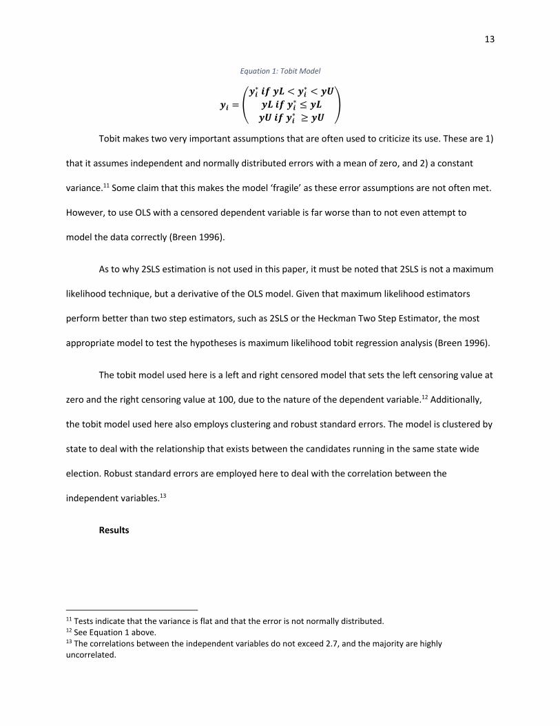
The equation for the tobit model is displayed in Equation 1 below (Breen 1996).10

8 An OLS model was estimated without the censored observations and the results were not significantly different from the regular OLS model. This does not however, justify disregarding the possibility of biased coefficients. 9 In the data the NO group was a large segment, further justifying tobit regression. 10 The latent variable formulation of the tobit model equation is included in the appendix.

13

Equation 1: Tobit Model

𝒚𝒊 = (

𝒚𝒊∗ 𝒊𝒇 𝒚𝑳 < 𝒚𝒊

∗ < 𝒚𝑼

𝒚𝑳 𝒊𝒇 𝒚𝒊∗ ≤ 𝒚𝑳

𝒚𝑼 𝒊𝒇 𝒚𝒊∗ ≥ 𝒚𝑼

)

Tobit makes two very important assumptions that are often used to criticize its use. These are 1)

that it assumes independent and normally distributed errors with a mean of zero, and 2) a constant

variance.11 Some claim that this makes the model ‘fragile’ as these error assumptions are not often met.

However, to use OLS with a censored dependent variable is far worse than to not even attempt to

model the data correctly (Breen 1996).

As to why 2SLS estimation is not used in this paper, it must be noted that 2SLS is not a maximum

likelihood technique, but a derivative of the OLS model. Given that maximum likelihood estimators

perform better than two step estimators, such as 2SLS or the Heckman Two Step Estimator, the most

appropriate model to test the hypotheses is maximum likelihood tobit regression analysis (Breen 1996).

The tobit model used here is a left and right censored model that sets the left censoring value at

zero and the right censoring value at 100, due to the nature of the dependent variable.12 Additionally,

the tobit model used here also employs clustering and robust standard errors. The model is clustered by

state to deal with the relationship that exists between the candidates running in the same state wide

election. Robust standard errors are employed here to deal with the correlation between the

independent variables.13

Results

11 Tests indicate that the variance is flat and that the error is not normally distributed. 12 See Equation 1 above. 13 The correlations between the independent variables do not exceed 2.7, and the majority are highly uncorrelated.

14

Looking back at Table 1, it is important to note that the dependent variable ranges from nearly

zero to eighty percent, with a mean of about 3.5 percent. This helps to put the results from the model

into perspective. Thus, it can generally be understood that digital spending is, at least for the mean

Senator, not a large segment of the total campaign budget.

Digging deeper, Table 2 (below) shows that the first hypothesis, regarding the general

effectiveness of various control variables, such as party ID, quality challenger, both competitive

variables, and challenger status are not statistically significant, nor are they substantively significant.

Thus, these tried and true variables from the literature do not assist in explaining digital spending. Thus,

it appears that the first hypothesis can be safely put to rest as not holding true (an exception applies

here and will be discussed shortly).14

Table 2: Model Results

Variable Tobit Model Percent Digital b/se

Population 0.014

(0.05)

Age 0.03 (0.03)

Democrat -0.606 (1.19)

Challenger 0.189 (1.26)

Open Seat 2.052* (1.04)

Gender 0.261 (0.98)

Quality Challenger -1.237 (1.37)

Competitive Primary 8.043 (6.99)

Competitive General -0.085 (0.98)

2010 -0.966 (1.65)

2012 -0.859 (0.96)

2014 . .

Constant 1.238 (2.48)

Sigma . Constant 6.978*

(2.67)

14 The model was estimated separately for the two major political parties, and the results remained consistent.

15

AIC 886.61 BIC 924 N 128

The second hypothesis, regarding the impact of a candidates age on the cost of information and

the relative level of uncertainty surrounding digital spending can be seen as not true. So, age has little to

no impact on a Senator’s ability to employ digital spending, and if they do, it is likely to be a small

percentage. This has implications that are linked to the incumbency prerequisites, and may even

propose an interesting question, about the impact of staff members, who may make up for the

candidates lack of knowledge on new technology (Downs 1985).15

The third hypothesis, which argued that gender may have an impact on digital spending through

the self-selection process (females being more skilled than their male counter parts), does not bear

statistical fruit in the results. Gender is not a significant predictor of the amount of digital spending

selected by a campaign. This seems to indicate that at least when it comes to the selection of where to

advertise, both male and female candidates seems to have similar profiles (Anzi and Berry 2011).16

While the three hypotheses generated in the theory section of this paper do not bear any fruit,

there is one interesting result that can be gleamed from the data. According to Table 2, the open seat

variable is significant at the .05 level. Based on the coefficient value, it can be determined that a one

percent increase in digital spending results in a 2.05 increase in the predicted value of digital spending.

This statistical result is further proof that the work of Abramowitz is correct, the open seat control

variable is vitally important in the campaign spending literature and in other related work such as this

one. This results can be explained via the argument that open seat elections see a larger amount of

15 The model was estimated separately for Senators past the age of mandatory retirement (65) and those who were below this age. The results remained consistent with the results shown. 16 The model was estimated separately for each gender, and the results remained consistent with the ones shown.

16

spending on advertising than races that have an incumbent candidate (Abramowitz 1989; Erikson and

Palfrey 1998; Levitt 1994).

Conclusion

In the previous sections, it was found that the three hypotheses put forth were not

substantiated in the data. With the exception of the open seat variable, which confirms the work of

Abramowitz (1989), the literature derived variables do not perform as expected. Often used variables

such as quality candidate, among others, were not significant. Additionally, the variables that were

theorized to impact digital spending (age and gender) did not perform as theorized.

Thus, despite the rampant speculation by both journalists and scholars that social media and

other forms of digital spending have a high impact is untrue, based on the results of this paper. It

appears that such a claim is at best highly limited. The election of 2008 does not seem to alter the

means used by rational political candidates by much, signified by the fact that the mean percentage of

digital spending is 3.5% of total spending. While it does not appear to have a large impact in the election

cycles immediately preceding 2008, there is an argument to be made that a possible learning curve may

exist for political campaigns. Thus, these null results should be interpreted with skepticism and tested

again when more data is available.

However, the merits of work such as this, and others (van Heerde, Johnson, and Bowler 2006)

do seem to indicate that disaggregating advertising into its components is a fruitful line of scholarship.

Given the results from this paper, future work could investigate the other more important forms of

spending such as, media or canvassing. Given the small mean for digital spending, the question remains,

what other forms of spending make up larger percentages, and how do they vary given candidate

preferences, characteristics, information costs, and uncertainty.

17

This work does however contribute a valuable theoretical point. The typical causal chain used in

the campaign spending literature is inaccurate and needs to be revised. This paper argues for a similar

approach to the work of Ansolabhere, Figueiredo, and Snyder (2003), in that advertising needs to be

viewed as a strategic choice of rational political actors on where to allocate funds. While it may be

tempting to model votes similar to others in the literature (Jacobson 78; Jacobson 1981; Jacobson 1990;

Green and Krasno 1988, and others), but this theoretical construction of the causal relationship is

inaccurate from the rational choice perspective, as the ends of a rational actor are beyond the pale

(Downs 1985). The causal chain employed in this work more accurately reflects both the spirit of rational

choice, and also the observed relationship in reality.

18

References

Abramowitz, Alan I. 1989. "Campaign Spending in US Senate Elections." Legislative Studies Quarterly

14:4 487-507 JSTOR.

"About Us." About Us • Instagram. Accessed October 8, 2016. https://www.instagram.com/about/us/.

“About the FEC.” Accessed October 8, 2016. fec.gov/about.shtml

Ansolabehere, Stephen, John M. de Figueiredo, and James M. Snyder. 2003. "Why Is There So Little

Money in U.S. Politics?" The Journal of Economic Perspectives 17:1 105-130 JSTOR.

Anzia, Sarah F., and Christopher R. Berry. "The Jackie (and Jill) Robinson effect: why do congresswomen

outperform congressmen?." American Journal of Political Science 55, no. 3 (2011): 478-493.

Dutta, Soumitra, and Matthew Fraser. "Barack Obama and the Facebook Election." US News. November

19, 2008. Accessed October 18, 2016.

Benoit, Kenneth, and Michael Marsh. 2008. “The Campaign Value of Incumbency: A New Solution to the

Puzzle of Less Effective Incumbent Spending.” American Journal of Political Science. 52:4. 874-

890. JSTOR.

Breen, Richard. ”Regression Models. Quantitative Applications in the Social Sciences.” SAGE

Publications, Inc., 1996.

Coleman, John J., and Paul F. Manna. 2000. “Congressional Campaign Spending and the Quality of

Democracy.” The Journal of Politics. 62:3. 757-789. JSTOR.

Downs, Anthony. An Economic Theory of Democracy. Addison-Wesly. Boston, MA. 1985.

Erikson, Robert S., and Thomas R. Palfrey. "Equilibria in campaign spending games: Theory and data."

American Political Science Review 94, no. 03 (2000): 595-609.

19

-----------, and Thomas R. Palfrey. "Campaign spending and incumbency: An alternative simultaneous

equations approach." The Journal of Politics 60, no. 02 (1998): 355-373.

Mayhew, David R. Congress: The Electoral Connection. 2nd ed. New Haven: Yale University Press, 1974.

Federal Election, Commission. 2015. Candidate Disbursements. Accessed October 1, 2015.

http://www.fec.gov/data/CandidateDisbursement.do.

"Facebook: About." Accessed September 8, 2016.

https://www.facebook.com/pg/facebook/about/?ref=page_internal.

Franz, Michael, Paul Freedman, Ken Goldstein, and Travis Ridout. 2008. "Understanding the Effect of

Political Advertising on Voter Turnout: A Response to Krasno and Green." The Journal of Politics

70:1 262-268.

Gerber, Alan. 1998. “Estimating the Effect of Campaign Spending on Senate Election Outcomes Using

Instrumental Variables.” The American Political Science Review. 92:2. 401-411. JSTOR.

Grier, Kevin. Campaign Spending and Senate Elections, 1978-1984. Public Choice. Vol. 63. No. 3. (1989).

Pp. 201-219. JSTOR. Accessed Feb, 12 2016.

Goldstein, Ken, and Paul Freedman. 2000. "New Evidence for New Arguments: Money and Advertising in

the 1996 Senate Elections." The Journal of Politics 62:4 1087-1108 JSTOR.

Hollander, Barry A. "The Role of Media Use in the Recall Versus Recognition of Political Knowledge."

Journal of Broadcasting & Electronic Media 58, no. 1 (2014): 97-113.

Carr, David. "How Obama Tapped Into Social Networks’ Power." The New York Times. November 09,

2008. Accessed October 11, 2016.

20

Jacobson, Gary. Incumbents’ Advantages in the 1978 U.S. Congressional Elections. Legislative Studies

Quarterly. Vol. 6 No. 2 (May 1981). pp. 183-200. JSOTR. Accessed Feb. 12, 2016.

----------. 1978. "The Effects of Campaign Spending in Congressional Election." The American Political

Science Review 72:2 469-491 JSTOR.

-----------. The Effects of Campaign Spending in House Elections: New Evidence for Old Arguments.

American Journal of Political Science. Vol. 34. No. 2. (May 1990) pp. 334-362. JSTOR. Accessed

Feb, 12 2016.

-----------. 1985. "Money and Votes Reconsidered: Congressional Elections 1972-1982." Public Choice

47:1 7-62 JSTOR.

Kaid, Lynda, Juliana Fernandes, and David Painter. 2011. "Effects of Political Advertising in the 2008

Presidential Campaign." American Behavioral Scientist 55:4 437-456.

Kaid, Lynda, Monica Postelnicue, Kristen Landerville, Hyun Yun, and Abby LaGrange. 2007. "The Effects

of Political Advertising on Young Voters ." American Behavioral Scientist 50:9 1137-1151.

Kazee, Thomas A. "The Impact of Electoral Reform: "Open Elections" and the Louisiana Party System."

Publius 13, no. 1 (1983): 131-39. http://www.jstor.org/stable/3330075.

Kenny, Christopher, and Michael McBurnett. 1992. “A Dynamic Model of the Effect of Campaign

Spending on Congressional Vote Choice.” American Journal of Political Science. 36:4. 923-937.

JSTOR.

Krasno, Jonathan, and Donald Green. 2008. "Do Televised Presidential Ads Increase Voter Turnout?

Evidence from a Natural Experiment." The Journal of Politics 70:1 245-261.

21

Kushin, Matthew James, and Masahiro Yamamoto. "Did social media really matter? College students'

use of online media and political decision making in the 2008 election." Mass Communication

and Society 13, no. 5 (2010): 608-630.

Kuzenski, John C. "The Four. Yes, Four. Types of State Primaries." PS: Political Science and Politics 30, no.

2 (1997): 207-08.

Levitt, Steven D., 1994. “Using Repeat Challengers to Estimate the Effect of Campaign Spending on

Election Outcomes in the U.S. House.” Journal of Political Economy. 102:4. 777-798. JSTOR.

Lott, John R. Jr. 2000. “A Simple Explanation for Why Campaign Expenditures Are Increasing: The

Government Is Getting Bigger.” The Journal of Law and Economics. 43:2. 359-394. JSTOR.

Moon, Woojin. 2006. "The Paradox of Less Effective Incumbent Spending: Theory and Tests." British

Journal of Political Science 36:4 705-721 JSTOR.

"Obama Wins the 2008 Presidential Election - in Social Media - Elixir Interactive." Elixir Interactive.

October 04, 2008. Accessed September 18, 2016. http://elixirinteractive.org/obama-wins-2008-

presidential-election-social-media/.

Pfau, Michael, David Park, Lance Holbert, and Jaeho Cho. 2001. "The Effects of Party- and PAC-

Sponsored Issue Advertising and the Potential of Inoculation to Combat Its Impact on the

Democratic Process." American Behavioral Scientist 44:12 2379-2397.

Shen, Fuyuan, Frank Dardis, and Heidi Edwards. 2011. "Advertising Exposure and Message Type:

Exploring the Perceived Effects of Soft-Money Television Political Ads." Journal of Political

Marketing 10:3 215-229.

Shepard, Lawrence. "Does campaign spending really matter?." Public Opinion Quarterly 41, no. 2 (1977):

196-205.

22

Smith, Aaron. "The Internet's Role in Campaign 2008." Pew Research Center: Internet, Science & Tech.

April 15, 2009. Accessed October 18, 2016. http://www.pewinternet.org/2009/04/15/the-

internets-role-in-campaign-2008/.

Stewart III, Charles, and Mark Reynolds. "Television markets and US Senate elections." Legislative

Studies Quarterly (1990): 495-523.

Stratmann, Thomas. "Some talk: Money in politics. A (partial) review of the literature." In Policy

Challenges and Political Responses, pp. 135-156. Springer US, 2005.

----------, Thomas. 2009. "How prices matter in politics: the return to campaign advertising." Public

Choice 140:3 357-377 JSTOR.

Thomas, Scott J., 1989. “Do Incumbent Campaign Expenditures Matter?.” The Journal of Politics. 51:4.

965-976. JSTOR.

"Company | About - Twitter About." Accessed September 8, 2016. https://about.twitter.com/company.

Van Heerde, Jennifer, Martin Johnson, and Shaun Bowler. "Barriers to participation, voter sophistication

and candidate spending choices in US Senate elections." British Journal of Political Science 36,

no. 04 (2006): 745-758.

Zaller, John. 1992. The Nature and Origin of Mass Opinion. New York: Cambridge University Press.

23

Methods Appendix

Latent Variable notation of tobit regression model.

𝒚𝒊∗ = 𝑿𝒊

′𝜷 + 𝒖𝒊

𝒖𝒊 ~ 𝑵 (𝟎, 𝝈𝟐)

𝒚𝒊 = 𝒚𝒊∗ 𝒊𝒇 𝒄𝟏 ≤ 𝒚𝒊

∗ ≤ 𝒄𝟐

𝒚𝒊 = 𝒄𝟏 𝒊𝒇 𝒄𝟏 > 𝒚𝒊∗

𝒚𝒊 = 𝒄𝟐 𝒊𝒇 𝒄𝟐 < 𝒚𝒊∗

The probability the latent variable exceeds the threshold (the upper and lower limits)

𝒑𝒓(𝒚𝒊∗ > (𝒎) = 𝒑𝒓(𝒙𝒊

′𝜷 + 𝒖𝒊 > (𝒎)

= 𝒑𝒓(𝒖𝒊 > 𝒄𝒎 − 𝒙𝒊′𝜷)

= 𝟏 − 𝚽 (𝒄𝒎 − 𝒙𝒊

′𝜷

𝝈)

Thus;

𝒚∗ > 𝒄𝟏 = 𝟏 − 𝚽(𝒄𝟏)

𝒚∗ < 𝒄𝟐 = 𝚽

Test of the mean error at zero assumption for tobit regression model

Mean St. Err. 95% Confidence Interval

Error 3.33 .21 2.91 3.75

This test shows that the tobit model does violate the assumption that the mean error is at zero.

Model performance test using the standard deviation of the dependent variable and the sigma value.

. 322 = .102 → 10%

This indicates that the tobit regression model’s predicted values share approximately 10% of their

variance with the dependent variable (digital spending).