Embed Size (px)
Citation preview

Broadcast protocols for wireless sensor networks 85
Broadcast protocols for wireless sensor networks
Ruiqin Zhao, Xiaohong Shen and Xiaomin Zhang
X
Broadcast protocols for wireless sensor networks
Ruiqin Zhao, Xiaohong Shen and Xiaomin Zhang
Northwestern Polytechnical University P.R.China
1. Introduction
Future network is all about an integrated global network based on an open-systems approach. Integrating different types of wireless networks with wireline backbone networks seamlessly and the convergence of voice, multimedia, and data traffic over a single IP-based core network will be the main focus of 4G. With the availability of ultrahigh bandwidth of up to 100 Mbps, multimedia services can be supported efficiently. Ubiquitous computing is enabled with enhanced system mobility and portability support, and location-based services and support of ad hoc networking are expected. Fig. 1 illustrates the networks and components within the future network architecture. It integrates different network topologies and platforms. There are two levels of integration: the first is the integration of heterogeneous wireless networks with varying transmission characteristics such as wireless LAN (Local Area Network), WAN (Wide Area Network), and PAN (Personal Area Network) as well as mobile ad hoc networks; the second level includes the integration of wireless networks and fixed network-backbone infrastructure, the Internet and PSTN (Public Switched Telephone Network). Recent advancement in wireless communications and electronics has enabled the development of low-cost sensor networks. WSN are composed of a large number of sensor nodes that are densely deployed either inside the phenomenon or very close to it. A wireless sensor network can be used in a wide variety of commercial and military applications such as inventory managing, disaster areas monitoring, patient assisting, and target tracking. The wireless sensor node, being a microelectronic device, can only be equipped with a limited power source. The issue of energy-efficient communication in WSN has been attracting attention of many researches during last several years. Broadcasting is a common operation that allows the node in WSN to share its data efficiently among each other. Broadcasting can be used for network discovery to initiate the configuration of the network, to discover multiple routes between a given pair of nodes, and to query for a piece of desired data in a network (N. B. Chang & M. Liu, 2007). In wireless sensor networks, broadcasting can serve as an efficient solution for the sensors to share their local measurements among each other due to the robustness and the effectiveness of the protocol.
5
www.intechopen.com

Smart Wireless Sensor Networks86
Fig. 1. Future network The traditional way of broadcast in WSN is flooding, which is the straightforward and obvious way. When a source node has a packet to broadcast in the network, it sends the packet to all of its neighbors. Then each node that has received the packet for the first time will rebroadcast the packet to its neighborhood, which leads to the participation of all the nodes in broadcasting the packet. Thus, the traditional flooding which also is known as ordinary broadcast mechanism (OBM), results in serious redundancy, collision and contention, and referred to as broadcast storm problem (S Y Ni et al., 1999). The formation of the broadcast storm problem is due to the redundancy of rebroadcast which results in the serious contention and collision. Moreover, the reduction of the redundancy of rebroadcast is also the requirement of energy-saving in WSN. In networks where each node is assumed to have a fixed level of transmission power, less rebroadcasts means less energy consumed with the assumption that the energy needed by receiving is much less than the energy consumed by transmitting. To save as much energy as possible for each node in the network, the broadcast algorithm should make as less nodes as possible participate in the rebroadcast of the broadcasted message (R.Q. Zhao et al.,2007). Therefore, reduction of
rebroadcast redundancy is significant. A satisfying broadcast strategy should be able to reduce the broadcast redundancy effectively, not only for the saving of bandwidth, but also for the saving of energy, as both bandwidth and energy are valuable resources in WSN. While reduction of rebroadcast redundancy is not the only metric for a good broadcast protocol. There is another metric used for evaluating performance of broadcast protocols called reachability, which indicates the coverage rate of a broadcast algorithm. With the aim of solving the broadcast storm problem and maximizing the network life-time, we propose an efficient broadcast algorithm—Maximum Life-time Localized Broadcast (ML2B) for WSN, which possesses the following properties: a) Localized algorithm.
Localized algorithm is distributed algorithm which achieves a desired global objective with simple local behaviors. Each node makes the decision of rebroadcast based on its one-hop local information, e.g. its own position, its one-hop neighbors’ information and energy left in its battery. Distributed design of broadcast routing is required by the essence of WSN. However, many proposed broadcast approaches were not distributed, such as those approaches selecting rebroadcast nodes based on a constructed broadcast tree which could not be maintained by each node using only its own local information. ML2B need not maintain any global topology information, thus resulting in much less overhead in WSN.
b) Energy-saving approach. It is designed with the aim of minimizing energy required per broadcast task and maximizing network life-time. ML2B is not based on constructing a minimum energy tree which may cause much overhead to maintain the tree. It selects rebroadcast nodes by considering the coverage efficiency and the left energy of the node together to maximize life-time of the whole network. Using the rule of less rebroadcasts results less total energy consumed, ML2B cuts down the total energy consumption in broadcast routing by reducing the redundancy of rebroadcast largely which is capable of relieving the broadcast storm problem synchronously.
c) Degree adaptive broadcast strategy. To reduce the redundancy of rebroadcast, nodes with large degree will be selected with higher priority as forward nodes in ML2B. The degree we use in this paper is the number of left neighbors that have not been covered by the former forward node or by the broadcast originator. Therefore, the rebroadcast of nodes with high degree brings high efficiency of the rebroadcast and great reduction of broadcast redundancy.
d) )Fault tolerant algorithm. For the multi-path and fading effects of the wireless channel, or some sensor nodes may fail or be blocked due to physical damage or environmental interference, protocols used in WSN should be robust. This is the reliability or fault tolerance issue. Fault tolerance is the ability to sustain sensor network functionalities without any interruption due to sensor node failures. ML2B uses a self-selection mechanism to choose nodes that will rebroadcast next from nodes that were able to receive the packets without errors.
The remainder of this chapter is organized as follows. Firstly we make a survey of energy efficient broadcast protocols for wireless sensor networks in Sections 2. Secondly we propose an efficient broadcast protocol for WSN in Sections 3 and 4. It optimizes broadcasting by reducing redundant rebroadcasts and balancing the energy consumption among all nodes. Simulation is done in section 5 to verify the proposed mechanism.
www.intechopen.com

Broadcast protocols for wireless sensor networks 87
Fig. 1. Future network The traditional way of broadcast in WSN is flooding, which is the straightforward and obvious way. When a source node has a packet to broadcast in the network, it sends the packet to all of its neighbors. Then each node that has received the packet for the first time will rebroadcast the packet to its neighborhood, which leads to the participation of all the nodes in broadcasting the packet. Thus, the traditional flooding which also is known as ordinary broadcast mechanism (OBM), results in serious redundancy, collision and contention, and referred to as broadcast storm problem (S Y Ni et al., 1999). The formation of the broadcast storm problem is due to the redundancy of rebroadcast which results in the serious contention and collision. Moreover, the reduction of the redundancy of rebroadcast is also the requirement of energy-saving in WSN. In networks where each node is assumed to have a fixed level of transmission power, less rebroadcasts means less energy consumed with the assumption that the energy needed by receiving is much less than the energy consumed by transmitting. To save as much energy as possible for each node in the network, the broadcast algorithm should make as less nodes as possible participate in the rebroadcast of the broadcasted message (R.Q. Zhao et al.,2007). Therefore, reduction of
rebroadcast redundancy is significant. A satisfying broadcast strategy should be able to reduce the broadcast redundancy effectively, not only for the saving of bandwidth, but also for the saving of energy, as both bandwidth and energy are valuable resources in WSN. While reduction of rebroadcast redundancy is not the only metric for a good broadcast protocol. There is another metric used for evaluating performance of broadcast protocols called reachability, which indicates the coverage rate of a broadcast algorithm. With the aim of solving the broadcast storm problem and maximizing the network life-time, we propose an efficient broadcast algorithm—Maximum Life-time Localized Broadcast (ML2B) for WSN, which possesses the following properties: a) Localized algorithm.
Localized algorithm is distributed algorithm which achieves a desired global objective with simple local behaviors. Each node makes the decision of rebroadcast based on its one-hop local information, e.g. its own position, its one-hop neighbors’ information and energy left in its battery. Distributed design of broadcast routing is required by the essence of WSN. However, many proposed broadcast approaches were not distributed, such as those approaches selecting rebroadcast nodes based on a constructed broadcast tree which could not be maintained by each node using only its own local information. ML2B need not maintain any global topology information, thus resulting in much less overhead in WSN.
b) Energy-saving approach. It is designed with the aim of minimizing energy required per broadcast task and maximizing network life-time. ML2B is not based on constructing a minimum energy tree which may cause much overhead to maintain the tree. It selects rebroadcast nodes by considering the coverage efficiency and the left energy of the node together to maximize life-time of the whole network. Using the rule of less rebroadcasts results less total energy consumed, ML2B cuts down the total energy consumption in broadcast routing by reducing the redundancy of rebroadcast largely which is capable of relieving the broadcast storm problem synchronously.
c) Degree adaptive broadcast strategy. To reduce the redundancy of rebroadcast, nodes with large degree will be selected with higher priority as forward nodes in ML2B. The degree we use in this paper is the number of left neighbors that have not been covered by the former forward node or by the broadcast originator. Therefore, the rebroadcast of nodes with high degree brings high efficiency of the rebroadcast and great reduction of broadcast redundancy.
d) )Fault tolerant algorithm. For the multi-path and fading effects of the wireless channel, or some sensor nodes may fail or be blocked due to physical damage or environmental interference, protocols used in WSN should be robust. This is the reliability or fault tolerance issue. Fault tolerance is the ability to sustain sensor network functionalities without any interruption due to sensor node failures. ML2B uses a self-selection mechanism to choose nodes that will rebroadcast next from nodes that were able to receive the packets without errors.
The remainder of this chapter is organized as follows. Firstly we make a survey of energy efficient broadcast protocols for wireless sensor networks in Sections 2. Secondly we propose an efficient broadcast protocol for WSN in Sections 3 and 4. It optimizes broadcasting by reducing redundant rebroadcasts and balancing the energy consumption among all nodes. Simulation is done in section 5 to verify the proposed mechanism.
www.intechopen.com

Smart Wireless Sensor Networks88
Simulation results show that the proposed broadcast protocol can prolong the network life-time of WSN effectively. Finally, in Section 6 we draw the main conclusions.
2. Related Works
The straightforward way of broadcast is flooding. The advantage of flooding is its simplicity and reliability. However,for its large amount of redundant rebroadcast, flooding will
cause serious packets collision, bandwidth waste,and battery energy exhaustion, which are referred to as broadcast storm problem (S Y Ni et al., 1999). Various approaches have been proposed to solve the broadcast storm problem of flooding for wireless multi-hop networks. Some methods are designed with the aim of alleviating the broadcast storm problem by reducing redundant broadcasts. As in (J. Wu & F. Dai, 2004) ; (M. T. Sun &T. H. Lai, 2002); ( W. Peng & X. C. Lu, 2000), each node computes a local cover set consisting of as less neighbors as possible to cover its whole 2-hop coverage area by exchanging connectivity information with neighbors. These methods require each node know its k-hop (k >=2) neighbor information. To maintain the fresh k-hop (k >=2) neighbor information, these broadcast methods result in heavy overhead on WSN, and they consume much energy at each node. Some methods (S Y Ni et al., 1999); (M. Lin et al., 1999) select forward node based on probability, which cannot guarantee the reachability of the broadcast. Many proposed energy-saving broadcast methods are centralized, which require the topology information of the whole network. They try to find a broadcast tree such that the energy cost of the broadcast tree is minimized. Some methods(J.E. Wieselthier et al., 2000); (P.J. Wan et al., 2001); (M. Cagalj et al., 2002); ( D. Li et al., 2004) are based on geometry or graph information of the network to compute the minimum energy tree. Since the centralized method will cause much overhead in wireless sensor network, some localized versions of the above algorithms have been proposed recently. The algorithm in (M. Agarwal et al., 2004) reduces energy consumption by taking advantage of the physical layer design. (W.Z. Song et al., 2006) proposed a scheme for each node to find the network topology in a distributed way. However the algorithm proposed in (W.Z. Song et al., 2006), also requires each node to maintain the network topology, and the overhead is obviously more than a localized algorithm. The method proposed in (F. Ingelrest & D. Simplot-Ryl., 2005) requires that each node must be aware of the geometry information within its 2-hop neighborhood. It results in more control overhead and energy cost than the thorough distributed algorithm that requires only local one-hop information. Two types of broadcasting protocols(J.-P. Sheu g et al., 2006) are proposed for wireless sensor networks. The two broadcasting protocols, are called one-to-all and all-to-all broadcasting protocols. And the protocols are proposed for five fixed and regular WSN topologies. An energy-saving broadcast method using cooperative transmission in WSN is proposed in (Y.-W. Hong & A. Scaglione, 2006). The cooperation is provided through a system called the Opportunistic Large Array (OLA) where network broadcasting is done through signal processing techniques at the physical layer. In (X. Hui et al., 2006), the practical models for power aware broadcast in wireless ad hoc and sensor networks are analyzed. Some literatures deal with the query execution in large sensor networks, e.g. (J.-P. Sheu et al., 2007); (C. R. Mann et al., 2007). These proposed protocols are designed to
facilitate any type queries for data content and services over a specific geographic region in large population, high-density wireless sensor networks. Several robust data delivery protocols (F. Ye et al., 2005); (Miklós Maróti, 2004) have been proposed for large sensor networks to disseminate data to interested sensors. GRAdient Broadcast (F. Ye et al., 2005) addresses the problem of robust data forwarding to a data collecting unit using unreliable sensor nodes with error-prone wireless channels. A Broadcast Protocol for Sensor networks (BPS) is proposed in (A. Durres i&V. Paruchuri, 2007). BPS uses the location of each node to broadcast packets in a distributed way.
3. System Model
The WSN can be abstracted as a graph ( , )G V E , in whichV is the set of all the nodes in the network and E consists of edges presented in the graph. An edge ( , )e u v , e E exists if the Euclidean distance between node u and v is smaller than r , where r is the radius of the coverage of nodes. We assume all links in the graph is bidirectional, and the graph is in a connected state. Given a node i , time t is recorded since it receives the broadcasted message for the first time, and 0t . The energy left in battery of node i is represented by ( , )e i t . ( , )l i t is defined as the Euclidean distance between node i and the up-link forward node ( , )uf i t which sends the broadcasted message. We assume each node knows its own position information by means of GPS or other instruments. Each node also obtains its one-hop neighbors’ information which is available in most location-aided routing ( F. Ingelrest & D. Simplot-Ryl, 2005) of the ad hoc or sensor networks. Energy left in battery also needs to be provided at every node locally. For i V , several variables are defined as follows: Neighbor ( )nb i , is the node that can communicate directly with node i . It is the one-
hop neighbor of node i . Neighbor set ( )NB i , is the set of all neighbors of node i . Uncovered set ( , )UC i t , consists of one-hop neighbors that have not been covered by a
certain forward node of the broadcasted message or the broadcast originator, before t . Degree ( , )d i t , is the number of nodes belonging to ( , )UC i t at t . ( , )d i t implies the
rebroadcast efficiency of node i . If ( , )d i t is below a threshold before its attempt to rebroadcast the broadcasted message, node i could abandon the attempt.
Up-link forward node ( , )uf i t , is the ( )nb i that rebroadcasts or broadcasts the message which is received by node i at t (0 ( ))t D i . Before ( )t D i , node imay receive several copies of the same broadcasted message from different up-link forward nodes( ( )D i is the add delay of node i ).
Down-link forward node ( , )df i t , is the ( )nb i that rebroadcasts the message at t ( ( ))t D i , after it has received the message from node i . If node i has not rebroadcasted the message at ( )t D i , it will not have any down-link forward node. That is to say, only the forward node has down-link forward node, though except for broadcast originator node each node owns up-link forward node.
www.intechopen.com

Broadcast protocols for wireless sensor networks 89
Simulation results show that the proposed broadcast protocol can prolong the network life-time of WSN effectively. Finally, in Section 6 we draw the main conclusions.
2. Related Works
The straightforward way of broadcast is flooding. The advantage of flooding is its simplicity and reliability. However,for its large amount of redundant rebroadcast, flooding will
cause serious packets collision, bandwidth waste,and battery energy exhaustion, which are referred to as broadcast storm problem (S Y Ni et al., 1999). Various approaches have been proposed to solve the broadcast storm problem of flooding for wireless multi-hop networks. Some methods are designed with the aim of alleviating the broadcast storm problem by reducing redundant broadcasts. As in (J. Wu & F. Dai, 2004) ; (M. T. Sun &T. H. Lai, 2002); ( W. Peng & X. C. Lu, 2000), each node computes a local cover set consisting of as less neighbors as possible to cover its whole 2-hop coverage area by exchanging connectivity information with neighbors. These methods require each node know its k-hop (k >=2) neighbor information. To maintain the fresh k-hop (k >=2) neighbor information, these broadcast methods result in heavy overhead on WSN, and they consume much energy at each node. Some methods (S Y Ni et al., 1999); (M. Lin et al., 1999) select forward node based on probability, which cannot guarantee the reachability of the broadcast. Many proposed energy-saving broadcast methods are centralized, which require the topology information of the whole network. They try to find a broadcast tree such that the energy cost of the broadcast tree is minimized. Some methods(J.E. Wieselthier et al., 2000); (P.J. Wan et al., 2001); (M. Cagalj et al., 2002); ( D. Li et al., 2004) are based on geometry or graph information of the network to compute the minimum energy tree. Since the centralized method will cause much overhead in wireless sensor network, some localized versions of the above algorithms have been proposed recently. The algorithm in (M. Agarwal et al., 2004) reduces energy consumption by taking advantage of the physical layer design. (W.Z. Song et al., 2006) proposed a scheme for each node to find the network topology in a distributed way. However the algorithm proposed in (W.Z. Song et al., 2006), also requires each node to maintain the network topology, and the overhead is obviously more than a localized algorithm. The method proposed in (F. Ingelrest & D. Simplot-Ryl., 2005) requires that each node must be aware of the geometry information within its 2-hop neighborhood. It results in more control overhead and energy cost than the thorough distributed algorithm that requires only local one-hop information. Two types of broadcasting protocols(J.-P. Sheu g et al., 2006) are proposed for wireless sensor networks. The two broadcasting protocols, are called one-to-all and all-to-all broadcasting protocols. And the protocols are proposed for five fixed and regular WSN topologies. An energy-saving broadcast method using cooperative transmission in WSN is proposed in (Y.-W. Hong & A. Scaglione, 2006). The cooperation is provided through a system called the Opportunistic Large Array (OLA) where network broadcasting is done through signal processing techniques at the physical layer. In (X. Hui et al., 2006), the practical models for power aware broadcast in wireless ad hoc and sensor networks are analyzed. Some literatures deal with the query execution in large sensor networks, e.g. (J.-P. Sheu et al., 2007); (C. R. Mann et al., 2007). These proposed protocols are designed to
facilitate any type queries for data content and services over a specific geographic region in large population, high-density wireless sensor networks. Several robust data delivery protocols (F. Ye et al., 2005); (Miklós Maróti, 2004) have been proposed for large sensor networks to disseminate data to interested sensors. GRAdient Broadcast (F. Ye et al., 2005) addresses the problem of robust data forwarding to a data collecting unit using unreliable sensor nodes with error-prone wireless channels. A Broadcast Protocol for Sensor networks (BPS) is proposed in (A. Durres i&V. Paruchuri, 2007). BPS uses the location of each node to broadcast packets in a distributed way.
3. System Model
The WSN can be abstracted as a graph ( , )G V E , in whichV is the set of all the nodes in the network and E consists of edges presented in the graph. An edge ( , )e u v , e E exists if the Euclidean distance between node u and v is smaller than r , where r is the radius of the coverage of nodes. We assume all links in the graph is bidirectional, and the graph is in a connected state. Given a node i , time t is recorded since it receives the broadcasted message for the first time, and 0t . The energy left in battery of node i is represented by ( , )e i t . ( , )l i t is defined as the Euclidean distance between node i and the up-link forward node ( , )uf i t which sends the broadcasted message. We assume each node knows its own position information by means of GPS or other instruments. Each node also obtains its one-hop neighbors’ information which is available in most location-aided routing ( F. Ingelrest & D. Simplot-Ryl, 2005) of the ad hoc or sensor networks. Energy left in battery also needs to be provided at every node locally. For i V , several variables are defined as follows: Neighbor ( )nb i , is the node that can communicate directly with node i . It is the one-
hop neighbor of node i . Neighbor set ( )NB i , is the set of all neighbors of node i . Uncovered set ( , )UC i t , consists of one-hop neighbors that have not been covered by a
certain forward node of the broadcasted message or the broadcast originator, before t . Degree ( , )d i t , is the number of nodes belonging to ( , )UC i t at t . ( , )d i t implies the
rebroadcast efficiency of node i . If ( , )d i t is below a threshold before its attempt to rebroadcast the broadcasted message, node i could abandon the attempt.
Up-link forward node ( , )uf i t , is the ( )nb i that rebroadcasts or broadcasts the message which is received by node i at t (0 ( ))t D i . Before ( )t D i , node imay receive several copies of the same broadcasted message from different up-link forward nodes( ( )D i is the add delay of node i ).
Down-link forward node ( , )df i t , is the ( )nb i that rebroadcasts the message at t ( ( ))t D i , after it has received the message from node i . If node i has not rebroadcasted the message at ( )t D i , it will not have any down-link forward node. That is to say, only the forward node has down-link forward node, though except for broadcast originator node each node owns up-link forward node.
www.intechopen.com

Smart Wireless Sensor Networks90
Up-link forward set ( , )UF i t , is the set of all up-link forward nodes of node i before t . If it has received the same broadcasted message for k times before t ( ( ))t D i , its up-link forward set can be expressed as:
0 1 2 1( , ) ( , ), ( , ), ( , ).... ( , )kUF i t uf i t uf i t uf i t uf i t , ( 1)k (1)
(where 0 1 2, , ...t t t ,and 1kt 1( )kt t records the time node i received the 1st, 2nd, 3rd …, and k th copy of the same broadcasted message).
Down-link forward set ( , )DF i t , consists of all down-link forward nodes of node i before t . Nodes that have not been selected as forward node have an empty down-link forward set. While the down-link forward set of forward
node iwith'k down-link forward nodes is given as follows:
'
'
'
0 1 2 1( , ), ( , ), ( , ).... ( , ) , 1, 0( , ) kdf i t df i t df i t df i t kkDF i t
(2)
(where ' 0k means no rebroadcast is initiated by the rebroadcast of node i ).
4. Maximum Life-time Localized Broadcast (ML2B) Algorithm
4.1 Design for Add-Delay ( )D i Utilization of add-delay in broadcast protocols is to reduce the redundancy of nodes’ rebroadcast and energy consumption. When node i receives a broadcasted message for the first time, it will not rebroadcast it as OBM. It delays a period of add-delay ( )D i before its attempt to do the rebroadcast. Even when ( )D i expires, the node will not rebroadcast it urgently until the node degree ( , ( ))d i D i is larger than the abandoning threshold n . During the period time of 0 ( )t D i , node i could abandon its attempt to rebroadcast the message as soon as its node degree ( , )d i t is equal to or below the threshold, thus reducing the rebroadcast redundancy and energy consumption largely. Nodes with larger add-delay have a higher probability of receiving multiple copies of a certain broadcasted message, before their attempt to rebroadcast. Each reception of the same message decreases the node degree, thus making nodes with large add-delay rebroadcast the message with little probability. While nodes with little add-delay may rebroadcast the message quickly. We assign little add-delay or no-delay to nodes with high rebroadcast efficiency and enough left energy, large add-delay to nodes with large rebroadcast redundancy. To formulate the rebroadcast efficiency, two metrics are presented as follows:
( ,0)( ) , (0 ( ) 1)d da d if i f i
a (3)
( ,0)( ) , (0 ( ) 1)l lr l if i f ir
(4)
Formula (3) is the node degree metric, and formula (4) is the distance metric. a is the maximum node degree, r is the radius of nodes’ coverage. It can be induced from the two formulas that less ( )lf i or ( )df i results in higher rebroadcast efficiency. To maximize the network life-time, we present the third metric----energy metric for selecting proper rebroadcast nodes. If the left energy at a node is smaller than an energy threshold, it refuses to forward the broadcasted message. Otherwise, the node calculates the add-delay based on formula (5) where E is the maximum energy when battery is full, and TE is the energy threshold which is used to prevent nodes with little energy from dying. The selection of TE ’s value affects the performance of ML2B. Too large value will bring low redundancy, but may result in low reachability simultaneously. Too small value, on the other hand, could not prevent the premature crash of nodes with less energy left which may affect the connectivity of WSN. Hence, there is tradeoff in the selection of TE ’s value.
( ,0)( ) , ( ( ,0) )e TT
E e if i E e i EE E
(5)
ML2B first introduces a new metrics for the selection of rebroadcast node in WSN. It incorporates the three metrics presented above together to select rebroadcast nodes with goals of obtaining low rebroadcast redundancy, high reachability, limited latency, and maximized network life-time. We propose two different ways to combine node degree, coverage rate and left energy metrics into a single synthetic metric, based on the product and sum of the three metrics, respectively. If the product is used, then synthetic metric of delaying the attempt to rebroadcast the broadcasted message is given by formula (6). The sum, on the other hand, leads to a new metric shown by formula (7) by suitably selected values of the three factors: , and .
( ( ,0), ( ,0), ( ,0)) ( ) ( ) ( )prod l ef d i l i e i f i f i f i (6)
( ( ,0), ( ,0), ( ,0)) ( ) ( ) ( )sum
d l ef d i l i e i f i f i f i (7) Nodes with minimized ( ( ,0), ( ,0), ( ,0))f d i l i e i , rebroadcast the message with the least latency. We compute the add-delay with the following formula:
( ) . ( ( ,0), ( ,0), ( ,0))D i D f d i l i e i (8) (where D defines the maximum add-delay, ( ( ,0), ( ,0), ( ,0))f d i l i e i is the synthetic metric shown by formula (6) or (7) ). Hence, based on formulas: (3)(8), we can get product and sum versions of add-delay are:
www.intechopen.com

Broadcast protocols for wireless sensor networks 91
Up-link forward set ( , )UF i t , is the set of all up-link forward nodes of node i before t . If it has received the same broadcasted message for k times before t ( ( ))t D i , its up-link forward set can be expressed as:
0 1 2 1( , ) ( , ), ( , ), ( , ).... ( , )kUF i t uf i t uf i t uf i t uf i t , ( 1)k (1)
(where 0 1 2, , ...t t t ,and 1kt 1( )kt t records the time node i received the 1st, 2nd, 3rd …, and k th copy of the same broadcasted message).
Down-link forward set ( , )DF i t , consists of all down-link forward nodes of node i before t . Nodes that have not been selected as forward node have an empty down-link forward set. While the down-link forward set of forward
node iwith'k down-link forward nodes is given as follows:
'
'
'
0 1 2 1( , ), ( , ), ( , ).... ( , ) , 1, 0( , ) kdf i t df i t df i t df i t kkDF i t
(2)
(where ' 0k means no rebroadcast is initiated by the rebroadcast of node i ).
4. Maximum Life-time Localized Broadcast (ML2B) Algorithm
4.1 Design for Add-Delay ( )D i Utilization of add-delay in broadcast protocols is to reduce the redundancy of nodes’ rebroadcast and energy consumption. When node i receives a broadcasted message for the first time, it will not rebroadcast it as OBM. It delays a period of add-delay ( )D i before its attempt to do the rebroadcast. Even when ( )D i expires, the node will not rebroadcast it urgently until the node degree ( , ( ))d i D i is larger than the abandoning threshold n . During the period time of 0 ( )t D i , node i could abandon its attempt to rebroadcast the message as soon as its node degree ( , )d i t is equal to or below the threshold, thus reducing the rebroadcast redundancy and energy consumption largely. Nodes with larger add-delay have a higher probability of receiving multiple copies of a certain broadcasted message, before their attempt to rebroadcast. Each reception of the same message decreases the node degree, thus making nodes with large add-delay rebroadcast the message with little probability. While nodes with little add-delay may rebroadcast the message quickly. We assign little add-delay or no-delay to nodes with high rebroadcast efficiency and enough left energy, large add-delay to nodes with large rebroadcast redundancy. To formulate the rebroadcast efficiency, two metrics are presented as follows:
( ,0)( ) , (0 ( ) 1)d da d if i f i
a (3)
( ,0)( ) , (0 ( ) 1)l lr l if i f ir
(4)
Formula (3) is the node degree metric, and formula (4) is the distance metric. a is the maximum node degree, r is the radius of nodes’ coverage. It can be induced from the two formulas that less ( )lf i or ( )df i results in higher rebroadcast efficiency. To maximize the network life-time, we present the third metric----energy metric for selecting proper rebroadcast nodes. If the left energy at a node is smaller than an energy threshold, it refuses to forward the broadcasted message. Otherwise, the node calculates the add-delay based on formula (5) where E is the maximum energy when battery is full, and TE is the energy threshold which is used to prevent nodes with little energy from dying. The selection of TE ’s value affects the performance of ML2B. Too large value will bring low redundancy, but may result in low reachability simultaneously. Too small value, on the other hand, could not prevent the premature crash of nodes with less energy left which may affect the connectivity of WSN. Hence, there is tradeoff in the selection of TE ’s value.
( ,0)( ) , ( ( ,0) )e TT
E e if i E e i EE E
(5)
ML2B first introduces a new metrics for the selection of rebroadcast node in WSN. It incorporates the three metrics presented above together to select rebroadcast nodes with goals of obtaining low rebroadcast redundancy, high reachability, limited latency, and maximized network life-time. We propose two different ways to combine node degree, coverage rate and left energy metrics into a single synthetic metric, based on the product and sum of the three metrics, respectively. If the product is used, then synthetic metric of delaying the attempt to rebroadcast the broadcasted message is given by formula (6). The sum, on the other hand, leads to a new metric shown by formula (7) by suitably selected values of the three factors: , and .
( ( ,0), ( ,0), ( ,0)) ( ) ( ) ( )prod l ef d i l i e i f i f i f i (6)
( ( ,0), ( ,0), ( ,0)) ( ) ( ) ( )sum
d l ef d i l i e i f i f i f i (7) Nodes with minimized ( ( ,0), ( ,0), ( ,0))f d i l i e i , rebroadcast the message with the least latency. We compute the add-delay with the following formula:
( ) . ( ( ,0), ( ,0), ( ,0))D i D f d i l i e i (8) (where D defines the maximum add-delay, ( ( ,0), ( ,0), ( ,0))f d i l i e i is the synthetic metric shown by formula (6) or (7) ). Hence, based on formulas: (3)(8), we can get product and sum versions of add-delay are:
www.intechopen.com

Smart Wireless Sensor Networks92
[ ( ,0)][ ( ,0)][ ( ,0)]( )( )
pro
T
D a d i E e i r l iD iE E ar
(9)
[ ( ,0)] [ ( ,0)] [ ( ,0)]( ) ( )sum
T
a d i r l i E e iD i Da r E E
(10)
4.2 Algorithm Description ML2B is a delay based broadcast protocol, where add-delay ( )D i is synthetically calculated based on the only one-hop local information at each node, thus making it a truly distributed broadcast algorithm. The final important goal of a broadcast routing algorithm is to carry broadcasted messages to each node in network with as less rebroadcast redundancy as possible, satisfied reachability and maximized life-time of network. ML2B is designed with the idea in mind. Let s be the broadcast originator, the algorithm flow for node i V s may be formalized as follows: Step 0: Initialization: 1j , ( )D i D , ( )UF i . Step 1: If node i has received broadcasted message sM , go to step 2; else if 0j , go to
step 7, else the node is idle, and stay in step 1. Step 2: Check the node ID of originator s and the message ID. If sM is a new message,
go to step 3; else, node i has received the message before, then let 1j j , and go to step 4.
Step 3: Let 0t , and the system time begins. Let 0j , where j indicates the times of the repeated i ’s reception of sM . Let
( ,0) ( )UC i NB i (11)
Thus, node degree ( ,0)d i equals the number of all its neighbors. If ( ,0)e i is smaller than an energy threshold TE , node i abandons its attempt to rebroadcast, and go to step 9.
Step 4: Let jt t , and usejtp to mark the previous-hop node of sM .
jtp
transmitted sM at jt . We assume the propagation delay can be omitted. Then we get:
( , )jj tuf i t p (12)
jtp is the j th up-link forward node of node i . Add
jtp to up-link forward set ( )UF i at last.
Step 5: Based on the locally obtained position of ( , )juf i t , node i computes the geographical coverage range of ( , )juf i t which is expressed as ( , )jC i t . Then it updates ( , )jUC i t by deleting nodes that locate in ( , )jC i t from ( , )jUC i t . Based on the updated ( , )jUC i t , node i could find out its degree ( , )jd i t . If ( , )jd i t n , it abandons its attempt to rebroadcast, and go to step 9; else if 0j go to step 7.
Step 6: 0j means node i has received sM for the first time. It calculates its add-delay ( )D i based on three factors: ( ,0)d i , ( ,0)l i and ( ,0)e i . ( ,0)l i equals the Euclidean distance between node i and ( ,0)uf i . ( ,0)d i has been calculated by step 5, and ( ,0)e i can be obtained locally. When we get the value of the three parameters, the add-delay can be obtained using formula (9) or (10).
Step 7: Check the current time t : if ( )t D i , go to step 1; else let ( , ) ( , )jd i t d i t . Step 8: If ( , )jd i t n , node i abandons its attempt to rebroadcast; else rebroadcasts sM to
all its neighbors. Step 9: the algorithm ends. Option for the value of abandoning threshold n affects the rebroadcast redundancy and reachability. There is a tradeoff between the two performance metrics, in which large n leads to low reachability, while little one may not achieve as low broadcast redundancy as large n could achieve. The value of abandoning threshold can be selected depending upon the scenarios and applications of WSN.
5. Performance Evaluation
To verify the proposed ML2B, we made lots of simulations using NS-2 (NS-2, 2006) which is a network simulator supported by DARPA and NSF, with an 802.11 MAC layer. We study the performance of ML2B in the simulated wireless ad hoc networks. Nodes in the wireless multi-hop network are placed randomly in a 2-D square area. For all simulation results, each broadcast stream consists of packets of size 512 bytes and the inter arrival time is uniformly distributed around a mean rate varying from 2 packets-per-second (pps) to 10 pps depending upon the simulation scenarios. In the all simulations made in this paper, we use the formula (10) to calculate the add-delay for each node by selection that ( ) 2 ( ) 2d df i f i . The abandoning threshold and energy threshold used in our simulations are configured as / 5n b and / 100TE E , where b is the average number of neighbors of nodes.
5.1. Performance Metrics Used in Simulations We consider four performance metrics: Saved rebroadcast (SRB): ( ) /x y x , where x is the number of nodes that receive the
broadcasted message, and y is the number of nodes that rebroadcasts the message after their reception of the message.
Reachability (RE): /x z , where z is the number of all nodes in the simulated connected network. So RE is also known as the coverage rate.
Maximum end-to-end delay (MED): the interval form the time the broadcasted message is initiated to the time the last node in the network receiving the message.
Life-time (LT): the interval from the time the network is initiated to the time the first node dies.
The saved rebroadcast (SRB) and reachability (RE) metrics were utilized to evaluate the performance of broadcast algorithms by most of the proposed broadcast approaches (S Y Ni et al., 1999) ; (D. Katsaros &Y. Manolopoulos, 2006) ; ( F. Ingelrest & D. Simplot-Ryl, 2005) etc.
www.intechopen.com

Broadcast protocols for wireless sensor networks 93
[ ( ,0)][ ( ,0)][ ( ,0)]( )( )
pro
T
D a d i E e i r l iD iE E ar
(9)
[ ( ,0)] [ ( ,0)] [ ( ,0)]( ) ( )sum
T
a d i r l i E e iD i Da r E E
(10)
4.2 Algorithm Description ML2B is a delay based broadcast protocol, where add-delay ( )D i is synthetically calculated based on the only one-hop local information at each node, thus making it a truly distributed broadcast algorithm. The final important goal of a broadcast routing algorithm is to carry broadcasted messages to each node in network with as less rebroadcast redundancy as possible, satisfied reachability and maximized life-time of network. ML2B is designed with the idea in mind. Let s be the broadcast originator, the algorithm flow for node i V s may be formalized as follows: Step 0: Initialization: 1j , ( )D i D , ( )UF i . Step 1: If node i has received broadcasted message sM , go to step 2; else if 0j , go to
step 7, else the node is idle, and stay in step 1. Step 2: Check the node ID of originator s and the message ID. If sM is a new message,
go to step 3; else, node i has received the message before, then let 1j j , and go to step 4.
Step 3: Let 0t , and the system time begins. Let 0j , where j indicates the times of the repeated i ’s reception of sM . Let
( ,0) ( )UC i NB i (11)
Thus, node degree ( ,0)d i equals the number of all its neighbors. If ( ,0)e i is smaller than an energy threshold TE , node i abandons its attempt to rebroadcast, and go to step 9.
Step 4: Let jt t , and usejtp to mark the previous-hop node of sM .
jtp
transmitted sM at jt . We assume the propagation delay can be omitted. Then we get:
( , )jj tuf i t p (12)
jtp is the j th up-link forward node of node i . Add
jtp to up-link forward set ( )UF i at last.
Step 5: Based on the locally obtained position of ( , )juf i t , node i computes the geographical coverage range of ( , )juf i t which is expressed as ( , )jC i t . Then it updates ( , )jUC i t by deleting nodes that locate in ( , )jC i t from ( , )jUC i t . Based on the updated ( , )jUC i t , node i could find out its degree ( , )jd i t . If ( , )jd i t n , it abandons its attempt to rebroadcast, and go to step 9; else if 0j go to step 7.
Step 6: 0j means node i has received sM for the first time. It calculates its add-delay ( )D i based on three factors: ( ,0)d i , ( ,0)l i and ( ,0)e i . ( ,0)l i equals the Euclidean distance between node i and ( ,0)uf i . ( ,0)d i has been calculated by step 5, and ( ,0)e i can be obtained locally. When we get the value of the three parameters, the add-delay can be obtained using formula (9) or (10).
Step 7: Check the current time t : if ( )t D i , go to step 1; else let ( , ) ( , )jd i t d i t . Step 8: If ( , )jd i t n , node i abandons its attempt to rebroadcast; else rebroadcasts sM to
all its neighbors. Step 9: the algorithm ends. Option for the value of abandoning threshold n affects the rebroadcast redundancy and reachability. There is a tradeoff between the two performance metrics, in which large n leads to low reachability, while little one may not achieve as low broadcast redundancy as large n could achieve. The value of abandoning threshold can be selected depending upon the scenarios and applications of WSN.
5. Performance Evaluation
To verify the proposed ML2B, we made lots of simulations using NS-2 (NS-2, 2006) which is a network simulator supported by DARPA and NSF, with an 802.11 MAC layer. We study the performance of ML2B in the simulated wireless ad hoc networks. Nodes in the wireless multi-hop network are placed randomly in a 2-D square area. For all simulation results, each broadcast stream consists of packets of size 512 bytes and the inter arrival time is uniformly distributed around a mean rate varying from 2 packets-per-second (pps) to 10 pps depending upon the simulation scenarios. In the all simulations made in this paper, we use the formula (10) to calculate the add-delay for each node by selection that ( ) 2 ( ) 2d df i f i . The abandoning threshold and energy threshold used in our simulations are configured as / 5n b and / 100TE E , where b is the average number of neighbors of nodes.
5.1. Performance Metrics Used in Simulations We consider four performance metrics: Saved rebroadcast (SRB): ( ) /x y x , where x is the number of nodes that receive the
broadcasted message, and y is the number of nodes that rebroadcasts the message after their reception of the message.
Reachability (RE): /x z , where z is the number of all nodes in the simulated connected network. So RE is also known as the coverage rate.
Maximum end-to-end delay (MED): the interval form the time the broadcasted message is initiated to the time the last node in the network receiving the message.
Life-time (LT): the interval from the time the network is initiated to the time the first node dies.
The saved rebroadcast (SRB) and reachability (RE) metrics were utilized to evaluate the performance of broadcast algorithms by most of the proposed broadcast approaches (S Y Ni et al., 1999) ; (D. Katsaros &Y. Manolopoulos, 2006) ; ( F. Ingelrest & D. Simplot-Ryl, 2005) etc.
www.intechopen.com

Smart Wireless Sensor Networks94
5.2. Simulation Results Performance Dependence on the Network Scale To study the performance of ML2B under different network scales, we design four scenarios by placing randomly different number of nodes separately in squares areas of different size, to maintain a same node density under different network scales. The packets generation rate in this experiment is 2 pps. As illustrated in Fig. 2 and Fig. 3, ML2B achieves high saved rebroadcast without sacrificing the reachability and maximum end-to-end delay under varying network size. According to expectation, maximum end-to-end delay increases with the increased network scale. From Fig. 3 we can see that the network with 10 nodes has a higher SRB than other cases. That is because 10 nodes randomly placed in a 300m×300m square may be within a node’s coverage area which is larger than the area of the square (radius of a node’s coverage is 250m). The trend of SRB in the left larger scale networks becomes flat, due to the same node density.
0
0. 1
0. 2
0. 3
0. 4
10 50 100 200net wor k nodes
MED
(ms)
ML2B, D=0. 14ML2B, D=0. 04OBM
Fig. 2. MED dependence on network scale.
00. 20. 40. 60. 8
1
10 50 100 200net wor k nodes
RE &
. SR
B
RE: ML2B, D=0. 14 RE: ML2B, D=0. 04SRB: ML2B, D=0. 14 SRB: ML2B, D=0. 04OBM
Fig. 3. SRB &. RE dependence on network scale Performance Dependence on Node Density We made many experiments to study the ML2B performance dependence on node density. For the reason of limited pages, we give the results of the network consisting of 50 nodes, which is shown by Fig. 4 and Fig. 5. The packets generation rate here is 2 pps. Results illustrated by Fig. 5 shows saved rebroadcast of ML2B fall with the decrease of node density. That is because the theoretical value of the saved rebroadcast depends upon the node density. Large density causes big SRB, and ideal SRB will be zero when the node density is below a certain threshold, which is not the main issue of this paper.
0
0. 1
0. 2
0. 3
0. 4
0. 112 0. 224 0. 448 0. 896squar e si ze ( km̂ 2)
MED
(ms)
ML2B, D=0. 14ML2B, D=0. 04OBM
Fig. 4. MED dependence on node density
00. 20. 40. 60. 8
1
0. 112 0. 224 0. 448 0. 896squar e si ze ( km̂ 2)
RE &
. SR
B
RE: ML2B, D=0. 14 RE: ML2B, D=0. 04SRB: ML2B, D=0. 14 SRB: ML2B, D=0. 04OBM
Fig. 5. SRB &. RE dependence on node density We also compare the performance of ML2B with maximum add-delay 0.14D s and 0.04D s. From Fig. 2Fig. 5 it is clear that the former outbalanced the latter in SRB and RE. And both of them have less MED than the OBM in all circumstances. Therefore, in the following experiments we set 0.14D s. Performance Dependence on Packets Generation Rate
0
0. 1
0. 2
0. 3
0. 4
2 4 6 8 10packet gener at i on r at e( pps)
MED
(ms)
ML2BOBM
Fig. 6. MED dependence on network load We study the influence of network load on network performance by varying the packets generation rate from 2 pps to 10 pps. Simulation results in Fig. 6, Fig. 7 show that increased network load incurs little impact on ML2B, however leads to increased MED in OBM. ML2B
www.intechopen.com

Broadcast protocols for wireless sensor networks 95
5.2. Simulation Results Performance Dependence on the Network Scale To study the performance of ML2B under different network scales, we design four scenarios by placing randomly different number of nodes separately in squares areas of different size, to maintain a same node density under different network scales. The packets generation rate in this experiment is 2 pps. As illustrated in Fig. 2 and Fig. 3, ML2B achieves high saved rebroadcast without sacrificing the reachability and maximum end-to-end delay under varying network size. According to expectation, maximum end-to-end delay increases with the increased network scale. From Fig. 3 we can see that the network with 10 nodes has a higher SRB than other cases. That is because 10 nodes randomly placed in a 300m×300m square may be within a node’s coverage area which is larger than the area of the square (radius of a node’s coverage is 250m). The trend of SRB in the left larger scale networks becomes flat, due to the same node density.
0
0. 1
0. 2
0. 3
0. 4
10 50 100 200net wor k nodes
MED
(ms)
ML2B, D=0. 14ML2B, D=0. 04OBM
Fig. 2. MED dependence on network scale.
00. 20. 40. 60. 8
1
10 50 100 200net wor k nodes
RE &
. SR
B
RE: ML2B, D=0. 14 RE: ML2B, D=0. 04SRB: ML2B, D=0. 14 SRB: ML2B, D=0. 04OBM
Fig. 3. SRB &. RE dependence on network scale Performance Dependence on Node Density We made many experiments to study the ML2B performance dependence on node density. For the reason of limited pages, we give the results of the network consisting of 50 nodes, which is shown by Fig. 4 and Fig. 5. The packets generation rate here is 2 pps. Results illustrated by Fig. 5 shows saved rebroadcast of ML2B fall with the decrease of node density. That is because the theoretical value of the saved rebroadcast depends upon the node density. Large density causes big SRB, and ideal SRB will be zero when the node density is below a certain threshold, which is not the main issue of this paper.
0
0. 1
0. 2
0. 3
0. 4
0. 112 0. 224 0. 448 0. 896squar e si ze ( km̂ 2)
MED
(ms)
ML2B, D=0. 14ML2B, D=0. 04OBM
Fig. 4. MED dependence on node density
00. 20. 40. 60. 8
1
0. 112 0. 224 0. 448 0. 896squar e si ze ( km̂ 2)
RE &
. SR
B
RE: ML2B, D=0. 14 RE: ML2B, D=0. 04SRB: ML2B, D=0. 14 SRB: ML2B, D=0. 04OBM
Fig. 5. SRB &. RE dependence on node density We also compare the performance of ML2B with maximum add-delay 0.14D s and 0.04D s. From Fig. 2Fig. 5 it is clear that the former outbalanced the latter in SRB and RE. And both of them have less MED than the OBM in all circumstances. Therefore, in the following experiments we set 0.14D s. Performance Dependence on Packets Generation Rate
0
0. 1
0. 2
0. 3
0. 4
2 4 6 8 10packet gener at i on r at e( pps)
MED
(ms)
ML2BOBM
Fig. 6. MED dependence on network load We study the influence of network load on network performance by varying the packets generation rate from 2 pps to 10 pps. Simulation results in Fig. 6, Fig. 7 show that increased network load incurs little impact on ML2B, however leads to increased MED in OBM. ML2B
www.intechopen.com

Smart Wireless Sensor Networks96
maintains nearly as high RE as OBM and, simultaneously achieves SRB with a value larger than 80%, which reveals the superiority of ML2B over OBM.
00. 20. 40. 60. 8
1
2 4 6 8 10packet gener at i on r at e( pps)
RE &
. SR
BRE: ML2BSRB: ML2B OBM
Fig. 7. SRB &. RE dependence on network load It can be summarized from the above simulations that, ML2B achieves high saved rebroadcast without sacrificing the reachability and maximum end-to-end delay under all circumstances. It is beyond our expectation that ML2B, which has delayed the rebroadcast for an interval of ( )D i , obtains a smaller maximum broadcast end-to-end delay than OBM that has not delayed rebroadcast. For the different add-delay values for different nodes in ML2B greatly alleviates and avoids the contention and its resulting collision problem that persecutes OBM seriously. In ML2B, nodes rebroadcast the message with less contention for the communication channel, thus making ML2B achieve a smaller maximum end-to-end delay than OBM. In a word, ML2B could effectively relieve the broadcast storm problem. Life-Time Evaluation Fig. 8 shows the network life-time of OBM and ML2B under the same scenario, in which each node’s initial energy is uniformly distributed between 0.5 J (joule) and 1.0 J. The first and last node dies separately at 32.48 s and 33.62 s in OBM. After 33.62 s no node dies due to malfunction of the broadcast caused by the unconnectivity of WSN due to the too much dead nodes. While in ML2B, they happen at 73.05 s and 95.0 s separately. Life-time is defined as the interval from the time WSN was initiated to the time the first node died. Obviously, ML2B has more than doubles the useful network life-time compared with OBM.
0
20
40
60
80
100
0 30 32.9 33.4 60 74.6 79.4 80.9 94 97 100
time (s)
node
s stil
l aliv
e
ML2BOBM
Fig. 8. Number of nodes still alive in the network of 100 nodes
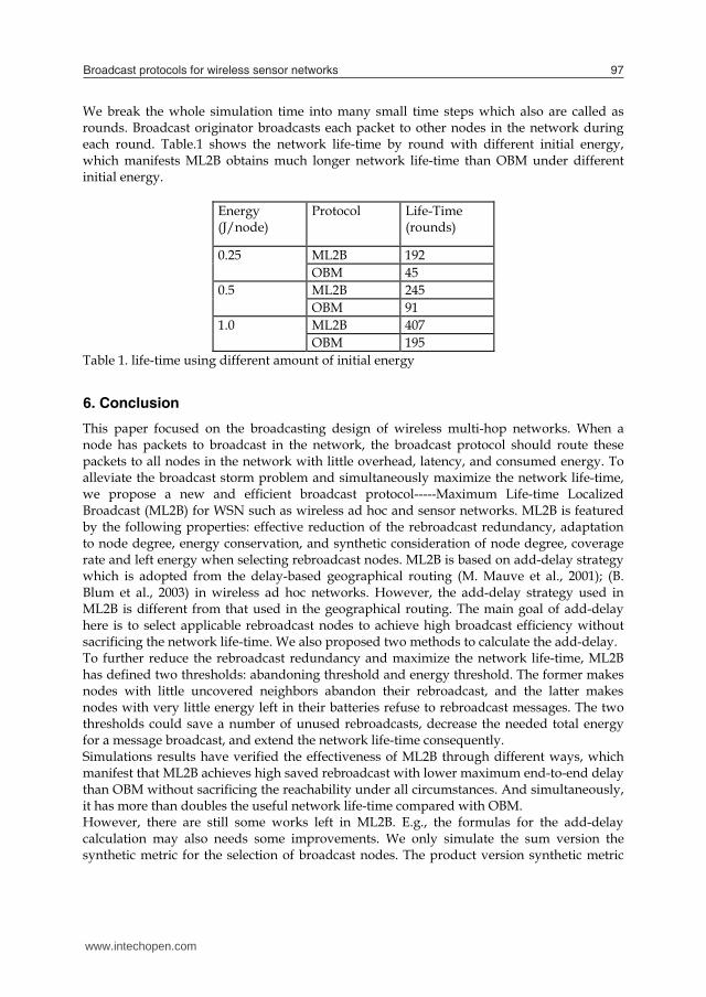
We break the whole simulation time into many small time steps which also are called as rounds. Broadcast originator broadcasts each packet to other nodes in the network during each round. Table.1 shows the network life-time by round with different initial energy, which manifests ML2B obtains much longer network life-time than OBM under different initial energy.
Energy (J/node)
Protocol Life-Time (rounds)
0.25 ML2B 192 OBM 45
0.5 ML2B 245 OBM 91
1.0 ML2B 407 OBM 195
Table 1. life-time using different amount of initial energy
6. Conclusion
This paper focused on the broadcasting design of wireless multi-hop networks. When a node has packets to broadcast in the network, the broadcast protocol should route these packets to all nodes in the network with little overhead, latency, and consumed energy. To alleviate the broadcast storm problem and simultaneously maximize the network life-time, we propose a new and efficient broadcast protocol-----Maximum Life-time Localized Broadcast (ML2B) for WSN such as wireless ad hoc and sensor networks. ML2B is featured by the following properties: effective reduction of the rebroadcast redundancy, adaptation to node degree, energy conservation, and synthetic consideration of node degree, coverage rate and left energy when selecting rebroadcast nodes. ML2B is based on add-delay strategy which is adopted from the delay-based geographical routing (M. Mauve et al., 2001); (B. Blum et al., 2003) in wireless ad hoc networks. However, the add-delay strategy used in ML2B is different from that used in the geographical routing. The main goal of add-delay here is to select applicable rebroadcast nodes to achieve high broadcast efficiency without sacrificing the network life-time. We also proposed two methods to calculate the add-delay. To further reduce the rebroadcast redundancy and maximize the network life-time, ML2B has defined two thresholds: abandoning threshold and energy threshold. The former makes nodes with little uncovered neighbors abandon their rebroadcast, and the latter makes nodes with very little energy left in their batteries refuse to rebroadcast messages. The two thresholds could save a number of unused rebroadcasts, decrease the needed total energy for a message broadcast, and extend the network life-time consequently. Simulations results have verified the effectiveness of ML2B through different ways, which manifest that ML2B achieves high saved rebroadcast with lower maximum end-to-end delay than OBM without sacrificing the reachability under all circumstances. And simultaneously, it has more than doubles the useful network life-time compared with OBM. However, there are still some works left in ML2B. E.g., the formulas for the add-delay calculation may also needs some improvements. We only simulate the sum version the synthetic metric for the selection of broadcast nodes. The product version synthetic metric
www.intechopen.com
Broadcast protocols for wireless sensor networks 97
maintains nearly as high RE as OBM and, simultaneously achieves SRB with a value larger than 80%, which reveals the superiority of ML2B over OBM.
00. 20. 40. 60. 8
1
2 4 6 8 10packet gener at i on r at e( pps)
RE &
. SR
B
RE: ML2BSRB: ML2B OBM
Fig. 7. SRB &. RE dependence on network load It can be summarized from the above simulations that, ML2B achieves high saved rebroadcast without sacrificing the reachability and maximum end-to-end delay under all circumstances. It is beyond our expectation that ML2B, which has delayed the rebroadcast for an interval of ( )D i , obtains a smaller maximum broadcast end-to-end delay than OBM that has not delayed rebroadcast. For the different add-delay values for different nodes in ML2B greatly alleviates and avoids the contention and its resulting collision problem that persecutes OBM seriously. In ML2B, nodes rebroadcast the message with less contention for the communication channel, thus making ML2B achieve a smaller maximum end-to-end delay than OBM. In a word, ML2B could effectively relieve the broadcast storm problem. Life-Time Evaluation Fig. 8 shows the network life-time of OBM and ML2B under the same scenario, in which each node’s initial energy is uniformly distributed between 0.5 J (joule) and 1.0 J. The first and last node dies separately at 32.48 s and 33.62 s in OBM. After 33.62 s no node dies due to malfunction of the broadcast caused by the unconnectivity of WSN due to the too much dead nodes. While in ML2B, they happen at 73.05 s and 95.0 s separately. Life-time is defined as the interval from the time WSN was initiated to the time the first node died. Obviously, ML2B has more than doubles the useful network life-time compared with OBM.
0
20
40
60
80
100
0 30 32.9 33.4 60 74.6 79.4 80.9 94 97 100
time (s)
node
s stil
l aliv
e
ML2BOBM
Fig. 8. Number of nodes still alive in the network of 100 nodes
We break the whole simulation time into many small time steps which also are called as rounds. Broadcast originator broadcasts each packet to other nodes in the network during each round. Table.1 shows the network life-time by round with different initial energy, which manifests ML2B obtains much longer network life-time than OBM under different initial energy.
Energy (J/node)
Protocol Life-Time (rounds)
0.25 ML2B 192 OBM 45
0.5 ML2B 245 OBM 91
1.0 ML2B 407 OBM 195
Table 1. life-time using different amount of initial energy
6. Conclusion
This paper focused on the broadcasting design of wireless multi-hop networks. When a node has packets to broadcast in the network, the broadcast protocol should route these packets to all nodes in the network with little overhead, latency, and consumed energy. To alleviate the broadcast storm problem and simultaneously maximize the network life-time, we propose a new and efficient broadcast protocol-----Maximum Life-time Localized Broadcast (ML2B) for WSN such as wireless ad hoc and sensor networks. ML2B is featured by the following properties: effective reduction of the rebroadcast redundancy, adaptation to node degree, energy conservation, and synthetic consideration of node degree, coverage rate and left energy when selecting rebroadcast nodes. ML2B is based on add-delay strategy which is adopted from the delay-based geographical routing (M. Mauve et al., 2001); (B. Blum et al., 2003) in wireless ad hoc networks. However, the add-delay strategy used in ML2B is different from that used in the geographical routing. The main goal of add-delay here is to select applicable rebroadcast nodes to achieve high broadcast efficiency without sacrificing the network life-time. We also proposed two methods to calculate the add-delay. To further reduce the rebroadcast redundancy and maximize the network life-time, ML2B has defined two thresholds: abandoning threshold and energy threshold. The former makes nodes with little uncovered neighbors abandon their rebroadcast, and the latter makes nodes with very little energy left in their batteries refuse to rebroadcast messages. The two thresholds could save a number of unused rebroadcasts, decrease the needed total energy for a message broadcast, and extend the network life-time consequently. Simulations results have verified the effectiveness of ML2B through different ways, which manifest that ML2B achieves high saved rebroadcast with lower maximum end-to-end delay than OBM without sacrificing the reachability under all circumstances. And simultaneously, it has more than doubles the useful network life-time compared with OBM. However, there are still some works left in ML2B. E.g., the formulas for the add-delay calculation may also needs some improvements. We only simulate the sum version the synthetic metric for the selection of broadcast nodes. The product version synthetic metric
www.intechopen.com

Smart Wireless Sensor Networks98
shown by formula (9) will be investigated and simulated in the future work to evaluate its performances.
7. Acknowledgements
The first author would like to acknowledge helpful discussion and solid support from the co-authors of the chapter. This work was supported by NPU Foundation for Fundamental Research (NPU-FFR-JC201004).
8. References
A. Durresi, V. Paruchuri, “Broadcast protocol for energy-constrained networks,” IEEE Transactions on Broadcasting, vol. 53, no. 1, Mar. 2007, pp. 112-119.
B. Blum, T. He, S. Son, J. Stankovic. IGF: A State-free Robust Communication Protocol for Wireless Sensor Networks. Department of Computer Science, University of Virginia, USA, Tech. Rep. CS-2003-11, 2003.
C. R. Mann, R. O. Baldwin, J. P. Kharoufeh, and B. E. Mullins, “A trajectory-based selective broadcast query protocol for large-scale, high-density wireless sensor networks,” Telecommunication System, vol. 35, no. 1-2, Jun. 2007, pp. 67–86.
D. Li, X. Jia, and H. Liu, “Minimum energy-cost broadcast routing in static ad hoc wireless networks,” IEEE Transactions on Mobile Computing, vol. 3, no. 2, Apr.-Jun. 2004.
F. Ingelrest and D. Simplot-Ryl, “Localized broadcast incremental power protocol for wireless ad hoc networks,” Proc. IEEE ISCC, 2005.
F. Ye, G. Zhong, S. Lu, and L. Zhang, “GRAdient broadcast: a robust data delivery protocol for large scale sensor networks,” Wireless Networks, vol. 11, no. 3, May 2005, pp. 285–298.
J.E. Wieselthier, G.D. Nguyen, and A. Ephremides, “On the construction of energy-efficient broadcast and multicast trees in wireless networks,” Proc. IEEE INFOCOM, 2000.
J.-P. Sheu, C.-S. Hsu and Y.-J. Chang, “Efficient broadcasting protocols for regular wireless sensor networks,” Wireless Communications and Mobile Computing, vol. 6, no. 1, 2006, pp. 35–48.
J.-P. Sheu, S.-C. Tu, and C.-H. Yu, “A distributed query protocol in wireless sensor networks,” Wireless Personal Communications, vol. 41, no.4, Jun. 2007, pp. 449–464.
J. Wu and F. Dai, “A generic distributed broadcast scheme in ad hoc wireless networks,” IEEE Transactions on Computers, vol. 53, no. 10, Oct. 2004, pp. 1343-1354.
M. Agarwal, J. H. Cho, L. Gao, and J. Wu, “Energy efficient broadcast in wireless ad hoc networks with hitch-hiking,” Proc. IEEE INFOCOM, 2004.
M. Cagalj, J.P. Hubaux, and C. Enz, “Minimum-energy broadcast in all-wireless networks: NP-completeness and distribution issues,” Proc. MOBICOM, 2002.
Miklós Maróti, “Directed flood-routing framework for wireless sensor networks,” Proc. IFIP International Federation for Information, LNCS 3231, 2004, pp. 99–114.
M. Lin, K. Marzullo and S. Masini, “Gossip versus deterministic flooding: Low packet overhead and high reliability for broadcasting on small networks.” UCSD Tech. Rep. 0637, 1999.
M. Mauve, J. Widmer, H. Hartenstein. A Survey on Position-Based Routing in Mobile Ad Hoc Networks. IEEE Network. pp. 30-39, Nov. /Dec. 2001.
M.-T. Sun and T.-H. Lai, “Location aided broadcast in wireless ad hoc network systems,” Proc. IEEE WCNC, 2002, pp. 597- 602.
N. B. Chang, and M. Liu, “Controlled flooding search in a large network,” IEEE/ACM Transactions on Networking, vol. 15, no. 2, Apr. 2007, pp. 436-449.
NS-2 Network Simulator , http://isi.edu/nsnam/ns/index.html. Jun. 2009 P.J. Wan, G. Calinescu, X.Y. Li, and O. Frieder, “Minimum-energy broadcast routing in static
ad hoc wireless networks,” Proc. IEEE INFOCOM, 2001. R.Q. Zhao et al., Maximum Life-time Localized Broadcast Routing in MANET. Lecture
Notes in Computer Science, 2007, 4672(1): 193–202. S Y Ni, Y C Tseng, Y S Chen, J P Sheu. The Broadcast Storm problem in a Mobile Ad Hoc
Network. Proceedings of the Fifth Annual ACM/ IEEE International Conference on Mobile Computing and network .Washington: IEEE, pp. 151–162, 1999
W. Peng and X.-C. Lu, “On the reduction of broadcast redundancy in mobile ad hoc networks,” Proc. MOBIHOC, 2000, pp. 129-130.
W.Z. Song, X. Y. Li, and W. Z. Wang, “Localized topology control for unicast and broadcast in wireless ad hoc networks,” IEEE Transactions on Parallel and Distributed Systems, vol. 17, no. 4, 2006, pp. 321-334.
X. Hui, M. Jeon, S. Lei, N. Yu, J. Cho, and S. Lee, “Impact of practical models on power aware broadcast protocols for wireless ad hoc and sensor networks,” Proc. IEEE Workshop on SEUS–CCIA, 2006.
Y.-W. Hong and A. Scaglione, “Energy-Efficient Broadcasting with Cooperative Transmissions in Wireless Sensor Networks,” IEEE Transactions on Wireless Communications, vol. 5, no. 10, Oct. 2006, pp. 2844-2855.
www.intechopen.com

Broadcast protocols for wireless sensor networks 99
shown by formula (9) will be investigated and simulated in the future work to evaluate its performances.
7. Acknowledgements
The first author would like to acknowledge helpful discussion and solid support from the co-authors of the chapter. This work was supported by NPU Foundation for Fundamental Research (NPU-FFR-JC201004).
8. References
A. Durresi, V. Paruchuri, “Broadcast protocol for energy-constrained networks,” IEEE Transactions on Broadcasting, vol. 53, no. 1, Mar. 2007, pp. 112-119.
B. Blum, T. He, S. Son, J. Stankovic. IGF: A State-free Robust Communication Protocol for Wireless Sensor Networks. Department of Computer Science, University of Virginia, USA, Tech. Rep. CS-2003-11, 2003.
C. R. Mann, R. O. Baldwin, J. P. Kharoufeh, and B. E. Mullins, “A trajectory-based selective broadcast query protocol for large-scale, high-density wireless sensor networks,” Telecommunication System, vol. 35, no. 1-2, Jun. 2007, pp. 67–86.
D. Li, X. Jia, and H. Liu, “Minimum energy-cost broadcast routing in static ad hoc wireless networks,” IEEE Transactions on Mobile Computing, vol. 3, no. 2, Apr.-Jun. 2004.
F. Ingelrest and D. Simplot-Ryl, “Localized broadcast incremental power protocol for wireless ad hoc networks,” Proc. IEEE ISCC, 2005.
F. Ye, G. Zhong, S. Lu, and L. Zhang, “GRAdient broadcast: a robust data delivery protocol for large scale sensor networks,” Wireless Networks, vol. 11, no. 3, May 2005, pp. 285–298.
J.E. Wieselthier, G.D. Nguyen, and A. Ephremides, “On the construction of energy-efficient broadcast and multicast trees in wireless networks,” Proc. IEEE INFOCOM, 2000.
J.-P. Sheu, C.-S. Hsu and Y.-J. Chang, “Efficient broadcasting protocols for regular wireless sensor networks,” Wireless Communications and Mobile Computing, vol. 6, no. 1, 2006, pp. 35–48.
J.-P. Sheu, S.-C. Tu, and C.-H. Yu, “A distributed query protocol in wireless sensor networks,” Wireless Personal Communications, vol. 41, no.4, Jun. 2007, pp. 449–464.
J. Wu and F. Dai, “A generic distributed broadcast scheme in ad hoc wireless networks,” IEEE Transactions on Computers, vol. 53, no. 10, Oct. 2004, pp. 1343-1354.
M. Agarwal, J. H. Cho, L. Gao, and J. Wu, “Energy efficient broadcast in wireless ad hoc networks with hitch-hiking,” Proc. IEEE INFOCOM, 2004.
M. Cagalj, J.P. Hubaux, and C. Enz, “Minimum-energy broadcast in all-wireless networks: NP-completeness and distribution issues,” Proc. MOBICOM, 2002.
Miklós Maróti, “Directed flood-routing framework for wireless sensor networks,” Proc. IFIP International Federation for Information, LNCS 3231, 2004, pp. 99–114.
M. Lin, K. Marzullo and S. Masini, “Gossip versus deterministic flooding: Low packet overhead and high reliability for broadcasting on small networks.” UCSD Tech. Rep. 0637, 1999.
M. Mauve, J. Widmer, H. Hartenstein. A Survey on Position-Based Routing in Mobile Ad Hoc Networks. IEEE Network. pp. 30-39, Nov. /Dec. 2001.
M.-T. Sun and T.-H. Lai, “Location aided broadcast in wireless ad hoc network systems,” Proc. IEEE WCNC, 2002, pp. 597- 602.
N. B. Chang, and M. Liu, “Controlled flooding search in a large network,” IEEE/ACM Transactions on Networking, vol. 15, no. 2, Apr. 2007, pp. 436-449.
NS-2 Network Simulator , http://isi.edu/nsnam/ns/index.html. Jun. 2009 P.J. Wan, G. Calinescu, X.Y. Li, and O. Frieder, “Minimum-energy broadcast routing in static
ad hoc wireless networks,” Proc. IEEE INFOCOM, 2001. R.Q. Zhao et al., Maximum Life-time Localized Broadcast Routing in MANET. Lecture
Notes in Computer Science, 2007, 4672(1): 193–202. S Y Ni, Y C Tseng, Y S Chen, J P Sheu. The Broadcast Storm problem in a Mobile Ad Hoc
Network. Proceedings of the Fifth Annual ACM/ IEEE International Conference on Mobile Computing and network .Washington: IEEE, pp. 151–162, 1999
W. Peng and X.-C. Lu, “On the reduction of broadcast redundancy in mobile ad hoc networks,” Proc. MOBIHOC, 2000, pp. 129-130.
W.Z. Song, X. Y. Li, and W. Z. Wang, “Localized topology control for unicast and broadcast in wireless ad hoc networks,” IEEE Transactions on Parallel and Distributed Systems, vol. 17, no. 4, 2006, pp. 321-334.
X. Hui, M. Jeon, S. Lei, N. Yu, J. Cho, and S. Lee, “Impact of practical models on power aware broadcast protocols for wireless ad hoc and sensor networks,” Proc. IEEE Workshop on SEUS–CCIA, 2006.
Y.-W. Hong and A. Scaglione, “Energy-Efficient Broadcasting with Cooperative Transmissions in Wireless Sensor Networks,” IEEE Transactions on Wireless Communications, vol. 5, no. 10, Oct. 2006, pp. 2844-2855.
www.intechopen.com

www.intechopen.com

Smart Wireless Sensor NetworksEdited by Yen Kheng Tan
ISBN 978-953-307-261-6Hard cover, 418 pagesPublisher InTechPublished online 14, December, 2010Published in print edition December, 2010
InTech EuropeUniversity Campus STeP Ri Slavka Krautzeka 83/A 51000 Rijeka, Croatia Phone: +385 (51) 770 447
InTech ChinaUnit 405, Office Block, Hotel Equatorial Shanghai No.65, Yan An Road (West), Shanghai, 200040, China
Phone: +86-21-62489820 Fax: +86-21-62489821
The recent development of communication and sensor technology results in the growth of a new attractive andchallenging area – wireless sensor networks (WSNs). A wireless sensor network which consists of a largenumber of sensor nodes is deployed in environmental fields to serve various applications. Facilitated with theability of wireless communication and intelligent computation, these nodes become smart sensors which do notonly perceive ambient physical parameters but also be able to process information, cooperate with each otherand self-organize into the network. These new features assist the sensor nodes as well as the network tooperate more efficiently in terms of both data acquisition and energy consumption. Special purposes of theapplications require design and operation of WSNs different from conventional networks such as the internet.The network design must take into account of the objectives of specific applications. The nature of deployedenvironment must be considered. The limited of sensor nodes’ resources such as memory, computationalability, communication bandwidth and energy source are the challenges in network design. A smart wirelesssensor network must be able to deal with these constraints as well as to guarantee the connectivity, coverage,reliability and security of network’s operation for a maximized lifetime. This book discusses various aspectsof designing such smart wireless sensor networks. Main topics includes: design methodologies, networkprotocols and algorithms, quality of service management, coverage optimization, time synchronization andsecurity techniques for sensor networks.
How to referenceIn order to correctly reference this scholarly work, feel free to copy and paste the following:
Northwest Polytechnical University Rqzhao and Xiaohong Shen (2010). Broadcast Protocols for WirelessSensor Networks, Smart Wireless Sensor Networks, Yen Kheng Tan (Ed.), ISBN: 978-953-307-261-6, InTech,Available from: http://www.intechopen.com/books/smart-wireless-sensor-networks/broadcast-protocols-for-wireless-sensor-networks
www.intechopen.com

Fax: +385 (51) 686 166www.intechopen.com
Fax: +86-21-62489821

© 2010 The Author(s). Licensee IntechOpen. This chapter is distributedunder the terms of the Creative Commons Attribution-NonCommercial-ShareAlike-3.0 License, which permits use, distribution and reproduction fornon-commercial purposes, provided the original is properly cited andderivative works building on this content are distributed under the samelicense.

![Pseudo geometric broadcast protocols in wireless sensor ... · Performance evaluation Wireless sensor networks a b s t r a c t ... (BPS) [8], de- ... a distributed manner, and it](https://img.dokumen.tips/doc/110x75/5e83f50fe93d207519410593/pseudo-geometric-broadcast-protocols-in-wireless-sensor-performance-evaluation.jpg)