BROADBAND COHERENT LIGHT GENERATION IN RAMAN-ACTIVE

CRYSTALS DRIVEN BY FEMTOSECOND LASER FIELDS

A Dissertation

by

MIAOCHAN ZHI

Submitted to the Office of Graduate Studies ofTexas A&M University

in partial fulfillment of the requirements for the degree of

DOCTOR OF PHILOSOPHY

December 2007

Major Subject: Physics

BROADBAND COHERENT LIGHT GENERATION IN RAMAN-ACTIVE

CRYSTALS DRIVEN BY FEMTOSECOND LASER FIELDS

A Dissertation

by

MIAOCHAN ZHI

Submitted to the Office of Graduate Studies ofTexas A&M University

in partial fulfillment of the requirements for the degree of

DOCTOR OF PHILOSOPHY

Approved by:

Chair of Committee, Alexei V. SokolovCommittee Members, Edward Fry

George KattawarPhilip Hemmer

Head of Department, Edward Fry

December 2007

Major Subject: Physics

iii

ABSTRACT

Broadband Coherent Light Generation in Raman-active

Crystals Driven by Femtosecond Laser Fields. (December 2007)

Miaochan Zhi, B.E., Zhejiang University;

M.S., Zhejiang University

Chair of Advisory Committee: Dr. A. V. Sokolov

I studied a family of closely connected topics related to the production and ap-

plication of ultrashort laser pulses. I achieved broadband cascade Raman generation

in crystals, producing mutually coherent frequency sidebands which can possibly be

used to synthesize optical pulses as short as a fraction of a femtosecond (fs). Un-

like generation using gases, there is no need for a cumbersome vacuum system when

working with room temperature crystals. Our method, therefore, shows promise for

a compact system.

One problem for sideband generation in solids is phase matching, because the

dispersion is significant. I solved this problem by using non-collinear geometry. I

observed what to our knowledge is a record-large number of spectral sidebands gen-

erated in a popular Raman crystal PbWO4 covering infrared, visible, and ultraviolet

spectral regions, when I applied two 50 fs laser pulses tuned close to the Raman

resonance. Similar generation in diamond was also observed, which shows that the

method is universal. When a third probe pulse is applied, a very interesting 2-D color

array is generated in both crystals.

As many as 40 anti-Stokes and 5 Stokes sidebands are generated when a pair of

time-delayed linear chirped pulses are applied to the PbWO4 crystal. This shows that

pulses with picosecond duration, which is on the order of the coherence decay time,

is more effective for sidebands generation than Fourier transform limited fs pulses.

iv

I also studied the technique of fs coherent Raman anti-Stokes scattering (CARS)

which is used as a tool for detecting dipicolinic acid, the marker molecule for bacterial

spores. I observed that there is a maximum when the concentration dependence of

the near-resonant CARS signal is measured. I presented a model to describe this

behavior, and found an analytical solution that agrees with our experimental data.

Theoretically, I explored a possible application for single-cycle pulses: laser in-

duced nuclear fusion. I performed both classical and quantum mechanical calculations

for a system of two nuclei moving under a superintense ultrashort field. From our

calculation I noted that the nuclear collisions occur on a sub-attosecond time scale,

and are predicted to result in an emission of zeptosecond bursts of light.

v

In memory of my parents, Taizhang Zhi and Song’e Wei

vi

ACKNOWLEDGMENTS

First I’d like to thank Dr. Sokolov for giving me the opportunity to carry out this

research, which involves many exciting physics problems. His enthusiasm for research

is inspiring and fosters an atmosphere of discovery. His wealth of knowledge is key in

guiding my research.

I want to particularly thank Dr. Scully. Without his help, I would not have been

admitted as a graduate student here. Later he gave me the opportunity of working

on the fs-CARS project, which eventually lead to the bulk of the research for this

dissertation. Dmitry Pestov, Robert K. Murawski, Xi Wang and Yuri Rostovtsev

are a few of the people who have helped me tremendously during my research. The

happy and exciting days of working with them will remain in my memory forever.

I am grateful to Dr. Hemmer for introducing me to the experimental optics

basic skills. He showed me that some experiments can be done by simple, even used

instruments. He broadened my research by kindly offering me free diamond samples.

Dr. Fry and Dr. Kattawar, as busy as they are, guided me through the first difficult

couple of years here. They talked to me using their valuable time.

I’d like to thank Elena Kuznetsova, Zoe Sariyanni, Changhui Li,Vladmir Sautekov,

Pengwang Zhai, Petr Anisimov, Xudong Xu, Serguei Jerebtsov, Dr. Kolomenskii, Siu

Ah Chin, Anatoly Svidzinsky, Ling Wang and many other fellow graduate students

and friends who helped me during my research. I want to specially thank Tagarathi

V. Nageswar Rao and Spiros Vellas at the TAMU supercomputing group for helping

me parallelize the code.

I am very thankful for my husband Tom and my baby Tiya for giving me peace

of mind while writing this dissertation. Lastly, I’d like to thank my family for their

vii

love and support. My father was my first teacher and my mother taught me love. I

thank my brothers and sisters for their guidance, support and sacrifices.

viii

TABLE OF CONTENTS

CHAPTER Page

I INTRODUCTION . . . . . . . . . . . . . . . . . . . . . . . . . . 1

II BASIC CONCEPTS AND THEORY . . . . . . . . . . . . . . . 9

A. Basic concepts . . . . . . . . . . . . . . . . . . . . . . . . . 9

1. Linear pulse propagation in a dispersive medium . . . 9

a. Pulse broadening . . . . . . . . . . . . . . . . . . 10

b. Effective interaction length . . . . . . . . . . . . . 12

2. Nonlinear pulse propagation . . . . . . . . . . . . . . 13

a. Self focusing and white light generation . . . . . . 13

b. Self phase modulation and cross phase modulation 15

3. Raman scattering . . . . . . . . . . . . . . . . . . . . 16

a. Linear Raman scattering . . . . . . . . . . . . . . 16

b. Stimulated Raman scattering . . . . . . . . . . . 18

4. Ultrashort pulse measurement method—SD FROG . . 21

B. Hamiltonian derivation and sidebands generation . . . . . 23

III BROADBAND COHERENT LIGHT GENERATION IN RAMAN-

ACTIVE CRYSTAL PbWO4∗ . . . . . . . . . . . . . . . . . . . 30

A. Introduction . . . . . . . . . . . . . . . . . . . . . . . . . . 30

B. Experimental setup . . . . . . . . . . . . . . . . . . . . . . 32

C. Broadband coherent light generation in Raman-active

crystals using two-color laser fields . . . . . . . . . . . . . 34

1. Generation by excitation of the strong Raman mode

at 901 cm−1 . . . . . . . . . . . . . . . . . . . . . . . 35

2. Generation by excitation of the Raman mode at

325 cm−1 . . . . . . . . . . . . . . . . . . . . . . . . . 40

D. Broadband coherent light generation in the Raman-

active crystal using three-color laser fields . . . . . . . . . 46

1. Planar configuration . . . . . . . . . . . . . . . . . . . 47

2. Box CARS configuration . . . . . . . . . . . . . . . . 48

E. Study of PbWO4 properties . . . . . . . . . . . . . . . . . 52

1. Coherent CARS decay and quantum beating . . . . . 52

2. UV absorption . . . . . . . . . . . . . . . . . . . . . . 54

ix

CHAPTER Page

3. The interference experiment . . . . . . . . . . . . . . . 55

F. Conclusion . . . . . . . . . . . . . . . . . . . . . . . . . . . 57

IV BROADBAND COHERENT LIGHT GENERATION IN DI-

AMOND USING TWO OR THREE-COLOR FS LASER FIELDS 59

A. Introduction . . . . . . . . . . . . . . . . . . . . . . . . . . 59

B. Broadband coherent light generation in diamond driven

by two-color femtosecond laser field . . . . . . . . . . . . . 61

C. Phase matching calculation . . . . . . . . . . . . . . . . . . 66

D. Coherence between the sidebands . . . . . . . . . . . . . . 71

E. The measurement of the coherence decay time of the

CARS/CSRS signals . . . . . . . . . . . . . . . . . . . . . 72

F. Two dimensional color array generation in diamond

driven by three-color femtosecond laser field . . . . . . . . 74

G. Conclusion . . . . . . . . . . . . . . . . . . . . . . . . . . . 75

V BROADBAND GENERATION IN RAMAN CRYSTAL DRIVEN

BY A PAIR OF TIME-DELAYED LINEARLY CHIRPED

PULSES . . . . . . . . . . . . . . . . . . . . . . . . . . . . . . . 77

A. Introduction . . . . . . . . . . . . . . . . . . . . . . . . . . 77

B. Experimental setup . . . . . . . . . . . . . . . . . . . . . . 78

C. Theory . . . . . . . . . . . . . . . . . . . . . . . . . . . . . 80

1. Chirped pulse characterization . . . . . . . . . . . . . 80

2. Coherence preparation . . . . . . . . . . . . . . . . . . 82

D. Experimental results and discussion . . . . . . . . . . . . . 84

1. Self diffraction and the excitation of the Raman

mode at 191 cm−1 . . . . . . . . . . . . . . . . . . . . 84

2. The excitation of the Raman mode at 325 cm−1 . . . . 86

3. The excitation of the Raman mode at 903 cm−1 . . . . 89

E. Conclusion . . . . . . . . . . . . . . . . . . . . . . . . . . . 90

VI FEMTOSECOND COHERENT ANTI-STOKES RAMAN SCAT-

TERING APPLIED TO THE DETECTION OF BACTER-

IAL ENDOSPORES∗ . . . . . . . . . . . . . . . . . . . . . . . . 93

A. Introduction . . . . . . . . . . . . . . . . . . . . . . . . . . 93

B. Concentration dependence of femtosecond coherent anti-

Stokes Raman scattering in the presence of strong ab-

sorption . . . . . . . . . . . . . . . . . . . . . . . . . . . . 94

x

CHAPTER Page

1. Experimental setup . . . . . . . . . . . . . . . . . . . 94

2. Experimental results and discussion . . . . . . . . . . 96

a. Experimental result with a 2 mm cuvette . . . . . 96

b. Theoretical model . . . . . . . . . . . . . . . . . . 98

c. Experimental result with a 100 µm cuvette . . . . 104

C. CSRS in crystalline DPA . . . . . . . . . . . . . . . . . . . 108

D. Conclusion . . . . . . . . . . . . . . . . . . . . . . . . . . . 110

VII NUMERICAL STUDY OF NUCLEAR COLLISIONS IN-

DUCED BY SINGLE-CYCLE LASER PULSES:

MOLECULAR APPROACH TO FUSION∗ . . . . . . . . . . . . 113

A. Introduction . . . . . . . . . . . . . . . . . . . . . . . . . . 113

B. Classical simulation . . . . . . . . . . . . . . . . . . . . . . 115

1. Linearly polarized laser field . . . . . . . . . . . . . . 116

2. Elliptically polarized laser field . . . . . . . . . . . . . 116

C. Statistical ensemble simulation . . . . . . . . . . . . . . . 118

D. Quantum calculation . . . . . . . . . . . . . . . . . . . . . 121

1. 1-d quantum-mechanical calculation results and com-

parison with classical simulation . . . . . . . . . . . . 124

2. 2-d quantum-mechanical calculation results and com-

parison with classical simulation . . . . . . . . . . . . 130

E. Conclusion . . . . . . . . . . . . . . . . . . . . . . . . . . . 134

VIII SUMMARY . . . . . . . . . . . . . . . . . . . . . . . . . . . . . 136

REFERENCES . . . . . . . . . . . . . . . . . . . . . . . . . . . . . . . . . . . . . . . . . . . . . . . . . . . . . . . . . . . . . . . . 140

APPENDIX A . . . . . . . . . . . . . . . . . . . . . . . . . . . . . . . . . . . 150

APPENDIX B . . . . . . . . . . . . . . . . . . . . . . . . . . . . . . . . . . . 152

VITA . . . . . . . . . . . . . . . . . . . . . . . . . . . . . . . . . . . . . . . . 156

xi

LIST OF TABLES

TABLE Page

I The wavelengths and the angles of the generated sidebands. . . . . . 68

II The minimum internuclear distance (×10−14 m) at the different

laser fields calculated from the different approaches. . . . . . . . . . 128

xii

LIST OF FIGURES

FIGURE Page

1 Nonlinear effects in crystal. (a) The intensity of the pump beams

used are below the threshold of self focusing. The sidebands gener-

ated are nice, round spots. (b) The intensity of the pump beams

used are above the threshold of self focusing, which results in

the deterioration of the generated beams. (c) SPM causes pulse

broadening as the pulse propagates through the crystal. . . . . . . . 14

2 Schematic level diagrams for different processes. (a) anti-Stokes

Raman scattering; (b) Stokes Raman scattering; (c) CARS (d)

CSRS; (e) FWM; (f) FWRM. . . . . . . . . . . . . . . . . . . . . . 20

3 Schematics of the SD FROG. The signal pulse is centered at ap-

proximately the time τ/3 of one input pulse (From D. J. Kane

and R. Trebino, IEEE Journal of Quantum Electronics, Vol. 29,

571 (1993)). . . . . . . . . . . . . . . . . . . . . . . . . . . . . . . . . 22

4 Sidebands generated and instantaneous power density versus time

in PbWO4 crystal. The spectrum and temporal waveform for (a)

z=0, (b) z=44.7 µm, the pulse produced has FWHM of 0.64 fs,

(c) z=100 µm. . . . . . . . . . . . . . . . . . . . . . . . . . . . . . . 29

5 (Top) propagation of the ordinary ray and the extraordinary ray

in scheelite PbWO4, a, b, c are the 3 axes of the crystal. k is the

laser wave vector. θ is the angle between the optical axis c and

the k. (Bottom) the refractive index of the two rays. . . . . . . . . . 31

6 Raman spectrum of the PbWO4 crystal at two different orienta-

tions using a CCD camera (ISA Jobin YVon U1000). The spec-

trometer grating has a groove density of 1800 grooves/mm. This

measurement has a 1 cm−1 accuracy. . . . . . . . . . . . . . . . . . . 32

xiii

FIGURE Page

7 Experimental setup. D1, D2 are retro-reflectors. D2 is mounted

on a motor-controlled translation stage. OPA: Optical Parametric

Amplifier. We take the pictures of the sidebands projected on the

screen. The spectra are measured with an Ocean Optics fiber-

coupled spectrometer. . . . . . . . . . . . . . . . . . . . . . . . . . . 34

8 Broadband generation in PbWO4 crystal with two pulses (at 588

nm and 620 nm) applied at an angle of 4 degrees to each other.

Top: generated colors projected on a white paper screen. The

two input pulses (bright yellow and red spots), two S and two

AS are attenuated by an neutral-density filter. Note that the line

connecting the color spots has a slight cusp at intermediate AS

orders. Bottom: spectra of the generated sidebands (left: AS 1

to AS6; right: AS 12 to AS 16). The frequency spacing between

the sidebands at higher orders decreases gradually. . . . . . . . . . . 36

9 Peak frequency of the generated sidebands, plotted as a function

of the output angle. One input frequency (pump 2) is fixed while

the δν = ν2 − ν1 is tuned to 844 cm−1 (triangles), 1804 cm−1 (cir-

cles), and 2002 cm−1 (squares) respectively. The FWM frequency

(measured at the point shown on the insert by the arrow) varies as

νFWM = 2ν2 − ν1 while the Raman sideband frequencies stay ap-

proximately fixed. The insert shows the output beams projected

onto a screen, for these same values of δν (varying from 2002 to

844 cm−1 top to bottom). . . . . . . . . . . . . . . . . . . . . . . . . 37

10 Sidebands generated in PbWO4 crystal when the two pulses (at

588 nm and 620 nm) are applied at an angle of 3 and 6 degrees

to each other. The generated frequencies have different spacings. . . 38

11 (a) Crystal orientation and the two possible polarization of the

laser beams. (b) Two pump beams and the first 5 AS generated

in the PbWO4 crystal when two pulses (at 729 nm and 805 nm)

are applied at two different polarizations P (top) and S (bottom,

a(cc)a excitation geometry). The sideband frequencies have dif-

ferent frequency spacings. . . . . . . . . . . . . . . . . . . . . . . . . 39

12 The CARS/CSRS signal as a function of the probe delay. There

is a gap between the strong FWM signal and long-live CARS signal. 40

xiv

FIGURE Page

13 Broadband generation in PbWO4 crystal with Stokes pulses at

804 nm and pump pulse tuned with the detunings vary from 408

to 615 cm−1 (top row in each picture). The angle between the

pump and Stokes beam is 2.9 degree. A third probe pulse (Y)

leads to generation of many orders of CARS and CSRS signals

(bottom row in each picture). . . . . . . . . . . . . . . . . . . . . . 41

14 The frequency of the sidebands generated by the pump at 760

nm and Stokes at 804 nm (round dots) and the frequency of the

many orders of CARS signal generated by all three pulses as the

function of sideband number. The frequency spacing generated

by two pulses decreases slightly as the order goes higher. The

CARS signal has a regular frequency spacing of 345 cm−1. . . . . . 43

15 The Raman amplification process. Solid curve, spectrum of the

pump (Stokes) pulse measured by blocking the Stokes (pump)

pulse, with the detuning δν. Dashed line, spectra of the pump

and Stokes pulses measured with the presence of each other. The

spectrum changes dramatically (the frequency spacing changes to

δν′) when certain Raman mode is excited, due to the Raman

amplification process. . . . . . . . . . . . . . . . . . . . . . . . . . . 44

16 The spectra of the pump and Stokes pulses as a function of the

relative time delay. The spectra changes drastically when the two

pulse overlap. . . . . . . . . . . . . . . . . . . . . . . . . . . . . . . 45

17 (a) Energy level schematics; (b) The AS 3 generated by pump and

Stokes beams which are tuned to excite the Raman mode at 325

cm−1 is stronger than AS 2 due to the excitation of Raman mode

at 903 cm−1; (c) CARS 1, 2 and 3 signals generated by a delayed

probe pulse. . . . . . . . . . . . . . . . . . . . . . . . . . . . . . . . 45

18 Measurement of the CARS 1, 2 and 3 coherence decay by using a

third probe beam. Many Raman modes are excited. . . . . . . . . . . 46

xv

FIGURE Page

19 Broadband pulse generation using three pulses in a planar config-

uration with the probe pulse sent in at the same direction and

wavelength as AS 6. (a) Generation pictures with pump and

Stokes beams present (top picture) and all three pulses (pump,

Stokes and probe) present (bottom). (b) Input beam geometry.

(c) The sideband frequency as a function of the sideband order

generated by two/three pulses. . . . . . . . . . . . . . . . . . . . . . 48

20 Broadband pulse generation using three pulses in a planar con-

figuration where the probe pulse is sent in at the same direction

and wavelength as AS 8. (a) Generation pictures with pump and

Stokes beams present (top picture) and all three pulses (pump,

Stokes and probe) present (bottom). (b) Input beam geometry.

(c) Sideband frequencies generated by two/three pulses. Dashed

line: Probe beam mixed with AS 1, 2, 3 that are generated from

pump and Stokes pulses only. As a result, AS 12, 13, 14 have

distinct double peaks. (we were very confused when we measured

this.) . . . . . . . . . . . . . . . . . . . . . . . . . . . . . . . . . . . 49

21 (a) The Box CARS configuration. Three beams are sent in at

the three corners of the box and the CARS signal is generated in

the fourth corner. (b) and (c) Different 2-D patterns generated in

PbWO4 under different input angles (phase matching condition).

The third probe pulse phase-matches with the different order of

the AS generated by the pump and Stokes pulses. . . . . . . . . . . . 50

22 (a) Top, the AS beams generated by the pump (R) and Stokes

(IR) pulses with the probe (Y) pulse present; Bottom, The beams

generated by the pump and Stokes pulses only. (b) solid line: AS

sidebands generated by the three pulses; dashed line: AS side-

bands generated by the pump and Stokes pulses only. (c) Left,

FWM of the pump and probe pulses with the Stokes pulse present

(solid line) and absent (dashed line); Right, FWM of the Stokes

and probe pulses with pump pulse present (solid line) and absent

(dashed line). . . . . . . . . . . . . . . . . . . . . . . . . . . . . . . 51

xvi

FIGURE Page

23 Coherence decay measured through CARS, 2nd order CARS and

CSRS for the Raman mode at 901 cm−1. CARS and CSRS signal

has the same coherence decay time of 1.3 ps. The 2nd order CARS

has a decay time of 0.7 ps. . . . . . . . . . . . . . . . . . . . . . . . 53

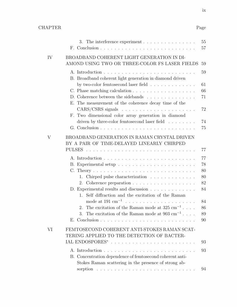
24 (a) Quantum beating between the two strong Raman lines in

PbWO4 measured by using a fs probe pulse with ν between

pump and Stokes pulses equal to 720 cm−1. (b) The cross section

from (a), which can be used to get the fitting parameters. The

beating has a frequency of 106.5 rad/ps, which corresponds to

the Raman shift difference of 565 cm−1 between the two modes.

(c)The coherence decay of the simultaneously excited strong Ra-

man lines measured when fs pump, Stokes pulses and a narrow-

band ps probe (about 1 nm spectral width) are applied to the

crystal. . . . . . . . . . . . . . . . . . . . . . . . . . . . . . . . . . . 54

25 UV probe pulse intensity as a function of probe delay and pump

delay. When three beams overlap in time, the UV gets absorbed.

(b) cross section of (a) at a zero delay of the pump pulse. The dip

width corresponds to the group velocity delay of the pump and

probe pulses. (c) CARS signal. . . . . . . . . . . . . . . . . . . . . . 55

26 Histograms of AS 5 pulse energy. Solid black bars: the number of

pulses (out of 150) vs. AS 5 pulse energy generated with Red and

IR input beams only. White bars: the histogram of AS 5 pulse

energy (913 pulses total) with the addition of the third input

beam. The dotted curve is a theoretical prediction obtained as-

suming perfect single-shot coherence of the two interfering fields,

and random shot-to-shot variation of their relative phase. . . . . . . 56

27 The broadband generation in diamond with the two input beams

(λ1= 630 nm and λ2= 584 nm, δν= 1250 cm−1) crossing at angles

of 3 and 5.8. Top: The generated beams are projected onto a

white screen. The two pump beams, S 1 and the first few AS

beams are attenuated (after the sample) by a neutral-density fil-

ter. The AS 2 spot clearly shows two different colors, with blue

corresponding to the Raman generation and green to the FWM

signal. Bottom: Normalized spectra of the generated sidebands. . . . 61

xvii

FIGURE Page

28 The sideband frequency as a function of the sideband order (a) and

as a function of the sideband output angle (b) with the two input

beams (λ1=630 nm and λ2=584 nm, δν= 1250 cm−1) crossing at

two different angles, 3 (square) and 5.8 (round). The sidebands

generated at 5.8 have a larger (about twice) frequency spacing

compared to the 3 case. . . . . . . . . . . . . . . . . . . . . . . . . 62

29 The Sideband frequency and output angle at the different detun-

ings (ν vary from 820 cm−1 to 2608 cm−1) between the pump

(fixed at 594 nm) and Stokes pulses. The output angles do not

vary much, nor does the the frequencies of the sidebands, although

ν varies a lot. . . . . . . . . . . . . . . . . . . . . . . . . . . . . . 63

30 The generation pictures and the pulse time responses in two dif-

ferent situations: (a) ν is tune close to resonance with the Ra-

man transition and (b) the Stokes and the pump wavelengths are

phase-matched at the chosen angle. When ν is on resonance

with the Raman transition, the Stokes get amplified. . . . . . . . . . 64

31 The intensity of the sideband AS 1, AS 2 and AS 10 as a function

of the polarization angle of the Stokes beam. The pump and the

Stokes beams have parallel polarization at 0 and 180 degrees. . . . . 66

32 Theoretical calculation of the frequency of AS 1 when the two

pump beams (λS=630 nm, λp=581.23 nm, δν=1332 cm−1, exactly

the Raman frequency) cross at an angle of 2.6, 3.6 and 4.6 degrees,

respectively. The phase matching angle between the two input

beams is 3.6 degrees. The sample thickness is 500 µm. . . . . . . . . 69

33 The sideband generation in diamond at the different delays be-

tween the two pump pulses (λ1= 630 nm and λ2= 584 nm, δν=

1250 cm−1). The time delay between each picture is about 20 fs.

We see at certain delays, the high-order sidebands are brighter

than the lower ones. . . . . . . . . . . . . . . . . . . . . . . . . . . . 70

34 “Green” sideband energy under different conditions. Black solid

line: all three input pulses are present. Red dotted line: IR and

Red pulses present only. Green dashed line: Yellow and Red

pulses present only. Top: the input beam geometry. . . . . . . . . . . 71

xviii

FIGURE Page

35 The CARS and CSRS signals observed in diamond using a UV

probe pulse. Top, the spectra of the CARS (left, center wave-

length is 305 nm) and CSRS (right, center wavelength is 332 nm)

as a function of the probe delay. Bottom, the exponential decay

time of the CARS (left) and CSRS (right) signals. . . . . . . . . . . 73

36 The 2-D array generation in diamond with three input pulses

(λpump= 720 nm, λStokes= 800 nm, and λprobe= 600 nm). The

wavelengths of the sidebands are labelled in nm. The degenerate

FWM signal (2Y-IR, a shorthand of 2ωY − ωIR) from the probe

and Stokes pulses and the one (2Y-R) from the probe and pump

pulses are much stronger than the Raman generation spots. They

either superimpose or shift slightly. The six-wave-mixing signal

(3Y-2R) from the pump and probe pulses is also visible. . . . . . . . 74

37 Schematic of the experimental setup. VF: Variable neutral den-

sity filter; BS: 50/50 ultrafast beam splitter. An approximately

linearly chirped pulse is obtained by misalignment of the compres-

sor in the amplifier. It is split into two and later recombined at

the sample with a relative time delay. . . . . . . . . . . . . . . . . . 78

38 Schematic of a compact compressor. Adapted from the laser train-

ing material, Coherent. . . . . . . . . . . . . . . . . . . . . . . . . . . 79

39 (a) The schematics of the pulses for the Raman excitation; (b)

The chirp of the pulses measured with SD-FROG; (c) Multiple

orders of the self diffraction signals in the crystal. . . . . . . . . . . . 82

40 Broadband generation in a PbWO4 crystal using two time-delayed

linearly chirped pulses applied at an angle of 1.2 to each other.

The chirp rate of the pulse is about 2100 cm−1/ps. (a) Generated

beams projected onto a white screen. (b) Normalized spectra of

the generated sidebands from AS 11 to AS 37. The wavelength

is in reciprocal scale. (c) The peak frequency of the generated

sideband plotted as a function of the sideband order. Multiple

value corresponds to the multiple peaks in the sideband spectrum.

The high-order sidebands have a slope of 200 cm−1 per AS order. . . 85

xix

FIGURE Page

41 (a) Broadband generation in PbWO4 crystal pumped by fs pulses

(λS=804 nm, λS=766 nm, and ν= 617 cm−1). The angle be-

tween the pump and Stokes beam is 2.9 . A third probe pulse (Y)

leads to generation of many orders of CARS and CSRS signals.

(b) Broadband generation in a PbWO4 crystal using two time-

delayed linearly chirped pulses applied at an angle of 2.4 to each

other. The chirp of the pulse is about 2100 cm−1/ps. (c) The

generated beams by using a pair of linearly chirped pulses with a

large chirp rate, 440 cm−1/ps. d) The intensity modulation of the

generated sidebands. . . . . . . . . . . . . . . . . . . . . . . . . . . . 87

42 Comparison of the sideband generation in PbWO4 crystal using

two near transform limited fs pulses (δν=615 cm−1) and a pair of

time-delayed chirped pulses. Many more sidebands are generated

in the latter case. . . . . . . . . . . . . . . . . . . . . . . . . . . . . . 88

43 Sideband generation in a PbWO4 crystal using two time-delayed

linearly chirped pulses applied at an angle of 4 to each other.

The chirp of the pulse is about 620 cm−1/ps. (a) Generated beams

projected onto a white screen. Pictures are taken at three consec-

utive time delays between the two pump beams, with a increase

of 33.3 fs. (b) The picture of the high-order sidebands. They are

brighter than the low-order sidebands. (c) Normalized spectra of

the two pump beam and the generated sidebands (left) and the

peak sideband frequency plotted as a function of the sideband

order (right). The slope is around 540 cm−1 per AS order. . . . . . . 89

44 Schematics of the experimental setup. OPA, optical parametric

amplifier; D1, D2, D3, delay stages; SM, spherical mirror; UG11,

UV bandpass filter; CCD: charge coupled device. Inset, CARS

and CSRS generation in a folded boxCARS geometry. . . . . . . . . 95

45 CARS pulse energy as a function of probe pulse delay at differ-

ent NaDPA concentrations. Sample, NaDPA solution in a quartz

cuvette with 2 mm path. The pH value of the solution is about 14. . 97

xx

FIGURE Page

46 Log-log plot of CARS pulse energy at the peak of the oscillation

as a function of NaDPA concentration. The solid curve is the the-

oretical curve obtained with the phase-matching factor included;

the dashed curve is the theoretical curve obtained with the as-

sumption ks = 0; at lower concentration, this curve has a slope

of 2. . . . . . . . . . . . . . . . . . . . . . . . . . . . . . . . . . . . . 98

47 Log-log plot of CSRS pulse energy at the peak of the oscillation as

a function of NaDPA concentration. Solid line is the theoretical

curve obtained with the phase matching factor included; dashed

line is the theoretical curve obtained with the assumption ks =

0; at lower concentration, this curve has a slope of 2, as is the case

for CARS signal. . . . . . . . . . . . . . . . . . . . . . . . . . . . . . 99

48 Refractive index of 50 mM and 100 mM NaDPA solution in the

UV range. Dashed line: fitting curve for 50 mM NaDPA solution;

dotted line: fitting curve for 100 mM NaDPA solution; solid line:

fitting curve from the empirical equation for water. . . . . . . . . . . 103

49 Logarithmic contour plot of the CARS signal spectrogram as a

function of the probe laser delay, acquired with CCD from a 50

mM sample of DPA in H2O/NaOH in a 100 µm quartz cuvette.

Exposure time is 10 s. . . . . . . . . . . . . . . . . . . . . . . . . . . 106

50 CARS signal concentration dependence for NaDPA solution in a

100 µm cell. The error is estimated from the three sets of data

taken at each concentration; c is a constant. . . . . . . . . . . . . . . 107

51 Two different forms (flake and needle) of crystalline DPA grown

under different conditions. . . . . . . . . . . . . . . . . . . . . . . . 108

52 CSRS signals in DPA crystal depends on whether the focal plane

of the laser beam is parallel to one of the long axis of the crystal

(left) or not (right). Top: Degenerate FWM in crystalline DPA. . . . 109

53 Schematics of the molecule in a crystal interacting with the light.

The orientation of its axis with respect to the laser polarization

will determine which molecular mode interacts with light, and

how strongly. . . . . . . . . . . . . . . . . . . . . . . . . . . . . . . 110

xxi

FIGURE Page

54 CSRS signal in DPA crystal (needle form) at different orientations

of the needle. . . . . . . . . . . . . . . . . . . . . . . . . . . . . . . . 111

55 (a) Nuclear fusion in a hot plasma “soup”; and (b) nuclei pre-

aligned for a laser-induced collision. . . . . . . . . . . . . . . . . . . . 114

56 Classical simulation of a laser-induced nuclear collision between

H+ and T+. Part (a) shows the single-cycle laser pulse; part (b)

shows the calculated nuclear motion; part (c) shows the distance

between the nuclei at the time the collision happens; part (d)

shows the second derivative of the system’s dipole moment p,

which results in an X-ray burst of sub-attosecond (10−18s) duration. . 117

57 Classical simulation of a nuclear collision between H+ and T+

induced by an elliptically polarized laser pulse. (a) the electrical

field of the ultrashort pulse; (b) the motion of the two nuclei in x

direction; (c) the motion of the two nuclei in y direction; (d) the

distance between the two nuclei when the collision happens; (e)

the short pulse generated due to the collision; (f) two-dimensional

trajectories of the two nuclei. . . . . . . . . . . . . . . . . . . . . . . 119

58 The motion of the two nuclear ensembles under the action of ellip-

tically polarized laser field. Clouds of red dots show the ensemble

of T+ nuclei at different moments of time projected onto the X-Y

plane; blue dots show the D+ ensemble. Dashed lines are the clas-

sically calculated parametric trajectories for a single pair of nuclei

(D+ and T+) under the same laser field as used in the ensemble

calculation, but with initial positions and velocities precisely right

for a collision. . . . . . . . . . . . . . . . . . . . . . . . . . . . . . . . 120

59 Simulation of a laser-induced nuclear collision between H+ and

T+. (a) collision picture in the lab frame (H+, dotted curve, T+,

solid curve), insert: the sub attosecond (2.4×10−20 s) pulse gen-

erated at the collision point; (b) calculated nuclear motion in the

center of mass frame(classical, solid line, quantum, scattered di-

amond), insert: initial Gaussian wavepacket used for the numer-

ical solution of the Schrodinger equation. (c) movement of the

wavepackets around the collision point; (d) probability density

plots of the wavepackets at different time. . . . . . . . . . . . . . . . 126

xxii

FIGURE Page

60 (a) (Solid line) Minimum internuclear distance as a function of the

peak electric field from a 1-d quantum-mechanical calculation; (b)

(dotted line) Minimum internuclear distance calculated from 1.4

Up; (c) (dash-dotted line) Closest approach (collision) time vs.

the peak electric field. . . . . . . . . . . . . . . . . . . . . . . . . . . 129

61 Classical simulation of a nuclear collision between H+ and T+

induced by an elliptically polarized laser pulse. (a) the motion of

the two nuclei in the lab frame(H+, solid curve, H+, dotted curve);

(b) the motion of the two nuclei in the center of mass frame. . . . . 132

62 Contour plots of the probability density of the wavepackets at

different times: (a) t=0; (b) t=306; (c) t=413.5; (d) t=418. The

contour lines are on logarithmic scale. . . . . . . . . . . . . . . . . . 133

63 Absorption cross section of NaDPA solution in UV range. . . . . . . 151

1

CHAPTER I

INTRODUCTION

The generation of ultrashort pulses is made possible by the technique of modelocking,

which was first demonstrated in 1964 when nanosecond (ns) mode-locked pulses were

produced [1]. First femtosecond (fs) laser pulses were generated using dye lasers in

1975 [2]. Later solid-state material was developed, which made the reliable and tun-

able pulsed laser available. The most attractive material is titanium-doped sapphire

crystals (Ti:Sapphire, Al2O3:Ti3+), which has extremely wide gain bandwidth (from

660 nm to 1180 nm) and makes the generation of 4 fs possible if this bandwidth is

modelocked. With the important modelocking technique—“Kerr-lens modelocking”

observed in 1991 [3], 6.5 fs pulses from a Ti:Sapphire laser were generated in 1997 [4].

This was by then the shortest pulse ever generated directly from a laser. Nowadays,

commercial laser systems routinely produce sub-100 fs pulses and these pulses are

finding applications in many fields. In 1999 Nobel Prize in Chemistry was awarded to

Professor Ahmed H. Zewail “for showing that it is possible with rapid laser technique

to see how atoms in a molecule move during a chemical reaction” using fs pulses.

Short pulse generation requires a wide phase-locked spectrum. Earlier the short

pulses were obtained by expanding the spectrum of a mode locked laser by self phase

modulation (SPM) in an optical fiber and then compensating for group velocity dis-

persion (GVD) by diffraction grating and prism pairs. Pulses as short as 4.4 fs have

been generated [5]. For ultrafast measurements on the time scale of electronic motion,

generation of subfemtosecond pulses is needed. Generation of subfemtosecond pulses

with a spectrum centered around the visible region is even more desirable, due to the

This dissertation follows the style of Physical Review A.

2

fact that the pulse duration will be shorter than the optical period and will allow sub-

cycle field shaping. As a result, a direct and precise control of electron trajectories

in photoionization and high-order harmonic generation will become possible. But to

break the few-fs barrier new approaches are needed.

In recent past, broadband collinear Raman generation in molecular gases has

been used to produce mutually coherent equidistant frequency sidebands spanning

several octaves of optical bandwidths [6]. It has been argued that these sidebands

can be used to synthesize optical pulses as short as a fraction of a fs [7]. The Ra-

man technique relied on adiabatic preparation of near-maximal molecular coherence

by driving the molecular transition slightly off resonance so that a single molecular

superposition state is excited. Molecular motion, in turn, modulates the driving laser

frequencies and a very broad spectrum is generated, hence the term for this process

“molecular modulation”. By phase locking, a pulse train with a time interval of the

inverse of the Raman shift frequency is generated. While at present isolated attosec-

ond X-ray pulses are obtained by high harmonic generation (HHG) [8], the pulses are

difficult to control because of intrinsic problems of x-ray optics. Besides, the con-

version efficiency into these pulses is very low (typically 10−5). On the other hand,

the Raman technique shows promise for highly efficient production of such ultra-

short pulses in the near-visible spectral region, where such pulses inevitably express

single-cycle nature and may allow non-sinusoidal field synthesis [7].

In the Raman technique ns pulses are applied for preparing maximal coherence

when gas is used as a Raman medium. When the pulse duration is shorter than the

population relaxation time T2 (T2 = 1πc∆νR

, ∆νR is the spontaneous Raman linewidth),

the response of the medium is a highly transient process, i.e. the Raman polarization

of the medium doesn’t reach a steady state within the duration of the pump pulse. In

this transient stimulating Raman scattering (SRS) regime, a large coherent a mole-

3

cular response is excited. It has been shown that the SRS gain increment explicitly

depended on the integral cross section and was independent of the peak cross section

of spontaneous Raman scattering as the ratio between the pumping pulse width (11

picosecond (ps)) and the time of optical dephasing of molecular vibrations changed

from 0.42 to 9.3 in the spontaneous Raman scattering study of several oxide cyrstals

[9]. The advantage of using a short pulse is that the number of the pulse in the train

will be reduced compared with the ns Raman technique. But when a single fs pump

is used, the strong self phase modulation (SPM) suppresses the Raman generation

[10]. When a pulse duration is reduced to less than a single period of molecular vibra-

tion or rotation, an impulsive SRS regime is reached [11]. In this regime, an intense

fs pulse with a duration shorter than the molecular vibrational period prepares the

vibrationally excited state and a second, relatively weak, delayed pulse propagates in

the excited medium in the linear regime and experiences scattering due to the modu-

lation of its refractive index by molecular vibrations, which results in the generation

of the Stokes and anti-Stokes sidebands [12]. This technique has the advantage of

eliminating the parasitic nonlinear process since it is confined only within the pump

pulse duration.

A closely related approach which is called four-wave Raman mixing (FWRM)

for generating ultrashort pulses using two-color stimulated Raman effect is proposed

in 1993 by Imasaka [13]. It is based on an experimental result his student has stum-

bled on. Shuichi Kawasaki was trying to develop a tunable source for thermal lens

spectroscopy and he noticed bright, multicolored spots out of the Raman cell pressur-

ized with hydrogen, which they called “Rainbow Star” [14]. The applied beam was

supposed to be monochromatic but it actually had two color in it. To confirm the

FWRM hypothesis, a nonlinear optical phenomenon in which three photons interact

to produce a fourth photon, they used two-color laser beams with frequencies sepa-

4

rated by one of the rotational level splittings for hydrogen (590 cm−1). Indeed, they

observed the generation of more than 40 colors through the FWRM process, which

provided a coherent beam consisting of equidistant frequencies covering more than

thousandths cm−1 in frequency domain [15]. This FWRM process resulted in the

generation of higher-order rotational sidebands at reduced pump intensity compared

to the stimulated Raman scattering. The generation of the FWRM fields required

phase matching and were coherently phased, and therefore had the potential to be

used to generate sub-fs pulses [16].

Later ps pulses [17], ps and fs pump pulses [18], and a single fs pulse [10] were

used to find the optimal experimental conditions for efficient generation of high-order

rotational lines. Generally speaking, when the additional Stokes field is supplied

rather than grown from quantum noise, advantages include: high-order anti-Stokes

generation, higher conversion efficiency, and improved reproducibility of the pulses

generated, as shown in earlier experiments with gas in ns regime [19]. Recently,

efficient generation of high-order anti-Stokes Raman sidebands in a highly transient

regime is also observed using a pair of 100-fs laser pulses tuned to Raman resonance

with vibrational transitions in methane or hydrogen [20; 21]. They found that in

this transient regime, the two-color set-up permits much higher conversion efficiency,

broader generated bandwidth, and suppression of the competing SPM. The high

conversion efficiency observed proves the preparation of substantial coherence in the

system although the prepared coherence in the medium cannot be near maximal as

in the case of the adiabatic Raman technique.

Almost all these works are carried out using a simple-molecule gas medium such

as H2, D2, SF6 or methane since the gas has negligible dispersion and long coher-

ence lifetime. Molecular gas also has a few other advantages as a Raman medium.

They are easily obtainable with a high degree of optical homogeneity and have high

5

frequency vibrational modes with small spectral broadening, which leads to large Ra-

man frequency shifts and large Raman scattering cross sections. However, a Raman

gas cell with long interaction length is needed due to the lower particle concentration

[22].

How about solids Raman medium such as Raman crystal? As we know, the

high density of solids results in the high Raman gain. The higher peak Raman cross

sections in crystals result in lower SRS thresholds, higher Raman gain, and greater

Raman conversion efficiency [22]. In addition, there is no need for cumbersome vac-

uum systems when working with room temperature crystals, and therefore a compact

system can be designed.

The difficulty in using crystals is the phase matching between the sidebands be-

cause the dispersion in solids is significant. Sideband generation using strongly driven

Raman coherence in solid hydrogen is reported but the generation process is very close

to that of H2 gas and solid hydrogen is a very exotic material [23]. Observation of

generation with few sidebands (Stokes or Anti-Stokes) in other solid material is noth-

ing new. About two decades ago, Dyson et. al. has observed one Stokes and 1 AS

generated on quartz during an experiment designed for another purpose [24]. Later,

there were numerous works of using Raman crystals for building Raman lasers which

extended the spectral coverage of solid-state lasers by using SRS [25]. A detailed

review of crystalline and fiber Raman lasers is given by Basiev [26]. The Raman

spectroscopy of many crystals for SRS is therefore available because of this particular

usage for building Raman lasers [27]. The Raman lasers are normally pumped by

ns or ps pulses, which are comparable with the period of Raman-active vibration.

In particular, potassium gadolinium tungstate (KGd(WO4)2; KGW) crystal, a very

popular Raman crystal due to its high efficiency, has been studied with two-color fs

pulses using collinear configuration [28]. Only 2 S were observed. Later impulsive

6

Raman scattering was observed in KGW using 70 fs pulses and 2 AS and 1 S were

generated [29]. To our knowledge, no efficient generation using crystals had been

reported before our experiment.

Therefore this research is directed toward the development of efficient broadband

generation using Raman crystals. Since coherence lifetime in a solid is typically

shorter than in a gas, the use of fs (or possibly ps) pulses is inevitable when working

with room-temperature crystals. We choose PbWO4 (lead tungstate), which exhibits

good optical transparency, high damage threshold, and is non-hygroscopic. It is also

a popular crystal used for building Raman lasers using ns or ps pulsed pumping

[30]. Diamond is also used in our experiments since it has a narrow Raman line

at relatively large Raman frequency—1332 cm−1 with linewidth of 3.3 cm−1(T2=3.2

ps) [31]. Moreover, diamond has the highest atom density of any material and it

is transparent from far infrared to ultraviolet (above 230 nm) and has the widest

electromagnetic bandpass of any material which is very attractive for broadband

generation. We find that the main difference when working with crystal using two-

color laser fields excitation is the necessity of using non-collinear geometry of the two

applied fields so that the phase matching condition can be fulfilled. Phase matching

plays a crucial role as we will show later. We have successfully generated as many as

40 colors when using two-color fs pulses and as many as 50 colors when three-color fs

pulses are focused in the crystal. The effects of the polarization, the angle between

the two pump beams, and the detuning between the two pump laser frequencies on

the sidebands generation are studied as well.

During our work, we noticed that similar experiments were carried out with

different crystals very recently. For example, high-order coherent anti-Stokes Raman

scattering (CARS) has been observed in YFeO3 and KTaO3 crystals when two-color

fs pulses were used [32; 33]. A multiple CARS generation in KNbO3 [33] and in TiO2

7

[34] have just been reported. We can see there is a growing interest in broadband

generation using Raman-active crystals.

The major part of this dissertation, including chapter II to V, is on the subject

of broadband sidebands generation in Raman crystals. In chapter II I give an in-

troduction to the basic concepts which are needed for the description of our work,

and a theoretical background for this Raman generation technique. In chapter III,

I present our experimental results on broadband light generation in PbWO4 using

fs pulses. In chapter IV, broadband light generation in diamond is given. A. M.

Zheltikov proposed the idea of using a sequence of short light pulses. When the time

interval between the pulses in the train is equal to the period of Raman vibrations,

the corresponding Raman-active mode is selectively excited [35]. This idea may be

especially suitable for solids since the competing nonlinear processes such as SPM can

be avoid using a pulse train while the coherence can still build up. We have extended

this idea to the efficient generation in PbWO4 using two time-delayed linearly chirped

pulses. This experiment is discussed in chapter V.

Spontaneous, stimulated, and coherent Raman scattering provide the basis for

Raman spectroscopy [36] which is a powerful tool widely used in chemistry, biology,

and engineering [36; 37; 38]. In early research, ns CARS spectroscopy has been used

for measuring the concentration of molecular species in combustion diagnostics [39].

In the time-resolved CARS technique [40], two pulses (pump and Stokes) are used to

create coherence at one or more Raman transitions. Then a third time-delayed probe

pulse is applied, which scatters from the coherence and generates the CARS and

coherent Stokes Raman scattering (CSRS) signals. By delaying the third pulse, the

strong instantaneous nonresonant background from FWM can be eliminated, which

renders femtosecond CARS superior to nanosecond CARS for the determination of

spectroscopic constants, especially under extreme conditions such as those in com-

8

bustion cells or flames [41]. Recently time-resolved femtosecond CARS spectroscopy

has been applied for measuring the gas-phase temperatures and concentrations [42].

Dipicolinic acid (DPA) is a marker molecule for bacterial spores [43] and the

ability to detect trace amounts is of paramount importance. We work with DPA

in a H2O/NaOH solution (NaDPA). Optical coherence of NaDPA has a relaxation

time of the order of 30 fs, and vibrational coherence in liquids has picoseconds time

scale. Femtosecond pulses therefore are essential for the study of a complex organic

molecule such as NaDPA. In chapter VI, we study concentration dependence of fs

CARS in the presence of strong absorption using a NaDPA solution. We also study

the CSRS in the crystalline DPA.

A variety of nonlinear processes becomes accessible thanks to the large inten-

sities of fs pulses. In chapter VII, I present a theoretical study of laser-controlled

nuclear fusion using superintense ultrashort (a few cycle) pulses. This dissertation is

summarized in chapter VIII.

9

CHAPTER II

BASIC CONCEPTS AND THEORY

In this chapter, I give some basic concepts for ultrashort pulses: the linear and non-

linear pulse propagation of a short pulse in a dispersive medium and the resultant

nonlinear effects such as self phase modulation and self focusing, which are encoun-

tered frequently in our experiment using fs pulses. An introduction to the Raman

scattering, which is crucial to this work, is given here. The terms including four wave

mixing, coherent anti-Stokes Raman scattering, coherent Stokes Raman scattering,

and four wave Raman mixing, which are often used in the related references and this

work, are given here too. After that I briefly mention an ultrafast pulse measure-

ment technique—self diffraction frequency-resolved optical gating, which is used in

our experiment to characterize the chirp of a pulse.

In the theory part I give a derivation for the Hamiltonian of the molecular system

including the interaction with the laser field. In order to show how the propagation

of the two fields leads to the sidebands generation, we perform an approximate theo-

retical calculation using the crystal PbWO4 as an example.

A. Basic concepts

1. Linear pulse propagation in a dispersive medium

When a pulse propagates in a dispersive medium, the pulse gets broadened because

frequency components within the pulse travel with different phase velocity Vφ = cn(λ)

,

where c is the speed of light and n(λ) is the refractive index at this wavelength. This

leads to a chirped pulse, where the instantaneous frequency varies over the temporal

pulse. A pulse is called linearly chirped when the phase has a quadratic variation, i.e.

10

the frequency varies linearly with time delay. The frequency of a positively chirped

pulse increases as a function of time delay, while the frequency of a negatively chirped

pulse decreases vs. time. The pulse length increases due to the chirp and consequently

the peak intensity of the pulse decreases. We can use it to our advantage as will be

shown in chapter V. Here I give a derivation of a pulse output width from a dispersive

medium as a function of the input pulse length and the group delay dispersion.

a. Pulse broadening

The electric field of a gaussian pulse with width (FWHM) τin, amplitude E0, and

center frequency ω0 can be written as:

Ein(t) = E0 exp(−2 ln 2t2

τ 2in

− iω0t). (2.1)

The fourier transform of the electric field is:

Ein(w) =1√2π

∫ ∞

−∞Ein(t) exp(iωt)dt = α exp[−τ

2in(ω − ω0)

2

8 ln 2]. (2.2)

Here α = E0τin2√

ln 2is a constant. The electric field of the output pulse is [44]:

Eout(w) = Ein(w) exp−i[φ+ (ω − ω0)φ′ +

φ′′

2(ω − ω0)

2] (2.3)

= α exp(−iφ) exp(−i(ω − ω0)φ′) exp[−(

τ 2in

8 ln 2+iφ′′

2(ω − ω0)

2].

Here φ′ is the group delay and φ′′ is the group delay dispersion (GDD). The high-

order terms such as third-order dispersion (TOD) are neglected. Let ω′

= ω = ω0

11

and Γ = −(τ2in

8 ln 2+ iφ′′

2), then

Eout(t) =

∫ ∞

−∞Eout(ω) exp(−iωt)dω (2.4)

= α

√π

Γexp[−i(φ− ω0t)] exp[−(φ′ − t)2

4Γ]

= α′exp

[−i(φ− ω0t) − (φ′ − t)2

τ2in

2 ln 2+ 2iφ′′

].

Let’s redefine Γ = (τ2in

2 ln 2+ 2iφ′′)−1, then the output field has the form of

Eout(t) = E0 exp[i(ω0t− φ) − Γ(t− φ′)2] (2.5)

= E0ei(ω0t−φ)e

2iφ′′

τ4in

4(ln 2)2+4φ′′2(t−φ′)2

e

−

τ2in

2 ln 2τ4in

4(ln 2)2+4φ′′2(t−φ′)2

.

We finally get the expression for the output pulse width versus the input pulse width

as:

τoutτin

=

√1 +

φ′′2

τ 4in

∗ 16(ln 2)2 (2.6)

The phase change for a pulse through a dispersive medium l is φ = kz = 2πλ

(ln) =

ωcln. Here n is function of frequency and wavevector k=2π/λ. We can write

φ(ω) =ωln(w)

c. (2.7)

The GDD φ′′ as a function of λ and d2ndλ2 can be calculated as follows.

φ′′ =d2φ

dω2=l

c(ωd2n

dω2+ 2

dn

dω). (2.8)

Since

dn

dω=dn

dλ

dλ

dω= − λ2

2πc

dn

dλ; (2.9)

and

d2n

dω2=

d

dλ(dn

dω)dλ

dω=

λ4

4π2c2d2n

dλ2+

λ3

2π2c2dn

dλ. (2.10)

12

Therefore we have

φ′′ =d2φ

dω2=

λ3l

2πc2d2n

dλ2. (2.11)

Please note that the GDD always refers to some optical element (e.g. the GDD

of a 1-mm thick silica plate is 35 fs2 at 800 nm) or to some given length of a medium

(e.g. an optical fiber). If one specifies the GDD per unit length (in units of s2/m),

this is the group velocity dispersion (GVD) [45].

b. Effective interaction length

Due to dispersion of the material, different waves propagate at different group veloc-

ities. For femtosecond pulses, the interacting pulses may get separated after propa-

gating some distance in the medium, which means that there is a reduced effective

interaction length Leff . Thus Leff is an important parameter for choosing the thick-

ness of the crystal. Next I show how to calculate Leff .

Group velocity VG is defined as:

VG = (dk

dω)−1 =

c

n− λdndλ

. (2.12)

The group velocity mismatch (GVM) is defined as:

VG =

(1

VG,i− 1

VG,j

)−1

. (2.13)

where VG,i and VG,j are the group velocities of the two interacting waves i and j. The

interaction length Leff can be calculated by:

Leff = 2τp|VG| = 2τp

∣∣∣∣∣(

1

VG,i− 1

VG,j

)−1∣∣∣∣∣ . (2.14)

where τp is the input pulse duration at FWHM. For the crystal we use, the interaction

length of PbWO4 and diamond is about 0.5 mm and 1.2 mm respectively when pulses

13

with wavelength 580 and 640 nm are used. The interaction length is longer when a

pair of IR pulses are used due to the relatively smaller dispersion over this region.

2. Nonlinear pulse propagation

a. Self focusing and white light generation

Nonlinear optical phenomena arise when an intense short pulse interacts with a nonlin-

ear medium. In nonlinear optics, the optical response can be described by expressing

the polarization P (t) as a power series in the field strength E(t) as in [46]:

P (t) = χ(1)E(t) + χ(2)E2(t) + χ(3)E3(t) + · · · (2.15)

= P (1)(t) + P (2)(t) + P (3)(t) + · · ·

The constant of proportionality χ(1) is the linear susceptibility. The linear polariza-

tion of the material P (1)(t) gives rise to the linear optical effects such as refractive

index, dispersion and birefringence. The quantities χ(2) and χ(3) are the second-

and third-order nonlinear optical susceptibilities, respectively. The second order non-

linear polarization P (2)(t) is responsible for second harmonic generation, sum- and

difference-frequency mixing, and parametric generation.

The third order nonlinear polarization P (3)(t) is essential to this work and will be

described in detail here. First it is responsible for optical Kerr effect. A sufficiently

high laser field can induce a nonlinear refractive index response in the materials such

that the index n becomes intensity dependent as:

n = n0 + n2I (2.16)

where n0 is the usual linear or low intensity refractive index, n2 = 12π2

n20cχ(3) is an

optical constant that characterizes the strength of the optical nonlinearity, and I

14

is the intensity of the incident laser field. When a beam of light having a uniform

transverse intensity distribution propagates through a material in which n2 is positive,

the material acts as a positive lens, which causes the rays to curve toward each other.

The intensity at the focal spot of the self-focused beam is usually sufficiently large to

lead to optical damage of the material. We have observed this in the crystal sample

we use. The beam profile is drastically changed as shown in Fig. 1 (b).

Fig. 1. Nonlinear effects in crystal. (a) The intensity of the pump beams used are

below the threshold of self focusing. The sidebands generated are nice, round

spots. (b) The intensity of the pump beams used are above the threshold of

self focusing, which results in the deterioration of the generated beams. (c)

SPM causes pulse broadening as the pulse propagates through the crystal.

15

b. Self phase modulation and cross phase modulation

The intensity of an ultrashort pulse changes with time, hence different parts of the

pulse experience different magnitudes of refractive index. The time varying refractive

index produces a time-dependent phase modulation of the pulse and therefore con-

tributes to spectral broadening of the pulse, which is called self phase modulation

(SPM). Considering a pulse with center frequency ω0 propagating in a medium of

length L, the phase

φ(t) = ω0t− kz = ω0t− 2πn

λL. (2.17)

The instantaneous frequency is the derivative of the phase with respect to time as

given by:

dφ(t)

dt= ω0 − 2πL

λ

dn

dt= ω0 − 2πn2L

λ

dI(t)

dt. (2.18)

We see that the nonlinear refractive index induces an approximately linear chirp on

the pulse. If one pulse modifies the effective refractive index causing a second pulse

to change its characteristics, this is referred to as cross-phase modulation (CPM).

In our experiment, SPM causes the spectral broadening after the crystal as shown

in Fig. 1 (c) and CPM makes two pulses affect each other slightly. CPM provides

a very convenient way to find the zero delay of two interacting pulses. When the

intensity of a pulse is high enough, the pulse after a nonlinear medium is drastically

broadened in spectrum. The spectrally broadened pulse is referred to as a white-

light continuum pulse. White light generation is a very complicated process. Beside

SPM, and self-focusing, there are other nonlinear processes contributing to the white

light generation [47]. White light generation in glass can be used to find the focus

of the pulses as well as the time overlap between pulses since one can use a high

intensity beam without the concern of burning the glass.

16

3. Raman scattering

a. Linear Raman scattering

I’d like to pay some tribute to the great scientist Raman here. It is in March 1928 that

professor Raman announced his discovery of Raman scattering, which he called a new

secondary radiation. “The apparatus used by Raman for the discovery consisted of a

mirror for deflecting sunlight, a condensing lens, a pair of complementary glass filters,

a flask containing benzene and a pocket spectroscope. the total cost not exceeding $25”,

as described by R. S. Krishnan [48]. Raman observed not only the Stokes radiation,

which has the lower photon energy than the incident photon, but the extremely weak

anti-Stokes radiation.

Raman scattering is an inelastic collision of an incident photon with a mole-

cule. Following the collision, a photon with either frequency ωS = ωl − ωR or

ωAS = ωl−ωR is scattered. Here ωR is the vibrational frequency of the molecule. The

former one is called Stokes radiation. In the latter case, the photo ωl is scattered by

an excited molecule and is called anti-Stokes radiation. This process is illustrated

in Fig. 2. The intermediate state of the system during the scattering process is often

called “virtual state” (dotted line in Fig. 2 (a) and (b)). Since in thermal equilib-

rium the population of level n is smaller than the population in ground state g by

the Boltzmann factor exp(−ωng/kT ), most molecules will initially be in the ground

state. Consequently, the anti-Stokes radiation is much weaker than the Stokes radia-

tion. If the virtual level coincides with one of the molecular eigenstates, one speaks

of the resonance Raman effect. As a result of the resonance, the Stokes or anti-

Stokes radiation can be dramatically enhanced. Both Boyd [46] and Demtroder [49]

give an excellent description of the Raman scattering. Here I just briefly write some

of the formulas which are important for understanding the work presented in this

17

dissertation.

The dipole moment of a molecule under an electric field E = E0 cos(ωt) can be

written as:

p = µ0 + αE. (2.19)

The first term µ0 represents a possible permanent dipole moment while αE is the

induced dipole moment. α is called the polarizability. The dipole moment and po-

larizability can be expanded into Taylor series in the normal coordinates qn of the

nuclear displacements as:

µ = µ0 +

Q∑n=1

(∂µ

∂qn

)0

qn + . . . , (2.20)

αij(q) = αij(0) +

Q∑n=1

(∂αij∂qn

)0

qn + . . . . (2.21)

For small vibrational amplitudes the normal coordinates qn(t) of the vibrating

molecule can be approximated by

qn(t) = qn0 cos(ωRt), (2.22)

ωR is the vibrational frequency. Inserting Eq. 2.20 and Eq. 2.21 to into Eq. 2.22

yields the total dipole moment [49]

p = µ0 +

Q∑n=1

(∂µ

∂qn

)0

qn0 cos(ωnt) + αij(0)E0 cos(ωt) (2.23)

+1

2E0

Q∑n=1

(∂αij∂qn

)0

qn0[cos(ω + ωR)t+ cos(ω − ωR)t].

The last term describes the Raman scattering. We can see that two inelastically

scattered components with the frequencies ω − ωR (Stokes waves) and ω + ωR (anti-

Stokes waves) are produced. The mode with polarizability change ∂α∂q

= 0 is called a

18

Raman-active mode.

b. Stimulated Raman scattering

This spontaneous Raman scattering process has very low efficiency. Typically only

approximately 1 part in 106 of the incident radiation will be scattered into the Stokes

frequency. When the laser beam intensity becomes sufficiently large, highly efficient

scattering can occur as a result of the process called stimulated Raman scattering

(SRS). It is described in detail in Boyd’s book [46]. Here I just give some of the

relevant equations.

The expression for the Stokes polarization is:

PNLS (z, t) = P (ωS) exp(−iωSt) + c.c. (2.24)

The complex amplitude P (ωS) is given by:

P (ωs) = 6χR(ωS)|AL|2AS exp(ikSz). (2.25)

Assume the total optical field can be represented as:

E(z, t) = AL exp[i(kLz − ωLt)] + AS exp[i(kSz − ωSt)] + c.c.. (2.26)

Here χR(ωS) is a shortened form of χ3(ωS = ωS + ωL − ωL) and is given by:

χR(ωS) =(N/6m)

(∂α∂q

)2

0

ω2R − (ωL − ωS)2 + 2i(ωL − ωS)γ

. (2.27)

Here γ is the damping constant, N is the density of the molecules and m is the reduced

nuclear mass.

The evolution of the Stokes field AS is given in the slowly-varying amplitude

19

approximation by

dASdz

= −αSAS (2.28)

where

αS = −12πiωs

nscχR(ωS)|AL|2 (2.29)

is the Stokes wave “absorption” coefficient which has a negative real part, implying

that the Stokes wave has exponential growth. Raman Stokes amplification is a process

for which the phase-matching condition is automatically satisfied. For anti-Stokes

waves, there is a similar expression as Stokes waves. And there is another contribution

that depends on the Stokes amplitude. The total polarization at the AS frequency is

given by:

P (ωa) = 6χR(ωa)|AL|2Aa exp(ikaz) + 3χF (ωa)A2LA

S exp[i(2kL − kS)z] (2.30)

Here χF (ωa) = χ3(ωa = 2ωL−ωS) is a FWM susceptibility. Similarly there is a FWM

contribution to the Stokes polarization. Assuming optically isotropic medium, slowly

varying amplitude and constant pump approximations, the field amplitude of AS and

S field obey the coupled equations:

dASdz

= −αSAS + κSA∗aeikz, (2.31)

dAadz

= −αaAa + κaA∗Se

ikz. (2.32)

When the wavevector mismatch k = (2kL − kS − ka) is small, the FWM term

is an effective driving term. Perfect phase matching can always be achieved if the

Stokes wave propagates at some nonzero angle with respect to the laser wave.

For SRS, the Stokes field and anti-Stokes field generated can have higher ef-

ficiency, specially when an external cavity is used. Many Raman lasers, based on

the SRS process, have been built using nonlinear crystals [25]. The phenomenon

20

of high-order stimulated Raman lines simultaneously generated over a wide spectral

region is called four-wave Raman mixing (FWRM) [10]. For example, FWRM

in crystal PbWO4 has been observed up to 9th order [30]. We have mentioned four

FWMsignal

FWM= 3+ 1 2

P

n= P+(n-1) R

S

R

L

StokesSignal, S

Anti-StokesSignal, AS

L

R

CARS= L+ R

CARSSignal, AS

L

S

R

CSRS= L- R

CSRSSignal, S

L

S

R

FWRM

(a) (b)

(c) (d)

(e) (f)

Fig. 2. Schematic level diagrams for different processes. (a) anti-Stokes Raman scatter-

ing; (b) Stokes Raman scattering; (c) CARS (d) CSRS; (e) FWM; (f) FWRM.

wave mixing susceptibility in the above description. Four wave mixing (FWM)

is a general term for a process in which a frequency is created from the three other

21

frequencies ω4 = (±ω1) + (±ω2) + (±ω3). Third harmonic generation is a special

case of FWM in which ω1 = ω2 = ω3, and ω4 = 3ω1. In coherent anti-Stokes

Raman scattering (CARS), a special case of FWM, the two laser field are chosen

such that ω1 − ω2 = ωR. These two waves generate a large population density of vi-

brationally excited molecules. These excited molecules act as a nonlinear medium for

the generation of AS radiation at ωCARS = 2ω2−ω1. CARS is also called a four-wave

parametric mixing process. The intensity I of the CARS signal is [49]

I ∝ |χ(3)|2N2I1(ω1)2I2(ω2) (2.33)

Here N is the molecular density and I1(ω1) and I2(ω2) are the pump laser intensi-

ties. Another similar process is coherent Stokes Raman scattering (CSRS) in

which a frequency ωCSRS = 2ω1 − ω2 is generated. The different processes are shown

schematically in Fig. 2.

4. Ultrashort pulse measurement method—SD FROG

To measure an event in time, you must use a shorter one. How to measure a shortest

pulse ever created is a difficult problem which is addressed by a book ”Frequency-

Resolved Optical Gating: The Measurement of Ultrashort Laser Pulses” [50]. Here

I will just briefly mention one method which is easy to set up and is used in our

experiment—SD Frequency-Resolved Optical Gating (FROG).

Self diffraction (SD) is also a χ(3) nonlinear process in which the three interac-

tive pulses are replica of each other. It is also called forward four-wave mixing. Here

I give a brief description of this powerful pulse measuring method. The schematics

of the SD FROG is shown in Fig. 3 [51]. The signal pulse field has the form of:

Esig(t, τ) = E(t)2E∗(t− τ) (2.34)

22

Fig. 3. Schematics of the SD FROG. The signal pulse is centered at approximately the

time τ/3 of one input pulse (From D. J. Kane and R. Trebino, IEEE Journal

of Quantum Electronics, Vol. 29, 571 (1993)).

and the measured signal intensity is

IFROG(ω, τ) = |∫ ∞

−∞E(t)2E∗(t− τ) exp(−iωt)dt|2. (2.35)

Assuming it is a gaussian pulse E(t) = exp(− t2

τ2 ), then

Esig(t, t0) = exp(−t2

t20) exp[−(t− τ)2

t20] exp[−(t− τ)2

t20] (2.36)

= exp[−t2

t20− 2

(t− τ)2

t20]

From ddt

(Esig(t, t0)) = 0, one can find that the signal pulse has a maximum at approx-

imately the time τ/3 of one input pulse as shown in Fig. 3 inset. The instantaneous

frequency of the signal pulse is

Ωsig(τ) = 2ω(τ/3) − ω(−2τ/3). (2.37)

As a result, for the case of linear chirp, if the FROG signal frequency is Ωsig(τ) = βτ ,

then ω(τ) = 3/4βτ . This formula will be used in chapter VIII when the subject of

23

chirped pulse excitation is discussed.

B. Hamiltonian derivation and sidebands generation

As described in the introduction, our method of generating broadband sidebands in

crystals uses two pump fields, which are tuned close to the Raman frequency. These

two fields prepare the molecular coherence. The coherent molecular motion modulates

light and produces the sidebands. In this section I derive the Hamiltonian using an

approach following Hickman’s description [52] which arrives at the same formulas as

shown in [53]. All the equations are in terms of z and the retarded time t = tlab−z/c.The field propagation which produces the sidebands is shown in [53].

First we write the time-dependent wave function in terms of an expansion of zero

field eigenfunctions:

H0|n >= Wn|n > (2.38)

ψ =∑n

Cne−iWnt|n > (2.39)

The time dependent Schrodinger equation has the form of:

(H0 + V )|n >= i∂ψ

∂t(2.40)

Using Eq. 2.38 and Eq. 2.39 we have:

∑n

Cne−iWnt(H0 + V )|n >= i

∑n

(∂Cn∂t

− iWnCn)e−iWnt|n > (2.41)

Rearranging the terms we get:

∑n

i(dCndt

− CnV )e−iWnt|n >= 0 (2.42)

24

Applying < j| to the above equation, we have:

∑n

< j|i(dCndt

− CnV )e−iWnt|n >= 0; (2.43)

idCndt

e−iWjt =∑n

< j|CnV |n > e−iWnt. (2.44)

Exchanging index j with n and letting Wjn = Wj −Wn, we obtain:

idCndt

=∑j

< n|V (t)|j > Cje−iWjnt. (2.45)

The interaction potential can be written as:

V = −Pε = −1

2P

∑j

Vje−iωjt + c.c., (2.46)

with Vj = Ejeiϕj . Therefore, from Eq. 2.45, we have

i∂Cn∂t

=∑n′< n|V (t)|n′

> C′ne

−iWn′nt (2.47)

=∑n′< n| − 1

2P

∑j

Vje−iωjt + c.c.|n′

> C′ne

−iWn′nt

= −1

2

∞∑n′=1

Pnn′Cn′∑j

[Vjei(ωj−Wn

′n)t + V ∗

j e−i(ωj+Wn

′n)t]

Here we deal with the situation where P12 = 0 and we can neglect all the terms except

P1n′ and P2n

′ . Next we use adiabatic approximation to solve for Cn (n=3,4. . .) in

25

terms of C1, C2 as:

Cn =i

2

2∑n′=1

Cn′Pnn′∑j

[Vje

i(ωj−Wn′n)t

i(ωj −Wn′n)

+V ∗j e

−i(ωj+Wn′n)t

−i(ωj +Wn′n)

] (2.48)

= − 1

2

2∑n′=1

Cn′Pnn′∑j

[V ∗j e

−i(ωj−Wnn′ )t

ωj −Wnn′

− Vjei(ωj+Wnn

′ )t

ωj +Wnn′

]

= − 1

2C1Pn1

∑j

[V ∗j e

−i(ωj−Wn1)t

ωj −Wn1

− Vjei(ωj+Wn1)t

ωj +Wn1

]

+ C2Pn2

∑j

[V ∗j e

−i(ωj−Wn2)t

ωj −Wn2

− Vjei(ωj+Wn2)t

ωj +Wn2

].

Plugging in the equation of Cn to Eq. 2.47, we get:

i∂C1

∂t= −1

2

∞∑n=3

∑j

[Vjei(ωj−Wn1)t + V ∗

j e−i(ωj+Wn1)t] (2.49)

= −1

2

∞∑n=3

∑j′

[Vj′ei(ω

j′−Wn1)t + V ∗

j′e

−i(ωj′ +Wn1)t]

× (− 1

2)C1Pn1

∑j

[V ∗j e

−i(ωj−Wn1)t

ωj −Wn1

− Vjei(ωj+Wn1)t

ωj +Wn1

]

+ C2Pn2

∑j

[V ∗j e

−i(ωj−Wn2)t

ωj −Wn2

− Vjei(ωj+Wn2)t

ωj +Wn2

]

we keep only the stationary terms, i.e. eliminating the terms with ei(ωjωj

′ )t, it is now:

i∂C1

∂t=

1

4

∞∑n=3

C1P1nPn1

∑j

∑j′

[Vj′V

∗j e

−i(ωj−ωj′ )t

ωj −Wn1

−VjV

∗j′ei(ωj−ωj

′ )t

ωj +Wn1

] (2.50)

+ C2P1nPn2

∑j

[Vj′V

∗j e

−i(ωj−ωj′ )t

ωj −Wn2

−VjV

∗j′ei(ωj−ωj

′ )t

ωj +Wn2

]e−i(Wn1−Wn2)t

=1

4

∞∑n=3

C1P1nPn1

∑j

∑j′

[Vj′V

∗j e

−i(ωj−ωj′ )t

ωj −Wn1

−VjV

∗j′e

i(ωj−ωj′ )t

ωj +Wn1

]

+ C2P1nPn2

∑j

[Vj′V

∗j e

−i(ωj−ωj′ +ωR)t

ωj −Wn2

−VjV

∗j′ei(ωj−ωj

′−ωR)t

ωj +Wn2

].

26

Here we have used Wn1 − Wn2 = ωR. If in the first two terms we let j = j′, the

third term let j′= j + 1 and let j

′= j − 1 in the fourth term, we can eliminate the

counter-rotating terms. We get:

i∂C1

∂t= − 1

4

∞∑n=3

[C1P1nPn1

∑j

|V 2j |(

1

Wn1 + ωj− 1

Wn1 − ωj) (2.51)

+ C2P1nPn2

∑j

(Vj+1V

∗j e

iωt

ωj −Wn2

− VjV∗j−1e

iωt

ωj +Wn2

)]

= − 1

4

∞∑n=3

[C1P1nPn1

∑j

|V 2j |(

1

Wn1 + ωj− 1

Wn1 − ωj)

+ C2P1nPn2

∑j

VjV∗j−1(

1

Wn2 + ωj− 1

Wn2 − ωj−1

)eiωt].

Here we used

ωj = ω0 + j(ωR + ω) (2.52)

ωj − ωj−1 = ωR + ω (2.53)

ωj+1 − ωj = ωR + ω (2.54)

and the term (Wn2 − ωj−1) in Eq. 2.51 can be rewritten as (Wn1 − ωj + ω).

Similarly we can write the equation for C2 as:

i∂C2

∂t= − 1

4

∞∑n=3

[C1P2nPn1

∑j

VjV∗j−1(

1

Wn1 + ωj− 1

Wn1 − ωj+1

)e−iωt(2.55)

+ C2P2nPn2

∑j

|V 2j |(

1

Wn2 + ωj+

1

Wn2 − ωj−1

)]

Again the last term Wn1 − ωj−1 can be rewritten as Wn2 − ωj − ω. Now we can

write the equation for C2, C1 in the matrix form as:

i∂

∂t

⎡⎢⎣ C1

C2

⎤⎥⎦ =

⎡⎢⎣ H11 H12e

iωt

H21e−iωt H22

⎤⎥⎦

⎡⎢⎣ C1

C2

⎤⎥⎦ (2.56)

27

Here

H11 = − 1

4

∞∑n=3

C1|P1n|2∑j

|V 2j |(

1

Wn1 + ωj− 1

Wn1 − ωj) (2.57)

H12 = − 1

4

∞∑n=3

C2P1nPn2

∑j

VjV∗j−1(

1

Wn2 + ωj+

1

Wn1 − ωj + ω ) (2.58)

H21 = − 1

4

∞∑n=3

C1P2nPn1

∑j

VjV∗j+1(

1

Wn1 + ωj− 1

Wn2 − ωj −ω ) (2.59)

H22 = − 1

4

∞∑n=3

C2|P2n|2∑j

|V 2j |(

1

Wn2 + ωj+

1

Wn2 − ωj) (2.60)

Next, we let

C′1 = C1;C

′2 = C2e

iωt (2.61)

aj =1

22

∑n

|P1n|2( 1

Wn1 + ωj− 1

Wn1 − ωj) (2.62)

bj =1

22

∑n

P1nPn2(1

Wn2 + ωj+

1

Wn1 − ωj + ω ) (2.63)

cj =1

22

∑n

P2nPn1(1

Wn1 + ωj− 1

Wn2 − ωj −ω ) (2.64)

dj =1

22

∑n

|P2n|2( 1

Wn2 + ωj+

1

Wn2 − ωj) (2.65)

We finally arrive at the reduced 2×2 Hamiltonian:

i∂

∂t

⎡⎢⎣ C1

C2

⎤⎥⎦ = −

2

⎡⎢⎣

∑j aj|V 2

j |∑

j bjVjV∗j−1∑

j cjVjV∗j+1

∑j dj|V 2

j | − 2ω

⎤⎥⎦

⎡⎢⎣ C1

C2

⎤⎥⎦ (2.66)

When substantial coherence is prepared on a Raman transition, it modulates the

incoming field, which adds multiple sidebands separated by the transition frequency,

producing a wide comb of frequency components separated by the Raman frequency.

The propagation equation for the qth Raman sideband, in a time frame moving with

28

a speed of light c is [6; 53]:

∂Eq∂z

= −jηωqN(aqρaaEq + dqρbbEq + b∗qρabEq−1 + bq+1ρ∗abEq+1). (2.67)

Here η is the impedance of free space, N is the molecular density, and ρij are the

elements of the 2×2 density matrix. For an estimation, we use the following para-

meters for a numerical calculation. The refractive index of PbWO4 crystal is known

from reference [54]. Since nq = 1 + βqλq

2π, we get βq = 2π(nq−1)

λq, aq = βq

ηωqN, dq = aq

and we use bq = −aq/5 as an approximation. N = 1.096 × 1022 for crystal PbWO4.

We assume partial coherence using ρab = 0.1 (maximum is 0.5). The result is shown

in Fig. 4. We can see at a short distance of 44.7 µm, there are many sidebands

generated. The resultant pulse has a full width at half maximum (FWHM) of 0.64

fs.

29

Fig. 4. Sidebands generated and instantaneous power density versus time in PbWO4

crystal. The spectrum and temporal waveform for (a) z=0, (b) z=44.7 µm, the

pulse produced has FWHM of 0.64 fs, (c) z=100 µm.

30

CHAPTER III

BROADBAND COHERENT LIGHT GENERATION IN RAMAN-ACTIVE

CRYSTAL PbWO4∗

A. Introduction

Lead tungstate (PbWO4) belongs to the tetragonal crystal system (space group of

C64h − I41/a) with a scheelite structure. The unit cell parameters are a=b=5.456

and c=12.020 A. PbWO4 has attracted a lot of interests because of a plan to use it

as a scintillation detector at the Large Hadron Collider in CERN [55]. As a stable,

non-hygroscopic crystal and with low cost, PbWO4 finds application as a material for

Raman lasers. PbWO4 has a wide optical transparency from 0.33 to 5.5 µm and a

relatively large damage threshold. It has a high density of 8.23 g/cm3.

PbWO4 is a negative uniaxial crystal, i.e. the real part of the extraordinary

complex refractive index ne is lower than the ordinary one no (Fig. 5). The refractive

index of PbWO4 crystal can be fitted through the known experimental data [54] by

using the Sellmeier equation [56] as following:

no(λ)2 = 1 + (3.34558λ2/(λ2 − 0.0449397) − 5.41629 ∗ 106λ2/(λ2 − 2.23428 ∗ 107)

− 6.87556 ∗ 106λ2/(λ2 − 2.29655 ∗ 107); (3.1)

Fig. 5 also shows how the ordinary ray [polarized normal to the plane containing

optical axis (c axis) and the laser wave vector k] and the extraordinary ray (polarized

in the plane containing optical axis and the laser wave vector k) propagate in the

∗Part of this chapter is reprinted from “Broadband coherent light generation ina Raman-active crystal driven by two-color femtosecond laser pulses,” by M. Zhi andA. V. Sokolov, Opt. Lett. 32, 2251-2253 (2007), copyright 2007, with kind permissionfrom Optical Society of America.

31

Fig. 5. (Top) propagation of the ordinary ray and the extraordinary ray in scheelite

PbWO4, a, b, c are the 3 axes of the crystal. k is the laser wave vector. θ is

the angle between the optical axis c and the k. (Bottom) the refractive index

of the two rays.

crystal [57].

Since PbWO4 is a popular Raman crystal material, its Raman spectra have been

measured and studied in detail [58; 59]. The excitation geometry in the reference

is described by four symbols, two inside a parenthesis and two outside, for example,

a(cc)a. The symbols are, left to right, the propagation direction, the polarization of

the incident beam, the propagation direction, and the polarization of the scattered

beam [60]. We measure the Raman spectrum of PbWO4 using our sample and the

32

Fig. 6. Raman spectrum of the PbWO4 crystal at two different orientations using a

CCD camera (ISA Jobin YVon U1000). The spectrometer grating has a groove

density of 1800 grooves/mm. This measurement has a 1 cm−1 accuracy.

result is shown in Fig. 6. The Raman spectrum should correspond to a mixture of

polarizations perpendicular and parallel to the c-axis because of our sample orienta-

tion. It is dominated by a mode at 903 cm−1 with linewidth ∆νR=4.3 cm−1, which

corresponds to a phonon relaxation time of 2.5 ps [58]. This intense Raman line

corresponds to the totally symmetric (breathing) Ag optical modes of its tetrahedral

WO2−4 ions [30]. Another relatively strong Raman line at 325 cm−1 has a linewidth

of 7.5 cm−1 which is almost comparable to the width of 903 cm−1 line for a certain

crystal orientation (Fig. 6). This mode is one of the internal modes of the WO4

molecule [59].

B. Experimental setup

The schematics of the setup is shown in Fig. 7. The seed laser (Mira, Coherent)

is a mode-locked (Kerr Lens Mode-locking) ultrafast laser that produces ultrashort,

33

wide bandwidth (>50 nm), fs pulses (<20 fs) using Ti:Sapphire as the gain medium.

The output pulse has a repetition rate of 76 MHz with a wavelength at 800 nm. The

pulses are used to seed an amplifier (Legend, Coherent). The pulse is first stretched

by a grating to about 200 ps and then is amplified by a Ti:Sapphire regenerative

amplifier system pumped by a pulsed, frequency doubled Nd:YLF laser at 523.5 nm.

It is compressed afterwards by the grating compressor to a pulse with energy >1.0 mJ

at a 1 kHz repetition rate and pulse duration of <35 fs FWHM. The energy stability

is <1% RMS. This amplified pulse is used to pump two computer-controlled optical

parametric amplifiers (OPerA, Coherent). It is first down-converted to a signal pulse

(the short wavelength, 1150-1600 nm) and an idler pulse (the long wavelength, 1600-

2630 nm) by a parametric process. These pulses obtained from the two OPAs can

be frequency doubled or mixed with the fundamental pulses to produce up to 30 µJ

per 50 fs Gaussian pulse at tunable visible wavelengths. For example, the SHG of

the signal beam will produce pulses with wavelength ranging from 575 to 800 nm.

The sum frequency generation (SFG) will produce pulses with wavelength range from

533 to 613 nm. These pulses are commonly used in our experiment. We typically

use 1 to 2 µJ per pulse focused to about a 100 µm size spot at the sample. This

laser intensity is right below the onset of (strong) SPM. We use a 10 × 10 × 1 mm3

PbWO4 sample, with the large surface perpendicular to the a-axis of the crystal. The

laser beams are typically sent perpendicular to the large surface and crossed at the

crystal after the focal lens with a small angle θ, which varies from 2 to 7 degrees. The

retro-reflectors in one or two beams (if a probe beam is used) are mounted on a motor

controlled translation stage so that the delay between the pulses can be varied with

a precision of 1 µm, which is about 6.7 fs. The spectra are measured with a fiber-

coupled spectrometer (Ocean Optics, USB 2000, slit size 25 µm, measures wavelength

ranging from 180 to 870 nm), which has an average optical resolution of 1.4 nm, with

34

a slightly higher resolution in the visible region. The wavelengths we gave are the

peak value readings which are taken with an integration time about 100 ms (which

means average over 100 pulses).

D2

Crystal

Screen

Oscillator

(Mira)

Pump

(Evolution)

Am plifier(Legend)

OPA 1

OPA 2

M otionControllerD1

θ

Spectrom eter

Com puter

Fig. 7. Experimental setup. D1, D2 are retro-reflectors. D2 is mounted on a motor–

controlled translation stage. OPA: Optical Parametric Amplifier. We take the

pictures of the sidebands projected on the screen. The spectra are measured

with an Ocean Optics fiber-coupled spectrometer.

C. Broadband coherent light generation in Raman-active crystals using two-color

laser fields

Our crystal is a-cut, i.e. the axis perpendicular to the large area is the a-axis (see

Fig. 11 top). The c-axis of the crystal is found by measuring the GDD at a few pump

wavelengths at two orientations. We first find the zero delay between the pulses using

the FWM signal in glass (Here zero delay is defined at the point where the FWM

signal is maximized). Then we insert the crystal to the beam and the difference

between the two zero delays gives the GDD at the wavelength of this beam. The

GDD measured at one orientation with pulse wavelengths at 604 nm, 730 nm and

800 nm is 5400 fs, 5047 fs and 4627 fs, respectively. They are 4860 fs, 4607 fs and

35

3287 fs at an orientation which is 90o from previous measurement. Comparing the

measured value of the GVD to the calculated ones we can then identify the c-axis

since PbWO4 is a negative uniaxial crystal. The interaction length is about 0.5 mm

when a pair of visible pulses with wavelengths of 640 nm and 580 nm is used. It is

about 1 mm when a pair of pulses in the IR region with wavelength of 800 nm and

730 nm is used.

In this section, I discuss broadband sideband generation in Raman-active crystals

by exciting two strong modes, 903 cm−1 and 325 cm−1, respectively.

1. Generation by excitation of the strong Raman mode at 901 cm−1

Highly efficient 1.3 µm second-Stokes PbWO4 Raman laser has been constructed

by Gad et al. [61] and the high order Stokes (S) and anti-Stokes (AS) generated

lines in PbWO4 crystal under 100 picosecond (steady state regime, pulse duration

τp >> T2 = (πc∆νR)−1) laser excitation have been observed by Kaminskii et al. [30].

Using two-color ultrashort pulses (transient regime, τp >> T2), we observe efficient

generation of many sidebands in PbWO4 when two pulses (λ1= 620 nm, λ2= 588

nm, δω= 930 cm−1) with parallel polarizations are crossed at the crystal with an

angle of 4 degrees (Fig. 8). The sidebands emerge spatially well-separated and have

the same polarization as the two input beams. Up to 20 AS and 2 S sidebands are

observed on a white paper screen which is put about 25 cm away from the crystal

(Fig. 8 top). The spectrum of the first 6 AS and the higher order sidebands (AS

12 to AS 16) is shown in Fig. 8 (bottom). The spectra of the lower-order sidebands

show a rich structure, due to simultaneous excitation of several Raman lines by the

large spectral width of the fs laser pulses. Takahashi has observed a similar effect

in his study of YFeO3 crystals [62]. The frequency spacing between the sidebands

decreases gradually and reaches about 450 cm−1 at the highest orders measured, to

36

our surprise.

25500 27000

390 375

16500 18000 19500 210000.0

0.5

1.0600 570 540 510 480

Frequency, cm-1

Wavelength,nm

Inte

nsity

, arb

. uni

t

Fig. 8. Broadband generation in PbWO4 crystal with two pulses (at 588 nm and 620

nm) applied at an angle of 4 degrees to each other. Top: generated colors

projected on a white paper screen. The two input pulses (bright yellow and

red spots), two S and two AS are attenuated by an neutral-density filter. Note

that the line connecting the color spots has a slight cusp at intermediate AS

orders. Bottom: spectra of the generated sidebands (left: AS 1 to AS6; right:

AS 12 to AS 16). The frequency spacing between the sidebands at higher orders

decreases gradually.

To prove the Raman-resonant nature of sideband generation, and to separate

the effect of instantaneous FWM, we tune the difference between the two applied

laser frequencies (δν), and measure the generated AS frequencies. Fig. 9 shows

these generated frequencies as a function of the angle at which sidebands emerge

from the PbWO4 crystal. We perform this measurement at a relatively large input

beam crossing angle of 6 degrees. At this angle, and at sufficiently large δν (1804 or

2002 cm−1), the generated AS 1 beam splits into two slightly separated distinctively

colored beams: one corresponding to (non-resonant) FWM, and the other (which

is much brighter) corresponding to Raman-resonant AS generation. By moving the

fiber tip of the spectrometer to the location shown in Fig. 9 (insert) by an arrow, we

37

measure the FWM frequency (as opposed to the Raman-shifted frequency measured

at the center of the main AS 1 beam). We observe that as we vary δν from 844

to 2002 cm−1, the Raman sidebands are generated at approximately the same angle

and with roughly the same frequency shift from the previous order, while the FWM

frequency varies as νFWM = 2ν2−ν1. The observed decrease in the frequency spacing

between higher-order sidebands is likely due to phase matching.

Fig. 9. Peak frequency of the generated sidebands, plotted as a function of the output

angle. One input frequency (pump 2) is fixed while the δν = ν2 − ν1 is tuned

to 844 cm−1 (triangles), 1804 cm−1 (circles), and 2002 cm−1 (squares) respec-

tively. The FWM frequency (measured at the point shown on the insert by

the arrow) varies as νFWM = 2ν2 − ν1 while the Raman sideband frequencies

stay approximately fixed. The insert shows the output beams projected onto

a screen, for these same values of δν (varying from 2002 to 844 cm−1 top to

bottom).

When we vary the angle between the pump and Stokes beam from 3 to 6 degree,

we observe substantial changes in both the AS frequency shifts (Fig. 10), and in the

conversion efficiency. No AS conversion is observed when collinear input beams are

38

Fig. 10. Sidebands generated in PbWO4 crystal when the two pulses (at 588 nm and

620 nm) are applied at an angle of 3 and 6 degrees to each other. The

generated frequencies have different spacings.

used. We measure optimal AS conversion (for δν= 930 cm−1 in PbWO4) when the

angle between the applied beams is 4 degree. When the angle is further increased, AS

conversion efficiency goes down, while the frequency separation of the AS sidebands

goes up. Even though at a larger beam crossing angles the conversion efficiency is

expected to decrease because of the reduced beam overlap, for angles below 6 degrees

it is the phase matching, along with the spectrum of exited Raman transitions, that

determines the conversion efficiency and the frequencies generated in thin crystals.

Apparently, phase matching plays a critical role by selecting the direction (Note the

slight bending of the plane in which the generated beams lie in Fig. 8, top) and

frequency of the generated sidebands in Raman-active crystals (as compared to the

collinear Raman generation in gasses [6; 7]). More quantitative calculation will be

given in the next chapter where the generation in the isotropic crystal diamond is

39

discussed.

Fig. 11. (a) Crystal orientation and the two possible polarization of the laser beams.

(b) Two pump beams and the first 5 AS generated in the PbWO4 crystal when

two pulses (at 729 nm and 805 nm) are applied at two different polarizations P

(top) and S (bottom, a(cc)a excitation geometry). The sideband frequencies

have different frequency spacings.

The generation is also very sensitive to the polarization of the beams. First of

all, it has been shown that the Raman gain is strongly peaked when the crystal is

excited by a beam whose polarization is parallel to the c-axis of the crystal in the SRS

experiment [30]. Secondly, we find that the generation is best when the pump and

Stokes beams have the parallel polarization, which is either parallel or normal to the

c-axis. Thirdly, the generation has different frequency spacing when the polarization

of the pump beams are parallel with different axis of the crystal as shown in Fig.

11. When we change the polarization of the input beams from S (the polarization

40

Fig. 12. The CARS/CSRS signal as a function of the probe delay. There is a gap

between the strong FWM signal and long-live CARS signal.

is parallel to the plane containing the optical axis c and the wavevector k, see Fig.

11 (a)) to P (perpendicular to S), we observe a significant variation in the generated

frequency spacing. We speculate that this is the result of dispersion since when P

polarization is used, the crystal sees refractive index of no (larger than ne). We also

observe a gap in the probe delay time between the FWM signal and the CARS signal

as shown in Fig. 12 which remains a mystery to us.

2. Generation by excitation of the Raman mode at 325 cm−1

As we have mentioned in the introduction, with fs pulse pumping, the SRS gain

increment explicitly depended on the integral cross section instead of the peak cross

section of spontaneous Raman scattering [9] therefore the excitation of 325 cm−1 line

41

can dominate when phase matching is satisfied. When we reduce the angle between

the pump and Stokes beams to 2.9 degree and tune the frequency difference below

600 cm−1, we observe generation due to excitation of the Raman mode at 325 cm−1

as shown in Fig. 13 (top row in each picture). Due to the small phase matching angle

between the two input pulses, the output beams are very close to each other and

become inseparable for high-order sidebands. We see the interplay between the phase

matching and Raman resonance when we fix the Stokes pulse at 804 nm wavelength

while tunning the pump pulse from 760 to 780 nm, with a detuning varying from 408

to 615 cm−1. Although it is far from Raman resonance at 615 cm−1 detuning, the

phase matching condition between the pump and Stokes is satisfied, which results in

generation of 22 AS and 2 S. The phase matching between the pump and probe fields

is also good, as can be seen from the FWM signal (blue) shown in the picture. As

many as 10 CARS signals are measured, which indicates a significant coherence being

built up in the crystal.

Fig. 13. Broadband generation in PbWO4 crystal with Stokes pulses at 804 nm and

pump pulse tuned with the detunings vary from 408 to 615 cm−1 (top row in

each picture). The angle between the pump and Stokes beam is 2.9 degree. A

third probe pulse (Y) leads to generation of many orders of CARS and CSRS

signals (bottom row in each picture).

42

The frequencies of the sidebands generated by the pump (at 760 nm) and Stokes

pulses (at 804 nm) are plotted as a function of the sideband order (Fig. 14). The

frequency spacing decreases slightly as the order goes higher. In the same figure, we

also plot the many orders of CARS signals generated by all three pulses. We can see

that the CARS signal has a regular frequency spacing of 345 cm−1, which is close

to the spontaneous Raman frequency measured at 325 cm−1. Because of the lower

frequency spacing between the two pumps and the wide spectral width of the fs pulses,

the smaller rotational modes are all excited so that the lower order sidebands have

multiple peaks. This is different from the multiple peaks generated when 901cm−1

transition is excited. Those multiple peaks are due to the coexistence of the FWM

and Raman signals. The high-order sidebands are about equally spaced at a 320 cm−1

spacing. The angle between the two applied beams is 2.5 degree, which corresponds

to 1.2 degrees inside the crystal. Therefore it might be possible to generate sidebands

using a collinear configuration of the two pump beams.

When the angle between the two pump beams is small and the frequency spacing

is close, there is an overlap of the pump and Stokes pulses in the spectral domain. This

overlap in spectra leads to a strong interaction between the pulses due to the Raman

amplification process as shown in Fig. 15. We also observe this amplification process

due to 903 cm−1 mode as shown in Fig. 16, where the pump and Stokes spectra are

plotted as a function of the pump (Red) delay. It shows that the amplified spectra

of the pulse sweeps from low to high frequency. This interesting feature depends on

the timing between the two pulses and the cause of it needs further investigation.

When the 325 cm−1 is excited with pump pulse at 770 nm and Stokes pulse at

805 nm, we observe something interesting as shown in Fig. 17 (b). The AS 3 is much

stronger than AS 1. What happens can be explained by a schematic energy level

diagram as shown in Fig. 17 (a). The Raman mode width in the crystal is larger than

43

Fig. 14. The frequency of the sidebands generated by the pump at 760 nm and Stokes

at 804 nm (round dots) and the frequency of the many orders of CARS signal

generated by all three pulses as the function of sideband number. The fre-

quency spacing generated by two pulses decreases slightly as the order goes

higher. The CARS signal has a regular frequency spacing of 345 cm−1.

the one in a gas. Consequently, although ωR1=903 cm−1 is not exactly three times

the ωR2=325 cm−1, it is still possible that the AS 3 gets enhanced by the Raman

mode at 903 cm−1. A clear indication is shown in Fig. 17 (c) where a third probe

beam is used. The picture is taken with a delayed probe, therefore only CARS signal

can survive. The CARS 3 signal, which is generated due to excitation of 901 cm−1,

is very strong, compared to the CARS 2 signal.

The long coherence decay time of the CARS signal (compared to the instanta-

neous FWM ) gives an indication of which Raman mode is excited. We see many

Raman modes are excited when we measure the CARS 1, 2 and 3 as a function of

44

Fig. 15. The Raman amplification process. Solid curve, spectrum of the pump (Stokes)

pulse measured by blocking the Stokes (pump) pulse, with the detuning δν.

Dashed line, spectra of the pump and Stokes pulses measured with the pres-

ence of each other. The spectrum changes dramatically (the frequency spacing

changes to δν′) when certain Raman mode is excited, due to the Raman am-

plification process.

probe delay as shown in Fig. 18. We see a modulation of the probe pulse in CARS 1

signal. After data processing and the subtraction of the probe beam, we see a beat-

ing signal which corresponds to the small-frequency Raman mode at 59 cm−1 beating

with the probe beam. There are also frequencies generated due to the excitation of

the Raman modes at 179 and 359 cm−1 in CARS 1. The signal with frequency shift of

certain Raman frequency is maximized at a phase-matched angle, as can be seen from

the CARS 2 and CARS 3 signals, both of which are generated due to the excitation

of the other two Raman modes (760 and 903 cm−1). In CARS 2 the frequency which

has a shift of 760 cm−1 is stronger because the output angle of the CARS 2 signal is

45

Fig. 16. The spectra of the pump and Stokes pulses as a function of the relative time

delay. The spectra changes drastically when the two pulse overlap.

Fig. 17. (a) Energy level schematics; (b) The AS 3 generated by pump and Stokes

beams which are tuned to excite the Raman mode at 325 cm−1 is stronger

than AS 2 due to the excitation of Raman mode at 903 cm−1; (c) CARS 1, 2

and 3 signals generated by a delayed probe pulse.

46

Fig. 18. Measurement of the CARS 1, 2 and 3 coherence decay by using a third probe

beam. Many Raman modes are excited.

more phase-matched at this frequency. It is an opposite situation in CARS 3 where

the signal with a Raman shift of 903 cm−1 is stronger.

D. Broadband coherent light generation in the Raman-active crystal using three-

color laser fields

With two pulses, the number of the generated sidebands we observe is limited to

about 22 when fs pulses are used. We have tried different ways to obtain more

sidebands. Here I show two schemes with the additional third probe pulse irradiation

on the sample. First one is a planar configuration, where a third pulse is sent in

the direction of one of the sidebands generated by pump and Stokes pulses. The

second scheme is a Box CARS configuration [49] where the three beams are sent in

at the three corners of a box and the CARS signal is generated in the fourth corner.

The difference here is that the third probe pulse is phase-matched with one of the

sidebands generated by the pump and Stokes beams (instead of the pump or Stokes

beam itself). This leads to a 2-D color array generation.

47

1. Planar configuration

We first generate sidebands using pump pulses at 755 nm and Stokes pulses at 803

nm as shown in Fig. 19 (a). Then we send the third beam (which we also call probe

beam) at 590 nm at the same direction and wavelength as AS 6. The configuration is

shown in Fig. 19 (b). The probe beam and the pump beam satisfy the phase matching

condition so that a strong FWM (green) is efficiently generated, which is used as a seed

to generate high-order sidebands (Fig. 19 (c)). So with three pulses, more sidebands

are observed and the intensity of the high-orders is enhanced. The probe beam is

converted into the sidebands with a 25% efficiency [Please not that we define the

overall conversion efficiency from a pump beam to the sidebands in a following way.

We first measure the power of the beam after the crystal while blocking the other

pump beam (therefore no sideband generation) and call it P1. Then we measure

the power of the same beam with the other pump beam present (with sideband

generation) and call it P2. We call P1−P2P1

as the conversion efficiency. This definition

is used through the whole dissertation. We define a conversion efficiency to a specific

order by PsidebandP1

, with Psideband as the power of this specific order sideband.].

We then send in a probe beam at 543 nm to overlap with a higher order (AS

8) generated by the pump and Stokes beams as shown in Fig. 20. However, the

probe beam is poorly phase-matched to the pump beam so there is no FWM (blue)

generation that can be used as a seed. Consequently, although high-order sideband

intensity is increased, their number only increases slightly. The sideband conversion

efficiency for the probe beam is only 5%. The phase matching condition between the

probe beam and the AS 1, 2, 3 generated from the pump and Stokes pulses only,

which leads to the double peaks in the spectra of the higher order sidebands (AS

12, 13 and 14). We again see the importance of phase matching for the sideband

48

Fig. 19. Broadband pulse generation using three pulses in a planar configuration with

the probe pulse sent in at the same direction and wavelength as AS 6. (a)

Generation pictures with pump and Stokes beams present (top picture) and

all three pulses (pump, Stokes and probe) present (bottom). (b) Input beam

geometry. (c) The sideband frequency as a function of the sideband order

generated by two/three pulses.

generation.

2. Box CARS configuration

We observe two-dimensional (2-D) multicolor Raman generation (Fig. 21 (b)) when

we apply Red (730 nm) as a pump beam, Infrared (804 nm) as a Stokes beam, and

Yellow (604 nm) as a probe beam in a Box CARS configuration as shown in Fig. 21

(a). The angle between the pump and Stokes beams is 5 degrees. The probe beam

is 11 degrees from the pump beam and 16 degrees from the Stokes beam. When the

probe beam angle changes, the 2-D multicolor Raman generation pattern changes

dramatically: longer wavelength is generated more efficiently as shown in Fig. 21 (c).

When we increase the angle between the pump and Stokes input beams to 6

49

Fig. 20. Broadband pulse generation using three pulses in a planar configuration where

the probe pulse is sent in at the same direction and wavelength as AS 8. (a)

Generation pictures with pump and Stokes beams present (top picture) and

all three pulses (pump, Stokes and probe) present (bottom). (b) Input beam

geometry. (c) Sideband frequencies generated by two/three pulses. Dashed

line: Probe beam mixed with AS 1, 2, 3 that are generated from pump and

Stokes pulses only. As a result, AS 12, 13, 14 have distinct double peaks. (we

were very confused when we measured this.)

degree while keeping the probe beam fixed, we observe up to 50 new generated colors.

We see that the IR and R generation is strongly affected by the yellow probe pulse. In

Fig. 22 (b) we show pictures of the first four AS with yellow probe beam present and

absent. We see that the addition of the probe beam not only leads to the generation

of new colors, it also affects the interaction between pump and Stokes pulse. Three

things happen: (1) the generated pulse spectrum gets broader; (2) the signal gets

stronger; and (3) new frequencies appear as shown in Fig. 22. The top picture is

obtained with all three beams present at the input. AS 3 has two colors, the yellow

part is from three beam interaction while the green part is from IR and R interaction

alone. If we change the probe Yellow delay so that the pulses don’t overlap in time,

50

Fig. 21. (a) The Box CARS configuration. Three beams are sent in at the three

corners of the box and the CARS signal is generated in the fourth corner.

(b) and (c) Different 2-D patterns generated in PbWO4 under different input

angles (phase matching condition). The third probe pulse phase-matches with

the different order of the AS generated by the pump and Stokes pulses.

51

Fig. 22. (a) Top, the AS beams generated by the pump (R) and Stokes (IR) pulses

with the probe (Y) pulse present; Bottom, The beams generated by the pump

and Stokes pulses only. (b) solid line: AS sidebands generated by the three

pulses; dashed line: AS sidebands generated by the pump and Stokes pulses

only. (c) Left, FWM of the pump and probe pulses with the Stokes pulse

present (solid line) and absent (dashed line); Right, FWM of the Stokes and

probe pulses with pump pulse present (solid line) and absent (dashed line).

52

the AS fields are not affected by the Yellow pulse.

Overall, the 2-D generation is a very complicated process. It is even more difficult

to assign the generated fields when several Raman modes are excited at the same time

in the crystal. However, when an isotropic material such as diamond is used, we are

able to understand that the generation is due to Raman, FWM and six wave mixing

processes, as we will show in the next chapter.

E. Study of PbWO4 properties

As mentioned earlier, PbWO4 was studied earlier for the purpose of using it as a scin-

tillation material and later as a Raman crystal material. For broadband generation,

we study a few things about this crystal using fs pulses. This research is new and

some of the results are easy to interpret while others need further investigation.

1. Coherent CARS decay and quantum beating

When using a third probe beam, we measure the coherence decay time of the CARS

signal with a Raman shift of 903 cm−1 as shown in Fig. 23. The CARS and CSRS

signal has a decay time of 1.3 ps while the 2nd order CARS signal has a decay time

of 0.7 ps.

When a fs pulse are used as a probe, we observe the quantum beating between

the two modes, which have a frequency difference of 565 cm−1. The corresponding

beating period in the time domain is 59 fs, which is what we measure as shown in

Fig. 24 (a). The CARS signal can be described by the following formula [63]:

ICARS = |Ae−t/T2 +Beiωt−t/T′2+iϕ|2 (3.2)

= A2e−2t/T2 +B2e−2t/T′2 + 2ABe−t(1/T2+1/T

′2) cos(ωt+ ϕ).

53

Fig. 23. Coherence decay measured through CARS, 2nd order CARS and CSRS for the

Raman mode at 901 cm−1. CARS and CSRS signal has the same coherence

decay time of 1.3 ps. The 2nd order CARS has a decay time of 0.7 ps.

By fitting the experimental data (Fig. 24 (b)) with the above equation, we get T2=1.3

ps, T′2=3.8 ps, and ω=106.5 rad/ps, which is exactly the frequency difference between

the two modes (2π/T = 2π ∗ (3/100 ∗ 565cm−1) = 106.5).

When we use a narrow-band shaped probe beam (spectral width of about 1 nm),

we are able to measure the coherence decay of the two strong modes in the crystal as

shown in Fig. 24 (c). Here the measured decay time for Raman mode at 328 cm−1 is

1.5 ps and 2.5 ps for 901 cm−1 mode. The discrepancy between our two measurements

could be due to the finite pulse width.

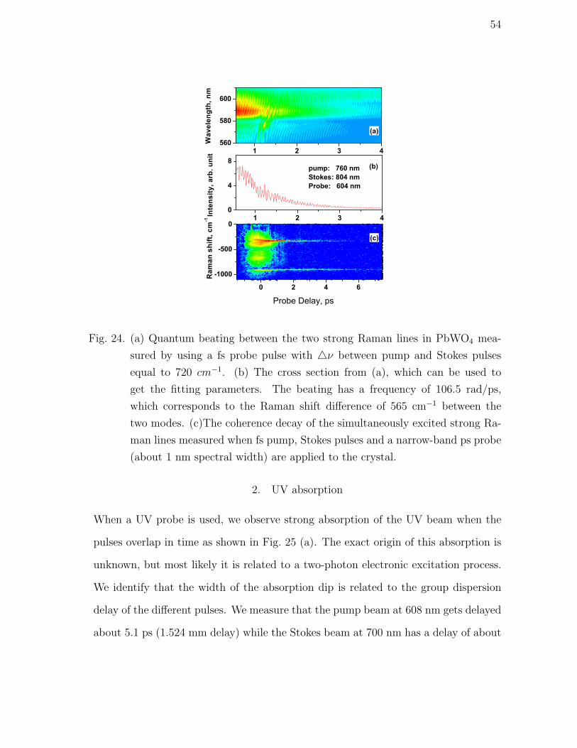
54

Fig. 24. (a) Quantum beating between the two strong Raman lines in PbWO4 mea-

sured by using a fs probe pulse with ν between pump and Stokes pulses

equal to 720 cm−1. (b) The cross section from (a), which can be used to

get the fitting parameters. The beating has a frequency of 106.5 rad/ps,

which corresponds to the Raman shift difference of 565 cm−1 between the

two modes. (c)The coherence decay of the simultaneously excited strong Ra-

man lines measured when fs pump, Stokes pulses and a narrow-band ps probe

(about 1 nm spectral width) are applied to the crystal.

2. UV absorption

When a UV probe is used, we observe strong absorption of the UV beam when the

pulses overlap in time as shown in Fig. 25 (a). The exact origin of this absorption is

unknown, but most likely it is related to a two-photon electronic excitation process.

We identify that the width of the absorption dip is related to the group dispersion

delay of the different pulses. We measure that the pump beam at 608 nm gets delayed

about 5.1 ps (1.524 mm delay) while the Stokes beam at 700 nm has a delay of about

55

Fig. 25. UV probe pulse intensity as a function of probe delay and pump delay. When

three beams overlap in time, the UV gets absorbed. (b) cross section of (a)

at a zero delay of the pump pulse. The dip width corresponds to the group

velocity delay of the pump and probe pulses. (c) CARS signal.

5.0 ps (1.494 mm). The UV beam at 350 nm experiences large dispersion which

results in a delay of 8.62 ps (2.586 mm). The difference is about 3.6 ps, which is

exactly the width of the dip we see in Fig. 25 (b). In Fig. 25 (c) we show that the

CARS signal starts at the front edge where the pulses begin to overlap and exhibits

quantum beating due to the simultaneously excited Raman modes.

3. The interference experiment

Next we investigate the mutual coherence among the generated sidebands. We first

generate multiple AS sidebands by focusing Red (λR= 718 nm) and IR (λIR= 812

56

nm) beams into the PbWO4 crystal. Then a third (Yellow) beam is sent along the

direction of the generated AS 3 sideband with a matching wavelength (λY = 574 nm).

Once the overlap in frequency, space, and time is achieved, the sidebands (AS 2 to

AS 7) start to visibly flicker, due to interference between signals generated through

different channels. We measure the pulse energy of AS 5 on a shot-by-shot basis by

using a fast photodiode.

Fig. 26. Histograms of AS 5 pulse energy. Solid black bars: the number of pulses (out

of 150) vs. AS 5 pulse energy generated with Red and IR input beams only.

White bars: the histogram of AS 5 pulse energy (913 pulses total) with the

addition of the third input beam. The dotted curve is a theoretical prediction

obtained assuming perfect single-shot coherence of the two interfering fields,

and random shot-to-shot variation of their relative phase.

The statistics of the AS 5 pulse energy is shown in Fig. 26. Solid black bars

give the histogram (number of pulses vs. AS 5 energy), with only Red and IR pulses

applied at the input. This histogram shows a typical normal distribution, with about

10% average variations. However, with the addition of the Yellow beam at the input,

the histogram of the AS 5 pulse energy (913 pulses total) transforms into a very

different distribution (Fig. 26, white bars). We perform a simple calculation, which

57

supports our qualitative understanding of this result. We consider interference of two

fields (of the same frequency), whose intensities (I1 and I2) fluctuate within 10% of

their mean values. We further assume that the relative phase of these two fields varies

randomly between 0 and 2π (every value of φ being equally probable). The resultant

intensity I = I1 + I2 + 2√I1I2[cos(φ)] is expected to produce a histogram that is

inversely proportional to the derivative of I with respect to φ and therefore has two

peaks (at I1+I2+2√I1I2 and I1+I2−2

√I1I2, where φ equals 0 and π respectively).

This is exactly what our simulation shows (Fig. 26, dotted curve). In this simulation,

we take the average value of < I1 >=0.41 (arbitrary units) from the measurement,

and find (from the best fit in Fig. 26) < I2 >=0.09. We repeat the calculation

91300 times (using random number generators), and divide the calculated number of

counts (per intensity) by a factor of 100 when we compare the simulation with the

experiment. The two peaks in the simulated histogram appear to be broadened by the

fluctuations of I1 and I2, which are taken to be 10% each (matching the experimental

observations). The peak on the right (at higher pulse energy) is calculated to be

lower and broader than the peak on the left, in excellent qualitative agreement with

the experimental data. This measurement, and its comparison with theory, confirms

our expectation that the (highly-coherent) Raman process results in generation of

mutually-coherent sidebands. We expect that if the phases of the input fields are

stabilized, the spectral phases at the output will also be stable.

F. Conclusion

In conclusion, we observe efficient generation of what to our knowledge is a record-

large number of spectra sidebands in Raman-active crystals driven by two-color fs

pulses. We observe sideband generation with excitation of either the Raman mode at

58

903 cm−1 or 325 cm−1. We find that phase matching plays a major role. The FWM

process and the Raman process coexist. The frequency spacing of the generated

sidebands is dependent on the angle and polarization of the beams. The generation

is optimized when the polarization of the two beams are parallel and when the angle

between them satisfies the phase matching condition.

More sidebands are generated when three beams are applied in a planar config-

uration when all three input beams lie in the same plane. When the three beams are

sent in a Box CARS configuration, a 2-D color array is generated. Different phase

matching conditions between the probe pulse and the the AS generated by the pump

and Stokes pulses result in a very different 2-D generation.

Using a third probe pulse, we observe absorption of the probe beam when a UV

probe is used. Also we measure the coherence decay time of the excited Raman modes

with both fs and ps probe pulses.

The generation in PbWO4 has low threshold and high converting efficiency. We

have measured up to 31 percent of the pump energy being converted to the sidebands.

The good temporal coherence implies that this broad-band light source may be used

for synthesis of subfemtosecond light waveforms.

59

CHAPTER IV

BROADBAND COHERENT LIGHT GENERATION IN DIAMOND USING TWO

OR THREE-COLOR FS LASER FIELDS

A. Introduction

In the last chapter, I describe the broadband generation in PbWO4 using fs pulses.

We also use another crystal diamond for the broadband generation. There are two

main reasons. Firstly, diamond has a single strong narrow Raman line at a very

large frequency shift (1332 cm−1), compared to the other crystals [64]. Because the

diamond sample exhibited one of the most intense Raman lines, the values of Raman

scattering cross section for the other materials that they investigated were normalized

to those of the diamond. They have shown, in this reference, that the integral Raman

scattering cross section determines the Raman gain coefficient in the transient case

[64]. Secondly, diamond is isotropic and the refractive index is well known, which

makes it easier (compared to PbWO4) to do some theoretical calculation and thus

help us understand the complicated experimental results.

Beside the above-mentioned two reasons, diamond also has several remarkable

properties which are desirable in our research [65]. First of all, diamond is capable of

transmitting an unusually broad spectral range (from x-ray region to the microwave

and mm wavelengths) and has the widest electromagnetic bandpass of any material.

There is an absorption band below 230 nm and an infrared absorbtion which lies be-

tween 1400 and 2350 cm−1. This broadband transmission is essential for the sideband

generation. It also makes diamond a good candidate material for far IR generation.

Secondly, it has an extremely high thermal conductivity (five times that of copper)

and is extremely chemically inert. Therefore, it is not easy to get damaged by laser

60

and does not require much protection from moist. At last, diamond has the highest

atom density of any material. A high density means a high Raman gain.

The well-known sharp Raman line, which corresponds to the energy of the triply

degenerate F2g vibrational mode of the two interpenetrating cubic sublattices of the

diamond [66], is used in the Raman spectroscopy to determine the bonding states of

the carbon atoms and to tell the diamond from the graphite-carbon-diamond aggre-

gates. The strong covalent carbon-carbon tetrahedrally bonding and light mass of

the carbon atoms result in a large frequency shift of the F2g optical mode. Back in

1963, diamond was chosen as a representative covalent crystal for the SRS experiment

and two S and 1 AS were observed when a high intensity (20 MW/cm2) Ruby laser

was used for excitation [67]. Later, the spectrum, gain, and angular distribution of

intensity of stimulated Raman emission in diamond was studied in detail [68]. They

found that the intensity of normal Stokes increased linearly with increasing laser in-

tensity up to the threshold for SRS, followed by a sharp increase in intensity by a

factor of 106 and eventually by saturation and damage to the crystal. Also the stim-

ulated linewidth was observed to be an order of magnitude narrower than the normal

linewidth. Natural diamond are costly and scarce. Recently, synthesis of large area

diamonds at lower pressure using chemical vapor deposition (CVD) technique was

developed. The quality of CVD diamond approaches that of the purest natural dia-

monds. The CVD diamond finds applications in laser physics such as heat spreaders

for high power laser diodes, optical components for CO2 lasers, UV detectors. Kamin-

skii et al. used CVD diamond for Raman laser converter based on SRS and reported

observation of SRS (up to 1 S and 3 AS sidebands) in diamond (using both ns and

ps pulses) [69; 66]. In this chapter we present the study of the Raman generation in

diamond using a pair of fs pulses.

61

B. Broadband coherent light generation in diamond driven by two-color femtosecond

laser field

Two input pulses

3o

5.8o

AS2

3o

5.8o

0.0

0.5

1.0

16000 20000 24000 28000 320000.0

0.5

1.0

800 700 600 500 400 300

Inte

nsity

, arb

. uni

t

Wavelength, nm

Frequency, cm-1

Fig. 27. The broadband generation in diamond with the two input beams (λ1= 630

nm and λ2= 584 nm, δν= 1250 cm−1) crossing at angles of 3 and 5.8.

Top: The generated beams are projected onto a white screen. The two pump

beams, S 1 and the first few AS beams are attenuated (after the sample) by a

neutral-density filter. The AS 2 spot clearly shows two different colors, with

blue corresponding to the Raman generation and green to the FWM signal.

Bottom: Normalized spectra of the generated sidebands.

First we apply two-color excitation in the diamond. The experimental setup is

about the same as the one we use for PbWO4 crystal. By applying two 50 fs pulses

(at λ1= 630 nm, λ2= 584 nm, and δν= 1250 cm−1), we obtain a generation of up to

16 AS and 2 S sidebands in a 0.5 mm thick diamond sample. The highest frequency

generated is in the UV region at a wavelength of 301 nm. Similar to the sideband

generation in PbWO4, the sideband doesn’t have a equally spaced frequency shift.

When we vary the crossing angle between the two applied laser beams (we used 3,

3.8, 4, 4.5 and 5.8), and record the changes in the generated spectrum (Fig. 27, only

62

3 and 5.8 are shown for clarity), we find that the generation is more efficient at a

3 beam crossing angle. The energy conversion from the pump beam to AS 1 is 3%.

It is 2% to the S1 and 0.5% to AS 2. The energy conversion from the pump beam

to all the sidebands is 14%. The generated sidebands using 3 crossing angle overlap

substantially in spectra with each other. Assuming that all the sidebands generated

from 3 crossing in diamond are properly phased or locked to each other, we estimate

that a single cycle of pulse with width of 0.5 fs can be obtained.

Fig. 28. The sideband frequency as a function of the sideband order (a) and as a

function of the sideband output angle (b) with the two input beams (λ1=630

nm and λ2=584 nm, δν= 1250 cm−1) crossing at two different angles, 3

(square) and 5.8 (round). The sidebands generated at 5.8 have a larger

(about twice) frequency spacing compared to the 3 case.

From Fig. 27, we can clearly see that the instantaneous FWM signal coexists with

Raman generation in the lower orders of the sidebands. The AS 2 beam spot shows

two colors: blue and green. By measuring the frequency shift from the preceding

sideband, we deduce that the blue is due to Raman generation, while the green beam

63

corresponds to the FWM signal.

Fig. 29. The Sideband frequency and output angle at the different detunings (ν vary

from 820 cm−1 to 2608 cm−1) between the pump (fixed at 594 nm) and Stokes

pulses. The output angles do not vary much, nor does the the frequencies of

the sidebands, although ν varies a lot.

We plot the sideband frequency versus the sideband order as shown in Fig. 28

(a). It shows that sidebands generated at 5.8 have a larger (about twice) frequency

spacing compared to the 3 case. Also the sidebands come out at a much larger

angle spacing as shown in the Fig. 28 (b) (we define the Stokes output angle as 0

degree). This is more obvious for low-order sidebands which are more affected by the

strong FWM signal. Both frequency and angular spacing decrease for the high-order

sidebands. This shows that the initial phase matching condition between the two

pump beams decides the generated sideband output angles and frequencies.

To prove that the sideband generation is from the Raman rather than the FWM

process, we keep the pump frequency the same while tuning the Stokes frequency

64

Fig. 30. The generation pictures and the pulse time responses in two different situa-

tions: (a) ν is tune close to resonance with the Raman transition and (b)

the Stokes and the pump wavelengths are phase-matched at the chosen an-

gle. When ν is on resonance with the Raman transition, the Stokes get

amplified.

from 820 cm−1 to 2608 cm−1 and record the sideband frequency. The result is shown

in Fig. 29. When ν varies from 820 cm−1 to 2608 cm−1, the output angle doesn’t

vary much. Also, the frequency vary much less compared to the change of ν. These

facts are clear indications that the signals are generated mainly through the Raman

process. The competing FWM process only affects the sideband slightly.

We always keep the laser intensity below the threshold for SPM. In diamond it

is 3.35 mW for the (yellow) pump beam and 0.822 mW for the (red) Stokes beam,

which are three to four times higher than the power used for PbWO4 crystal. As a

result, the effect of FWM on the sideband generation is more obvious compared to

that of the PbWO4. The generation is best in two situations. One is when ν=1074

65

cm−1, the frequency spacing is close to resonance with the Raman frequency. Now the

phase matching condition is poorly satisfied. Consequently, low-order sidebands are

relatively weaker. However, the high-order sidebands (from AS 6 to AS 9) are almost

equally strong and only get weak from AS 11, as shown in Fig. 30. Another situation

is when ν=2232 cm−1, the Stokes (at 680 nm) beam is in good phase matching

condition with the pump (at 594 nm) beam with the angle we choose. The low-order

sidebands are very strong because the boost from the FWM process. We conclude

that for optimal sideband generation, we should choose a pair of pulses which are on

resonance with the Raman transition and cross at an angle that satisfies the phase

matching condition.

Another interesting feature is the interaction of the pump and Stokes pulses at the

overlap (in time) region as shown in the bottom of Fig. 30. When ν is on resonance

with the Raman transition (λStokes=640 nm), the Stokes beam gets amplified through

the SRS process. That is to say, the intensity of the Stokes beam increases when the

pump field is present.

We see how the polarization of the pump and Stokes beams affects the sideband

generation in diamond through a different experiment than the one used for PbWO4.

When we vary the polarization of the Stokes beam relative to the pump beam, the in-

tensity of the sideband AS 1, AS 2 and AS 10 vary as shown in Fig. 31. The sidebands

have maxima when the pump and Stokes beams have parallel polarization (waveplate

angle at 0 or 180 degrees). No sidebands are generated when the polarization of the

pump and Stokes beam are perpendicular to each other.

66

Fig. 31. The intensity of the sideband AS 1, AS 2 and AS 10 as a function of the

polarization angle of the Stokes beam. The pump and the Stokes beams have

parallel polarization at 0 and 180 degrees.

C. Phase matching calculation

Due to the material dispersion, phase matching is optimized when different frequency

components propagate at different angles. To find out the optimal angle between a

pair of wavelengths we first do a simulation using the peak wavelengths of the pulses.

The refractive index of diamond is given by a generalized Cauchy dispersion

formula [70]:

n(λ) = 2.37 − 1.0 × 10−5/(1.24/λ)2 + 8.0 × 10−3 × (1.24/λ)2 + (4.1)

1.0 × 10−4 × (1.24/λ)4,

67

with λ in units of µm. This formula fits well with the available experimental data

[71; 65]. (Other constants which are related to our research is the third-order nonlinear

optical coefficient, which is 1.8 × 10−13 esu (2.0 × 10−22 m2/V2) and the nonlinear

refractive index, which is 1.3 × 10−15 cm2/W (it is one magnitude higher than that

of fused silica) [46]).

The k vectors for the pump and Stokes fields are:

kp =2 ∗ πλp

∗ n(λp) or simply in cm−1,

kp =104

λp∗ n(λp), (4.2)

kS =104

λS∗ n(λS).

Here p denotes for the pump field and S denotes the Stokes field (by convention,

ωp − ωS = ωRaman). From energy conservation, ωFWM = 2 ∗ ωp − ωs, we have

λFWM =2 ∗ π ∗ cωFWM

= 1/(2

λp− 1

λs), (4.3)

kFWM =104

λFWM

∗ n(λFWM). (4.4)

On the other hand, the optimal k vector can be calculated as :

Koptimal =√

(2kp cos θp − ks cos θs)2 + (2kp sin θp − ks sin θs)2. (4.5)

Note here the angle has to be converted to the angle inside the crystal by using the

Snell’s law.

We measure the wavelengthes (peak value) of the sidebands generated when the

crossing angle between the pump and Stokes beams is 3 . The results are shown

in table I. We then use a phase matching factor M=sinc2(δk ∗ L/2) to characterize

the phase mismatch between the input fields or the generated fields. δk = kFWM −

68

Koptimal, L is the sample thickness, which is about 500 µm in our experiment. When

we use the measured wavelengths and angles, we find that the sidebands are almost

perfectly phase matched (M is above 0.97 for the high-order sidebands).

Furthermore, we perform calculations that support our qualitative understanding

of the role of phase matching using a pulse instead of just the peak wavelength. We

take the spectral intensity of an n’s AS sideband as given by

In(ν) ∼ In−1(ν − νR) · sinc2[−→k (ν) −−→

k (ν − νR) −−→k R]L/2. (4.6)

Here−→k is the wavevector (k = nν/c), νR is the Raman shift and c is the speed of

light. The k-vector of the Raman excitation−→k R is determined by the directions of

the two input beams. We assume that the angle between the low-order sidebands is

approximately the same. From a simple phase-matching calculation as shown above,

the optimal generation of the lower-order AS sidebands is expected when the input

beams are crossed at a 3.6 angle.

We find that when the angle is smaller than the phase matching angle, the peak

frequency shift of the generated AS 1 from the pump pulse is 1163 cm−1, which is

smaller than the Raman shift and the opposite happens when an angle larger than

Table I. The wavelengths and the angles of the generated sidebands.

Stokes Pump AS1 AS2 AS3 AS4 AS5 AS6 AS7

λ (nm) 613.5 586 557.3 531.3 511.0 494.0 476.1 460.0 437.5

θ () 0 3.00 5.6 7.9 10.0 12.0 14.0 16.0 17.6

AS8 AS9 AS10 AS11 AS12 AS13 AS14 AS15 AS16

λ (nm) 423.5 407.48 394.7 385.1 375.1 366.9 358.6 351.8 345.0

θ () 19.1 20.5 22.0 23.6 24.9 26.4 27.8 29.2 30.5

69

Fig. 32. Theoretical calculation of the frequency of AS 1 when the two pump beams

(λS=630 nm, λp=581.23 nm, δν=1332 cm−1, exactly the Raman frequency)

cross at an angle of 2.6, 3.6 and 4.6 degrees, respectively. The phase matching

angle between the two input beams is 3.6 degrees. The sample thickness is

500 µm.

70

the phase matching angle is applied as shown in Fig. 32. The peak frequency shift of

the generated AS 1 from the pump pulse is 1301 cm−1 for a input angle of 3.6 degrees

and 1466 cm−1 for 4.6 degrees. This agrees with our experimental observations on

diamond. The peak wavelengths of the two input pulses phase-matches at 3.6 degrees.

Therefore, when the two input pulses cross at 5.8 degrees, the generated spectrum

has a larger frequency spacing than that of the 3 degrees. This calculation may also

explain the gradually decreasing frequency spacing between the sidebands, since the

optimum beam-crossing angle increases with a increasing sideband frequency because

of the normal medium dispersion.

Fig. 33. The sideband generation in diamond at the different delays between the two

pump pulses (λ1= 630 nm and λ2= 584 nm, δν= 1250 cm−1). The time delay

between each picture is about 20 fs. We see at certain delays, the high-order

sidebands are brighter than the lower ones.

Raman generation in crystal is a complicated process. For example, we observe

that the sideband intensity varies as we vary the delay between the two pulses. We

have observed that high-order sidebands have higher intensity than the lower order

ones as shown in Fig. 33, counter-intuitively. We guess that this is due to the phase-

matching condition for the sidebands since the intensity of the radiation generated

71

by FWM is given by [72]:

I =9ω2

s

16c4ε20nsnSn

2p

|χ3FWM |2l2IiI2

p sinc2(kl/2). (4.7)

Here ωs is the signal frequency, ns, nS, np are the refractive indices for the signal,

Stokes and pump beams, respectively. The phase-matching factor sinc2(kl/2) may

modulate the sideband intensity.

D. Coherence between the sidebands

YellowIR Green (M easured)Red

0 1 2

0

1

2

3

4

Intensity, arb. unit

Tim e, ns

Fig. 34. “Green” sideband energy under different conditions. Black solid line: all

three input pulses are present. Red dotted line: IR and Red pulses present

only. Green dashed line: Yellow and Red pulses present only. Top: the input

beam geometry.

We test the mutual coherence among the generated sidebands through an inter-

ference measurement. We use three input beams (instead of two) and align them in

one plane, such that the higher-order AS sidebands generated through different chan-

nels overlap in space. We first generate AS 2 (Green, λGreen= 545 nm) by focusing

Red (λR= 690 nm) and IR (λIR= 802 nm) pulses into the diamond crystal. Then

72

we send a third beam in the direction of the generated AS 1 beam, as shown in Fig.

34(top). We tune the frequency of this third applied field (Yellow, λY ellow= 590 nm)

such that the AS 1 generated from Red and Yellow fields coincides (both in space

and frequency) with the AS 2 generated by Red and IR pulses. νGreen − νY ellow=

1400 cm−1, which agrees well with the Raman shift of 1332 cm−1. When only one

pair of pulses (either one) is applied to the crystal, the energy of the combined field

(measured with a photodiode) is about 1 unit. When all three pulses are applied, the

measured energy varies from 0 to 4 units from shot to shot as shown in Fig. 34 (we

show 9 random shots), as a result of coherent addition of the two generated pulses.

Since we don’t attempt to stabilize the phases of the three input fields, the interfer-

ence of the generated “Green” pulses is partially constructive or destructive, at ran-

dom. We conclude that the two pulses, generated through the two separated Raman

processes, have good mutual coherence. This measurement confirms our expectation

that the (highly-coherent) Raman process results in generation of mutually-coherent

sidebands. Assuming that all the sidebands generated from 3 crossing in diamond

are properly phased or locked to each other, we estimate that a single cycle of pulse

with width of 0.5 fs can be obtained.

E. The measurement of the coherence decay time of the CARS/CSRS signals

The unequal frequency spacing between the generated sidebands raises the question of

the purity of the diamond we use. Using a pair of visible pulse as the pump (584 nm)

and Stokes (635 nm) while using a UV pulse (318 nm) as a probe pules, we observe

the CARS signal at 305.8 nm (δν= 1250 cm−1) and CSRS signal at 332 nm (δν= 1326

cm−1) (Fig. 35). Undoubtedly, this is the strong Raman line in diamond. The width

of the line in the SRS spectrum ∆νR is about 2.5 cm−1. Accordingly the phonon

73

Fig. 35. The CARS and CSRS signals observed in diamond using a UV probe pulse.

Top, the spectra of the CARS (left, center wavelength is 305 nm) and CSRS

(right, center wavelength is 332 nm) as a function of the probe delay. Bottom,

the exponential decay time of the CARS (left) and CSRS (right) signals.

relaxation time is T2 = (πc∆νR)−1 ≈4.2 ps [69]. We measure the exponential decay

of the the CARS/CSRS signals as shown in Fig. 35. Using ICARS ∼ A exp(−t/T2),

with A a constant, we obtain a decay time (T2) of 2.6 ps for the CARS signal and 2.7

ps for the CSRS signal. This corresponds to a 4 cm−1 linewidth. The deviation could

be due to the use of fs pulses. We also measure that AS 2 has a exponential decay

with T2=1.47 ps, which is half that of the AS 1. There is an obvious gap (about 1.5

ps) from the FWM signal to the CARS peak, which remains another mystery to us.

74

Fig. 36. The 2-D array generation in diamond with three input pulses (λpump= 720

nm, λStokes= 800 nm, and λprobe= 600 nm). The wavelengths of the sidebands

are labelled in nm. The degenerate FWM signal (2Y-IR, a shorthand of

2ωY − ωIR) from the probe and Stokes pulses and the one (2Y-R) from the

probe and pump pulses are much stronger than the Raman generation spots.

They either superimpose or shift slightly. The six-wave-mixing signal (3Y-2R)

from the pump and probe pulses is also visible.

F. Two dimensional color array generation in diamond driven by three-color fem-

tosecond laser field

Similar to PbWO4, when we apply a Stokes pulse (IR, 800 nm), a pump pulse (red,

728 nm) and a visible probe pulse (yellow, 600 nm) at the usual Box CARS geometry,

in addition to the strong CARS and CSRS signals, we obtain a 2-D color array as

shown in Fig. 36. Here the angle between the pump and Stokes beams is 5 degrees.

The probe beam is 11 degree from the pump beam and 16 degrees from the Stokes

beam. Due to a different dispersion from that of the PbWO4, the generated 2-D color

array is very different although same input angles between the beams are used. In

addition, with a single Raman line, the result is easier to understand. The frequency

spacing between the pump and Stokes pulses is around 1000 cm−1. As a result, the

75

average sideband spacing is very regular, about 1040 cm−1. The sidebands in the first

row are generated by the pump and Stokes pulses. The second row is generated by the

CARS/CSRS and the high-order CARS processes. The FWM signal from the probe

and Stokes/pump pulses leads generation of the third row. The degenerate FWM

signal from the probe and Stokes pulses (2ωY − ωIR) and from the probe and pump

(2ωY − ωR) pulses are much stronger than the generation spots due to Raman effect.

They either superimpose or shift slightly. The six-wave-mixing signal (3ωY − 2ωR)

from the pump and probe pulses results in the fourth row sideband generation. We

measure the coherence decay time again so that we can compare it with that measured

with a UV probe beam. The CARS signal (558.6 nm) has a frequency shift of 1235

cm−1 from the probe pulse and an exponential decay of 2.5 ps. The CSRS signal

(652.2 nm) has a frequency shift of 1329 cm−1 and an exponential decay of 3.0 ps.

These decay times are similar to the ones obtained with a UV probe pulse. Similar

to the situation in which a UV probe pulse is used, the CARS frequency shift is

somehow smaller than the CSRS frequency shift from the pump pulse. If we look at

the phonon dispersion curve of diamond [73], there is a peak at 1040 cm−1. This peak

may explain the frequency shift of 1040 cm−1.

G. Conclusion

We show that beside PbWO4, broadband generation using diamond is also possible.

Nonlinear frequency conversion in diamond is efficient. We have measured 7% energy

conversion into the AS 1 and 1% into the AS 2 and S 1. The high-order CARS/CSRS

and FWM/SWM signals are also observed in the crystal. From the theoretical cal-

culation we find that when the angle between the pump and Stokes beams is smaller

than the optimal phase matching angle, the frequency spacing between the sidebands

76

is smaller than the Raman shift and the opposite happens when the angle between

the pump and Stokes beams is larger than the optimal phase matching angle. It may

explain the frequency spacing decreases for the high-order sidebands as well. We also

study the coherence decay of the Raman mode using the fs pulses. Similar to PbWO4,

we observe a 2-D color array generated when three-color fs laser beams are applied in

the diamond in a Box CARS geometry. Due to a different dispersion, the 2-D color

array is very different from the one generated in PbWO4 under the same input beam

conditions.

Compared to PbWO4, we find that the onset of the SPM in diamond starts at

a higher intensity of the laser pulse. Therefore a higher energy pulse can be used.

However, the threshold for the Raman generation is higher too. The beams are more

affected by the FWM process so that multiple peaks often show up in the low-order

sidebands. As a result, the sideband spectrum is not as clean as that of the sideband

generated in PbWO4.

We believe that the generation can be optimized by choosing a pair of beams

with proper wavelengths and using a lens with an optimal focal lens so that the beams

cross at the crystal with a phase matching angle. Also smaller dispersion means that

the generated sidebands can be increased both in number and energy by using a

thicker sample (say, 1 mm), since more Raman gain can be obtained.

77

CHAPTER V

BROADBAND GENERATION IN RAMAN CRYSTAL DRIVEN BY A PAIR OF

TIME-DELAYED LINEARLY CHIRPED PULSES

A. Introduction

In chapter III I present the results of sideband generation in the PbWO4 crystal by

focusing two near transform limited 50 fs laser pulses to the sample [74]. However,

limited by the SPM and other nonlinear parasitic processes, at most 2 to 3 mW power

can be used before the pulses get distorted. In this chapter, we study experimentally

the broadband generation in the PbWO4 crystal driven by a pair of time-delayed

linearly chirped pulses (pulse duration ranges from 100 fs to 2 ps).

A pulse is called linearly chirped when its phase has a quadratic variation, i.e., the

instantaneous frequency varies linearly with time delay. The frequency of a negatively

chirped pulse decreases as a function of time delay, while the frequency of a positively

chirped pulse increases vs. time. A transform limited fs pulse excites all the Raman-

active modes accessible by the pulse width, as have been shown in the chapter III. For

a pair of linearly chirped pulses, the difference between the instantaneous frequencies

depends only on the time delay. When the frequency difference equals to a Raman

frequency, this mode can be selectively excited [35]. In the time domain, a periodic

pulse train is created, with a period equals to the period of a single Raman vibrational

mode, as will be shown later in the theory section. A simplified setup for high-

resolution spectroscopy has been built using a pair of time-shifted, linearly chirped

pulses [75]. A related method of achieving the spectral selectivity is Fourier domain

pulse shaping, when a pulse train is created by applying a periodic spectral phase to

a single fs pulse using a pulse shaper [76].

78

Fig. 37. Schematic of the experimental setup. VF: Variable neutral density filter; BS:

50/50 ultrafast beam splitter. An approximately linearly chirped pulse is

obtained by misalignment of the compressor in the amplifier. It is split into

two and later recombined at the sample with a relative time delay.

We present and discuss the different sideband generations obtained through the

different Raman mode excitations by varying the time delay and the crossing angle

between the two pump beams. The sideband generation by the excitation of Raman

line at 325 cm −1 is compared to that of using two-color near transform limited fs

pulses with a central frequency separation close to the Raman frequency.

B. Experimental setup

The experimental setup is shown in Fig. 37. Briefly, the output of the regenerative

amplifier (Legend, Coherent) is an infrared beam (λ=802 nm) of 35 to 50 fs pulses

with a 1 kHz repetition rate and 1 W average power. It is split into two by an ultrafast

beamsplitter. The delay between the two pulses can be varied by moving (with an

electronic motion controller) a retro reflector which is mounted on a delay stage. The

two beams are recombined and focused in the crystal by a 2 inch focal lens (f=50

cm). Both beams are attenuated by two variable neutral density filters so that the

79

Fig. 38. Schematic of a compact compressor. Adapted from the laser training material,

Coherent.

power used is below the threshold of the onset of the parasitic nonlinear processes.

The power used ranges from 5 mW to 20 mW, depending on the pulse chirp rate and

the focusing condition.

A schematic drawing of a compact compressor with a folded geometry is shown

in Fig. 38. Normally two gratings are needed. Here the roof-mirror reflects the

beam back to the same grating (different part) so only one grating is used. A long

pulse with a time chirp is compressed after the compressor to a short pulse with no

chirp. The roof-mirror is mounted on a translation stage that can be adjusted using a

controller. Moving of the roof-mirror results in the changing of the effective distance

between the gratings, therefore the changing of the chirp of the output pulse, as is

shown in the theory part. The zero delay between the two pump pulses can be found

by focusing the two beams (unchirped pulses) at a very small (less than 2 degrees)

crossing angle in a piece of glass. When the two beams overlap both in space and

time, an interference pattern around the two pump beams can be easily seen by the

eye when they are projected to a paper screen after the crystal. Several orders of

self diffraction (SD) of the beam can be seen when enough power is applied. The SD

80

signals show up symmetrically beside the two pump beams, similar to the picture as

shown in Fig. 39 (c) (figure on page 82). The first order SD signal by the pump beam

with a variable delay is what we used to measure the chirp introduced, as shown

in Fig. 39 (b) (figure on page 82). We can see that the pulse we used is negatively

chirped, with a pulse duration (FWHM) ranging from 80 fs to 2 ps. The chirp is

approximately linear. The narrowing of the spectrum on the top (longer wavelength)

might be due to the measuring range of the fiber-coupled spectrometer, which cuts

off at wavelength 870 nm. The SD signals in crystal are much stronger compared to

that in glass.

C. Theory

In this section I show how to estimate the chirp introduced to a pulse by changing the

effective distance between the two gratings, and how to use the relationship between

the time delay and the pulse chirp to identify which Raman mode is excited. I also

show how a periodic pulse train resonantly excites the molecular vibrations, which

lead to the sideband generation in the crystal.

1. Chirped pulse characterization

The temporally chirped pulse width introduced by moving the distance l between the

gratings is [77]:

δλτ =l(λ/d)δλ

cd[1 − (λ/d− sin γ)2]. (5.1)

where δλτ is the variation of group delay, l is the slant distance between the gratings,

d is the grating constant, δλ is the bandwidth of the pulse, c is the speed of light,

and γ is the angle of incidence. In our experiment, λ=802 nm, δλ=35 nm, d−1=1500

lines/mm, and γ is about 30. When plug in these numbers we get: δλτ= 4.2 l ps/cm.

81

In terms of frequency ω (=2πc/λ), the group delay can be expressed as:

δωτ =−4π2clδω

ω3d2[1 − (λ/d− sin γ)2]. (5.2)

Thus the linear relation between the delay and the frequency can be expressed as

[77]:

τ = τ0 − ω − ω0

µ+O(ω − ω0)

2. (5.3)

Here µ−1 = −4π2clω3d2[1−(λ/d−sin γ)2]

, which is proportional to l. Therefore ∆τ = td = ∆ω/µ.

For a fixed ∆ω=ωR, td is proportional to l, so the slope of td vs. the chirp rate is

proportional to the Raman frequency ωR.

The sideband generation in crystal is strongly influenced by the phase matching

and thus the sidebands have a non-equal frequency spacing (decreasing for high-

order sidebands). This relationship between the td and ωR can be used to identify

which Raman mode is excited. For example, one possible Raman mode which can be

confused with the Raman mode at 903 cm−1 is one at 762 cm−1. The intensity of this

line is around 50 times lower than that of 903 line. However, the pulse intensity at

762 cm−1 width is 3 times higher. Raman generation is a highly non-linear effect so

it is possible that 762 cm−1 can dominate. We measure td using different chirp rate

pulses with the crossing angle between the two pump beams varying a few degrees.

With a small angle crossing, only the 325 cm−1 Raman is excited so we can use the

slope of the td vs. the different chirp rates as a reference slope. We measure a slope of

0.01 for a small angle crossing between the two pump beams and 0.028 for a relatively

larger angle (4 degrees). Therefore we get ωR2/ωR1 = 2.8, which is exactly the ratio

between the 903 cm−1 and 325 cm−1. So we identify that the strong Raman mode

903 cm−1 is excited at a large angle, not the one at 762 cm−1.

We change the chirp gradually by a controller. Using the SD-FROG method

82

760

800

840

Wav

elen

gth,

nm

-2 -1 0 1-2 -1 0 1760

800

840

IR Delay, ps

R

Time Delay

Movable by delay stage

(a)(b)

(c)

0.08 ps 0.2 ps

1.72 ps0.62 ps

Fixed pump Movable pump

Fig. 39. (a) The schematics of the pulses for the Raman excitation; (b) The chirp of

the pulses measured with SD-FROG; (c) Multiple orders of the self diffraction

signals in the crystal.

and assuming a linear chirp, we measure a chirp rate of 1281 cm−1/ps, 620 cm−1/ps,

and 319 cm−1/ps respectively (Fig. 39 (b)). We then calculate the chirp rate b

from b=ωR/(2td) by measuring the td using pulses with different chirp rate when the

Raman mode at 325 cm−1 is excited. We find these chirp rate agree well with our

direct measurements using the SD-FROG method, which justifies our assumption of

linear chirp.

2. Coherence preparation

A linearly chirped pulse can be written as:

E(t) = exp(−at2) ∗ exp[I ∗ (bt2 + ωlt)]. (5.4)

Here 1/√a is roughly the pulse duration, b is the chirp rate of the pulse, and ωl is

the laser frequency.

83

The intensity for two time-delayed linearly chirped pulses is:

I(t) = |E(t) + E(t− td)|2 (5.5)

= exp(−2at2) + exp[−2a(t− td)2]

+ 2 exp[−a(t2 + (t− td)2] cos[b(2t− td)td + ωltd].

When ∆ω=ωR=2btd, the last term in It is proportional to cos(ωRt+C) (C = (2ωlωR−ω2R)/4b, is a constant). We see that there is a periodic beat in the pulse intensity in

the time domain. The periodicity of this pulse train can be matched to the period of

this Raman mode at ωR, permitting selective mode excitation [75]. One can adjust

the excitation frequency simply by adjusting the time delay between the two pulses.

Molecular vibrations resonantly excited by a periodic sequence of short pulses has

been described in detail by Gershgoren et al. [75] and Zheltikov [35]. The impulsively

stimulated Raman scattering can be described by a driven damped harmonic oscillator

[35]:

d2Q

dt2+ 2Γ

dQ

dt+ Ω2Q = F (t), (5.6)

where Ω is the Raman frequency and Γ is the relevant damping rate, and F(t) is the

external force applied. When a pulse train is used, the amplitude of the molecular

vibrations is [35]:

Q(t) =C

Ω

sin πNTT0

sin πTT0

sin(Ωt+ ϕ), ϕ = πT

T0

(N − 1), (5.7)

here T0 = 2π/Ω, N is the total number of pulses in the pulse sequence, C is a

constant. We can see that when T is a multiple integer of the period of the molecular

vibrations T0, the amplitude of the molecular vibrations has a maximum. As a result

of the coherently excited molecular vibrations, many sidebands can be generated, as

84

described in chapter II.

D. Experimental results and discussion

We have shown in the earlier chapters that the angle between the two pump beams is

very critical for generation in Raman crystals. For example, to effectively excite the

903 cm−1 Raman mode, an angle of 3 to 4 is needed. While for the lower frequency

Raman mode at 325 cm−1 to be excited, a smaller angle 2.5 works the best. We

vary the the angle by adding a 20 cm negative lens after the 50 cm lens with a proper

distance. Next we discuss the sideband generation at the different crossing angles

between the two pump beams. For convenience of description, I call the pump beam

which delay can be varied as the movable pump and the other one as the fixed pump

beam.

1. Self diffraction and the excitation of the Raman mode at 191 cm−1

When the angle between the two pumps is around 1, self diffraction of the beam is

observed at 0 delay as shown in Fig. 39 (c). Here we use collimated beams which

have a beam size of about 1 mm.

When we apply a pair of linearly chirped pulses with a chirp rate of 2100 cm−1/ps

to the crystal, we observe up to 40 AS and 5 S sidebands generated as shown in Fig. 40

(a). The angle between the two beams is about 1.2. We first observe AS generation

on the movable pump side at delay td (here the movable pump acts as the pump

beam and the fixed pump as the Stokes beam, as conventionally ωp > ωs.). When we

move the pulse forward from 0 delay to -td, we observe generation on the fixed delay

side. Now the fixed pump functions as a pump beam. Here only the picture in one

side is shown since the generation pictures in both sides are symmetric. Due to the

85

loose focus of the beam, both the pump and the Stokes power is higher than 5 mW

when measured after the crystal. The conversion efficiency from the pump beam to

the sidebands is 25 %. The conversion efficiency of Stokes beam is about the same.

Fig. 40. Broadband generation in a PbWO4 crystal using two time-delayed linearly

chirped pulses applied at an angle of 1.2 to each other. The chirp rate of the

pulse is about 2100 cm−1/ps. (a) Generated beams projected onto a white

screen. (b) Normalized spectra of the generated sidebands from AS 11 to

AS 37. The wavelength is in reciprocal scale. (c) The peak frequency of the

generated sideband plotted as a function of the sideband order. Multiple value

corresponds to the multiple peaks in the sideband spectrum. The high-order

sidebands have a slope of 200 cm−1 per AS order.

The spectra of the high-order sidebands (AS 11 to AS 37) are shown in Fig. 40 (b).

There is substantial overlap between the spectra of the generated sidebands. When

the angle is smaller and therefore a lower frequency Raman transition is excited,

we observe continuum generation instead of the distinctive spots for the high-order

86

sidebands, due to the small angle separation and the wide spectrum of the sideband,

similar to the picture shown in Fig. 41 (a). In Fig. 40 (c) we plot all the sideband

peak frequency as a function of the sideband order. Here the multiple values means

multiple peaks in spectrum. The average frequency spacing of the sidebands is around

200 cm−1. We believe the generation at this angle is due to the excitation of Raman

line at 191 cm−1. The slight bending of the slope indicting a decrease in the frequency

spacing.

2. The excitation of the Raman mode at 325 cm−1

When two color excitation is used and the angle between the two pumps is small,

we observe generation due to 320 cm−1 Raman mode excitation. About 30 AS is

observed as shown in Fig. 41 (a). Only 2 to 3 mW power can be used, limited by the

onset of the SPM. This mode should be easily accessed by the chirped pulse since the

width (FWHM) of the pulse is around 460 cm−1. To observe this, we use one 2 inch

lens with focal length of 50 cm. The angle between the pumps is about 2.4 . As

many as 40 AS have been observed at two different delays. The output angle of the

highest sideband with respect to the pump is about 50 . Counterintuitively, like in

diamond, we again observe that some of the high-order sideband is stronger than the

low-order ones, as shown in Fig. 41 (d). This can be seen more clearly when a large

angle between the two pump beams is used. There are two possible explanations.

One is that the FWM coexist with the Raman process. When a certain order of the

two processes is overlapped, that signal gets enhanced. A proof is that the sideband

generation pattern changes when we vary the delay, since FWM signal varies as

the delay changes. The other explanation is that the phase matching factor somehow

modulates the intensity of the output sidebands, as described the last chapter. Further

theoretical investigation is needed to solve this “mystery”.

87

Fig. 41. (a) Broadband generation in PbWO4 crystal pumped by fs pulses (λS=804

nm, λS=766 nm, and ν= 617 cm−1). The angle between the pump and

Stokes beam is 2.9 . A third probe pulse (Y) leads to generation of many

orders of CARS and CSRS signals. (b) Broadband generation in a PbWO4

crystal using two time-delayed linearly chirped pulses applied at an angle of

2.4 to each other. The chirp of the pulse is about 2100 cm−1/ps. (c) The

generated beams by using a pair of linearly chirped pulses with a large chirp

rate, 440 cm−1/ps. d) The intensity modulation of the generated sidebands.

The generation at a chirp rate of 2100 cm−1/ps is shown in Fig. 41 (b). We

observe 40 AS and 3 S sidebands. The spacing between the sidebands is around 320

cm−1 in average. It decreases to 240 cm−1 for the high-order sidebands. As high

as 41 % conversion efficiency has been measured for the pump beam and 21 % for

the Stokes beam. When the chirp rate is increased to 1060 cm−1/ps, the sideband

generation seems less effective. The AS number decreases to 34. The pump beam

has a 33 % conversion efficiency and the Stokes bean 19 %. When we introduce more

chirp until a chirp rate of 440 cm−1/ps is reached, the efficiency reduces to about

14 % for the pump beam and 11 % for the Stokes beam. About 22 AS is observed.

88

However, the absolute input power can be increased to 15 mW without introducing

the nonlinear parasitic effects. Another feature of the generation using pulses with

a high chirp rate is that the FWM signal gets weaker. Consequently, the generated

sidebands have good beam profiles and the spectrum is mostly single peaked, as shown

in Fig. 41 (c).

Fig. 42. Comparison of the sideband generation in PbWO4 crystal using two near

transform limited fs pulses (δν=615 cm−1) and a pair of time-delayed chirped

pulses. Many more sidebands are generated in the latter case.

In Fig. 42 we plot the sideband frequency as a function of the sideband order.

The square ones are the CARS/CSRS signals generated by all three beams when fs

pulses are used (Fig. 41 (a), top row). The probe beam (Yellow) is labelled as 0

order. The frequency spacing is regular, about 345 cm−1 per AS order. Compared

to the sidebands generated by two fs pulses (Fig. 42, round dots), there are many

more sidebands generated when a pair of time delayed linearly chirped pulses are used

(Fig. 42, triangles). The AS sidebands covering a range of 12,000 cm−1 span.

89

3. The excitation of the Raman mode at 903 cm−1

The Raman mode 903 cm−1 frequency is the strongest Raman mode in the PbWO4

crystal. The FWHM of the pulse we used is around 400 to 500 cm−1, depending on

whether the iris is fully open or not. To find out this chirped pulse excitation can be

used for this Raman mode, we change the angle between the two pumps to about 4.

We observe generation up to 15 AS as shown in Fig. 43.

Fig. 43. Sideband generation in a PbWO4 crystal using two time-delayed linearly

chirped pulses applied at an angle of 4 to each other. The chirp of the

pulse is about 620 cm−1/ps. (a) Generated beams projected onto a white

screen. Pictures are taken at three consecutive time delays between the two

pump beams, with a increase of 33.3 fs. (b) The picture of the high-order

sidebands. They are brighter than the low-order sidebands. (c) Normalized

spectra of the two pump beam and the generated sidebands (left) and the

peak sideband frequency plotted as a function of the sideband order (right).

The slope is around 540 cm−1 per AS order.

90

With a large angle, the non-resonant FWM signal is more separated from the

Raman generation as shown in Fig. 43 (a). We show the sideband generation picture

at three consecutive time delays between the two pump beams, with a separation of

33.33 fs. As we can see, the large spot, which is due to FWM generation process,

shifts as the delay varies. When certain order (circled by dots in Fig. 43 (a)) overlaps

with the Raman generation (small round spot), the intensity of that order enhanced.

When lower power or higher chirp rate pulses are used, the FWM process weakens

and only sidebands generated through Raman processes appear. When high power or

less chirped pulses are used, this FWM process sometimes leads to the distorted beam

profile of the lower orders due to the competition between the two processes as shown

in Fig. 43 (b). However, the high-order sidebands have good beam profiles. The

spectra of the two pump beams and the generated sidebands are shown in Fig. 43

(c). The frequency spacing between the sidebands is decreasing from low-order to

high-order sidebands, similar to the situation of sideband generation using two-color

fs excitation. When we plot the peak frequency of the sideband as a function of the

sideband order, we see a linear slope with a 540 cm−1 per AS order, which is much

smaller than 903 cm−1. The reason could be that this mode can only be excited by

the edge of the chirped pulses.

E. Conclusion

We shape a fs pulse by introducing a linear chirp so that the pulse duration is close

to the coherence life time in solids. The pulse is split into two and recombined on

the crystal with a relative time delay. We adjust the time delay between the two

pulses so that the difference of the instantaneous frequencies equals to a certain Ra-

man frequency. As expected, this Raman mode is selectively excited and substantial

91

coherence builds up in the crystal. We measure up to 40 AS and 5 S sidebands gen-

erated. The conversion efficiency from the two pump beams to the sidebands is very

high, for example, we have measured as high as 41 % conversion efficiency for the

pump beam and 21 % of for the Stokes beam. By compare the sideband generation

using the pulses with different chirps, we show that the nonlinear parasitic effect can

be avoided by using a more chirped pulse. Thus laser pulses with more power can be

used for the Raman excitation. However, if the peak intensity of the pulse is too low,

the sideband generation is not very efficient either, as can be seen from the decrease

in the conversion efficiency of the pump beams.

Compared to the two-color fs pulses excitation, this method has the advantage

of more sideband generation (the AS sidebands covers a range of 12,000 cm−1 span),

high conversion efficiency, high input power allowed (the power can be used without

creating the parasitic nonlinear effect such as SPM can be 10 times higher than the

transform limited pulse power used), and simpler setup. Although the FWM process

still creates some multiple peaks structure in the spectra of the low-order sidebands,

the complication due to simultaneous multiple Raman lines excitation when fs pulses

are used is eliminated. Different Raman mode can be selectively excited by varying

the time delay and the angle between the two pump beams.

This experiment confirm again that the phase matching condition plays an im-

portant role in the Raman generation process in crystal. When we vary time delay

between the two pulses, no sideband generation related to Raman mode at 903 cm−1

is observed when the crossing angle between the two pump beams is small. On the

other hand, at large angle, no sideband generation related to the Raman mode at 325

cm−1 is observed either.

The generation is more efficient for excitation of low frequency Raman mode at

325 cm−1 than that of high frequency mode at 903 cm−1, which can be only excited

92

by the edge of the chirped pulses. We believe that if a two separately prepared time-

delayed linearly chirped pulses which have a frequency difference of 903 cm−1 can be

used, the sideband generation should be very efficient.

Since the generation is very sensitive to the time delay, this method can be used

to measure the chirp when the Raman frequency is known or the other way around.

This broadband generation can also be used for a continuum generation or a tunable

light source. Most important of all, we have shown previously that the sidebands

generated are mutually coherent [74]. Therefore it opens a possibility for this broad-

band light source to be used to synthesize subfemtosecond light waveforms.

93

CHAPTER VI

FEMTOSECOND COHERENT ANTI-STOKES RAMAN SCATTERING

APPLIED TO THE DETECTION OF BACTERIAL ENDOSPORES∗

A. Introduction

Dipicolinic acid (DPA) is a marker molecule for bacterial spores [43] and the ability

to detect trace amounts of it is of paramount importance. We work with DPA in a

H2O/NaOH solution (NaDPA). Optical coherence of NaDPA has a relaxation time of

the order of 30 fs, and vibrational coherence in liquids typically has a picosecond life

time. Femtosecond pulses therefore are essential for the study of a complex organic

molecule such as NaDPA. Impulsive pump-Stokes excitation (the pulse duration is

shorter than the molecules vibrational beat cycle) of multiple modes of molecular

vibrations results in quantum beats in the signal, which facilitates unambiguous de-

tection of a target species and its discrimination against interferents [78]. These ob-

servable quantum beats, which allow extraction of species-specific parameters, occur

on a subpicosecond time scale and therefore require femtosecond probing. For exam-

ple, we have utilized fs CARS to study the vibrational dynamics of methanol-water

solutions by measuring the beat frequencies between Raman modes and coherence

decay rates of C-H stretch modes (at 2835 cm−1 and 2943 cm−1) in methanol [63].

∗Part of this chapter is reprinted from “Concentration dependence of femtosecondcoherent anti-Stokes Raman scattering in the presence of strong absorption,” by M.Zhi, D. Pestov, X. Wang, R. K. Murawski, Y. V. Rostovtsev, Z. E. Sariyanni, V. A.Sautenkov, N. G. Kalugin, and A. V. Sokolov, 2007, J. Opt. Soc. Am. B, 24, 1181-1186 (2007), copyright 2007, with kind permission from Optical Society of America.

94

B. Concentration dependence of femtosecond coherent anti-Stokes Raman scattering

in the presence of strong absorption

Theory suggests that the CARS generation efficiency can be increased by using elec-

tronically resonant pulses. We have shown that when a UV probe pulse with a

frequency near resonant to the first excited electronic state of the molecule is used,

the efficiency per particle is 20-fold higher compared with a nonresonant probe pulse

[79]. In such a near-resonant configuration, absorption is intrinsically present and

limits signal generation at large concentrations. The propagation of ultrashort pulses

through resonant media has previously been studied in both linear [80] and nonlin-

ear regimes [81]. However, these previous results do not directly apply to the present

work since our pulse spectrum is substantially narrower than the UV absorption band

of DPA, which has a peak at 272 nm (see Ref. [82] or Figure on page 151).

In this section we present a detailed study of the concentration dependence of the

CARS and CSRS signals. In particular, we have observed slopes having as large as

the third power of concentration. We present a model that describes the propagation

of the generated signal through the attenuating medium that agrees with our exper-

imental results. We have derived an analytic expression for the signal intensity that

includes a concentration-dependent dispersion. This generalized solution properly

describes the observed deviations from the quadratic density dependence.

1. Experimental setup

The experimental setup is shown in Fig. 44. Briefly, the output of the regenerative

amplifier (Legend, Coherent) is an infrared beam of 40-50 fs pulses with a 1 kHz

repetition rate and 1 W average power. A small fraction is used as the Stokes beam

(λStokes = 806 nm). Approximately 60% of the infrared power is sent into optical

95

parametric amplifier (OPA) 1 (OPerA-VIS/UV, Coherent), which provides the pump

pulses at λpump = 726 nm. The rest is used by OPA 2 (OPerA-SFG/UV, Coherent)

to generate the probe beam (λprobe = 295 nm). The pump and Stokes beams have a

few milliwatts of average power on the sample. The UV probe power is ∼0.5 mW.

The sample is a NaDPA solution in a 100 µm quartz cell. After spatial separation,

the generated beam is focused on the entrance slit of the monochromator (MicroHR,

Jobin Yvon), which has a liquid-nitrogen-cooled CCD camera (Spec-10, Princeton

Instruments) attached to the exit.

Pum

p

Osc

illat

orA

mpl

ifier

OPA 1 OPA 2

Mot

ion

Con

trol

ler

CCD

PC D1 Monochromator

D3D2

Sample

SM

UG11filter

Stokespump

probe

CSRS

CARS

CuvetteCross section

d1 d2 d3

Pum

p

Fig. 44. Schematics of the experimental setup. OPA, optical parametric amplifier;

D1, D2, D3, delay stages; SM, spherical mirror; UG11, UV bandpass filter;

CCD: charge coupled device. Inset, CARS and CSRS generation in a folded

boxCARS geometry.

We first describe experiments that used a similar setup (described in detail in

Ref. [79]). In these experiments, instead of the CCD camera, we utilize a thermo-

electrically cooled photomultiplier tube for signal acquisition. The sample is a quartz

cuvette with a 2 mm path length filled with NaDPA solution. The pump, Stokes, and

96

probe wavelengths are 640, 585, and 320 nm, respectively. We choose off-resonance

preparation for two major reasons: first, strong UV absorption would prevent us from

homogeneous excitation of the coherence throughout the interaction volume; second,

it allows one to avoid sample degradation due to extended UV exposure.

The folded boxCARS geometry, as shown in the inset of Fig. 44, is used for both

of the setups. The angles are chosen such that the FWM phase-matching condition

is satisfied for water. The pump and Stokes pulses are focused into a 100 to 300 µm

spot size on the sample.

2. Experimental results and discussion

a. Experimental result with a 2 mm cuvette

To see the unambiguous signature of the DPA molecule, we pick up a frequency region

where at least two Raman lines are within the spectral convolution of the preparation

pulses (ωR1 = 1435 cm−1, ωR2 = 1383 cm−1) [79]. As a result, both of the Raman

transitions can be excited. Due to quantum beating [40], we can see oscillations with

expected beating frequency between the two vibrational bands.

DPA saturation in distilled water is reached at ∼10 mM concentration at room

temperature. By using NaOH as a buffer solution, higher concentrations of DPA

solution can be obtained. Pipettes (Ergonomic Integra-lite) with 20 µl increment

enable us to gradually change the concentration. The pulse energy around the peak

of the first oscillation (which typically occurs between 0.4 and 0.5 ps probe delay) is

recorded for CARS. It is normalized on the FWM peak for pure NaOH solution (no

DPA, Fig. 45). The CSRS pulse energy has a similar dependence on the concentration

of NaDPA. The concentration curves extracted from these measurements are shown

in Fig. 46 for CARS (square symbols) and Fig. 47 for CSRS. The pulse energy in

97

Fig. 45. CARS pulse energy as a function of probe pulse delay at different NaDPA

concentrations. Sample, NaDPA solution in a quartz cuvette with 2 mm

path. The pH value of the solution is about 14.

Fig. 46 is normalized on the maximal pulse energy recorded for CARS at 152 mM

concentration (Fig. 45). Similar normalization is applied to CSRS pulse energy.

The concentration curves show similar features. The CARS pulse energy has a

maximum at ∼152 mM and the CSRS peaks at 252 mM. This can be explained by the

fact that the CARS signal has a relatively higher absorption cross section since the

absorption peak of the NaDPA solution is near 272 nm (Appendix A). The theoretical

curves obtained from our model, which will be discussed next, are shown together

with the experimental data. The theoretical results are normalized in the same way

as the experimental data.

98

Fig. 46. Log-log plot of CARS pulse energy at the peak of the oscillation as a function

of NaDPA concentration. The solid curve is the theoretical curve obtained

with the phase-matching factor included; the dashed curve is the theoretical

curve obtained with the assumption ks = 0; at lower concentration, this

curve has a slope of 2.

b. Theoretical model

Intuitively, the concentration dependence can be easily understood from the two

limits. On one hand, when there is no DPA in the solution, there should be no signal,

and adding DPA will result in the growth of the signal. The power law dependence

of the signal on concentration in this limit is well known [79]. On the other hand,

if there is too much DPA in the solution, both the signal and the probe pulse will

get absorbed. As a result, the signal rolls over as the concentration increases after

the peak value. A simple model that explicitly includes absorption for the probe and

generated fields, but not for the driving fields, is developed to back up this intuitive

consideration. Within our model, the field amplitudes are governed by the following

99

Fig. 47. Log-log plot of CSRS pulse energy at the peak of the oscillation as a function

of NaDPA concentration. Solid line is the theoretical curve obtained with the

phase matching factor included; dashed line is the theoretical curve obtained

with the assumption ks = 0; at lower concentration, this curve has a slope

of 2, as is the case for CARS signal.

equations:

Ep(z) = Ep(0) × e−αpzN/2; (6.1)

d

dzEs(z) = −1

2N [αsEs(z) − bρ12Ep(z)e

iksz]. (6.2)

Here b is a coupling constant; N is the NaDPA molecule concentration; αp and αs

are the absorption cross sections of probe and the generated signal pulse respectively;

∆ks = ks − [kprobe ± (kpump − kStokes)] is the phase mismatch for CARS (plus sign)

or CSRS (minus sign); k is the wave vector; and ρ12 is the coherence created by the

two visible pump and Stokes pulses [79]. Note here that the parameter b has a res-

onant dependence on the frequency of the probe field. This gives us the resonance

100

enhancement of the signal. We consider three regions of the sample: before interac-

tion (d1), interaction region (d2), and after interaction (d3) (Fig. 44, inset). In our

calculations d1 is set to be equal to d3 so that fewer parameters are used for fitting

the experimental data. Ep(z) is the probe-field amplitude, and Es(z) is the signal

generated.

In our model, we use the following assumptions: (1) no absorption or depletion

of the two visible pump and Stokes pulses, such that the coherence excitation is

independent of concentration, and (2) linear absorption of the probe and signal pulses.

Substituting Eq. 6.1 into Eq. 6.2 we get

d

dzEs(z) = −1

2NαsEs(z) − bρ12Ep(0)e−αpzN/2eiksz. (6.3)

Es has the solution of the form

Es(z) = Ce−αpzN/2, (6.4)

here C is a factor whose z dependence remains to be found. Next we integrate through

the three regions. Substitute Eq. 6.4 into Eq. 6.3, we get

d

dzC = bρ12NEp(0)e−αpd1N/2eiksze−αpzN/2+αszN/2. (6.5)

Here z=0 is at the boundary between d1 and d2, where the signal starts to generate.

Therefore

C =

∫ z

0

bρ12NEp(0)e−αpd1N/2eikszeαs−αpzN/2 (6.6)

= bρ12NEp(0)e−αpd1N/2e(αs−αp)d2N/2eiksd2 − 1

(αs − αp)N/2 + ik .

101

We obtain an analytic expression for Es(z) as

Es(z) = bρ12NEp(0)e−αpzN/2e(αs−αp)d2N/2eiksd2 − 1

(αs − αp)N/2 + ik e−αsd2N/2e−αsd3N/2. (6.7)

The relevant experimental quantity, however, is the signal (CARS or CSRS)

intensity after the cell, Iouts = E∗

sEs, which is given explicitly as

Iouts = |bρ12|2 · I in

p · exp [−(αpd1 + αsd3)N ] ·N2 ·exp (−αpd2N)+exp (−αsd2N)−2 exp [−(αp+αs)d2N/2]cos(∆ksd2)

N2(αs−αp)2/4+∆k2s

, (6.8)

where I inp is the incident probe-field intensity. The last two terms reduce to (d2N)2 for

small N and ∆ks = 0, which gives the square-law dependence as shown in theoretical

curve 1 in Fig. 46 and Fig. 47, where perfect phase matching is assumed. On the

other hand, when there is no absorption, i.e. αp= αs = 0, the solution will have the

form of |bρ12|2 ·I inp ·(d2N)2·sinc2(∆ksd2/2), which has typical CARS signal dependence

on ∆ks and the interaction length d2.

We first applied Eq. 6.3 with the assumption of perfect phase matching, i.e.

ks = 0. The calculated curves for the CARS and CSRS dependence on the NaDPA

concentration are in a qualitative agreement with our experimental results (theoretical

curve 1, Fig. 46 and Fig. 47). The peak values of CARS and CSRS are about the

same as in our measurement. They are 160 mM (experiment, 152 mM) and 258

mM (experiment, 252 mM) for CARS and CSRS, respectively. The absorption cross

sections used in the calculations are αp = 0.042 mM−1cm−1, αCARS = 0.083 mM−1

cm−1, and αCSRS = 0.036 mM−1cm−1. They are measured experimentally as shown

in Appendix A. The fitting parameters are d1 = d3 = 0.725 and d2 = 0.55 mm.

The interaction length d2 is close to the estimated one from the beam geometry and

dispersion. The other two parameters, d1 and d3, are taken equal since we have always

102

tried to center the overlap region in the cuvette.

The theoretical curves exhibit a square-law dependence for small concentration.

However, the experimental results show a steeper increase of the signal (the slope

is 2.7 on the log-log scale), which can be explained as follows. In our experiment,

the geometry of the laser beams is optimized for one particular concentration. The

CARS/CSRS signal is measured in the same configuration for different concentrations

of NaDPA. However, the calculations show that the absorption of the probe field is

substantial because the frequency of the probe beam is close to the resonant electronic

transition. Similarly, the resonant dispersion of DPA molecules can contribute and

lead to the appearance of phase mismatching for signal generation. The pulse energy

has steeper dependence on the NaDPA concentration due to the changing refractive

index of the NaDPA solution when the NaDPA concentration increases.

To support this explanation we have measured the index of refraction of the

NaDPA solution for two concentrations, 50 and 100 mM. It is measured by using

the well-known refractive index of water [83]. Briefly, the beam is refracted through

a corner of a quartz cuvette and is projected onto a piece of paper about 3 meters

away from the sample. The output angle, and therefore the beam position on the

paper, is decided by the refractive index of water or solution to be measured. From

the known refractive index of water and the recorded beam positions on the paper

for water, 50 mM and 100 mM NaDPA solutions, the refractive index of the NaDPA

solutions are calculated and shown in Fig. 48. The error here mainly comes from

the uncertainty to which the refractive index of water is calculated [83]. Clearly, this

uncertainty translates into an uncertainty in the measured values for the refractive

index of the NaDPA solutions. However, the relative error of our measurements is

smaller, and is roughly represented by the size of the symbols (squares, triangles, and

circles) showing the data points.

103

Fig. 48. Refractive index of 50 mM and 100 mM NaDPA solution in the UV range.

Dashed line: fitting curve for 50 mM NaDPA solution; dotted line: fitting

curve for 100 mM NaDPA solution; solid line: fitting curve from the empirical

equation for water.

104

We fitted the data with an equation similar to the empirical equation for the

refractive index of water [83]. The fitting curves are shown in Fig. 48 (dashed line,

50 mM; dotted line, 100 mM) with the experimental data. The fitting equation for

the refractive index of 50 mM NaDPA solution is:

n(λ) = 1.31279 + 59.8991/λ− 30562.7/λ2 + 5.11903 × 106/λ3. (6.9)

For 100 mM solution, it is:

n(λ) = 1.31279 + 65.8283/λ− 35024.0/λ2 + 6.03199 × 106/λ3. (6.10)

Here λ is measured in nanometers.

We see that the refractive index of our solution increases noticeably with in-

creasing concentration of NaDPA. Obviously, phase matching cannot be satisfied at

all concentrations. We perform calculations taking into account the resonant disper-

sion and observe steeper slope for the signal dependence on the NaDPA concentration.

We assume a linear dependence of ∆ks on concentration N , i.e. ∆ks = a(N − N0).

N0 is the point where the phase matching is satisfied. We use N0 and a as fitting

parameters, and keep the rest of the parameters fixed as given above. The calculated

results are shown as solid curves in Fig. 46 (CARS) and Fig. 47 (CSRS). The para-

meters used in the calculations are N0 = 170 mM, aCARS = 0.585 mM−1cm−1, and

aCSRS = −0.44 mM−1 cm−1. We observe a good agreement between our experimental

and theoretical results. One may note that aCARS has a larger magnitude than aCSRS

which should be the case since the CARS signal is closer to the absorption peak.

c. Experimental result with a 100 µm cuvette

When the interaction length d2 is decreased, the phase-matching constraint is relaxed.

To further prove our theory, we measure the concentration dependence curve with a

105

100 µm cuvette (with the energies and diameters of the beams given above). In this

case, the interaction length is limited to the cell length, and the phase mismatch

complication is eliminated.

We start with 50 mM DPA solution in H2O/NaOH. The CARS signal, collected

with the CCD camera, is shown in Fig. 49. Background subtraction is used to get

a high signal-to-noise ratio. Beside the slow beating signal (at ∼130 pixels) between

1435 and 1383 cm−1 lines, one can see another fast modulation of the signal at shorter

wavelength (smaller pixels), which can be assigned to the quantum beating between

1569 and 1435 cm−1 transitions. Here λprobe = 300 nm, λCARS = 288 nm, and a

band of 20 pixels is equivalent to ∼1 nm. By fitting the experimental data with an

exponential decay function, we find the coherence relaxation time to be about 0.8 ps.

The data shown in Fig. 50 were taken at a probe delay corresponding to the

second oscillation peak of the CARS signal (∼1.6 ps away from the FWM zero delay)

with 10 s exposure time. For this concentration measurement, λprobe = 295 nm (Fig.

63) and λCARS = 283 nm. Background is acquired with the Stokes beam blocked

and is subtracted from the data. The result is shown in Fig. 50. We estimate that

1 arbitrary unit of the signal pulse energy in Fig. 50 roughly corresponds to 0.2

fJ/pulse. To change the sample, the cuvette must be removed and replaced. This

could explain the larger error bars than in the previous experiment. The experimental

data agrees well with the analytical solution. Also, at lower concentration the slope

is 2, as expected. Here αp = 0.508 mM−1cm−1 and αs = 5.28 mM−1cm−1, which are

obtained from our experimental results (Appendix A). We estimate that the beam

interaction length is longer than the thickness of the cuvette 100 µm and therefore

choose fitting parameters d1 = d3 = 0 and d2 = 100 µm.

In the present setup, we have demonstrated an unambiguous and distinctive

signal from a 10 mM NaDPA solution in a 100 µm cuvette. The interaction volume is

106

Fig. 49. Logarithmic contour plot of the CARS signal spectrogram as a function of

the probe laser delay, acquired with CCD from a 50 mM sample of DPA in

H2O/NaOH in a 100 µm quartz cuvette. Exposure time is 10 s.

107

Fig. 50. CARS signal concentration dependence for NaDPA solution in a 100 µm cell.

The error is estimated from the three sets of data taken at each concentration;

c is a constant.

estimated to be 100 µm ×100 µm ×100 µm = 10−6 cm3. This corresponds to 6×1012

NaDPA molecules contributing to the coherent Raman scattering. The number of

DPA molecules (mainly, in the form of CaDPA salt) in one bacterial spore is ∼ 2× 109.

Assuming that the scattering from different spores adds up coherently in the forward

direction, our current setup should be able to detect 3×103 spores. This is within the

limits of a lethal dosage [84]. There are proposed techniques to improve the CARS

sensitivity, such as femtosecond adaptive spectroscopic technique (FAST) applied to

CARS (FAST CARS) [43] which maximizes the molecular coherence. Additionally,

polarization methods may prove useful for removing the nonresonant background and

therefore increase the signal-to-noise ratio [85; 86].

108

C. CSRS in crystalline DPA

Many different form of DPA such as powder, hot solution, DPA salt (NaDPA, CaDPA)

have been used for the research of detection of bacteria spores. Here I present the

experiment of fs CARS in crystalline DPA. After trial and error we use the following

procedure to get a piece of good quality crystal. First heat up 100 ml of distilled water

until the temperature is around 60oC. Then add DPA powder until the solution is

saturated. After that put the solution in a water bath (about 1 liter) which is inside a

box isolated using isolation foam. Let the solution cool down slowly (normally within

12 hours).

We obtain more flake structures with thickness of about 200 µm as shown in Fig.

51 (a) from the solution prepared with the above mentioned procedure. If we filter

the solution (100 µm filter paper) before we put it in the isolated box, we obtain more

needle structure with diameter of about 300 µm as shown in Fig. 51 (b). If we pick

up a good needle crystal as a seed for next crystallization, we obtain long needles.

Similarly, if we use a flake structure crystal as a seed, we obtain larger flakes.

Fig. 51. Two different forms (flake and needle) of crystalline DPA grown under differ-

ent conditions.

Crystalline DPA has similar Raman spectra as DPA powder. When we apply a

pump beam (Yellow) at 579.5 nm, Stokes beam (Red) at 640nm and probe beam (UV)

109

at 320 nm with the above mentioned BOX CARS geometry (Fig. 44), we observe the

degenerate FWM signal from the pump (Y) and Stokes (R) pulses (Fig. 52 (top)).

We also observe both the CARS and CSRS signals. We record the CSRS signal as a

function of the probe delay. Surprisingly, the CSRS signal from some orientations of

the needles has a reflected CSRS signal as shown in Fig. 52 (a), which we find out

that it comes from the reflection from the back surface of the crystal. However, other

orientations give clear strong CSRS signal as shown in Fig. 52 (b). When we put

the needles under a microscope, we find that the needle cross section has hexagonal

structures. Therefore, if we focus on the plane, we get weak CSRS beat signal but

strong back reflection signal from the crystal (Fig. 52 (a)). If we focus on the corner

of the hexagon structure, we get a strong CSRS beat signal (Fig. 52 (b)).

Fig. 52. CSRS signals in DPA crystal depends on whether the focal plane of the laser

beam is parallel to one of the long axis of the crystal (left) or not (right).

Top: Degenerate FWM in crystalline DPA.

We deduce that when a monocrystal is used, the orientation of its axis with

respect to the laser polarization will determine which molecular mode will interact

110

Fig. 53. Schematics of the molecule in a crystal interacting with the light. The orien-

tation of its axis with respect to the laser polarization will determine which

molecular mode interacts with light, and how strongly.

with light, and how strongly, as schematically shown in Fig. 53. This is similar to

what happens to the bulk crystal that we use for the sidebands generation research.

To prove this, we mount the needle on a rotational mount and observe the CSRS

signal at different orientations of the needle. The results are shown in Fig. 54. We can

see that the interaction of a molecule with laser light will depend on its orientation

with respect to the laser polarization.

D. Conclusion

Femtosecond CARS can be used as an efficient tool for detecting DPA, the marker

molecule for bacterial spores. The quantum beating in the signal acquired with

a CCD camera gives an unambiguous signature of the molecule. From measuring

the concentration dependence of the CARS signal on NaDPA, we observe a power-

law dependence at low concentrations, followed by a maximum, and then a signal

111

-1 0 1 2

0.01

0.1

1

-1 0 1 2

0.01

0.1

1

-1 0 1 2

0.01

0.1

1

-1 0 1 2

0.01

0.1

1

θ=0

CSRS Intensity, Arb. Unit

θ=π/2

θ=π

Probe Pulse Delay, ps

θ=3/2 π

Fig. 54. CSRS signal in DPA crystal (needle form) at different orientations of the

needle.

reduction at higher concentrations. But at lower concentration, we have observed

slopes having as large as the third power of concentration. A model is used to describe

this behavior and an analytical solution is found that agrees with our experimental

data. We find that the concentration dependence of the signal has a slope steeper than

two (on a log-log scale) and can be explained when dispersion is taken into account.

We have established that our technique is a viable alternative for the detection of

lethal amounts of anthrax spores. We also study the CSRS signal in the crystalline

DPA, which gives us knowledge about how the laser interact with a monocrystal.

Please note that recently, a hybrid CARS technique is invented which deals with

the issue of the fluctuating background—a serious problem for detection of backscat-

tering CARS signal from powder. This hybrid technique combines the robustness of

frequency-resolved CARS with the advantages of time-resolved CARS spectroscopy

112

and has made a rapid and highly specific detection of NaDPA powder possible [87].

113

CHAPTER VII

NUMERICAL STUDY OF NUCLEAR COLLISIONS INDUCED BY

SINGLE-CYCLE LASER PULSES:

MOLECULAR APPROACH TO FUSION∗

A. Introduction

Fusion, which fuels stars, occurs when light nuclei of hydrogen (H), deuterium (D),

or tritium (T), join together to produce helium, neutrons, and energy. If harnessed

on earth, fusion has the potential to provide a clean and virtually unlimited source

of energy. The fusion reaction occurs when two nuclei approach within about 10−15

m, where the strong-force attraction between the nuclei overcomes the electrical re-

pulsion. Such close encounters only occur when nuclei collide with sufficient kinetic

energy.

The two present techniques for controlled fusion, laser-beam-driven (inertial con-

finement) and Tokamak (magnetic confinement) fusion, employ different confinement

and heating mechanisms for the reactants, but both rely on hot plasma (Fig. 55 (a)).

Thermal motion of the nuclei in such plasma results in random nuclear collisions,

which can be energetic enough to produce fusion when the temperature is very high

(108 K).

We study a new method, which does not require preparation and confinement of

a hot and dense plasma, but works in a molecular gas. This method uses the factthat

nuclei in a molecule are pre-aligned in front of each other and can be driven intoeach

other by a very strong ultrashort laser pulse (Fig. 55 (b)). The method works for

∗Part of this chapter is reprinted from “Nuclear collisions induced by single-cycle laser pulses: molecular approach to fusion,” by Sokolov A. V., and Zhi M.,2004, Journal of Modern Optics, 51 (16-18): 2607-2614, copyright 2004, with kindpermission from Taylor & Francis.

114

D+

laserfield

n

p

velocity

T+

He2+

H+D+

T+

(a) (b)

Fig. 55. (a) Nuclear fusion in a hot plasma “soup”; and (b) nuclei pre-aligned for a

laser-induced collision.

hetero-nuclear molecules (such as HD, HT, or DT) and relies on the fact that nuclei

of different masses will acquire different velocities when driven by the same electric

field. When the field is strong enough, it may make the nuclei collide with high

kinetic energy needed to overcome the Coulomb barrier. The initial orientation of

the molecules with respect to the direction of the laser field can be induced by the

leading front of the same strong laser pulse, or can be pre-set by additional laser

pulses.

Realization of this technique will require ultrashort (few-femtosecond, single-

cycle) laser pulses with field intensities approaching 1023 W/cm2. A short and clean

leading pulse front (with no pre-pulse) must assure that after a molecule is fully

ionized (at about 1015 W/cm2) the nuclei are still not too far apart when the peak of

the pulse arrives. This is because that Coulomb repulsion will make the bare nuclei

fly apart on a time scale of 10 fs. Also, the nuclear wavepackets will spread on the

same timescale, reducing the probability of a collision. Short near single-cycle pulse

duration will also be required for the following reason: If the nuclei experience a

115

“near-miss” collision on one laser cycle which comes before the pulse peak, they will

fly apart and will not have a chance to re-collide. The necessary peak intensity (1023

W/cm2 ) is set by the requirement that the ponderomotive energy of a nucleus is

roughly equal to the Coulomb potential at 10−15 m internuclear distance.

Present-day techniques allow production of laser field intensities up to 1022

W/cm2 [88], while generation of ultrashort pulses with peak intensity as high as

1023 W/cm2 should become possible in the near future[5; 89; 90] . Some alternative

techniques may also lead to production of ultra-intense single-cycle laser pulses [91; 6].

In earlier work, over a decade ago Corkum has developed a three-step model

for high-order harmonic generation [92]. According to that model, an electron is

separated from an atom and accelerates under the action of a strong laser field,

gains energy and re-collides with the parent ion. Recently Corkum and coworkers

have proposed to use the returning electron as a fast probe of atomic and molecular

dynamics [93]. In that paper they have also alluded to the possibility that a nucleus

can be considered in place of the electron. Very recently Bandrauk and Corkum

discussed a possibility to achieve nuclear fusion by applying a strong laser field (1022

W/cm2 ) to a D+2 ion with a muon in place of the electron [94; 95]. The work by

Ivanov and Smirnova on laser-driven motion of two nuclei of unequal masses [96] is

also closely related to the present idea.

B. Classical simulation

In order to gain a qualitative understanding of the laser-induced nuclear collision

process we first perform a classical simulation, where the nuclei are treated as point

particles. In our simulation we use hydrogen and tritium with equal nuclear charges

q1 = q2 = 1.6× 10−19 C, and masses m1 = 1.67× 10−27 kg, m2 = 3× 1.67× 10−27 kg.

116

The nuclei move under the action of the Coulomb repulsion and a strong laser field

E such that the total force on each of the nuclei is:

F1,2 = q1,2E ± kq1q2(r1 − r2)

|r1 − r2|3 = m1,2r1,2, (7.1)

where r1,2 are the position vectors of the nuclei, r1,2 are the accelerations of the nuclei,

and k is the Coulomb’s constant.

1. Linearly polarized laser field

We first consider a linearly polarized field and assume 1021 W/cm2 laser intensity.

The amplitude of the electric field is E0 = 8.68× 1013 V/m and Ex = E0 × cos[ω(t−t0)]e

−(t−t0)2

τ2 , where we take t0 = 5 fs, ω = 2πc/λ, λ = 0.5µm , τ = 1.5 fs.

We assume the nuclei originate from an HT molecule, oriented along the laser

polarization, with both electrons removed by the strong laser field at t=0, when the

internuclear distance is 1 A. The peak laser intensity 1021 W/cm2 is more realistic,

but not sufficient yet for nuclear fusion. The shortest distance between the two nuclei

is about 2 × 10−13 m, and the width of the short pulse generated at the time of the

collision is about 0.4 attosecond. The results of the simulation are shown in Fig. 56.

2. Elliptically polarized laser field

A simple extension to consider is to use elliptical laser polarization, instead of linear

as assumed in Fig. 56, to explore elliptical nuclear motion instead of linear. In this

simulation we assume 1023 W/cm2 laser intensity. The amplitude of the electric field

is E0 = 2.21×1014 V/m. The components of the electric field in the x and y direction

are

Ex = 0.1047387E0 × cos[ω(t− t0)]e−(t−t0)2

τ2 , (7.2)

117

0 2 4 6 8-8

-4

0

4

8 (a)

Time (fs)

Lase

r F

ield

E (

1013

V/m

)

Time (fs)4669.0 4669.2 4669.4 4669.6

2

3

4 (c)

Time (as)

Dis

tanc

e (1

0-1

3 m)

4669.0 4669.2 4669.4 4669.6

1

.5

0

Time (as)

d2 p / d

t 2 (

N.U

.)(d)

0 2 4 6 8

-10

0

10(b)

nuclear collision

ionization

H+

......... T+

Nuc

lear

Pos

ition

(10

-10 m

)

Fig. 56. Classical simulation of a laser-induced nuclear collision between H+ and T+.

Part (a) shows the single-cycle laser pulse; part (b) shows the calculated

nuclear motion; part (c) shows the distance between the nuclei at the time

the collision happens; part (d) shows the second derivative of the system’s

dipole moment p, which results in an X-ray burst of sub-attosecond (10−18s)

duration.

118

and

Ey = E0 × cos[ω(t− t0) +π

2]e

−(t−t0)2

τ2 . (7.3)

Here t0 = 10 fs, τ = 1.2× 10−15s, ω and λ are the same as in the previous simulation.

The two nuclei initially are 1 A apart and are aligned along the x direction. We

adjust the ellipticity of the laser field such that the nuclei collide with each other in

y direction at the peak of the short pulse laser field, t0=10 fs. When we change the

initial separation to 1.5 A and 2 A, we see similar collision picture once the electric

field is adjusted. The results are shown in Fig. 57.

In contrast to the previous example (at 1021 W/cm2 intensity), now (at 1023

W/cm2 intensity) the minimum distance between the two nuclei is close to 10−15 m,

where a fusion reaction may occur. The collision results in a large and very brief

acceleration and produces a zeptosecond burst of light (charge × acceleration = radi-

ation). The short light pulse generated during the collision is now on a zeptosecond

( 10−21 s) time scale and 104 times stronger than in the previous case.

C. Statistical ensemble simulation

The most suitable reaction occurs between the nuclei of the two heavy isotopes of

hydrogen—deuterium and tritium. Therefore in this part of the simulation, we use

deuterium and tritium nuclei instead of the hydrogen and tritium in the previous

cases. Quantum mechanically speaking, deuterium and tritium nuclei should be

represented by two wavepackets. When they overlap, there is a finite probability

that the two nuclei will collide and fly apart (or fuse). We assume that the mole-

cules are aligned along the laser field, such that each of the nuclei is confined in a

three-dimensional harmonic potential. We generate ensembles of nuclei with random

locations but with overall Gaussian distributions: 1√2πσ

e−r2

2σ2 , where σ = rmax√2

, r is

119

0 4 8 12-4

0

4

8

12

Time (fs)

(b) H+

......... T+

x (1

0-1

0 m)

9997.310 9997.311 9997.3120

4

8

12

(d)

Dis

tanc

e (1

0-1

5 m)

Time (as)0 4 8 12

-8

-4

0

4

8 (a) Ey

......... Ex

Time (fs)

Lase

r F

ield

(10

14

V/m

)

9997.310 9997.311 9997.312

1

.5

0

d2 p /d

t 2 (

N. U

.)

Time (as)

(e)

0 4 8 12

-80

-40

0

40(c)

H+

......... T+

Time (fs)

y (1

0-1

0 m)

-4 0 4 8 12

-80

-40

0

40(f)

x (10-10m)

y (1

0-1

0 m)

H+

......... T+

Fig. 57. Classical simulation of a nuclear collision between H+ and T+ induced by

an elliptically polarized laser pulse. (a) the electrical field of the ultrashort

pulse; (b) the motion of the two nuclei in x direction; (c) the motion of

the two nuclei in y direction; (d) the distance between the two nuclei when

the collision happens; (e) the short pulse generated due to the collision; (f)

two-dimensional trajectories of the two nuclei.

120

X ( 10-10 m )

10

0

-10

-20 0 20 40 Y ( 10-10 m )

Fig. 58. The motion of the two nuclear ensembles under the action of elliptically

polarized laser field. Clouds of red dots show the ensemble of T+ nuclei at

different moments of time projected onto the X-Y plane; blue dots show the

D+ ensemble. Dashed lines are the classically calculated parametric trajecto-

ries for a single pair of nuclei (D+ and T+) under the same laser field as used

in the ensemble calculation, but with initial positions and velocities precisely

right for a collision.

the displacement of a nucleus from the center and rmax is 10−11 m for hydrogen,

8.4 × 10−12 m for deuterium, and 7.6 × 10−12 m for tritium. Once the location of

the nucleus is fixed, by using the energy conservation and assuming the ground state

energy equal to 12ω (where ω =

√km

and k = 2

mr2max), the initial velocity (absolute

value) is determined from equations: 12kr2

max = 12ω and 1

2kr2

max + 12mv2

0 = 12ω. We

obtain

v0 =

mrmax

√1 − r2

r2max

. (7.4)

In this part of the simulation the electric field we used has the form:

Ex = E0 × cos[ω(t− t0)]e−(t−t0)2

τ2 ; (7.5)

121

and

Ey = 0.3E0 × cos[ω(t− t0) +

π

2

]e

−(t−t0)2

τ2 . (7.6)

where E0 = 2.29 × 1014 V/m, t0 = 10 fs, τ = 1.2 × 10−15 s, ω and λ are the same as

in the previous simulation.

In Fig. 58 we show the motion of the two ensembles of nuclei together with a

single pair of nuclei under the same laser field. The trajectory of the single pair of

nuclei (dashed curves) is calculated classically. We can see that at about y=0, the

nuclei collide and then deflect. However, since the probability of a strong collision is

very low, we didn’t see it happen in our ensemble calculation.

D. Quantum calculation

We perform a quantum-mechanical calculation for two nuclei (of unequal mass) in a

strong laser field. Even though for two nuclei of equal mass an analytical solution

exists, when the two masses are unequal a numerical solution is necessary. The

classical analysis allows us to obtain the trajectories which we can use as a reference for

the quantum calculation. It also allows studying the nuclei individually or collectively,

since we can do classical ensemble simulation. The quantum calculation enables us

to see the wavepacket behavior at the collision point and can also incorporate easily

the effect of magnetic field if we use space dependent vector potential in the future.

The Hamiltonian for the relative motion of the two charges in a laser field with

vector potential A is:

H =1

2m1

(p1 − q1A

c)2 +

1

2m2

(p2 − q1A

c)2 +

q1q2R

. (7.7)

Let R = r1 − r2, Rcm = m1R1+m2R2

m1+m2, p=m2p1−m1p2

m1+m2, pcm = p1 + p2, M=m1 + m2,

122

µ = m1m2

m1+m2, q=µ( q1

m1− q2

m2), we get

H =p2

2µ− qp · A

cµ+q1q2R

+A2

2c2

(q21

m1

+q22

m2

)+p2cm

2M− 2pcmqA

cM. (7.8)

The last two terms are related with center of mass energy. Therefore in the center of

mass frame the Hamiltonian can be written as [96]:

Hrel =p2

2µ− qp · A

cµ+q1q2R

+A2

2c2

(q21

m1

+q22

m2

). (7.9)

The non-dipole Schrodinger equation in two dimensions (assuming the vector

potential is polarized in x direction) is therefore:

i∂

∂tψ(x, y, t) = [−1

2( ∂2

∂x2 + ∂2

∂y2) − i

cA(x, t) ∂

∂y+ 1

2c2

(q21m1

+q22m2

)A(x, t)2 (7.10)

+ q1q2√x2+y2

]ψ(x, y, t).

Note here the effect of the magnetic field is also included in the calculation.

We choose a hetero-nuclear molecule HT for our simulation. Atomic units

(e=m=η=1 a.u. and c=137 a.u.) are used throughout this paper except when specific

units are given. Let charge 1 and 2 be hydrogen and tritium nuclei separately then

m1=1836.15, m2 =5508.45; q1=1; q2=1.

We assume the nuclei originate from an HT molecule, oriented along the laser

polarization (x direction), with both electrons removed by the strong laser field at

t=0, when the internuclear distance is 1.88973 (1 A ). We also assume an overall

Gaussian distribution: 2πr−3/2max exp[−r2/(2r2

max)], where rmax is the displacement of

a nucleus from the center and is about 10−11 m for hydrogen and 7.6 × 10−12 m

for tritium. In the center of mass frame, the initial wavefunction has the form:

1/√√

π ∗ σ exp[−(x−x0)2/(2σ2)] for one-dimensional (1-d) case. The initial position

of the wavepacket is x0. σ = 0.237336 is obtained from the above rmax for hydrogen

123

and tritium nuclei.

Now in the Hamiltonian, R is the relative distance between H and T nuclei,

reduced mass µ=1377.43, effective charge q=0.5.

If we use dipole approximation, i.e., assume that the vector potential is not space

dependent, then the last term of the Hamiltonian only gives a time dependent phase

[97]. So in atomic units the Schrodinger equation needs to be solved reduced to

i∂

∂tψ(x, t) = (− 1

2µ

∂2

∂x2+iq

cµAx

∂

∂x+ 1/|x|)ψ(x, t). (7.11)

for 1-d case.

There are several ways to get numerical solution of the Schrodinger equation.

One very popular algorithm is Crank-Nicholson finite-difference method [98]. We use

second-order split-operator method [99; 100] while the time dependence was developed

by Siu A. Chin et al. [101]. The algorithm is more stable compared to Crank-

Nicholson method which we also tried to use to solve the equation (please refer to

appendix B for the code). The second-order split-operator method can be applied to

our calculation as following.

The Schrodinger equation i ∂∂tψ(t) = Hψ(t) has the solution with the general

form: ψ(t) = exp(−iHt)ψ(0). If we let H(t) = T(t) + V, i.e. split the Hamiltonian

to a part which has an operator and another part doesn’t, then T (t) = − 12µ∇2 +

iqcµA(t) · ∇, V = q1q2

r12. For small dt, we can get:

ψ(t+ dt) = exp(−iHdt)ψ(t) = exp−idt[T (t) + V ] (7.12)

= exp(−idtV /2) exp[−idtT (t)] exp(−idtV /2)ψ(t)

= exp(−idtV/2) exp[−idtT (t+ dt/2)] exp(−idtV/2)ψ(t),

124

where V = V + D, and D=iD. D =∂∂t

is the forward time derivative operator.

The effect of exp(−idtV /2) can be implemented as a simple multiplication in the

coordinate space. Using one-dimensional Schrodinger equation as an example, the

effect of exp[−idtT (t+ dt/2)] can be implemented as following:

T (t) = − 1

2µ

∂2

∂x2+iq

cµAx

∂

∂x, (7.13)

exp(εt) exp(ikx) = exp[− 1

2µ(ik)2 +

iq

cµA(t) ∗ (ik)] (7.14)

= expε[ 1

2µk2 − q

cµA(t)k].

Here ε=-idt. Let ψ(x, 0) =∑

k ψ(k, 0) and ψ(k,t) = ψ(k, 0) ∗ expε[ 12µk2 −

qcµA(t)k], then

exp(εt)ψ(k, 0) =∑k

ψ(k, 0) expε[ 1

2µk2 − q

cµA(t)k] exp(ikx) (7.15)

= FFT−1ψ(k,t).

Therefore, for each time iteration, we have :

ψ(x, t+ dt) (7.16)

= exp[ε/2V (x)]FFT−1expε[ 12µk2 − q

cµA(t)k] ∗ FFTexp[ε/2V (x)]ψ(x, t).

1. 1-d quantum-mechanical calculation results and comparison with classical

simulation

In the earlier classical calculation, we showed the classical calculation in the lab

frame, starting the calculation with electric filed. In order to compare with the

quantum calculation result we start the calculation with vector potential and the

125

corresponding electric field has slightly different parameters. The classical results

will be shown with the quantum calculation result for comparison. First we carry out

the classical calculation with field which is linearly polarized in the x direction. The

vector potential is

Ax(t) = A0 × cos[ω(t− t0)] exp[−(t− t0)

2

τ 2], (7.17)

here A0 = −6.945×105. It is chosen such that at the collision point of the two charges,

the shortest distance between them is 3×10−14 m. The cross section of the DT collision

with tritium at rest increases as the deuterium energy increases but flatten out at

around 100 kev with a value of 15.4 millibarns [102]. This energy corresponds to 60

kev of relative energy in the center of mass frame. At the distance we choose, the

cross section of DT fusion is already significant (11.2 millibarns) [103]. What happens

is the very strong tunnelling in the DT. We expect the similar tunnelling effect in HT

reaction. Also, if we choose DT instead of HT for our simulation, the electric field

needed to bring the two nuclei to the chosen distance is about 3 times higher than that

is needed for HT collision. ω=0.0911928, which corresponds to 500 nm wavelength;

t0 = 413.394 (10 fs); τ=49.6073 (1.2 fs). The electric field can be obtained by:

Ex(t) = −1cA

′x(t), the peak amplitude is about 462.166 (2.376 × 1014V/m) and the

corresponding intensity required is around 7.5 × 1021 W/cm2 .

We employ a Cartesian grid of 216 points with spatial separation between two

consecutive points x = 32/216 (2.58×10−14 m), which is set by the shortest distance

we want to observe. We let the initial 1-d Gaussian wavepacket propagates on this

grid with time step of 0.1 sometime before the collision point and 0.0001 around the

collision point. The time step has to be small enough to get a stable and reasonable

result. We use complete reflection to deal with the infinity potential at the origin, i.e.

after each iteration, we set the wavefunction at the first grid x=0.000488 to be zero.

126

HT

(d)

(c)

t=379 t=398 t=410

20221820220

1

2

3

0 2 4 0 2 4

Pro

babi

lity

Distance

370 380 390 400 4100

5

10

15

20

25

Dis

tanc

e

Time0 100 200 400

40

20

0

20

40

TH

Time

Dis

tanc

e

399.33 399.34

0.5

1.0

2 ,ar

b . u

nit

(a)

(b)

1 2 30

1

2

3

Pro

babi

lity

Distance

4000

5

10

15

20

25

Dis

tanc

e

Time

d2 x/d

t

0 300

-

0-

++

0. Time

(a)

(b)

1 2 30

1

2

3

0 100 200 300

t=399.336

Fig. 59. Simulation of a laser-induced nuclear collision between H+ and T+. (a)

collision picture in the lab frame (H+, dotted curve, T+, solid curve), insert:

the sub attosecond (2.4×10−20 s) pulse generated at the collision point; (b)

calculated nuclear motion in the center of mass frame(classical, solid line,

quantum, scattered diamond), insert: initial Gaussian wavepacket used for

the numerical solution of the Schrodinger equation. (c) movement of the

wavepackets around the collision point; (d) probability density plots of the

wavepackets at different time.

127

In Fig. 59 we show results from both the classical and quantum calculation.

Classically, the two nuclei fly apart due to coulomb potential in the beginning and

later start to move under the electric filed and collides at time 399.336. Quantum

mechanically speaking, the wavepacket moves toward the center and then reflect back

from the infinity potential, the wavepacket spreads out as time goes by. We can see the

trajectories from classical calculation (solid curve) and from the quantum calculation

(dotted line) coincide well (less data points are used for the plot for visual clarity).

The shortest distance between two nuclei can be 3× 10−14 m or less if the fields used

are stronger. Fig. 59 (b) shows the probability of the wavepacket at following time:

t=379, where the wavepacket is driven by the laser field to far way; t=398, where

the wavepacket is driven to the origin; t=399.336, where the collision happens at the

classical simulation. If looked closer, the dark area has oscillations which may come

from the interference between the incoming and reflecting waves. It may also be due

to the extremely smaller grid size x we are using such that exp(−it/x) causes

the oscillation. At t=410, the wavepacket revives to approximately a Gaussian. The

initial wavepacket has a width of 0.5 and spreads out to 1.5 at the end. We have

tried to put the absorber at the boundary to avoid the reflection from the boundary.

The closest distance, which is what we are interested in, is the same as the one we

obtained without using the absorber. There is high probability of the wave function

getting to the region where the nuclear fusion is possible since we can see that at the

collision point the wavepacket is highly compressed to the origin due to the strong

field.

We calculate the closest approach for a less intense electric field than we used.

The ponderomotive energy in our case is Up = q2E2

4µω2 , here q is effective charge and µ is

the reduced mass which are given earlier. By equaling with the coulomb potential, we

can get the minimum distance rmin the field can drive the nuclei to. E0 = 2.376×1014

128

V/m, which is used for 1-d simulation. The result is shown in table II, where rmin has

the unit of 10−14 m. We see that the distance calculated from different approaches is

about the same order of magnitude except for a very low field, when the nuclei just

fly apart so the minimum distance is the same as the initial distance we set (10−10

m).

Table II. The minimum internuclear distance (×10−14 m) at the different laser fields

calculated from the different approaches.

Electric field rmin (classical) rmin (quantum mechanical) rmin(kq1q2Up

)

E0 2.99 7.75 4.52

3E0/4 5.97 10.34 8.04

E0/2 27.4 31.0 18.2

E0/4 104 (intial distance) 703 72.6

In order to find the relation between the minimum internuclear distance and the

peak intensity of the electric field being applied, we calculate the closest distance as

a function of the peak electric field as shown in Fig. 60, in which we also shows the

closest distance calculated from 1.4 Up of the field at the peak intensity. We see that

when the peak field intensity is from around 350 a.u. to 1800 a.u., the two curves

coincide well with each other.

For the higher field, we look at the dependence of the time when the internuclear

distance is a minimum (collision time) on the peak electric field as shown in Fig. 60

(right Y). From the figure we can see that at the point where the two curves start to

disagree at the high field, the collision time shifted from negative electric field to the

positive side (E=0 at t=397.69). The minimum internuclear distance increases due

to the much closer approach at the first local maxim of the electric field (near miss

collision).

129

397.69

(a)(c)

(b)

100 10001E-6

1E-5

1E-4

1E-3

0.01

0.1

1

Collision Tim

e, a.u.M

inim

um In

tern

ucle

arD

ista

nce,

a.u

.

Peak Electric Field, a.u.

396

398

400

402

404

406

408

410

412

414

Fig. 60. (a) (Solid line) Minimum internuclear distance as a function of the peak

electric field from a 1-d quantum-mechanical calculation; (b) (dotted line)

Minimum internuclear distance calculated from 1.4 Up; (c) (dash-dotted line)

Closest approach (collision) time vs. the peak electric field.

For the lower field, the difference could be due to the initial condition of nuclear

distance 1 A we set. We calculate the minimum internuclear distance at different peak

electric field with different initial internuclear distance. We find that at certain initial

condition (2 A), the distance calculated from the ponderomotive energy coincide well

with the minimum distance calculated classically until very low field. By varying the

pulse length, we can find another minimum internuclear distance at the same peak

electric field in the lower field region when τ = 33 a.u. (0.8 fs). The parameters

can be optimized more to achieve closer approach but we are interested in the region

around where the distance calculated from 1.4 ponderomotive energy can give a good

prediction.

130

2. 2-d quantum-mechanical calculation results and comparison with classical

simulation

During the 1-d calculation, we realized that 1-d is too unrealistic and easily gives

artificial results due to the large grid size or the large time step. For example, we

see the wavepacket penetrate the infinity potential at intense fields if the grid size

x is larger than 32/216 or t > 0.001. For a more realistic model we consider the

two-dimensional (2-d) case when the elliptically polarized beam is being used. For

this case, the dynamics of the wavepacket at the collision point will be richer than

for the 1-d case where the movement of the wavepacket is limited to 1-d. The very

large grids (214×214) that have to be employed to get to the resolution of 3×10−14 m

make the problem very difficult to solve because of large memory requirements. With

parallel computers available they are not prohibitively computation demanding but

due to the memory limit we can’t have as small resolution as in the 1-d calculation.

So in atomic units the Schrodinger equation that needs to be solved in 2-d case

is:

i∂

∂tψ(x, y, t) = (7.18)

= [− 1

2µ(∂2

∂x2+

∂2

∂y2) +

iq

cµAx(t)

∂

∂x+iq

cµAy(t)

∂

∂y+ 1/

√x2 + y2]ψ(x, y, t).

If we split the Hamiltonian to T and V as in the 1-d case and let

T = − 1

2µ(∂2

∂x2+

∂2

∂y2) +

iq

cµ(Ax(t)

∂

∂x+ Ay(t)

∂

∂y); (7.19)

and

V =1√

x2 + y2. (7.20)

131

Here ε = −idt. Then

ψ(x, y, t+ dt/2) = eεH(t+t/2)ψ(x, y, t) = (7.21)

= eε(T+V )ψ(x, y, t) = eεV2 eεT e

εV2 ψ(x, y, t).

Therefore for each iteration, we have:

ψ(x, y, t+ dt/2) = (7.22)

eεV/2FFT−1eε[k2x+k2

y2µ

− qcµ

(Axkx+Ayky)]FFTeεV/2ψ(x,y,t).

The components of the vector field in the x and y direction are

Ax(t) = 0.474436A0 × sin(ωt) exp[−(t− t0)

2

τ 2], (7.23)

and

Ay(t) = A0 × sin(ωt+ π/2) exp[−(t− t0)

2

τ 2]. (7.24)

Here τ=62.0121 (1.5 fs), t0, ω and λ are the same as in the previous simulation.

Ex(t) = −1cA

′x(t), Ey(t) = −1

cA

′y(t), A0 = −0.65 × 106. The peak intensity required

is 6.56 × 1021 W/cm2. For the classical calculation, unlike in the 1-d case, where we

only adjust the intensity of the field, here we adjust carefully both the ellipticity and

the intensity so that the two nuclei have a head on collision at the peak intensity of

the laser pulse. We then use these parameters for our quantum simulation. Similarly

as in the 1-d case, strong collision happens and very short pulse is emitted.

In Fig. 61 we show the collision picture both in the lab frame (Fig. 61 (a)) and

center of mass frame (Fig. 61 (b)). For the 2-d calculation, due to the high grid size, it

is extremely difficult to look closely at the collision point. Our resolution is 0.0027 a.u.

(1.43×10−13 m). In Fig. 62 we show the contour plot of the logarithm of the modulus

squared of the wavefunction at different times. The behavior of the wavepacket is

132

-10 0 10 20-100

-50

0

50

Y

X0 5 10 15

-20

-10

0

10

Y

X

Fig. 61. Classical simulation of a nuclear collision between H+ and T+ induced by an

elliptically polarized laser pulse. (a) the motion of the two nuclei in the lab

frame(H+, solid curve, H+, dotted curve); (b) the motion of the two nuclei in

the center of mass frame.

similar to the 1-d case before the collision. The wavepacket spreads out much faster

in the y direction than in the x direction. This we believe is due to the coulomb

repulsion between the two nuclei since when we use a circularly polarized laser field

we see similar elongation in the y direction. Our classical ensemble simulation also

shows a similar result. At time 413.5 when the collision has happened, we again see

some oscillations. The wavepacket is split at the center and is pushed around the

origin. After the collision, the wavepacket moves under the electric field instead of

being reflected as shown in the classical case. At t=418, the wavepacket is completely

split into two parts.

We also make an effort to calculate approximately the collision probability. We

define the probability as the ratio between two numbers-the area circled by the closest

distance and the area of the wavepacket defined by FWHM. For the elliptically po-

larized laser field we get probability of 0.8% while for circularly polarized laser field,

133

Fig. 62. Contour plots of the probability density of the wavepackets at different times:

(a) t=0; (b) t=306; (c) t=413.5; (d) t=418. The contour lines are on loga-

rithmic scale.

134

we get 0.3%. To induce head-on collision, the peak value of the electric field for the

circularly polarized laser is about half of that used for the elliptically polarized laser

field.

E. Conclusion

We explore a possible new method for studying nuclear collisions, which may lead to

nuclear fusion. Unlike the conventional fusion techniques, hot plasma is not required

in this method. The nuclei are well controlled, instead of moving randomly with

the thermal energy. For the simulation, we first perform a classical calculation of

the system of two nuclei moving under a superintense ultrashort field. Then the

time-dependent quantum system of a molecule (HT) in this laser field is numerically

solved. From our classical calculation we note that the nuclear collisions occur on a

sub-attosecond time scale, and are predicted to result in an emission of zeptosecond

bursts of light. The quantum calculation coincides well with the classical result. The

relationship between the closest internuclear distance and the peak electric field being

applied is studied classically.

If the experimentally obtained pulses do not have a clean and sharp enough lead-

ing front (pre-pulse exists), then a technique proposed by Ivanov and Smirnova can

be used to hold the nuclei close together for a long enough time [96]. This is a so-

called Molecule-without-electrons, where the positively charged nuclei are ”bound”

by a strong laser field. If the peak intensity of 1023 W/cm2 is never achieved, then

the relative velocity of the nuclei will not be sufficient for fusion, but the production

of sub-attosecond pulses may still be possible due to the rapid acceleration by the

Coulomb force during the nuclear collision, as we showed earlier. Since the proba-

bility of a strong collision is very low, we can use two possible ways to increase the

135

probability: one is that the precise control of nuclear motion may allow efficient use

of nuclear resonances, the other is that nuclear wavepacket “focusing” may be possi-

ble by coherent control techniques. However, a more careful and detailed theoretical

analysis is needed. In our calculation, we treated the nuclei as point particles. We

need to find out what will happen when we consider the fact that the particles have

finite size, i.e. nuclear physics needs to be included in our calculation. The effect of

the magnetic field can be easily incorporated into the Hamiltonian and be numerically

solved by the same method in the future.

136

CHAPTER VIII

SUMMARY

Ultrashort pulse generation is of great importance to many applications. We realize

efficient generation of light frequencies spanning the infrared, visible, and ultraviolet

spectral regions in Raman crystals, which provides a possible new way to generate

record-short (subfemtosecond) pulses.

Our experimental work lends insight to the complicated sideband generation

process in crystals. From working with the popular Raman crystal PbWO4, we find

that first of all, it is very important to satisfy the phase matching condition, i.e.

non-collinear geometry has to be used for efficient generation in the crystal. By

varying the detuning, angles, and polarization of the pump and Stokes beams, we

find that FWM and Raman effects coexist and the generated sideband frequencies

are very sensitive to the angles and the polarization of the pump beams. We design

an interference experiment which proves the mutual coherence among the Raman

sidebands generated. We also study the coherence decay of the two strong Raman

modes in crystals using both fs pulses and shaped fs pulses with narrow spectral

width and ps duration. We find that the two modes are excited simultaneously by

the fs pump laser fields. When a third probe beam is applied in the same plane with

the pump and Stokes pulses, more sidebands are generated and the energy of the

high-order sidebands is enhanced. When the three laser fields (pump, Stokes and

probe) are applied to the crystal in a Box CARS configuration, we observe that up

to 50 colors are generated which form a 2-D color array.

We demonstrate similar generation in another crystal, diamond, which shows

that the Raman generation method is universal and can be applied to other popular

Raman crystals. Since diamond is an isotropic material with a simpler dispersion

137

relationship compared to that of the uniaxial crystal PbWO4, the theoretical phase-

matching calculation can easily be performed and can help understand the sideband

generation process. The experiment done in diamond also sheds some light on how

the 2-D color array is generated when three pulses are applied to the diamond crystal.

Compared to the Raman generation using fs fourier transform limited pulses, we

obtain more efficient sidebands generation in PbWO4 crystal with more sidebands

generated by using a pair of time-delayed linearly chirped pulses. Up to 40 AS and

5 S are observed. As high as 41 % of pump and 21 % of Stokes conversion efficiency

is measured. This shows that this is a good way to build maximal coherence in the

crystal. The pulses have ps duration, which is on the order of the coherence decay

time. This means ps pulses may be more effective for sideband generation than fourier

transform limited fs pulses.

We also study fs CARS as an efficient tool for detecting DPA, the marker mole-

cule for bacterial spores. From measuring the concentration dependence of the CARS

signal on NaDPA, we observe a power-law dependence at low concentrations, followed

by a maximum, and then a signal reduction at higher concentrations. But at lower

concentration, we have observed slopes having as large as the third power of concen-

tration. A model is used to describe this behavior and an analytical solution is found

that agrees with our experimental data. We find that the concentration dependence

of the signal has a slope steeper than two and can be explained when dispersion is

taken into account. From the experimental study of the CSRS in crystalline DPA, we

find that the orientation of a monocrystal axis with respect to the laser polarization

will determine which molecular mode will interact with light, and how strongly,

As a potential application of the ultrashort and superintense laser fields when

they become available, we explore theoretically a possible new method for studying

nuclear collisions, which may lead to nuclear fusion. We carry out both classical

138

and quantum mechanical calculation of the system of two nuclei moving under a

superintense ultrashort field. From our classical calculation we note that the nuclear

collisions occur on a sub-attosecond time scale, and are predicted to result in an

emission of zeptosecond bursts of light. The quantum calculation coincides well with

the classical result. More quantum mechanical calculations of nuclear collisions are

needed, for example, to estimate the probability of head-on collision and to study the

zeptosecond burst of light.

In summary, we study a family of closely connected topics related to production

and application of ultrashort laser pulses. We use a state-of-art commercial fs laser

system to develop and efficient bioagent detector. We use the same lasers to study

ways to generate record-short (subfemtosecond) pulses, and finally we analyze the

possibilities for using ultrashort and superintense pulses (when they become available)

to drive nuclear fusion. We study Raman generation in crystals, and elucidate the

key ingredients of efficient sideband generation. It is not only interesting from a

fundamental point of view, but it should also find applications in a wide variety of

fields. It should be beneficial for other studies involving crystals interacting with

ultrashort (fs) pulses.

Many future projects can be extended from this research. Since this is a very new

and challenging experiment, there are many “mysteries” remaining to be solved. For

example, the splitting in the time domain of the FWM and CARS signal, the exact

mechanism of 2-D color array generation when three pulses are used, and the UV

absorption when pulses are overlapped. The unequal frequency spacing between the

sidebands needs more vigorous theoretical explanations. One could learn more of the

sideband generation in crystals if more quantified results are obtained. For example, it

will be important to characterize the sidebands, i.e. to measure the absolute sideband

pulse energy and the sideband pulse width.

139

Whether the collinear generation in PbWO4 crystal by the excitation of the small-

frequency Raman mode at 325 cm−1 can be realized or not deserves to be studied,

since collinear generation will result in the convenience of combining the sidebands

for sub-fs pulse synthesis. Using two separately prepared linearly chirped pulses for

the excitation of the Raman mode at 903 cm−1 in PbWO4 crystal is also a promising

experiment given the efficient sidebands generation from the excitation of the Raman

mode with a lower frequency. An alternative way of excitation would be to use a

pulse shaper to obtain a pulse train with a period equals to the period of Raman

vibrations. If ps pulses are available, a comparison of sidebands generation using ps

pulses, fs pulses, and linearly chirped pulses would be an interesting subject as well.

Optimizing the sideband generation in diamond is possible if a good sample with

the right thickness is available. We have observed Stokes generated in the IR region,

where diamond has a very small dispersion. Therefore it is a promising candidate

material for far IR generation given its wide transmission spectral range. Of course,

the most important future project will be to realize the eventual goal of the generation

of sub-fs pulses using the broadband light generated in crystals.

140

REFERENCES

[1] L. E. Hargrove and M. A. Pollack, Applied Physics letters 5, 4 (1964).

[2] E. P. Ippen and C. V. Shank, Applied Physics Letters 27(9), 488 (1975).

[3] D. E. Spence, J. M. Evans, W. E. Sleat, and W. Sibbett, Optics Letters 16,

1762 (1991).

[4] I. D. Jung, F. X. Kartner, N. Matuschek, D. H. Sutter, F. Morier-Genoud,

G. Zhang, U. Keller, V. Scheuer, M. Tilsch, and T. Tschudi, Optics Letters 22,

1009 (1997).

[5] G. Steinmeyer, D. H. Sutter, L. Gallmann, N. Matuschek, and U. Keller, Science

286(5444), 1507 (1999).

[6] A. V. Sokolov and S. E. Harris, Journal of Optics B: Quantum and Semiclassical

Optics 5, R1 (2003).

[7] A. V. Sokolov, M. Y. Shverdin, D. R. Walker, D. D. Yavuz, A. M. Burzo, G. Y.

Yin, and S. E. Harris, Journal of Modern Optics 52, 285 (2005).

[8] R. Kienberger, E. Goulielmakis, M. Uiberacker, A. Baltuska, V. Yakovlev,

F. Bammer, A. Scrinzi, T. Westerwalbesloh, U. Kleineberg, U. Heinzmann,

M. Drescher, and F. Krausz, Nature 427, 817 (2004).

[9] T. T. Basiev, P. G. Zverev, A. Y. Karasik, V. V. Osiko, A. A. Sobol, and D. S.

Chunaev, Journal of Experimental and Theoretical Physics 99(5), 934 (2004).

[10] H. Kawano, Y. Hirakawa, and T. Imasaka, IEEE Journal of Quantum Electron-

ics 34(2), 260 (1998).

141

[11] G. Korn, O. Duhr, and A. Nazarkin, Physical Review Letters 81(6), 1215

(1998).

[12] A. Nazarkin, G. Korn, M. Wittmann, and T. Elsaesser, Physical Review Letters

83(13), 2560 (1999).

[13] S. Yoshikawa and T. Imasaka, Optics Communications 96, 94 (1993).

[14] S. Katzman, American Chemical Society magazine, News in Brief 73, 351

(2001).

[15] T. Imasaka, S. Kawasaki, and N. Ishibashi, Applied Physics B: Lasers and

Optics 49(4), 389 (1989).

[16] H. Kawano, T. Mori, Y. Hirakawa, and T. Imasaka, Physical Review A 59(6),

4703 (1999).

[17] H. Kawano, C. H. Lin, and T. Imasaka, Applied Physics B: Lasers and Optics

63(2), 121 (1996).

[18] H. Kawano, Y. Hirakawa, and I. Totaro, Applied Physics B: Lasers and Optics

65(1), 1 (1997).

[19] V. Schulz-Von der Gathen, T. Bornemann, V. Kornas, and H. F. Dobele, IEEE

Journal of Quantum Electronics 26(4), 739 (1990).

[20] S. Emiliano, K. Paul, G. H. C. New, K. J. Mendham, H. Thomas, J. W. G.

Tisch, and J. P. Marangos, Optics Letters 29, 495 (2004).

[21] E. Sali, P. Kinsler, G. H. C. New, K. J. Mendham, T. Halfmann, J. W. G.

Tisch, and J. P. Marangos, Physical Review A 72(1), 013813 (2005).

142

[22] T. T. Basiev and R. C. Powell, Optical Materials 11(4), 301 (1999).

[23] J. Q. Liang, M. Katsuragawa, F. L. Kien, and K. Hakuta, Physical Review

Letters 85(12), 2474 (2000).

[24] A. Dyson, A. E. Dangor, and A. K. L. Dymoke-Bradshaw, Journal of Physics

B: Atomic, Molecular and Optical Physics 22, L231 (1989).

[25] H. M. Pask, Progress in Quantum Electronics 27, 3 (2003).

[26] I. T. Sorokina and K. L. Vodopyanov, eds., Solid-State Mid-Infrared Laser

Sources (Springer-Verlag, New York, 2003).

[27] T. T. Basiev, A. A. Sobol, Y. K. Voronko, and P. G. Zverev, Optical Materials

15, 205 (2000).

[28] L. L. Losev, J. Song, J. F. Xia, D. Strickland, and V. V. Brukhanov, Optics

Letters 27, 2100 (2002).

[29] A. S. Grabtchikov, R. V. Chulkov, V. A. Orlovich, M. Schmitt, R. Maksimenko,

and W. Kiefer, Optics Letters 28, 926 (2003).

[30] A. A. Kaminskii, C. L. McCray, H. R. Lee, S. W. Lee, D. A. Temple, T. H.

Chyba, W. D. Marsh, J. C. Barnes, A. N. Annanenkov, V. D. Legun, H. J.

Eichler, G. M. A. Gad, and K. Ueda, Optics Communications 183, 277 (2000).

[31] T. T. Basiev, A. A. Sobol, P. G. Zverev, V. V. Osiko, and R. C. Powell, Applied

Optics 38(3), 594 (1999).

[32] E. Matsubara, K. Inoue, and E. Hanamura, Journal of the Physical Society of

Japan 75, 024712 (2006).

143

[33] H. Matsuki, K. Inoue, and E. Hanamura, Physical Review B 75(2), 024102

(2007).

[34] K. Inoue, J. Kato, E. Hanamura, H. Matsuki, and E. Matsubara, Physical

Review B 76(4), 041101 (2007).

[35] A. M. Zheltikov, Journal of Raman Spectroscopy 33(2), 112 (2002).

[36] B. Schrader, Infrared and Raman Spectroscopy (VCH Publishers Inc., New York,

1995).

[37] M. Chergui, Femtochemistry (Springer-Verlag, New York, 1996).

[38] M. M. Martin and J. T. Hynes, Femtochemistry and Femtobiology (Elsevier,

Amsterdam, 2004).

[39] A. C. Eckbreth, Laser Diagnostics for Combustion Temperature and Species

(Combustion Science and Technology) (Gordon and Breach, New York, 1996).

[40] R. Leonhardt, W. Holzapfel, W. Zinth, and W. Kaiser, Chemical Physics Letters

133(5), 373 (1987).

[41] T. Lang and M. Motzkus, Journal of Optical Society of America B 19, 340

(2002).

[42] R. P. Lucht, S. Roy, T. R. Meyer, and J. R. Gord, Applied Physics Letters 89,

251112 (2006).

[43] M. O. Scully, G. W. Kattawar, R. P. Lucht, T. Opatrny, H. Pilloff, A. Rebane,

A. V. Sokolov, and M. S. Zubairy, Proceedings of the National Academy of

Sciences of the United States of America 99, 10994 (2002).

144

[44] R. A. Meyers, ed., Ultrafast Laser Technology and Spectroscopy in Encyclopedia

of Analytical Chemistry (John Wiley & Sons Ltd., New York, 2000).

[45] R. Paschotta, Encyclopedia of laser physics and technology, http://www.rp-

photonics.com, accessed in September, 2007.

[46] R. W. Boyd, Nonlinear Optics (Academic Press, New York, 2002), 2nd ed.

[47] J. C. Diels and W. Rudolph, Ultrashort Laser Pulse Phenomena (Academic

Press, New York, 2006), 2nd ed.

[48] R. S. Krishnan and R. K. Shankar, Journal of Raman Spectroscopy 10(1), 1

(1981).

[49] W. Demtroder, Laser Spectroscopy: Basic Concepts and Instrumentation

(Springer Verlag, Berlin, 2003).

[50] R. Tribeno, Frequency-Resolved Optical Gating: The Measurement of Ultrashort

Laser Pulses (Kluwer Academic, Boston, 2000).

[51] D. J. Kane and R. Trebino, IEEE Journal of Quantum Electronics 29(2), 571

(1993).

[52] A. P. Hickman, J. A. Paisner, and W. K. Bischel, Physical Review A 33(3),

1788 (1986).

[53] F. L. Kien, K. Hakuta, and A. V. Sokolov, Physical Review A 66(2), 023813

(2002).

[54] S. Baccaro, L. M. Barone, B. Borgia, F. Castelli, F. Cavallari, I. Dafinei,

F. de Notaristefani, M. Diemoz, A. Festinesi, and E. Leonardi, Nuclear Instru-

145

ments and Methods in Physics Research Section A: Accelerators, Spectrometers,

Detectors and Associated Equipment 385, 209 (1997).

[55] P. Lecoq, I. Dafinei, E. Auffray, M. Schneegans, M. V. Korzhik, O. V. Misse-

vitch, V. B. Pavlenko, A. A. Fedorov, A. N. Annenkov, V. L. Kostylev, and

V. D. Ligun, Nuclear Instruments and Methods in Physics Research Section

A: Accelerators, Spectrometers, Detectors and Associated Equipment 365, 291

(1995).

[56] B. Tatian, Applied Optics 23, 4477 (1984).

[57] M. Fujita, M. Itoh, M. Horimoto, and H. Yokota, Physical Review B 65(19),

195105 (2002).

[58] A. A. Kaminskii, H. J. Eichler, K. Ueda, N. V. Klassen, B. S. Redkin, L. E.

Li, J. Findeisen, D. Jaque, J. Garcia-Sole, J. Fernandez, and R. Balda, Applied

Optics 38, 4533 (1999).

[59] F. Manjon, D. Errandonea, N. G. Munoz, J. Pellicer-Porres, J. Lopez-Solano,

P. Rodriguez-Hernandez, S. Radescu, and A. Mujica, arXiv.org Condensed mat-

ter cond-mat/0606563, 1 (2006).

[60] T. C. Damen, S. P. S. Porto, and B. Tell, Physical Review 142(2), 570 (1966).

[61] G. M. A. Gad, H. J. Eichler, and A. A. Kaminskii, Optics Letters 28, 426

(2003).

[62] J. I. Takahashi, Y. Kawabe, and E. Hanamura, Optics Express 12, 1185 (2004).

[63] D. Pestov, M. Zhi, Z.-E. Sariyanni, N. G. Kalugin, A. Kolomenskii, R. Mu-

rawski, Y. V. Rostovtsev, V. A. Sautenkov, A. V. Sokolov, and M. O. Scully,

Journal of Raman Spectroscopy 37(1-3), 392 (2006).

146

[64] T. T. Basiev, A. A. Sobol, P. G. Zverev, V. V. Osiko, and R. C. Powell, Applied

Optics 38, 594 (1999).

[65] H. O. Pierson, Handbook of Carbon Graphite, Diamond and Fullerenes: Proper-

ties, Processing, and Applications (Noyes Publications, Park Ridge, NJ, 1993).

[66] A. A. Kaminskii, V. G. Ralchenko, and V. I. Konov, Laser Physics Letters 3,

171 (2006).

[67] G. Eckhardt, D. P. Bortfeld, and M. Geller, Applied Physics Letters 3(8), 137

(1963).

[68] A. K. McQuilla, W. R. Clements, and B. P. Stoichef, Physical Review A 1(3),

628 (1970).

[69] A. A. Kaminskii, V. G. Ralchenko, V. I. Konov, and H. J. Eichler, Physica

Status Solidi (B) 242, R4 (2005).

[70] D. Y. Smith, M. Inokuti, and W. Karstens, J. Phys. : Condens. Matter 13,

3883 (2001).

[71] D. F. Edwards and E. Ochoa, Journal of Optical Society of America 71, 607

(1981).

[72] Y. Irie and T. Imasaka, Optics Communications 113(1-3), 105 (1994).

[73] P. Pavone, K. Karch, O. Schutt, D. Strauch, W. Windl, P. Giannozzi, and

S. Baroni, Physical Review B 48(5), 3156 (1993).

[74] M. Zhi and A. V. Sokolov, Optics Letters 32, 2251 (2007).

[75] E. Gershgoren, R. A. Bartels, J. T. Fourkas, R. Tobey, M. M. Murnane, and

H. C. Kapteyn, Optics Letters 28, 361 (2003).

147

[76] N. Dudovich, D. Oron, and Y. Silberberg, Nature 418(6897), 512 (2002).

[77] E. B. Treacy, IEEE Journal of Quantum Electronics QE 5(9), 454 (1969).

[78] Y. Huang, A. Dogariu, Y. Avitzour, R. K. Murawski, D. Pestov, M. Zhi, A. V.

Sokolov, and M. O. Scully, Journal of Applied Physics 100, 124912 (2006).

[79] D. Pestov, M. Zhi, Z. E. Sariyanni, N. G. Kalugin, A. A. Kolomenskii, R. Mu-

rawski, G. G. Paulus, V. A. Sautenkov, H. Schuessler, A. V. Sokolov, G. R.

Welch, Y. V. Rostovtsev, T. Siebert, D. A. Akimov, S. Graefe, W. Kiefer, and

M. O. Scully, Proceedings of the National Academy of Sciences of the United

States of America 102, 14976 (2005).

[80] M. D. Crisp, Physical Review A 1(6), 1604 (1970).

[81] N. Dudovich, D. Oron, and Y. Silberberg, Physical Review Letters 88(12),

123004 (2002).

[82] R. Nudelman, B. V. Bronk, and S. Efrima, Applied Spectroscopy 54(3), 445

(2000).

[83] X. Quan and E. S. Fry, Applied Optics 3418, 3477 (1995).

[84] T. V. Inglesby, T. O’Toole, D. A. Henderson, J. G. Bartlett, M. S. Ascher,

E. Eitzen, A. M. Friedlander, J. Gerberding, J. Hauer, J. Hughes, J. McDade,

M. T. Osterholm, G. Parker, T. M. Perl, P. K. Russell, K. Tonat, and for the

Working Group on Civilian Biodefense, JAMA: The Journal of the American

Medical Association 287(17), 2236 (2002).

[85] S. Lim, A. G. Caster, and S. R. Leone, Physical Review A 72(4) (2005).

148

[86] G. Petrov, V. Yakovlev, A. Sokolov, and M. Scully, Optics Express 13, 9537

(2005).

[87] D. Pestov, R. K. Murawski, G. O. Ariunbold, X. Wang, M. Zhi, A. V. Sokolov,

V. A. Sautenkov, Y. V. Rostovtsev, A. Dogariu, Y. Huang, and M. O. Scully,

Science 316(5822), 265 (2007).

[88] S. W. Bahk, P. Rousseau, T. A. Planchon, V. Chvykov, G. Kalintchenko,

A. Maksimchuk, G. A. Mourou, and V. Yanovsky, Opt. Lett. 29, 2837 (2004).

[89] T. Tajima and G. Mourou, Physical Review Special Topics - Accelerators and

Beams 5(3), 031301 (2002).

[90] K. W. D. Ledingham, P. McKenna, and R. P. Singhal, Science 300(5622), 1107

(2003).

[91] V. M. Malkin, G. Shvets, and N. J. Fisch, Physical Review Letters 82(22), 4448

(1999).

[92] P. B. Corkum, Physical Review Letters 71(13), 1994 (1993).

[93] H. Niikura, F. Legare, R. Hasbani, M. Y. Ivanov, D. M. Villeneuve, and P. B.

Corkum, Nature 421(6925), 826 (2003).

[94] S. Chelkowski, A. D. Bandrauk, and P. B. Corkum, Laser Physics 14(4), 473

(2004).

[95] S. Chelkowski, A. D. Bandrauk, and P. B. Corkum, Physical Review Letters

93(8), 083602 (2004).

[96] O. Smirnova, M. Spanner, and M. Ivanov, Physical Review Letters 90(24),

243001 (2003).

149

[97] J. R. Vazquez de Aldana and L. Roso, Physical Review A 61(4), 043403 (2000).

[98] N. J. Giordano, Computational Physics (Prentice-Hall, Englewood Cliffs, NJ,

1997).

[99] M. D. Feit, J. A. Fleck, and A. Steiger, Journal of Computational Physics 47(3),

412 (1982).

[100] M. D. Feit and J. A. Fleck, The Journal of Chemical Physics 78(1), 301 (1983).

[101] S. A. Chin and C. R. Chen, The Journal of Chemical Physics 117(4), 1409

(2002).

[102] W. R. Arnold, J. A. Phillips, G. A. Sawyer, E. J. Stovall, and J. L. Tuck,

Physical Review 93(3), 483 (1954).

[103] A. V. Sokolov and S. Chelkowski, private communication (2005).

150

APPENDIX A

ABSORPTION CROSS SECTIONS OF NaDPA SOLUTION

The absorption cross section dependence on the wavelength, as shown in Fig.

63, is derived from the transmission measurements on 25 mM and 50 mM NaDPA

solutions within the UV tuning range of OPA 2. In experiments #1 and #2, two

photodetectors (DET210, Thorlabs) were used to measure the laser power before and

after the sample. To eliminate possible discrepancy between the photodetectors’ re-

sponse, measurement #3 and #4 were done with one photodetector only. It was used

to measure both the total power when there was no sample in the beam path, and

the transmitted power when the sample, NaDPA solution in a 100 µm cuvette, was

moved in the beam path. The solid line in Fig. 63 is an experimental result from

a spectrophotometric measurement taken on a sample of NaDPA solution with an

unknown concentration. It was scaled in concentration to match the data obtained in

the #1-4 experiments. The close agreement between the experiments with femtosec-

ond pulses and spectrophotometric measurements supports our assumption of linear

absorption.

The absorption cross section α is determined by the formula: α = − lnTd·N . Here

T is the transmission, d is the interaction length and N is the concentration of DPA

in the solution.

151

Fig. 63. Absorption cross section of NaDPA solution in UV range.

152

APPENDIX B

ALTERNATIVE WAY OF SOLVING THE SCHRODINGER EQUATION USING

CRANK-NICKOLSON METHOD

The Crank-Nickolson operator equation in 1-d case is

ψ(x, t+ t) =1 − it

2H

1 + it2Hψ(x, t). (B.1)

The Hamitonian

H = − 1

2µ

∂2

∂x2+iq

cµAx

∂

∂x+ 1/|x|. (B.2)

Use m as an index for space and n as an index for time, the wavefunction, A(t) and

potential 1/|x| can be discretisized as following:

ψ(x, t) = ψ(mx, nt) = ψnm; (B.3)

A(t) = A(nt) = An; (B.4)

|x| = |mx|. (B.5)

The first order and second order of the derivative of the wavefunction can be per-

formed as:

dψnmdx

=1

2x(ψnm+1 − ψnm−1); (B.6)

d2ψnmdx2

=1

(x)2(ψnm+1 − 2ψnm + ψnm−1). (B.7)

153

So in space at each grid m we have:

[1 +it2

(α1)d2

dx2+

1

mx + α2An+1 d

dx]ψn+1m (B.8)

= [1 − it2

(α1)d2

dx2+

1

mx + α2An d

dx]ψnm.

Here α1 = − 12µ

and α2 = i qcµ

.

Plug in Eq. B.6 and Eq. B.7 for the derivatives and rearrange the terms we get:

λn+1ψn+1m−1 + λmLψ

n+1m − (λn+1)∗ψn+1

m+1 = (B.9)

−λnψnm−1 + λmRψnm − (λn)∗ψnm+1 = r(m)

Here λn = iα1

2t

(x)2 − α2

2|x|An, λmL = 1− iα1

t(x)

2+ 1

m|x| and λmR = 1 + iα1t

(x)2 −

1m|x| . The wavefunction at the next step can be obtained by solving a tridiagonal

matrix:⎡⎢⎢⎢⎢⎢⎢⎢⎢⎢⎢⎢⎢⎢⎢⎣

λ1L −(λn+11 )∗ . . . . . .

λn+11 λ2L −(λn+1

1 )∗ . . .

......

......

λn+11 λm−1L −(λn+1

1 )∗

λn+11 λmL

⎤⎥⎥⎥⎥⎥⎥⎥⎥⎥⎥⎥⎥⎥⎥⎦

⎡⎢⎢⎢⎢⎢⎢⎢⎢⎢⎢⎢⎢⎢⎢⎣

ψn+11

ψn+12

...

...

ψn+1m−1

ψn+1m

⎤⎥⎥⎥⎥⎥⎥⎥⎥⎥⎥⎥⎥⎥⎥⎦

=

⎡⎢⎢⎢⎢⎢⎢⎢⎢⎢⎢⎢⎢⎢⎢⎣

r1

r2...

...

rm−1

rm

⎤⎥⎥⎥⎥⎥⎥⎥⎥⎥⎥⎥⎥⎥⎥⎦

(B.10)

Tridiagonal matrix solver is a standard routine which can be used directly.

The 2-d problem can be reduced to 1-d problem by solving three tridiagonal

matrices at each time iteration. The details are as follows.

H = − 1

2µ(∂2

∂x2+

∂2

∂y2) +

iq

cµAx(t)

∂

∂x+iq

cµAy(t)

∂

∂y+

1√x2 + y2

. (B.11)

154

Let

Hx = − 1

2µ

∂2

∂x2+iq

cµAx(t)

∂

∂x+

1

2

1√x2 + y2

; (B.12)

and

Hy = − 1

2µ

∂2

∂x2+iq

cµAx(t)

∂

∂x+

1

2

1√x2 + y2

. (B.13)

then

exp[−itH(t+ t/2)] ≈ 1 − it2H(t+ t/2)

1 + it2H(t+ t/2)

. (B.14)

Next

exp[−itH(t+ t/2)] (B.15)

≈ (1 − it

4Hx(t+ t/2)

1 + it2Hx(t+ t/2)

)(1 − it

2Hy(t+ t/2)

1 + it4Hy(t+ t/2)

)(1 − it

4Hx(t+ t/2)

1 + it4Hx(t+ t/2)

)

+O(t3).

Finally, we have

ψ(t+ t)(B.16)

= (1 − it

4Hx(t+ t/2)

1 + it2Hx(t+ t/2)

)(1 − it

2Hy(t+ t/2)

1 + it4Hy(t+ t/2)

)(1 − it

4Hx(t+ t/2)

1 + it4Hx(t+ t/2)

)ψ(t)

= (1 − it

4Hx(t+ t/2)

1 + it2Hx(t+ t/2)

)(1 − it

2Hy(t+ t/2)

1 + it4Hy(t+ t/2)

)Θ(t)

= (1 − it

4Hx(t+ t/2)

1 + it2Hx(t+ t/2)

)Φ(t).

Here

Θ(t) =1 − it

4Hx(t+ t/2)

1 + it2Hx(t+ t/2)

)ψ(t); (B.17)

155

and

Φ(t) =1 − it

4Hx(t+ t/2)

1 + it2Hx(t+ t/2)

)Θ(t). (B.18)

156

VITA

Miaochan Zhi was born in Luoyang, Henan Province, P. R. China. She received

her B.E. in optical technology and photoelectric instrument and M.S. degree in op-

tical physics in Zhejiang University. She joined the graduate school at Texas A&M

University, where she received a Ph.D. degree in ultrafast optics, in December 2007.

She can be reached at the Department of Physics, Texas A&M University, College

Station, TX 77843-4242.