Embed Size (px)
Citation preview
Theoretical Models of Gamma-Ray Burst Central Engines
by
Brian David Metzger
B.S. (University of Iowa) 2003M.A. (University of California, Berkeley) 2005
A dissertation submitted in partial satisfaction of the
requirements for the degree of
Doctor of Philosophy
in
Physics
in the
GRADUATE DIVISION
of the
UNIVERSITY OF CALIFORNIA, BERKELEY
Committee in charge:Professor Eliot Quataert, Co-chairProfessor Jonathan Arons, Co-chair
Professor Steven BoggsProfessor Joshua Bloom
Spring 2009
The dissertation of Brian David Metzger is approved:
Co-chair Date
Co-chair Date
Date
Date
University of California, Berkeley
Spring 2009
Theoretical Models of Gamma-Ray Burst Central Engines
Copyright 2009
by
Brian David Metzger
1
Abstract
Theoretical Models of Gamma-Ray Burst Central Engines
by
Brian David Metzger
Doctor of Philosophy in Physics
University of California, Berkeley
Professor Eliot Quataert, Co-chairProfessor Jonathan Arons, Co-chair
The rapid variability and large energies that characterize Gamma-Ray Bursts
(GRBs) strongly implicate neutron stars or stellar-mass black holes as their central
engines. In this thesis, I develop theoretical models of both accretion powered and
spin-down-powered central engines and apply them to long- and short-duration
GRBs. This research covers several topics, including:
(1) The effects of strong magnetic fields and rapid rotation on winds from
newly-formed neutron stars (NSs). I describe the evolution of the wind through the
Kelvin-Helmholtz cooling epoch of the NS, emphasizing the transition between (i)
thermal neutrino-driven, (ii) non-relativistic magnetically-dominated, and (iii) rel-
ativistic magnetically-dominated outflows. NSs with millisecond rotation periods
and ∼ 1015 G magnetic fields drive relativistic winds with luminosities, energies,
and Lorentz factors consistent with those required to produce long GRBs.
Evidence is growing for a class of short GRBs that are followed by an epoch
of extended X-ray emission lasting ∼ 10 − 100 s. I propose that these events are
produced by the formation of a magnetar following the accretion-induced collapse
(AIC) of a white dwarf. The GRB is powered by accretion onto the NS from a
small disk that is formed during AIC. The extended emission is produced by a
relativistic wind that extracts the rotational energy of the proto-magnetar on a
timescale∼ 10−100 s. I successfully model the light curve of the extended emission
of GRB 060614 using spin-down calculations of a cooling proto-magnetar.
2
(2) A calculation of the nuclear composition of neutrino-heated magnetized
winds from the surface of proto-magnetars and from the midplane of hyper-accreting
disks in order to evaluate the conditions necessary for neutron-rich GRB outflows.
Although the base of the wind is neutron-rich, weak interactions typically raise the
neutron-to-proton ratio to ∼ 1 just above the disk or PNS surface. Neutron-rich
accretion disk winds possess a minimum mass-loss rate that precludes simultane-
ously ultra-relativistic winds from accompanying a substantial accretion power.
(3) Time-dependent models of the accretion disks created during compact
object (CO) mergers. At early times the disk is cooled by neutrinos; neutrino
irradiation of the disk produces a wind that synthesizes up to ∼ 10−3M¯ of 56Ni,
resulting in a short-lived (∼ 1 day) optical/infrared transient. At later times,
neutrino cooling becomes inefficient, alpha-particles form, and powerful outflows
blow away the remaining mass of the disk. Since the disk is neutron rich and
weak interactions freeze out when it becomes advective, these outflows robustly
synthesize neutron-rich isotopes. The abundances of these rare isotopes strongly
constrain the CO merger rate and the beaming fraction of short GRBs.
The accretion disks formed during AIC undergo a similar evolution. How-
ever, because the disk is irradiated by electron neutrinos from the central NS,
the neutron-to-proton ratio increases to ∼ 1 by the point of freeze out. As a re-
sult, outflows from the disk synthesize up to ∼ 10−2M¯ in 56Ni. Thus, AIC will
be accompanied by a spectroscopically-distinct SN-like transient that should be
detectable with upcoming optical transient surveys.
Professor Eliot QuataertDissertation Committee Co-chair
Professor Jonathan AronsDissertation Committee Co-Chair
i
To Mom and Dad
ii
Contents
List of Figures v
List of Tables viii
Acknowledgments ix
1 Introduction and Outline 11.1 Preface . . . . . . . . . . . . . . . . . . . . . . . . . . . . . . . . . . 11.2 Historical Background . . . . . . . . . . . . . . . . . . . . . . . . . 5
1.2.1 Early Developments . . . . . . . . . . . . . . . . . . . . . . 51.2.2 Emission Models . . . . . . . . . . . . . . . . . . . . . . . . 71.2.3 Central Engine Models . . . . . . . . . . . . . . . . . . . . . 12
1.3 Outline . . . . . . . . . . . . . . . . . . . . . . . . . . . . . . . . . . 19
2 Proto-Neutron Star Winds with Magnetic Fields and Rotation 222.1 Introduction . . . . . . . . . . . . . . . . . . . . . . . . . . . . . . . 23
2.1.1 Stages of PNS Evolution . . . . . . . . . . . . . . . . . . . . 262.1.2 Chapter Organization . . . . . . . . . . . . . . . . . . . . . . 27
2.2 PNS Wind Model . . . . . . . . . . . . . . . . . . . . . . . . . . . . 282.2.1 MHD Equations and Conserved Quantities . . . . . . . . . . 282.2.2 Microphysics . . . . . . . . . . . . . . . . . . . . . . . . . . 302.2.3 Numerical Method . . . . . . . . . . . . . . . . . . . . . . . 33
2.3 Results . . . . . . . . . . . . . . . . . . . . . . . . . . . . . . . . . . 352.3.1 Thermally-Driven Winds . . . . . . . . . . . . . . . . . . . . 372.3.2 Magnetically-Driven Winds . . . . . . . . . . . . . . . . . . 38
2.4 Applications and Discussion . . . . . . . . . . . . . . . . . . . . . . 512.4.1 Magnetized PNS Evolution . . . . . . . . . . . . . . . . . . . 512.4.2 Hyper-Energetic SNe and Long Duration Gamma-Ray Bursts 592.4.3 r-process Nucleosynthesis . . . . . . . . . . . . . . . . . . . 622.4.4 Additional Applications . . . . . . . . . . . . . . . . . . . . 73
2.5 Conclusions . . . . . . . . . . . . . . . . . . . . . . . . . . . . . . . 74
Contents iii
3 Short GRBs with Extended Emission from Proto-Magnetar Spin-Down 813.1 Introduction . . . . . . . . . . . . . . . . . . . . . . . . . . . . . . . 823.2 Accretion Phase . . . . . . . . . . . . . . . . . . . . . . . . . . . . . 853.3 Spin-Down Phase . . . . . . . . . . . . . . . . . . . . . . . . . . . . 86
3.3.1 Extended Emission Light Curve Model . . . . . . . . . . . . 883.4 Discussion . . . . . . . . . . . . . . . . . . . . . . . . . . . . . . . . 92
4 On the Conditions for Neutron-Rich Gamma-Ray Burst Outflows 964.1 Introduction . . . . . . . . . . . . . . . . . . . . . . . . . . . . . . . 97
4.1.1 Deneutronizing Processes . . . . . . . . . . . . . . . . . . . . 1014.2 Thermally-Driven Winds . . . . . . . . . . . . . . . . . . . . . . . . 1034.3 Magnetically-Driven Winds . . . . . . . . . . . . . . . . . . . . . . 1084.4 Proto-Magnetar Winds . . . . . . . . . . . . . . . . . . . . . . . . . 110
4.4.1 Evolution Equations and Numerical Procedure . . . . . . . . 1104.4.2 Numerical Results . . . . . . . . . . . . . . . . . . . . . . . 1134.4.3 Conditions for Neutron-Rich Outflows from Proto-Magnetars 1184.4.4 Implications for GRBs . . . . . . . . . . . . . . . . . . . . . 121
4.5 Accretion Disk Winds . . . . . . . . . . . . . . . . . . . . . . . . . 1244.5.1 Numerical Procedure . . . . . . . . . . . . . . . . . . . . . . 1284.5.2 Numerical Results . . . . . . . . . . . . . . . . . . . . . . . 1314.5.3 Analytic Constraints . . . . . . . . . . . . . . . . . . . . . . 1344.5.4 Cross-Field Neutron Diffusion . . . . . . . . . . . . . . . . . 1374.5.5 Thick Accretion Disk Winds . . . . . . . . . . . . . . . . . . 139
4.6 Discussion . . . . . . . . . . . . . . . . . . . . . . . . . . . . . . . . 1414.6.1 Proto-Magnetars . . . . . . . . . . . . . . . . . . . . . . . . 1434.6.2 NDAFs . . . . . . . . . . . . . . . . . . . . . . . . . . . . . 1434.6.3 Thick Disks . . . . . . . . . . . . . . . . . . . . . . . . . . . 1464.6.4 Non-Relativistic Neutron-Rich Winds . . . . . . . . . . . . . 148
5 Time-Dependent Models of Accretion Disks Formed from Com-pact Object Mergers 1565.1 Introduction . . . . . . . . . . . . . . . . . . . . . . . . . . . . . . . 1575.2 Initial Conditions . . . . . . . . . . . . . . . . . . . . . . . . . . . . 1595.3 Physics of the Expanding Ring Model . . . . . . . . . . . . . . . . . 161
5.3.1 Dynamical Equations . . . . . . . . . . . . . . . . . . . . . . 1625.3.2 Energetics . . . . . . . . . . . . . . . . . . . . . . . . . . . . 1645.3.3 Composition . . . . . . . . . . . . . . . . . . . . . . . . . . . 164
5.4 Time-Evolving Solutions . . . . . . . . . . . . . . . . . . . . . . . . 1665.4.1 Disk Evolution and Energetics . . . . . . . . . . . . . . . . . 1665.4.2 Composition . . . . . . . . . . . . . . . . . . . . . . . . . . . 174
5.5 Disk Winds . . . . . . . . . . . . . . . . . . . . . . . . . . . . . . . 179
Contents iv
5.5.1 Neutrino-Heated Thin-Disk Winds . . . . . . . . . . . . . . 1795.5.2 Radiatively-Inefficient Thick-Disk Winds . . . . . . . . . . . 1845.5.3 Outflow Nuclear Composition . . . . . . . . . . . . . . . . . 1875.5.4 56Ni Production and Optical Transients . . . . . . . . . . . . 191
5.6 Conclusion and Discussion . . . . . . . . . . . . . . . . . . . . . . . 1965.7 Appendix A: Calibration of the Ring Model . . . . . . . . . . . . . 2005.8 Appendix B: Analytic Self-Similar Solutions . . . . . . . . . . . . . 202
5.8.1 Neutrino-Cooled, Thin-Disk Solutions . . . . . . . . . . . . . 2045.8.2 Late-Time Advective Solutions . . . . . . . . . . . . . . . . 2065.8.3 Advective Solutions with Mass-Loss . . . . . . . . . . . . . . 206
6 Neutron-Rich Freeze-Out in Accretion Disks Formed From Com-pact Object Mergers 2096.1 Introduction . . . . . . . . . . . . . . . . . . . . . . . . . . . . . . . 210
6.1.1 Summary of Previous Work . . . . . . . . . . . . . . . . . . 2126.1.2 Outline of this Chapter . . . . . . . . . . . . . . . . . . . . . 213
6.2 One Zone Model . . . . . . . . . . . . . . . . . . . . . . . . . . . . 2146.2.1 Equations and Initial Conditions . . . . . . . . . . . . . . . 2146.2.2 Results . . . . . . . . . . . . . . . . . . . . . . . . . . . . . . 217
6.3 Height-Integrated Model . . . . . . . . . . . . . . . . . . . . . . . . 2226.3.1 Equations and Initial Conditions . . . . . . . . . . . . . . . 2226.3.2 Results . . . . . . . . . . . . . . . . . . . . . . . . . . . . . . 225
6.4 Discussion . . . . . . . . . . . . . . . . . . . . . . . . . . . . . . . . 2346.4.1 Implications . . . . . . . . . . . . . . . . . . . . . . . . . . . 238
7 Nickel-Rich Outflows From Accretion Disks Formed by the Accretion-Induced Collapse of White Dwarfs 2437.1 Introduction . . . . . . . . . . . . . . . . . . . . . . . . . . . . . . . 244
7.1.1 Nickel-Rich Winds from AIC Disks . . . . . . . . . . . . . . 2457.2 AIC Accretion Disk Model . . . . . . . . . . . . . . . . . . . . . . . 248
7.2.1 Methodology . . . . . . . . . . . . . . . . . . . . . . . . . . 2487.2.2 Results . . . . . . . . . . . . . . . . . . . . . . . . . . . . . . 249
7.3 Optical Transients from AIC . . . . . . . . . . . . . . . . . . . . . . 2527.4 Detection Prospects . . . . . . . . . . . . . . . . . . . . . . . . . . . 255
Bibliography 259
v
List of Figures
2.1 Regimes of magnetized proto-neutron star (PNS) winds in the space ofrotation period and neutrino luminosity for a fixed surface monopolemagnetic field strength Bν = 2.5× 10¹⁴ G. . . . . . . . . . . . . . . . . 36
2.2 Velocity profile of a thermally-driven PNS wind. . . . . . . . . . . . . . 392.3 Velocity profile of a magneto-centrifugally-driven PNS wind. . . . . . . 402.4 Ratio of the spin-down power to the asymptotic wind power of PNS
winds as a function of the rotation period, shown for several values ofthe surface magnetic field strength. . . . . . . . . . . . . . . . . . . . . 44
2.5 Spin-down timescale of PNS winds as a function of the rotation period,shown for several values of the surface magnetic field strength. . . . . . 45
2.6 mass-loss rate of PNS winds as a function of the rotation rate, shownfor several values of the surface magnetic field strength. . . . . . . . . . 47
2.7 Radial density profile of PNS winds with Bν = 1015 G, shown for severalrotation rates. . . . . . . . . . . . . . . . . . . . . . . . . . . . . . . . . 49
2.8 Radial temperature profile of PNS winds with Bν = 1015 G, shown forseveral rotation rates. . . . . . . . . . . . . . . . . . . . . . . . . . . . . 50
2.9 Total energy-loss in PNS winds during the Kelvin-Helmholtz coolingepoch as a function of the surface magnetic field strength and the initialrotation period. . . . . . . . . . . . . . . . . . . . . . . . . . . . . . . . 55
2.10 Total mass-loss in PNS winds during the Kelvin-Helmholtz coolingepoch as a function of the surface magnetic field strength and the initialrotation period. . . . . . . . . . . . . . . . . . . . . . . . . . . . . . . . 56
2.11 Ratio of the asymptotic entropy cubed to the dynamical timescale ofPNS winds as a function of the rotation period, shown for several valuesof the surface magnetic field strength. . . . . . . . . . . . . . . . . . . . 63
2.12 Dynamical timescale of PNS winds as a function of the rotation period,shown for several values of the surface magnetic field strength. . . . . . 64
3.1 Magnetization at the light cylinder and energy-loss rate of millisecondproto-magnetar winds as a function of time since core bounce, shownfor several values of the surface dipole magnetic field strength. . . . . . 89
List of Figures vi
3.2 Luminosity of internal shock emission from the proto-magnetar windsin Figure 3.1 as a function of observer time. . . . . . . . . . . . . . . . 91
4.1 Electron fraction of accretion disk winds if the outflow enters equilib-rium with neutrino absorptions as a function of the launching radius ofthe wind. . . . . . . . . . . . . . . . . . . . . . . . . . . . . . . . . . . 104
4.2 Asymptotic electron fraction of magnetically-driven PNS winds as afunction of the rotation rate, shown for several values of the neutrinoluminosity and the surface magnetic field strength. . . . . . . . . . . . 115
4.3 Electron fraction and the weak interaction rates that control its evolu-tion as a function of radius in a rapidly rotating proto-magnetar wind. 116
4.4 Mass-loss rates of the wind solutions shown in Figure 4.2 . . . . . . . . 1204.5 Evolutionary tracks in the space of the magnetization and rotation
period of proto-magnetar winds during the Kelvin-Helmholtz coolingepoch. . . . . . . . . . . . . . . . . . . . . . . . . . . . . . . . . . . . . 123
4.6 Schematic diagram of the geometry of magnetized winds from neutrino-cooled accretion disks. . . . . . . . . . . . . . . . . . . . . . . . . . . . 126
4.7 Mass-loss rate, asymptotic electron fraction, magnetization, and the ra-tio of wind-to-accretion angular momentum-loss rate of neutrino-cooledaccretion disk winds as a function of the angle between the wind’s fluxtube and the disk midplane, shown for several values of the wind’s basepoloidal magnetic field strength. . . . . . . . . . . . . . . . . . . . . . . 132
5.1 Disk radius, disk mass, and accretion rate as a function of time, shownfor models with viscosity α = 0.1, angular momentum J49 = 2, and fortwo initial disk masses, Md,0 = 0.03 and 0.3M¯. . . . . . . . . . . . . . 167
5.2 Midplane temperature and scaleheight as a function of time for thesame models as in Figure 5.1. . . . . . . . . . . . . . . . . . . . . . . . 168
5.3 Cooling rates and neutrino luminosity as a function of time for theMd,0 = 0.3M¯ model. . . . . . . . . . . . . . . . . . . . . . . . . . . . . 170
5.4 The same as Figure 5.3, but for the Md,0 = 0.1M¯ model . . . . . . . . 1715.5 Contributions to the midplane pressure as a function of time, shown
for several disk models. . . . . . . . . . . . . . . . . . . . . . . . . . . . 1735.6 Comparison of the evolution of the disk radius, disk mass, and that
accretion rate that reaches the central BH, shown for different param-eterizations of the mass-loss to a wind during the advective phase. . . . 175
5.7 Disk mass, disk radius, and accretion rate as a function of time forMd,0 = 0.3M¯ and for various values of the total angular momentum. . 176
5.8 Composition and reaction timescales as a function of time for theMd,0 = 0.3M¯ model. . . . . . . . . . . . . . . . . . . . . . . . . . . . . 178
5.9 Contour plot of the disk’s late-time (frozen out) electron fraction as afunction of the initial disk mass and radius. . . . . . . . . . . . . . . . 180
List of Figures vii
5.10 Accretion rate and neutrino-driven wind mass-loss rates for the modelwith Md,0 = 0.3M¯ and J49 = 2. . . . . . . . . . . . . . . . . . . . . . . 185
5.11 Schematic diagram of the asymptotic electron fraction in disk winds asa function of the wind launching radius and the disk’s accretion rate. . 189
5.12 Contour plot of the total 56Ni mass produced in neutrino-driven out-flows as a function of the initial disk mass and radius. . . . . . . . . . . 193
5.13 Light curves of Ni decay-powered optical/infrared transients from com-pact object mergers. . . . . . . . . . . . . . . . . . . . . . . . . . . . . 194
5.14 Comparison of the time evolution of the disk mass, disk radius, andaccretion rate from our ring model to those derived from the exactsolution of the diffusion equation. . . . . . . . . . . . . . . . . . . . . . 203
5.15 Comparison of the numerical disk solutions with the analytic solutionsfor the thin, neutrino-cooled and the thick, advective limits. . . . . . . 205
6.1 Contour plot of the final electron fraction following weak freeze-out incompact object merger disks as a function of the initial disk mass andradius, shown for two values of the viscosity, α = 0.03 and 0.3 . . . . . 218
6.2 The process of weak freeze-out in the one-zone model of a visouslyspreading, hyper-accreting disk. . . . . . . . . . . . . . . . . . . . . . . 219
6.3 Local disk mass and the mass advection rate as a function of radiusat several times for the height-integrated accretion disk model withα = 0.3, Md,0 = 0.1M¯, and rd,0 = 3× 106 cm . . . . . . . . . . . . . . 226
6.4 Scaleheight, ratio of neutrino cooling to total heating, and the midplanetemperature for the same model and times presented in Figure 6.3. . . 227
6.5 Electron fraction and equilibrium electron fraction for the same modeland times presented in Figure 6.3 . . . . . . . . . . . . . . . . . . . . . 228
6.6 Time evolution of the total disk mass, total mass that has becomeadvective, and total mass that has fallen out of weak equilibrium forthe same model and times presented in Figure 6.3 . . . . . . . . . . . . 230
6.7 Histogram of the amount of mass with a given electron fraction whenthe disk becomes advective and freezes out for the model with Md,0 =0.1M¯, rd,0 = 3× 106 cm, and α = 0.3 . . . . . . . . . . . . . . . . . . 231
6.8 The same as Figure 6.7, but for α = 0.03. . . . . . . . . . . . . . . . . 2336.9 The same as Figure 6.7, but for Md,0 = 0.01M¯. . . . . . . . . . . . . . 235
7.1 Cartoon: stages in the accretion-induced collapse of a white dwarf andthe creation of Ni-rich disk winds. . . . . . . . . . . . . . . . . . . . . . 246
7.2 Amount of mass with a given electron fraction at late times in theevolution of the accretion disk formed from AIC using a model with aninitial mass distribution and neutrino irradiation from the calculationsof Dessart et al. (2006) . . . . . . . . . . . . . . . . . . . . . . . . . . . 250
7.3 Light curve of the Ni decay-powered optical transient from AIC. . . . . 254
viii
List of Tables
2.1 PNS Wind Properties for Lνe = 8× 1051 ergs s−1 . . . . . . . . . . 782.2 PNS Wind Properties for Bν = 2.5× 10¹⁴ G . . . . . . . . . . . . . 792.3 PNS Wind Properties with Wave Heating for Lνe = 8 × 1051 ergs
s−1 and Bν = 1015 G . . . . . . . . . . . . . . . . . . . . . . . . . . 80
4.1 Neutron Content of Outflows from GRB Central Engines. . . . . . . 1444.2 Definitions of Commonly Used Variables . . . . . . . . . . . . . . . 1534.3 PNS Wind Properties. . . . . . . . . . . . . . . . . . . . . . . . . . 1544.4 NDAF Wind Properties. . . . . . . . . . . . . . . . . . . . . . . . . 155
6.1 Properties of Freeze-Out in 1D Accretion Disk Calculations . . . . . 236
7.1 Late-Time Mass and Nuclear Composition of AIC Accretion Disks. 253
ix
Acknowledgments
Many people have shaped my life in positive ways and have provided me
with support as I have pursued academic study and research. I owe each of these
individuals a debt of gratitude.
First and foremost, my advisor Eliot Quataert. It has been an honor to learn
theoretical astrophysics from one of the best. Your steadfast patience and tutelage
has helped transform me into a researcher and a more effective communicator. I
hope that even a small fraction of your unique ability to hone in on interesting
problems has rubbed off on me. I cannot thank you enough.
To my colleague Todd Thompson, for your friendship and informal guidance.
Your enthusiasm, creativity, and boldness has inspired my approach to research.
To Jon Arons, for your wisdom and for providing an independent perspective on
each problem. To Josh Bloom, for encouraging my research, supporting travel to
my first GRB conference, and for carefully reading through my thesis. To my col-
leagues Niccolo Bucciantini, Tony Piro, and Prateek Sharma, for your friendship,
mentorship, and many helpful conversations.
To my friend, officemate, and colleague Dan Perley: our numerous conversa-
tions on GRBs (sometimes late-night and caffeine-loaded) were enormously helpful.
To my close friend and classmate Tommy O’Donnell: our coffee walks and trips to
the pub kept me sane and gave me perspective on my time at Berkeley. To Melanie
Colburn, for your friendship, love, and support during my first few years at Berke-
ley. To my “Net Force” basketball teammates, including Henry Fu, Willie Klemm,
Brian Kessler, Joel Moore, Adam Bryant, Jordan Carlson, Jeremy Mardon, Craig
Hetherington, and, especially, fellow organizer Marc Pulupa - yes, even physicists
Acknowledgments x
can ‘ball’ ! To my colleague and classmate Mark Bandstra, for your friendship
and unique perspective on GRB research. To my fellow graduate students and
friends, especially Katie Alatalo, Charles Hansen, Eric Huff, Stella Offner, Linda
Strubbe, Andrew Wetzel, and Diane Wong, for your support and friendship. To
Anne Takizawa, for providing the glue that holds Berkeley Physics together.
I also owe a debt of gratitude to individuals that shaped my life and education
prior to Berkeley. To Professor Craig Kletzing, for giving me the opportunity to
begin hands-on research as a completely inexperienced undergrad. To Professors
Steve Spangler and Jack Scudder, for your mentorship during my undergraduate
years at Iowa. To my senior undergraduate research advisor Ben Chandran, for
introducing me to the addictive properties of research and for guiding me to Berke-
ley. To my high school physics teacher, Keith Summerson, for always holding me
to a high standard and for never witholding your opinion.
Finally, to my family - grandparents, aunts, uncles, and cousins, for provid-
ing me steadfast support and love. To my parents David and Inez, for always
encouraging me to pursue my interests. To my brother Bjorn, for instilling in me
a competitive drive and for always keeping my life interesting. To my grandma
Ruth, for writing me every week and keeping me in your prayers, through good
times and bad. And last, but not least, to my love, Ms. Stacey Thomas, for ex-
ploring California with me and having patience with the sometimes all-consuming
lifestyle of a graduate student.
I appreciate the financial support that I received from a National Aeronau-
tics and Space Administration (NASA) Graduate Student Research Fellowship.
I also gratefully acknowledge support through my advisor Eliot Quataert: NSF
grant AST 0206006; NSF-DOE Grant PHY-0812811; NASA grants NAG5-12043,
NNG05GO22H, and NNG06GI68G; an Alfred P. Sloan Fellowship; and the David
and Lucile Packard Foundation.
1
Chapter 1
Introduction and Outline
1.1 Preface
Despite being discovered over forty years ago, Gamma-Ray Bursts (GRBs)
remain one of the forefront mysteries in astrophysics. The past decade of observa-
tions has, however, revealed much about the properties of these enigmatic events.
In particular, with the advent of NASA’s Swift satellite and extensive ground-
based, multi-wavelength follow-up observations, the field of GRB observations has
reached a certain level of maturity. Although these new observations have helped
to answer many questions, new phenomenology has been uncovered, previous as-
sumptions have been challenged, and many new questions have emerged. Further-
more, a number of basic questions remain unanswered, such as: “What emission
mechanism creates the gamma-rays? (e.g., synchrotron or inverse-Compton?),”
“What is the composition of the outflows that produce GRBs? (e.g., baryons or
e−/e+ pairs?),” “In what form is the outflow’s energy stored (e.g., kinetic energy
or Poynting flux?),”“How is this ordered energy ‘randomized’ and how are the radi-
ating charges accelerated?,” “How are the magnetic fields that appear necessary for
the prompt and afterglow emission produced? (e.g., are they generated by shocks
or carried out from the outflow’s source?).”
Perhaps the key question associated with GRBs is the nature of the astrophysi-
cal agent (or agents) that ultimately powers them: the “central engine.” Soon after
Section 1.1. Preface 2
their discovery, there were almost as many theories for GRBs as there were theo-
rists (Ruderman 1975). The presently appreciated requirements of supernova-scale
energies, short timescales (down to milliseconds), and relativistic speeds (Lorentz
factors & 100) have, however, significantly narrowed the possibilities: GRBs are al-
most certainly the result of stellar-mass black holes (BHs) or neutron stars (NSs)
being formed or undergoing catastrophic rearrangement (e.g., Katz 1997). All
plausible central engines are powered by either accretion or rotation, which makes
a deep gravitational potential and a reservoir of significant angular momentum the
key ingredients of any model. A full understanding of GRBs may ultimately re-
quire comprehending the interplay between the physics of relativistic fluid dynam-
ics, ultra-strong gravity, strong electromagnetic fields, nuclear/weak interactions,
and plasma processes such as collisionless shock formation, non-thermal particle
acceleration, and magnetic reconnection. The ways in which these nominally dis-
parate physical processes conspire to produce a GRB makes studying the central
engine both exciting and uniquely challenging.
In this thesis, I develop simple theoretical models of GRB central engines in
order to obtain a better understanding of both the abilities and the limitations of
these prime movers. Fundamental questions about GRBs (such as those raised in
the first paragraph) are typically addressed by taking an agnostic approach towards
the nature of the central engine. Pursued in the spirit of “model independence,”
this approach also often allows the central engine undue freedom, making it “a
flexible source of power whose properties are only limited by its total mass and the
referees of theoretical papers” (Blandford 2002). One of the important themes of
this work is that rather stringent constraints can be placed on GRB models by em-
ploying a self-consistent physical model for the central engine. It is certainly true,
for instance, that the formation, collimation, and stability of ultra-relativistic jets
remains a formidable unsolved theoretical problem. However, other characteristics
of the central engine (such as the mass loading of the jet and energy budget) can, in
some cases, be evaluated with more confidence. These aspects of the problem are
more theoretically tractable largely because the immediate vicinity of the central
engine is highly collisional and (local) kinetic equilibrium is assured; in this sense,
Section 1.1. Preface 3
the “extreme” environment of the central engine is a blessing. For example, the
mass loading and nuclear composition of GRB jets in the “millisecond magnetar”
model is largely set by thermal physics at the surface of the NS (see Chapter 2).
Similarly, the viscous expansion of accretion disks created during compact-object
mergers is quite similar to the expansion during the Big Bang (perhaps the best
case of thermal equilibrium known! See Chapter 6).
Another recurring theme of this thesis is that any central engine capable of
producing an ultra-relativistic jet will almost certainly also produce a comparably
energetic non-relativistic outflow. Although not as immediately conspicuous as
the GRB itself, this slower ejecta may lead to other observable consequences, such
as the synthesis and ejection of unusual and/or radioactive isotopes (Chapters 5,
6, and 7). Such secondary diagnostics are important because they often can be
calculated with more confidence; just as measurements of elemental abundances
strongly constrain the nucleosynthesis that occured well before light left the last
scattering surface, these unique fingerprints could inform the nature of the central
engine much better than the GRB itself.1
Deciphering the origin of GRBs is also important because GRB science has
a significant impact on other fields in astrophysics. Perhaps most directly, GRB
research complements studies of other known systems powered by relativistic out-
flows from compact-objects, such as pulsars, magnetars, micro-quasars, and active
galactic nuclei. Due to their close connection to core-collapse supernovae and
(possibly) merging compact-objects, the study of GRB progenitors is also closely
tied to the fields of stellar structure and evolution, both of single stars and bi-
nary systems. As an unambiguous site of high energy particle acceleration, GRBs
are a promising target for detection with the troika of “nascent cosmic windows”
probing the frontiers of high-energy astrophysics: ∼ GeV-TeV photons (Hurley et
al. 1994), ultra high-energy cosmic rays (Waxman 1995; Vietri 1995), and TeV-
PeV neutrinos (Waxman & Bahcall 2000). Many GRB central engines are also
1Evidence is strong, for instance, that the stellar progenitors of long and short-durationGRBs are distinct (e.g., Bloom et al. 2006; Berger et al. 2005), despite overall similarities in theproperties of their prompt GRB emission (e.g., Ghirlanda et al. 2009). This alone suggests thatinformation about the central engine encoded in the prompt emission may be limited.
Section 1.1. Preface 4
expected to be strong ∼kHz gravitational wave (GW) sources (e.g., Hughes 2003),
perhaps detectable with upcoming km-scale GW interferometers such as Advanced
LIGO (Abramovici et al. 1992). GRBs and their afterglows could be used as bea-
cons to such sources, which would lower the signal-to-noise required for a confi-
dent detection (Kochanek & Piran 1993) and break several of the degeneracies
required to extract important information from the GW signal (Hughes & Holz
2003; Nissanke et al. 2009). Many GRB central engines are also expected to be
accompanied by longer-wavelength (e.g., optical) transient emission, which could
be detected independent of a high energy trigger, such as off-axis or “orphan”
afterglows (e.g., Totani & Panaitescu 2002) and SN-like transients powered by
radioactive ejecta (see Chapters 5 and 7). Although rare, these events are impor-
tant targets for upcoming optical transient surveys such as Pan-STARRS (Kaiser
et al. 2002), Palomar Transient Factory (Rau et al. 2008), and the Large Synop-
tic Survey Telescope (LSST; LSST collaboration 2007). Furthermore, since the
radioactive material ejected from the central engine is often highly neutron-rich,
GRB progenitors are a likely site for the nucleosynthesis of rare heavy elements
(e.g., Eichler et al. 1989; see Chapters 5 and 6), whose abundances in metal poor
stars in the Galactic halo and in surrounding satellite galaxies can be used to
probe the formation of our Galaxy (e.g., Sneden et al. 2008). Finally, as the most
luminous known electromagnetic events, GRBs provide a unique probe of the high
redshift Universe. GRBs can be used to constrain the global star formation rate
(e.g., Yuksel et al. 2008) as well as the local properties of star formation regions
(e.g., Prochaska et al. 2007) in high-redshift galaxies. In addition, since GRBs
may accompany the deaths of the first generations of stars at redshift z ∼ 10, they
may someday be used to probe of the epoch of reionization (e.g., Barkana & Loeb
2001; McQuinn et al. 2009).
The remainder of this introductory section is summarized as follow. I begin
in §1.2 with a discussion of the historical background of GRBs that blends the
observational and theoretical advances. This discussion offers a different perspec-
tive from other extant GRB reviews (e.g., Piran 2005; Zhang & Meszaros 2004;
Nakar 2007) since I shall focus on issues that are directly relevant to deciphering
Section 1.2. Historical Background 5
the central engine and use them to motivate the research described in subsequent
Chapters. I conclude in §1.3 with an outline of the remainder of the thesis.
1.2 Historical Background
1.2.1 Early Developments
GRBs were discovered using the Vela satellites in the late 1960s2, but they
were not announced until 1973 (Klebesadel et al. 1973). GRBs manifest as a
deluge of high-energy emissions with characteristic durations of ∼ milliseconds to
minutes; the light curves display rapid variability (down to ∼ milliseconds) and
a non-thermal (broken power-law) spectrum that peaks in the sub-MeV energy
range but that often possesses a high-energy tail with significant power above ∼ 1
MeV (see Fishman & Meegan 1995 for a review).
Determining distances to astronomical objects is always challenging. With
GRBs, one hope was to identify a coincident optical counterpart. Unfortunately,
inherent limitations of the NaI(Tl) scintillators used in early gamma-ray detectors
made GRBs extremely difficult to localize with single satellites. In some cases
multiple satellites detecting a common burst employed time-delay techniques to
achieve arcminute localizations (e.g., Atteia et al. 1987). However, these positions
were only available to astronomers following a delay of ∼months. As discussed
further below, we now appreciate that GRBs are in fact accompanied by fading
“afterglow” emission at longer wavelengths. However, due to the ephemeral nature
of the afterglow, it is unsurprising that no bone fide optical counterparts were
detected in these early days.
During the 1970s and 1980s, GRBs were generally believed to originate from
the surfaces of Galactic NSs. This was considered a reasonable hypothesis given
phenomenological similarities between GRBs and X-ray bursts on NSs, the GRB-
like giant flare from a Soft Gamma-Ray Repeater (SGR) on March 5, 1979 (which
did originate from a Galactic NS), and theoretical “compactness” arguments (Ru-
2The first observed GRB was 670702.
Section 1.2. Historical Background 6
derman 1975; Cavallo & Rees 1978; see below for further discussion). Other obser-
vations (e.g., X-ray cyclotron lines and recurring optical counterparts on archival
photographs) also appeared to support a Galactic origin, but later proved to be
unsubstantiated and likely spurious.
Usov and Chibisov (1975) first argued that GRBs might originate from cos-
mological distances. This viewpoint was developed in the influential works of
Paczynski (1986) and Goodman (1986). The Burst and Transient Source Exper-
iment (BATSE) experiment on the Compton Gamma-Ray Obsevatory (CGRO;
launched in 1991) provided strong support for the cosmological hypothesis by show-
ing that GRBs are distributed isotropically on the sky (Meegan et al. 1992). A
“watershed moment” occurred in 1997 when the Italian-Dutch satellite Beppo-Sax
first detected a fading GRB X-ray “afterglow” (Costa et al. 1997). With precise X-
ray positions available rapidly to ground-based observers, afterglow emission was
soon discovered in the optical (van Paradijs et al. 1997) and radio (Frail et al. 1997)
bands. Absorptions lines detected in a GRB spectrum at redshift z = 0.835 pro-
vided definitive evidence that GRBs are truly a cosmological phenomena (Metzger
et al. 1997).
As cosmological sources, the implied energies of GRBs became enormous,
sometimes exceeding ∼ 1054 ergs ∼M¯c2 for an assumed isotropic emission (e.g.,
Kulkarni et al. 1999). If such a huge energy flux truly originated from a region
with a size ∼ 100 km (typical of that inferred from the observed millisecond vari-
ability), the opacity to pair-production in the high-energy photon power-law tail
would be enormous (since the optical depth for photon-photon and photon-electron
interactions was τγ−γ , τe−γ ∼ 1015 for typical parameters). This requires the for-
mation of a thermal pair photosphere, which is inconsistent with the observed non-
thermal spectrum. In order to overcome this “compactness problem,” the GRB-
producing region must be expanding towards the observer ultra-relativistically,
with a bulk Lorentz factor Γ & 100 (e.g., Lithwick & Sari 2001). Relativistic bulk
motion allows high-energy gamma-rays to escape because (1) observed photons
are blueshifted from the rest frame of the emitting region, thus reducing the true
number of photon pairs with energies above the pair-production threshold (2) by
Section 1.2. Historical Background 7
naively inferring the size of the emitting region from the variability, the observer is
tricked by relativistic effects into believing that the emitting region is more com-
pact than its true physical dimensions (indeed, as discussed below, current models
place the location of GRB emission at radii ranging from 1012 − 1018 cm, not 100
km). Relativistic speeds in GRB outflows have been confirmed observationally by
the angular expansion rate inferred from the quenching of scintillation in a radio
afterglow (Frail et al. 1997) and by direct VLBI imaging of an expanding GRB
blast wave (Taylor et al. 2004).
1.2.2 Emission Models
Although it is established that GRBs are produced by relativistic outflows,
the composition of the outflow and the means by which electrons are accelerated
to produce gamma-rays remain areas of heated debate. Broadly speaking, GRB
emission models can be classified by (1) their dominant energy source: kinetic
energy or Poynting flux, and (2) the reason this ordered energy is dissipated — in
particular, whether the GRB is triggered by processes “internal” or “external” to
the outflow itself.
“External” Prompt and Afterglow Emission
The most popular kinetic/external emission model is the “external shock”
scenario (Meszaros & Rees 1993), which posits that GRBs are produced when
the relativistic outflow is decelerated by its interaction with the surrounding “cir-
cumburst medium” (CBM), in analogy with the way that supernova (SN) ejecta
slows upon interacting with its interstellar surroundings. Although a SN may take
hundreds of years to enter its adiabatic phase, an ultra-relativistic outflow trans-
fers a significant fraction of its energy to the CBM much quicker, in a matter of
seconds according to an external observer. This accelerated evolution occurs be-
cause: (1) a relativistic outflow sweeps up surrounding material more quickly; (2)
relativistic ejecta transfers ∼ half of its energy to the CBM after sweeping up only
a fraction ∼ 1/Γ of its rest mass (3) due to travel-time effects, photons from the
Section 1.2. Historical Background 8
ultra-relativistic GRB shock arrive at an external observer “scrunched together”
in time by a factor ∼ 1/Γ2. If GRBs are indeed produced by external shocks, emis-
sion occurs at the relativistic analog of the Sedov radius, which is ∼ 1017 − 1018
cm for typical CBM and GRB parameters.
One criticism of the external shock model for prompt emission is that highly
variable light curves are difficult to produce while simultaneously maintaining a
high radiative efficiency (Sari & Piran 1997). Random relativistic motions (“tur-
bulence”) of the emitting material in the co-moving frame (or any other form of
highly anisotropic emission) may overcome this difficulty (Lyutikov & Blandford
2002; Narayan & Kumar 2008). Such relativistic motions are in fact predicted by
the “electromagnetic” model of Lyutikov & Blandford (2002). This model is clas-
sified as Poynting/external because interaction with the CBM ultimately triggers
instabilities in the magnetically-dominated outflow that leads to the GRB.
A more serious problem for all “external” GRB models is emerging from stud-
ies of a newly identified subclass of GRBs, “Short-Duration GRBs with Extended
Emission” (or SGRBEEs; see Chapter 3 for a detailed discussion). As discussed be-
low, GRB afterglow emission should be a reliable diagnostic of the CBM. Although
SGRBEEs have remarkably similar prompt emission light curves3, their afterglow
luminosities can vary tremendously between bursts (e.g., compare GRB050724
[Malesani et al. 2007] with GRB080503 [Perley et al. 2008]). This suggests that
the prompt emission of SGRBEEs (and, by reasonable extension, of all GRBs) is
relatively independent of the external environment.
Regardless of its merits as the mechanism for prompt GRB emission, the ex-
ternal shock model has enjoyed considerable success in explaining the observed
broad-band afterglow emission (e.g., Sari et al. 1998). The decelerating ultra-
relativistic blast wave is generally modeled using the Blandford-McKee (1976)
self-similar solution, and synchrotron radiation is generally invoked as the emis-
sion process. A major recent theoretical breakthrough is the first principles demon-
stration that unmagnetized (Weibel-mediated) relativistic shocks indeed efficiently
3The wide diversity in GRB light curves is often summarized by the quip “when you’ve seenone GRB, you’ve seen one GRB.” This is emphatically not true for SGRBEEs.
Section 1.2. Historical Background 9
accelerate a population of high energy non-thermal electrons (Spitkovsky 2008a,b).
Whether the magnetic fields required to produce the afterglow radiation can be
generated and sustained behind the shock is, however, much less clear (e.g., Chang,
Spitkovsky, & Arons 2008). Given this uncertainty, it has recently been proposed
that the requisite fields are instead generated by large-scale vorticity generated
if the shock is curved due to inhomogeneities in the upstream plasma (Goodman
& MacFadyen 2007), perhaps generated by a clumpy CBM (Sironi & Goodman
2007) or self-generated by a variant on the Bell (Bell 2004) cosmic ray current-
driven instability (Couch et al. 2008).
The standard afterglow picture has grown murkier because of the unexpect-
edly complex early-time (t . 104 s) X-ray afterglow light curve behavior discov-
ered using Swift (Nousek et al. 2006). This new data has led some to abandon the
forward shock as the emission site altogether, positing instead that all afterglow
emission originates from the reverse shock (Genet et al. 2007; Uhm & Beloborodov
2007). In this case the afterglow light curve sensitively tracks the energy and den-
sity profile of the ejecta, thus providing a natural explanation for the deviations
from power-law behavior (e.g., bumps, steepenings, and wiggles) observed in some
well-studied GRBs (e.g., Berger et al. 2003). This model has the additional virtue
that the magnetic fields required for the synchrotron emission can be carried out
in the ejecta from the central engine and do not have to be generated (or greatly
amplified) locally. Others, however, have argued that the new observations remain
consistent with the forward shock model, provided that it is supplemented with
additional effects (see Zhang 2007 for a review). Powering the X-ray “plateau”
phase observed at t ∼ 103 − 104 s, in particular, requires the forward shock to
be continually replenished with substantial energy (e.g., Granot & Kumar 2006).
Perhaps the most interesting new discovery are powerful late-time X-ray flares
(Burrows et al. 2005), which strongly suggest that the central engine is active long
after the initial GRB (e.g., Lazzati & Perna 2007).
Section 1.2. Historical Background 10
“Internal” Prompt Emission
For reasons discussed above, internal models are generally favored to explain
the prompt GRB emission. One important restriction in this case is that the GRB
must originate between the photosphere4 at ∼ 1012 − 1013 cm and the decelera-
tion radius at ∼ 1017 − 1018 cm. The most popular kinetic/internal model is the
“internal shock” model (Rees & Meszaros 1994; Sari & Piran 1997), which posits
that GRBs are produced by shocks between “shells” of material ejected from the
central engine with large relative velocities. This model overcomes some of the
difficulties of the external shock model because the observed rapid variability is
now pinned on the central engine. Indeed, in internal shock emission models the
GRB light curve roughly tracks the energy release from the central engine (see
Figures 3.1 and 3.2 for an explicit example). Such a one-to-one mapping is often
implicitly assumed when connecting central engine models to observations (e.g.,
Kumar, Narayan, & Johnson 2008). Despite its successes, internal shock models
may have difficulties explaining the very high radiative efficiencies of GRBs (since
only relative kinetic energy can be tapped) and the relatively narrow peak energy
Ep distribution (in synchrotron internal shock models, Ep ∝ Γ−2 at fixed burst
luminosity; Zhang & Meszaros 2002).
Even if GRB outflows are dominated by kinetic energy at the emission site,
this energy is unlikely to have begun in kinetic form at the base of the outflow. In
internal shock models, the outflow acceleration to relativistic speeds is typically
envisioned to result from adiabatic expansion following the formation of an ultra-
high entropy “fireball,” analogous to the Big Bang (Goodman 1986; Shemi &
Piran 1990). A photon cavity of this sort is unavoidable if GRBs are powered
by neutrino annihilation along the polar axis of a BH (e.g., Rosswog et al. 2003).
Most other models, however, such as magnetized jets powered by a BH or rotational
energy from a magnetar, are Poynting-flux dominated at the smallest radii. If this
magnetic energy is dissipated into thermal energy well below the photosphere,
4If the emission in fact occurred close to the photosphere, GRBs should be accompanied by asubstantial thermal component, contrary to observations (see, however, Thompson 1994, 2006).
Section 1.2. Historical Background 11
an effective “fireball” is produced and the kinetic/internal paradigm is recovered.
Such a conversion of Poynting flux to kinetic energy indeed appears to occur in
pulsar wind nebulae (Kennel & Coroniti 1984).
If magnetic dissipation is instead delayed until after the outflow has breached
the photosphere, the GRBmust be powered by magnetic dissipation itself, through,
for instance, particle accleration following magnetic reconnection or other insta-
bilities. Models powered by reconnection have the appealing property that they
may naturally radiate ∼ 1/2 of the outflow’s energy and leave ∼ 1/2 in kinetic
form (Drenkhahn & Spruit 2002), as is necessary to explain afterglow observations
(Berger et al. 2003; Zhang et al. 2007). The reason that internal shock mod-
els (kinetic/internal) are more popular than magnetic dissiption models (Poynt-
ing/internal) is probably sociological: shocks provide a clear theoretical frame-
work (e.g., jump conditions and simple microphysical parameters) upon which
sufficiently detailed calculations to compare with observations can readily be per-
formed. By contrast, determining the observational signature of magnetic dissip-
tion requires a true understanding of the relevant collisionless processes, which
are much less well understood (for a heroic attempt, see Giannios & Spruit 2005).
Using the early afterglow to infer the strength of the reverse shock into the ejecta
has been proposed as one means to infer the magnetization of the outflow (Zhang
& Kobayashi 2005). Disentangling reverse shock emission from optical emission
which is directly related to the prompt GRB emission (e.g., Vestrand et al. 2006)
has, however, proven difficult.
Recent attempts to model GRB prompt emission in a model-independent
manner have concluded that the gamma-ray emission occurs at very large radii
& 1016 − 1017 cm (Kumar & McMahon 2008; Kumar & Narayan 2008). A similar
constraint has emerged from the analysis of the bright Fermi-detected burst GRB
080916C (Abdo et al. 2009). An emission site near the deceleration radius of the
outflow would appear to support “external” emission models triggered by inter-
action with the CBM (Kumar & Narayan 2008). Indeed, internal models (shocks
or magnetic reconnection) generally predict smaller emission radii. However, as
discussed above, other considerations appear to disfavor external models. One
Section 1.2. Historical Background 12
remaining possibility is that GRBs are indeed internally-triggered, but this dis-
sipation does not manifest until fairly large radii. Such a situation might occur
in a magnetically-dominated outflow if the GRB is triggered when the current
density required to maintain the Poynting flux (J ∝ 1/r2) drops below the maxi-
mum current density which can be provided by the expanding relativistic volume
(Jmax ∝ 1/r3); this would lead to the global break-down of MHD and, potentially,
efficient particle acceleration (Lyutikov & Blackman 2001).
1.2.3 Central Engine Models
Since GRB outflows are ultra-relativistic, observers are only in causal contact
with a small solid angle (∼ 1/Γ2) on the surface of the outflow (as subtended by the
central engine). Thus, even if GRB outflows are significantly collimated, evidence
for jet-like angular structure only becomes apparent long after the main GRB
event, once the flow has slowed to a Lorentz factor Γ ∼ 1/θj, where θj is the opening
angle of the jet. Indeed, observational evidence such as “jet breaks” in the late-time
afterglow (Rhoads 1997) and the phenomenological similarities between GRBs and
outbursts from other jetted systems (e.g., the TeV-flaring blazars; Aharonian et
al. 2007) strongly suggest that GRB outflows are collimated to some degree. This
implies that although the isotropic-equivalent energies of GRBs are enormous,
the true energy budget (after correcting for beaming) is much lower, typically
comparable to the kinetic energy of a SN, ∼ 1051 ergs (Frail et al. 2001; Bloom et
al. 2003). What makes the GRB central engine unique is therefore not its large
energy budget, but rather its ability to place a significant fraction of this energy
into material with ultra-relativistic speeds. This is an important diagnostic on
the central engine because it implies that the outflow remains relatively “clean”
despite originating from what is potentially a rather dense and messy environment
around the central engine. A jet with energy ∼ 1051 ergs must, for instance,
entrain . 10−5M¯ to achieve Γ & 100. Because all viable central engine models
are surrounded by significantly more mass than this (∼ 10−2 − 10M¯), one of the
major challenges of any model is to produce an outflow that avoids being polluted
Section 1.2. Historical Background 13
by too much of this surrounding material.
The first proposed cosmological central engine model was the merger of two
compact-objects (COs) in either a BH-NS or NS-NS binary system (Blinnikov 1984;
Paczynskski 1986; Eichler et al. 1989; Narayan et al. 1992). In this model and
related scenarios, a BH is created and/or grows rapidly from the merger. The GRB-
producing jets are then produced when material tidally stripped during the merger
circularizes into a disk and accretes. Chapters 5 and 6 present evolutionary models
of the accretion disks formed by CO mergers. In addition to possibly powering a
GRB, these disks are blown apart at late times in a hot, dense wind that synthesizes
rare neutron-rich isotopes. Interestingly, neutron-rich heavy element formation was
one of the main motivations for the first studies of CO mergers as GRB central
engines (Eichler et al. 1989), although the disk winds discussed in Chapters 5 and 6
represent a new site of nucleosynthesis, quite unlike the cold, dynamically-ejected
“NS guts” explored in earlier models (Freiburghaus et al. 1999).
The duration of central engine activity in CO merger models is the viscous
timescale tvisc at a few gravitational radii, where the tidally stripped material
circularizes; for typical parameters tacc ∼ 0.1− 1 s (see eq. [3.1]). BATSE demon-
strated that GRBs come in two types (“long” and “short”), separated by their
duration ∼ 2 seconds (Mazets et al. 1981) and spectral “hardness” (Kouveliotou
et al. 1993). Although CO mergers were initially envisioned as a model for all
GRBs, their characteristic duration ∼ tvisc is one reason that they have emerged
as a popular model for short-duration GRBs. Although long-duration GRB after-
glows were discovered in the late 1990s, it was not until the advent of Swift and
its rapid-slewing capabilities that afterglows were first detected from short bursts
(Barthelmy et al. 2005). This allowed short GRB host galaxies to be identified for
the first time (Bloom et al. 2006; Berger et al. 2005; Hjorth et al. 2005), revealing
that short GRBs likely originate from a more evolved stellar progenitor population
than long GRBs (which are instead associated with regions of massive star forma-
tion; see Bloom & Prochaska 2006 for an early review). This discovery is consistent
with a CO merger origin for short GRBs because the timescale for binary inspiral
through gravitational radiation can in principle exceed the evolutionary timescale
Section 1.2. Historical Background 14
of the stellar population. Despite its successes, it should be emphasized that CO
mergers are not the only central engine model that predicts an accretion disk which
circularizes at a few gravitational radii and an association with an evolved stellar
population (see Chapter 7).
Usov (1992) proposed that GRBs are produced by the spin-down of newly-
formed, rapidly-spinning (millisecond period), highly-magnetized NSs (“magne-
tars”; Duncan & Thompson 1992). Since this “millisecond magnetar” model
requires a NS with a surface dipole magnetic field strength Bdip ∼ 1015 G, it
was initially considered speculative because most observed radio pulsars have
Bdip ∼ 1012− 1013 G (Manchester 2004). Evidence for the existence of magnetars,
in particular their association with SGRs and Anamalous X-ray Pulsars (AXPs),
has increased significantly in the past decade (Kouveliotou et al. 1998). Indeed,
evidence now suggests that ∼ 10% of Galactic NSs are born with Bdip & 1014
G (Woods & Thompson 2006). In Usov’s model, magnetar formation occurred
via the accretion-induced collapse (AIC) of a white dwarf, rather than from the
core-collapse of a massive star (which is probably the dominant birth channel of
Galactic magnetars).
One thing that the Usov model and other early models (e.g., Wheeler et
al. 2000) failed to account for is that magnetars, like other NSs, are born rather hot
(with a surface temperature ∼ 5 MeV) and emit a substantial neutrino luminosity.
This drives mass-loss from the surface of the magnetar during the first ∼ 10− 100
seconds of its life (Thompson, Chang, & Quataert 2004; see Chapter 2), setting a
baseline mass-loading for proto-magnetar outflows on top of any entrainment from
the surrounding environment. This represents a strong constraint on magnetar
models since it is extremely difficult for the outflow to become ultra-relativistic
during the first few seconds following core bounce (although the mass-loading
falls rapidly with time ∝ t−5/2 and the outflow can achieve Γ ∼ 100 − 1000 by
t ∼ 10 − 100 s). By contrast, an outflow threading the event horizon of a BH
can in principle be effectively baryon free (McKinney 2005). Early magnetar GRB
models also assumed that force-free conditions apply in the magnetosphere and
in the wind. While this approximation is often excellent when applied to (much
Section 1.2. Historical Background 15
older) pulsars, it is not generally applicable to newly-formed magnetars (although
it becomes an increasingly better approximation with time). Chapter 3 presents
an updated version of Usov’s model that takes these issues into account and shows
how it may explain a subclass of GRBs.
Early central-engine models (e.g., CO mergers and Usov’s AIC) were focused
on systems that provide a relatively baryon-clean environment from which to
launch a relativistic jet. In 1993 Stan Woosley made the bold suggestion that
GRB jets may be produced even in the dense environment of the core-collapse of
a massive star (Woosley 1993). In the model of Woosley, the GRB is powered by
accretion of the stellar envelope onto a BH that forms soon after the collapse. A
jet produced by the accreting BH burrows through the collapsing star, producing
a channel through which the relativistic outflow can then escape (MacFadyen &
Woosley 1999). In order for a centrifugally-supported disk to form, the core of
the stellar progenitor must itself be rapidly rotating; since only a small fraction of
all massive stars are likely to satisfy this criterion (e.g., Langer et al. 2008), this
could help explain why GRBs are such a rare phenomena. In the original collap-
sar model, the core-collapse was considered to have “failed” as a SN and most of
the star accretes onto the BH instead of becoming unbound. Ironically, definitive
support for the general collapsar picture has come from the association of some
long-duration GRBs with bright, energetic Type Ib/c SNe (Galama et al. 1998;
Stanek et al. 2003), which originate from stellar progenitors that have lost their
outer H/He envelopes (i.e., Wolf-Rayet stars).5 The association of long GRBs
with regions of massive star formation (Bloom et al. 1999; Fruchter et al. 2006)
has also been key to establishing that most (and possibly all) long-duration GRBs
are produced by the core-collapse of massive stars (Woosley & Bloom 2006).6
Although long-duration GRBs are definitively associated with the deaths of
5This has been called, affectionately and in reference to Einstein, “Woosley’s biggest blunder”(Bloom et al. 2008).
6In a few cases, GRBs technically classified as “long” have not been accompanied by brightSNe (Fynbo et al. 2006; Gehrels et al. 2006). Some of these bursts, however, may actuallybe physically associated with the progenitors of short bursts (e.g., SGRBEEs). For these andother reasons it has been suggested that GRBs should be classified based on more than just thetraditional high energy diagnostics (Bloom et al. 2008).
Section 1.2. Historical Background 16
massive stars, this does not establish that the central engine is a BH. Single star
evolutionary calculations with supernova explosions put in by hand suggest that
stars with initial masses greater than ∼ 25M¯ collapse to form BHs instead of
NSs (Woosley & Weaver 1995). However, our present observational understanding
of the mapping between high mass stars, the Wolf-Rayet progenitors of GRBs,
and their compact-object progeny is far from complete (e.g., Smith & Owocki
2006). Indeed, some magnetars appear to originate from very massive stars (&
40M¯; Muno et al. 2006). Modern SN calculations suggest that the presence of a
relatively long-lived NS may be crucial to the explosion mechanism (e.g., via the
neutrino mechanism; Bethe & Wilson 1985). Thus, an important implication of
collapsar models that assume that BH formation occurs promptly after collapse is
that the explosion mechanism associated with GRB SNe is fundamentally different
than for SNe associated with the death of “normal” (slowly rotating) massive
stars. MacFadyen & Woosley (1999) suggest that winds from the accretion disk
blow up the star, ejecting the large quantities of 56Ni and kinetic energy observed
(e.g., Ekin ≈ 2 × 1052 ergs and MNi ≈ 0.5M¯ for SN1998bw associated with
GRB090425; Iwamoto et al. 1998). A disk wind is probably not the mechanism
for most core-collapse SNe, however, since accretion would spin-up the NS and
the inferred rotation rates of pulsars at birth are typically much too low (e.g.,
Kaspi & Helfand 2002). If GRB SNe are truly produced by a different mechanism
than normal SNe, two distinct SN populations might be expected. Observations
indicate, however, that SN energies and Ni masses appear to vary continuously
from “normal” (∼ 1051 erg) Type Ib/c SNe to the “hypernovae” (∼ 1052 erg)
associated with GRBs (see Nomoto et al. 2007, Figure 2). Furthermore, some of
the “intermediate” SNe are associated with “X-ray Flashes,” the softer cousins
of GRBs (e.g., SN2006aj [Ekin ≈ 2 × 1051 ergs; MNi ≈ 0.2M¯] associated with
XRF060218; Pian et al. 2006). In addition, some hypernovae do not appear to
be accompanied by GRBs (e.g., Soderberg et al. 2006), which also suggests that
the SN and GRB-producing mechanisms are distinct. Another critical issue is
whether collapsar disk winds actually produce 56Ni, which depends sensitively
on the electron fraction of the outflow Ye. In particular, although Ye & 0.5 is
Section 1.2. Historical Background 17
required for 56Ni, the midplane of neutrino-cooled disks is neutron-rich with Ye ∼
0.1 (Beloborodov 2003). Although the disk’s electron fraction will change as it
accretes and viscously evolves (Chapter 6) and the composition of the outflow
may evolve as it accelerates out of the disk (Pruet et al. 2004; Chapter 4), whether
Ye & 0.5 obtains and 56Ni is actually produced is presently unclear.
Although “prompt” collapsar models may have difficulties explaining the prop-
erties of GRB SNe, a BH could also form after a delay following a successful SN,
due to the “fallback” of material that remains bound (Woosley & Weaver 1995).
In this case, the central compact-object initially goes through a NS phase (which
may have an important role in the SN mechanism), but the GRB is produced
later, following BH formation. One problem with this scenario is that stellar cores
that collapse with sufficient angular momentum to produce an accretion disk may
also produce a powerful magneto-centrifugally driven SN. This may prevent the
NS from accreting sufficient mass to produce a BH in the first place (Dessart et
al. 2008). Whether the NS can in fact gain enough mass to become a BH depends
on the structure of the progenitor star — which is not that well understood —
and on the detailed physics of the SN explosion mechanism. For example, Dessart
et al. (2008)’s simulations assume that the large scale magnetic fields that obtain
during collapse are similar in strength to the smaller-scale fields that are generated
by neutrino-driven convection or the magneto-rotational instability (e.g., Akiyama
et al. 2003). Whether the large-scale field structure required to produce an ener-
getic SN can in fact be generated (e.g., via dynamo action; Thompson & Duncan
1993) is presently unclear.
If a BH is not created following the core-collapse of a massive rotating star,
a rapidly spinning proto-NS remains behind in the cavity produced by the out-
going SN shock. In Chapter 2, I present calculations of the outflows from proto-
NSs which show that a millisecond magnetar left in such a situation represents a
promising GRB central engine model. Using multi-dimensional MHD calculations,
Bucciantini et al. (2007, 2008, 2009) show how this wind may escape the overlying
star and become collimated into a bipolar jet. These calculations suggest a model
for the production of long GRB jets which is similar to that used to understand the
Section 1.2. Historical Background 18
evolution and morphology of pulsar wind nebulae (e.g., Begelman & Li 1992) and
which reproduces synchrotron maps of the Crab Nebula with great success (Del
Zanna et al. 2006). Importantly, although the calculations presented in Chapter
2 are formally valid only for “free” proto-magnetars winds (and thus are strictly
only applicable to the case of AIC), the simulations of Bucciantini et al. show
that the mass and energy flux through the jet that emerges from the star closely
resemble those set by the proto-NS wind at small radii as if it were free. Because
proto-magnetar outflows reach a potential Lorentz factor Γ ∼ 100 tens of seconds
after core bounce, when the spin-down luminosity is still ∼ 1050 ergs s−1, it is
difficult to imagine that the birth of a millisecond magnetar does not produce a
GRB (or some analogous high-energy transient).
Observationally distinguishing between BH and magnetar models for long-
duration GRBs is a difficult task. In principle, a detailed comparison could be
performed between theoretical models and the observed prompt emission. Fig-
ure 3.2 shows a prediction for the light curve expected from “naked” magnetar
birth, assuming that radiation is generated as the free energy in the outflow of
the proto-magnetar is dissipated through internal shocks. The qualitative shape
of the light curve resembles the time-averaged “envelope” of a surprisingly large
fraction of long GRBs. Another general prediction of the magnetar model is that,
at t ∼ 10 seconds after core-collapse, outflows from higher luminosity bursts
should possess higher Lorentz factors: although the spin-down luminosity is
larger for more rapidly spinning, highly magnetized NSs, the mass-loss rate at this
epoch is probably similar for all NSs. Unfortunately, similar predictions are not
yet available for BH models, in part because it is still not clear how the mass and
energy fluxes in jets from accretion disks are determined. Furthermore, making
definitive predictions, even when the initial properties of the jet are known, is hin-
dered by our ignorance of the dissipation and radiation mechanisms in the outflow
(see §1.2.2). For instance, complex light curves with multiple peaks separated by
long quiescent intervals may pose a problem for magnetar models because proto-
magnetars possess only a few basic timescales: the NS rotation period, the time
the outflow becomes ultra-relativistic, the spin-down timescale, and the time that
Section 1.3. Outline 19
the NS becomes optically thin to neutrinos. However, if the erratic nature of some
GRBs is not intrinsic to the central engine but is rather a consequence of, e.g., an
irregular dissipation process or modulation by the overlying stellar envelope, then
definitive conclusions are difficult to reach.
The magnetar model makes another important prediction: for the first ∼
10−100 s after core bounce (when the neutrino luminosity is very high),
the GRB-producing outflow should be baryon-dominated, unlike the pair-
dominated outflows expected from older pulsars (Arons & Scharlemann 1979) or
along flowlines that thread the event horizon of a BH. Therefore, if a baryon-rich
outflow can be definitively ruled out on this early timescale (with t = 0 inferred
from, e.g., GWs produced by the collapse; Fryer et al. 2002), the magnetar model
could be refuted. Indeed, for especially close bursts (for which a GW detection
might be possible), the baryon content of the outflow could be probed by ultra-high
energy neutrinos (with, e.g., IceCube; Abbasi et al. 2009) since strong neutrino
emission is only expected from decays following hadronic interactions.
1.3 Outline
In this section, I provide brief summaries of the Chapters in this thesis.
Chapter 2 provides a comprehensive study of the effects of magnetic fields and
rotation on proto-NS winds by solving the equations of one-dimensional magneto-
hydrodynamics (MHD) in the equatorial plane. I use these calculations to deter-
mine how the mass and energy-loss rates of magnetized rotating NSs evolve during
the first ∼ 100 seconds following their formation. These results delineate the NS
birth parameters (surface magnetic field strength and initial rotation period) that
are required to significantly alter the characteristics of early proto-NS evolution.
I show that the energies, timescales, and magnetization (potential Lorentz factor)
of outflows from millisecond “proto-magnetars” are consistent with those required
to explain long-duration GRBs. The astrophysical origin of the r-process elements
(which represent ∼ 1/2 of the elements heavier than iron) remains a major un-
solved mystery in nuclear astrophysics (e.g., Qian & Woosley 1996). Although
Section 1.3. Outline 20
there is observational evidence that core-collapse SNe are an r-process site, the-
oretical studies of the winds from non-rotating unmagnetized proto-NS’s fail to
reproduce the necessary conditions (Thompson et al. 2001). I conclude Chapter
2 by evaluating whether magnetic fields and rotation are the missing ingredients
required to make r-process nucleosynthesis successful in proto-NS winds.
Chapter 3 presents a model for Short GRBs with Extended Emission (SGR-
BEEs) from the accretion-induced collapse (AIC) of a white dwarf. The short GRB
is powered by accretion onto the newly-formed NS from a small disk created during
the collapse. If the rapidly spinning NS is strongly magnetized (a proto-magnetar),
the extended emission can be produced by a magnetized outflow that extracts the
NS’s rotational energy. I calculate the spin-down powered light curve expected
from proto-magnetar birth during AIC using the proto-NS wind calculations from
Chapter 2 and assuming that the relative kinetic energy in the magnetar’s outflow
is dissipated by internal shocks. Using these calculations, I successfully model
the extended emission from GRB 060614. I conclude by discussing the additional
implications and predictions of the AIC model for SGRBEEs.
Chapter 4 presents calculations of the structure and nuclear composition of
neutrino-heated MHD winds from the surface of two possible GRB central en-
gines: proto-magnetars and hyper-accreting disks. I show, both numerically and
analytically, that although the bases of GRB-producing outflows are neutron-rich
(neutron-to-proton ratio n/p À 1), the outflow’s composition is generally driven
back to n/p ∼ 1 by the absorption of electron neutrinos (n + νe → p + e−) as it
accelerates to relativistic speeds. In particular, I demonstrate that there is a cor-
relation between n/p and the outflow’s mass-loading, such that ultra-relativistic
outflows are unlikely to be neutron-rich under most conditions. I conclude by sum-
marizing the expected neutron content of outflows from various central engines,
which may be used to observationally distinguish central engine models.
Chapter 5 presents a comprehensive study of the time-dependent evolution of
viscously-spreading accretion disks formed from compact-object (CO) mergers. I
use a one-zone model that follows the dynamics near the outer edge of the disk,
where the majority of disk’s mass resides and the accretion rate onto the central
Section 1.3. Outline 21
BH is set. This study focuses on important transitions in the disk’s thermodynamic
properties and their implications for the late-time X-ray activity observed following
some short GRBs. This work also addresses outflows from the disk. At early times,
neutrino irradiation of the disk drives an outflow, which produces 56Ni and leads
to a radioactively-powered optical transient ∼ 1 day following the merger. At later
times, when the disk becomes radiatively-inefficient, a powerful outflow driven by
viscous heating and nuclear energy released from α−particle formation unbinds the
majority of the disk’s remaining mass. I conclude by discussing the implications
of these results for the connection between CO mergers and short GRBs.
Chapter 6 extends the work in Chapter 5 by focusing on the nuclear compo-
sition of the late-time outflows from CO merger disks. In addition to the one-zone
model developed in Chapter 5, I present one-dimensional height-integrated calcu-
lations of the viscous evolution of the disk and its nuclear composition. I show,
both numerically and analytically, that weak interactions in the disk freeze-out
(i.e., n/p stops evolving) at the same point that the disk thickens. As a result, CO
merger disks freeze-out neutron rich (n/p À 1) and their late-time outflows syn-
thesize rare neutron-rich isotopes. I conclude by using the measured abundances
of these isotopes in our solar system to constrain the CO merger rate in our Galaxy
and the beaming fraction (i.e., jet opening angles) of short GRBs.
Chapter 7 presents calculations of the evolution of accretion disks formed from
AIC using the methods developed in Chapter 6. This work is connected to the
AIC model presented in Chapter 3, but focuses on the more general case, when the
central NS is not necessarily highly magnetized. I show that although the viscous
and thermal evolution of AIC accretion disks is similar to that of disks produced in
CO mergers, the disk’s final nuclear composition is significantly altered by neutrino
irradiation from the proto-NS. As a result, the late-time outflows from AIC disks
likely produce a substantial 56Ni yield (rather than highly neutron-rich elements),
which creates a moderately bright optical transient lasting ∼ 1 day. I conclude by
discussing the detection prospects for AIC with upcoming optical transient surveys
and as beacons to gravitational wave sources.
22
Chapter 2
Proto-Neutron Star Winds with
Magnetic Fields and Rotation
B. D. Metzger, T. A. Thompson, E. Quataert, ApJ, 619, 623.1
Abstract
We solve the one-dimensional neutrino-heated non-relativistic magnetohydro-
dynamic (MHD) wind problem for conditions that range from slowly rotating (spin
period P & 10ms) protoneutron stars (PNSs) with surface field strengths typical of
radio pulsars (B . 1013G), to “proto-magnetars” with B ≈ 1014 − 1015G in their
hypothesized rapidly rotating initial states (P ≈ 1ms). We use the relativistic
axisymmetric simulations of Bucciantini et al. (2006) to map our split-monopole
results onto a more physical dipole geometry and to estimate the spindown of
PNSs when their winds are relativistic. We then quantify the effects of rotation
and magnetic fields on the mass-loss, energy-loss, and thermodynamic structure
of PNS winds. The latter is particularly important in assessing PNS winds as
the astrophysical site for the r-process. We describe the evolution of PNS winds
through the Kelvin-Helmholtz cooling epoch, emphasizing the transition between
1The Astrophysical Journal, 659:561–579, 2007 April 10Copyright 2007. The American Astronomical Society. All rights reserved.
Section 2.1. Introduction 23
(1) thermal neutrino-driven, (2) non-relativistic magnetically-dominated, and (3)
relativistic magnetically-dominated outflows. In the last of these stages, the spin-
down is enhanced relative to the canonical force-free rate because of additional open
magnetic flux caused by neutrino-driven mass-loss. We find that proto-magnetars
with P ≈ 1 ms and B & 1015 G drive relativistic winds with luminosities, ener-
gies, and Lorentz factors (magnetization σ ∼ 0.1 − 1000) consistent with those
required to produce long duration gamma-ray bursts and hyper-energetic super-
novae (SNe). A significant fraction of the rotational energy may be extracted in
only a few seconds, sufficiently rapidly to alter the asymptotic energy of the SN
remnant, its morphology, and, potentially, its nucleosynthetic yield. We find that
winds from PNSs with somewhat more modest rotation periods (≈ 2−10 ms) and
with magnetar-strength fields produce conditions significantly more favorable for
the r-process than winds from slowly rotating, non-magnetized PNSs. Lastly, we
argue that energy and momentum deposition by convectively-excited waves may
be important in PNS winds. We show that this further increases the likelihood of
successful r-process, relatively independent of the PNS rotation rate and magnetic
field strength.
2.1 Introduction
On timescales . 1 s following the core collapse of a massive star, neutrino
emission from the resulting hot, deleptonizing protoneutron star (PNS) may play
an essential role in launching the supernova (SN) shock (Herant et al. 1994; Bur-
rows, Hayes, & Fryxell 1995; Janka & Muller 1995) or in generating large-scale
anisotropies through hydrodynamical instabilities (Blondin et al. 2003; Scheck et
al. 2006; Burrows et al. 2006a,b). Independent of how the explosion is initiated at
early times, a small fraction of the PNS’s cooling neutrino emission continues heat-
ing the surface layers of the PNS, driving a persistent thermal wind into the cavity
evacuated by the rapidly-expanding SN shock (Duncan, Shapiro, & Wasserman
1986; Woosley et al. 1994); this post-explosion neutrino-driven mass-loss persists
for the duration of the PNS’s Kelvin-Helmholtz cooling epoch, which lasts a time
Section 2.1. Introduction 24
τKH ∼ 10− 100 s (Burrows & Lattimer 1986; Pons et al. 1999).
Once the SN shock has been launched and the PNS cooling epoch has begun,
neutrino-driven winds from non-rotating non-magnetic PNSs are unlikely to be
energetically important on the scale of the kinetic energy of the accompanying SN
(ESN ≈ 1051 ergs). However, in the presence of a sufficiently strong global magnetic
field the dynamics of a PNS’s neutrino-heated outflow are significantly altered
(e.g., Thompson 2003a,b). This point is germane because ∼ 10% (Kouveliotou
et al. 1994; van Paradijs et al. 1995; Lyne et al. 1998) of young Galactic neutron
stars possess significantly stronger surface magnetic fields (∼ 1014 − 1015 G) than
those usually inferred from pulsar spin-down estimates (“magnetars”; for a recent
review see Woods & Thompson 2004). While the precise origin of these large
field strengths is uncertain, it has been argued that their amplification occurs via
a dynamo during τKH (Duncan & Thompson 1992; Thompson & Duncan 1993).
The efficiency of the dynamo is determined in part by the core’s initial rotation
rate Ω0 = 2π/P0, and analytic arguments suggest that the formation of global
magnetar-strength fields might require P0 ∼ 1 ms rotation at birth. Such rapid
rotation would also alter the dynamics of the PNS wind and provide a reservoir of
rotational energy significant on the scale of the accompanying SN explosion:
Erot ' 2× 1052M1.4R210 P
−2ms ergs, (2.1)
where M1.4 is the PNS mass in units of 1.4 M¯, R10 is the radius of the PNS in
units of 10 km, and Pms is the initial PNS rotation period in ms.
Previous authors have suggested that if magnetars are indeed born rapidly
rotating, their rotational energy could be efficiently extracted through a magne-
tized wind (Usov 1992; Thompson 1994; Wheeler et al. 2000; Thompson, Chang,
& Quataert 2004, henceforth TCQ). Indeed, a proto-magnetar wind’s energetics,
timescale, and potential for highly relativistic outflow resemble those of the cen-
tral engine required to power long-duration gamma-ray bursts (LGRBs). TCQ
argue that an accurate description of magnetized PNS spin-down must include
the effects of neutrino-driven mass-loss. The significant mass-loss accompanying
the Kelvin-Helmholtz epoch may open the otherwise closed magnetosphere into a
Section 2.1. Introduction 25
“split monopole”-like structure, enhancing the early spin-down rate of the PNS.
In addition, the mass loading of a PNS wind, and hence its potential asymp-
totic Lorentz factor Γ, is largely controlled by the neutrino luminosity during the
Kelvin-Helmholtz epoch. This “baryon-loading” issue is particularly important in
the LGRB context, where Γ ∼ 10− 1000 are typically inferred.
Because magnetar births are relatively frequent, most cannot produce classical
LGRBs, which only occur in ∼ 0.1− 1% of massive stellar deaths (e.g., Paczynski
2001, Podsiadlowski et al. 2004, Piran 2005); however, a more common observa-
tional signature of magnetar birth may include less energetic or mildly relativistic
events, which could be observable as X-ray transients or unusual SNe. Under
some circumstances, the asymmetric energy injection from proto-magnetar winds
could produce global anisotropies in the SN remnant, as has been detected through
polarization measurements of some SNe (e.g., Wang et al. 2001, 2003). In addi-
tion, if significant rotational energy can be extracted sufficiently rapidly following
the launch of the SN shock, the nucleosynthetic yield of the SN could be altered
(TCQ), which could explain nickel-rich, hyper-energetic SNe such as SN 1998bw
(Galama et al. 1998) or SN 2003dh (Hjorth et al. 2003; Stanek et al. 2003). Lastly,
LGRBs occurring without associated SNe (e.g., GRBs 060505, 060614; Fynbo et
al. 2006; Gal-Yam et al. 2006; Della Valle et al. 2006) may be accommodated if a
proto-magnetar results from the accretion-induced collapse (AIC) of a white dwarf
(see §2.4.4 and Chapter 3).
Quite apart from the possible impact of PNS winds on the surrounding SN
shock, PNS winds themselves have often been considered a promising site for the
production of r-process nuclides. However, the conditions necessary for a successful
third peak (A ≈ 195) r-process have not been realized in detailed studies of non-
rotating, non-magnetized PNS winds (e.g., Qian & Woosley 1996; Cardall & Fuller
1997; Otsuki et al. 2000; Thompson et al. 2001). Given the, as yet, unidentified site
of Galactic r-process enrichment and the relatively large birthrate of magnetars,
it is essential to consider what effects a strong magnetic field and rapid rotation
might have on nucleosynthesis in PNS winds. Conversely, if the nucleosynthetic
yield from rotating, magnetized PNS winds could be well-determined theoretically,
Section 2.1. Introduction 26
the birth period and magnetic field distribution of neutron stars could perhaps be
constrained from observations of heavy elemental abundances.
2.1.1 Stages of PNS Evolution
A sufficiently-magnetized PNS wind goes through at least three distinct stages
of evolution following the launch of the SN shock (t = 0):
(1) During the earliest phase the PNS surface temperature is so high (& 5
MeV) and the radius of the PNS is so large (Rν ∼ 20 − 50 km) that, even for a
magnetar-strength field, the post-explosion outflow is likely to be purely thermally-
driven.
(2) By t ∼ 1 s the SN shock has propagated to well outside the sonic point
of the PNS wind. The PNS will contract and cool to a point at which, if the
surface field is sufficiently strong, the outflow becomes magnetically dominated.
The strong magnetic field enhances angular momentum and rotational energy-loss
by forcing outgoing fluid elements to effectively corotate with the PNS surface
out to the Alfven radius (RA) at several stellar radii, in analogy with classic work
on non-relativistic stellar winds and the solar wind (e.g., Schatzman 1962, We-
ber & Davis 1967, and Mestel 1968). For sufficiently rapidly rotating PNSs, the
spin-down timescale (τJ ≡ Ω/Ω) can be comparable to τKH, implying that much
of the rotational energy of the PNS can be extracted in a non-relativistic, but
magnetically-dominated wind. The neutrino luminosity at these relatively early
times is still large (e.g., Lν ∼ 1052 ergs s−1; see Pons et al. 1999, Fig. 14), and,
for sufficiently rapid rotation, mass-loss is significantly enhanced by centrifugal
flinging (TCQ). The outflow during this phase will be collimated about the PNS
rotation axis by magnetic stresses (e.g., Bucciantini et al. 2006; hereafter B06).
(3) As the PNS continues to cool, the luminosity and mass-loading decrease
to the point at which corotation is sustained out to nearly the light cylinder
(RL ≡ 2πc/P ' 48P−1ms km). The spin-down rate then becomes approximately
independent of the mass-loss rate M and the flow becomes relativistic, obtaining
high magnetization σ ≡ Φ2BΩ
2/Mc3, where ΦB is the total open magnetic flux
Section 2.1. Introduction 27
per 4π steradian (Michel 1969). Although an ultra-relativistic, pulsar-like wind is
inevitable soon after τKH because M abates as the neutrino luminosity vanishes,
relativistic outflow can begin prior to the end of the Kelvin-Helmholtz phase. Be-
cause this outflow is accompanied by significant mass-loss, it is generally only
mildly relativistic. Although the energy extracted via relativistic winds is primar-
ily concentrated at low latitudes (B06), the confining pressure of the overlying,
exploding, stellar progenitor (e.g., Wheeler et. al 2000; Uzdensky & MacFadyen
2006; Bucciantini et al. 2007, 2008, 2009) or the walls of the collimated cavity
carved by the preceding non-relativistic phase may channel the relativistic outflow
into a bipolar, jet-like structure.
The primary focus of this paper is to delineate the magnetic field strengths and
rotation rates required to significantly alter the characteristics of early PNS evo-
lution by solving the one-dimensional (1D) non-relativistic MHD, neutrino-heated
wind problem for conditions that range from normal pulsars to proto-magnetars.
In particular, we quantitatively explore the transition that occurs between stages
(1) and (2) above; with these results we analyze some of the immediate conse-
quences of neutron star birth. We defer a detailed study of the transition between
stages (2) and (3) to future work, but we do explicitly address the parameter space
of the σ = 1 boundary. Relativistic, mass-loaded MHD winds have been studied
recently by B06 in two dimensions for both a monopolar and aligned-dipolar field
structure, assuming an adiabatic equation of state. While the work of B06 is crit-
ical to understanding the multi-dimensional character of PNS winds (for instance,
the degree of collimation and the fraction of open magnetic flux) it does not address
the neutrino microphysics necessary for a direct application to PNS environments;
this work and that of B06 are thus complementary in studying PNS spin-down in
the presence of rapid rotation and a large magnetic field.
2.1.2 Chapter Organization
In §2.2 we enumerate the equations of MHD (§2.2.1), discuss the relevant
microphysics (§2.2.2), and elaborate on our numerical methods (§2.2.3). Section
Section 2.2. PNS Wind Model 28
2.3 presents the results of our calculations and examines the regimes of magne-
tized PNS wind evolution. Section 2.4 discusses the implications of this work,
examining the time-evolution of a cooling, magnetized PNS (§2.4.1), weighing the
implications for LGRBs and hyper-energetic SNe (§2.4.2), and considering the via-
bility for third-peak r-process nucleosynthesis in magnetized, rotating PNS winds
(§2.4.3). In §2.4.3 we consider the effects that wave heating have on the r-process
in PNS winds and in §2.4.4 we briefly discuss other contexts in which our calcula-
tions may be applicable, including the accretion-induced collapse of white dwarfs,
“collapsars,” and merging neutron star binaries. Finally, section 2.5 summarizes
the conclusions of our work.
2.2 PNS Wind Model
2.2.1 MHD Equations and Conserved Quantities
Making the simplifications of Weber & Davis (1967), we restrict all physical
quantities to be solely functions of radius r and time t, and confine our analysis
to the equatorial plane so that the magnetic field B = [Br, Bφ] and fluid velocity
v = [vr, vφ] have no θ components. We employ Newtonian gravity for a PNS of
mass M acting on gas of density ρ. We also assume that the plasma is a perfect
conductor with an isotropic thermal pressure P. Under these restrictions the time
evolution equations of non-relativistic MHD are
∂ρ
∂t= −
1
r2∂
∂r(r2ρvr) (2.2)
∂vr∂t
=v2φr− vr
∂vr∂r−
1
ρ
∂P
∂r−GM
r2−
1
4πρ
[
B2φ
r+Bφ
∂Bφ
∂r
]
(2.3)
∂vφ∂t
=1
r
[
Br
4πρ
∂
∂r(rBφ)− vr
∂
∂r(rvφ)
]
(2.4)
∂Bφ
∂t=
1
r
∂
∂r(r[vrBφ − vφBr]) (2.5)
We have neglected neutrino radiation pressure in equation (2.3) because the neu-
trino luminosity is always below the neutrino Eddington limit. In steady state,
Section 2.2. PNS Wind Model 29
equation (2.2) gives a radially-conserved mass flux:
M = ∆Ωr2ρvr, (2.6)
where ∆Ω is the opening solid angle of the wind. While the evolution equations
considered are formally valid only in the equatorial plane, quoted values for M
will be normalized to ∆Ω = 4π, as if the solutions were valid at all latitudes. As
discussed in §2.4.1, this normalization is an overestimate because the PNS’s closed
magnetic flux prevents mass outflow from near the equator and centrifugal flinging
concentrates M at relatively low latitudes (B06).
We take the radial magnetic field structure to be that of a “split monopole”:
Br = Bν(Rν/r)2, where Rν is the radius of the PNS and Bν is the monopole surface
field strength; this prescription conserves the magnetic flux 4πΦB ≡ 4πr2Br. B06
show that the spin-down in dipole simulations can be expressed in terms of an
equivalent monopole field, which depends on the fraction of open magnetic flux.
As discussed further in §2.4.1, we can therefore relate our monopole spin-down
calculations to the more realistic dipole simulations of B06.
In steady state, manipulation of equations (2.4) and (2.5) gives the conserved
specific angular momentum L and “the consequence of induction” I (e.g., Lamers
& Cassinelli 1999):
L = Lgas + Lmag = rvφ −rBrBφ
4πρvr(2.7)
I = r(vφBr − vrBφ) (2.8)
The total rate of angular momentum-loss from the PNS is therefore J = LM .
For conditions of interest, photons are trapped and advected with the wind,
providing no significant energy transport on the timescales of interest (Duncan,
Shapiro, & Wasserman 1986). Instead, the PNS evolution is controlled by its
neutrino luminosity Lν , which provides heating q+ν (per unit mass) above the PNS
surface. Including net neutrino heating (qν = q+ν − q−ν ; see §2.2.2) provides a source
term in the wind entropy equation:
TdS
dt= qν , (2.9)
Section 2.2. PNS Wind Model 30
where d/dt ≡ ∂/∂t + vr(∂/∂r), S is the wind entropy per unit mass, and T is
the wind temperature. The asymptotic wind entropy Sa quantifies the total net
heating a parcel of gas experiences as it is carried out by the PNS wind. As
discussed further in §2.2.2, when applying equation (2.9) we assume that the wind’s
composition (electron fraction) remains constant (see Chapter 4 for calculations
that include the full evolution of the wind composition).
With net heating the Bernoulli integral B is not constant with radius (in
steady state); instead it receives an integrated contribution from qν :
M∆B = MB(r)− B(r0) =
∫ r
r0
ρqν∆Ωr′2dr′, (2.10)
where
B ≡1
2(v2r + v2φ) + h−
GM
r+ LmagΩ, (2.11)
h ≡ e+P/ρ is the specific enthalpy, e is the specific internal energy, LmagΩ is the
specific magnetic energy, and Ω is the stellar rotation rate.
To assess the impact of the PNS wind on its surroundings, it is useful to define
η, the ratio of the rotational power lost by the PNS, Erot = ΩJ , to the asymptotic
wind power Ea = BaM :
η ≡ΩJ
Ea=
ΩL
Ba, (2.12)
where Ba is the Bernoulli integral evaluated at large radii. Magnetized winds are
typically assumed to have η ≈ 1, but we find that in some cases η À 1 because
much of the rotational energy is used to unbind the wind from the PNS (see §2.3.2).
2.2.2 Microphysics
The local heating and cooling rates relevant to the Kelvin-Helmholtz cooling
phase have been extensively evaluated in efforts to quantify unmagnetized, slowly-
rotating PNS winds as an astrophysical site for r-process nucleosynthesis (e.g.,
Qian & Woosley 1996, Thompson et al. 2001; hereafter T01). For our calculations
we adopt the heating and cooling rates used in the analytic work of Qian &Woosley
(1996, hereafter QW) for ν/ν annihilation and for the charged-current processes
Section 2.2. PNS Wind Model 31
νe+n↔ p+e− and νe+p↔ n+e+. For heating and cooling from inelastic neutrino-
lepton scattering we use the rates of T01. The dominant contributions to the net
heating rate are the charged-current processes, but scattering and annihilation
become more significant as the entropy of the wind increases and the thermal
pressure becomes radiation-dominated. The scattering and charged-current rates
effectively vanish once T → 0.5 MeV because the e−/e+ pairs annihilate and the
nucleons combine into α particles. We artificially take this cutoff into account by
setting qν = 0 for T < 0.5 MeV.
Because the charged-current interactions modify the neutron abundance of
the outflow the electron fraction Ye should be evolved in addition to the temper-
ature and pressure. However, the dynamics of the wind are not sensitive to the
precise profile of Ye and thus, for simplicity, we take Ye to be fixed at a reasonable
asymptotic value at all radii: Ye = Y ae = 0.4. This is a good approximation given
how rapidly in radius Y ae obtains in non-rotating, unmagnetized calculations (see
T01, Fig. 7) and how relatively weakly the total heating and cooling rates depend
on Ye for Ye . 0.5.
As in T01 we calculate local neutrino fluxes by considering a single (for all
neutrino species) sharp, thermal neutrinosphere at Rν . To the desired accuracy
of our calculations this approximation is generally good, even when the density
scale height (and hence nucleon-absorption optical depth) is extended by rapid
rotation. For this paper we index stages of the PNS thermal evolution in terms
of the anti-electron neutrino luminosity Lνe . We scale all other neutrino lumi-
nosities (Lνe , Lνµ , Lνµ , Lντ , and Lντ ) as in TCQ: Lνe = Lνe/1.3 = 1.08Lνµ , where
µ denotes each of the other four neutrino/anti-neutrino species. Note that the
total neutrino luminosity is then Lν ' 4.6Lνe . Following T01, all first energy
moments at the neutrinosphere (〈εν〉 ≡ 〈E2ν〉/〈Eν〉, where Eν is the neutrino en-
ergy) were scaled with luminosity as 〈εν〉 ∝ L1/4ν , anchoring 〈ενe〉, 〈ενe〉, 〈ενµ〉 at
11, 14, 23MeV for Lνe,51 = 8, where Lνe,51 is the anti-electron neutrino luminosity
in units of 1051 ergs s−1. Higher energy moments necessary for the heating calcu-
lations (〈ε nνe〉, 〈εnνe〉, etc.) are related to the first through appropriate integrals over
the assumed Fermi-Dirac surface distribution. We should note that the relation-
Section 2.2. PNS Wind Model 32
ship between the neutrino luminosity and mean neutrino energy we have assumed,
while a reasonable approximation, is likely to be more complicated. For example,
Pons et al. (1999) find that the mean energy is roughly constant for the first ∼ 10
s of cooling, despite the fact that the neutrino luminosity decreases monotonically
(see their Fig. 18).
The neutrino heating and cooling rates discussed above will be modified by the
presence of magnetar-strength fields in the heating region due to quantum effects
restricting the electron(positron) phase space (Lai & Qian 1998; Duan & Qian
2004). We neglect the effects that high B have on qν and defer study of these effects
to future work. In addition, for strong surface magnetic field strengths, heating via
the dissipation of convectively-excited MHD waves may become important (Suzuki
& Nagataki 2005). We assess the importance of wave heating and momentum
deposition in §2.4.3.
In this work we include gravitational redshifts, radial Doppler shifts, and mod-
ifications to the “effective solid angle” (and hence local neutrino flux) presented
by the neutrinosphere in the curved spacetime. The latter effect is described in
Salmonson & Wilson (1999), while the Doppler and redshifts can be combined into
the simple, approximate prescription relevant for all neutrino species:
〈ε nν 〉 = (φZφD)n+3〈ε nν 〉|r=Rν , (2.13)
where
φZ ≡ α(Rν)/α(r) , φD ≡ γ(1− vr/c), (2.14)
α(r) ≡√
1− (2GM/c2r), γ−1 ≡√
1− (v2r + v2φ)/c2, and we have assumed that
at radii where the equatorial flow becomes mildly relativistic, typical neutrinos
will primarily be moving radially. We emphasize that while we include neutrino
gravitational redshifts in calculating heating rates we calculate the wind dynam-
ics in Newtonian gravity. Including the effects of the deeper general-relativistic
(GR) potential of a Schwarzschild metric lowers M and increases Sa, Y ae , and the
asymptotic wind speed va (Fuller & Qian 1996; Cardall & Fuller 1997).
Our model’s equation of state (EOS) includes contributions from photon ra-
diation, ideal nucleons, and relativistic, degenerate electrons and positrons. Non-
Section 2.2. PNS Wind Model 33
relativistic nucleons generally dominate the EOS near the PNS surface, but within
a density scale height above Rν the flow becomes radiation-dominated. As with
the heating/cooling rates, high magnetic field effects on the EOS are ignored.
2.2.3 Numerical Method
In the steady-state Weber-Davis wind, three critical points occur in the radial
momentum equation at radii where the outflow velocity matches the local phase
speed of infinitesimal fluid disturbances. The steady-state eigenvalues M,L, and
B (eqs. [2.6], [2.7], and [2.11]) are fixed by the requirement that the solution pass
smoothly through the slow-magnetosonic, Alfvenic, and fast-magnetosonic points.
Physically, we choose these solutions over sub-magnetosonic “breezes” because we
assume the SN shock or fallback pressures at large radii are insufficient to stifle
the strong ram-pressures of the wind. However, fallback at early times is not well-
understood because it depends sensitively on the mechanism for launching the
SN shock (Chevalier 1989; Woosley & Weaver 1995) and thus this issue deserves
further attention. Although the PNS radius, rotation rate, and neutrino luminosity
evolve in time, for realistic wind conditions the timescale required for any of the
MHD wavemodes to traverse all critical points is always much shorter than the
timescale over which the wind characteristics appreciably change (e.g., τKH or the
spin-down timescale τJ). For this reason a time-series of steady-state solutions
is generally sufficient to accurately model the wind during all phases of the PNS
evolution. However, precisely because all physical solutions must pass through
each critical point, in the time-independent formulation of this problem boundary
conditions must be placed on the wind solution at these locations. To avoid this
numerically complicated singularity structure, we have instead solved the more
complete, time-dependent version of the problem using the 6th order space/3rd
order time, “inhomogeneous” 2N-RK3 scheme of Brandenburg (2001).
Our code evolves the variables (ρ, T, vr, vφ, Bφ). The value of the PNS massM ,
neutrinosphere radius Rν , magnetic flux ΦB = BνR2ν , stellar rotation rate Ω, and
neutrino luminosity Lν are the parameters that uniquely identify a wind solution.
Section 2.2. PNS Wind Model 34
We useM = 1.4 M¯ and Rν = 10 km in all of our calculations. Because our code is
intrinsically non-conservative, we use the constancy of M , L, and I and equation
(2.10)’s constraint on B as independent checks on the code’s numerical accuracy.
For numerical stability, an artificial viscosity of the form ν∇2 is included in the
evolution of each variable, where ν is an appropriately-scaled kinematic viscosity
(e.g., Brandenburg 2001).
We chose the location of the outer boundary, generally at r ≈ 1000 km, as a
compromise between the run-time to reach steady-state and the desire to minimize
the effects of artificially forcing the fast point on the computational grid (see
discussion in §2.2.3). We space the radial grid logarithmically, choosing the number
of grid points (generally 500− 2000) to obtain the desired level of conservation of
M,L, I, and B while simultaneously maintaining large enough artificial viscosity
to maintain code stability. With sufficient resolution and low enough viscosity the
code shows radial conservation of all eigenvalues to . 1% across the entire grid,
although we did not require this level of conservation for all solutions so that we
could efficiently explore the parameter space of wind properties. The mass-loss
rate was the most difficult eigenvalue to conserve yet is accurate (relative to its
fully converged value) to at least ∼ 10% for all solutions presented in this paper.
Boundary Conditions
The azimuthal speed vφ at Rν is set to enforce vφ,ν = RνΩ+vr,νBφ,ν/Bν , where
a subscript ν denotes evaluation at Rν and where Ω is the stellar rotation rate that
defines the angular speed of the rotating frame in which the surface electric field
vanishes (MacGregor & Pizzo 1983). In all cases we consider, vφ,ν ' RνΩ. The
temperature at the PNS surface T (Rν) (generally ≈ 5 MeV) is set by requiring
that the net heating rate qν vanish; this assumes the inner atmosphere is in LTE
(Burrows & Mazurek 1982). Given our assumption that matter at the inner grid
point maintains LTE, we fix the density at Rν to be ' 1012 g cm−3 so that the
neutrino optical depth τν at the PNS surface reaches ∼ 2/3, thereby defining
a neutrinosphere. For slow rotation we find that the solution outside the inner
Section 2.3. Results 35
few scale heights remains relatively insensitive to our choice for the inner density,
although we find that M depends somewhat sensitively on ρ(Rν) as the PNS
rotation rate increases approaching break-up.
If all three critical points are captured on the numerical grid, the outer bound-
ary conditions are not in causal contact with the interior wind and will have no
effect on its steady-state eigenvalues. However, as the temperature of the wind
declines, the fast magnetosonic point moves to very large radii; in fact, as the
sound speed cs → 0 the fast point formally approaches infinity (Michel 1969). For
this reason, the fast point is difficult to keep on the computational grid. Solutions
without the fast point captured on the grid are sensitive to the outer boundary
condition, with different choices altering, for instance, the spin-down rate. There-
fore, to artificially force the fast point on the grid we increase the outer radial
velocity boundary-condition until the fast point is captured. Otherwise equiva-
lent solutions with the fast point naturally located and artificially placed on the
grid were compared in several cases; we found that although the velocity structure
changes at radii far outside the Alfven radius, our imposed boundary condition had
little effect on the eigenvalues of the problem and the correct asymptotic speed was
obtained (albeit prematurely in radius). Since the eigenvalues uniquely determine
the steady-state solution, this technique, when necessary, was a useful expedient
to obtain the desired transmagnetosonic solution.
2.3 Results
Figure 2.1 summarizes the physical regimes of PNS winds as a function of
Lνe and rotational period P for a representative strongly magnetized PNS: Bν =
2.5× 10¹⁴ G, M = 1.4 M¯, and Rν = 10 km. A cooling PNS of fixed surface field
will traverse a path from high to low Lν in this diagram, reaching Lνe,51 ∼ 0.1 at
t = τKH (see eq. [2.28]). If the spindown timescale τJ is less than τKH, the PNS
evolves to higher P during τKH, but otherwise, the PNS evolves from higher to
lower Lν at roughly constant P (see Tables 2.1 and 2.2 for representative τJ). The
regions in Figure 2.1 correspond to the different wind phases outlined in §2.1.1: (1)
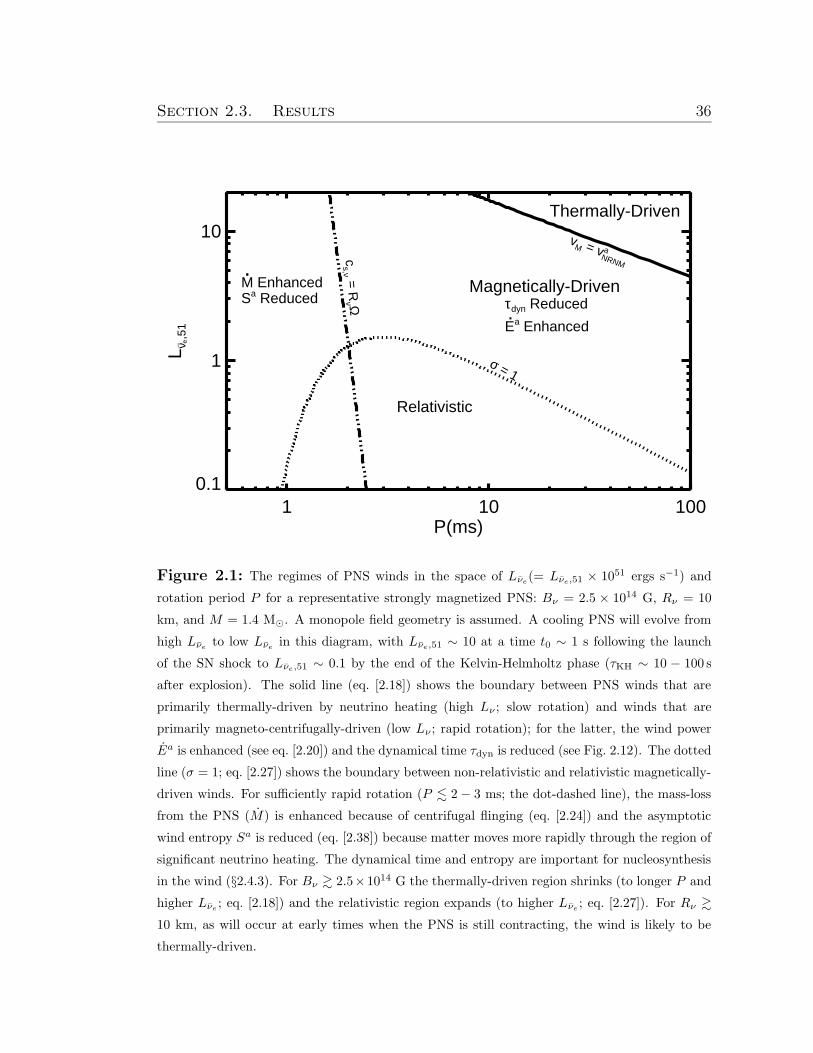
Section 2.3. Results 36
1 10 100P(ms)
0.1
1
10
L ν ,5
1
Thermally-Driven
Magnetically-Drivenτdyn Reduced
Ea Enhanced.
Relativistic
M Enhanced.Sa Reduced
σ = 1
|
e
cs,ν =
Rν Ω
vM = v
NRNM a
Figure 2.1: The regimes of PNS winds in the space of Lνe(= Lνe,51 × 1051 ergs s−1) and
rotation period P for a representative strongly magnetized PNS: Bν = 2.5 × 10¹⁴ G, Rν = 10
km, and M = 1.4 M¯. A monopole field geometry is assumed. A cooling PNS will evolve from
high Lνeto low Lνe
in this diagram, with Lνe,51 ∼ 10 at a time t0 ∼ 1 s following the launch
of the SN shock to Lνe,51 ∼ 0.1 by the end of the Kelvin-Helmholtz phase (τKH ∼ 10 − 100 s
after explosion). The solid line (eq. [2.18]) shows the boundary between PNS winds that are
primarily thermally-driven by neutrino heating (high Lν ; slow rotation) and winds that are
primarily magneto-centrifugally-driven (low Lν ; rapid rotation); for the latter, the wind power
Ea is enhanced (see eq. [2.20]) and the dynamical time τdyn is reduced (see Fig. 2.12). The dotted
line (σ = 1; eq. [2.27]) shows the boundary between non-relativistic and relativistic magnetically-
driven winds. For sufficiently rapid rotation (P . 2− 3 ms; the dot-dashed line), the mass-loss
from the PNS (M) is enhanced because of centrifugal flinging (eq. [2.24]) and the asymptotic
wind entropy Sa is reduced (eq. [2.38]) because matter moves more rapidly through the region of
significant neutrino heating. The dynamical time and entropy are important for nucleosynthesis
in the wind (§2.4.3). For Bν & 2.5×10¹⁴ G the thermally-driven region shrinks (to longer P and
higher Lνe; eq. [2.18]) and the relativistic region expands (to higher Lνe
; eq. [2.27]). For Rν &
10 km, as will occur at early times when the PNS is still contracting, the wind is likely to be
thermally-driven.
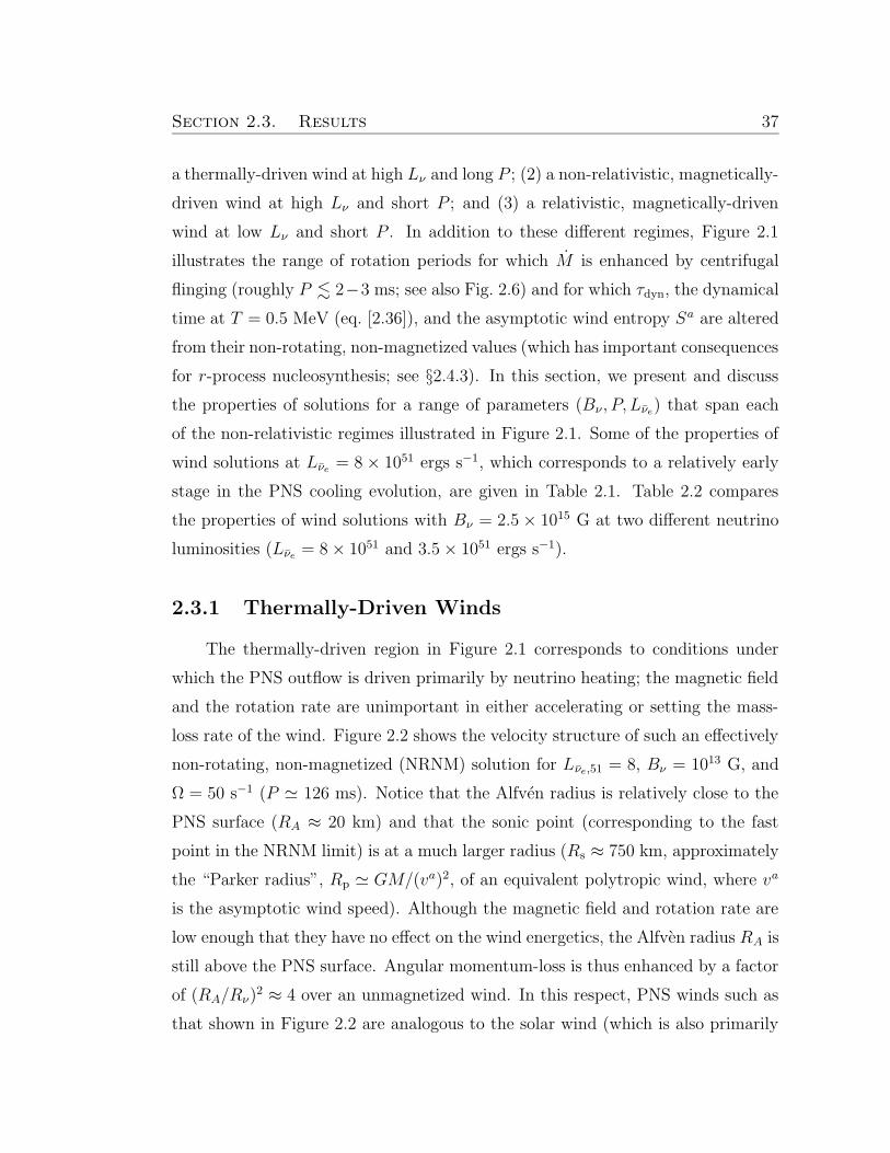
Section 2.3. Results 37
a thermally-driven wind at high Lν and long P ; (2) a non-relativistic, magnetically-
driven wind at high Lν and short P ; and (3) a relativistic, magnetically-driven
wind at low Lν and short P . In addition to these different regimes, Figure 2.1
illustrates the range of rotation periods for which M is enhanced by centrifugal
flinging (roughly P . 2−3 ms; see also Fig. 2.6) and for which τdyn, the dynamical
time at T = 0.5 MeV (eq. [2.36]), and the asymptotic wind entropy Sa are altered
from their non-rotating, non-magnetized values (which has important consequences
for r-process nucleosynthesis; see §2.4.3). In this section, we present and discuss
the properties of solutions for a range of parameters (Bν , P, Lνe) that span each
of the non-relativistic regimes illustrated in Figure 2.1. Some of the properties of
wind solutions at Lνe = 8× 1051 ergs s−1, which corresponds to a relatively early
stage in the PNS cooling evolution, are given in Table 2.1. Table 2.2 compares
the properties of wind solutions with Bν = 2.5× 10¹⁵ G at two different neutrino
luminosities (Lνe = 8× 1051 and 3.5× 1051 ergs s−1).
2.3.1 Thermally-Driven Winds
The thermally-driven region in Figure 2.1 corresponds to conditions under
which the PNS outflow is driven primarily by neutrino heating; the magnetic field
and the rotation rate are unimportant in either accelerating or setting the mass-
loss rate of the wind. Figure 2.2 shows the velocity structure of such an effectively
non-rotating, non-magnetized (NRNM) solution for Lνe,51 = 8, Bν = 1013 G, and
Ω = 50 s−1 (P ' 126 ms). Notice that the Alfven radius is relatively close to the
PNS surface (RA ≈ 20 km) and that the sonic point (corresponding to the fast
point in the NRNM limit) is at a much larger radius (Rs ≈ 750 km, approximately
the “Parker radius”, Rp ' GM/(va)2, of an equivalent polytropic wind, where va
is the asymptotic wind speed). Although the magnetic field and rotation rate are
low enough that they have no effect on the wind energetics, the Alfven radius RA is
still above the PNS surface. Angular momentum-loss is thus enhanced by a factor
of (RA/Rν)2 ≈ 4 over an unmagnetized wind. In this respect, PNS winds such as
that shown in Figure 2.2 are analogous to the solar wind (which is also primarily
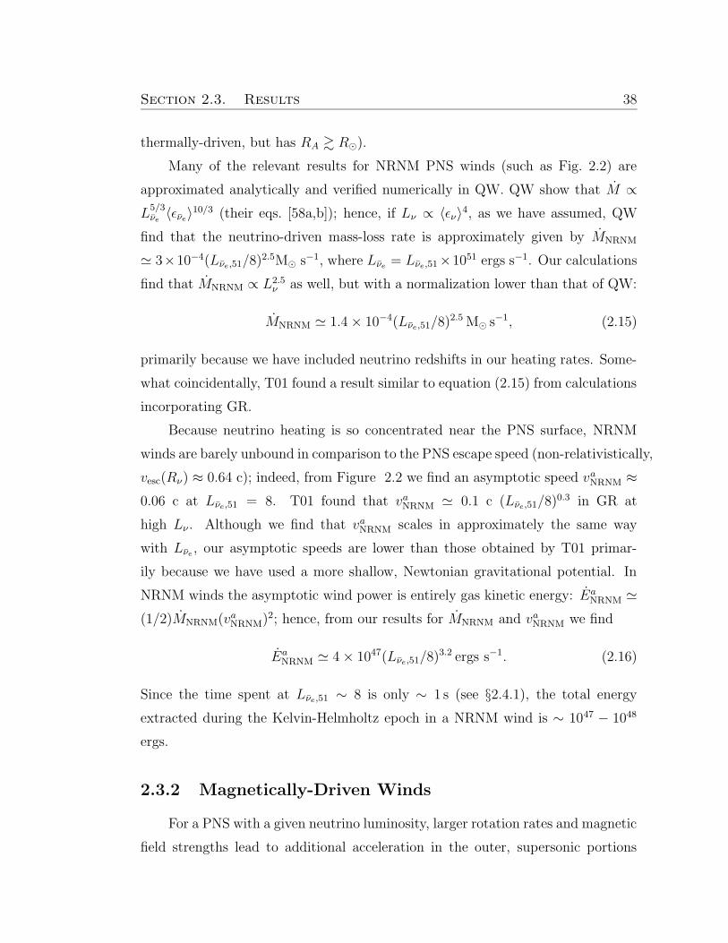
Section 2.3. Results 38
thermally-driven, but has RA & R¯).
Many of the relevant results for NRNM PNS winds (such as Fig. 2.2) are
approximated analytically and verified numerically in QW. QW show that M ∝
L5/3νe 〈ενe〉
10/3 (their eqs. [58a,b]); hence, if Lν ∝ 〈εν〉4, as we have assumed, QW
find that the neutrino-driven mass-loss rate is approximately given by MNRNM
' 3×10⁻⁴(Lνe,51/8)2.5M¯ s−1, where Lνe = Lνe,51×1051 ergs s−1. Our calculations
find that MNRNM ∝ L2.5ν as well, but with a normalization lower than that of QW:
MNRNM ' 1.4× 10⁻⁴(Lνe,51/8)2.5 M¯ s
−1, (2.15)
primarily because we have included neutrino redshifts in our heating rates. Some-
what coincidentally, T01 found a result similar to equation (2.15) from calculations
incorporating GR.
Because neutrino heating is so concentrated near the PNS surface, NRNM
winds are barely unbound in comparison to the PNS escape speed (non-relativistically,
vesc(Rν) ≈ 0.64 c); indeed, from Figure 2.2 we find an asymptotic speed vaNRNM ≈
0.06 c at Lνe,51 = 8. T01 found that vaNRNM ' 0.1 c (Lνe,51/8)0.3 in GR at
high Lν . Although we find that vaNRNM scales in approximately the same way
with Lνe , our asymptotic speeds are lower than those obtained by T01 primar-
ily because we have used a more shallow, Newtonian gravitational potential. In
NRNM winds the asymptotic wind power is entirely gas kinetic energy: EaNRNM '
(1/2)MNRNM(vaNRNM)
2; hence, from our results for MNRNM and vaNRNM we find
EaNRNM ' 4× 1047(Lνe,51/8)
3.2 ergs s−1. (2.16)
Since the time spent at Lνe,51 ∼ 8 is only ∼ 1 s (see §2.4.1), the total energy
extracted during the Kelvin-Helmholtz epoch in a NRNM wind is ∼ 1047 − 1048
ergs.
2.3.2 Magnetically-Driven Winds
For a PNS with a given neutrino luminosity, larger rotation rates and magnetic
field strengths lead to additional acceleration in the outer, supersonic portions
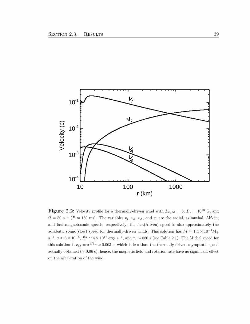
Section 2.3. Results 39
10 100 1000r (km)
10-4
10-3
10-2
10-1
Vel
ocity
(c)
vf
vr
vφ
vA
Figure 2.2: Velocity profile for a thermally-driven wind with Lνe,51 = 8, Bν = 1013 G, and
Ω = 50 s−1 (P ≈ 130 ms). The variables vr, vφ, vA, and vf are the radial, azimuthal, Alfven,
and fast magnetosonic speeds, respectively; the fast(Alfven) speed is also approximately the
adiabatic sound(slow) speed for thermally-driven winds. This solution has M ≈ 1.4 × 10⁻⁴M¯
s−1, σ ≈ 3× 10⁻⁸, Ea ' 4× 1047 ergs s−1, and τJ ∼ 880 s (see Table 2.1). The Michel speed for
this solution is vM = σ1/3c ' 0.003 c, which is less than the thermally-driven asymptotic speed
actually obtained (≈ 0.06 c); hence, the magnetic field and rotation rate have no significant effect
on the acceleration of the wind.
Section 2.3. Results 40
10 100 1000r (km)
0.0
0.1
0.2
0.3
0.4
0.5
0.6
0.7
Vel
ocity
(c)
vf
vr
vφ
vA
vs
Figure 2.3: Velocity profile for a magneto-centrifugally-driven wind with Lνe,51 = 8, Bν =
1015 G, and Ω = 5000 s−1 (P ' 1.26 ms); the variables vr, vφ, vA, vf , and vs are the radial,
azimuthal, Alfven, fast, and slow magnetosonic speeds, respectively. This solution has M '
3.0 × 10⁻³M¯ s−1, σ ' 0.16, τJ ' 9 s, and Ea ' 2.3 × 1051 ergs s−1. Comparison plots of
vr and vφ (dashed lines) are for a γ = 1.15 polytropic wind with similar M , Ω, Bν , and inner
temperature. Notice that the radius of the slow point (approximately the sonic point; where
vr = vs) is very close to the value expected in the magneto-centrifugal limit: Rs,cf ≈ 19.6 km
(eq. [2.19]).
Section 2.3. Results 41
of the wind. If the rotation rate and magnetic field are high enough, they will
dominate the wind acceleration at large radii. This is the “Fast Magnetic Rotator”
(FMR) limit, using the stellar-wind terminology of Belcher & MacGregor (1976);
see also Lamers & Cassinelli (1999). An approximate criteria for this limit is that
the magnetically-driven asymptotic speed, given roughly by the Michel speed vM ≡
(B2νR
4νΩ
2/M)1/3 = σ1/3c (Michel 1969), exceeds the asymptotic speed obtained if
the wind were entirely thermally-driven by neutrino heating (vaNRNM). Using our
result for vaNRNM, the wind will be in the FMR limit for magnetizations
σ & 2× 10⁻⁴(Lνe,51/8)0.9 ≡ σFMR. (2.17)
Using equation (2.15) to relate Lνe and M , our calculations imply that the PNS
wind is magnetically-driven below the critical rotation period
PFMR ' 15 (Lνe,51/8)−1.7B14ms, (2.18)
where Bν = Bn × 10n G. The P = PFMR boundary in Figure 2.1 is marked by
a solid line. The magnetically-driven regime encompasses a large range of PNS
parameter space and hence generically describes most of a strongly magnetized
PNS’s evolution. In contrast, the wind from a relatively weakly magnetized PNS
will only be dominated by magneto-centrifugal forces late in the cooling epoch.
The conditions necessary for the magnetically-driven phase to dominate the total
energy and mass-loss during the Kelvin-Helmholtz phase will be discussed further
in §2.4.1.
Figure 2.3 shows the velocity structure of a magnetically-driven wind from
a PNS with Lνe,51 = 8, Bν = 1015 G and Ω = 5000 s−1 (P ' 1.3 ms). As the
profile of vφ in Figure 2.3 indicates, the wind corotates to ≈ 25 km, which is far
inside RA ≈ 46 km because the magnetic field carries a significant fraction of the
angular momentum. In addition, because the wind is magnetically-driven, the
wind speed at large radii is almost an order of magnitude larger than in a NRNM
wind: vr = 0.54 c ≈ vM obtains at the outer grid point. The sonic point of the wind
(corresponding to the slow point in the FMR limit) is now inside RA, less than one
stellar radius off the surface; this is expected because analytic considerations show
Section 2.3. Results 42
that with increasing Ω, the location of the sonic radius Rs decreases from a value
of order the Parker radius to a value independent of the local thermodynamics (see
Lamers & Cassinelli 1999)2:
Rs,cf ≡(
GM/Ω2)1/3' 17P 2/3
ms km. (2.19)
For comparison with our solution, Figure 2.3 shows the velocity structure of an
adiabatic wind (γ = 1.15) with approximately the same M , Ω, Bν , and surface
temperature as our neutrino-heated wind. The adiabatic solution agrees well with
the neutrino-heated solution because, although M is primarily set by Lν , once
M is specified the velocity structure of the magnetically-driven wind becomes
relatively independent of the details of the neutrino microphysics. This agreement
implies that we can accurately map our 1D neutrino-heated calculations onto multi-
dimensional polytropic calculations that employ similar boundary conditions and
a similar effective adiabatic index (see §2.4.1).
For FMR winds, the Michel speed obtains at large radii and the asymptotic
wind power is therefore enhanced relative to equation (2.16):
EaFMR = MBa ' (3/2)Mv2M '
1050B4/314 M
1/3−3 P
−4/3ms ergs s−1, (2.20)
where M = M−3 × 10⁻³ M¯s−1 and Ba = Ea/M = (v3M/v
a) + (va)2/2 ' (3/2)v2M
is the Bernoulli integral at large radii in the FMR limit, and is composed of 2/3
magnetic and 1/3 kinetic energy.
To calculate the angular momentum lost by the PNS, we note that for any
super-Alfvenic outflow, equation (2.7), equation (2.8), and conservation of mag-
netic flux require that the conserved specific angular momentum obey L = ΩR2A,
where RA is defined by the position where the radial outflow speed matches the
radial Alfven speed: vr(RA) = Br(RA)/√
4πρ(RA) ≡ vA. We estimate the loca-
tion of the Alfven point in terms of η = ΩJ/Ea = Ω2R2A/B
a defined in equation
(2.12):
R2AΩ
2 ' (3/2)ηv2M , (2.21)2The subscript “cf”, here and below, stands for “centrifugal” and relates to the limit described
by equation (2.25).
Section 2.3. Results 43
so that3
RA|FMR ' 11 η1/2B2/314 M
−1/3−3 P 1/3
ms km. (2.22)
Figure 2.4 shows η for our wind solutions with Lνe,51 = 8 for several surface
magnetic field strengths (see also Table 2.1). Recall that 1/η represents the fraction
of the extracted rotational energy from the PNS available to energize the surround-
ing environment. In the limit that vM & vesc, we find that η ≈ 1 and almost all of
the rotational energy lost by the PNS emerges as asymptotic wind power; this limit
is normally assumed when considering magnetized stellar spin-down. However, as
the low Bν solutions in Figure 2.4 illustrate, winds with short rotation periods and
vaNRNM < vM < vesc can be magnetically-driven and yet have η À 1. The primary
reason for this is that at high Ω the neutrino heating rate per unit mass is sig-
nificantly reduced below its NRNM value because centrifugally-accelerated matter
spends less time in the region where neutrino heating is important. Because the
wind absorbs less of the neutrino energy, the magnetic field becomes more impor-
tant for unbinding the matter from the PNS. Consequently, only a fraction of the
rotational energy extracted at the PNS surface reaches large radii.
In the limit of thermally-driven solutions with very low Bν (even lower than
in Fig. 2.2, such that the Alfven radius is interior to the stellar surface), Rν
is the lever arm for angular momentum-loss; thus L = ΩR2ν and hence η =
Ω2R2νMNRNM/E
aNRNM ≈ 24(Lνe,51/8)
−0.6P−2ms (using eqs. [2.15] and [2.16]). For
P À 1 ms thermally-driven winds have η ¿ 1, which explains why η decreases
rapidly for solutions with large P in Figure 2.4. Physically, this is because for slow
rotation rates the rotational power lost by the PNS is insignificant in comparison
to the thermal energy supplied by neutrino heating.
The rate at which angular momentum is extracted from the PNS is J = IΩ =
ΩR2AM , where J = IΩ is the angular momentum of the PNS and I ' (2/5)MR2
ν is
the PNS moment of inertia. Hence, given the Alfven radius from equation (2.22),
the spin-down time of the PNS (τJ ≡ Ω/Ω) in the non-relativistic, magnetically-
3TCQ took ΩRA = vr(RA) = vM and assumed η = 1. We find that in some circumstancesthe η = 1 assumption is not applicable, even in the FMR limit (see Fig. 2.4).
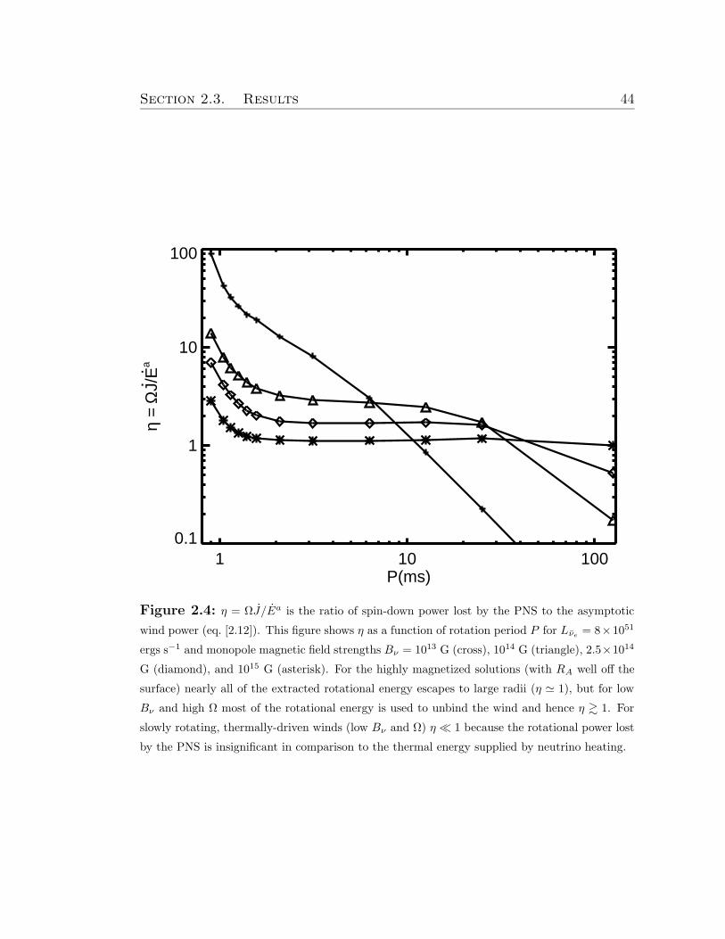
Section 2.3. Results 44
1 10 100P(ms)
0.1
1
10
100
η =
ΩJ/
Ea.
.
Figure 2.4: η = ΩJ/Ea is the ratio of spin-down power lost by the PNS to the asymptotic
wind power (eq. [2.12]). This figure shows η as a function of rotation period P for Lνe= 8×1051
ergs s−1 and monopole magnetic field strengths Bν = 1013 G (cross), 1014 G (triangle), 2.5×10¹⁴
G (diamond), and 1015 G (asterisk). For the highly magnetized solutions (with RA well off the
surface) nearly all of the extracted rotational energy escapes to large radii (η ' 1), but for low
Bν and high Ω most of the rotational energy is used to unbind the wind and hence η & 1. For
slowly rotating, thermally-driven winds (low Bν and Ω) η ¿ 1 because the rotational power lost
by the PNS is insignificant in comparison to the thermal energy supplied by neutrino heating.
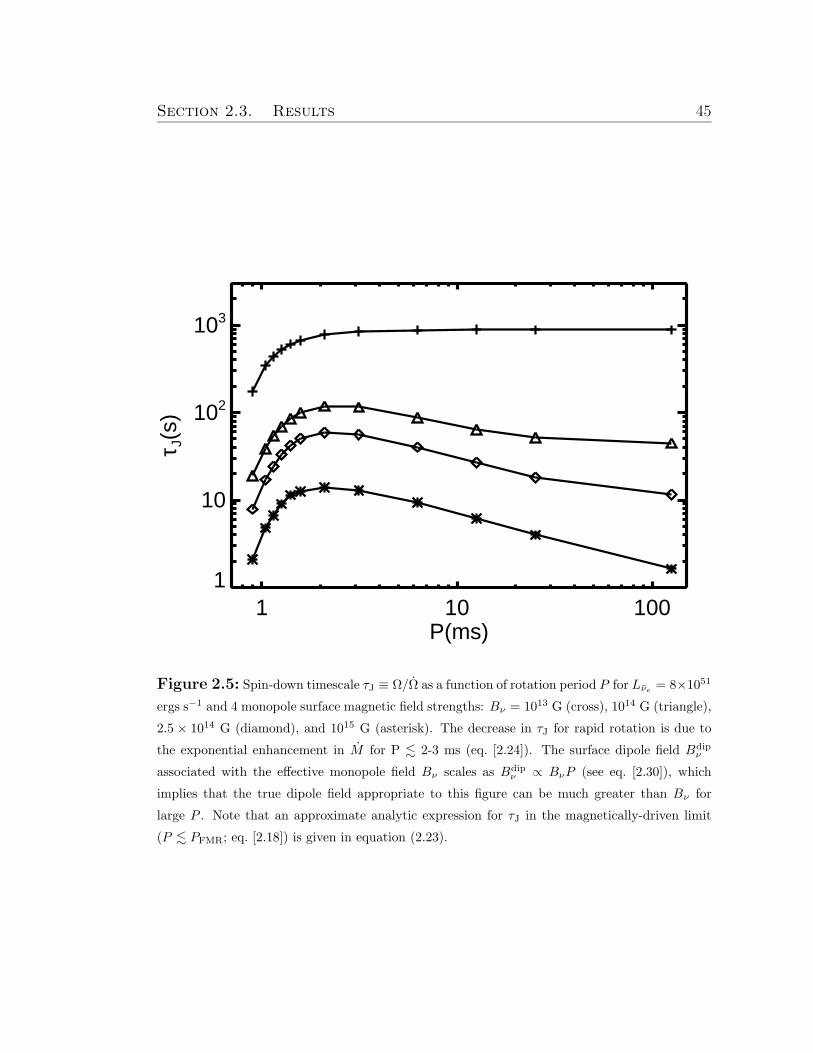
Section 2.3. Results 45
1 10 100P(ms)
1
10
102
103
τ J(s
)
Figure 2.5: Spin-down timescale τJ ≡ Ω/Ω as a function of rotation period P for Lνe= 8×1051
ergs s−1 and 4 monopole surface magnetic field strengths: Bν = 1013 G (cross), 1014 G (triangle),
2.5 × 10¹⁴ G (diamond), and 1015 G (asterisk). The decrease in τJ for rapid rotation is due to
the exponential enhancement in M for P . 2-3 ms (eq. [2.24]). The surface dipole field Bdipν
associated with the effective monopole field Bν scales as Bdipν ∝ BνP (see eq. [2.30]), which
implies that the true dipole field appropriate to this figure can be much greater than Bν for
large P . Note that an approximate analytic expression for τJ in the magnetically-driven limit
(P . PFMR; eq. [2.18]) is given in equation (2.23).
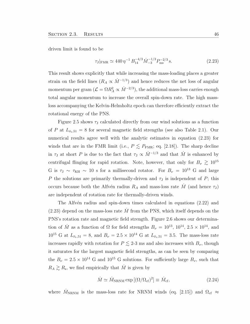
Section 2.3. Results 46
driven limit is found to be
τJ|FMR ' 440 η−1B−4/314 M
−1/3−3 P−2/3ms s. (2.23)
This result shows explicitly that while increasing the mass-loading places a greater
strain on the field lines (RA ∝ M−1/3) and hence reduces the net loss of angular
momentum per gram (L = ΩR2A ∝ M−2/3), the additional mass-loss carries enough
total angular momentum to increase the overall spin-down rate. The high mass-
loss accompanying the Kelvin-Helmholtz epoch can therefore efficiently extract the
rotational energy of the PNS.
Figure 2.5 shows τJ calculated directly from our wind solutions as a function
of P at Lνe,51 = 8 for several magnetic field strengths (see also Table 2.1). Our
numerical results agree well with the analytic estimates in equation (2.23) for
winds that are in the FMR limit (i.e., P . PFMR; eq. [2.18]). The sharp decline
in τJ at short P is due to the fact that τJ ∝ M−1/3 and that M is enhanced by
centrifugal flinging for rapid rotation. Note, however, that only for Bν & 1015
G is τJ ∼ τKH ∼ 10 s for a millisecond rotator. For Bν = 1013 G and large
P the solutions are primarily thermally-driven and τJ is independent of P ; this
occurs because both the Alfven radius RA and mass-loss rate M (and hence τJ)
are independent of rotation rate for thermally-driven winds.
The Alfven radius and spin-down times calculated in equations (2.22) and
(2.23) depend on the mass-loss rate M from the PNS, which itself depends on the
PNS’s rotation rate and magnetic field strength. Figure 2.6 shows our determina-
tion of M as a function of Ω for field strengths Bν = 1013, 1014, 2.5 × 10¹⁴, and
1015 G at Lνe,51 = 8, and Bν = 2.5 × 10¹⁴ G at Lνe,51 = 3.5. The mass-loss rate
increases rapidly with rotation for P . 2-3 ms and also increases with Bν , though
it saturates for the largest magnetic field strengths, as can be seen by comparing
the Bν = 2.5 × 10¹⁴ G and 1015 G solutions. For sufficiently large Bν , such that
RA & Rs, we find empirically that M is given by
M ' MNRNM exp [(Ω/Ωcf)2] ≡ Mcf , (2.24)
where MNRNM is the mass-loss rate for NRNM winds (eq. [2.15]) and Ωcf ≈
Section 2.3. Results 47
2000 4000 6000Ω(s-1)
10-5
10-4
10-3
10-2
10-1
M (
M /
s)
........................................................................................................................................................................................................................................................................................................................................................................................................................................................................................................................................................................................................................................................................................................................................................................................................................................................................................................................................................................................................................................................................................................................................................................................................................................................................................................................................................................................................................................................................................................................................................................................................................................................................................................................................................................................................................................................................................................................................................................................................................................................................................................................................................................................................................................................................................................................................................................................................................................................................................
.
Figure 2.6: mass-loss rate M as a function of the rotation rate Ω at Lνe= 8× 1051 ergs s−1
for Bν = 1013 G (cross), Bν = 1014 G (triangle), 2.5× 10¹⁴ G (diamond), and 1015 G (asterisk);
also shown is M(Ω) for Lνe= 3.5 × 1051 ergs s−1 and Bν = 2.5 × 10¹⁴ G (dotted, diamond).
M increases with increasing Ω and Bν because centrifugal support expands the hydrostatic
atmosphere (see Fig. 2.7). For sufficiently large Bν (& Bcf ; eq. [2.26]), however, M(Ω) no longer
increases with increasing Bν because the wind corotates past the sonic point. An approximate
fit to the numerical results in this limit is given by equation (2.24).
Section 2.3. Results 48
2700(Lνe,51/8)0.08 s−1.
The enhanced mass-loss shown in Figure 2.6 is due to the effect of strong
magnetic fields and rapid rotation on the subsonic, hydrostatic structure of PNS
winds. Figures 2.7 and 2.8 show the density and temperature profiles, respectively,
for winds with Bν = 1015 G and Lνe,51 = 8 at several rotation rates. For the most
rapidly rotating solution (solid line), Figure 2.7 shows that centrifugal support is
sufficient to expand the scale height of the hydrostatic atmosphere at small radii,
resulting in the much higher mass-loss rates seen in Figure 2.6. Analytically, we
expect the centrifugal support to be important when RνΩ & cs,ν , where cs,ν is
the sound speed at the PNS neutrinosphere. We find that the inner sound speed
depends only weakly on the neutrino luminosity: cs,ν ≈ 0.12(Lνe,51/8)0.08 c, and
thus that mass-loss is enhanced for
Ω & 3600(Lνe,51/8)0.08 s−1. (2.25)
This region is denoted “M Enhanced” in Figure 2.1. Equation (2.25) is in good
agreement with our numerically determined value of Ωcf defined in equation (2.24).
The enhancement of M implied by equations (2.24) and (2.25) does not ex-
plicitly depend on the magnetic field strength. However, centrifugal support of the
PNS atmosphere only occurs if the field can sustain corotation out to the sonic
radius Rs; otherwise rotation has much less of an effect on the mass-loss rate (see
the solutions with low Bν in Fig. 2.6). The requirement of corotation out to Rs
can be written as RA > Rs,cf (eq. [2.19]), which in turn implies Bν > Bcf , where
Bcf ' 2× 10¹⁴ η−3/4M1/2−3 P
1/2ms G. (2.26)
For Bν & Bcf , the mass-loss from the PNS no longer increases with increasing Bν
(see Fig. 2.6) because the wind already co-rotates out to the sonic radius where
M is set. In deriving Bcf in equation (2.26), we have used equation (2.22) for
RA because, under most conditions, a wind that is centrifugally-supported will
automatically be in the FMR limit, although the converse is not necessarily true.
We note that even relatively weakly-magnetized PNS’s that are rapidly rotating
will experience some degree of enhanced mass-loss. For instance, for Ω = 7000 s−1,
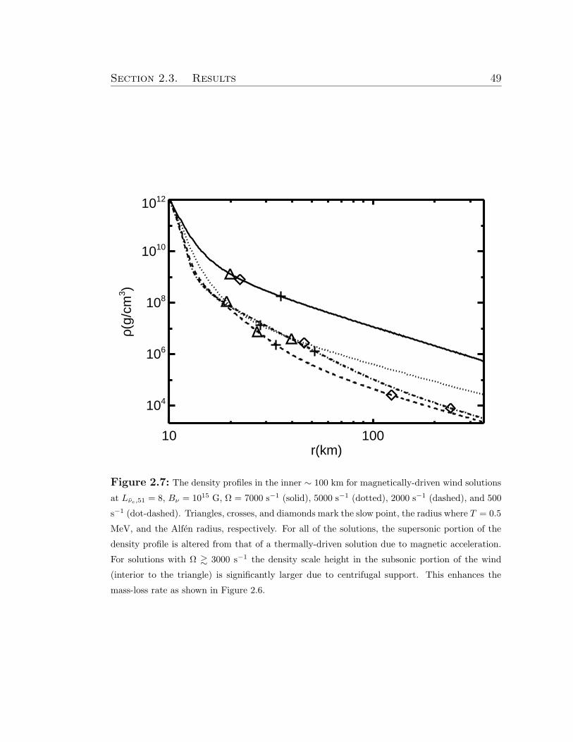
Section 2.3. Results 49
10 100r(km)
104
106
108
1010
1012
ρ(g/
cm3 )
Figure 2.7: The density profiles in the inner ∼ 100 km for magnetically-driven wind solutions
at Lνe,51 = 8, Bν = 1015 G, Ω = 7000 s−1 (solid), 5000 s−1 (dotted), 2000 s−1 (dashed), and 500
s−1 (dot-dashed). Triangles, crosses, and diamonds mark the slow point, the radius where T = 0.5
MeV, and the Alfen radius, respectively. For all of the solutions, the supersonic portion of the
density profile is altered from that of a thermally-driven solution due to magnetic acceleration.
For solutions with Ω & 3000 s−1 the density scale height in the subsonic portion of the wind
(interior to the triangle) is significantly larger due to centrifugal support. This enhances the
mass-loss rate as shown in Figure 2.6.
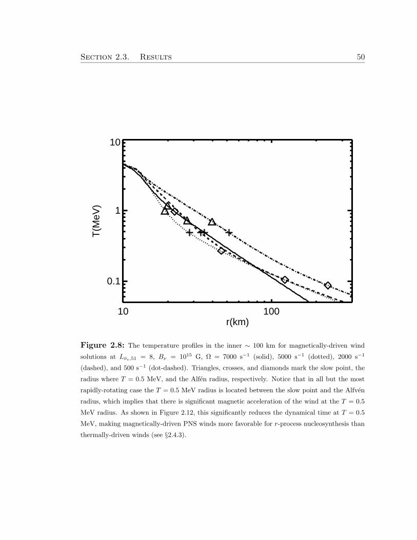
Section 2.3. Results 50
10 100r(km)
0.1
1
10
T(M
eV)
Figure 2.8: The temperature profiles in the inner ∼ 100 km for magnetically-driven wind
solutions at Lνe,51 = 8, Bν = 1015 G, Ω = 7000 s−1 (solid), 5000 s−1 (dotted), 2000 s−1
(dashed), and 500 s−1 (dot-dashed). Triangles, crosses, and diamonds mark the slow point, the
radius where T = 0.5 MeV, and the Alfen radius, respectively. Notice that in all but the most
rapidly-rotating case the T = 0.5 MeV radius is located between the slow point and the Alfven
radius, which implies that there is significant magnetic acceleration of the wind at the T = 0.5
MeV radius. As shown in Figure 2.12, this significantly reduces the dynamical time at T = 0.5
MeV, making magnetically-driven PNS winds more favorable for r-process nucleosynthesis than
thermally-driven winds (see §2.4.3).
Section 2.4. Applications and Discussion 51
even the lowest field strength solution in Figure 2.6 (Bν = 1013 G) has a mass-loss
rate almost an order of magnitude larger than its NRNM value.
The non-relativistic calculations we have presented here are only applicable
for magnetizations σ < 1; this is equivalent to requiring RA < RL ≡ c/Ω, the
radius of the light cylinder. For σ > 1 the PNS wind becomes relativistic and
its spin-down properties will change (see §2.4.1 for a discussion). Using equation
(2.24) for M (i.e., assuming Bν > Bcf), the magnetization is given by
σ ' 0.05B214P
−2ms (Lνe,51/8)
−2.5 exp[−5.4P−2ms (Lνe,51/8)−0.16]. (2.27)
The σ = 1 boundary is denoted by a dotted line in Figure 2.1. PNSs with σ > 1
and Lνe,51 & 0.1 will experience a relativistic phase accompanied by significant
mass-loss; this mass-loss keeps the wind mildly relativistic, in contrast to the
much higher σ spin-down that will commence following τKH (Lνe,51 ¿ 0.1).
2.4 Applications and Discussion
2.4.1 Magnetized PNS Evolution
With our numerical results in hand that sample a wide range of PNS wind
conditions, we can begin to address the time evolution of a cooling, magnetized
PNS. In the early stages following the launch of SN shock the PNS is likely hot and
inflated, with a radius exceeding the value of Rν = 10 km that we have assumed
in all of the calculations presented in this paper. This early phase is likely to be
thermally-driven for all but the most highly-magnetized proto-magnetars, and, if
a dynamo is at work, the large-scale field itself may still be amplifying during this
phase (Thompson & Duncan 1993). Using the collapse calculations of Bruenn, De
Nisco, & Mezzacappa (2001) (from a 15 M¯ progenitor of Woosley & Weaver 1995)
T01 fit an approximate functional form to the PNS radial contraction: Rν ∝ t−1/3
such that Rν(1 s) ' 15 km and Rν(2 s) ' 12 km. The recent SN simulations
of Buras et al. (2003, 2006) with Boltzmann neutrino transport find a similar
neutrinosphere radius at t ∼ 1 s after bounce.
Section 2.4. Applications and Discussion 52
We do not attempt to address the uncertainties in early-time PNS cooling
calculations, especially in the presence of large fields and rapid rotation. Rather,
we assume that the PNS has cooled to its final radius and completely established
its global field by a time t0 ∼ 1 s following core-collapse; we can then use the
calculations presented in this paper to investigate the subsequent evolution of the
PNS. Following t0 we assume a simplified PNS cooling evolution (similar to that
used in TCQ, motivated by Figure 14 of Pons et al. 1999):
Lνe,51(t) = L0
(
t
τKH
)−δ
: t0 < t < τKH
Lνe,51(t) = L0 exp[−(t− τKH)/τKH] : t > τKH, (2.28)
where, for definitiveness in what follows, we take L0 = 0.2, t0 = 1 s, τKH = 40
s, and δ = 1. This cooling evolution is approximate because magnetar-strength
fields and rapid rotation could alter τKH or the form of the cooling profile (e.g.,
δ) by affecting the neutrino opacity or the dynamics of the contraction itself (e.g.,
Villain et al. 2004; Dessart et al. 2006). For instance, in 1D collapse calculations
with rotation, Thompson, Quataert, & Burrows (2005) found that for P ∼ 1 ms,
the total neutrino luminosity at t ' 0.6 s after bounce is ∼ 50% smaller than in a
non-rotating PNS.
The dominant uncertainty in applying our results to magnetized PNS evo-
lution is that we have assumed a monopole field geometry. To relate our results
to more realistic dipole simulations, we use the recent axisymmetric, relativistic
MHD simulations of B06, who simulate neutron star spin-down for σ ≈ 0.3 − 20.
B06 show that the energy and angular momentum-loss rates from aligned dipole
spin-down can be described accurately by monopole formulae provided they are
normalized to just the open magnetic flux; for instance, we can accurately apply
our results for τJ (eq. [2.23]) with a suitable renormalization of Bν .
To apply the results of B06 we need to estimate the open magnetic flux in
PNS winds. In force-free spin-down calculations motivated by pulsars it is generally
assumed that the radius of the last closed magnetic field line (the “Y point” RY )
is coincident with the light cylinder (Contopoulos et al. 1999; Gruzinov 2005)
so that the ratio between the fraction of open magnetic flux in the dipole and
Section 2.4. Applications and Discussion 53
monopole cases is Rν/RY = Rν/RL. This assumption is supported by force-
free simulations (Spitkovsky 2006; McKinney 2006), which show that when mass-
loading is completely negligible (σ → ∞), RY ' RL. However, B06 show that
rapidly rotating, mildly mass-loaded MHD winds have a larger percentage of open
magnetic flux than vacuum or force-free spin-down would imply (i.e., RY < RL).
From Table 4 of B06 we fit the approximate power law
RY /RL ' 0.31σ0.15 (2.29)
for the range σ ∈ [0.298, 17.5] and for a fixed rotation period of order one mil-
lisecond. Although there are uncertainties in quantitatively extrapolating B06’s
results, reaching the pure force-free limit with RY ' RL appears to require σ À 1.
We therefore conclude that magnetized, rapidly rotating PNS winds (with σ ∈
10−3, 103 for t < τKH under most circumstances) will typically possess excess
open magnetic flux.
Because the results of B06 for RY /RL cover only a relatively narrow portion
of PNS parameter-space we must proceed with caution in generalizing their results
to our calculations; on the other hand, their basic conclusion shows a weak depen-
dence on σ and Ω, and has a solid theoretical explanation (Mestel & Spruit 1987).
Hence, we have attempted to apply the results of B06 to gain insight into the
multi-dimensional generalization of our calculations, but we check at every step
that our calculations are not overly sensitive to extrapolations of B06’s results.
Combining equation (2.29) with the empirical formula B06 provide (their eq. [25])
relating the effective monopole surface field Bmonν to the true equatorial dipole field
Bdipν we find
Bmonν ' 0.6Bdip
ν
Rν
RL
(
RY
RL
)−1
' 0.4Bdipν P−1ms σ
−0.15, (2.30)
which remains approximately valid for a substantial range in σ, provided we enforce
RY = RL for σ & 103 and keep RY > Rν .
Using equation (2.30) we substitute Bmonν for Bν in the results of §2.3 and
integrate from t0 to τKH using our fiducial cooling evolution (eq. [2.28]) to obtain
the total energy and mass-loss during the Kelvin-Helmholtz epoch (Eatot and ∆Mtot,
Section 2.4. Applications and Discussion 54
respectively) as a function of the fixed dipole surface field Bdipν and for initial
rotation periods P0 ∈ 1, 10 ms. Although a neutron star will eventually impart
any remaining rotational energy after τKH to its surroundings through an ultra-
relativistic, pulsar-like outflow, we concentrate on the wind evolution prior to the
end of the Kelvin-Helmholtz phase because our calculations are primarily suited to
studying mass-loaded spin-down and because we are interested in energy that can
be extracted sufficiently early to affect the rapidly outward-propagating SN shock.
In performing our calculations when the wind is relativistic (σ > 1), we continue
using equation (2.24) for M and employ the relativistic spin-down formula given
by B06 (their eq. [26]):
EaREL ' 1.5× 1047(Bdip
14 )2P−4ms
(
RY
RL
)−2
ergs s−1, (2.31)
evaluated for RY /RL given by equation (2.29).
Although it is possible that equation (2.29) may not be accurate far outside
the parameter regime B06 considered, we found that re-running the calculations
at fixed RY/RL = 1/3 changed Eatot by, at most, a factor of a few. A similar
uncertainty in our calculations is that we have used our equatorial M over all 4π
steradian; thus, we have probably overestimated ∆Mtot by a factor of ∼ 2 due to
the effects of closed magnetic flux and because centrifugal flinging concentrates M
at low latitudes. Although a direct comparison of the mass-loss rate between our
solutions and the dipole simulations of B06 is difficult, we find that the dependence
of M on Ω is similar between our solutions when the surface temperature in B06’s
simulations is scaled to an appropriate neutrino luminosity.
Our estimates for Eatot and ∆Mtot during the Kelvin-Helmholtz phase are
presented in Figures 2.9 and 2.10 for values of Bdipν ranging from 1012 − 1016
G. The single dominant phase contributing the majority of the energy extracted
for a given initial rotation rate P0 is denoted by the line style (thermally-driven
[NRNM] = dotted; non-relativistic, magnetically-driven [FMR] = solid; relativis-
tic, magnetically-driven [REL] = 3 dot-dash). While all PNSs pass through each
wind phase sometime during τKH (see Fig. 2.1), PNSs can still be usefully classi-
fied into 3 types based on which wind phase dominates the total energy-loss during
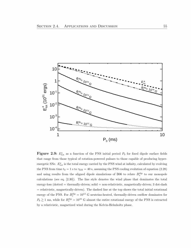
Section 2.4. Applications and Discussion 55
1 10P0 (ms)
10-4
10-3
10-2
10-1
1
10
Eto
t (10
51 e
rgs)
a
Bν = 1012 Gdip
Bν = 10 13 G
dip
Bν = 10 14 G
dip
Bν = 10 15 G
dip
Bν = 10 16 Gdip
Erota
Figure 2.9: Eatot as a function of the PNS initial period P0 for fixed dipole surface fields
that range from those typical of rotation-powered pulsars to those capable of producing hyper-
energetic SNe. Eatot is the total energy carried by the PNS wind at infinity, calculated by evolving
the PNS from time t0 = 1 s to τKH = 40 s, assuming the PNS cooling evolution of equation (2.28)
and using results from the aligned dipole simulations of B06 to relate Bdipν to our monopole
calculations (see eq. [2.30]). The line style denotes the wind phase that dominates the total
energy-loss (dotted = thermally-driven; solid = non-relativistic, magnetically-driven; 3 dot-dash
= relativistic, magnetically-driven). The dashed line at the top shows the total initial rotational
energy of the PNS. For Bdipν = 1012 G neutrino-heated, thermally-driven outflow dominates for
P0 & 1 ms, while for Bdipν = 1016 G almost the entire rotational energy of the PNS is extracted
by a relativistic, magnetized wind during the Kelvin-Helmholtz phase.
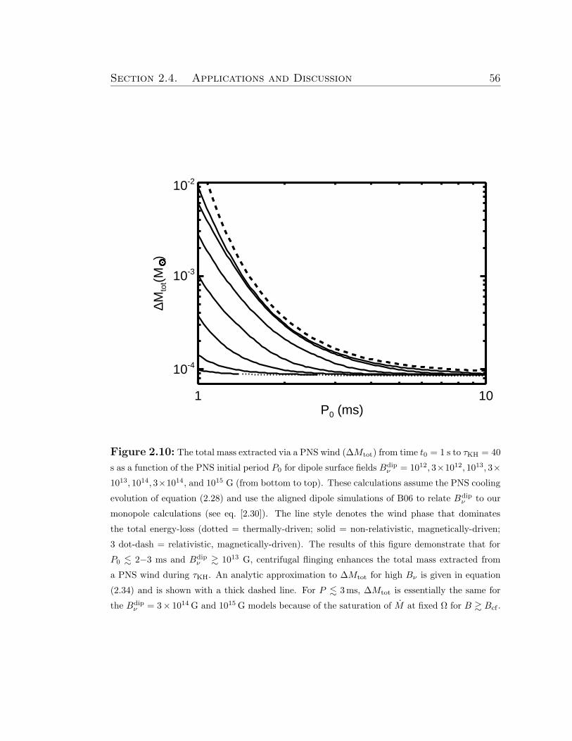
Section 2.4. Applications and Discussion 56
1 10P0 (ms)
10-4
10-3
10-2
∆Mto
t(M )..................................................................................................................................................................
.
.
.
.
.
.
.
.
.
.
.
.
.
.
.
.
.
.
.
.
.
.
.
.
.
.
.
.
.
.
.
.
.
.
.
.
.
.
.
.
.
.
.
.
.
.
.
.
.
.
.
.
.
.
.
.
.
.
.
.
.
.
.
.
.
.
.
.
.
.
.
.
..............................................................................................................................................................................................................................................................................................................................................................................................................................................................................................................................................................................................................................................................................................................................................................................................................................................................................................................................................................................................................................................................................................................................................................................................................................................................................................................................................................................................................................................................................................................................................................................................................................................................................................................................................................................................................................................................................................................................................................................................................................................................................................................................................................................................................................................
Figure 2.10: The total mass extracted via a PNS wind (∆Mtot) from time t0 = 1 s to τKH = 40
s as a function of the PNS initial period P0 for dipole surface fields Bdipν = 1012, 3×10¹², 1013, 3×
1013, 1014, 3×10¹⁴, and 1015 G (from bottom to top). These calculations assume the PNS cooling
evolution of equation (2.28) and use the aligned dipole simulations of B06 to relate Bdipν to our
monopole calculations (see eq. [2.30]). The line style denotes the wind phase that dominates
the total energy-loss (dotted = thermally-driven; solid = non-relativistic, magnetically-driven;
3 dot-dash = relativistic, magnetically-driven). The results of this figure demonstrate that for
P0 . 2−3 ms and Bdipν & 1013 G, centrifugal flinging enhances the total mass extracted from
a PNS wind during τKH. An analytic approximation to ∆Mtot for high Bν is given in equation
(2.34) and is shown with a thick dashed line. For P . 3ms, ∆Mtot is essentially the same for
the Bdipν = 3× 10¹⁴G and 1015G models because of the saturation of M at fixed Ω for B & Bcf .
Section 2.4. Applications and Discussion 57
τKH:
(1) Thermally −DrivenWinds (Bdip14 . 10−2P2
ms) :
For low magnetic field strengths, Figures 2.9 and 2.10 show that the total mass and
energy-loss are effectively at the NRNM values for a large range of initial periods:
∆MNRNMtot ' 10−4(t0/1s)
−1.5M¯, ENRNMtot ' 2 × 1047(t0/1s)
−2.2 ergs. Energy and
mass-loss from this class of PNSs is generally modest and is dominated by early
times. Analysis of the Parkes multibeam survey suggests that half of all pulsars
are born with Bdipν < 3 × 10¹² G (Vranesevic et al. 2004), implying that NRNM
winds dominate the majority of neutron star births, independent of the birth-
period distribution. Spin-down during τKH is negligible for PNSs of this type and
the supernova remnants associated with the production of NRNM PNSs will not
be significantly modified by the small energy injected during the cooling phase.
(2) Non−Relativistic, Magnetically −DrivenWinds
(10−2P2ms . Bdip
14 . 2P2ms exp[2P
−2ms ]) : For ∼ 1013− 1015 G surface field strengths,
Figure 2.9 shows that Eatot is dominated by a non-relativistic, magnetically-driven
outflow during τKH for most periods between 1 and 10 ms. Note that most observed
Galactic magnetars have field strengths in this range (Kouveliotou et al. 1998).
Figure 2.9 shows that for B ∼ 1015 G and P . 2 ms, more than 1051 ergs can be
lost to a non-relativistic, magnetically-driven outflow during τKH , and that, over
a broad range of initial spin period, the energy extracted is many times larger
than from a slowly rotating PNS. Because non-relativistic outflows are efficiently
collimated along the rotational axis by magnetic stresses (B06), the energy per
unit solid angle at the pole may exceed that of the SNe, potentially altering the
SNe shock’s morphology and nucleosynthetic yield.
If, for the purposes of an analytic estimate, we assume that RY = RL/3 then
Section 2.4. Applications and Discussion 58
the total energy extracted for this class of PNS can be approximated as4
EFMRtot ' 1050(Bdip
14 )4/3P−8/3ms
×[τ1/6f − t
1/60 ] exp[1.3P−2ms ] ergs, (2.32)
where τf ≡ minτKH, τREL, t0 and τf are in seconds, and
τREL ' 7 s(Bdip14 )−0.8P 1.6
ms exp[2.2P−2ms ] (2.33)
is the time after which the wind becomes relativistic. The weak dependence
of equation (2.32) on τKH and t0 shows that the total energy extracted in the
magnetically-dominated phase is relatively insensitive to our choice for the PNS
thermal evolution because the energy-loss is distributed almost equally per decade
in time. For the same reason, EFMRtot is relatively insensitive to the precise time
during the Kelvin-Helmholtz epoch at which the PNS cools to its final radius.
Figure 2.10 shows that the total mass-loss from PNSs is enhanced for P . 3
ms and Bdipν & 1013 G; the total mass-loss increases with Bdip
ν , saturating for
Bdipν & 3× 10¹⁴ G (i.e., Bν & Bcf ; see eq. [2.26]). Assuming no evolution of Ω, the
integrated mass-loss is approximately
∆Mtot ' 10−4 t−1.50 exp[5.4P−2ms ]M¯ (2.34)
for large Bν . For P0 ≈ 1 ms and P0 ≈ 3 ms, the total mass extracted is thus ∼ 102
and ∼ 2 times greater, respectively, than from a non-rotating, non-magnetic PNS.
Equation (2.34) is shown with a dashed line in Figure 2.10.
(3) Relativistic, Magnetically −DrivenWinds
(Bdip14 & 2P2
ms exp[2P−2ms ]) : For B
dipν = 1016 G and P0 . 6 ms, the energy-loss from
PNSs is dominated by a relativistic, magnetically-driven outflow during the Kelvin-
Helmholtz phase. As Figure 2.9 illustrates, PNSs of this type lose ≈ 10− 100% of
their total rotational energy during τKH. For sufficiently rapid rotation such PNSs
4Equation (2.32) also assumes that δ = 1, that strict corotation can be maintained by themagnetic field (this criteria is well-satisfied because late times dominate the energy release, andwinds at late times have lower M and are easier to support magneto-centrifugally), and that Ωdoes not evolve significantly (i.e., τJ & τKH); this is well-satisfied for field-strengths at which theoutflow energy is indeed extracted via a non-relativistic outflow.
Section 2.4. Applications and Discussion 59
are therefore candidates for the central engine of hyper-energetic SNe and LGRBs
(see §2.4.2). PNS winds of this type differ from the ultra-relativistic (σ À 103),
pulsar-like phase that begins once neutrino heating completely subsides in two
important ways: (1) neutrino heating causes significant mass-loss that maintains
modest σ (. 102 − 103); and (2) mass-loss leads to more open magnetic flux
(eq. [2.29]) than in the pure force-free case and thus the PNS spins down more
rapidly (see eq. [2.31]).
2.4.2 Hyper-Energetic SNe and Long Duration Gamma-
Ray Bursts
One observational manifestation of early energy-loss from rapidly rotating
proto-magnetars may be “hyper-energetic” SNe, which we define as having energy
greater than a SN’s usual ∼ 1051 ergs. SNe significantly energized by proto-
magnetar winds are naturally asymmetric given the preferred direction associated
with the rotation axis of the PNS, and if energized sufficiently early, their nucle-
osynthetic yield may be appreciably modified; additionally, in some cases proto-
magnetar winds may provide conditions favorable for long-duration GRBs within
just seconds of the progenitor core collapse (Thompson 1994; Wheeler et al. 2000;
TCQ). In order to possess & 1051 ergs of rotational energy a PNS must be born with
a period P0 . 4 ms, and, as Figure 2.9 illustrates, such a large energy is extracted
during the Kelvin-Helmholtz epoch only, for Bdipν & 1015 G, if the energetically-
dominant form of outflow is at least mildly relativistic. Using equation (2.31), the
spin-down timescale for relativistic outflow from a proto-magnetar is
τRELJ ' 350(Bdip15 )−2P 2
ms
(
RY /RL
1/3
)2
s. (2.35)
When RY ≈ RL (σ À 1), equation (2.35) reduces to the canonical force-free
(“vacuum dipole”) spin-down timescale, but as was discussed in §2.4.1, neutrino-
heated mass flux (which is significantly enhanced for P ∼ 1 ms) maintains modest
σ at early times, and therefore the PNS may spin down up to an order of magnitude
faster during the Kelvin-Helmholtz epoch (B06).
Section 2.4. Applications and Discussion 60
For a surface dipole field typical of observed Galactic magnetars (∼ 1014 −
1015 G) the SN shock is only energized with & 1051 ergs during τKH for initial
periods . 1 − 2 ms; however, such a large total rotational energy (& 1052 ergs)
probably cannot be typical of magnetar birth because even if it is not extracted
during τKH this rotational energy will eventually be transferred to the surrounding
environment, and observations of Galactic magnetar SN remnants are inconsistent
with such a large energy (e.g., Vink & Kuiper 2006)5. In addition, the rate of
hyper-energetic SNe is probably much smaller than the rate of magnetar births:
Podsiadlowski et al. (2004) estimate that the hyper-energetic SNe rate is only
∼ 0.01 − 0.1% of the radio pulsar birthrate, while Woods & Thompson (2004)
estimate that the Galactic magnetar birthrate is at least ∼ 10% of the radio
pulsar birthrate.
Consider, however, a rarer class of proto-magnetar with rapid initial rotation
(P0 ∼ 1 ms) and a somewhat stronger global magnetic field (Bdipν ≈ 3×10¹⁵−1016
G; if a rapid birth period is indeed the cause of such a strong field, these assump-
tions are not independent). Figure 2.9 shows that winds from PNSs with these
characteristics are dominated energetically by at least mildly relativistic outflow.
Evolving a proto-magnetar of this type with P0 = 1 ms using the calculations
described in §2.4.1 we find that the total energy extracted during the Kelvin-
Helmholtz phase is 1.1 × 1052(1.8 × 1052) ergs for a surface dipole field strength
of 3 × 10¹⁵(1016) G; this represents 50%(80%) of the total rotational energy of
the PNS. We find that almost all of this energy is extracted with σ < 103. More
specifically, for Bdipν = 3× 10¹⁵(1016) G, we find that ≈ 7× 1051(1.1× 1052) ergs of
rotational energy is extracted with σ < 10 in the first 5(2) s following the launch of
the SN shock; the assumption of excess open magnetic flux over the pure force-free
case (eq. [2.29]) is therefore especially well-justified because wind solutions with
precisely these parameters (Bdip ∼ 1015 − 1016 G, P ∼ 1 ms, and σ ∼ 0.1 − 10)
have been calculated by B06. The rapid spin-down (eq. [2.35]) and efficient energy
extraction that occurs immediately following the birth of a magnetar of this type
5One caveat to this argument is that a significant portion of the rotational energy could escapeas gravitational waves in a time ¿ τJ (see Stella et al. 2005).
Section 2.4. Applications and Discussion 61
may energize the SN shock sufficiently rapidly to enhance its 56Ni nucleosynthetic
yield (e.g., Nakamura et al. 2001), one of the observational signatures of hyper-
energetic SNe (however, see Soderberg 2006). We note, however, that the ability of
proto-magnetar winds to affect the SN nucleosynthesis is sensitive to the evolution
of the magnetic field and radius of the PNS, since the time for the PNS to contract
to its final radius is similar to the time over which energy must be extracted to
affect the 56Ni yield.
Although a significant portion of the PNS rotational energy emerges with σ <
10, which causes enhanced spin-down at early times, we find that the total energy
extracted is distributed almost uniformly in log(σ) in the range σ ∈ 0.1, 1000.
Indeed, for Bdipν = 3×10¹⁵(1016) G we find that 2×1051(4×1051) ergs is extracted
with 10 < σ < 100 in the first 18(7) s, and that an additional 1051(3×1051) ergs is
extracted with 100 < σ < 1000 by 39(32) s following the launch of the SN shock.
If the Poynting-Flux of this outflow can be efficiently converted to kinetic energy
(e.g., Drenkhahn & Spruit 2002), then the high energy to mass density implied
by the wind’s large σ will result in acceleration to a comparably large asymptotic
Lorentz factor. The fact that a significant portion of the PNS rotational energy
emerges with σ ∼ 10 − 1000 on a timescale τRELJ ∼ τKH ∼ 10 − 100 s thus
makes the birth of proto-magnetars with P0 ∼ 1 ms and Bdipν ∼ 3 × 10¹⁵ − 1016
G a viable candidate for the central engine of LGRBs. Indeed, it is important
to note that for initial PNS periods that give the right energetics for LGRBs
(P ≈ 1−3 ms) and surface magnetic fields that give the right timescale for LGRBs
(Bdipν ≈ 3×10¹⁵−1016 G) the magnetization of the resulting proto-magnetar wind
- which is not a free parameter of the problem - is consistent with the Lorentz
factors inferred from LGRBs (Γ ∼ 100; Lithwick & Sari 2001; Granot & Kumar
2005). One shortcoming of our calculations, however, is that we cannot address
whether proto-magnetar winds will have large-scale collimation, as suggested by
observations of some LGRB afterglows (e.g., “jet breaks”; Rhoads 1997, 1999;
Frail et al. 2001). As noted in the introduction, the collimation of the relativistic
wind may depend on its interaction with less relativistic material (which is ejected
earlier and is more likely to be collimated about the pole; B06) or the stellar mantle
Section 2.4. Applications and Discussion 62
(e.g., Wheeler et al. 2000; Uzdensky & MacFadyen 2006).
2.4.3 r-process Nucleosynthesis
PNS winds are a plausible candidate for the astrophysical source of heavy
r-process nuclides (Woosley & Hoffman 1992; Meyer et al. 1992). The chief re-
quirement for the r-process in PNS winds successfully reaching the critical third
abundance peak at A ≈ 195 is that the ratio of neutrons to seed nuclei (the
“neutron-to-seed” ratio) remain high until the outflow cools to the point at which
r-process can commence (T ≈ 0.1 MeV). As many previous investigations have
emphasized (e.g., Hoffman, Woosley, & Qian 1997; hereafter HWQ), the primary
wind properties necessary to achieve and maintain a large neutron-to-seed ratio
are: (a) a high asymptotic wind entropy6 Sa, (b) a small asymptotic electron frac-
tion Y ae (large neutron fraction), and (c) a short dynamical timescale τdyn, where
we follow HWQ in defining τdyn as7
τdyn ≡
[
T
vr|dT/dr|
]
T=0.5MeV
∼
[
r
vr
]
T=0.5MeV
, (2.36)
where the second equality only holds as an order-of-magnitude estimate. The
dynamical time is defined at T = 0.5 MeV because this is the radius at which
α-particles, the building blocks of seed nuclei, first form.
HWQ present numerical calculations delineating the regions of (Sa, τdyn, Yae )
parameter space necessary for nucleosynthesis to reach the third abundance peak,
assuming an adiabatic cooling model. In general, they find that the condition for
successful r-process takes the approximate functional form
Sa & (τdyn)1/3F , (2.37)
6More precisely the r-process requires a high wind entropy at T = 0.5 MeV (S0.5MeV);however, entropy from neutrino heating saturates inside the radius where T = 0.5 MeV sothat S0.5MeV ' Sa(indeed, as discussed in §2.2.2, we artificially set qν = 0 for T < 0.5 MeV). In§2.4.3 we will distinguish between S0.5MeV and Sa when we consider the more radially-extendedeffects that wave heating can have on the wind entropy.
7We caution that τdyn is sometimes defined in terms of the density scale height and thisdynamical timescale, under the radiation-dominated and approximately constant entropy condi-tions at T ≈ 0.5 MeV, is a factor of 3 shorter than that defined in equation (2.36).
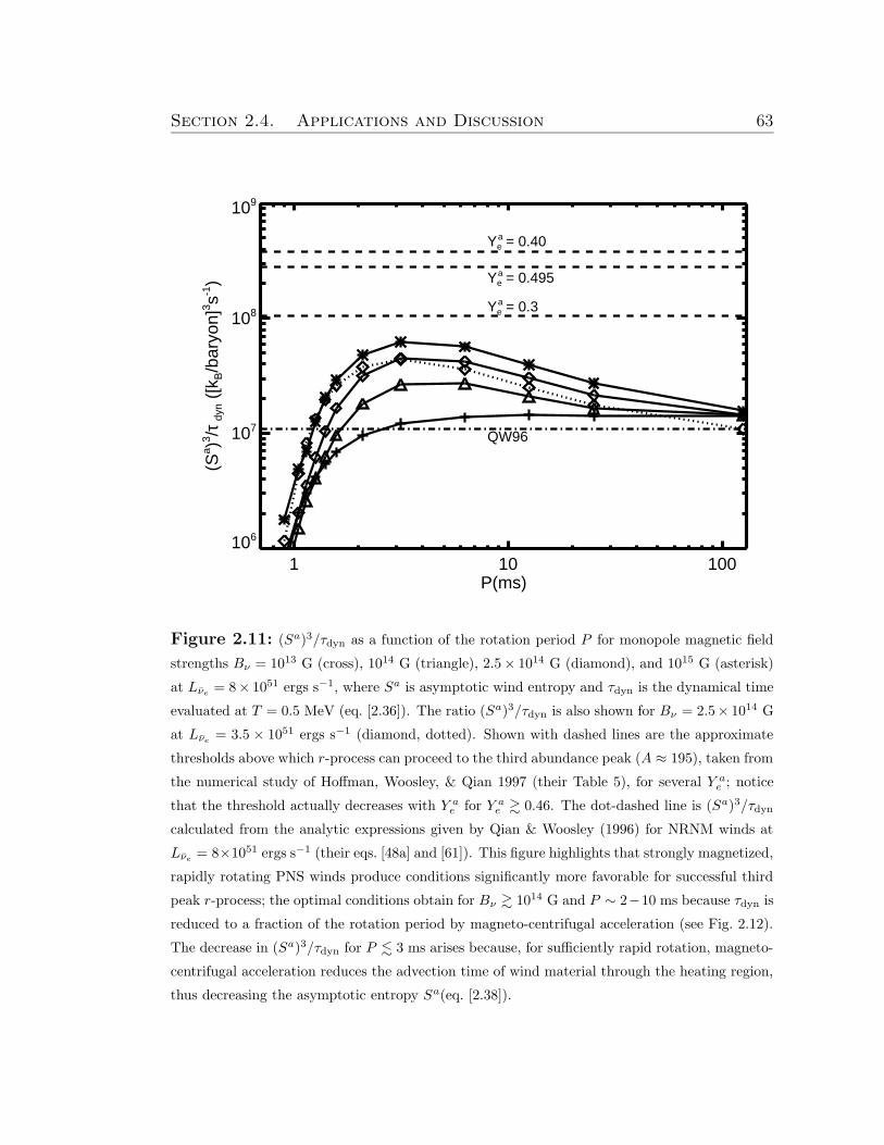
Section 2.4. Applications and Discussion 63
1 10 100P(ms)
106
107
108
109(S
a )3 /τ d
yn (
[kB/b
aryo
n]3 s-1
)
Ye = 0.3a
Ye = 0.495a
Ye = 0.40a
QW96
Figure 2.11: (Sa)3/τdyn as a function of the rotation period P for monopole magnetic field
strengths Bν = 1013 G (cross), 1014 G (triangle), 2.5× 10¹⁴ G (diamond), and 1015 G (asterisk)
at Lνe= 8× 1051 ergs s−1, where Sa is asymptotic wind entropy and τdyn is the dynamical time
evaluated at T = 0.5 MeV (eq. [2.36]). The ratio (Sa)3/τdyn is also shown for Bν = 2.5× 10¹⁴ G
at Lνe= 3.5 × 1051 ergs s−1 (diamond, dotted). Shown with dashed lines are the approximate
thresholds above which r-process can proceed to the third abundance peak (A ≈ 195), taken from
the numerical study of Hoffman, Woosley, & Qian 1997 (their Table 5), for several Y ae ; notice
that the threshold actually decreases with Y ae for Y a
e & 0.46. The dot-dashed line is (Sa)3/τdyn
calculated from the analytic expressions given by Qian & Woosley (1996) for NRNM winds at
Lνe= 8×1051 ergs s−1 (their eqs. [48a] and [61]). This figure highlights that strongly magnetized,
rapidly rotating PNS winds produce conditions significantly more favorable for successful third
peak r-process; the optimal conditions obtain for Bν & 1014 G and P ∼ 2−10 ms because τdyn is
reduced to a fraction of the rotation period by magneto-centrifugal acceleration (see Fig. 2.12).
The decrease in (Sa)3/τdyn for P . 3 ms arises because, for sufficiently rapid rotation, magneto-
centrifugal acceleration reduces the advection time of wind material through the heating region,
thus decreasing the asymptotic entropy Sa(eq. [2.38]).
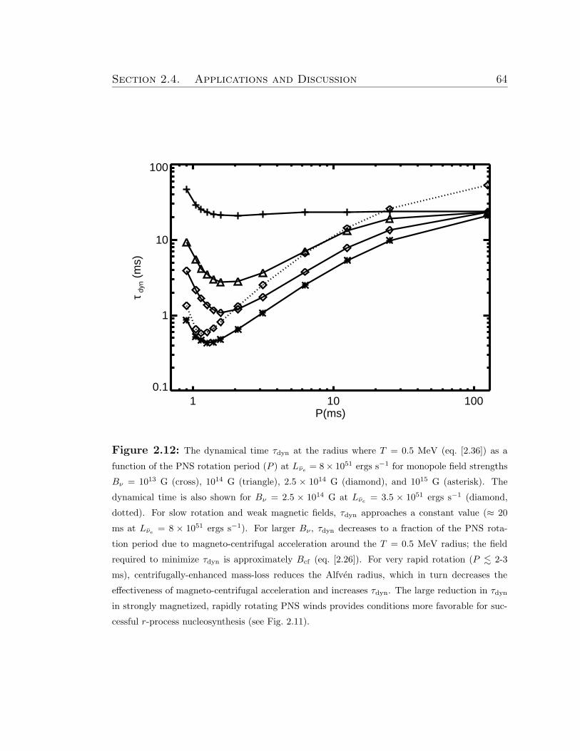
Section 2.4. Applications and Discussion 64
1 10 100P(ms)
0.1
1
10
100
τ dyn
(m
s)
Figure 2.12: The dynamical time τdyn at the radius where T = 0.5 MeV (eq. [2.36]) as a
function of the PNS rotation period (P ) at Lνe= 8× 1051 ergs s−1 for monopole field strengths
Bν = 1013 G (cross), 1014 G (triangle), 2.5 × 10¹⁴ G (diamond), and 1015 G (asterisk). The
dynamical time is also shown for Bν = 2.5 × 10¹⁴ G at Lνe= 3.5 × 1051 ergs s−1 (diamond,
dotted). For slow rotation and weak magnetic fields, τdyn approaches a constant value (≈ 20
ms at Lνe= 8 × 1051 ergs s−1). For larger Bν , τdyn decreases to a fraction of the PNS rota-
tion period due to magneto-centrifugal acceleration around the T = 0.5 MeV radius; the field
required to minimize τdyn is approximately Bcf (eq. [2.26]). For very rapid rotation (P . 2-3
ms), centrifugally-enhanced mass-loss reduces the Alfven radius, which in turn decreases the
effectiveness of magneto-centrifugal acceleration and increases τdyn. The large reduction in τdyn
in strongly magnetized, rapidly rotating PNS winds provides conditions more favorable for suc-
cessful r-process nucleosynthesis (see Fig. 2.11).
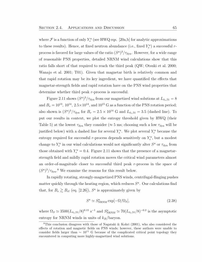
Section 2.4. Applications and Discussion 65
where F is a function of only Y ae (see HWQ eqs. [20a,b] for analytic approximations
to these results). Hence, at fixed neutron abundance (i.e., fixed Y ae ) a successful r-
process is favored for large values of the ratio (Sa)3/τdyn. However, for a wide range
of reasonable PNS properties, detailed NRNM wind calculations show that this
ratio falls short of that required to reach the third peak (QW; Otsuki et al. 2000;
Wanajo et al. 2001; T01). Given that magnetar birth is relatively common and
that rapid rotation may be its key ingredient, we have quantified the effects that
magnetar-strength fields and rapid rotation have on the PNS wind properties that
determine whether third peak r-process is successful.
Figure 2.11 shows (Sa)3/τdyn from our magnetized wind solutions at Lνe,51 = 8
and Bν = 1013, 1014, 2.5×10¹⁴, and 1015 G as a function of the PNS rotation period;
also shown is (Sa)3/τdyn for Bν = 2.5× 10¹⁴ G and Lνe,51 = 3.5 (dashed line). To
put our results in context, we plot the entropy threshold given by HWQ (their
Table 5) at the lowest τdyn they consider (≈ 5 ms; choosing such a low τdyn will be
justified below) with a dashed line for several Y ae . We plot several Y a
e because the
entropy required for successful r-process depends sensitively on Y ae , but a modest
change to Y ae in our wind calculations would not significantly alter Sa or τdyn from
those obtained with Y ae = 0.4. Figure 2.11 shows that the presence of a magnetar-
strength field and mildly rapid rotation moves the critical wind parameters almost
an order-of-magnitude closer to successful third peak r-process in the space of
(Sa)3/τdyn.8 We examine the reasons for this result below.
In rapidly rotating, strongly-magnetized PNS winds, centrifugal-flinging pushes
matter quickly through the heating region, which reduces Sa. Our calculations find
that, for Bν & Bcf (eq. [2.26]), Sa is approximately given by
Sa ' SaNRNM exp[−Ω/ΩS], (2.38)
where ΩS ' 3500(Lνe,51/8)0.15 s−1 and SaNRNM ' 70(Lνe,51/8)
−0.2 is the asymptotic
entropy for NRNM winds in units of kB/baryon.
8This conclusion disagrees with those of Nagataki & Kohri (2001), who also considered theeffects of rotation and magnetic fields on PNS winds; however, these authors were unable toconsider fields larger than ∼ 1011 G because of the complicated critical point topology theyencountered in computing more highly-magnetized wind solutions.
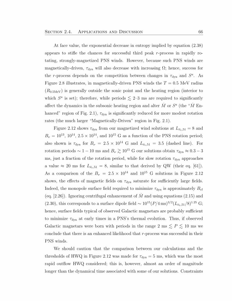
Section 2.4. Applications and Discussion 66
At face value, the exponential decrease in entropy implied by equation (2.38)
appears to stifle the chances for successful third peak r-process in rapidly ro-
tating, strongly-magnetized PNS winds. However, because such PNS winds are
magnetically-driven, τdyn will also decrease with increasing Ω; hence, success for
the r-process depends on the competition between changes in τdyn and Sa. As
Figure 2.8 illustrates, in magnetically-driven PNS winds the T = 0.5 MeV radius
(R0.5MeV) is generally outside the sonic point and the heating region (interior to
which Sa is set); therefore, while periods . 2–3 ms are required to significantly
affect the dynamics in the subsonic heating region and alter M or Sa (the “M En-
hanced” region of Fig. 2.1), τdyn is significantly reduced for more modest rotation
rates (the much larger “Magnetically-Driven” region in Fig. 2.1).
Figure 2.12 shows τdyn from our magnetized wind solutions at Lνe,51 = 8 and
Bν = 1013, 1014, 2.5× 10¹⁴, and 1015 G as a function of the PNS rotation period;
also shown is τdyn for Bν = 2.5 × 10¹⁴ G and Lνe,51 = 3.5 (dashed line). For
rotation periods ∼ 1− 10 ms and Bν & 1015 G our solutions obtain τdyn ≈ 0.3− 3
ms, just a fraction of the rotation period, while for slow rotation τdyn approaches
a value ≈ 20 ms for Lνe,51 = 8, similar to that derived by QW (their eq. [61]).
As a comparison of the Bν = 2.5 × 10¹⁴ and 1015 G solutions in Figure 2.12
shows, the effects of magnetic fields on τdyn saturate for sufficiently large fields.
Indeed, the monopole surface field required to minimize τdyn is approximately Bcf
(eq. [2.26]). Ignoring centrifugal enhancement of M and using equations (2.15) and
(2.30), this corresponds to a surface dipole field ∼ 1015(P/4ms)3/2(Lνe,51/8)1.25 G;
hence, surface fields typical of observed Galactic magnetars are probably sufficient
to minimize τdyn at early times in a PNS’s thermal evolution. Thus, if observed
Galactic magnetars were born with periods in the range 2 ms . P . 10 ms we
conclude that there is an enhanced likelihood that r-process was successful in their
PNS winds.
We should caution that the comparison between our calculations and the
thresholds of HWQ in Figure 2.12 was made for τdyn = 5 ms, which was the most
rapid outflow HWQ considered; this is, however, almost an order of magnitude
longer than the dynamical time associated with some of our solutions. Constraints
Section 2.4. Applications and Discussion 67
similar to HWQ at τdyn ∼ 3ms are obtained by Meyer & Brown (1997). A some-
what different threshold is obtained by Sasaqui et al. (2006), who emphasize a
previously neglected light-element r-process seed production channel. In fact, re-
cent work by Meyer (2002) shows that the threshold for r-process nucleosynthesis
may be modified at very short τdyn compared to standard expectations (i.e., Y ae
must be less than 0.5). In order to accurately assess whether r-process nucle-
osynthesis in proto-magnetar winds will proceed to the third abundance peak and
beyond, or whether the nucleosynthesis that results from these outflows may be
used to constrain the birth rate of proto-magnetars, a survey of nucleosynthesis
calculations should be carried out at short τdyn. In fact, the critical question of
whether this modest Sa, very-low τdyn mode of r-process can reproduce the seem-
ingly universal solar abundance curve above Ba (e.g., Cowan et al. 2005) must
ultimately be answered through detailed nucleosynthesis calculations on our wind
solutions (such calculations are currently in progress) and by including a better
treatment of Ye in the wind. The effects of GR not included in our calculations
will tend to increase Sa and Y ae , on balance probably increasing the likelihood of
successful r-process (Fuller & Qian 1996; Cardall & Fuller 1997).
T01 found that in NRNM winds Sa ∝ (τdyn)0.2; thus, even though Sa ∝ L−0.2νe
increases with time as the PNS cools, it is difficult for a NRNM wind that does
not produce conditions favorable for third peak r-process (eq. [2.37]) at early times
to enter the regime for a successful r-process at later times. We might expect
a modification to the PNS (Sa, τdyn) evolutionary track in the case of a proto-
magnetar because the dynamical time in a magnetically-driven PNS wind is no
longer set solely by the neutrino heating. In order to address this question, we
explored how (Sa)3/τdyn changes as the PNS cools. As shown in Figure 2.11, from
our calculations at Lνe,51 = 3.5 and Bν = 2.5 × 10¹⁴ G we find that (Sa)3/τdyn
changes by less than a factor of 2 from those at Lνe,51 = 8 and Bν = 2.5 × 10¹⁴
G; in particular, the peak value of (Sa)3/τdyn at P ∼ 3 ms remains essentially
unchanged. Thus the conditions for r-process in magnetically-driven PNS winds
do not vary strongly with luminosity over the range we have explored.
To conclude this section, we briefly consider what constraints can be placed on
Section 2.4. Applications and Discussion 68
r-process in proto-magnetar winds if they are to be capable of having a significant
effect on the heavy element abundance evolution of the Galaxy. If most SNe
produce r-process elements, the total r-process-rich wind mass ejected per SN
must be ∼ 10−6 − 10−5 M¯ to account for the total Galactic yield (e.g., Qian
2000); hence, because the magnetar birthrate is ∼ 10% of the total neutron star
birthrate, at least ∼ 10−5−10−4 M¯ of r-process-rich material must be ejected per
magnetar birth (this number is quite uncertain because the magnetar birthrate is
uncertain; see Woods & Thompson 2004). Because r-process in proto-magnetar
winds is only likely to be successful for P & 2−3 ms, rotation does not significantly
enhance mass-loss from the PNS (Fig. 2.10). As a result, the required yield of r-
process rich material per magnetar birth is similar to our estimates for the total
mass extracted in NRNM PNS winds (∼ 10−4 M¯). Thus we conclude that if
proto-magnetar winds are the dominant source for Galactic r-process, the r-process
probably must occur early in the PNS cooling evolution (in the first few seconds,
even earlier than for normal PNSs)9. The former in part justifies our concentration
on high Lνe in Figure 2.11 and means that the question of whether magnetar birth
is a significant source for Galactic r-process is especially sensitive to the early
evolution of the magnetic field and radius of the PNS.
It is also worth noting that on the basis of a comparison between the solar
r-process abundance pattern with meteoritic abundances of 129I and 182Hf, Qian,
Vogel, & Wasserburg (1998) (see also Wasserburg et al. 1996) suggest a diversity
of r-process sites. In particular, they argue for a site with high frequency (roughly
the Galactic SN rate) that generates the A ≈ 195 nuclei and a site 10 times less
frequent that produces nuclei near A ≈ 135. In order to satisfy the observational
constraints, the latter site must eject 10 times the mass of the high-frequency site,
per event. Although we have not proven that magnetars produce an r-process
in any mass range the ∼ 10% birth fraction of magnetars, the characteristically
larger total ejected mass (Fig. [2.10]), and the very different thermodynamics of
their winds relative to NRNM PNS winds make it tempting to associate proto-
9Of course, if the magnetar birthrate has been underestimated and is comparable to the totalNS birthrate then r-process could occur somewhat later in the PNS evolution.
Section 2.4. Applications and Discussion 69
magnetar winds with the low-frequency enrichment events advocated by Qian,
Vogel & Wasserburg (1998).
Wave Heating
QW show that by including a heating source in addition to neutrinos outside
a few PNS radii, the wind entropy is increased, the dynamical time is reduced,
and the chances for a successful r-process can be substantially improved. Such an
extended heating mechanism operates above the sun, where convectively excited
waves are believed to heat the extended solar corona (for recent work see Cranmer
& van Ballegooijen 2005). The neutrino cooling luminosity of a PNS also drives
vigorous convection during the Kelvin-Helmholtz epoch (e.g., Burrows & Lattimer
1986; Burrows, Hayes, & Fryxell 1995). It is likely that a fraction of the convective
energy flux will be deposited into outgoing waves, which will then propagate into
the PNS atmosphere and deposit their energy and momentum on a length scale
of order a few PNS radii. The relative importance of hydrodynamic and MHD
wave excitation likely depends on the magnetic field strength of the PNS. Here
we focus on heating by MHD waves in the magnetospheres of strongly magnetized
PNSs (Suzuki & Nagataki 2005), though hydrodynamic wave excitation may be
important as well (e.g., Burrows et al. 2006a,b). If the energy flux in MHD waves
at the PNS surface is Fw(Rν) = (1/2)ρv3A(δB/Br)2|Rν , we estimate that the total
wave heating Qw ≈ 4πR2νFw(Rν) is given by
Qw ' 1048(B15)3
(
δBν/Bν
0.1
)2
ergs s−1, (2.39)
where δBν ≡ δB(Rν) is the amplitude of the waves excited at the PNS surface
(with a density ρ(Rν) ≈ 1012 g cm−3). The ratio of the wave heating in equation
(2.39) to the total neutrino heating Qν = 4π∫∞
Rνr2ρqνdr in the absence of rotation
can be approximated as
Qw
Qν
≈ 0.03(B15)3
(
δBν/Bν
0.1
)2(Lνe,518
)−2.8
, (2.40)
where Qν ≈ 4.4× 1049(Lνe,51/8)2.8 ergs s−1 is taken from our NRNM calculations
and agrees reasonably well with the results of T01 (their Table 1). Equation
Section 2.4. Applications and Discussion 70
(2.40) illustrates that, for efficient wave excitation, wave heating at early times
may become important for field strengths & 1014 − 1015 G. Equation (2.40) also
appears to suggest that wave heating will become substantially more important
as the PNS cools and Lνe drops; however, whether this in fact occurs is unclear
because the energy flux in waves and the surface amplitude δBν will likely decrease
with Lνe as the convective flux decreases.
In order to quantify the effects that wave heating have on the entropy and
dynamical time in rotating PNS winds, we consider a concrete model in which we
add Alfven wave pressure and heating to our solutions. In the entropy equation
(eq. [2.9]), this leads to an additional source term of the form
qw(r) =vA
vr + vA
Fw(Rν)
χRνρ
(
Rν
r
)2
exp
[
−(r −Rν)
χRν
]
, (2.41)
where the factor vA/(vr+vA) < 1 accounts for the work done by the Alfven waves.
Equation (2.41) concentrates the total wave heating (Qw = 4π∫∞
Rνr2ρqwdr) on a
radial length scale ≈ χRν . Radially propagating Alfven waves also exert a pressure
on the fluid (Pw), which contributes a term to the right hand side of the radial
momentum equation (eq. [2.3]) of the form (Lamers & Cassinelli 1999; Suzuki &
Nagataki 2005)
−1
ρ
dPw
dr=
qw2(vr + vA)
−(δB)2
32πρ
3vr + vAvr + vA
1
ρ
dρ
dr, (2.42)
where
(δB)2 =8πχRνρqwvr + vA
. (2.43)
We consider a variety of dissipation lengths (Rνχ) and surface wave amplitudes
(δBν) and assess the effects of Alfven wave heating on our wind solutions. For
reasons discussed at the end of §2.4.3, we are primarily interested in the effect
that wave heating has on r-process at early times; thus, we concentrate on wave
heating applied to high luminosity solutions.
Our wave heating calculations are summarized in Table 2.3. Motivated by the
r-process threshold of HWQ (eq. [2.37]), we quantify the improvement towards a
Section 2.4. Applications and Discussion 71
successful r-process through an “improvement factor”:
Iw(Qw, χ) ≡[S3
0.5MeV/τdyn]Qw
[S30.5MeV/τdyn]Qw=0
, (2.44)
where S0.5MeV is the entropy at the radius where T = 0.5 MeV. Figure 2.11 shows
that for Lνe,51 = 8, Bν = 1015 G, and P = 3 ms (corresponding to the peak
in Fig. 2.11) an improvement factor Iw & 6 is required to exceed the HWQ
threshold for third-peak r-process for Y ae ≈ 0.4, while for a NRNM solution at
Lνe,51 = 8 successful r-process requires Iw & 25. We should note, however, that
HWQ assumed adiabatic expansion through the α-process temperature range (T ≈
0.5− 0.2 MeV), while for large χ wave heating is important at these radii and the
expansion is not adiabatic. This may modify the Iw required for successful r-
process.
For P ' 3(130) ms, B = 1015 G, and Lνe,51 = 8, we find that Iw & 6(25)
requires an amplitude δBν/Bν & 0.5− 0.7 and a dissipation length χ ∼ 3.10 This
wave amplitude corresponds to a total wave heating & 4 × 1049 ergs s−1, which
is comparable to the total neutrino heating for this solution and is ∼ 10−3 of the
neutrino luminosity at early times. The fact that a comparable wave energy is
required in the slow and rapidly rotating limits appears somewhat coincidental.
For the non-rotating solutions, the wave heating only reduces the dynamical time
to ∼ 2 ms, never reaching the regime of τdyn . 1 ms obtained in rotating PNS
winds. The entropy increase at T = 0.5 MeV is, however, larger in the non-rotating
case because the T = 0.5 MeV radius is at larger radii (and thus S0.5MeV is closer
to Sa). Although the actual wave dissipation mechanism in the PNS atmosphere
is uncertain, we note that for initial amplitudes of δBν/Bν ∼ 0.5, conservation of
action implies that the waves are nonlinear with δB/Br ∼ 1 at ∼ 3− 4Rν , similar
to the dissipation lengths (χ) that are optimal for r-process. Also note that for
more rapidly rotating solutions (P ≈ 1 ms), significantly more wave heating is
10For very small χ, the wave heating effectively acts as an increase to the neutrino luminosity,which decreases the asymptotic entropy Sa (recall that – absent wave heating – the entropydecreases with increasing luminosity). For large χ, on the other hand, the heating is concentratedoutside the T = 0.5 MeV radius and, while Sa increases substantially, the entropy at T = 0.5MeV remains relatively unaffected.
Section 2.4. Applications and Discussion 72
required for successful r-process: even δBν ≈ Bν is insufficient at B ≈ 1015 G.
This is because the total neutrino heating itself increases at P ∼ 1 ms (ρ is larger
in the neutrino heating region due to magneto-centrifugal support), so a given
amount of wave heating has less of an effect on the solution.
For lower neutrino luminosities, smaller Qw can lead to successful r-process.
For example, at Lνe,51 = 3.5 and B = 2.5 × 10¹⁴ G, we find that, for P = 3(130)
ms, Qw & 1049(5 × 1048) ergs s−1 and χ ∼ 3 is required to eclipse the HWQ r-
process threshold for Y ae = 0.4.11 The required wave heating in this case is again
comparable to the total neutrino heating, but is only ∼ 6× 10⁻⁴(3× 10⁻⁴) of the
neutrino luminosity of the PNS. At even lower Lν , a yet smaller fraction of the neu-
trino luminosity in wave heating would be capable of yielding successful r-process.
However, as discussed in the previous section, constraints on the r-process rich
material required per magnetar-birth imply that the r-process must be successful
at relatively high neutrino luminosities. We thus conclude that wave heating leads
to successful r-process if & 10−4 − 10−3 of the PNS’s neutrino luminosity emerges
in wave power at early times in the Kelvin Helmholtz epoch, and that this re-
quired level of wave heating is essentially independent of magnetic field strength
and rotation rate (for P & 2 ms).
Although the mechanism and formula we describe here are appropriate to
proto-magnetars with large magnetic fields, it is possible that hydrodynamic (as
opposed to MHD) wave heating is important and generic to normal PNS birth. In
this case, waves may be generated by convective motions as the PNS cools, or via
global modes of the PNS similar to those observed by Burrows et al. (2006a,b), that
persist into the cooling epoch. As in the MHD case, a fraction of the total neutrino
luminosity (10−4−10−3) must emerge in wave power over τKH to produce conditions
suitable for the r-process. Because such a mechanism may operate generically (and
11Suzuki & Nagataki (2005) found that for non-rotating solutions with Alfven wave heating,r-process was successful for Qw ' 2×1048 ergs s−1 and χ ∼ 5−10 at Lνe,51 ∼ 1. Our results aresimilar to theirs although their required wave heating is somewhat larger than an extrapolationof our results would suggest. However, they used different mean neutrino energies than we haveassumed and obtain M ∼ 2 × 10⁻⁶ M¯ s−1, roughly 3 times greater than we predict fromequation (2.15) at Lνe,51 = 1. This larger mass-loading may explain why their calculationsrequired somewhat more wave heating to enter the regime of successful r-process.
Section 2.4. Applications and Discussion 73
not just in proto-magnetars) the requirement of an early-time r-process highlighted
above for the proto-magnetars and in §4.3 is somewhat alleviated.
2.4.4 Additional Applications
While most magnetar formation probably results from the core collapse of
a massive star, magnetars may also form through the accretion-induced collapse
(AIC) of a white dwarf (Nomoto et al. 1979; Usov 1992; Woosley & Baron 1992).
Rapid rotation will automatically accompany AIC due to the accretion of mass
and angular momentum prior to collapse, and a strong field may accompany the
final stages of the contraction of the PNS, amplified through either magnetic flux-
freezing of the progenitor white dwarf’s field or via dynamo action (Duncan &
Thompson 1992). The properties of PNSs formed following AIC would thus be
very similar to those of the proto-magnetars that we have considered in this pa-
per and the resulting proto-magnetar wind would be accurately modeled using
our calculations. AIC may thus give rise to a LGRB with properties similar to
those considered in §2.4.2. However, LGRBs from AIC will not produce significant
amounts of Ni (Woosley & Baron 1992; Dessart et al. 2006) and hence will not
be associated with a simultaneous hyper-energetic Type-Ic SN, as in, e.g. GRB
980425/SN1998bw or GRB 030329/2003dh (Galama et al. 1998; Hjorth et al. 2003;
Stanek et al. 2003; Woosley & Bloom 2006). Instead, AIC should be associated
with a class of SN-less LGRBs like GRB 060505 and 060614 (Fynbo et al. 2006;
Gal-Yam et al. 2006; Della Valle et al. 2006). A prediction of this model is that
these LGRBs should be associated with both relatively old (few Gyr) and rela-
tively young (∼100Myr) stellar populations. If some SN-less LGRBs are found
to be associated with old stellar populations, it would strongly support the AIC
interpretation.
Although we have focused on magnetized PNS evolution in this paper, the
physical conditions we have considered are quite similar to those expected in a
neutrino-cooled accretion disk surrounding a newly-formed black hole in the “col-
lapsar” model for LGRBs (Woosley 1993; Paczynski 1998; MacFadyen & Woosley
Section 2.5. Conclusions 74
1999). For concreteness, consider the properties of a thin accretion disk with an ac-
cretion rate Macc = 0.2M¯ s−1 and viscosity parameter α = 0.01 at a fiducial radius
of ≈ 100 km, or approximately 10 Schwarzschild radii above a non-rotating black
hole of mass 3M¯. According to the calculations of Chen & Beloborodov (2006), at
these radii (where P ≈ 10 ms) the disk is optically thick to neutrinos, the surface
temperature of the disk is very similar to that of a PNS neutrinosphere (≈ 2 − 3
MeV), and the total neutrino luminosity of the disk is Lν ' 0.04Maccc2 ≈ 1.4×1052
ergs s−1 (their Fig. 18), comparable to that of a PNS at early times (note that
at lower accretion rates the disk will be optically thin to neutrinos). If this disk
were threaded with a large-scale poloidal field with a strength corresponding to
that expected for MRI turbulence, B ≈ 1014 − 1015 G (plasma β ≈ 10− 100), the
physical conditions would indeed resemble those in proto-magnetar winds. Thus
neutrino-magneto-centrifugal driving may be important in setting the mass-loading
and energy-loss rate in outflows from collapsar disks. Indeed, Levinson (2006) has
calculated the mass loading of neutrino-driven outflows in general relativistic MHD
for conditions anticipated in collapsar disks, finding qualitatively similar results to
those discussed in this paper for PNS winds.
As a final context in which our calculations may be relevant, we note that
a magnetized accretion flow like that considered above for collapsars or a short-
lived, rapidly rotating proto-magnetar may be formed following the merger of a
NS-NS binary (Paczynski 1986; Eichler et al. 1989; Rosswog & Liebendorfer 2003).
Our calculations would also describe magnetized outflow from these objects, but
additional work is needed to explore this application in more detail.
2.5 Conclusions
We have solved the one-dimensional non-relativistic neutrino-heated MHD
wind problem in order to study the effects that magnetic fields and rotation have
on PNS wind evolution following the launch of the SN shock but prior to the
end of the Kelvin-Helmholtz cooling epoch. Figure 2.1 summarizes the physical
regimes of PNS winds in the presence of rotation and magnetic fields. We map
Section 2.5. Conclusions 75
our monopole solutions onto the axisymmetric, relativistic dipole calculations of
B06, thus taking into account the effects that neutrino-driven mass-loss have on
the fraction of open magnetic flux and the PNS spin-down rate. Our primary
conclusions are as follows:
• We identify three types of PNSs based on the dominant character of their
energy-loss during the Kelvin-Helmholtz epoch (see Figure 2.9):
(1) For slow rotation and low magnetic field strengths (Bdip14 . 10−2P 2
ms,
where Bdip = 1014Bdip14 G is the surface dipole field strength of the PNS
and P = 1Pms ms is its birth period), a neutrino-heated, thermally-
driven wind dominates energy and mass-loss from the PNS; most radio
pulsars were probably this type at birth.
(2) For larger rotation rates and field strengths
(10−2P 2ms . Bdip
14 . 2P 2ms exp[2P
−2ms ]), a non-relativistic, magnetically-
driven wind dominates during the Kelvin-Helmholtz epoch. Most ob-
served Galactic magnetars (∼ 10% the birthrate of radio pulsars) were
probably of this type at birth. For B ∼ 1015 G and P . 2 ms, greater
than 1051 ergs can be lost to a non-relativistic, magnetically-driven out-
flow during τKH , and, over a broad range of initial spin period, the en-
ergy extracted is many times larger than from a slowly rotating PNS
(see Fig. 2.9). The outflow from this type of PNS is likely to be colli-
mated by magnetic stresses and the asymmetric injection of energy may
be sufficient to generate an anisotropy in the morphology of the SNe
remnant.
(3) For rapid rotation and field strengths somewhat larger than those ob-
served from Galactic magnetars (Bdip14 & 2P 2
ms exp[2P−2ms ]), a relativis-
tic, magnetically-driven wind dominates energy-loss during the Kelvin-
Helmholtz epoch. Although the birthrate of PNSs of this type is proba-
bly small (if they are produced at all), they may be capable of producing
hyper-energetic SNe and long-duration gamma-ray bursts.
Section 2.5. Conclusions 76
• For P ≈ 3(1) ms and Bdipν & 1015 G the total mass-loss during the Kelvin-
Helmholtz epoch is enhanced by a factor of≈ 2(102) relative to a non-rotating
PNS (Fig. 2.10).
• For initial PNS spin periods of P ≈ 1 ms and magnetic field strengths of
Bdipν ≈ 3 × 10¹⁵ − 1016 G, we find that & 1052 ergs of rotational energy
is extracted on a timescale of 10 − 40 seconds and that the magnetization
σ of the outflow is ∼ 0.1 − 1000. The energy, luminosity, timescale, and
mass-loading of the late-time outflow are all consistent with those required
to explain long duration gamma-ray bursts (assuming efficient dissipation of
magnetic energy into kinetic energy at large radii; e.g., Drenkhahn & Spruit
2002). In addition, outflows from such PNSs have the property that the PNS
rotational energy is extracted with a roughly uniform distribution in log(σ)
over the timescale τKH. For these modest σ winds, especially at early times,
energy-loss from the PNS is enhanced relative to pure force-free spindown
because of additional open magnetic flux (see the discussion in §2.4.1). Thus,
a significant portion of the PNS rotational energy can be extracted in just a
few seconds following the launch of the SN shock, perhaps sufficiently rapidly
to increase the nucleosynthetic yield of the SN (e.g., 56Ni).
• Winds from PNSs with Bdipν & 1015 G and P ≈ 2 − 10 ms produce condi-
tions almost an order-of-magnitude more favorable for third-peak r-process
nucleosynthesis in the space of (Sa)3/τdyn than do winds from more slowly-
rotating, less-magnetized PNSs (see Fig. 2.11). For these rotation rates,
the asymptotic entropy is similar to that of a non-rotating, non-magnetized
wind, while the dynamical time is significantly reduced by magnetic accelera-
tion (see Fig. 2.12). The very different thermodynamic properties of rapidly
rotating proto-magnetar winds (relative to non-rotating PNS winds) may
contribute to the inferred diversity of r-process sites (e.g., Qian et al. 1998).
• Heating by outgoing hydrodynamic or MHD waves may be important in
PNS winds. We find that if & 10−4 − 10−3 of the PNS’s neutrino luminosity
Section 2.5. Conclusions 77
emerges in wave power at early times in the Kelvin-Helmholtz epoch, then r-
process is successful in PNS winds. This conclusion is relatively independent
of magnetic field strength and rotation period for P & 2 ms.
Acknowledgements
We thank Niccolo Bucciantini and Jon Arons for helpful discussions. We also thank
Martin White and Marc Davis for computational time on their Beowulf cluster.
T.A.T. thanks the Aspen Center for Physics, where this work germinated, for its
hospitality. EQ and BDM were supported in part by NSF grant AST 0206006,
NASA grants NAG5-12043 and NNG05GO22H, an Alfred P. Sloan Fellowship, the
David and Lucile Packard Foundation, and a NASA GSRP Fellowship to BDM.
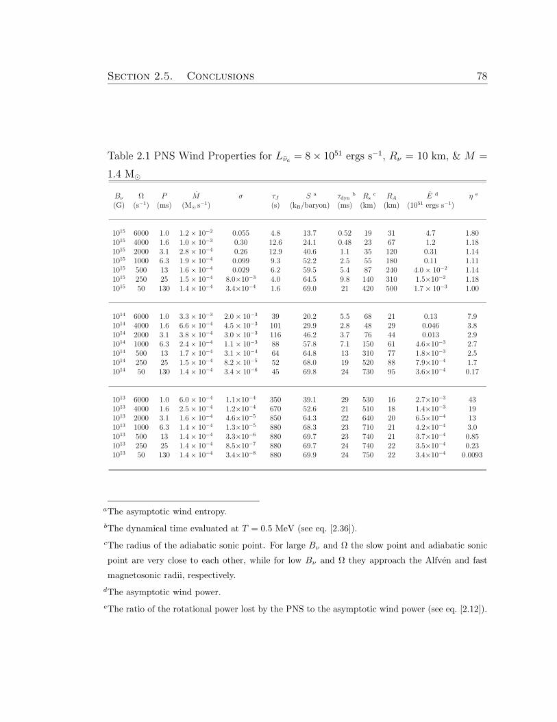
Section 2.5. Conclusions 78
Table 2.1 PNS Wind Properties for Lνe = 8× 1051 ergs s−1, Rν = 10 km, & M =
1.4 M¯
Bν Ω P M σ τJ S a τdynb Rs
c RA E d η e
(G) (s−1) (ms) (M¯ s−1) (s) (kB/baryon) (ms) (km) (km) (1051 ergs s−1)
1015 6000 1.0 1.2× 10⁻² 0.055 4.8 13.7 0.52 19 31 4.7 1.801015 4000 1.6 1.0× 10⁻³ 0.30 12.6 24.1 0.48 23 67 1.2 1.181015 2000 3.1 2.8× 10⁻⁴ 0.26 12.9 40.6 1.1 35 120 0.31 1.141015 1000 6.3 1.9× 10⁻⁴ 0.099 9.3 52.2 2.5 55 180 0.11 1.111015 500 13 1.6× 10⁻⁴ 0.029 6.2 59.5 5.4 87 240 4.0× 10⁻² 1.141015 250 25 1.5× 10⁻⁴ 8.0×10⁻³ 4.0 64.5 9.8 140 310 1.5×10⁻² 1.181015 50 130 1.4× 10⁻⁴ 3.4×10⁻⁴ 1.6 69.0 21 420 500 1.7× 10⁻³ 1.00
1014 6000 1.0 3.3× 10⁻³ 2.0× 10⁻³ 39 20.2 5.5 68 21 0.13 7.91014 4000 1.6 6.6× 10⁻⁴ 4.5× 10⁻³ 101 29.9 2.8 48 29 0.046 3.81014 2000 3.1 3.8× 10⁻⁴ 3.0× 10⁻³ 116 46.2 3.7 76 44 0.013 2.91014 1000 6.3 2.4× 10⁻⁴ 1.1× 10⁻³ 88 57.8 7.1 150 61 4.6×10⁻³ 2.71014 500 13 1.7× 10⁻⁴ 3.1× 10⁻⁴ 64 64.8 13 310 77 1.8×10⁻³ 2.51014 250 25 1.5× 10⁻⁴ 8.2× 10⁻⁵ 52 68.0 19 520 88 7.9×10⁻⁴ 1.71014 50 130 1.4× 10⁻⁴ 3.4× 10⁻⁶ 45 69.8 24 730 95 3.6×10⁻⁴ 0.17
1013 6000 1.0 6.0× 10⁻⁴ 1.1×10⁻⁴ 350 39.1 29 530 16 2.7×10⁻³ 431013 4000 1.6 2.5× 10⁻⁴ 1.2×10⁻⁴ 670 52.6 21 510 18 1.4×10⁻³ 191013 2000 3.1 1.6× 10⁻⁴ 4.6×10⁻⁵ 850 64.3 22 640 20 6.5×10⁻⁴ 131013 1000 6.3 1.4× 10⁻⁴ 1.3×10⁻⁵ 880 68.3 23 710 21 4.2×10⁻⁴ 3.01013 500 13 1.4× 10⁻⁴ 3.3×10⁻⁶ 880 69.7 23 740 21 3.7×10⁻⁴ 0.851013 250 25 1.4× 10⁻⁴ 8.5×10⁻⁷ 880 69.7 24 740 22 3.5×10⁻⁴ 0.231013 50 130 1.4× 10⁻⁴ 3.4×10⁻⁸ 880 69.9 24 750 22 3.4×10⁻⁴ 0.0093
aThe asymptotic wind entropy.
bThe dynamical time evaluated at T = 0.5 MeV (see eq. [2.36]).
cThe radius of the adiabatic sonic point. For large Bν and Ω the slow point and adiabatic sonic
point are very close to each other, while for low Bν and Ω they approach the Alfven and fast
magnetosonic radii, respectively.
dThe asymptotic wind power.
eThe ratio of the rotational power lost by the PNS to the asymptotic wind power (see eq. [2.12]).
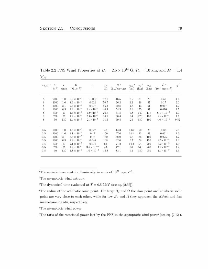
Section 2.5. Conclusions 79
Table 2.2 PNS Wind Properties at Bν = 2.5× 10¹⁴ G, Rν = 10 km, and M = 1.4
M¯
Lνe,51a Ω P M σ τJ S b τdyn
c Rsd RA E e η f
(s−1) (ms) (M¯ s−1) (s) (kB/baryon) (ms) (km) (km) (1051 ergs s−1)
8 6000 1.0 6.2× 10⁻³ 0.0067 17.0 16.5 2.2 31 23 0.57 4.18 4000 1.6 8.3× 10⁻⁴ 0.022 50.7 26.2 1.1 28 37 0.17 2.08 2000 3.1 2.6× 10⁻⁴ 0.017 56.3 42.8 1.8 43 61 0.047 1.78 1000 6.3 1.8× 10⁻⁴ 6.4×10⁻³ 40.4 54.3 3.8 75 87 0.016 1.78 500 13 1.5× 10⁻⁴ 1.9×10⁻⁴ 26.7 61.8 7.8 140 117 6.1× 10⁻³ 1.78 250 25 1.4× 10⁻⁴ 5.0×10⁻⁴ 18.1 66.4 14 270 150 2.4×10⁻³ 1.68 50 130 1.4× 10⁻⁴ 2.1×10⁻⁵ 11.6 69.5 23 680 190 4.6× 10⁻⁴ 0.52
3.5 6000 1.0 1.6× 10⁻³ 0.027 47 14.3 0.66 20 28 0.37 2.33.5 4000 1.6 1.1× 10⁻⁴ 0.17 150 27.6 0.81 23 57 0.091 1.33.5 2000 3.1 3.6× 10⁻⁵ 0.13 152 48.0 2.5 36 100 0.025 1.23.5 1000 6.3 2.4× 10⁻⁵ 0.048 108 62.0 6.7 58 150 8.5×10⁻³ 1.23.5 500 13 2.1× 10⁻⁵ 0.014 69 71.2 14.3 94 200 3.2×10⁻³ 1.33.5 250 25 1.9× 10⁻⁵ 3.8× 10⁻³ 43 77.1 26 160 260 1.2×10⁻³ 1.43.5 50 130 1.8× 10⁻⁵ 1.6× 10⁻⁴ 15.8 83.1 53 550 450 1.1×10⁻⁴ 1.5
aThe anti-electron neutrino luminosity in units of 1051 ergs s−1.
bThe asymptotic wind entropy.
cThe dynamical time evaluated at T = 0.5 MeV (see eq. [2.36]).
dThe radius of the adiabatic sonic point. For large Bν and Ω the slow point and adiabatic sonic
point are very close to each other, while for low Bν and Ω they approach the Alfven and fast
magnetosonic radii, respectively.
eThe asymptotic wind power.
fThe ratio of the rotational power lost by the PNS to the asymptotic wind power (see eq. [2.12]).
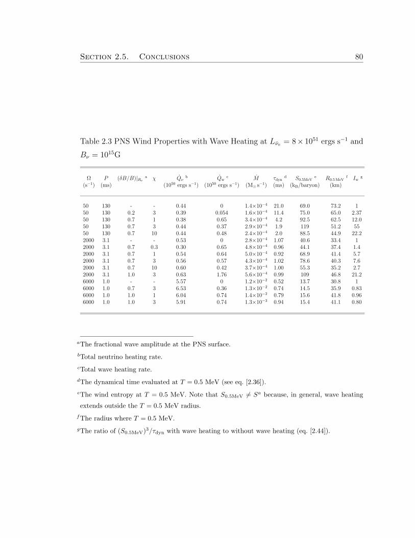
Section 2.5. Conclusions 80
Table 2.3 PNS Wind Properties with Wave Heating at Lνe = 8× 1051 ergs s−1 and
Bν = 1015G
Ω P (δB/B)|Rνa χ Qν
b Qwc M τdyn
d S0.5MeVe R0.5MeV
f Iwg
(s−1) (ms) (1050 ergs s−1) (1050 ergs s−1) (M¯ s−1) (ms) (kB/baryon) (km)
50 130 - - 0.44 0 1.4×10⁻⁴ 21.0 69.0 73.2 150 130 0.2 3 0.39 0.054 1.6×10⁻⁴ 11.4 75.0 65.0 2.3750 130 0.7 1 0.38 0.65 3.4×10⁻⁴ 4.2 92.5 62.5 12.050 130 0.7 3 0.44 0.37 2.9×10⁻⁴ 1.9 119 51.2 5550 130 0.7 10 0.44 0.48 2.4×10⁻⁴ 2.0 88.5 44.9 22.22000 3.1 - - 0.53 0 2.8×10⁻⁴ 1.07 40.6 33.4 12000 3.1 0.7 0.3 0.30 0.65 4.8×10⁻⁴ 0.96 44.1 37.4 1.42000 3.1 0.7 1 0.54 0.64 5.0×10⁻⁴ 0.92 68.9 41.4 5.72000 3.1 0.7 3 0.56 0.57 4.3×10⁻⁴ 1.02 78.6 40.3 7.62000 3.1 0.7 10 0.60 0.42 3.7×10⁻⁴ 1.00 55.3 35.2 2.72000 3.1 1.0 3 0.63 1.76 5.6×10⁻⁴ 0.99 109 46.8 21.26000 1.0 - - 5.57 0 1.2×10⁻² 0.52 13.7 30.8 16000 1.0 0.7 3 6.53 0.36 1.3×10⁻² 0.74 14.5 35.9 0.836000 1.0 1.0 1 6.04 0.74 1.4×10⁻² 0.79 15.6 41.8 0.966000 1.0 1.0 3 5.91 0.74 1.3×10⁻³ 0.94 15.4 41.1 0.80
aThe fractional wave amplitude at the PNS surface.
bTotal neutrino heating rate.
cTotal wave heating rate.
dThe dynamical time evaluated at T = 0.5 MeV (see eq. [2.36]).
eThe wind entropy at T = 0.5 MeV. Note that S0.5MeV 6= Sa because, in general, wave heating
extends outside the T = 0.5 MeV radius.
fThe radius where T = 0.5 MeV.
gThe ratio of (S0.5MeV)3/τdyn with wave heating to without wave heating (eq. [2.44]).
81
Chapter 3
Short GRBs with Extended
Emission from Proto-Magnetar
Spin-Down
B. D. Metzger, E. Quataert, T. A. Thompson (2008), MNRAS, 385, 1455-1460.1
Abstract
Evidence is growing for a class of gamma-ray bursts (GRBs) characterized by
an initial ∼ 0.1 − 1 s spike of hard radiation followed, after a ∼ 3 − 10 s lull in
emission, by a softer period of extended emission lasting ∼ 10 − 100 s. In a few
well-studied cases, these “short GRBs with extended emission” show no evidence
for a bright associated supernova (SN). We propose that these events are produced
by the formation and early evolution of a highly-magnetized, rapidly-rotating neu-
tron star (a “proto-magnetar”) which is formed from the accretion-induced collapse
(AIC) of a white dwarf (WD), the merger and collapse of a WD-WD binary, or,
perhaps, the merger of a double neutron star binary. The initial emission spike is
powered by accretion onto the proto-magnetar from a small disk that is formed
during the AIC or merger event. The extended emission is produced by a relativis-
1Copyright 2008. Royal Astronomical Society. All rights reserved.
Section 3.1. Introduction 82
tic wind that extracts the rotational energy of the proto-magnetar on a timescale
∼ 10− 100 s. The ∼ 10 s delay between the prompt and extended emission is the
time required for the newly-formed proto-magnetar to cool sufficiently that the
neutrino-heated wind from its surface becomes ultra-relativistic. Because a proto-
magnetar ejects little or no 56Ni (< 10−3M¯), these events should not produce a
bright SN-like transient. We model the extended emission from GRB 060614 using
spin-down calculations of a cooling proto-magnetar, finding reasonable agreement
with observations for a magnetar with an initial rotation period of ∼ 1 ms and
a surface dipole field of ∼ 3 × 10¹⁵ G. If GRBs are indeed produced by AIC or
WD-WD mergers, they should occur within a mixture of both early and late-type
galaxies and should not produce strong gravitational wave emission. An addi-
tional consequence of our model is the existence of X-ray flashes unaccompanied
by a bright SN and not associated with massive star formation.
3.1 Introduction
Swift and HETE-2 have demonstrated that long- and short-duration gamma-
ray bursts (GRBs) originate from distinct stellar progenitors. Long GRBs track
ongoing star formation and result from the death of massive stars (Stanek et
al. 2003). On the other hand, short GRBs have now been localized to both early
and late-type host galaxies of moderate redshift (Barthelmy et al. 2005; Berger et
al. 2005; Bloom et al. 2006), indicating a more evolved progenitor population.
Even among the classes of “long” and “short” GRBs, however, diversity is
emerging. One example is GRB 060505 detected by the Burst Alert Telescope
(BAT) on-board Swift. This long-duration burst showed no evidence for a bright
supernova (SN) despite residing inside a star-forming region (Ofek et al. 2007;
Fynbo et al. 2007), suggesting that it may result from a “failed-SN” collapsar
(Woosley 1993). Another particularly striking example is GRB 060614, which,
although officially classified as a long-duration burst based solely on its 102 s T90
duration, more closely resembles a standard short GRB in other ways. This Swift
burst showed no energy-dependent time lag (Gehrels et al. 2006) and, like GRB
Section 3.1. Introduction 83
060615, no SN was detected down to an optical brightness ∼ 100 times fainter than
SN1998bw (Gal-Yam et al. 2007). Additional clues to the nature of GRB 060614
are revealed through the evolution of its prompt emission. The BAT lightcurve
begins with an initial spike of hard emission (lasting ∼ 5 s) which is followed,
after a lull in emission (lasting ∼ 5 s), by a softer ‘hump’ of extended emission
(lasting ∼ 100 s). This is followed by a remarkably standard X-ray, optical, and
ultra-violet afterglow (Mangano et al. 2007).
The hybrid long/short properties of GRB 060614 led Gal-Yam et al. (2006)
and Gehrels et al. (2006) to propose that it forms the prototype for a new class of
GRBs, which we call “short GRBs with extended emission” (or SGRBEEs) (see,
however, Fynbo et al. 2006). Roughly a quarter of the short bursts detected by
Swift (including GRBs 050709 and 050724) show evidence for high energy extended
emission (EE) distinct from the standard afterglow and late-time flares; this sug-
gests that SGRBEEs may actually be fairly common. Indeed, Norris & Bonnell
(2006; NB06) found a handful of short GRBs in the BATSE catalog qualitatively
similar to GRB 060614. Although NB06’s sample represents only ∼ 1% of the
BATSE short bursts, a soft tail of EE would generally not have been detectable.
NB06 also find that the dynamic range in the ratio of prompt to extended flux (and
fluence) of SGRBEEs appears to be very large, ∼ 104. This large burst-to-burst
variation in the relative energy released during the prompt and extended phases
suggests that these components are physically decoupled.
One explanation for EE from an otherwise short GRB is the interaction of
the relativistic outflow with the circumburst environment. However, when the EE
is sufficiently bright to be accurately sampled, its time evolution is highly variable
and cannot be smoothly extrapolated back from the onset of the X-ray afterglow
(Nakar 2007). A multi-peaked lightcurve is also difficult to produce from the shock
heating of a binary companion (MacFadyen et al. 2005). Based on its similarity to
prompt emission, the EE in SGRBEEs most likely results from late-time central
engine activity.
A popular model for the central engine of short GRBs is accretion onto a
black hole (BH) formed from a compact object merger (COM) (Paczynski 1986).
Section 3.1. Introduction 84
SGRBEEs pose a challenge to COM scenarios because their long durations and
two-component nature are difficult to produce in models powered purely by accre-
tion. The accretion timescale of the compact disk produced from a merger event,
although comparable to the duration of the initial spike, cannot explain the long
duration of the EE, especially in cases when the latter produces the bulk of the
observed fluence. For BH-NS mergers, the fall-back of matter ejected into highly
eccentric orbits during the tidal disruption of the NS may be sufficient to power
the EE (Rosswog 2007), but whether the regular delay between the prompt and
EE phases, and the large variation in the flux of each, can be reproduced remains
to be determined (see, however, Faber et al. 2006).
The NS kicks required to produce a compact binary and the potentially long
delay until merger imply that a significant fraction of COMs should have large
offsets from their host galaxies (Bloom, Sigurdsson, & Pols 1999; Fryer et al. 1999).
Although the offset distribution of short GRBs as a whole appears marginally
consistent with current COM population synthesis models (Belczynski et al. 2006),
well-localized SGRBEEs thus far appear exclusively inside or near the starlight of
their host galaxies; indeed, their average offset from host center is only ∼ 2.5
kpc (Troja et al. 2007). The high incidence of SGRBEEs with detected optical
afterglows (∼ 90%) also suggests that these events reside inside the disk of their
host galaxies (Troja et al. 2007).
In this Letter, we propose that SGRBEEs are produced by the formation and
early evolution of a strongly-magnetized, rapidly-rotating neutron star (a “proto-
magnetar”) which is formed from the accretion-induced collapse (AIC) of a white
dwarf (WD) (Nomoto & Kondo 1991), the merger and collapse of a WD-WD binary
(King et al. 2001), or, perhaps, the merger of a double neutron (NS) star binary
(Gao & Fan 2006). The initial spike of emission is powered by accretion onto the
proto-magnetar from a small disk formed during the AIC or merger (§3.2). The
EE is produced by a relativistic wind that extracts the rotational energy of the
magnetar on a timescale ∼ 10 − 100 s (§3.3), a picture similar to that originally
proposed by Usov (1992). The ∼ 3−10 s delay between the prompt and EE is the
time required for the proto-magnetar to cool sufficiently that the neutrino-heated
Section 3.2. Accretion Phase 85
wind from its surface becomes ultra-relativistic. In §3.4 we summarize our results
and the predictions of our model. For concreteness we focus our discussion on AIC
and WD-WD merger channels of isolated magnetar birth.
3.2 Accretion Phase
In either AIC (Nomoto & Kondo 1991) or a WD-WD merger (e.g., Yoon et
al. 2007), the WD (or merged WD binary) will be rapidly-rotating prior to collapse
and must eject a sizable fraction of its mass into a disk during the collapse in order
to conserve angular momentum. Indeed, the 2D MHD AIC calculations performed
by Dessart et al. (2007; D07) show that a quasi-Keplerian ∼ 0.1−0.5M¯ accretion
disk forms around the newly-formed proto-neutron star (PNS), extending from the
PNS surface at RNS ∼ 30 km to large radii (with a half-mass radius of a few RNS).
We propose that the prompt emission in SGRBEEs is powered by the accretion
of this disk onto the PNS. This scenario is not unlike most other COM models with
the important exception that the accreting object is a NS rather than a BH. The
characteristic timescale for accretion is the viscous timescale tvisc = R2/αΩKH2,
given by
tvisc ≈ 1 s
(
M
M¯
)−1/2(0.1
α
)(
R0
4RNS
)3/2(H/R0
0.2
)−2
, (3.1)
where α is the viscosity parameter and M is the PNS mass; R0, H, and ΩK ≡
(GM/R30)
1/2 are the disk’s radius, scale height, and Keplerian rotation rate, re-
spectively. For H ≈ 0.2R0, as expected for a neutrino-cooled disk accreting at
M ∼ 0.1− 1M¯ s−1 (Chen & Beloborodov 2007), tvisc ∼ 0.1− 1 s, comparable to
the duration of the prompt spike.
At early times, the accretion ram pressure PR ' ρv2ff/2 ≈ Mvff/8πR2 (where
vff = (GM/R)1/2) exceeds the magnetic pressure PM = B2/8π at the PNS surface:
PR
PM
≈ 10
(
M
0.1M¯ s−1
)
(
M
M¯
)1/2(φB
1027Gcm2
)−2(RNS
30 km
)3/2
. (3.2)
Here φB = 1027(B[RNS]/1015G)(RNS/10 km)2 G cm2 is the NS’s conserved mag-
netic flux. Thus, although we postulate that the NS possesses a surface field
Section 3.3. Spin-Down Phase 86
strength ∼ 1015 G once contracting to its final radius RNS ∼ 10 km, the field
should not significantly alter the early-time dynamics of the accretion-powered
phase (Ghosh & Lamb 1978).
The total energy released when a ∼ 0.1 − 0.5M¯ disk accretes onto a NS
(∼ 1052 − 1053 ergs) is more than sufficient to explain the isotropic γ-ray energy
of the prompt spike of GRB 060614 (' 1.8 × 1050 ergs). However, as we discuss
further in §3.3, a major obstacle to driving a relativistic wind from the vicinity
of a newly-formed PNS is the baryon-rich wind from the hot surface of the PNS.
Since the mass-loss from a rapidly-rotating, highly-magnetized PNS is augmented
by centrifugal effects (Thompson et al. 2004; hereafter TCQ04), D07 argue that
an early-time relativistic outflow from the PNS is unlikely. Although we agree
with D07’s conclusion for moderately low latitudes, the centrifugal enhancement
of mass-loss along the rotation axis is negligible; hence, the total mass-loss per
solid angle near the rotation axis is approximately given by its non-rotating value
ofMΩ ∼ 10−5M¯ str−1 (Thompson et al. 2001; hereafter T01). Thus, if the energy
deposited per solid angle above the pole exceeds EΩ ∼ 1051 ergs str−1 the Lorentz
factor of the outflow may reach Γ ∼ EΩ/MΩc2 ∼ 100, sufficient to overcome
compactness constraints which can be placed on short GRBs (Nakar 2007).
One possibility for effectively baryon-free energy deposition is ν − ν annihila-
tion along the rotation axis. For instance, Setiawan et al. (2006) find that∼ 2×1050
ergs is released by annihilations from a ∼ 0.1M¯ disk accreting at M ∼ 0.3M¯
s−1, as would be expected following AIC. An MHD jet is perhaps a more promising
source of the relativistic material that produces the prompt emission. Although
jets from NS X-ray binaries are in general less powerful than their BH counterparts
(Migliari & Fender 2006), the NS X-ray binary Circinus X-1 produces one of the
most relativistic microquasar jets known (Fender et al. 2004).
3.3 Spin-Down Phase
Whether produced by the core collapse of a massive star or the AIC of a WD,
a PNS must radiate its gravitational binding energy via optically-thick neutrino
Section 3.3. Spin-Down Phase 87
emission during the first tKH ∼ 40 s of its life (Burrows & Lattimer 1987). A
small fraction of this neutrino flux is reabsorbed by baryons in the atmosphere
of the PNS, driving a wind from its surface. In the presence of a sufficiently
strong magnetic field and rapid rotation, magnetic stresses tap into the PNS’s
rotational energy, enhancing the energy-loss in the wind (TCQ04). The proto-
magnetar is unlikely to have a significant effect on the accretion-powered phase
for t . tvisc ∼ 1 s (see eq. [3.2]). On somewhat longer timescales, however, the
disk mass and accretion rate will decrease, and the PNS will be spun up through
accretion and by its Kelvin-Helmholtz contraction. Thus, as M decreases from its
peak value, the disk will be cleared away and the proto-magnetar wind will expand
relatively freely into space.
In Chapter 2, we calculated the properties of PNS winds with magnetic fields
and rotation during the first tKH ∼ 40 s after core bounce. The importance
of the magnetic field in accelerating a wind is quantified by the magnetization
σ ≡ B2/4πρc2 evaluated at the light cylinder radius RL ≡ c/Ω, where Ω is the
PNS’s rotation rate. If the magnetic energy is fully converted into the kinetic
energy of bulk motion, either directly or through thermalization and subsequent
thermal or magnetic pressure-driven expansion (e.g., Drenkhahn & Spruit 2002),
then at sufficiently large radii Γ ∼ σ(RL) ≡ σLC (for σLC > 1). Hence, for a PNS
to produce an ultra-relativistic outflow, σLC must be À 1.
Figure 3.1 shows our calculation of σLC and the wind energy-loss rate E as a
function of time t after core bounce for a PNS with initial rotation period P0 = 1
ms for three surface dipole field strengths: B0 = 1015 G, 3×10¹⁵ G, and 1016 G. In
all models, the wind is nonrelativistic (σLC < 1) for t . 1− 10 s because at early
times the PNS is hot and its already substantial neutrino-driven mass-loss rate
is enhanced by centrifugal slinging. However, as the PNS cools and spins down,
Figure 3.1 shows that σLC rises rapidly, exceeding ∼ 10 by t ∼ 3− 10 s. Because
an ultra-relativistic outflow is necessary to produce nonthermal GRB emission, the
∼ 3 − 10 s timescale required for the wind to reach large σLC corresponds to the
delay between the accretion-powered prompt spike and the spin-down-powered EE
in our model.
Section 3.3. Spin-Down Phase 88
3.3.1 Extended Emission Light Curve Model
In an attempt to directly connect central engine physics to observed GRB
properties, we have modeled the emission produced by a spinning-down proto-
magnetar using the wind evolution calculations (Fig. 3.1) and an internal shock
emission model. By invoking strong shocks, we assume that the Poynting-flux of
the wind is efficiently converted into kinetic energy somewhere between the light
cylinder radius (∼ 107 cm) and the internal shock radii (∼ 1013 − 1015 cm). This
assumption is motivated by observations of the Crab Nebula and other pulsar
wind nebulae, where detailed modeling requires efficient conversion of magnetic
to kinetic energy (Kennel & Coroniti 1984). Although we do not exclude the
possibility that the wind remains Poynting-flux dominated at large radii, we leave
the analogous light curve calculation in a magnetic dissipation model to future
work.
In the internal shock model, the emission of a GRB is powered by “dissipation”
(i.e., electron acceleration and radiation) of the relative kinetic energy between dis-
tinct components of a relativistic wind. Since we do not have a quantitative model
for the (potentially stochastic) processes that set the short timescale variability
in a proto-magnetar wind, we discretize the relativistic outflow into N shells re-
leased at constant intervals dt in time. A shell released at time t is given Lorentz
factor Γ = σLC(t), energy E = E(t)dt, and mass M = E/Γc2, where σLC(t) and
E(t) are taken from Figure 3.1. The “shell averaged” light curve that we present
in Figure 3.2 is taken in the limit that N → ∞ and dt → 0 and is insensitive
to the shell discretization prescription adopted. We begin releasing shells when
σLC > 10 because the 2D MHD simulations of Bucciantini et al. (2006) show that
above σLC ∼ 10 the outflow transitions from being hoop-stress collimated along
the rotation axis to expanding more isotropically; hence, we do not expect the
material ejected at σLC & 10 to interact with much of the material ejected when
σLC . 10. We stop releasing shells when neutrino heating effectively ceases at
t = tKH because we do not have a reliable model for σLC(t) after this point. This
is a reasonable approximation if E or the dissipation efficiency drops significantly
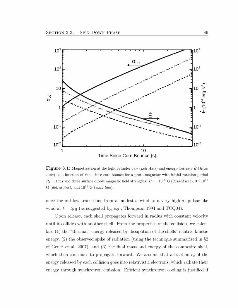
Section 3.3. Spin-Down Phase 89
1 10Time Since Core Bounce (s)
10-2
10-1
1
10
102
103σ L
C
σLC
E.
10-2
10-1
1
10
102
103
E (
1051
erg
s-1)
.
Figure 3.1: Magnetization at the light cylinder σLC (Left Axis) and energy-loss rate E (Right
Axis) as a function of time since core bounce for a proto-magnetar with initial rotation period
P0 = 1 ms and three surface dipole magnetic field strengths: B0 = 1015 G (dashed line), 3×10¹⁵
G (dotted line), and 1016 G (solid line).
once the outflow transitions from a modest-σ wind to a very high-σ, pulsar-like
wind at t = tKH (as suggested by, e.g., Thompson 1994 and TCQ04).
Upon release, each shell propagates forward in radius with constant velocity
until it collides with another shell. From the properties of the collision, we calcu-
late (1) the “thermal” energy released by dissipation of the shells’ relative kinetic
energy, (2) the observed spike of radiation (using the technique summarized in §2
of Genet et al. 2007), and (3) the final mass and energy of the composite shell,
which then continues to propagate forward. We assume that a fraction εe of the
energy released by each collision goes into relativistic electrons, which radiate their
energy through synchrotron emission. Efficient synchrotron cooling is justified if
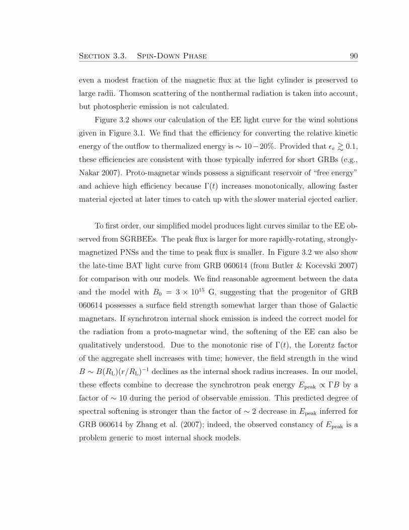
Section 3.3. Spin-Down Phase 90
even a modest fraction of the magnetic flux at the light cylinder is preserved to
large radii. Thomson scattering of the nonthermal radiation is taken into account,
but photospheric emission is not calculated.
Figure 3.2 shows our calculation of the EE light curve for the wind solutions
given in Figure 3.1. We find that the efficiency for converting the relative kinetic
energy of the outflow to thermalized energy is ∼ 10−20%. Provided that εe & 0.1,
these efficiencies are consistent with those typically inferred for short GRBs (e.g.,
Nakar 2007). Proto-magnetar winds possess a significant reservoir of “free energy”
and achieve high efficiency because Γ(t) increases monotonically, allowing faster
material ejected at later times to catch up with the slower material ejected earlier.
To first order, our simplified model produces light curves similar to the EE ob-
served from SGRBEEs. The peak flux is larger for more rapidly-rotating, strongly-
magnetized PNSs and the time to peak flux is smaller. In Figure 3.2 we also show
the late-time BAT light curve from GRB 060614 (from Butler & Kocevski 2007)
for comparison with our models. We find reasonable agreement between the data
and the model with B0 = 3 × 10¹⁵ G, suggesting that the progenitor of GRB
060614 possesses a surface field strength somewhat larger than those of Galactic
magnetars. If synchrotron internal shock emission is indeed the correct model for
the radiation from a proto-magnetar wind, the softening of the EE can also be
qualitatively understood. Due to the monotonic rise of Γ(t), the Lorentz factor
of the aggregate shell increases with time; however, the field strength in the wind
B ∼ B(RL)(r/RL)−1 declines as the internal shock radius increases. In our model,
these effects combine to decrease the synchrotron peak energy Epeak ∝ ΓB by a
factor of ∼ 10 during the period of observable emission. This predicted degree of
spectral softening is stronger than the factor of ∼ 2 decrease in Epeak inferred for
GRB 060614 by Zhang et al. (2007); indeed, the observed constancy of Epeak is a
problem generic to most internal shock models.
Section 3.3. Spin-Down Phase 91
10 100Observer Time (s)
0.0
0.2
0.4
0.6
0.8
1.0
1.2
1.4
Bol
omet
ric L
umin
osity
(10
49 e
rg s
-1)
Figure 3.2: Luminosity of internal shock emission from the proto-magnetar winds in Figure
3.1; electron acceleration efficiency εe = 0.5 is assumed. Note the lack of emission at early times
because the outflow is non-relativistic. The gradual onset of the emission once σLC > 10 is due to
the large Thomson optical depth, which decreases as the outflow expands. The late-time decline
in emission is the onset of curvature emission from the last shock, produced by the shell released
at tKH = 40 s. The late-time BAT light curve from GRB 060614, shown with a light solid line
and scaled to the physical isotropic luminosity, is reproduced in a time-averaged sense by the
B0 = 3× 10¹⁵ G model.
Section 3.4. Discussion 92
3.4 Discussion
Short GRBs with extended emission challenge the paradigm that short GRBs
result exclusively from COMs. The central engine in these systems may instead
be a newly-formed magnetar. The timeline of our model is summarized as follows:
• AIC or WD-WD merger produces a proto-magnetar and a disk of mass ∼
0.1M¯ (t ∼ tdyn ∼ 100 ms)
• Disk accretes onto the proto-magnetar, generating the prompt emission spike
(t ∼ tvisc ∼ 0.1− 1 s; see eq. [3.1])
• Free proto-magnetar wind transitions from non-relativistic to ultra-relativistic
(t ∼ 3− 10 s; see Fig. 3.1)
• Proto-magnetar spins down, generating X-ray emission on observed longer
timescale (t ∼ 10− 100 s; see Fig. 3.2)
A model similar to the one described here was proposed by Gao & Fan (2006); in
their model, late-time flares from short GRBs are powered by dipole spin-down of a
super-massive, transiently-stable magnetar formed by a NS-NS merger. However,
current evidence suggests that SGRBEEs form a distinct population with only
modest offsets from their host galaxies (Troja et al. 2007). If transiently-stable
magnetars from NS-NS mergers indeed produce most SGRBEEs, an equal number
would be expected with large offsets.
A more promising channel of isolated magnetar birth may be the AIC of a
WD or the merger and collapse of a WD-WD binary. The rate of these events
is difficult to constrain directly because the Ni mass synthesized in a PNS wind
is less than ∼ 10−3M¯ (Chapter 4) and is therefore unlikely to produce a bright
optical transient. There is, however, indirect evidence that isolated magnetar
birth occurs in nature. The rapidly-rotating, highly magnetic WD RE J0317-
853 has a mass M = 1.35M¯ and was likely produced from a WD-WD merger;
if RE J0317-853’s progenitor binary had been slightly more massive, it would
probably have collapsed to a rapidly-rotating magnetar (King et al. 2001). Isolated
Section 3.4. Discussion 93
NS birth via AIC is also one of the only Galactic r-process sites consistent with
current observations of elemental abundances in metal-poor halo stars (Qian &
Wasserburg 2007). Although unmagnetized PNS winds fail to produce successful
r-process (T01), proto-magnetar winds may be sufficiently neutron-rich to produce
∼ 0.1M¯ in r-process elements (D07; Chapter 4). For AIC or WD-WD mergers
to produce the entire Galactic r-process yield requires a rate ∼ 10−5 − 10−6 yr−1,
comparable to the observed local short GRB rate (Nakar 2007). Finally, Levan
et al. (2006) argue that the correlation found by Tanvir et al. (2005) between a
subset of short GRBs and local large-scale structure is evidence for a channel of
isolated magnetar birth, if these bursts are produced by SGR-like flares.
A theory for SGRBEEs must explain the large burst-to-burst variation in the
ratio of the flux/fluence of the prompt and EE components (NB06). The angular
momentum of AIC and WD-WD mergers may vary between events, resulting in
a wide distribution in both the properties of the accretion disk formed (which
influences the prompt emission) and the rotation rate of the proto-magnetar (which
determines the EE). Event-to-event variability may also result from the viewing
angle θobs of the observer with respect to the rotation axis. The spin-down power of
the magnetar varies as E ∝ sin2(θobs) for σLC À 1; hence, the light curves in Figure
3.2 remain reasonably accurate for moderately large θobs, but a viewer looking down
the rotation axis (θobs ∼ 0) may observe little or no EE. Conversely, equatorial
viewers would observe EE but no prompt spike; therefore, this model predicts a
class of long-duration X-ray flashes (XRFs) not associated with very massive star
formation or accompanied by a SN. Such an event may have already been observed.
GRB 060428b is an XRF with a light curve similar to the EE from GRB 060614
which was localized inside a red galaxy at redshift z = 0.347. Assuming this galaxy
is the host, GRB 060428b released an isotropic energy ∼ 2×1050 ergs, comparable
to EE of GRB 060614, and showed no SN component at one month down to an
optical brightness ∼ 20 times fainter than SN1998bw (Perley et al., in prep).
Because the EE flow is symmetric in azimuth, equatorial viewers should not
observe a classic jet-break (although a more shallow break is possible; Thompson
2005). Furthermore, although only Γ & 10 material contributes to the EE in
Section 3.4. Discussion 94
Figure 3.2, the magnetar releases ∼ 1052 ergs in earlier, mildly relativistic material
(Γ ∼ 1 − 10; see Fig. 3.1) that is hoop-stress collimated along the PNS rotation
axis. This material may become visible as a radio transient as it slows down and
becomes non-relativistic on a timescale of months to years. If AIC or WD-WD
mergers indeed produce SGRBEEs, these events should be bound to both early
and late type galaxies; indeed, the well-known SGRBEEs 050709 and 050724 were
localized to a star forming galaxy and an elliptical galaxy, respectively (Villasenor
et al. 2005; Berger et al. 2005). Unlike COMs, magnetar birth from AIC or WD-
WD mergers should not produce strong gravitational wave emission, and because
the magnetar will not collapse to a BH, its magnetic energy could power late-time
X-ray flares.
Although we have concentrated on spin-down-powered EE, isolated NS birth
may produce the EE of SGRBEEs in other ways. Specifically, the accretion disk
produced by a WD-WD merger prior to collapse (e.g., Yoon et al. 2007) may
accrete onto the NS at later times, powering a bipolar outflow similar to that
produced during the prompt accretion episode; in this case, the delay until EE
reflects the accretion timescale at the WD radius (∼ 109 cm), which D07 estimate
is tvisc ∼ 100 s for α ∼ 0.1. Late-time accretion and spin-down powered EE can be
distinguished based on the presence or absence, respectively, of a jet break and the
observed ratio of SGRBEEs to off-axis, purely-EE XRFs. Assuming that jets from
the prompt and delayed accretion episodes are similarly collimated, SGRBEEs
with accretion-powered EE should not be visible off-axis; by contrast, if the EE is
powered by magnetar spin-down at least as many off-axis XRFs are expected as
standard SGRBEEs.
Finally, it is important to distinguish the observable signature of a magnetar
produced by an AIC, WD-WD merger, or NS-NS merger from that produced by
the core collapse of a massive star, which may instead produce a traditional long-
duration GRB (e.g., Chapter 2). The magnetic fields and rotation rates of the
magnetars produced via these channels may differ, which would modify E and
σ of the wind (Fig. 3.1) and hence its observable properties. Although isolated
magnetar spin-down may be comparatively simple because the proto-magnetar
Section 3.4. Discussion 95
wind expands relatively freely into space, a free magnetar wind is nearly isotropic
and so its emission is relatively weak and difficult to detect. By contrast, the wind
from a magnetar produced via core collapse is collimated into a bipolar jet by
the overlying stellar mantle (Uzdensky & MacFadyen 2006; Komissarov & Barkov
2007; Bucciantini et al. 2007) and the observed emission can be much brighter due
to the jet’s modest opening solid angle.
Acknowledgements
We thank J. Bloom, N. Bucciantini, N. Butler, D. Perley, A. Spitkovsky, and
E. Troja for helpful discussions and information. EQ and BDM were supported
by the David and Lucile Packard Foundation and a NASA GSRP Fellowship.
96
Chapter 4
On the Conditions for
Neutron-Rich Gamma-Ray Burst
Outflows
B. D. Metzger, T. A. Thompson, E. Quataert, ApJ, 676:1130-1150, 2008 April 1.1
Abstract
We calculate the structure and neutron content of neutrino-heated magneto-
hydrodynamic winds driven from the surface of newly-formed magnetars (“proto-
magnetars”) and from the midplane of hyper-accreting disks, two of the possi-
ble central engines for gamma-ray bursts (GRBs) and hyper-energetic supernovae
(SNe). Both the surface of proto-magnetars and the midplane of neutrino-cooled
accretion flows (NDAFs) are electron degenerate and neutron-rich (neutron-to-
proton ratio n/p À 1). If this substantial free neutron excess is preserved to
large radii in ultra-relativistic outflows, several important observational conse-
quences may result. Weak interaction processes, however, can drive n/p to ∼ 1
in the nondegenerate regions that obtain just above the surfaces of NDAFs and
proto-magnetars. Our calculations show that mildly relativistic (Lorentz factor
1Copyright 2008. The American Astronomical Society. All rights reserved.
Section 4.1. Introduction 97
Γ . 10) neutron-rich outflows from NDAFs are possible in the presence of a strong
poloidal magnetic field. However, neutron-rich winds possess a minimum mass-
loss rate that likely precludes simultaneously neutron-rich and ultra-relativistic
(Γ & 100) NDAF winds accompanying a substantial accretion power. In con-
trast, proto-magnetars are capable of producing neutron-rich long-duration GRB
outflows ∼ 10−30 seconds following core bounce for sub-millisecond rotation peri-
ods; such outflows would, however, accompany only extremely energetic events, in
which the GRB + SN energy budget exceeds ∼ 4× 1052 ergs. Neutron-rich highly
relativistic outflows may also be produced during some short-duration GRBs by
geometrically thick accretion disks formed from compact object mergers. The im-
plications for r-process nucleosynthesis, optical transients due to non-relativistic
neutron-rich winds, and Nickel production in proto-magnetar and NDAF winds
are also briefly discussed.
4.1 Introduction
The rapid variability and large energies that characterize cosmological gamma-
ray bursts (GRBs) strongly implicate stellar-mass compact objects as their cen-
tral engines. Indeed, the association of several long-duration GRBs (LGRBs)
with Type Ibc supernovae (SNe) suggests that LGRBs result from relativistic out-
flow accompanying rapid accretion onto a newly-formed black hole (a “collapsar”;
Woosley 1993; MacFadyen & Woosley 1999; Woosley & Bloom 2006) or the spin-
down of a newly-formed magnetar (e.g., Usov 1992; Thompson 1994; Blackman
& Yi 1998; Wheeler et al. 2000; Thompson, Chang, & Quataert 2004, hereafter
TCQ04). Short-duration GRBs may result from black hole accretion-powered out-
flows following the tidal disruption and coalescence of compact binaries (Paczynski
1986, 1991; Eichler et al. 1989; Narayan et al. 1992; Ruffert et al. 1997; Janka et
al. 1999).
A unique property of both the surface of a newly-formed neutron star (a
“proto-neutron star” or PNS; Burrows & Lattimer 1986) and in some cases the
midplane of hyper-accreting disks is a significant excess of free neutrons (elec-
Section 4.1. Introduction 98
tron fraction Ye ¿ 0.5), resulting from β-equilibrium under electron degeneracy
(Pruet et al. 2003; Beloborodov 2003a, hereafter B03a).2 While degeneracy at
the neutrinosphere of PNS is assured, hyper-accreting disks are viscously heated
and only possess a neutron excess in places where they are sufficiently dense and
efficiently neutrino-cooled. If present at all, these neutrino-dominated accretion
flows (or NDAFs) are thus geometrically-thin and confined to small radii in the
disk (Popham et al. 1999). Recent neutrino-cooled α-disk calculations show that
an NDAF only forms outside the last stable orbit for steady-state mass accretion
above a critical “ignition” rate, given by
Mign ≈ 0.07(0.02)M4/33 α
5/30.1M¯ s
−1 (4.1)
for black hole mass M = 3M3M¯ and spin a = 0(0.95), where α = 0.1α0.1 is
the disk viscosity parameter (Chen & Beloborodov 2007, hereafter CB07). Disk
mass accretion rates (MD) greater than Mign, and thus neutron-rich NDAFs, are
plausible in both collapsar and binary merger scenarios (e.g., Popham et al. 1999).
For lower accretion rates or larger radii than characterize NDAFs, cooling
is inefficient and the accretion is geometrically-thick and quasi-virial, forming an
advection dominated accretion flow (Narayan & Yi 1994; Narayan et al. 2001).
Although NDAFs must come into β-equilibrium before accreting (B03a), this is
not necessarily the case for thick disks; the neutron content of a thick disk may
therefore depend on the matter that feeds it. We discuss the likely neutron content
of thick disk winds more in §4.5.5 and §4.6.3.
If the neutron excess that characterizes proto-magnetars and NDAFs can be
preserved to large radii in the outflows that they power (where Ye obtains its
asymptotic value Y ae ; see Table 4.2 for definitions of commonly used variables),
observable consequences may result. The dynamics of the GRB jet may be al-
tered by the presence of a dominant neutron component (Derishev, Kocharovsky,
and Kocharovsky 1999), which at proton-neutron decoupling could result in the
emission of multi-GeV photons and neutrinos (Bahcall & Meszaros 2000; Meszaros
2In this paper we define a neutron excess as a neutron-to-proton ratio n/p = (1−Ye)/Ye > 1,where we assume free nucleons and Ye is the proton-to-baryon ratio or “electron fraction.”
Section 4.1. Introduction 99
& Rees 2000; Razzaque & Meszaros 2006a) and cause a significant reheating of
the outflow (Rossi et al. 2006). Furthermore, a large neutron-to-proton ratio n/p
may reduce the fireball’s asymptotic baryon contamination (Fuller et al. 2000;
Vlahakis et al. 2003), contribute an additional component to the GRB light curve
(Pruet & Dalal 2002; Bulik, Sikera, & Moderski 2002; Fan & Wei 2004; Fan et
al. 2005; Dermer & Atoyan 2006) and a unique beta-decay signature (Razzaque
& Meszaros 2006b), alter the subsequent afterglow emission (Beloborodov 2003b),
and affect the fireball’s nucleosynthetic yield (Lemoine 2002; Pruet et al. 2002;
B03a). Although not all of these consequences strictly require a neutron excess,
most are far more conspicuous when n/pÀ 1, partly because only excess neutrons
will ultimately remain free if α-particle formation is efficient (e.g., Lemoine 2002).
Identification or strong upper limits on any of these effects would teach us much
about the composition of GRB outflows.
In this paper we examine the processes that shape the neutron content of
outflows from GRB progenitors, motivated by the promise that the distinctive
neutron-rich GRB signature holds as a tool for constraining the elusive central
engine, whose properties are masked by the otherwise rather generic dynamical
evolution of the outflow (e.g., the “fireball” model; Rees & Meszaros 1992). In
particular, we focus on NDAFs and proto-magnetars rather than thick accretion
disks, not because these models are necessarily favored to produce GRBs, but
rather because for neutron-rich central engines an asymptotically neutron-rich out-
flow is plausible a priori. The goal of our analysis is to determine the conditions
under which and degree to which these neutron-rich central engines can produce
equally neutron-rich outflows.
Determining the asymptotic neutron content of winds driven from the neutron-
rich base of PNSs and NDAFs is nontrivial because the neutron fraction will evolve
due to weak interactions under the comparatively nondegenerate conditions that
characterize scales immediately larger than that of the central engine. In §4.1.1 we
discuss the relevant processes that may “deneutronize” the outflow, driving n/p
back to ∼ 1. Indeed, in §4.2 we show that thermally-driven outflows from PNSs
and NDAFs are generally deneutronized by, if nothing else, electron neutrino ab-
Section 4.1. Introduction 100
sorption. Although thermally-driven winds of this kind possess little or no neutron
excess, they also cannot produce GRBs because they do not reach ultra-relativistic
speeds (Lorentz factor ΓÀ 1). Winds driven directly from the surface of PNSs or
the midplane of NDAFs require an energetically-dominant Poynting flux to reach
large Γ because of the significant mass-loss driven by viscous and neutrino heating
(e.g., Levinson & Eichler 1993); this requires rapid rotation and a strong magnetic
field. If, through such enhanced magnetic acceleration matter is advected from
the PNS surface or the NDAF midplane sufficiently rapidly to avoid deneutron-
ization, the outflow will retain the large neutron-to-proton ratio that characterizes
its degenerate base. The magnetocentrifugal acceleration required to maintain low
Ye (high n/p), however, also enhances the wind’s mass-loss rate over its purely
thermally-driven value (TCQ04). This raises the question of whether simulta-
neously neutron-rich and ultra-relativistic outflows are possible under physically
realizable conditions.
To address these issues quantitatively we have calculated the neutron content
of magnetically-driven winds from proto-magnetars and hyper-accreting NDAF
disks by solving the equations of one-dimensional neutrino-heated magnetohydro-
dynamics (MHD). We have studied in detail the effects of magnetic fields and
rotation on PNS winds in a previous work, assuming a constant Ye (Chapter 2).
In §4.4 we include the evolution of Ye in these calculations in order to determine
the asymptotic electron fraction Y ae from proto-magnetar outflows. In §4.5 we
adapt our calculations to the NDAF context by following outflow from the ac-
cretion disk midplane for several flux tube angles, employing the α-disk NDAF
models of CB07 as boundary conditions. We present a summary of our results in
§4.6, including a discussion of the prospect for neutron-rich outflows from central
engines of both long and short-duration GRBs. Our analysis and conclusions can
be summarized in the broadest terms as follows: the conditions for n/p À 1 are
simultaneously the conditions for short advection timescale, large mass-loss rate,
and low asymptotic Lorentz factor. Thus only under very restrictive conditions do
both n/p À 1 and high Γ obtain. The most promising possibilities appear to be
outflows from sub-millisecond proto-magnetars and from geometrically thick disks
Section 4.1. Introduction 101
with MD . Mign (see Table 4.1).
4.1.1 Deneutronizing Processes
Despite the presence of neutron-rich material at the base of NDAF and PNS
outflows, this neutron excess may not be preserved. Because conditions above
the PNS surface and the accretion disk midplane are typically nondegenerate,
equilibrium between the pair-capture reactions
e− + p→ n+ νe, (4.2)
e+ + n→ p+ νe (4.3)
favor Ye > 0.5 in the potentially pair-rich atmosphere through which the wind must
accelerate. Furthermore, in the presence of an electron neutrino(antineutrino)
energy density uνe(uνe) the inverse, neutrino absorption reactions
νe + n→ e− + p, (4.4)
νe + p→ e+ + n, (4.5)
which dominate pair-captures abruptly above the launching surface of the outflow,
drive the system toward an asymptotic electron fraction given by
Y νe ≡
(
1 +uνeuνe
〈ενe〉 − 2∆ + 1.2∆2/〈ενe〉
〈ενe〉+ 2∆ + 1.2∆2/〈ενe〉
)−1
, (4.6)
where ∆ = 1.293 MeV is the neutron-proton mass difference, 〈ενe〉(〈ενe〉) is the
mean electron neutrino(antineutrino) energy (Qian et al. 1993; Qian & Woosley
1996, hereafter QW96), and the superscript ν denotes that the electron fraction
given by equation (4.6) is set solely by the properties of the local neutrino radiation
field.
Equation (4.6) shows that when the electron neutrino and antineutrino fluxes
are comparable and have a similar spectrum, as is generically the case for NDAFs
and PNSs during the latter’s Kelvin-Helmholtz cooling phase (Burrows & Lat-
timer 1986), equilibrium between neutrino absorptions also favors a comparatively
Section 4.1. Introduction 102
neutron-poor state (Ye ∼ 0.5).3 Such a deneutronizing luminosity of neutrinos
must be present, self-consistently, for matter to cool to the dense, degenerate con-
ditions required for low Ye in the first place. The total neutrino luminosity from a
neutron-rich NDAF, for instance, must exceed
Lν,ign ≡ ηMignc2 ≈ 5× 1051M
4/33 α
5/30.1 ergs s−1, (4.7)
where η ≈ 0.04(0.15) for a = 0(0.95) (CB07) and we have used equation (4.1) for
Mign. Similarly, detailed numerical calculations show that a cooling PNS’s electron
neutrino/antineutrino luminosity is approximately given by
Lν ≈ 1052(t/ 1 s)−1 ergs s−1 (4.8)
from a time t ≈ 1 s after core bounce until the end of the Kelvin-Helmholtz epoch
at t = τKH ∼ 10− 100 s (see, e.g., Pons et al. 1999, Fig. 14).
To contrast the large neutron fraction in an NDAF’s midplane with the much
lower value favored in equilibrium with the NDAF’s neutrino flux, Figure 4.1 shows
the midplane electron fraction Y De (dashed line) and the equilibrium electron
fraction set by neutrino absorption Y νe (solid line) as a function of disk cylindrical
radius R0 (in units of gravitational radii Rg ≡ GM/c2) for a steady-state NDAF
solution taken from CB07 with α = 0.03, M = 3M¯, a = 0, and MD = 0.2M¯
s−1. The local neutrino energy densities (uνe ,uνe) and mean energies (〈ενe〉,〈ενe〉)
used to calculate Y νe from equation (4.6) were obtained by integrating the total
flux incident on a given position just above the disk midplane at radius R0, where
Y ae for an outflow launched near R0 is set. The disk neutrino emission is assumed
to originate from axisymmetric annuli of negligible vertical height with a radial
structure taken from CB07’s one-dimensional, height-integrated calculations. We
assume that all relevant lines of site are optically thin in calculating Y νe ; this is a
good approximation because the vertical neutrino optical depth through the disk
3During deleptonization, efficiently neutrino-cooled central engines release slightly more νe’sthan νe’s; in addition, the νe and νe spectra (and thus mean energies) also differ slightly due tothe difference between the mean e− and e+ energies, the e− and e+ capture cross sections, and,in the neutrino optically thick case, the νe and νe neutrinosphere temperatures and geometries.Although Y ν
e . 0.5 is possible in some cases, these relatively modest effects are unlikely to yieldY νe ¿ 0.5.
Section 4.2. Thermally-Driven Winds 103
is . 1 at all radii and because the disc scale height increases more rapidly than
∝ R0 so that the outer disk’s atmosphere has an unobstructed view of the interior
flow. Differential gravitational redshifts between emission and absorption radii are
taken into account, although geodesic bending is ignored.
Figure 4.1 shows that the disk midplane is very neutron-rich for R0 . 30 −
100Rg (the NDAF portion of the disk), reaching a neutron-to-proton ratio as large
as ∼ 30 at small radii. However, Figure 4.1 also shows that Y νe ∼ 0.5 at all radii, so
that if the outflow comes into equilibrium with the disk’s neutrino luminosity it will
be driven back to a relatively neutron-poor state (n/p ∼ 1). Also note that Y νe >
0.485 at all radii, allowing possible 56Ni synthesis in a disk wind, again should the
nucleons come into equilibrium with the neutrino flux (Pruet et al. 2004).4 Since
the outer disk is radiatively-inefficient and therefore particularly prone to large
mass outflows (Blandford & Begelman 1999), disk wind-aided stellar explosions
provide one way to produce optically luminous SNe in collapsar models for LGRBs
(MacFadyen & Woosley 1999), where Ni masses up to ∼ 0.5M¯ have been inferred
(e.g., GRB980425/SN1998bw; Iwamoto et al. 1998; Woosley, Eastman, & Schmidt
1999).
4.2 Thermally-Driven Winds
In spite of nondegenerate pair captures and neutrino absorptions (eqs. [4.2]–
[4.5]), the high neutron fraction in NDAFs and proto-magnetar outflows will be
preserved if deneutronization proceeds slower than a fluid element’s advection from
the surface. In evaluating this possibility in the case of NDAFs, previous investi-
gations have assumed that the disk is turbulent and that the relevant outflow rate
is of the order of the turnover frequency of a typical turbulent eddy (∼ ΩK, the
4Although we find that Y νe > 0.485 at all disk radii using mean neutrino energies from
CB07’s height-integrated disk calculations, precisely whether Y νe > 0.485 or Y ν
e < 0.485 isdifficult to determine with confidence because the neutrino spectra are sensitive to the disk’svertical temperature profile, which is theoretically uncertain, and to neutrino transport if thedisk midplane is neutrino optically thick (Sawyer 2003). If viscous heating is important in thewind, additional entropy deposition may drive Y a
e & 0.485, allowing 56Ni production even ifY νe < 0.485.
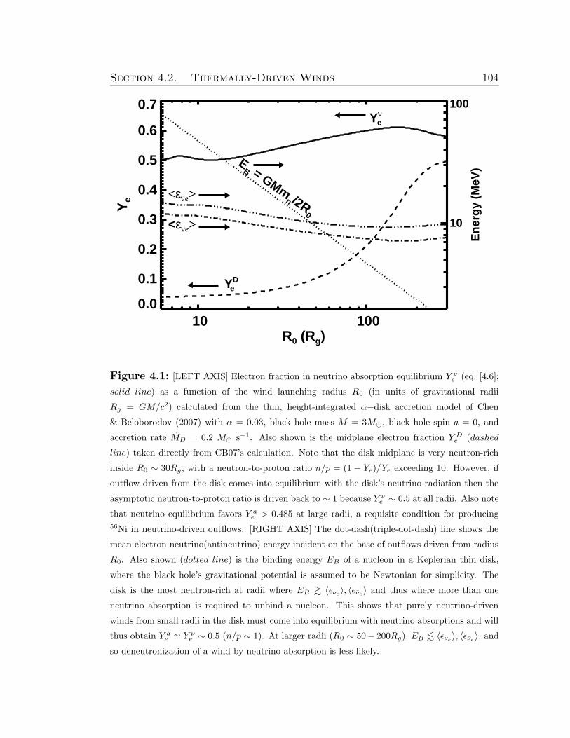
Section 4.2. Thermally-Driven Winds 104
10 100R0 (Rg)
0.0
0.1
0.2
0.3
0.4
0.5
0.6
0.7Y
e
10
100
En
erg
y (M
eV)E
B = GMmn /2R
0
Yνe
YDe
<ενe>
<ενe>_
Figure 4.1: [LEFT AXIS] Electron fraction in neutrino absorption equilibrium Y νe (eq. [4.6];
solid line) as a function of the wind launching radius R0 (in units of gravitational radii
Rg = GM/c2) calculated from the thin, height-integrated α−disk accretion model of Chen
& Beloborodov (2007) with α = 0.03, black hole mass M = 3M¯, black hole spin a = 0, and
accretion rate MD = 0.2 M¯ s−1. Also shown is the midplane electron fraction Y De (dashed
line) taken directly from CB07’s calculation. Note that the disk midplane is very neutron-rich
inside R0 ∼ 30Rg, with a neutron-to-proton ratio n/p = (1 − Ye)/Ye exceeding 10. However, if
outflow driven from the disk comes into equilibrium with the disk’s neutrino radiation then the
asymptotic neutron-to-proton ratio is driven back to ∼ 1 because Y νe ∼ 0.5 at all radii. Also note
that neutrino equilibrium favors Y ae > 0.485 at large radii, a requisite condition for producing
56Ni in neutrino-driven outflows. [RIGHT AXIS] The dot-dash(triple-dot-dash) line shows the
mean electron neutrino(antineutrino) energy incident on the base of outflows driven from radius
R0. Also shown (dotted line) is the binding energy EB of a nucleon in a Keplerian thin disk,
where the black hole’s gravitational potential is assumed to be Newtonian for simplicity. The
disk is the most neutron-rich at radii where EB & 〈ενe〉, 〈ενe
〉 and thus where more than one
neutrino absorption is required to unbind a nucleon. This shows that purely neutrino-driven
winds from small radii in the disk must come into equilibrium with neutrino absorptions and will
thus obtain Y ae ' Y ν
e ∼ 0.5 (n/p ∼ 1). At larger radii (R0 ∼ 50− 200Rg), EB . 〈ενe〉, 〈ενe
〉, and
so deneutronization of a wind by neutrino absorption is less likely.
Section 4.2. Thermally-Driven Winds 105
Keplerian rotation rate), concluding that low Ye is preserved under most conditions
appropriate to hyper-accreting disks (Pruet et al. 2003; B03a). Specifically, Pruet
et al. (2003) argue that because NDAFs are generally dense, degenerate, and gas
pressure-dominated, if a fluid element is carried out of the midplane adiabatically
in an eddy turnover time, pair creation is somewhat suppressed and low Ye is pre-
served (i.e., Y ae ≈ Y D
e obtains). B03a also compares ΩK to the neutrino absorption
rates (eqs. [4.4]−[4.5]), reaching a similar conclusion to Pruet et al. (2003) except
for very high disk neutrino luminosities (Lν & 1053 erg s−1), corresponding to
MD & 1M¯ s−1. This leaves a wide range of astrophysically plausible accretion
rates (Mign . MD . 1M¯ s−1) for which outflow, if it escapes the disk in an eddy
turnover time, would be asymptotically neutron-rich.
Several arguments can, however, be raised against the conclusion that low Ye
is preserved in NDAF outflows. Although some degree of turbulence and turbulent
mixing must accompany the accretion torque (e.g., via the MRI; Balbus & Hawley
1998), its scale and efficiency are unclear.5 Even if present, large-scale turbulence
is not likely to drive outflow from a thin disk; thus, an eddy turnover time is not
the relevant timescale to compare to the weak interaction rates. Outflow from
the surface of a thin accretion disk must be heated, passing through a sonic point
as it accelerates out of the black hole’s potential. Thus, the advection time of a
self-consistent, viscous or neutrino-heated wind sets the residence time for a fluid
element in regions of potential deneutronization. This timescale is generally much
longer than Ω−1K .
Indeed, the neutrino-driven PNS winds that accompany the Kelvin-Helmholtz
cooling of slowly rotating, non-magnetized PNSs generically come into equilibrium
with the neutrino absorption rates, obtaining Y ae = Y ν
e (QW96; Thompson et
al. 2001, hereafter T01). To see that the neutron fraction of a purely neutrino-
driven NDAF wind must also come into equilibrium with the neutrino rates we
adapt an argument first presented by QW96 in the PNS context. First, note that a
5NDAFs cool efficiently and are not unstable to radial convection, except perhaps at smallradii in the case of neutrino optically thick accretion (Lee et al. 2005); it is also not clear thatNDAFs are vertically-convective (Hirose, Krolik, & Stone 2006), as this depends on the unknownvertical viscous dissipation profile (see the discussion in Blaes 2007).
Section 4.2. Thermally-Driven Winds 106
typical nucleon with massmn launched in a wind from radius R0 of a thin Keplerian
disk requires an energy EB ' GMmn/2R0 ≈ 80(R0/6Rg)−1 MeV to escape the
black hole’s gravitational potential, where we have assumed Newtonian gravity for
simplicity. In addition to Y De and Y ν
e , in Figure 4.1 we show for comparison EB
and the mean electron neutrino and antineutrino energies used to calculate Y νe .
The mean neutrino energies vary only weakly with radius because the neutrino
flux released from an NDAF’s inner disk is relatively hot (Popham et al. 1999;
CB07) and dominates the neutrino heating at all outflow radii (relative to the
neutrino emission from larger radii in the disk). By balancing viscous heating and
optically thin neutrino cooling at the radius Rp ∼ 1 − 10Rg where most of the
disk’s emission originates, we find that an NDAF’s mean neutrino energy incident
on any disk radius is approximately given by
〈εν〉 ≈ 5.1TD ≈ 18α1/50.1M
−1/53 (Rp/6Rg)
−3/10 MeV, (4.9)
where TD is the disk’s midplane temperature at Rp. Equation (4.9), which agrees
well with our calculation of 〈εν〉 in Figure 4.1, is valid so long as the inner disk
is optically thin to neutrinos (τν . 1), which remains true for accretion rates
below ≈ 0.7(0.05)α0.1M¯ s−1 for electron neutrinos and ≈ 2.0(0.14)α0.1M¯ s
−1 for
electron antineutrinos for a = 0(0.95) and M = 3M¯ (CB07). For larger MD
the disk is opaque to neutrinos (τνe , τνe & 1) and the mean neutrino energy is
approximately given by its Fermi-Dirac blackbody value
〈εν〉 ≈ 3.2Tν ≈ 16M−1/23 M
1/4D,0.1(Rp/6Rg)
−1/2MeV, (4.10)
where MD = 0.1MD,0.1M¯ s−1 and Tν is the temperature at the disk’s neutri-
nosphere.
Despite the relatively high mean neutrino energies shown in Figure 4.1 and
implied by equations (4.9)− (4.10), 〈εν〉 is still much less than EB(∼ Rp) because
NDAFs are efficiently neutrino-cooled. Thus, each nucleon in a thermally-driven
outflow originating from an inner NDAF must absorb several neutrinos in the
process of being unbound from the black hole’s potential. Through these multiple
absorptions the wind’s electron fraction is unavoidably brought into equilibrium
Section 4.2. Thermally-Driven Winds 107
with the neutrino flux at Y νe (QW96), a consequence of the fact that neutrino
absorptions (eqs. [4.4]−[4.5]) both dominate the wind heating and determine Y ae '
Y νe .
This conclusion may hold even for winds driven from near the NDAF’s rela-
tively loosely-bound outer edge. NDAFs only exist interior to an “ignition” radius
Rign, which we estimate as the location at which optically thin cooling by nonde-
generate pair capture on free nuclei (eqs. [4.2]−[4.3]) balances viscous heating for
a thick disk:6
Rign ≈ 10M6/5D,0.1M
−8/53 α−20.1Rg. (4.11)
For the disk parameters associated with the solution in Figure 4.1 (α = 0.03,M =
3M¯, MD = 0.2M¯ s−1 À Mign), equation (4.11) gives Rign ≈ 100Rg, correspond-
ing to the radius interior to which the disk possesses a significant neutron excess
(Y De ¿ 0.5). By requiring that Rign exceed the radius of the innermost stable
circular orbit, Risco ' 6(1)Rg for black hole spin a = 0(0.95), one recovers the
numerically-determined value for Mign given in equation (4.1) to reasonable accu-
racy.
Using equations (4.9) and (4.10), the ratio of the binding energy at Rign to
the mean neutrino energy from the inner disk is approximately given by
EB(Rign)
〈εν〉∼ 3M
−6/5D,0.1M
9/53 α
9/50.1
(
Rp
6Rg
)3/10
: τν . 1
∼ 3M−29/20D,0.1 M
21/103 α2
0.1
(
Rp
6Rg
)1/2
: τν & 1
(4.12)
Equation (4.12) shows that EB(Rign) & 〈εν〉 for α & 0.1 and for most physical
values of MD; thus, winds thermally-driven from even R0 ∼ Rign would have
Y ae ≈ Y ν
e ∼ 0.5. Although equation (4.12) implies that winds driven from the outer
portions of high-MD, low-α NDAFs may remain neutron-rich, the astrophysical
6Equation (4.11) overestimates Rign for large Rign (i.e., large MD and low α) because coolingvia electron capture requires a threshold energy ∆ − mec
2 ∼ 1 MeV that exceeds the disktemperature at large radii. Furthermore, NSE favors composite nuclei for R0 > Rα ∼ 100Rg;nuclear disintegration is a significant heat source around R0 ∼ Rα and we have overestimatedcooling for R0 > Rα because pair capture rates are lower on composite nuclei.
Section 4.3. Magnetically-Driven Winds 108
situations most likely to result in extended disks, collapsars and He core-black
hole mergers (Fryer & Woosley 1998), are also likely to have lower values of MD.
Furthermore, NDAFs become unstable to self-gravity (Toomre Q < 1) at Rign for
MD & 2α10/70.1 M
3/113 M¯ s−1, comparable to the accretion rates for which EB(Rign) <
〈εν〉. The dynamics at these radii is not well understood so it is difficult to draw
definitive conclusions concerning the neutron content of outflows launched from
large radii in high-MD, low-α disks.
In addition to neutrino heating, viscous heating may thermally drive outflows
from the surface of NDAFs. Pruet et al. (2004) have shown, in the context of
a wind driven by viscous heating supplied through a simple α prescription, that
entropy added to the outflow lifts electron degeneracy before the outflow falls out
of β-equilibrium. This drives n/p to a value near unity via nondegenerate pair
captures, even without the aid of neutrino absorption. However, the ability of
viscous heating to generically drive outflows from thin disks is unknown, as this
depends in detail on where energy is deposited, a major uncertainty in current thin
disk theory (Blaes 2007). Recent radiation MHD thin disk simulations suggest
that very little energy dissipation occurs in the disk corona (Turner 2004; Hirose,
Krolik, & Stone 2006; Blaes et al. 2006b; Krolik et al. 2007), where a wind would
most likely be launched. Regardless of potential viscous entropy contributions,
the existence of the neutrino flux discussed in the preceding paragraphs is assured.
We thus conclude that purely thermally-driven winds from the vicinity of compact
objects, even those with a significant surface neutron excess, are unlikely to be
neutron-rich asymptotically.
4.3 Magnetically-Driven Winds
Winds driven directly from the surfaces of NDAFs and PNSs solely by viscous
or neutrino heating are inherently mass-loaded and thus make poor candidates for
producing GRBs. The high energy-to-baryon ratio required of ultra-relativistic
GRB outflows (asymptotic wind Lorentz factor Γ & 10−100; e.g., Lithwick & Sari
2001) can, however, be achieved if rapid rotation and a strong poloidal magnetic
Section 4.3. Magnetically-Driven Winds 109
field supply an energetically dominant Poynting flux. The ratio of Poynting flux
to kinetic energy flux at the light cylinder RL ≡ c/Ω is given by (for σ > 1)
σ ≡B2
4πρc2
∣
∣
∣
∣
RL
, (4.13)
where B is the magnetic field strength, ρ is the rest mass density, Ω is the rotation
rate of the central star or disk, and we have assumed that the outflow is moving
only mildly relativistically at RL. If the magnetic energy is fully converted into
the kinetic energy of bulk motion, either directly or through thermalization and
subsequent thermal or magnetic pressure-driven expansion (e.g., Drenkhahn &
Spruit 2002), then Γ ∼ σ; Poynting-flux dominated GRB outflows therefore require
σ & 10− 100.
In the case of magnetically-driven, high-σ NDAF or PNS winds, matter may
be advected from the wind’s base sufficiently quickly to remain effectively adi-
abatic, with its initial degeneracy never lifted due to insufficient heating. The
pair-capture reactions (eqs. [4.2]−[4.3]) then continue to favor low Ye above the
PNS surface or disk midplane. In the PNS case this ineffective heating becomes
manifest as an exponential drop in the asymptotic wind entropy with increasing Ω,
which occurs for rotation periods P = 2π/Ω . 2−3 ms (see eq. [2.38]) in the pres-
ence of a sufficiently strong surface dipole magnetic field (Bdipν ∼ 1014 − 1015 G);
note that the large fields and rapid rotation required are similar to those required
for proto-magnetars to produce LGRBs in the first place. It is therefore likely that
GRB jets from proto-magnetars or NDAFs are not completely deneutronized by
pair captures.
Even with degeneracy intact and pair production suppressed, to remain neutron-
rich a GRB-producing wind must advect material from its base sufficiently rapidly
to overcome neutrino absorptions. This requires significant magnetocentrifugal
support in the outflow’s inner, hydrostatic atmosphere, where Y ae is set. For the
reasons discussed in §4.2, magnetocentrifugal forces acting on a wind launched from
a radius R must contribute a factor ∼ GMmn/R〈εν〉 À 1 more energy than neu-
trino heating in unbinding the outflow to avoid deneutronization. Inevitably, such
acceleration in the wind’s subsonic region leads to significantly enhanced mass-loss
Section 4.4. Proto-Magnetar Winds 110
(TCQ04; Chapter 2). Thus, the very conditions required to preserve low Ye in a
proto−magnetar or NDAF wind threaten to simultaneously over− pollute the
outflow with baryons, reducing σ and stiflying the outflow′s GRB potential.
In the following sections we address some of these issues by calculating the
neutron content of magnetized proto-magnetar and NDAF winds. In particular,
we consider the conditions under which outflows from proto-magnetars (§4.4) and
NDAFs (§4.5) can remain neutron-rich while simultaneously maintaining suffi-
ciently low mass-loading to remain plausible GRB central engines.
4.4 Proto-Magnetar Winds
4.4.1 Evolution Equations and Numerical Procedure
As in Chapter 2, we calculate the structure of rapidly rotating PNS winds
by solving the equations of one-dimensional neutrino-heated, ideal MHD in the
equatorial plane of the PNS. Using the time-dependent “inhomogeneous” 2N-RK3
scheme described in Brandenburg (2003), we solve for the wind density ρ, temper-
ature T , radial velocity vr, azimuthal magnetic field Bφ, and azimuthal velocity
vφ as a function of radius r according to equations (2.2)-(2.5) and equation (2.9)
in Chapter 2. In this work we extend our previous calculations by simultane-
ously solving for the electron fraction Ye, thus determining the wind’s asymptotic
neutron abundance.
The electron fraction Ye evolves as the wind emerges off the PNS surface due
to weak interactions according to:
d
dtYe = (1− Ye)(λνen→pe− + λe+n→pνe)−
Ye(λνep→ne+ + λe−p→nνe), (4.14)
where d/dt ≡ ∂/∂t+ vr(∂/∂r) and the λ’s are the weak interaction rates; we take
the pair capture rates (eqs. [4.2]–[4.3]) and the neutrino capture rates (eqs. [4.4]–
[4.5]) from B03a (neglecting proton/neutron recoil to good approximation; Strumia
& Vissani 2003). We have included the full effects of electron degeneracy, including
Section 4.4. Proto-Magnetar Winds 111
the outgoing electron and positron blocking factors in calculating the neutrino
capture rates. In calculating all of the weak interaction rates we assume that
the electrons and positrons are relativistic. This is a good approximation for
neutrino capture because the average neutrino(antineutrino) energy (and hence
the resultant electron(positron) kinetic energy) always far exceeds the electron
rest mass. We set the pair capture rates equal to zero for T < 0.5 MeV in order
to artificially account for the disappearance of pairs; the evolution of Ye is not
sensitive to this cutoff because for T ∼ 0.5 MeV pair capture is always dominated
by neutrino absorption. We neglect the effects that α-particle formation has on
the evolution of Ye; this is a reasonable approximation because for cases in which
the formed α−particle fraction is the most significant (i.e., Y ae ∼ 0.5) and is thus
likely to have its greatest effect on the evolution of Ye, Yae almost obtains by the
radius where most α-particles form. We also neglect the effects that magnetic
fields have on the electron and positron distribution functions and, hence, on the
interaction rates and equation of state, although these effects become important for
the largest field strengths that we consider (B = 1016 G) and should be included
in more detailed work (e.g., Lai & Qian 1998; Duan & Qian 2004). Lastly, we
neglect the small effect that general relativity (GR) has on the evolution of Ye; in
non-rotating PNS winds GR slightly increases Y ae (Fuller & Qian 1996), primarily
due to neutrino gravitational redshifts and the deeper gravitational potential.
Because we are interested in the wind structure along open magnetic flux, we
assume a monopole radial field structure, Br = Bν(Rν/r)2, where Bν is the surface
magnetic field, and Rν is the neutrinosphere radius. Since Y ae is set near the PNS
surface, Ye is more sensitive to the surface field strength than to the field’s precise
radial scaling, and so our results are likely relatively insensitive to our monopole
assumption.
For asymptotically relativistic PNS outflows, using the conserved magnetic
flux ΦB = BνR2ν = B(RL)R
2L and a spherically symmetric mass flux M = 4πρvrr
2 =
4πcR2Lρ(RL) we have that the magnetization from equation (4.13) is given by
σ = B2νR
4νΩ
2/Mc3 (4.15)
Section 4.4. Proto-Magnetar Winds 112
Although for asymptotically non-relativistic outflows (σ < 1), σ as defined by
equation (4.15) is no longer the ratio of Poynting-to-kinetic energy flux at RL, σ
remains a useful dimensionless quantity for characterizing the importance of the
magnetic field in accelerating the outflow.
With the exception of the evolution of Ye and its effects on the other ther-
modynamic wind variables, our boundary conditions and microphysics are simi-
lar to those used in Chapter 2; thus, we review only the most essential aspects
of these here. Our neutrino heating(cooling) rates include charged-current neu-
trino absorption(pair capture) (eqs. [4.2]−[4.5]), neutrino(pair) annihilation, and
inelastic neutrino-lepton scattering (QW96; T01), corrected for solid angle and
redshift effects (Salmonson & Wilson 1999; T01). We index stages of the PNS
thermal evolution in terms of the electron antineutrino luminosity Lνe . We scale
all other neutrino luminosities (Lνe , Lνµ , Lνµ , Lντ , and Lντ ) as in TCQ04: Lνe =
Lνe/1.3 = 1.08Lνµ , where µ denotes each of the other four neutrino/antineutrino
species. Note that the total neutrino luminosity is then Lν ' 4.6Lνe . Following
T01, all first energy moments at the neutrinosphere (〈εν〉 ≡ 〈E2ν〉/〈Eν〉, where
Eν is the neutrino energy) were scaled with luminosity as 〈εν〉 ∝ L1/4ν , anchoring
〈ενe〉, 〈ενe〉, 〈ενµ〉 at 11, 14, 23MeV for Lνe,51 = 8, where Lνe,51 is the electron
antineutrino luminosity in units of 1051 ergs s−1. Higher energy moments necessary
for the heating calculations (〈ε nνe〉, 〈εnνe〉, etc.) are related to the first through ap-
propriate integrals over the assumed Fermi-Dirac surface distribution. With these
scalings we note that electron antineutrino luminosities Lνe,51 = 8, 3.5, 1 result
in a neutrino-driven asymptotic electron fraction Y νe = 0.48, 0.50, 0.53 accord-
ing to equation (4.6); neutrino absorptions therefore favor n/p ∼ 1 throughout the
PNS’s Kelvin-Helmholtz cooling epoch (T01). Although we have assumed neutrino
spectra based on current calculations of non-rotating PNSs, for rotating PNSs the
mean neutrino energies along the equator may be lower due to gravity-darkening,
which would increase Y νe from the non-rotating value (e.g., Fryer & Heger 2000;
Thompson, Quataert, & Burrows 2005; Dessart et al. 2006).
We assume Newtonian gravity for a fixed central PNS mass M = 1.4M¯ and
a neutrinosphere radius Rν = 10 km which is characteristic of the PNS’s final,
Section 4.4. Proto-Magnetar Winds 113
cooled state. Although Rν is probably larger than 10 km for the first few seconds
following the launch of the SN shock (e.g., Buras et al. 2003), neutron-rich GRB-
producing outflows, which are the focus of this paper, are only possible at relatively
late times, once the PNS has fully contracted to its most rapidly rotating state (see
§4.4.4). Our code is non-relativistic but we still calculate flows with σ > 1, which
accelerate to relativistic speeds outside the light cylinder, because M and Ye are
set very close to the PNS surface, where the wind still moves non-relativistically.
We set the neutrinosphere density of the wind ρν so that the neutrino optical
depth to infinity is τν '23; ρν ranges from ∼ 1012 g cm−3 for high luminosity,
rapidly rotating solutions to & 1013 g cm−3 for our lowest luminosity solutions (see
Table 4.3). In general, we find that Y ae is relatively insensitive to ρν . The electron
fraction at the neutrinosphere Y 0e is chosen to ensure that equilibrium between the
weak interaction rates in equation (4.14) is established at Rν .
The value of the magnetic flux ΦB = BνR2ν , stellar rotation rate Ω, and
neutrino luminosity Lν uniquely identify a wind solution. By letting the wind come
into steady-state we obtain eigenvalues for the mass-loss rate M (normalized to 4π
sr), specific angular momentum-loss rate L, and Bernoulli integral B (see eqs. [2.6],
[2.7], and [2.10]). Because our code is non-conservative, the radial conservation
of these quantities is used to verify the code’s accuracy. Steady state conditions
are generally established on a fast magnetosonic crossing-time, which is typically
. 10 ms. The total asymptotic energy lost in the wind is given by Ea = BaM ,
where Ba is the Bernoulli integral evaluated at large radii. The rate of angular
momentum-loss in the wind is given by JW = LM = ΩR2AM , where RA is the
Alfven radius defined by Br(RA)/√
4πρ(RA) = vr(RA).
4.4.2 Numerical Results
We have calculated the MHD structure of PNS winds for several combinations
of surface monopole magnetic field strength Bν , rotation rate Ω, and electron
antineutrino luminosity Lνe = Lνe,51 × 1051 ergs s−1 in order to study the neutron
fraction in proto-magnetar outflows. Some of these results are summarized in
Section 4.4. Proto-Magnetar Winds 114
Table 4.3.
Figure 4.2 shows our calculation of the asymptotic electron fraction Y ae of
proto-magnetar winds as a function of Ω at neutrino luminosity Lνe,51 = 8 and
3.5 for Bν = 1014, 1015, and 1016 G. Figure 4.2 and Table 4.3 show that for slow
rotation and low magnetic field strengths Y ae obtains the neutrino absorption equi-
librium value Y νe ∼ 0.5 (eq. [4.6]), as is expected from studies of slowly-rotating,
non-magnetized PNSs (QW96; T01) and from the arguments given in §4.2. As
the rotation rate and magnetic field strength increase, Y ae decreases because the
material is advected sufficiently rapidly from the surface due to magnetocentrifu-
gal slinging that Ye “freezes out” before coming into equilibrium with neutrino
absorptions.
Figure 4.2 also shows that for a sufficiently strong magnetic field, Bν &
1014−1015 G, Y ae (Ω) no longer increases with increasing Bν , saturating to a profile
Y a,sate (Ω) that we find is reasonably well-fit by a single empirical formula for all of
the rotation rates and neutrino luminosities that we have considered (Ω ≤ 9000
s−1; 1 . Lνe,51 . 10, corresponding to times ∼ 1− 10 s following bounce):
Y a,sate =
Y 0e + Y ν
e
2+Y 0e − Y
νe
2tanh
[
Ω− Ωn
∆Ωn
]
, (4.16)
where Ωn ≈ 7800 s−1, ∆Ωn ≈ 2000 s−1, and Y 0e is the electron fraction at the neu-
trinosphere (typically, Y 0e ≈ 0.01−0.05; see Table 4.3). Equation (4.16) and Figure
4.2 show that proto-magnetars must have submillisecond (P . Pn ≡ 2π/Ωn ≈ 0.8
ms), near break-up, rotation in order to produce asymptotically neutron-rich out-
flows; furthermore, because ∆Ωn/Ωn ¿ 1 the transition from n/pÀ 1 to n/p ∼ 1
occurs over a very limited range in Ω. Therefore, because a PNS possesses a
rotational energy
Erot =1
2IΩ2 ≈ 4× 1052
(
Ω
Ωn
)2
ergs, (4.17)
where I ≈ (2/5)MR2ν is the PNS moment of inertia, we conclude that neutron-
rich outflows from magnetar birth would require a GRB plus SN energy totaling
& 4× 1052 ergs.
As an example of a neutron-rich wind solution, the left panel of Figure 4.3
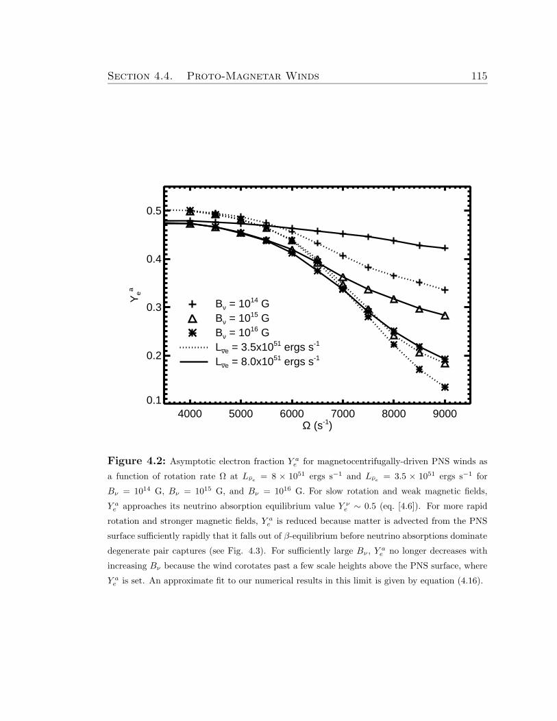
Section 4.4. Proto-Magnetar Winds 115
4000 5000 6000 7000 8000 9000Ω (s-1)
0.1
0.2
0.3
0.4
0.5
Yea
Bν = 1014 GBν = 1015 GBν = 1016 GLνe = 3.5x1051 ergs s-1 _
Lνe = 8.0x1051 ergs s-1 _
Figure 4.2: Asymptotic electron fraction Y ae for magnetocentrifugally-driven PNS winds as
a function of rotation rate Ω at Lνe= 8 × 1051 ergs s−1 and Lνe
= 3.5 × 1051 ergs s−1 for
Bν = 1014 G, Bν = 1015 G, and Bν = 1016 G. For slow rotation and weak magnetic fields,
Y ae approaches its neutrino absorption equilibrium value Y ν
e ∼ 0.5 (eq. [4.6]). For more rapid
rotation and stronger magnetic fields, Y ae is reduced because matter is advected from the PNS
surface sufficiently rapidly that it falls out of β-equilibrium before neutrino absorptions dominate
degenerate pair captures (see Fig. 4.3). For sufficiently large Bν , Yae no longer decreases with
increasing Bν because the wind corotates past a few scale heights above the PNS surface, where
Y ae is set. An approximate fit to our numerical results in this limit is given by equation (4.16).
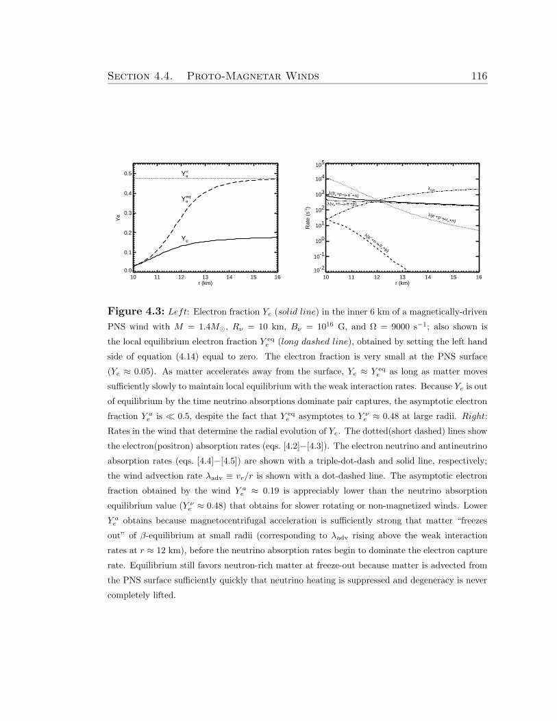
Section 4.4. Proto-Magnetar Winds 116
10 11 12 13 14 15 16r (km)
0.0
0.1
0.2
0.3
0.4
0.5
Ye
Ye
Yeeq
Yeν
10 11 12 13 14 15 16r (km)
10-2
10-1
100
101
102
103
104
105
Rat
e (s
-1)
λ(νe+n e-+p)
λadvλ(νe+p e++n) -
λ(e ++n ν
e +p)
-
λ(e -+p νe+n)
Figure 4.3: Left: Electron fraction Ye (solid line) in the inner 6 km of a magnetically-driven
PNS wind with M = 1.4M¯, Rν = 10 km, Bν = 1016 G, and Ω = 9000 s−1; also shown is
the local equilibrium electron fraction Y eqe (long dashed line), obtained by setting the left hand
side of equation (4.14) equal to zero. The electron fraction is very small at the PNS surface
(Ye ≈ 0.05). As matter accelerates away from the surface, Ye ≈ Y eqe as long as matter moves
sufficiently slowly to maintain local equilibrium with the weak interaction rates. Because Ye is out
of equilibrium by the time neutrino absorptions dominate pair captures, the asymptotic electron
fraction Y ae is ¿ 0.5, despite the fact that Y eq
e asymptotes to Y νe ≈ 0.48 at large radii. Right:
Rates in the wind that determine the radial evolution of Ye. The dotted(short dashed) lines show
the electron(positron) absorption rates (eqs. [4.2]−[4.3]). The electron neutrino and antineutrino
absorption rates (eqs. [4.4]−[4.5]) are shown with a triple-dot-dash and solid line, respectively;
the wind advection rate λadv ≡ vr/r is shown with a dot-dashed line. The asymptotic electron
fraction obtained by the wind Y ae ≈ 0.19 is appreciably lower than the neutrino absorption
equilibrium value (Y νe ≈ 0.48) that obtains for slower rotating or non-magnetized winds. Lower
Y ae obtains because magnetocentrifugal acceleration is sufficiently strong that matter “freezes
out” of β-equilibrium at small radii (corresponding to λadv rising above the weak interaction
rates at r ≈ 12 km), before the neutrino absorption rates begin to dominate the electron capture
rate. Equilibrium still favors neutron-rich matter at freeze-out because matter is advected from
the PNS surface sufficiently quickly that neutrino heating is suppressed and degeneracy is never
completely lifted.
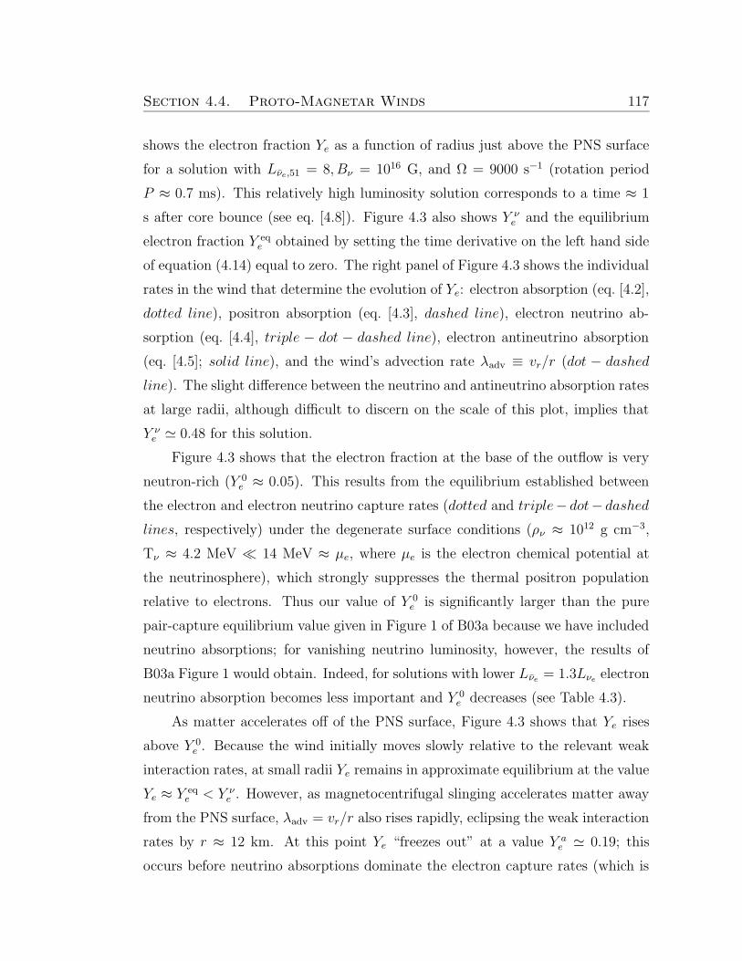
Section 4.4. Proto-Magnetar Winds 117
shows the electron fraction Ye as a function of radius just above the PNS surface
for a solution with Lνe,51 = 8, Bν = 1016 G, and Ω = 9000 s−1 (rotation period
P ≈ 0.7 ms). This relatively high luminosity solution corresponds to a time ≈ 1
s after core bounce (see eq. [4.8]). Figure 4.3 also shows Y νe and the equilibrium
electron fraction Y eqe obtained by setting the time derivative on the left hand side
of equation (4.14) equal to zero. The right panel of Figure 4.3 shows the individual
rates in the wind that determine the evolution of Ye: electron absorption (eq. [4.2],
dotted line), positron absorption (eq. [4.3], dashed line), electron neutrino ab-
sorption (eq. [4.4], triple − dot − dashed line), electron antineutrino absorption
(eq. [4.5]; solid line), and the wind’s advection rate λadv ≡ vr/r (dot − dashed
line). The slight difference between the neutrino and antineutrino absorption rates
at large radii, although difficult to discern on the scale of this plot, implies that
Y νe ' 0.48 for this solution.
Figure 4.3 shows that the electron fraction at the base of the outflow is very
neutron-rich (Y 0e ≈ 0.05). This results from the equilibrium established between
the electron and electron neutrino capture rates (dotted and triple− dot− dashed
lines, respectively) under the degenerate surface conditions (ρν ≈ 1012 g cm−3,
Tν ≈ 4.2 MeV ¿ 14 MeV ≈ µe, where µe is the electron chemical potential at
the neutrinosphere), which strongly suppresses the thermal positron population
relative to electrons. Thus our value of Y 0e is significantly larger than the pure
pair-capture equilibrium value given in Figure 1 of B03a because we have included
neutrino absorptions; for vanishing neutrino luminosity, however, the results of
B03a Figure 1 would obtain. Indeed, for solutions with lower Lνe = 1.3Lνe electron
neutrino absorption becomes less important and Y 0e decreases (see Table 4.3).
As matter accelerates off of the PNS surface, Figure 4.3 shows that Ye rises
above Y 0e . Because the wind initially moves slowly relative to the relevant weak
interaction rates, at small radii Ye remains in approximate equilibrium at the value
Ye ≈ Y eqe < Y ν
e . However, as magnetocentrifugal slinging accelerates matter away
from the PNS surface, λadv = vr/r also rises rapidly, eclipsing the weak interaction
rates by r ≈ 12 km. At this point Ye “freezes out” at a value Y ae ' 0.19; this
occurs before neutrino absorptions dominate the electron capture rates (which is
Section 4.4. Proto-Magnetar Winds 118
why Ye ≈ Y eqe is still relatively low).
4.4.3 Conditions for Neutron-Rich Outflows from Proto-
Magnetars
The mass-loss rate for purely thermal, neutrino-driven PNS winds Mth can be
derived analytically by requiring that the energy used to unbind a typical nucleon
EB = GMmn/Rν be supplied entirely by the neutrino heating Qν ≡∫∞
Rνqνdr/vr
that a nucleon experiences in accelerating from the PNS surface to large radii
(QW96), where qν is the net neutrino heating rate per baryon, which is dominated
by neutrino absorption (eqs. [4.4]−[4.5]). By repeating this derivation but instead
requiring that Qν . 〈εν〉 (see §4.2) we obtain the minimum mass-loss rate that
must accompany a neutron excess over the neutrino-driven value
M
Mth
& φn ≡GMmn
Rν〈εν〉≈ 20M1.4〈ενe,10〉
−1R−110 , (4.18)
where (QW96)
Mth ≈ 10−6L5/3νe,51〈ενe,10〉
10/3M−21.4R
5/310 M¯ s
−1, (4.19)
Rν = 10R10 km, M = 1.4M1.4M¯, and 〈εν〉 ≈ 〈ενe〉 = 10〈ενe,10〉 MeV. In our
numerical calculations we have assumed that Lν ∝ 〈εν〉4 so that Mth ∝ L
5/2ν .
In Figure 4.4 we show M for the same wind solutions for which Y ae is shown in
Figure 4.2. Figure 4.4 shows that M is substantially enhanced over its thermally-
driven value Mth in the presence of a strong magnetic field and rapid rotation.
This enhanced mass-loss occurs because a strong magnetic field forces the outflow
to corotate above the PNS surface and rapid corotation brings the wind’s sonic
radius Rs much closer to the surface, into the corotating region; this increases
the hydrostatic scale height and the wind density at Rs, thereby increasing M .
Because the magnetic field, as opposed to neutrinos, is primary responsible for
unbinding matter from a rapidly rotating proto-magnetar, the outflow can have
M > Mthφn and can thus remain neutron-rich. Indeed, Figure 4.4 shows that M
Section 4.4. Proto-Magnetar Winds 119
increases exponentially with Ω and a comparison with Figure 4.2 shows that Y ae
first noticeably decreases below Y νe once equation (4.18) is satisfied.
Figure 4.4 also shows that for modest magnetic field strengths M increases
with increasing Bν , but that for sufficiently large Bν , M saturates to a value
Mcf in the “centrifugal limit” (e.g., Lamers & Cassinelli 1999). For Ω ≈ Ωn (or,
equivalently, Y ae ≈ 0.25) we find that
Mcf(Ωn) ≈ 6× 10⁻²(Lνe,51/8)2.2M¯ s
−1, (4.20)
which is over an order of magnitude greater than the mass-loss required, Mthφn ≈
3× 10⁻³(Lνe,51/8)2.25M¯ s
−1 (eq. [4.18]), for just a mild neutron excess relative to
the neutrino-driven value (i.e., Y ae . Y ν
e ).
Figures 4.2 and 4.4 show that at fixed Ω, M → Mcf and Y ae → Y a,sat
e
(eq. [4.16]) for similar magnetic field strengths. To understand why this occurs
note that the requirement for fully centrifugally-enhanced mass-loss is that the
magnetic field must be sufficiently strong to enforce corotation beyond the radius
where M is set; because a wind approximately corotates to its Alfven radius RA
and its mass-loss rate is set at its sonic radius Rs the condition for M → Mcf is
that RA & Rs. In analogy, because Y ae obtains near the PNS surface (see Fig. 4.3),
the condition for Y ae → Y a,sat
e is that RA & Rν . In the centrifugal limit the
sonic radius for an equatorial wind is given by Rs = (GM/Ω2)1/3 (e.g., Lamers &
Cassinelli 1999), so that Rs(Ωn) ≈ 13 km ∼ Rν . Thus the conditions for fully en-
hanced mass-loss and fully enhanced neutron-richness are approximately the same
because the sonic radius is close to the PNS surface for the near break-up rotation
rates required to produce neutron-rich outflow.
Finally, although we have focused on equatorial proto-magnetar winds, the
properties of the outflow will vary with latitude. In particular, M and Y ae will
decrease and increase with increasing angle θ from the equator, respectively, ap-
proaching Mth and Y νe for nearly polar outflow (θ → 90) because of the reduced
centrifugal acceleration along nearly vertical field lines (M and Mth here are per
solid angle). Thus, it may seem plausible that outflows driven from intermediate
latitudes could maintain moderately low Ye yet become significantly more rela-
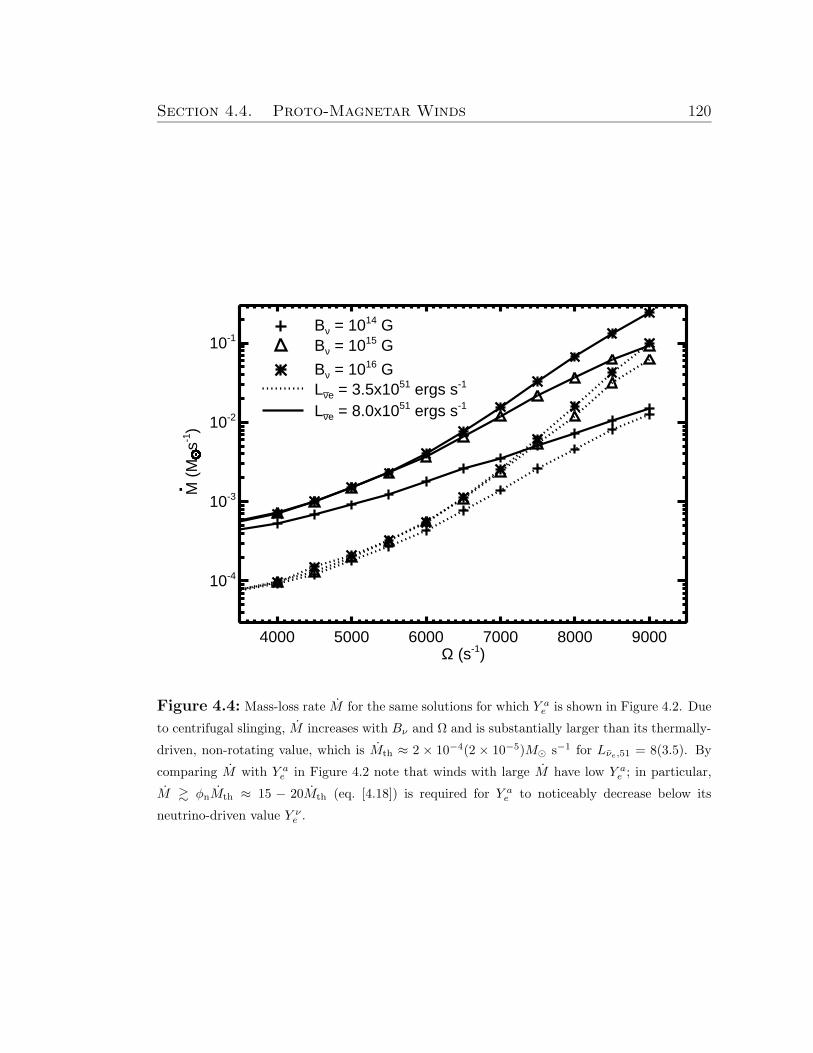
Section 4.4. Proto-Magnetar Winds 120
4000 5000 6000 7000 8000 9000Ω (s-1)
10-4
10-3
10-2
10-1
M (
M s
-1)
Bν = 1014 GBν = 1015 G
Bν = 1016 GLνe = 3.5x1051 ergs s-1 _
Lνe = 8.0x1051 ergs s-1 _
........................................................................................................................................................................................................................................................................................................................................................................................................................................................................................................................................................................................................................................................................................................................................................................................................................................................................................................................................................................................................................................................................................................................................................................................................................................................................................................................................................................................................................................................................................................................................................................................................................................................................................................................................................................................................................................................................................................................................................................................................................................................................................................................................................................................................................................................................................................................................................................................................................................................................................................................................................................................................................................................................................................................................................................................................................................................................................................................................................................................................................................................................................................................................................................................................................................................................................................................................................................................................................................................................................................................................................................................................................................................................................................................................................................................................................................................................................................................................................................................................................................................................................................................................................
.
Figure 4.4: Mass-loss rate M for the same solutions for which Y ae is shown in Figure 4.2. Due
to centrifugal slinging, M increases with Bν and Ω and is substantially larger than its thermally-
driven, non-rotating value, which is Mth ≈ 2 × 10⁻⁴(2 × 10⁻⁵)M¯ s−1 for Lνe,51 = 8(3.5). By
comparing M with Y ae in Figure 4.2 note that winds with large M have low Y a
e ; in particular,
M & φnMth ≈ 15 − 20Mth (eq. [4.18]) is required for Y ae to noticeably decrease below its
neutrino-driven value Y νe .
Section 4.4. Proto-Magnetar Winds 121
tivistic than matter driven from near the equator. Even high-latitude outflows,
however, require M À Mth (eq. [4.18]) to attain Y ae < Y ν
e , making such a scenario
unlikely, as we will show explicitly through NDAF disk wind calculations in §4.5.
Furthermore, the limited solid angle occupied by such a hypothetical mid-latitude
wind would preclude it from carrying a significant portion of the PNS’s spin-down
luminosity, which is primarily extracted by outflow originating near the equator
(e.g., Bucciantini et al. 2006).
4.4.4 Implications for GRBs
We have shown that proto-magnetars born with P < Pn ≈ 0.8 ms produce
energetic, neutron-rich winds; it therefore appears that the birth of very rapidly
rotating proto-magnetars should produce neutron-rich GRBs. This is, however, not
necessarily the case. Even strongly magnetized proto-magnetar winds are baryon-
loaded at very early times following the launch of the SN shock because the PNS is
very hot and its already substantial thermally-driven mass-loss is enhanced due to
centrifugal slinging. In fact, a proto-magnetar requires several seconds to contract
and cool to the point that a wind launched from its surface achieves the high
magnetization σ & 10–100 required to explain the Lorentz factors inferred from
GRBs. By the time a proto-magnetar cools to the point that its wind becomes
ultra-relativistic, it may no longer rotate sufficiently rapidly to remain neutron-
rich.
In Figure 4.5 we explore this possibility quantitatively by showing the magne-
tization σ of a PNS’s outflow (eq. [4.15]) as a function of the PNS rotation period
P from evolutionary calculations of a cooling, spinning down proto-magnetar with
an initial period P0 = 0.6 ms < Pn and for three different fixed surface dipole mag-
netic field strengths:7 Bdipν = 1015 G, 3× 10¹⁵ G, and 1016 G. These evolutionary
7The minimum stable neutron star rotation period Pmin is uncertain theoretically because itdepends on the uncertain supranuclear density equation of state (EOS); depending on the EOS,detailed studies find that Pmin = 0.53 − 1.7 ms for M ' 1.4M¯ (Cook, Shapiro, & Teukolsky1994, Table 8). Thus, although we take the specific value P0 = 0.6 ms in our calculations
Section 4.4. Proto-Magnetar Winds 122
calculations, which are described in more detail in §2.4.1, assume a PNS cooling
evolution similar to that given in equation (4.8) and map the one-dimensional
neutrino-heated monopole wind calculations of Chapter 2 onto a more physical
dipole geometry using the axisymmetric two-dimensional relativistic MHD calcu-
lations of Bucciantini et al. 2006 (hereafter B06). Although Figure 4.5 only shows
calculations for one initial rotation period P0 = 0.6 ms, the PNS’s spin-down
timescale is dominated by times at which it is slowly rotating; hence, the evo-
lutionary tracks for PNSs born with P0 . 0.6 ms are similar to those shown in
Figure 4.5 for P > 0.6 ms, following a brief initial spin-down phase.
Figure 4.5 shows that PNSs born with P < Pn and Bdipν & 3 × 10¹⁵ G spin
down to a relatively neutron-poor state (P > Pn) in just a few seconds, before
cooling sufficiently to produce an ultra-relativistic (σ À 1) outflow; these proto-
magnetars could therefore not produce neutron-rich GRBs. On the other hand,
a PNS born with Bdipν = 1015 G spins down more slowly and is thus capable of
producing an ultra-relativistic, neutron-rich outflow ∼ 10 − 30 seconds following
core bounce. Of the proto-magnetar’s initial rotational energy of Erot ∼ 6 × 1052
ergs, a substantial portion (∼ 2 × 1052 ergs) is extracted when σ < 10 − 100;
although this early wind is potentially too mass-loaded to produce a GRB, it
may enhance the energy and alter the morphology of the accompanying SN shock
(TCQ04; Chapter 2; Bucciantini et al. 2007a). The remaining ∼ 4 × 1052 ergs,
part of which could produce a neutron-rich GRB, emerges when σ > 10−100 on a
somewhat longer spin-down timescale τJ, which is ∼ 102− 103 s, depending on the
fraction of the proto-magnetar’s surface threaded by open magnetic flux (B06).
In §4.3 we emphasized the need for magnetic acceleration to produce neutron-
rich outflows from compact objects. Despite the absence of magnetic fields, how-
ever, Dessart et al. (2006) find neutron-rich (Y ae ∼ 0.25), purely neutrino-driven
outflows in 2D radiation-hydrodynamical simulations of the very early evolution
(t . 800 ms after core bounce) of a rapidly rotating neutron star newly-formed
to illustrate the conditions under which proto-magnetars can produce neutron-rich GRBs, ifPmin > Pn ≈ 0.8 ms the conclusions of this section are much simpler: proto-magnetars cannotproduce neutron-rich outflow. Conversely, the detection of a neutron-rich GRB outflow from aconfirmed magnetar birth would provide a constraint on the EOS.
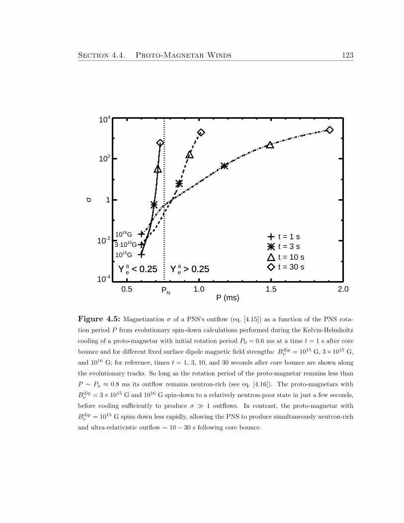
Section 4.4. Proto-Magnetar Winds 123
0.5 1.0 1.5 2.0P (ms)
10-4
10-2
1
102
104
σ
Y e < 0.25Y a < 0.25 Y e > 0.25Y a > 0.25
PN
1015G
3 1015G .1016G t = 1 s
t = 3 st = 10 st = 30 s
Figure 4.5: Magnetization σ of a PNS’s outflow (eq. [4.15]) as a function of the PNS rota-
tion period P from evolutionary spin-down calculations performed during the Kelvin-Helmholtz
cooling of a proto-magnetar with initial rotation period P0 = 0.6 ms at a time t = 1 s after core
bounce and for different fixed surface dipole magnetic field strengths: Bdipν = 1015 G, 3×10¹⁵ G,
and 1016 G; for reference, times t = 1, 3, 10, and 30 seconds after core bounce are shown along
the evolutionary tracks. So long as the rotation period of the proto-magnetar remains less than
P ∼ Pn ≈ 0.8 ms its outflow remains neutron-rich (see eq. [4.16]). The proto-magnetars with
Bdipν = 3×10¹⁵ G and 1016 G spin-down to a relatively neutron-poor state in just a few seconds,
before cooling sufficiently to produce σ À 1 outflows. In contrast, the proto-magnetar with
Bdipν = 1015 G spins down less rapidly, allowing the PNS to produce simultaneously neutron-rich
and ultra-relativistic outflow ∼ 10− 30 s following core bounce.
Section 4.5. Accretion Disk Winds 124
following the accretion-induced collapse (AIC) of a white dwarf. Because these
calculations show that very rapidly rotating PNSs can produce neutron-rich out-
flows without the aid of magnetic acceleration, it may appear that neutron-rich
GRB outflows could be possible under less restrictive conditions than described in
this section. The purely neutrino-driven neutron-rich outflows found by Dessart
et al. (2006) are only possible, however, because at very early times following core
bounce the PNS is inflated with respect to its final, cooled radius and because a
PNS rotating near break-up is strongly oblately deformed. Because the equato-
rial neutrinosphere radius Rν can therefore exceed ∼ 100 km at early times (see
Dessart et al. 2006, Fig. 7), the gravitational binding energy of a nucleon on the
PNS surface at a moderately low latitude is EB ∼ 10(Rν/100 km)−1 MeV, compa-
rable to the mean energy of the neutrinos driving the outflow (typically ≈ 10− 15
MeV during the PNS’s early cooling phase). Thus, despite the fact that neutrino
absorptions favor a proton − rich composition (Y νe > 0.5) because the electron
neutrino flux dominates the electron antineutrino flux during early deleptoniza-
tion (especially in the presence of rapid rotation; Thompson, Quataert, & Bur-
rows 2005), less than a single neutrino is required to unbind a typical nucleon (i.e.,
φn . 1; eq. [4.18]); matter driven from low latitudes can therefore partially retain
the neutron-rich composition of the PNS surface. Although purely neutrino-driven
neutron-rich outflows are thus possible from PNSs at very early times (. 1 s) af-
ter core bounce, as the PNS cools and its radius shrinks φn will increase; purely
neutrino-driven neutron-rich outflows will therefore not be possible after a few
seconds following core bounce, even if the PNS remains distorted by continuing
to rotate near break-up. In particular, once the PNS has cooled and contracted
sufficiently to produce a GRB outflow, neutron-rich winds will only be possible if
they are magnetically-driven and satisfy the constraints described in this section.
4.5 Accretion Disk Winds
In this section we describe calculations of the structure and neutron con-
tent of axisymmetric, one-dimensional MHD winds launched from NDAFs. As
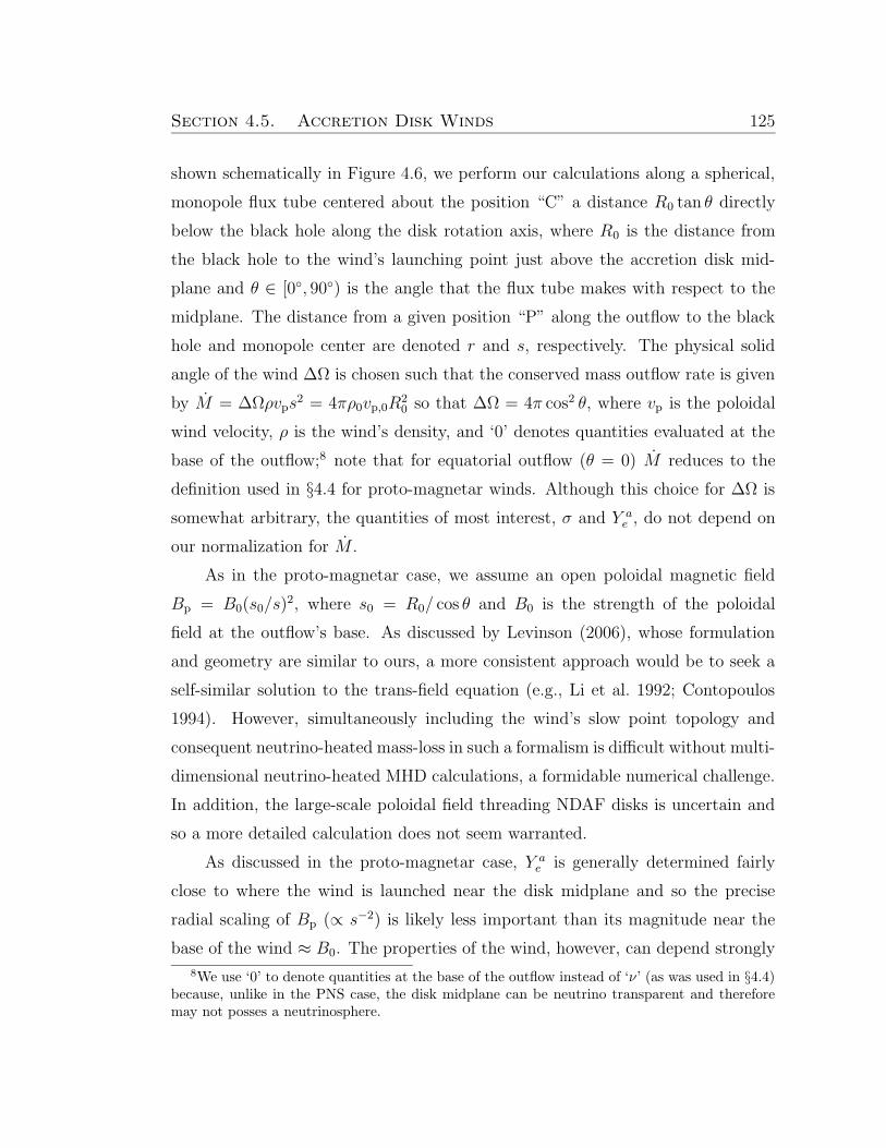
Section 4.5. Accretion Disk Winds 125
shown schematically in Figure 4.6, we perform our calculations along a spherical,
monopole flux tube centered about the position “C” a distance R0 tan θ directly
below the black hole along the disk rotation axis, where R0 is the distance from
the black hole to the wind’s launching point just above the accretion disk mid-
plane and θ ∈ [0, 90) is the angle that the flux tube makes with respect to the
midplane. The distance from a given position “P” along the outflow to the black
hole and monopole center are denoted r and s, respectively. The physical solid
angle of the wind ∆Ω is chosen such that the conserved mass outflow rate is given
by M = ∆Ωρvps2 = 4πρ0vp,0R
20 so that ∆Ω = 4π cos2 θ, where vp is the poloidal
wind velocity, ρ is the wind’s density, and ‘0’ denotes quantities evaluated at the
base of the outflow;8 note that for equatorial outflow (θ = 0) M reduces to the
definition used in §4.4 for proto-magnetar winds. Although this choice for ∆Ω is
somewhat arbitrary, the quantities of most interest, σ and Y ae , do not depend on
our normalization for M .
As in the proto-magnetar case, we assume an open poloidal magnetic field
Bp = B0(s0/s)2, where s0 = R0/ cos θ and B0 is the strength of the poloidal
field at the outflow’s base. As discussed by Levinson (2006), whose formulation
and geometry are similar to ours, a more consistent approach would be to seek a
self-similar solution to the trans-field equation (e.g., Li et al. 1992; Contopoulos
1994). However, simultaneously including the wind’s slow point topology and
consequent neutrino-heated mass-loss in such a formalism is difficult without multi-
dimensional neutrino-heated MHD calculations, a formidable numerical challenge.
In addition, the large-scale poloidal field threading NDAF disks is uncertain and
so a more detailed calculation does not seem warranted.
As discussed in the proto-magnetar case, Y ae is generally determined fairly
close to where the wind is launched near the disk midplane and so the precise
radial scaling of Bp (∝ s−2) is likely less important than its magnitude near the
base of the wind ≈ B0. The properties of the wind, however, can depend strongly
8We use ‘0’ to denote quantities at the base of the outflow instead of ‘ν’ (as was used in §4.4)because, unlike in the PNS case, the disk midplane can be neutrino transparent and thereforemay not posses a neutrinosphere.
Section 4.5. Accretion Disk Winds 126
C
B
!!!!!!!!!!!!!!!!!!!!!!!!!!!!!!!!!!!!!!!!!!!!!!!!!!!!!!!!!!!!!!!!!!!!!!!!!!!!!!!!!!!!!!!!!!!!!!!!!!!!!!!!!!!!!!!!!!!!!!!!!!!!!!!!!!!!!!!!!!!!!!!!!!!!!!!!!!!!!!!!!!!!!!!!!!!!!!!!!!!!!!!!!!!!!!!!!!!!!!!!!!!!!!!!!!!!!!!!!!!!!!!!!!!!!!!!!!!!!!!!!!!!!!!!!!!!!!!!!!!!!!!!!!!!!!!!!!!!!!!!!!!!!!!!!!!!!!!!!!!!!!!!!!!!!!!!!!!!!!!!!!!!!!!!!!!!!!!!!!!!!!!!!!!!!!!!!!!!!!!!!!!!!!!!!!!!!!!!!!!!!!!!!!!!!!!!!!!!!!!!!!!!!!!!!!!!!!!!!!!!!!!!!!!!!!!!!!!!!!!!!!!!!!!!!!!!!!!!!!!!!!!!!!!!!!!!!!!!!!!!!!!!!!!!!!!!!!!!!!!!!!!!!!!!!!!!!!!!!!!!!!!!!!!!!!!!!!!!!!!!!!!!!!!!!!!!!!!!!!!!!!!!!!!!!!!!!!!!!!!!!!!!!!!!!!!!!!!!!!!!!!!!!!!!!!!!!!!!!!!!!!!!!!!!!!!!!!!!!!!!!!!!!!!!!!!!!!!!!!!!!!!!!!!!!!!!!!!!!!!!!!!!!!!!!!!!!!!!!!!!!!!!!!!!!!!!!!!!!!!!!!!!!!!!!!!!!!!!!!!!!!!!!!!!!!!!!!!!!!!!!!!!!!!!!!!!!!!!!!!!!!!!!!!!!!!!!!!!!!!!!!!!!!!!!!!!!!!!!!!!!!!!!!!!!!!!!!!!!!!!!!!!!!!!!!!!!!!!!!!!!!!!!!!!!!!!!!!!!!!!!!!!!!!!!!!!!!!!!!!!!!!!!!!!!!!!!!!!!!!!!!!!!!!!!!!!!!!!!!!!!!!!!!!!!!!!!!!!!!!!!!!!!!!!!!!!!!!!!!!!!!!!!!!!!!!!!!!!!!!!!!!!!!!!!!!!!!!!!!!!!!!!!!!!!!!!!!!!!!!!!!!!!!!!!!!!!!!!!!!!!!!!!!!!!!!!!!!!!!!!!!!!!!!!!!!!!!!!!!!!!!!!!!!!!!!!!!!!!!!!!!!!!!!!!!!!!!!!!!!!!!!!!!!!!!!!!!!!!!!!!!!!!!!!!!!!!!!!!!!!!!!!!!!!!!!!!!!!!!!!!!!!!!!!!!!!!!!!!!!!!!!!!!!!!!!!!!!!!!!!!!!!!!!!!!!!!!!!!!!!!!!!!!!!!!!!!!!!!!!!!!!!!!!!!!!!!!!!!!!!!!!!!!!!!!!!!!!!!!!!!!!!!!!!!!!!!!!!!!!!!!!!!!!!!!!!!!!!!!!!!!!!!!!!!!!!!!!!!!!!!!!!!!!!!!!!!!!!!!!!!!!!!!!!!!!!!!!!!!!!!!!!!!!!!!!!!!!!!!!!!!!!!!!!!!!!!!!!!!!!!!!!!!!!!!!!!!!!!!!!!!!!!!!!!!!!!!!!!!!!!!!!!!!!!!!!!!!!!!!!!!!!!!!!!!!!!!!!!!!!!!!!!!!!!!!!!!!!!!!!!!!!!!!!!!!!!!!!!!!!!!!!!!!!!!!!!!!!!!!!!!!!!!!!!!!!!!!!!!!!!!!!!!!!!!!!!!!!!!!!!!!!!!!!!!!!!!!!!!!!!!!!!!!!!!!!!!!!!!!!!!!!!!!!!!!!!!!!!!!!!!!!!!!!!!!!!!!!!!!!!!!!!!!!!!!!!!!!!!!!!!!!!!!!!!!!!!!!!!!!!!!!!!!!!!!!!!!!!!!!!!
""""""""""""""""""""""""""""""""""""""""""""""""""""""""""""""""""""""""""""""""""""""""""""""""""""""""""""""""""""""""""""""""""""""""""""""""""""""""""""""""""""""""""""""""""""""""""""""""""""""""""""""""""""""""""""""""""""""""""""""""""""""""""""""""""""""""""""""""""""""""""""""""""""""""""""""""""""""""""""""""""""""""""""""""""""""""""""""""""""""""""""""""""""""""""""""""""""""""""""""""""""""""""""""""""""""""""""""""""""""""""""""""""""""""""""""""""""""""""""""""""""""""""""""""""""""""""""""""""""""""""""""""""""""""""""""""""""""""""""""""""""""""""""""""""""""""""""""""""""""""""""""""""""""""""""""""""""""""""""""""""""""""""""""""""""""""""""""""""""""""""""""""""""""""""""""""""""""""""""""""""""""""""""""""""""""""""""""""""""""""""""""""""""""""""""""""""""""""""""""""""""""""""""""""""""""""""""""""""""""""""""""""""""""""""""""""""""""""""""""""""""""""""""""""""""""""""""""""""""""""""""""""""""""""""""""""""""""""""""""""""""""""""""""""""""""""""""""""""""""""""""""""""""""""""""""""""""""""""""""""""""""""""""""""""""""""""""""""""""""""""""""""""""""""""""""""""""""""""""""""""""""""""""""""""""""""""""""""""""""""""""""""""""""""""""""""""""""""""""""""""""""""""""""""""""""""""""""""""""""""""""""""""""""""""""""""""""""""""""""""""""""""""""""""""""""""""""""""""""""""""""""""""""""""""""""""""""""""""""""""""""""""""""""""""""""""""""""""""""""""""""""""""""""""""""""""""""""""""""""""""""""""""""""""""""""""""""""""""""""""""""""""""""""""""""""""""""""""""""""""""""""""""""""""""""""""""""""""""""""""""""""""""""""""""""""""""""""""""""""""""""""""""""""""""""""""""""""""""""""""""""""""""""""""""""""""""""""""""""""""""""""""""""""""""""""""""""""""""""""""""""""""""""""""""""""""""""""""""""""""""""""""""""""""""""""
######
$$$$$$
%%%%%%%%%%%%%%%%%%%%%%%%%%%%%%%%%%%
&&&&&&&&&&&&&&&&&&&&&&&&&&&&&&&&&&&
0s
θ
s
R0
r
P
Figure 4.6: Geometry of NDAF disk winds. The wind is calculated along a flux tube that
is inclined at an angle θ with respect to the accretion disk midplane. The calculation is started
from a location just above the disk midplane a distance R0 from the central black hole and at a
distance s0 from the monopole center (position “C”). A generic point “P” along the outflow is
located at a distance r from the central black hole and a distance s from the monopole center.
Section 4.5. Accretion Disk Winds 127
on θ. In particular for θ < 60 matter that co-rotates at the Keplerian orbital
velocity which is perturbed from the disk along the field line is unstable and
can escape to infinity, even without additional energy deposition (Blandford &
Payne 1982). This results in significant mass-loading for field lines with θ <
60; in addition, the field develops a substantial base toroidal component Bφ,0.
For θ < 60, NDAF winds are therefore slow, heavily mass-loaded, have Bφ,0 À
B0, and possess properties that are relatively independent of θ. On the other
hand, more vertical flux tubes (60 < θ < 90), which resemble equatorial proto-
magnetar winds more than equatorial disk winds, have lower M , accelerate to
faster asymptotic speeds, and possess properties that depend sensitively on θ;
in particular, the wind becomes increasing relativistic as θ → 90 (Daigne &
Mochkovitch 2002), and ultra-relativistic outflows from nearly vertical field lines
may be capable of producing GRBs.
In terms of B0 and M the magnetization (eq. [4.13]) of an NDAF wind
launched from radius R0 is given by
σ = B20R
40Ω
2K/Mc3, (4.21)
where we have assumed that the base of the outflow rotates at approximately the
Keplerian rate ΩK = (GM/R30)
1/2. The rate of angular momentum lost through
a non-relativistic (σ < 1) wind is given by JW = MR2AΩK, while for relativistic
(σ > 1) winds RA ' RL and JW ' Emag/ΩK ' σMc2/ΩK, where Emag is the
wind’s energy-loss rate. The ratio of JW to the disk’s angular momentum-loss rate
JD = MDR20ΩK is therefore given by
JW
JD' (MR2
A/MDR20) = (Ms2A/MDs
20) : σ < 1
' (B20R
20/MDc) : σ > 1 (4.22)
Although a wind with JW < JD is physical because stresses internal to the disk
can transfer angular momentum outwards, allowing accretion at MD to proceed, a
wind for which JW > JD is unphysical because it violates conservation of angular
momentum.
Section 4.5. Accretion Disk Winds 128
4.5.1 Numerical Procedure
We calculate NDAF wind solutions starting from a location just above the
accretion disk midplane at a fixed cylindrical radius R0 = 14Rg ≈ 6 × 106 cm,
which is roughly the location of the disk’s peak neutrino flux. The wind’s local
neutrino luminosities and energies are determined from CB07’s marginally neutrino
optically thin MD = 0.2M¯ s−1, α = 0.03 NDAF solution. We focus on winds
driven from low MD, neutrino transparent disks because low MD accretion, due
to its lower neutrino-driven mass-loss, is probably more likely to produce neutron-
rich, ultra-relativistic outflow. When considering NDAFs with MD < 0.2M¯ s−1
(down to MD ≈ Mign; eq. [4.1]), we scale the boundary conditions and neutrino
emission properties analytically from the MD = 0.2M¯ s−1 solution, as discussed
below.
We use Newtonian gravity, including just the point mass of a M = 3M¯ black
hole. This is a reasonable approximation because our calculation begins at a radius
greater than twice the radius of the innermost stable circular orbit. The evolution
equations for vp, vφ, Bφ, ρ, and T are the same as those used in the PNS case with
r replaced by s, except that the gravitational acceleration in the radial momentum
equation (eq. [2.3]) is now the component projected along the field line:
gs =GM(s− s0 sin
2 θ)
(s2 + sin2 θ[s20 − 2ss0])3/2. (4.23)
Our microphysics is essentially identical to that in the PNS case. In particular,
the electron fraction is evolved according to equation (4.14), again with r replaced
by s; note that because of the disk’s significantly lower density, degeneracy effects
are less important near the base of the wind than in the PNS case. The electron
and anti-electron neutrino energy fluxes (Fνe , Fνe) used to calculate the neutrino
absorption and heating rates near R0 are computed from CB07’s α−disk solution in
the same manner as the local neutrino energy densities that were used to calculate
Y νe for Figure 4.1; to within a factor of ∼ 2 the total spherically-equivalent neutrino
luminosity obeys Lν = Lνe + Lνe ≡ 4πR20(Fνe + Fνe) ≈ ηMDc
2, where η ≈ 0.04 is
the total radiative efficiency for a non-rotating black hole from CB07. In a similar
Section 4.5. Accretion Disk Winds 129
manner as for PNSs, we take the neutrino flux intercepted by the outflow to be
approximately constant with radius for r . R0 and to decrease ∝ r−2 for r & R0
(T01 eq. [24]; see Surman & McLaughlin 2004, 2005 for a more detailed treatment).
Although the geometry that we assume is simplistic, Y ae is set relatively close to
the base of the wind and thus depends primarily on the neutrino energy density in
the vicinity of R0. Indeed, as Figure 4.3 illustrates, the advection and pair capture
rates rise and fall above the base of the outflow, respectively, much more rapidly
than the neutrino absorption rates decrease; this would likely remain true for any
realistic geometry.
Unlike PNSs, NDAFs do not produce significant tau or muon neutrino emis-
sion and so annihilations and neutral-current interactions from these neutrino
species are ignored. The mean electron and anti-electron neutrino energies near R0,
which are not expected to vary strongly with MD for neutrino optically thin accre-
tion (see eq. [4.9]), are taken from Figure 4.1 as 〈ενe〉 = 10.5 MeV and 〈ενe〉 = 13.1
MeV; from CB07’s solution we also determine that Fνe ' 1.2Fνe near R0 so that
Y νe ≈ 0.51 (see eq. [4.6] and Fig. 4.1). We set the wind’s inner density ρ0 equal to
the disk midplane density ρD if the electron neutrino optical depth along s to the
midplane is τν . 23; otherwise, we instead choose ρν to enforce τν '
23at s0.
Although viscous heating generally dominates neutrino heating in the mid-
plane of NDAFs, recent radiation MHD simulations suggest that little energy is
dissipated in the disk corona (Turner 2004; Hirose, Krolik, & Stone 2006; Blaes et
al. 2006b; Krolik et al. 2006). For this reason, we neglect viscous heating in the
wind entirely and set the base temperature T0 of the wind by balancing neutrino
cooling with just neutrino heating, as in the PNS case; note, however, that signif-
icant viscous heating in the wind would likely result in both additional mass-loss
and deneutronization. The disk’s midplane temperature TD, which is set by the
balance between viscous heating and neutrino cooling (see eqs. [4.9]−[4.10]), is
therefore generally higher than T0.
Although NDAFs are efficiently cooled and geometrically-thin, radial pressure
support is not completely negligible and so the disk’s angular rotation frequency
Ω, which we use to set the wind’s inner angular velocity, is slightly sub-Keplerian:
Section 4.5. Accretion Disk Winds 130
Ω2 = Ω2K(1 − H2/R2
0), where H ≈ 0.2R0 is the disk scale height near R0, which,
like TD, is approximately independent of MD for neutrino optically thin accretion.
Our disk wind calculations can be compared with similar one-dimensional
flux tube calculations by Daigne & Mochkovitch 2002 (DM02), Pruet et al. 2004
(P04), and Levinson 2006 (L06). DM02 calculated the requisite conditions for
ultra-relativistic outflow from hyper-accreting disks, including neutrino heating
and cooling and, in the neutrino optically thin case, a simplified viscous heating
prescription. Because DM02 was primarily concerned with obtaining M as a func-
tion of disk conditions, they only considered wind conditions near the sonic point;
in addition, DM02 assumed co-rotation rather than accounting for the magnetic
field explicitly. L06 improved upon the calculations of DM02 by including the full
equations of general relativistic MHD. Although L06 explored the effects of finite
B0, L06 concentrated, like DM02, on the sub-slow magnetosonic regime and his
calculations did not capture the Alfven or fast magnetosonic radii. Although this
approach allowed L06 to calculate M as a function of the open magnetic flux and
Lν , the base toroidal field Bφ,0 remained a free parameter in L06’s formulation.
Because Bφ,0 is associated with the conserved magnetic induction it is fixed in
our calculations by the fact that our steady-state winds pass smoothly through
all three MHD critical points. L06 speculated on the potential deneutronization
of magnetized NDAF winds by noting the similarity between the advection and
relevant weak interaction rates; he did not, however, calculate the evolution of Ye
explicitly.
Finally, P04 investigated nucleosynthesis in collapsar disk winds by solving the
equations of hydrodynamics and by evolving Ye from the disk midplane. P04 in-
cluded neutrino heating and viscous heating through an α−prescription; although
they neglected neutrino absorptions in evolving Ye, they also argued for the generic
deneutronization of thermally-driven winds. Although P04 did not include the ef-
fects of magnetic fields on the wind explicitly, their outflows were calculated along
well-defined, vertically-directed flux tubes and were artificially forced to co-rotate
outside the base of the wind, presumably to mimic the effect of a strong poloidal
magnetic field. Our calculations are, to the best of our knowledge, the first to fully
Section 4.5. Accretion Disk Winds 131
calculate the effects of MHD on the evolution of Ye in NDAF outflows and the first
to capture all three MHD critical points.
4.5.2 Numerical Results
The solid lines in Figure 4.7 show calculations of the mass-loss rate M , asymp-
totic electron fraction Y ae , magnetization σ (eq. [4.21]), and angular momentum-
loss rate JW compared to that required for accretion JD (eq. [4.22]) for NDAF
winds with base poloidal field B0 = 1013 G, 1014 G, and 1015 G as a function
of flux tube angle θ for the MD = 0.2 M¯ s−1, α = 0.03, M = 3M¯, a = 0
NDAF solution of CB07 (the solution on which Figure 4.1 was based). Because
magnetic pressure at the base of the outflow exceeds the total thermal pressure in
the midplane of the disk for B0 & 2× 10¹⁵ G, fields much stronger than those we
have considered in Figure 4.7 are probably unphysical because they could not be
self-consistently anchored to the disk. Our disk wind calculations are summarized
in Table 4.4.
Figure 4.7 shows that M is very large and relatively independent of θ for
θ . 60 but that for θ & 60 M decreases rapidly with increasing θ. The mass-loss
rate also increases with increasing B0, except for the largest angles, for which M
saturates for sufficiently large B0, no longer increasing with increasing B0 (as in
the PNS case; see Fig. 4.4). There is no similar saturation for smaller θ because
the large values of M preclude the outflow from co-rotating out to the sonic point
for physical B0.9
Figure 4.7 also shows that although Y ae is relatively low (∼ 0.3) for the high-
B0, low-θ wind solutions, all of the solutions in Figure 4.7 with Y ae ¿ Y ν
e ' 0.51
are unphysical because they have JW > JD and thus extract angular momentum
at a rate exceeding that required for accretion through the disk from which the
wind’s boundary conditions were derived; in fact, invoking the criterion JW < JD9Because the base of the wind rotates at a slightly sub-Keplerian rate due to radial pressure
support in the disk, even for θ < 60 mass-loss would saturate at M ≈ 4πR20ρ0cs,0 ∼ 10−100M¯
s−1 for sufficiently large B0 (∼ 1016 G; the co-rotating limit), where cs,0 ∼ 0.1 c is the soundspeed near the base of the outflow.
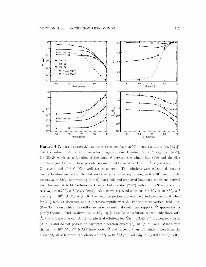
Section 4.5. Accretion Disk Winds 132
50 60 70 80 90θ (degrees)
10-5
10-4
10-3
10-2
10-1
1
10 M
(M
s-1)
1013 G
1014 G1015 G
= 0.20 M s-1MD
.
= 0.01 M s-1MD
.
........................................................................................................................................................................................................................................................................................................................................................................................................................................................................................................................................................................................................................................................................................................................................................................................................................................................................................................................................................................................................................................................................................................................................................................................................................................................................................................................................................................................................................................................................................................................................................................................................................................................................................................................................................................................................................................................................................................................................................................................................................................................................................................................................................................................................................................................................................................................................................................................................................................................................................................................................................................................................................................................................................................................................................................................................................................................................................................................................................................................................................................................................................................................................................................................................................................................................................................................................................................................................................................................................................................................................................................................................................................................................................................................................................................................................................................................................................................................................................................................................................................................................................................................................................
.........................................................................................................................................................................................................................................................................................................................................................................................................................................................................................................................................................................................................................................................................................................................................................................................................................................................................................................................................................................................................................................................................................................................................................................................................................................................................................................................................................................................................................................................................................................................................................................................................................................................................................................................................................................................................................................................................................................................................................................................................................................................................................................................................................................................................................................................................................................................................................................................................................................................................................................................................................................................................................................................................................................................................................................................................................................................................................................................................................................................................................................................................................................................................................................................................................................................................................................................................................................................................................................................................................................................................................................................................................................................................................................................................................................................................................................................................................................................................................................................................................................................................................................................................................
........................................................................................................................................................................................................................................................................................................................................................................................................................................................................................................................................................................................................................................................................................................................................................................................................................................................................................................................................................................................................................................................................................................................................................................................................................................................................................................................................................................................................................................................................................................................................................................................................................................................................................................................................................................................................................................................................................................................................................................................................................................................................................................................................................................................................................................................................................................................................................................................................................................................................................................................................................................................................................................................................................................................................................................................................................................................................................................................................................................................................................................................................................................................................................................................................................................................................................................................................................................................................................................................................................................................................................................................................................................................................................................................................................................................................................................................................................................................................................................................................................................................................................................................................................
50 60 70 80 90θ (degrees)
0.1
0.2
0.3
0.4
0.5
Yea
50 60 70 80 90θ (degrees)
10-5
10-4
10-3
10-2
10-1
1
10
102
σ
50 60 70 80 90θ (degrees)
10-3
10-2
10-1
1
10
102
J Win
d/J D
isk
.
.
Figure 4.7: mass-loss-rate M , asymptotic electron fraction Y ae , magnetization σ (eq. [4.21]),
and the ratio of the wind to accretion angular momentum-loss rates JW /JD (eq. [4.22])
for NDAF winds as a function of the angle θ between the wind’s flux tube and the disk
midplane (see Fig. 4.6); base poloidal magnetic field strengths B0 = 1013 G (asterisk), 1014
G (cross), and 1015 G (diamond) are considered. The solutions were calculated starting
from a location just above the disk midplane at a radius R0 = 14Rg ≈ 6 × 106 cm from the
central M = 3M¯, non-rotating (a = 0) black hole and employed boundary conditions derived
from the α−disk NDAF solution of Chen & Beloborodov (2007) with α = 0.03 and accretion
rate MD = 0.2M¯ s−1 (solid lines). Also shown are wind solutions for MD ≈ 10−2M¯ s−1
and B0 = 1014 G. For θ . 60 the wind properties are relatively independent of θ while
for θ & 60, M decreases and σ increases rapidly with θ. For the most vertical field lines
(θ → 90), along which the outflow experiences minimal centrifugal support, M approaches its
purely thermal, neutrino-driven value Mth (eq. [4.24]). Of the solutions shown, only those with
JW /JD < 1 are physical. All of the physical solutions for MD = 0.2M¯ s−1 are non-relativistic
(σ < 1) and do not possess an asymptotic neutron excess (Y ae ≈ Y ν
e ' 0.51). Winds from
the MD = 10−2M¯ s−1 NDAF have lower M and larger σ than the winds driven from the
higher MD disk; however, the solutions for MD = 10−2M¯ s−1 with JW < JD still have Y ae ∼ 0.5.
Section 4.5. Accretion Disk Winds 133
(see eq. [4.22]), the only physical solutions in Figure 4.7 are those with B0 = 1013
G for all θ and B0 = 1014 G for θ & 80. Also note from Figure 4.7 that, in
addition to having Y ae ∼ 0.5, all of the physical solutions for MD = 0.2M¯ s−1
are non-relativistic (σ < 1). Because our calculations have thoroughly spanned
the physical parameter space of B0 and θ, this conclusion is robust, at least for
MD = 0.2M¯ s−1.
For lower MD the deneutronizing neutrino luminosity and neutrino-driven
mass-loss rate are lower and thus relativistic, neutron-rich outflow may be more
likely. To explore this possibility we have also calculated wind solutions for outflows
driven from an NDAF with MD = 10−2M¯ s−1 ' Mign(α = 0.03), keeping the
other parameters identical to those of the higher MD case (α = 0.03, M = 3M¯,
R0 = 14Rg). To compute these low MD solutions we decreased the neutrino
fluxes by a factor of 20 from our MD = 0.2M¯ s−1 calculation, left the mean
neutrino energies unchanged (they are not expected to vary strongly with MD;
see eq. [4.9]), and decreased the disk midplane density ρ0 ∼ ρD ∝ MD. We only
calculated solutions with B0 . 3 × 10¹⁴ G because for larger field strengths the
magnetic pressure would exceed the thermal pressure in the disk.
In Figure 4.7 we show the MD = 10−2M¯ s−1 calculations for B0 = 1014
G with a dotted line for comparison with the higher MD solutions. Although the
properties of these low MD winds and their dependence on θ qualitatively resemble
the higher MD solutions, Y ae and M are generally lower and σ is higher than for
the winds driven from the more neutrino-luminous disk. Most notably, the high-θ
solutions are now both physical (JW < JD) and relativistic (σ > 1), illustrating
that nearly vertically-directed outflows from low-MD NDAFs represent plausible
GRB central engines. However, these high-θ, relativistic winds still possess no
significant neutron excess (Y ae ∼ 0.5); this means that, even for MD ≈ Mign,
simultaneously neutron-rich and ultra-relativistic outflow appears unlikely. One
might think that MD (and hence Lν) could be lowered further until neutron-
rich, ultra-relativistic outflow was possible at some intermediate latitude; a key
difference, however, between the NDAF problem considered here and the PNS
problem considered in §4.4 is that, unlike in the PNS case, the disk’s neutrino
Section 4.5. Accretion Disk Winds 134
luminosity cannot be decreased below Lν,ign = ηMign(α = 0.03)c2 ∼ 1051 ergs s−1
(eq. [4.7]). For MD < Mign the disk is geometrically thick, and the midplane is not
necessarily degenerate and neutron-rich (see §4.5.5).
4.5.3 Analytic Constraints
As in the PNS case, the purely thermal, neutrino-driven mass-loss rate from
NDAFs can be estimated analytically by requiring that the energy used to unbind
a typical nucleon EB be supplied entirely by neutrino heating; equation (4.19)
can therefore also be used to estimate Mth for NDAF disk winds, provided that
Rν → R0, 〈εν〉 is taken from equations (4.9) and (4.10), and that, as discussed
below, we include the effects of the lower effective gravity geff near the base of the
outflow than in the PNS case. For neutrino optically thin accretion we find that
Mth for NDAFs is given by
Mth ≈ 10−3
(
MD
Mign
)5/3(
geff/(GM/R20)
H/R0
)−1
M119/903 α
301/900.1
(
Rp
6Rg
)−1(R0
6Rg
)79/60
M¯ s−1 (4.24)
where we have used equation (4.7) to scale the neutrino luminosity to the value
Lν,ign associated with the ignition accretion rate Mign (eq. [4.1]) because NDAFs
only exist for MD > Mign.
The purely neutrino-driven mass-loss rate for PNSs (eq. [4.19]) was derived
for outflows emerging antiparallel to the PNS’s gravitational field and by assuming
substantially sub-break-up rotation. NDAF winds, however, are driven from the
disk midplane at an angle inclined with respect to the black hole’s gravitational
field (i.e., θ 6= 0) and even non-magnetized centrifugal support can be important
near the base of the outflow because the disk rotates at nearly the Keplerian
rate. This means that the effective surface gravity geff(θ), which is the difference
between the gravitational acceleration inward along s (gs(θ); eq. [4.23]) and the
centrifugal acceleration outward along s (v2φ/s), is always less than the gravitational
acceleration for purely equatorial outflow (gs(θ = 0) = GM/R20) that was used to
Section 4.5. Accretion Disk Winds 135
derive Mth for PNSs. Assuming that the wind conserves angular momentum away
from s0 (i.e., vφ = ΩR0(s/s0)−1) and concentrating on the wind’s inner, quasi-
hydrostatic atmosphere, we find that geff/(GM/R20) is roughly constant with θ and
is approximately equal to (H/R0) ≈ 0.3α1/100.1 M
−1/103 (R0/6Rg)
7/20, where H is the
NDAF’s vertical scale height near R0; this calculation justifies our characteristic
scaling for geff in equation (4.24).
Although equation (4.24) represents the thermal, neutrino-driven mass-loss
rate from an NDAF, only the nearly-vertical, θ = 89 wind solutions shown in
Figure 4.7 (which experience minimal centrifugal support) in fact reach M ∼ Mth.
Thus, equation (4.24) should be taken as the absolute minimum NDAF mass-loss
rate; in the presence of even a modest magnetic field with a non-vertical inclination,
M is significantly larger that Mth. Because NDAFs possess an absolute minimum
mass-loss rate, their outflows also posses an absolute maximum magnetization
σmax, which is given by
σmax =B2
0Ω2KR
40
Mthc3≈ 10(αβφ)
−1
(
βφβp
)
(
MD
Mign
)−2/3(
geff/(GM/R20)
H/R0
)
×M1/93 α
−16/90.1
(
Rp
6Rg
)23/20(R0
6Rg
)−199/60
, (4.25)
where βp is the ratio of the disk’s midplane thermal pressure PD to the magnetic
pressure associated with the wind’s base poloidal field B20/8π and βφ is similarly
defined for the disk’s midplane toroidal magnetic field Bφ,D. In equation (4.25) we
have written σmax in terms of (αβφ)−1 because for angular momentum transport
via the MRI, local shearing box simulations find that αβφ ∼ 1 (Hawley, Gammie, &
Balbus 1995); we also write equation (4.25) in terms of βφ/βp = B20/B
2φ,D because
if the open poloidal field is generated through a dynamo from the toroidal field
this ratio is unlikely to exceed unity (and is probably much less).
Equation (4.25) shows that σmax ∝ M−2/3D , which explains why the low MD
solutions in Figure 4.7 produced more relativistic outflows than the high MD so-
lutions under the physical constraint βp > 1 that we imposed on our calculations.
Equation (4.25) also shows that NDAFs can, in principle, produce ultra-relativistic
(σ À 102− 103) outflows from small radii (R0 ∼ Risco), provided that a significant
Section 4.5. Accretion Disk Winds 136
fraction of the magnetic energy present in the disk is associated with a large-scale,
open poloidal field (i.e., βp ∼ βt). For α = 0.1, M = 3M¯, βp = βφ, αβφ = 1, and
for accretion onto a rapidly rotating black hole (so that R0 ≈ Rp ≈ 2Rg) equation
(4.25) gives σmax ≈ 102(MD/Mign)−2/3. In this case ultra-relativistic outflow could
occur for MD ∼ Mign and could thus accompany a substantial accretion power
Eacc ≡ ηMDc2 ∼ ηMign(α = 0.1)c2 ∼ 1051 ergs s−1. Because Eacc represents the
maximum MHD luminosity of a GRB-producing jet, this shows that, under ideal
conditions, disk winds from NDAFs form plausible GRB central engines.
Equation (4.25) shows that under some circumstances ultra-relativistic out-
flow from NDAF disks is plausible. However, the maximum magnetization for
material with a neutron excess σnmax is lower than σmax because the minimum
mass-loss rate that must accompany a neutron excess is substantially larger than
Mth according to the same arguments that were used in §4.4.3 for the PNS case;
indeed, using equation (4.25) and the NDAF analog of equation (4.18) we find that
σnmax ≡σmax〈εν〉2R0
GMmn
≈ 2(αβφ)−1
(
βφβp
)
(
MD
Mign
)−2/3(
geff/(GM/R20)
H/R0
)
×M−4/453 α
−71/450.1
(
Rp
6Rg
)17/20(R0
6Rg
)−139/60
. (4.26)
Equation (4.26) shows that neutron-rich, relativistic outflow is very unlikely from
NDAF disks. For MD = Mign, α = 0.1, M = 3M¯, βp = βφ, αβφ = 1, and for
outflow launched from near Risco of a rapidly spinning black hole (R0 = Rp =
2Rg), equation (4.26) gives σnmax ∼ 10, insufficient to explain the ultra-relativistic
outflows inferred from GRBs.
If the fiducial scalings of equation (4.26) are not adopted, ultra-relativistic
outflow with a neutron excess may be possible in some circumstances. For in-
stance, if α = 0.01 instead of α = 0.1 (again for MD = Mign, M = 3M¯,
βp = βφ, αβφ = 1, R0 = Rp = 2Rg) then σnmax ∼ 102 − 103. In this case,
however, Eacc(α = 0.01) ∼ 1050(MD/Mign) ergs s−1 and so a very large fraction of
the accretion energy would need to be deposited in the ultra-relativistic outflow
to explain the observed luminosities of GRBs. Likewise, although αβp ¿ 1 is
Section 4.5. Accretion Disk Winds 137
possible if the poloidal field threading the disk is not the result of a local dynamo
(instead resulting from, e.g., magnetic flux advected from large radii in the disk;
e.g., Spruit & Uzdensky 2005), the constraint JW < JD (eq. [4.22]) independently
requires that αβp & 2/3(R0/Rg)−1/2(R0/H) ≈ 4α
−1/100.1 M
1/103 (R0/Rg)
−17/20; thus,
outflow launched from near Risco must have βpα & 1 because otherwise it would
carry away angular momentum at a rate exceeding that required for matter to ac-
crete at the rate MD. Lastly, we reiterate that the true thermally-driven mass-loss
rate can, in principle, far exceed the purely neutrino-driven value Mth (eq. [4.24])
if viscous heating is important near the base of the wind; if this were the case, σnmax
would be substantially reduced below the value given by equation (4.26). We thus
conclude that neutron-rich GRB outflows are unlikely from NDAF disk winds.
4.5.4 Cross-Field Neutron Diffusion
In the previous section we have argued that highly relativistic (σ & 100−1000)
winds driven from the innermost radii of NDAFs are unlikely to be intrinsically
neutron-rich. However, free neutrons are uncharged and may collisionally diffuse
across magnetic field lines to the polar region (hereafter, the “jet”) from an adja-
cent, more baryon-rich wind (Eichler & Levinson 1999; Levinson & Eichler 2003,
hereafter LE03; McKinney 2005b). If the total neutron mass diffusion rate Mdiffn
dominates the mass-loading of the polar jet then the highly relativistic polar out-
flow will be significantly “polluted” by neutrons and may end up neutron-rich after
all.
Neutron diffusion into the polar jet from the adjacent mass-loaded wind is
limited to a surface area ∼ 4πs2αϕ, where sα is the distance from the base of the
wind to where free nucleons recombine into α−particles (which are charged and
therefore cannot efficiently diffuse across field lines) and we have assumed that
sα À R0/ϕ, where ϕ = π/2 − θ ¿ 1 is the opening angle of the jet. Neutron
diffusion is limited by elastic proton collisions, with a rate 〈σn−pvrel〉 ' 10−15
cm3 s−1 and a corresponding mean free path λn−p ' vth/(np〈σn−pvrel〉), where np
and vth ≈ (kT/mn)1/2 are the proton number density and the ion thermal speed,
Section 4.5. Accretion Disk Winds 138
respectively. Following LE03, we assume that the density gradient length scale
separating the mass-loaded wind and the axial jet is given by l ∼ (vthτdynλn−p)1/2,
where τdyn ≡ s/vp is the wind’s dynamical timescale.10 Using the number flux of
neutrons diffusing into the jet of Fn ≈ nnvth(λn−p/l), we estimate that
Mdiffn ∼ 4πϕs2αmnFn|sα =
(
4πsαkTαM
〈σn−pvrel〉
)1/2
∼ 10−8(
kTαMeV
)1/2( sα108 cm
)1/2(
M
0.1M¯ s−1
)1/2
M¯s−1
(4.27)
where M ≈ 4πϕ2mnvp(np + nn)s2, nn, and Tα ≡ T (sα) are the wind’s mass-
loss rate, neutron number density, and temperature at α−particle recombination,
respectively, and we have assumed that Ye ' 0.5 in the wind. We evaluate equation
(4.27) at sα because Mdiffn is dominated by the largest radii at which the wind is
still primarily free nucleons.
For the relatively moderate entropies (Sa . 102 kB baryon−1) that character-
ize neutrino-heated, magnetocentrifugally-driven winds (see Tables 4.3 and 4.4),
α−particles form at a high temperature (Tα ∼ 1 MeV), which obtains relatively
close to the base of the wind (sα . 107 cm). In this case, even for M ∼ M¯ s−1,
equation (4.27) gives Mdiffn . 10−8M¯ s−1. If the axial jet is itself driven from the
disk, Mdiffn is thus significantly lower than the minimum mass-loss already supplied
by neutrino heating (eq. [4.24]); hence, cross-field neutron diffusion is ineffective
at segregating neutrons in low entropy NDAF winds.
If, on the other hand, the axial jet is powered by ν − ν annihilation or the
Blandford-Znajek process and has little or no intrinsic baryon-loading (such as if it
threads the black hole’s event horizon), then Mdiffn , although small, may dominate
the mass loading of the jet. For instance, for a polar jet power of E ∼ 1050 − 1051
10This choice for l is appropriate for a very abrupt transition in the wind’s density withcylindrical radius, such as between field lines threading the disk and those threading the blackhole’s event horizon. A perhaps more natural (but less conservative) choice for l is the cylindricalradius in the wind at α−particle recombination (≈ ϕsα), which would produce an even smallerMdiff
n than is given in equation (4.27).
Section 4.5. Accretion Disk Winds 139
erg s−1 equation (4.27) shows that diffusive neutron mass-loading from an encasing
wind with a mass-loss rate M ∼ 10−2M¯ s−1 would, by itself, limit the jet’s asymp-
totic Lorentz factor to Γ ∼ 104 − 105. Asymptotically neutron-rich outflow may
result in this case if the jet remains “clean” to large radii; elucidating the observ-
able consequences of such very high-Γ neutron-rich outflows will, however, require
additional work. Lastly, we note that although our calculations show that NDAF
winds probably possess moderate entropy, previous works that have considered
diffusion into the jet have focused on very high entropy outflows characteristic of
hydrodynamic “fireballs” in the GRB literature (LE03; McKinney 2005b). These
calculations find larger Mdiffn than we have estimated in equation (4.27) in large
part because α−particles do not form until much larger radii in high entropy winds.
Furthermore, if Y ae . 0.5 in the encasing baryon-rich wind and some neutrons re-
main free to radii larger than sα, Mdiffn may be larger than predicted by equation
(4.27). Evaluating the free neutron fraction that remains in magnetically-driven
disk winds following the freeze-out of any α-process or r-process capture that may
occur following α−particle recombination is, however, beyond the scope of this
paper.
4.5.5 Thick Accretion Disk Winds
For both proto-magnetars, where Lν ∝ t−1 starting ∼ 1 s following core
bounce (eq. [4.8]), and NDAFs, where Lν ∝ MD ∝ t−5/3 is expected at late
times from “fall-back” accretion (Chevalier 1989; Woosley & Weaver 1995) or
MD ∝ t−α with α ∼ 1 due to the viscous evolution of a disk of finite mass,
the low neutrino luminosities attained at late times are the most favorable for
ultra-relativistic, neutron-rich outflows. However, while proto-magnetars must
maintain sub-millisecond rotation for most of the Kelvin-Helmholtz cooling epoch
to produce late-time neutron-rich GRB outflows, for NDAFs, which always rotate
at nearly the Keplerian rate, the difficulty is more fundamental; for Lν . Lν,ign
(eq. [4.7]) the disk is no longer efficiently cooled and the disk midplane may no
longer remain dense, degenerate, and neutron-rich. For both collapsars and the
Section 4.5. Accretion Disk Winds 140
accretion accompanying compact object mergers there will thus come a time tign
after which MD < Mign and the disk will transition from an NDAF to an advection-
dominated thick disk (Narayan & Yi 1994; Narayan et al. 2001).
Although NDAFs enter β-equilibrium on an accretion timescale (B03a), thick
disks generally do not. Using equation (48) from B03a we find that weak equilib-
rium is only established in a thick disk at radii smaller than a critical β-equilibrium
radius Rβ, which is given by
Rβ = 34(14)(MD/Mign)10/13α
−4/390.1 M
4/393 Rg (4.28)
for accretion onto a black hole with spin a = 0(0.95). Since Rβ < Risco for
MD . 0.1(0.03)Mign, equation (4.28) shows that matter accreting through a thick
disk at a rate MD ¿ Mign is not in weak equilibrium at any radius. The neutron
content of the disk at small radii for tÀ tign (and thus of any potential late-time
GRB-producing outflow) will therefore depend on the composition of the matter
feeding it. In particular, late-time GRB outflows from collapsar disks, which are
continually fed from large radii by their progenitor’s stellar He envelope (which
has Ye ∼ 0.5), will not be neutron-rich.
On the other hand, accretion disks formed from compact object mergers,
which are usually fed from the tidal disruption of at least one neutron star11 (e.g.,
Rosswog & Ramirez-Ruiz 2002), are initially neutron-rich. However, the disks
formed from compact object mergers are expected to be more compact than collap-
sar disks (with circularization radii . 10−30Rg) and are probably not continually
supplied with substantial mass from large radii; the late-time neutron content of
thick disks from compact object mergers therefore depends on the evolution of Y De
immediately following the NDAF to thick disk transition at tign. Since equation
(4.28) shows that a thick disk with MD . Mign does have sufficient time to enter
weak equilibrium, the late-time electron fraction in a thick disk from a compact
object merger depends on whether weak equilibrium near Risco in a thick disk for
M ∼ Mign favors a neutron-rich or a proton-rich composition. Although NDAFs
11An exception are the mergers of black hole-white dwarf binaries, which may produce long-duration GRBs (Fryer et al. 1999b).
Section 4.6. Discussion 141
are always sufficiently dense and degenerate to favor a neutron-rich composition,
weak equilibrium in a thick disk only favors n/p > 1 for radii smaller than a
critical neutron-rich radius Rn; using B03a equation (50) we find that
Rn = 24(2)(MD/Mign)2α
4/30.1M
−4/33 Rg (4.29)
for accretion onto a black hole with spin a = 0(0.95). Equation (4.29) shows that
when a disk transitions from an NDAF to a thick disk, the matter near Risco may
be driven to either a neutron-rich or a proton-rich state, depending on α, M , and
the extent of the disk. Thus, although disk winds from NDAFs are unlikely to
produce neutron-rich GRB outflows, neutron-rich outflows may be possible from
the thick disks associated with compact object mergers at late times (t & tign) or
from collapsar disks at t ∼ tign (i.e., after the thick disk transition but before the
disk is fed by additional, neutron-poor material from large radii).
4.6 Discussion
By calculating the structure and neutron content of neutrino-heated MHD
winds driven from the neutron-rich surfaces of proto-magnetars and NDAFs, we
have delineated the conditions under which a large neutron excess can be preserved
in these outflows. We have focused on the conditions for simultaneously neutron-
rich and ultra-relativistic outflows because magnetized winds from hyper-accreting
disks and newly-formed magnetars are plausible GRB central engines; despite
being difficult to distinguish on other grounds, each of these central engines may
possess a distinctive nucleonic signature. If the consequences of neutron-rich GRB
outflows enumerated in §4.1 can be identified or constrained, magnetar and black
hole models for GRBs may thus be observationally distinguishable.
Although GRB central engines are often neutron-rich (Pruet et al. 2003;
B03a), we find that ultra-relativistic neutron-rich outflows are possible only un-
der surprisingly limited circumstances. Central engines that are sufficiently dense
and degenerate to be neutron-rich must be efficiently neutrino-cooled. For the
resulting sub-virial temperatures, several of the thermal neutrinos released by the
Section 4.6. Discussion 142
central engine must be absorbed by a typical nucleon for it to escape the deep
gravitational potential due to neutrino-driving alone. Since neutrino absorptions
from efficiently neutrino-cooled central engines usually favor an asymptotic elec-
tron fraction Y ae & 0.5, purely neutrino-driven outflows are generally driven back
to a relatively neutron-poor state, with the precise value of Y ae determined by the
neutrino spectrum of the central source (see eq. [4.6] and surrounding discussion).
Additional forces (e.g., magnetocentrifugal) can prevent deneutronization by
supplying most of the binding energy needed to escape the central engine’s gravi-
tational potential well. However, Y ae is set so close to the base of the outflow that
the very inner, hydrostatic atmosphere of the wind must be altered for Y ae ¿ 0.5
to obtain; this unavoidably increases the wind’s mass-loss rate M (see eq. [4.18]).
Indeed, a generic anti-correlation between M and Y ae is evident in our numeri-
cal calculations shown in Figures 4.2, 4.4, and 4.7. Neutron-rich GRB outflows
are thus difficult to produce because the minimum neutron-rich mass-loss rate of-
ten precludes ultra-relativistic speeds. Other heating (e.g., viscous) that may be
present in the outflow in addition to neutrinos (which must be present) will only
further increase M and, through additional entropy deposition and pair creation,
further deneutronize the outflow.
Our conclusion that simultaneously ultra-relativistic and neutron-rich outflow
is difficult to produce depends on the assumption that Y νe is not significantly less
than 0.5. Therefore, to be more precise, the conclusion of this paper is that
the nucleonic content of ultra-relativistic outflows driven from efficiently neutrino-
cooled central engines is typically set by an equilibrium with neutrino absorptions.
Thus, if the neutrino spectra and luminosities of PNSs and NDAFs are significantly
different from what current calculations find, and Y νe ¿ 0.5, neutron-rich outflows
from GRB central engines may be more common. The next step in improving our
understanding of magnetocentrifugal winds from GRB central engines is to include
the effects of a strong magnetic field on the neutrino interactions and the equation
of state for the leptons. For the parameters considered in this work, the latter
should be more important, modifying the pressure and entropy profiles.
With these general constraints in mind, we now discuss the prospects for
Section 4.6. Discussion 143
neutron-rich outflows from individual central engines. Our conclusions are sum-
marized in Table 4.1.
4.6.1 Proto-Magnetars
Proto-magnetars with surface magnetic field strengths Bν & 1014 − 1015 G
can produce neutron-rich outflows, but only for rotation periods P . Pn ≈ 0.8
ms (see Fig. 4.2). If the minimum stable neutron star rotation period Pmin ex-
ceeds Pn, then neutron star birth should not be accompanied by substantially
neutron-rich outflow.12 On the other hand, if Pn . Pmin and steady-state neutron-
rich winds from magnetar birth are indeed possible, they should be restricted to
events with a total GRB plus SN energy exceeding Erot(Pn) ≈ 4 × 1052 ergs (ab-
sent significant gravitational wave losses). Such extremely energetic events are
likely rare, even among GRBs. Furthermore, not all magnetar births that re-
lease & 4×1052 ergs will necessarily produce simultaneously ultra-relativistic and
neutron-rich outflows because proto-magnetar winds are heavily mass-loaded at
early times following core bounce. If the proto-magnetar’s dipole field strength
exceeds Bdipν ∼ 1015 G, spin-down is so rapid that neutron-rich outflow is unlikely
by the time the PNS has cooled sufficiently that σ & 100 − 1000 (see Fig. 4.5).
Since the PNS spin-down power for P ≈ Pn and Bdipν ≈ 1015 G is ∼ 3× 1049 ergs
s−1 (Spitkovsky 2006; B06), neutron-rich GRBs from proto-magnetars possess a
maximum beaming-corrected luminosity Lγ ∼ 1049(ε/0.3) ergs s−1, where ε is the
efficiency for converting outflow to gamma-ray energy.
4.6.2 NDAFs
Although neutron-rich GRB outflows are possible from a subset of proto-
magnetars, we find that they are unlikely to originate from NDAFs under any
12As discussed in §4.4.4, an exception may arise for neutrino-driven winds produced at veryearly times after core bounce following the accretion-induced collapse (AIC) of a white dwarf(Dessart et al. 2006); similarly, in the absence of an overlying, accreting stellar mantle, an early-time ejection of ∼ 10−3 − 10−1M¯ of low-Ye material may result from the core bounce shock’s“break-out” or the subsequent neutrino-heated shock revival (e.g., Hillebrandt, Wolff, & Nomoto1984; Fryer et al. 1999a)
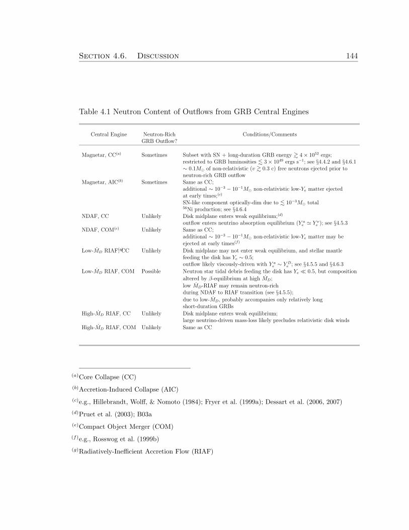
Section 4.6. Discussion 144
Table 4.1 Neutron Content of Outflows from GRB Central Engines
Central Engine Neutron-Rich Conditions/CommentsGRB Outflow?
Magnetar, CC(a) Sometimes Subset with SN + long-duration GRB energy & 4× 1052 ergs;restricted to GRB luminosities . 3× 1049 ergs s−1; see §4.4.2 and §4.6.1∼ 0.1M¯ of non-relativistic (v & 0.3 c) free neutrons ejected prior toneutron-rich GRB outflow
Magnetar, AIC(b) Sometimes Same as CC;additional ∼ 10−3 − 10−1M¯ non-relativistic low-Ye matter ejectedat early times;(c)
SN-like component optically-dim due to . 10−3M¯ total56Ni production; see §4.6.4
NDAF, CC Unlikely Disk midplane enters weak equilibrium;(d)
outflow enters neutrino absorption equilibrium (Y ae ' Y ν
e ); see §4.5.3NDAF, COM(e) Unlikely Same as CC;
additional ∼ 10−3 − 10−1M¯ non-relativistic low-Ye matter may beejected at early times(f)
Low-MD RIAF(g), CC Unlikely Disk midplane may not enter weak equilibrium, and stellar mantlefeeding the disk has Ye ∼ 0.5;outflow likely viscously-driven with Y a
e ∼ Y De ; see §4.5.5 and §4.6.3
Low-MD RIAF, COM Possible Neutron star tidal debris feeding the disk has Ye ¿ 0.5, but composition
altered by β-equilibrium at high MD;
low MD-RIAF may remain neutron-richduring NDAF to RIAF transition (see §4.5.5);
due to low-MD, probably accompanies only relatively longshort-duration GRBs
High-MD RIAF, CC Unlikely Disk midplane enters weak equilibrium;large neutrino-driven mass-loss likely precludes relativistic disk winds
High-MD RIAF, COM Unlikely Same as CC
(a)Core Collapse (CC)
(b)Accretion-Induced Collapse (AIC)
(c)e.g., Hillebrandt, Wolff, & Nomoto (1984); Fryer et al. (1999a); Dessart et al. (2006, 2007)
(d)Pruet et al. (2003); B03a
(e)Compact Object Merger (COM)
(f)e.g., Rosswog et al. (1999b)
(g)Radiatively-Inefficient Accretion Flow (RIAF)
Section 4.6. Discussion 145
circumstances. In agreement with previous works (e.g., Daigne & Mochkovitch
2002; Levinson 2006), we find that outflows with σ & 100 are possible from the
innermost radii of NDAFs around rapidly rotating black holes (a ≈ 1), despite the
minimum neutrino-driven mass-loss rate (eq. [4.24]). The significantly larger M re-
quired for a large neutron excess, however, precludes neutron-rich NDAF outflows
from attaining σ & 1−10 for significant accretion powers (eq. [4.26]). Furthermore,
because modest entropy, magnetocentrifugally-driven winds only possess free nu-
clei over a relatively limited range of radii, cross-field diffusion is ineffective at
polluting otherwise neutron-poor axial jets with free neutrons from adjacent, more
heavily baryon-loaded winds (see §4.5.4).
Although we find that neutron-rich winds from NDAFs are unlikely, several
caveats should be discussed. Pruet et al. (2004) suggest that “bubbles” of neutron-
rich material may escape the disk via chaotically-heated buoyant magnetic fila-
ments, a picture similar to some models for GRBs (Narayan et al. 1992; Katz
1997; Kluzniak & Ruderman 1998). Although this possibility cannot be ruled out,
current thin disk simulations do not find significant energy deposition in low den-
sity, coronal regions (e.g., Hirose, Krolik, & Stone 2006), and whether such low-Ye
bubbles can remain neutron-rich despite the pair-capture deneutronization that
accompanies such chaotic heating is unclear. If the Blandford-Znajek mechanism
or ν−ν annihilation above the disk’s rotation axis powers the GRB outflow instead
of a disk wind, the base of the GRB-producing jet may be effectively baryon-free
because the field lines would then thread the black hole’s event horizon instead
the disk midplane; what ultimately sets the wind’s baryon-loading in this case is
unclear. Our calculations show that neutrino-heated disk winds will form a modest
entropy “sheath” around such a baryon-free jet. If, however, the wind encasing the
jet possesses a much higher entropy (e.g., Pruet et al. 2001), cross-field neutron
diffusion is more effective (Levinson & Eichler 2003; McKinney 2005b) and may
result in asymptotically neutron-rich polar outflow. Furthermore, even if the out-
flow’s field lines don’t thread the disk, it is in principle possible that some form of
chaotic mass-loading may pollute the baryon-poor base of the jet with matter from
the neutron-rich disk midplane. We note, however, that current simulations find
Section 4.6. Discussion 146
very little matter entraining the jet from the disk, thus requiring implementation
of a numerical density floor along the polar axis (e.g., Proga & Begelman 2003;
Proga et al. 2003).
4.6.3 Thick Disks
Although NDAFs exist over a range of accretion rates that are relevant to both
long and short-duration GRBs, GRB-producing outflows can also be powered by
the accretion of matter that is not efficiently neutrino-cooled. Such geometrically-
thick, radiatively-inefficient accretion flows (RIAFs) exist for both MD < Mign
(“low-MD RIAFs”), for which the density is too low for efficient neutrino cooling
near Risco, and for MD À Mign (“high-MD RIAFs”), for which matter advects
into the black hole faster than it cools (e.g., Di Matteo, Perna, & Narayan 2002).
High MD RIAFs, while possibly relevant to “prompt” collapsars (MacFadyen &
Woosley 1999), are probably most relevant to compact object mergers given their
smaller expected disk radii and shorter accretion timescales. Low-MD RIAFs are
relevant to both the late stages of collapsars and compact binary mergers.
Like NDAFs, high-MD RIAFs enter β-equilibrium before accreting and, al-
though they are not as neutron-rich as NDAFs, they also typically have Y De ¿ 0.5
(e.g., Surman & McLaughlin 2004; Lee et al. 2005, hereafter L05). High-MD RI-
AFs are confined to radii in the disk smaller than the “trapping” radius Rt, the
point interior to which matter has insufficient time to cool before accreting; Rt
exists outside Risco for mass accretion rates greater than Mt ≈ 9(2)α1/30.1M¯ s−1
for a = 0(0.95) and M = 3M¯ (CB07). Although radiatively-inefficient on the
whole, disks with MD > Mt still release a substantial neutrino luminosity because
Mt is large and accretion is still efficiently cooled for radii larger than Rt; in-
deed, for steady-state accretion, Di Matteo, Perna, & Narayan (2002) find that as
MD increases beyond Mt, Lν saturates to a value ∼ 1053 ergs s−1. This substan-
tial neutrino luminosity will drive significant neutrino-heated mass-loss, thereby
severely limiting the asymptotic Lorentz factor Γ of any outflow driven from the
RIAF’s surface. Using the simulations of L05 (their Fig. 6), we estimate that the
Section 4.6. Discussion 147
neutrinosphere temperature of a high-MD RIAF near Rt is roughly Tν ∼ 3 MeV
(corresponding to a mean neutrino energy 〈εν〉 ∼ 10 MeV); thus, from equation
(4.19) we estimate that the minimum, neutrino-driven mass-loss rate from the
innermost radii of high-MD RIAFs is Mth ≈ 10−3 − 10−2M¯ s−1. For a wind
driven from the surface of a high-MD RIAF to reach Γ & 100 would thus require
an MHD luminosity E & 1053 − 1054 ergs s−1, which is comparable to the entire
accretion power for MD ∼ Mt ∼ 1 − 10M¯ s−1 and is substantially larger than
the outflow powers typically inferred from short-duration GRBs (e.g., Bloom et
al. 2005). GRB-producing outflows, whether neutron-rich or not, are thus unlikely
to originate from disk winds produced by high-MD RIAFs.
Unlike NDAFs and high-MD RIAFs, low-MD RIAFs may not enter weak equi-
librium on an accretion timescale (eq. [4.28]); thus, the electron fraction in a low-
MD thick disk’s midplane can remain approximately equal to that of the material
used to form the disk initially. Because of the low neutrino luminosity and positive
Bernoulli parameters of low-MD RIAFs, viscous heating likely dominates neutrino
heating in outflows driven from low-MD thick disks, thereby making deneutron-
ization by neutrinos unlikely. Although nondegenerate pair-captures may drive
Ye → 0.5 depending on the precise viscous energy deposition profile in the wind,
this possibility is less likely than for NDAF outflows because weak equilibrium is
already slow in the disk midplane and because the accretion and outflow advec-
tion rates for thick disks are comparable. Furthermore, if acceleration from the
midplane is enhanced due to magnetocentrifugal slinging, pair-capture deneutron-
ization would be further suppressed. Thus, outflows driven from low-MD RIAFs
probably retain the electron fraction of the disk’s original composition. As a result,
outflows driven at late times from collapsars, which are fed from the progenitor
star’s relatively neutron-poor envelope (e.g., Ye ' 0.5 for a purely He composi-
tion), probably do not possess a significant neutron excess. In this case, significant
56Ni could be produced in the disk’s outflow, powering a bright SN (MacFadyen
& Woosley 1999).
Although disks formed from compact object mergers are usually initially
neutron-rich, they are compact and nearly all of the matter goes through an NDAF
Section 4.6. Discussion 148
phase in which weak equilibrium modifies the initial composition of the disk; their
composition at late times therefore depends on how they transition from an NDAF
to a low-MD thick disk. Depending on α, the size of the disk, and the mass of
the black hole, the composition of the thick disk immediately following the NDAF
to low-MD RIAF transition at tign can be either neutron-rich or proton-rich (see
eq. [4.29]). Although by no means assured, neutron-rich GRBs outflows may thus
be possible from thick disks in both collapsars immediately following tign (espe-
cially if the variability imposed by the NDAF-thick disk transition actually causes
the GRB; Giannios 2007) and in short-duration GRBs from compact object merg-
ers. In either case, neutron-rich GRB outflows should be restricted to events with
accretion power (and thus maximum GRB luminosity) less than Lν,ign (eq. [4.7]).
4.6.4 Non-Relativistic Neutron-Rich Winds
Optical Transients
Relativistic, GRB-producing outflows from proto-magnetars and hyper-
accreting disks are possible under specialized circumstances, but non-relativistic
winds are also likely to be present, probably occur in a wider variety of progenitors,
and probably carry more total energy. The composition of such non-relativistic
winds may also lead to an observable signature, most directly via radiation from
ejecta that is reheated by the decay of radioactive elements in the wind. One
possibility in the case of magnetar birth is that the heavily mass-loaded wind that
emerges at early times (carrying a total mass up to∼ 0.01−0.1M¯ for a millisecond
rotator; Dessart et al. 2007; see Fig. 2.10) could produce a bright SN-like event.
However, by combining the mass-loss rate that accompanies a significant neutron
excess (eq. [4.18]) with the fiducial PNS cooling evolution Lν(t) given in equation
(4.8), we find that the total PNS mass-loss capable of being processed into 56Ni
under NSE (which requires no significant neutron excess; Hartmann, Woosley, &
El Eid 1985) cannot exceed MmaxNi ∼
∫ τKH
1 sMthφndt ∼ 10−3M¯, much too small to
contribute appreciably to an optical light curve powered by 56Ni, and subsequent
Section 4.6. Discussion 149
56Co, decay (e.g., see Kulkarni 2005, Fig. 7).13
The modest optical luminosity associated with the decay of a mass ∼ MmaxNi
of Ni is consistent with the rather stringent upper limits on the SN component
accompanying some short-duration GRBs (e.g., GRB050509B; Hjorth et al. 2005);
this supports the viability of a model in which short-duration GRBs are powered by
the rapid spin-down of a magnetized, rapidly rotating magnetar, formed following
the accretion-induced collapse (AIC) of a white dwarf (Usov 1992) or resulting
from the merger of a double neutron star binary (a “super-pulsar”; Rosswog et
al. 2003). It is less clear how much of the substantial mass-loss driven from the
accretion disk formed during the merger of two compact objects will be processed
into 56Ni. Quantifying this will require additional work.
Even if little mass is ejected with Y ae & 0.5 (capable of producing 56Ni), both
proto-magnetars and hyper-accreting disks could in principle produce detectable
transients due to the presence of neutron-rich non-relativistic outflows. For exam-
ple, a proto-magnetar that is born rotating sufficiently rapidly to produce late-time,
relativistic neutron-rich matter must also eject a total massMn & 0.1M¯ in slower
(v & 0.3 c) free neutrons at earlier times. The detectability of such neutron-rich
non-relativistic outflows is, however, uncertain. Any neutrons that ultimately re-
main free in the wind will β-decay into protons on a timescale τβ ≈ 900 s at a
radius & 1013 cm; thus, one observable manifestation of neutron-rich outflow may
be Li-Paczynski mini-SN (“Macronovae”) powered by the thermal energy released
by this decay (≈ 6× 1049(Mn/0.1M¯) ergs), which may be detectable on hour-day
timescales following the birth of the central object (Li & Paczynski 1998; Kulkarni
2005).
13Enhanced Ni production is still possible in the core collapse context via early energization of asuccessful SN shock due to rapid spin-down (TCQ04). A proto-magnetar’s spin-down luminosityis substantially enhanced over the vacuum-dipole rate at early times following the launch of theSN shock by the excess magnetic flux opened by neutrino-heated, centrifugally-driven mass-loss(B06). In this case, the enhanced Ni yield is produced by additional shock heating of the stellarprogenitor, not directly in the wind itself.
Section 4.6. Discussion 150
r-process Nucleosynthesis
Rather than leaving free neutrons, the decompression of slowly moving, mod-
est entropy, and moderately neutron-rich (0.1 . Y ae . 0.4) matter is more likely to
produce anomalous neutron-rich isotopes (e.g., 62Ni, 66Zn, 68Zn, 87Rb, 88Sr; Hart-
mann, Woosley, & El Eid 1985), and in some cases may be capable of producing
r-process elements (e.g., Freiburghaus et al. 1999). Thus, as a final application of
our calculations, we briefly consider the possibility of r-process element synthesis
in proto-magnetar and NDAF winds. Given their intrinsic neutron-rich nature,
outflows from neutron star formation have long been considered one of the most
promising r-process sites (Woosley & Hoffman 1992; Meyer et al. 1992); how-
ever, the conditions necessary for a successful third-peak r-process have not been
realized in detailed studies of non-rotating, non-magnetized PNS winds (QW96;
Otsuki et al. 2000; Sumiyoshi et al. 2000; Wanajo et al. 2001; T01). In Chapter
2 we studied the effects of magnetic fields and rotation on the r-process in PNS
winds for P & Pn and constant Ye; although we did not find solutions with a suc-
cessful third-peak r-process (based on the criteria of Hoffman, Woosley, & Qian
1997, hereafter HWQ97), we did not consider the additional benefits of low Y ae
caused by very rapid rotation (P < Pn).
Even accounting for the possibility of low Ye discussed in this paper, we find
that all of the NDAF and most of the proto-magnetar wind solutions we have
considered still fail to meet the criteria for third-peak r-process of HWQ97, mainly
because the beneficial effects of low Ye are counteracted by the detrimental effects
that the accompanying rapid advection has on the wind’s asymptotic entropy Sa.14
One possibility is that energy deposition by acoustic or MHD waves could raise
the asymptotic entropy of low-Ye winds (Suzuki & Nagataki 2005; Chapter 2). In
14By the arguments given in §4.2, for a PNS wind to remain neutron-rich the thermal energydeposited in the wind per baryon cannot exceed the neutrinosphere’s mean neutrino energy 〈εν〉.Thus, because most heating occurs near the PNS surface (at a temperature ≈ 0.7Tν ; QW96,eq. [47]), the entropy added to a neutron-rich wind cannot exceed ∆S ∼ 〈εν〉/0.7Tν ≈ 5 kBbaryon−1 (compare Sa and Y a
e in Tables 4.3 and 4.4), which is substantially less than that de-posited in non-magnetized, non-rotating PNS winds ∆S ≈ GMmn/0.7TνRν ≈ 70(Lνe,51/8)
−1/4
kB baryon−1 (QW96; T01).
Section 4.6. Discussion 151
addition, despite their extremely low entropy, some of the most rapidly rotating
and highly magnetized proto-magnetar solutions that we have calculated (e.g., the
Bν = 1016 G and Ω = 9000 Hz solution shown in Figure 4.3) do eclipse the third-
peak r-process threshold of HWQ97. This occurs because r-process synthesis of
nuclei with mean mass A (typically ∼ 195 for the third peak) by neutron captures
on seed nuclei with mean proton number Z (typically ∼ 30 − 40) is possible for
Y ae . Z/A ≈ 0.15 − 0.20, even in outflows with vanishingly small Sa (see the
discussion in Wheeler et al. 1998). The dynamical timescales for our very low Y ae
solutions are, however, much shorter than those considered by HWQ97 and several
commonly made assumptions become suspect for such rapidly expanding outflows
(Meyer 2002); thus, detailed nucleosynthesis calculations, which include all of the
relevant rate equations, need to be completed in the regime of low Sa, low Y ae , and
very rapid outflow before r-process success is assured.
The very rapid rotation and strong magnetic fields associated with the suc-
cessful r-process winds that we find are extreme and will not accompany most
core-collapse SNe; the substantial amount of neutron-rich material (& 0.1M¯)
ejected by such a proto-magnetar, however, means that just a few very rapidly
rotating proto-magnetar births of this kind per Myr would noticeably affect the
Galactic r-process abundance (Qian 2000). Conversely, if the r-process yield from
events like this do not resemble the observed abundances, the number of sub-
millisecond magnetar births in our Galaxy can be strongly constrained; similar
constraints can be placed on the incidence of the accretion-induced collapse (AIC)
of a white dwarf, which produces a similar yield of low Ye material (e.g., Woosley
& Baron 1992; Fryer et al. 1999a; Dessart et al. 2006, 2007).
Acknowledgements
We thank Niccolo Bucciantini and Jon Arons for helpful discussions. We thank
Wen-xin Chen and Andrei Beloborodov for making their accretion disk solu-
tions available to us. EQ and BDM were supported in part by NASA grant
NNG05GO22H, the David and Lucile Packard Foundation, and a NASA GSRP
Section 4.6. Discussion 152
Fellowship to BDM. Wind profiles are available upon request from BDM.
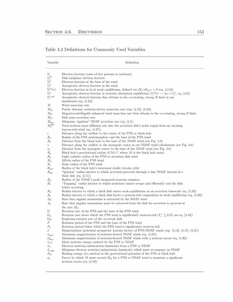
Section 4.6. Discussion 153
Table 4.2 Definitions for Commonly Used Variables
Variable Definition
Ye Electron fraction (ratio of free protons to nucleons)Y De Disk midplane electron fractionY 0e Electron fraction at the base of the windY ae Asymptotic electron fraction in the windY eqe (r) Electron fraction in local weak equilibrium, defined via dYe/dt|Y eq
e= 0 (eq. [4.14])
Y νe Asymptotic electron fraction in neutrino absorption equilibrium (Y eq
e (r →∞) = Y νe ; eq. [4.6])
Y a,sate Asymptotic electron fraction that obtains in the co-rotating, strong B limit in our
simulations (eq. [4.16])
M Wind mass-loss rate
Mth Purely thermal, neutrino-driven mass-loss rate (eqs. [4.19], [4.24])
Mcf Magnetocentrifugally-enhanced wind mass-loss rate that obtains in the co-rotating, strong B limit
MD Disk mass accretion rate
Mign Minimum “ignition” NDAF accretion rate (eq. [4.1])
Mdiffn Total neutron mass diffusion rate into the accretion disk’s polar region from an encasing
baryon-rich wind (eq. [4.27]).r Distance along the outflow to the center of the PNS or black holeRν Radius of the PNS neutrinosphere and the base of the PNS windR0 Distance from the black hole to the base of the NDAF wind (see Fig. 4.6)s Distance along the outflow to the monopole center in our NDAF wind calculations (see Fig. 4.6)s0 Distance from the monopole center to the base of the NDAF wind (see Fig. 4.6)Rg Black hole’s gravitational radius (GM/c2, where M is the black hole mass)RL Light cylinder radius of the PNS or accretion disk windRA Alfven radius of the PNS windRs Sonic radius of the PNS windRisco Radius of the black hole’s innermost stable circular orbitRign “Ignition” radius interior to which accretion proceeds through a thin NDAF instead of a
thick disk (eq. [4.11])Rp Radius of the NDAF’s peak integrated neutrino emissionRt “Trapping” radius interior to which neutrinos cannot escape and efficiently cool the disk
before accretingRβ Radius interior to which a thick disk enters weak equilibrium on an accretion timescale (eq. [4.28])Rn Radius interior to which a thick disk favors a neutron-rich composition in weak equilibrium (eq. [4.29])
JW Rate that angular momentum is extracted by the NDAF wind
JD Rate that angular momentum must be extracted from the disk for accretion to proceed at
the rate MD
Ω Rotation rate of the PNS and the base of the PNS windΩn Rotation rate above which the PNS wind is significantly neutron-rich (Y a
e . 0.25; see eq. [4.16])ΩK Keplerian rotation rate of the accretion diskP Rotation period of the PNS and the base of the PNS windPn Rotation period below which the PNS wind is significantly neutron-richσ Magnetization (potential asymptotic Lorentz factor) of PNS/NDAF winds (eqs. [4.13], [4.15], [4.21])σmax Maximum magnetization of neutrino-heated NDAF winds (eq. [4.25])σnmax Maximum magnetization of neutrino-heated NDAF winds with a neutron excess (eq. [4.26])〈εν〉 Mean neutrino energy emitted by the PNS or NDAFLν Electron neutrino/antineutrino luminosity from a PNS or NDAFLν,ign Minimum electron neutrino/antineutrino luminosity which must accompany an NDAFEB Binding energy of a nucleon in the gravitational potential of the PNS or black hole
φn Factor by which M must exceed Mth for a PNS or NDAF wind to maintain a significantneutron excess (eq. [4.18])
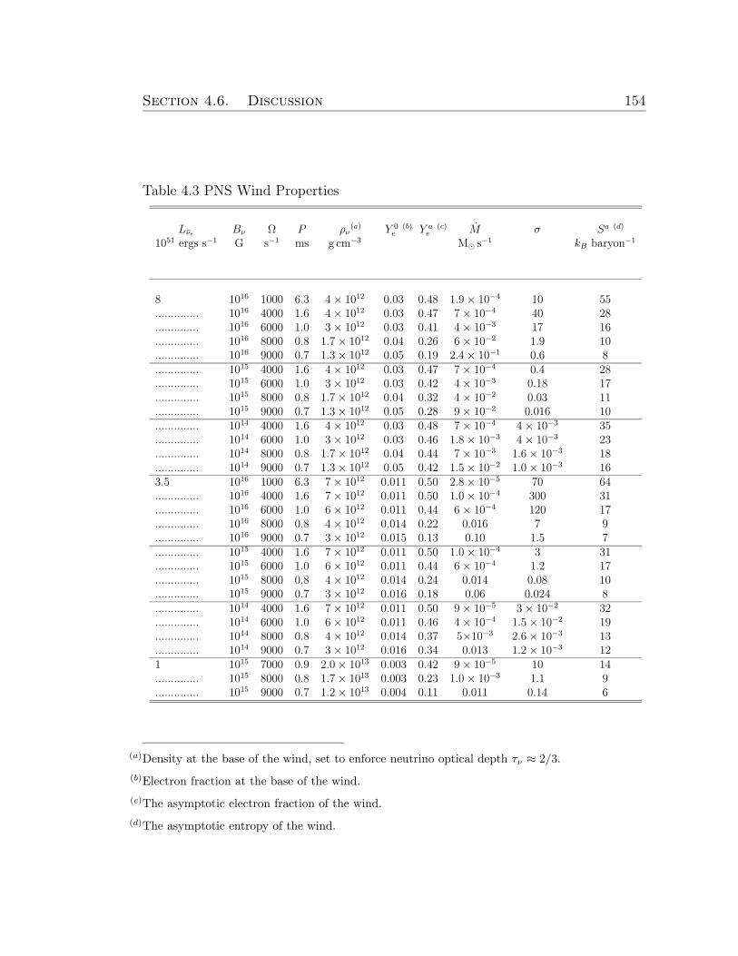
Section 4.6. Discussion 154
Table 4.3 PNS Wind Properties
Lνe Bν Ω P ρν(a) Y 0
e(b) Y a
e(c) M σ Sa (d)
1051 ergs s−1 G s−1 ms g cm−3 M¯ s−1 kB baryon−1
8 1016 1000 6.3 4× 10¹² 0.03 0.48 1.9× 10⁻⁴ 10 55.............. 1016 4000 1.6 4× 10¹² 0.03 0.47 7× 10⁻⁴ 40 28.............. 1016 6000 1.0 3× 10¹² 0.03 0.41 4× 10⁻³ 17 16.............. 1016 8000 0.8 1.7× 10¹² 0.04 0.26 6× 10⁻² 1.9 10.............. 1016 9000 0.7 1.3× 10¹² 0.05 0.19 2.4× 10⁻¹ 0.6 8.............. 1015 4000 1.6 4× 10¹² 0.03 0.47 7× 10⁻⁴ 0.4 28.............. 1015 6000 1.0 3× 10¹² 0.03 0.42 4× 10⁻³ 0.18 17.............. 1015 8000 0.8 1.7× 10¹² 0.04 0.32 4× 10⁻² 0.03 11.............. 1015 9000 0.7 1.3× 10¹² 0.05 0.28 9× 10⁻² 0.016 10.............. 1014 4000 1.6 4× 10¹² 0.03 0.48 7× 10⁻⁴ 4× 10⁻³ 35.............. 1014 6000 1.0 3× 10¹² 0.03 0.46 1.8× 10⁻³ 4× 10⁻³ 23.............. 1014 8000 0.8 1.7× 10¹² 0.04 0.44 7× 10⁻³ 1.6× 10⁻³ 18.............. 1014 9000 0.7 1.3× 10¹² 0.05 0.42 1.5× 10⁻² 1.0× 10⁻³ 163.5 1016 1000 6.3 7× 10¹² 0.011 0.50 2.8× 10⁻⁵ 70 64.............. 1016 4000 1.6 7× 10¹² 0.011 0.50 1.0× 10⁻⁴ 300 31.............. 1016 6000 1.0 6× 10¹² 0.011 0.44 6× 10⁻⁴ 120 17.............. 1016 8000 0.8 4× 10¹² 0.014 0.22 0.016 7 9.............. 1016 9000 0.7 3× 10¹² 0.015 0.13 0.10 1.5 7.............. 1015 4000 1.6 7× 10¹² 0.011 0.50 1.0× 10⁻⁴ 3 31.............. 1015 6000 1.0 6× 10¹² 0.011 0.44 6× 10⁻⁴ 1.2 17.............. 1015 8000 0.8 4× 10¹² 0.014 0.24 0.014 0.08 10.............. 1015 9000 0.7 3× 10¹² 0.016 0.18 0.06 0.024 8.............. 1014 4000 1.6 7× 10¹² 0.011 0.50 9× 10⁻⁵ 3× 10⁻² 32.............. 1014 6000 1.0 6× 10¹² 0.011 0.46 4× 10⁻⁴ 1.5× 10⁻² 19.............. 1014 8000 0.8 4× 10¹² 0.014 0.37 5×10⁻³ 2.6× 10⁻³ 13.............. 1014 9000 0.7 3× 10¹² 0.016 0.34 0.013 1.2× 10⁻³ 121 1015 7000 0.9 2.0× 10¹³ 0.003 0.42 9× 10⁻⁵ 10 14.............. 1015 8000 0.8 1.7× 10¹³ 0.003 0.23 1.0× 10⁻³ 1.1 9.............. 1015 9000 0.7 1.2× 10¹³ 0.004 0.11 0.011 0.14 6
(a)Density at the base of the wind, set to enforce neutrino optical depth τν ≈ 2/3.
(b)Electron fraction at the base of the wind.
(c)The asymptotic electron fraction of the wind.
(d)The asymptotic entropy of the wind.
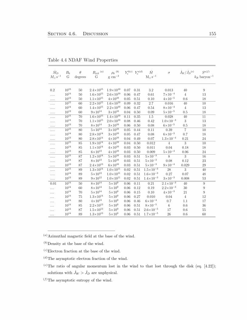
Section 4.6. Discussion 155
Table 4.4 NDAF Wind Properties
MD B0 θ Bφ,0(a) ρ0
(b) Y 0e(c) Y a
e(d) M σ JW/JD
(e) Sa(f)
M¯ s−1 G degrees G g cm−3 M¯ s
−1 kB baryon−1
0.2 1015 50 2.4×10¹⁵ 1.9×10¹⁰ 0.07 0.31 3.2 0.013 40 9..... 1014 50 1.6×10¹⁵ 2.6×10¹⁰ 0.06 0.47 0.61 7×10⁻⁴ 4 13..... 1013 50 1.1×10¹⁵ 4×10¹⁰ 0.05 0.51 0.10 4×10⁻⁵ 0.6 18..... 1015 60 2.2×10¹⁵ 1.6×10¹⁰ 0.09 0.32 2.7 0.016 40 10..... 1014 60 1.4×10¹⁵ 2.2×10¹⁰ 0.06 0.47 0.54 8×10⁻⁴ 4 13..... 1013 60 9×10¹⁴ 3×10¹⁰ 0.04 0.50 0.09 5×10⁻⁵ 0.5 18..... 1015 70 1.6×10¹⁵ 1.4×10¹⁰ 0.11 0.35 1.5 0.028 40 11..... 1014 70 1.1×10¹⁵ 2.0×10¹⁰ 0.08 0.46 0.42 1.0×10⁻³ 3 13..... 1013 70 8×10¹⁴ 3×10¹⁰ 0.06 0.50 0.08 6×10⁻⁵ 0.5 18..... 1015 80 5×10¹⁴ 3×10¹⁰ 0.05 0.44 0.11 0.39 7 10..... 1014 80 2.8×10¹⁴ 3×10¹⁰ 0.05 0.47 0.08 6×10⁻³ 0.7 18..... 1013 80 2.8×10¹⁴ 4×10¹⁰ 0.04 0.49 0.07 1.3×10⁻⁴ 0.21 24..... 1015 85 1.9×10¹⁴ 4×10¹⁰ 0.04 0.50 0.012 4 3 10..... 1014 85 1.1×10¹⁴ 4×10¹⁰ 0.03 0.50 0.011 0.04 0.18 18..... 1013 85 6×10¹³ 4×10¹⁰ 0.03 0.50 0.009 5×10⁻⁴ 0.06 24..... 1015 87 1.2×10¹⁴ 5×10¹⁰ 0.03 0.51 5×10⁻³ 8 3 16..... 1014 87 8×10¹³ 5×10¹⁰ 0.03 0.51 5×10⁻³ 0.08 0.12 23..... 1013 87 2.4×10¹³ 6×10¹⁰ 0.03 0.51 5×10⁻³ 9×10⁻⁴ 0.029 29..... 1015 89 1.3×10¹⁴ 1.0×10¹¹ 0.02 0.51 1.5×10⁻³ 28 3 40..... 1014 89 5×10¹³ 1.0×10¹¹ 0.02 0.51 1.6×10⁻³ 0.27 0.07 48..... 1013 89 9×10¹² 1.0×10¹¹ 0.02 0.51 1.4×10⁻³ 3×10⁻³ 0.008 53
0.01 1014 50 8×10¹⁴ 5×10⁹ 0.06 0.11 0.21 2.1×10⁻³ 40 9.... 1014 60 8×10¹⁴ 5×10⁹ 0.06 0.12 0.19 2.2×10⁻³ 30 9.... 1014 70 5×10¹⁴ 5×10⁹ 0.06 0.15 0.10 4×10⁻³ 21 9.... 1014 75 1.3×10¹⁴ 5×10⁹ 0.06 0.27 0.010 0.04 4 12.... 1014 80 4×10¹³ 5×10⁹ 0.06 0.46 6×10⁻⁴ 0.7 1.1 17.... 1014 85 2.2×10¹³ 5×10⁹ 0.06 0.51 8×10⁻⁵ 6 0.6 36.... 1014 87 1.5×10¹³ 5×10⁹ 0.06 0.51 2.6×10⁻⁵ 17 0.6 55.... 1014 89 1.3×10¹³ 5×10⁹ 0.06 0.51 1.7×10⁻⁵ 26 0.6 60
(a)Azimuthal magnetic field at the base of the wind.
(b)Density at the base of the wind.
(c)Electron fraction at the base of the wind.
(d)The asymptotic electron fraction of the wind.
(e)The ratio of angular momentum lost in the wind to that lost through the disk (eq. [4.22]);
solutions with JW > JD are unphysical.
(f)The asymptotic entropy of the wind.
156
Chapter 5
Time-Dependent Models of
Accretion Disks Formed from
Compact Object Mergers
B. D. Metzger, A. L. Piro, E. Quataert (2008), MNRAS, 390, 781-797.1
Abstract
We present time-dependent models of the remnant accretion disks created
during compact object mergers, focusing on the energy available from accretion
at late times and the composition of the disk and its outflows. We calculate the
dynamics near the outer edge of the disk, which contains the majority of the disk’s
mass and determines the accretion rate onto the central black hole. This treatment
allows us to follow the evolution over much longer timescales (100 s or longer) than
current hydrodynamic simulations. At late times the disk becomes advective and
its properties asymptote to self-similar solutions with an accretion rate Md ∝ t−4/3
(neglecting outflows). This late-time accretion can in principle provide sufficient
energy to power the late-time activity observed by Swift from some short-duration
gamma-ray bursts. However, because outflows during the advective phase unbind
1Copyright 2008. Royal Astronomical Society. All rights reserved.
Section 5.1. Introduction 157
the majority of the remaining mass, it is difficult for the remnant disk alone to
produce significant accretion power well beyond the onset of the advective phase.
Unless the viscosity is quite low (α . 10−3), this occurs before the start of observed
flaring at ∼ 30 s; continued mass inflow at late times thus appears required to
explain the late-time activity from short-duration gamma-ray bursts. We show
that the composition of the disk freezes-out when the disk is relatively neutron
rich (electron fraction Ye ' 0.3). Roughly 10−2M¯ of this neutron-rich material is
ejected by winds at late times. During earlier, neutrino-cooled phases of accretion,
neutrino irradiation of the disk produces a wind with Ye ' 0.5, which synthesizes
at most ∼ 10−3M¯ of 56Ni. We highlight what conditions are favorable for 56Ni
production and predict, in the best cases, optical and infrared transients peaking
∼ 0.5 − 2 days after the burst, with fluxes a factor of ∼ 10 below the current
observational limits.
5.1 Introduction
The most popular model for the creation of short-duration gamma-ray bursts
(GRBs) is either binary neutron star (NS/NS) or black hole-neutron star (BH/NS)
coalescence (Paczynski 1986, 1991; Eichler et al. 1989; Narayan et al. 1992). Sup-
port for the merger hypothesis comes from their durations of . 2 s, observations
of well-localized short GRBs in galaxies without strong star formation (Berger et
al. 2005; Gehrels et al. 2005; Hjorth et al. 2005), and the lack of a detectable co-
incident supernovae (Hjorth et al. 2005; Bloom et al. 2006; Soderberg et al. 2006;
Ferrero et al. 2007), as is found in the case of long (& 2 s) GRBs (Galama et
al. 1998; Hjorth et al. 2003; Stanek et al. 2003).
Previous theoretical studies of the merger process have focused on one of two
stages. The first is the dynamical portion in which the less massive companion
is tidally disrupted by the more massive BH (Lee & Kluzniak 1995, 1998, 1999;
Kluzniak & Lee 1998; Janka et al. 1999; Rosswog et al. 2004) or NS (Ruffert et
al. 1996; Ruffert & Janka 1999; Oechslin & Janka 2006). The details of whether a
dynamical instability (Rasio & Shapiro 1994; Lai et al. 1994) or Roche lobe overflow
Section 5.1. Introduction 158
occurs depends on the mass ratio and the nuclear equation of state (Bildsten &
Cutler 1992; Uryu & Eriguchi 1999).
Nevertheless, generally ∼ 0.01 − 0.1M¯ of material remains in a remnant
disk following the dynamical stage. The accretion of this material onto the cen-
tral object gives rise to the second, disk portion of the merger. The energetics
and timescale of the accretion phase are reasonably consistent with observations
of short GRBs, as was shown by models of steady-state, azimuthally symmetric,
vertically averaged disks (Popham et al. 1999; Narayan et al. 2001; Kohri & Mi-
neshige 2002; Di Matteo et al. 2002; Chen & Beloborodov 2007). More recently,
these disks have been modeled with time-dependent calculations in 1D (Janiuk et
al. 2004), 2D (Lee et al. 2004, 2005b), and 3D (Setiawan et al. 2004, 2006). The
typical time interval that present multi-dimensional calculations can simulate is
on the order of the burst duration or less (∼ 1− 2 s for 2D and ∼ 50 ms for 3D).
Recent observations of short GRBs by Swift, however, indicate continued ac-
tivity from the central engine on much longer timescales. X-ray flares with du-
rations of ∼ 100 s after a delay of ∼ 30 s have been seen from several bursts
(Barthelmy et al. 2005; Villasenor et al. 2005; Campana et al. 2006; La Parola
et al. 2006). Stacked lightcurves of many bursts indicate continued activity on a
similar timescale (Lazzati et al. 2001; Montanari et al. 2005). In one extreme case,
GRB 050724 displayed an X-ray flare 12 hours post-burst. This flaring activity
has been attributed to a number of different sources, including fragmentation of a
rapidly rotating core (King et al. 2005), magnetic regulation of the accretion flow
(Proga & Zhang 2006), fragmentation of the accretion disk (Perna et al. 2005; al-
though this explanation may have difficulty reproducing the observed timescales,
Piro & Pfahl 2007), differential rotation in a post-merger millisecond pulsar (Dai
et al. 2007), and an infalling tidal tail of material stripped from the disrupted NS
(Lee & Ramirez-Ruiz 2007; Rosswog 2007).
In order to determine whether the late-time activity from short GRBs is con-
sistent with a compact merger origin, the disk evolution should be followed for
timescales much longer than the initial viscous time. With this aim, we perform
time-dependent calculations modeling the disk as an annulus that contains the
Section 5.2. Initial Conditions 159
majority of the mass. This simplification allows us to study the disk evolution for
arbitrarily long timescales, and to readily determine important properties such as
the disk’s composition and when it becomes advective. We are also able to survey
much of the parameter space of initial disk mass and angular momentum. In §5.2
we discuss the initial conditions for disks formed from compact object mergers.
This is followed by §5.3, in which we summarize the main assumptions of our ring
model. In §5.4 we present the results of our calculations and summarize the main
properties of the models. We then calculate outflows from our disk solutions in
§5.5. We investigate the composition of the outflows and argue that they generally
consist of neutron-rich isotopes, but can produce 56Ni in some circumstances. The
presence or lack of an optical transient from short GRBs therefore provides an
important constraint on progenitor models. We conclude in §5.6 with a discussion
of our results. In Appendix A we summarize the Green’s function solution to the
viscous spreading of a ring, which is important for connecting our ring model to
the true extended disk geometry. In Appendix B we present analytic self-similar
solutions that reproduce many of the features of our numerical solutions.
5.2 Initial Conditions
The dynamical phase of NS/NS or BH/NS mergers has been studied exten-
sively using a number of different numerical techniques and methods for including
general relativity (GR). Here we summarize some of the most relevant features for
our study (for a more detailed review, see Lee & Ramirez-Ruiz 2007).
When the lighter companion NS is first tidally disrupted, a debris disk is
formed within only a few dynamical timescales. The initial disk mass, Md,0, is
generally larger for more asymmetric mass ratios (i.e., small q, where q is the ratio
of the lighter to the heavier binary component). For example, Shibata & Taniguichi
(2006) find that for a NS/NS merger with q = 0.7 that Md,0 = 0.03 M¯, but for
q = 0.9 the disk is much less massive with Md,0 = 10−3 M¯. Another trend
is that including strong gravity gives less massive remnant disks. The BH spin is
also important, with larger spin favoring disk formation (Rasio et al. 2005) and the
Section 5.2. Initial Conditions 160
production of a tidal tail. These have masses of ' 0.01−0.05M¯ and may provide
prolonged mass inflow (Lee & Ramirez-Ruiz 2007), but for simplicity this will be
ignored here. Taken together, these simulations generally findMd,0 ' 0.01−0.3M¯,
with the disk containing a substantial fraction of the angular momentum of the
disrupted companion.
In the standard picture of NS-NS mergers, the resulting hypermassive NS col-
lapses to a BH shortly following the merger. However, simulations show that when
(and if) collapse actually occurs depends on the mass of the central NS and its abil-
ity to transport angular momentum to the surrounding disk (Shibata et al. 2005;
Shibata & Taniguchi 2006; Shibata et al. 2006). In fact, if the NS remains sup-
ported by differential rotaton for several seconds (Baumgarte et al. 2000; Morrison
et al. 2004; Duez et al. 2004, 2006) or loses sufficient mass via a centrifugally-driven
outflow (e.g., Thompson et al. 2004; Dessart et al. 2008a), the NS itself may power
the GRB (e.g., Price & Rosswog 2006). In this paper we assume that the central
object promptly collapses to a BH; our model, however, would be reasonably ap-
plicable for the case of a central NS as well, the primary difference being that the
significant neutrino flux from the newly-formed NS and from the boundary layer
between the disk and the NS could modify the composition and thermal properties
of the disk.
We present some characteristic numbers to motivate our choice of initial con-
ditions. Consider a binary with massesM and m (M > m), where the latter is the
NS (with radius R) that is tidally disrupted. The disruption radius, at, is estimated
to be (Kopal 1959, adding Fishbone’s 1973 10% strong-gravity correction)
at ' 2.4R
(
M +m
m
)1/3
. (5.1)
The characteristic orbital period at this radius is
Pt ' 23.4
(
R3
Gm
)1/2
' 2× 10⁻³m−1/21.4 R
3/26 s, (5.2)
where m1.4 = m/1.4 M¯ and R6 = R/106 cm, with an orbital angular momentum
of
Jt ' (G(M +m)at)1/2m ' 6× 1049(1/q + 1)2/3m
3/21.4R
1/26 ergs s, (5.3)
Section 5.3. Physics of the Expanding Ring Model 161
where q = m/M . The disrupted NS also contains spin angular momentum. This is
negligible since the NS is not strongly affected by tidal coupling (Bildsten & Cutler
1992). Even a rapidly rotating NS (' 5 ms) has an associated angular momentum
of merely ∼ 1048 ergs s.
Once disrupted, a considerable fraction of the NS is either lost from the system
or immediately swallowed by the BH. The remaining material forms a thick torus
surrounding the central BH. Its associated viscous timescale can be estimated by
assuming that the majority of the mass of the torus lies at a single radius, rd,0.
Taking the angular momentum of the disk to be Jd ' (GMrd,0)1/2Md,0, we estimate
rd,0 ' 3× 10⁷M−13 M−2
0.1
(
J492
)2
cm, (5.4)
where M3 = M/3 M¯, M0.1 = Md,0/0.1 M¯, and J49 = Jd/1049 ergs s. For a disk
with half-thickness H, the viscous timescale is
tvisc,0 = α−1(rdH
)2(
r3dGM
)1/2
' 6× 10⁻²α−10.1M−1/23 r
3/27
(
H
0.5rd
)−2
s, (5.5)
where α = 0.1α0.1 is the standard dimensionless viscosity (Shakura & Sunyaev
1973), r7 = rd,0/107 cm, and we have scaled to an initial ratio of H/rd = 0.5, con-
sistent with our numerical solutions. The initial viscous time tvisc,0 is roughly the
time at which the central BH begins accreting in earnest. The strong dependence
of tvisc,0 on disk mass and radius demonstrates that the initial evolution of the disk
is sensitive to the outcome of the dynamical phase of the merger. But as we will
show, the late time evolution is much less sensitive to initial conditions and is well
described by self-similar solutions.
5.3 Physics of the Expanding Ring Model
Given these initial conditions, one would like to know how the disk then
evolves. Modeling the entire disk requires resolving timescales over ∼ 4− 6 orders
of magnitude. This makes it expensive to carry out simulations for long periods of
time. We consider instead a simplified model that captures most of the features of
Section 5.3. Physics of the Expanding Ring Model 162
interest. At any given time, t, the disk can be broken into three regions depending
on the local viscous time, tvisc, which increases with radius, roughly as tvisc ∼ r3/2.
At small radii, tvisc < t, and the disk comes into steady-state. This is the region
most often modeled in previous studies (Popham et al. 1999; Narayan et al. 2001;
Kohri & Mineshige 2002; Di Matteo et al. 2002; Chen & Beloborodov 2007).
The radii where tvisc ∼ t contain the majority of the disk’s mass and angular
momentum. Therefore, this region determines the viscous evolution of the rest of
the disk, including the mass accretion rate that is fed to the interior steady-state
region. Motivated by this fact, we focus on this radius and model the disk as a
ring. Exterior to this point is a third region where tvisc > t, but this contains a
small amount of mass and is negligible for the viscous evolution.
5.3.1 Dynamical Equations
Our ring model treats the disk as a single annulus that is evolved forward
in time. In this picture, the properties of the ring, such as its surface density Σ
and temperature T , are representative of the location where Σr2 peaks. The main
drawback of this method is that the material in the disk is in fact distributed
spatially in radius. Thus, although the mass of the disk in the vicinity of rd is
' πΣr2d, the total mass of the disk (integrated over all radii) is Md = AπΣr2d,
where A is a factor of order unity that accounts for the distinction between the
total mass of the disk and the mass of the material near rd. Similarly, we write
the total angular momentum of the disk as Jd = B(GMrd)1/2πr2dΣ. At early times
the constants A and B depend on the initial conditions of how matter is spatially
distributed; however, at times much greater than the initial viscous time (given
by eq. [5.5]), material initially concentrated at a given radius becomes spread out
in a manner determined by the viscosity. As described in detail in Appendix A,
we choose the constants A and B by setting the solution of our simplified ring
model at late times equal to the Green’s function solution for a spreading ring
with a viscosity ν ∝ r1/2 (as is appropriate for the radiatively inefficient disk at
Section 5.3. Physics of the Expanding Ring Model 163
late-times). This fixes A = 3.62 and B = 3.24.2 Conveniently A/B ' 1, so that it
is a good approximation to take Jd ' (GMrd)1/2Md.
The time evolution of the disk is determined by the conservation equations.
Conservation of mass isd
dt
(
AπΣr2d)
= −Md, (5.6)
where Md is in general the total mass-loss rate, which could include both accretion
and a wind (for now we ignore the effects of a wind). Conservation of angular
momentum isd
dt
[
B(GMrd)1/2πΣr2d
]
= −J , (5.7)
where J is the angular momentum-loss rate. Equations (5.6) and (5.7) provide
two coupled equations that can be solved for the dependent variables rd and Σ.
The accretion rate must depend on the characteristic mass and viscous timescale
of the ring, so we use
Md = fMd/tvisc, (5.8)
where tvisc = r2d/ν and ν is the viscosity. The factor f is set like A and B to match
the exact solution of a spreading ring with ν ∝ r1/2 (Appendix A), which gives
f = 1.6.3 Requiring a no-torque boundary condition at a radius r∗, we take
f = 1.6/[1− (r∗/rd)1/2]. (5.9)
In contrast, a steady-state disk obeys Md = 3πνΣ (ignoring the no-torque condi-
tion), which instead gives f = 3/A ' 0.83.
For the viscosity, we use an α-prescription,
ν = αcsH, (5.10)
where cs = (P/ρ)1/2 is the isothermal sound speed. The equation of state in-
cludes contributions from radiation pressure, gas pressure, relativistic degeneracy
pressure, and neutrino pressure as in Di Matteo et al. (2002).
2In fact, when the total angular momentum is conserved, the viscous evolution is independentof A/B as long as A/B is nearly constant with time.
3Although we set tvisc = r2/ν, any prefactors that could go into this prescription would justbe absorbed into a re-definition of f .
Section 5.3. Physics of the Expanding Ring Model 164
5.3.2 Energetics
For the energy equation, we take
qvisc = q−ν + qadv, (5.11)
where qvisc is the viscous heating, q−ν is the neutrino cooling (using the prescriptions
given by Di Matteo et al. 2002, which includes neutrino optical-depth effects), qadv
is the advective heat flux, and all q values correspond to half the disk thickness.
For a disk rotating at the Keplerian frequency Ω = (GM/r3d)1/2,
qvisc =9
8νΩ2Σ =
9
8fA
GMMd
πr3d
[
1−
(
r∗rd
)1/2]
, (5.12)
where the prefactor 9/(8fA) ' 0.2 is different from the steady-state value of
3/8. The advective term, qadv, is set as in Di Matteo et al. (2002), with the only
difference being that the radial velocity is the expansion rate of the ring’s radius
Vr =drddt
=2M
AπrdΣ, (5.13)
where we have taken J = 0.
Fusion to α-particles produces heating in addition to qvisc, with
qnucl = 6.8× 1028ρ10dXα
dtH, (5.14)
where all quantities are expressed in cgs units, ρ10 = ρ/1010 g cm−3 and Xα is
the mass fraction of α-particles. Note that in our case qnucl > 0 since α-particles
are synthesized as the disk expands (in contrast to studies that follow cooling
from photodisintegration as material moves inward). In our calculations we do not
include qnucl in solving equation (5.11) because we were not able to find reasonable
solutions when doing so (for reasons explained in §5.4.1).
5.3.3 Composition
An advantage of the ring model is that other properties of the disk, such as
its composition, can be cast into differential equations and integrated along with
Section 5.3. Physics of the Expanding Ring Model 165
equations (5.6) and (5.7). Since the neutron content of the disk is particularly
important for determining the properties of the disk’s outflows, we evolve the
electron fraction Ye using
dYedt
= −Yere−p + (1− Ye)re+n, (5.15)
where Ye = Xp/(Xn +Xp), Xp and Xn are the proton and neutron mass fraction,
respectively, and re−p and re+n are the electron and positron capture rates, respec-
tively (Beloborodov 2003a). We have neglected the effect of neutrino absorptions
on the evolution of Ye in equation (5.15). Although absorptions are important at
early times when the disk is optically thick, we are primarily concerned with the
late-time value of Ye, which does not depend sensitively on the neutrino irradiation
(see §5.4.2).
As the disk evolves, the protons and neutrons eventually burn to form α-
particles. At these times the disk is sufficiently cold that the positron and electron
capture rates are negligible (i.e, 1/re−p À tvisc) and Ye has frozen-out. This fixes
the difference between the free neutron and proton mass fractions
Xn −Xp = 1− 2Ye. (5.16)
Since the rates for reactions that synthesize and destroy α-particles are all fast
in comparison to the viscous time, we determine the composition using nuclear
statistical equilibrium (NSE) between protons, neutron, and α-particles. This is
expressed by the Saha relation (Shapiro & Teukolsky 1983)
X2pX
2n = 1.57× 10⁴ Xαρ
−310 T
9/210 exp
(
−32.81
T10
)
. (5.17)
NSE is a good assumption because the disk temperature is generally & 0.5 MeV
(see Fig. 5.2), except at very late times or for very low disk masses (e.g., theMd,0 =
0.03M¯ case, for which we do not calculate the nuclear composition anyways). By
combining equations (5.16) and (5.17) with mass conservation, Xp+Xn+Xα = 1,
we solve for all of the mass fractions at a given ρ, T , and Ye.
Section 5.4. Time-Evolving Solutions 166
5.4 Time-Evolving Solutions
We next present the results of integrating equations (5.6), (5.7), and (5.15)
forward in time. For simplicity, we typically assume that J = 0. A convenient
property of our formalism is the ease with which these complications can be in-
cluded (for example, we consider the effects of winds at the end of §4.1). The disk
properties are determined by the initial conditions Md,0, Jd, and Ye,0, and by the
viscosity α. For the majority of our study we set the initial Ye,0 = 0.1, which is
characteristic of the inner neutron star crust (Haensel & Zdunik 1990a,b; Pethick &
Ravenhall 1995). An additional important parameter is r∗, which is set by the spin
of the central BH. In most of our calculations we take r∗ ' 2.3rg ' 1.02× 106 cm,
corresponding to the innermost stable circular orbit of a 3 M¯ BH with spin
a ' 0.9; when calculating the properties of disk outflows in §5.5, however, we also
consider the case of a nonrotating (a = 0) BH. We consider the general evolution
of the disk in §5.4.1, and then focus on the composition in §5.4.2.
5.4.1 Disk Evolution and Energetics
At any given time, a ring model is in one of three phases: (1) early-time,
optically thick to neutrinos and advectively dominated, (2) mid-time, optically
thin to neutrinos and geometrically thin, and (3) late-time, radiatively-inefficient
accretion flow (RIAF).4 This is analogous to the different regions of steady-state,
hyper-accreting accretion disks (see, e.g., Chen & Beloborodov 2007), but now
the transitions occur with time instead of radius. The phases that a certain ring
model samples during the course of its viscous expansion depends on tvisc,0. A
more compact disk (a shorter tvisc,0) will exhibit all three phases, while larger disks
may only exhibit phases (2) and (3), or even just (3).
We present a number of figures that are helpful in understanding these three
phases and how they are affected by changing Md,0. Figure 5.1 shows the radius
4An optically thick, geometrically thin stage occurs between stages (1) and (2); however, thisphase is brief and is not dynamically very different from phase (2), so we do not consider itseparately in our discussion.
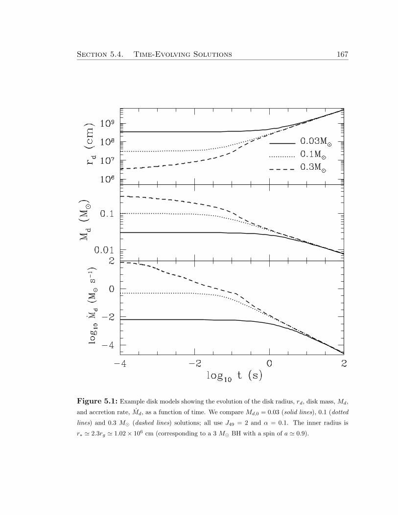
Section 5.4. Time-Evolving Solutions 167
Figure 5.1: Example disk models showing the evolution of the disk radius, rd, disk mass, Md,
and accretion rate, Md, as a function of time. We compare Md,0 = 0.03 (solid lines), 0.1 (dotted
lines) and 0.3 M¯ (dashed lines) solutions; all use J49 = 2 and α = 0.1. The inner radius is
r∗ ' 2.3rg ' 1.02× 106 cm (corresponding to a 3 M¯ BH with a spin of a ' 0.9).
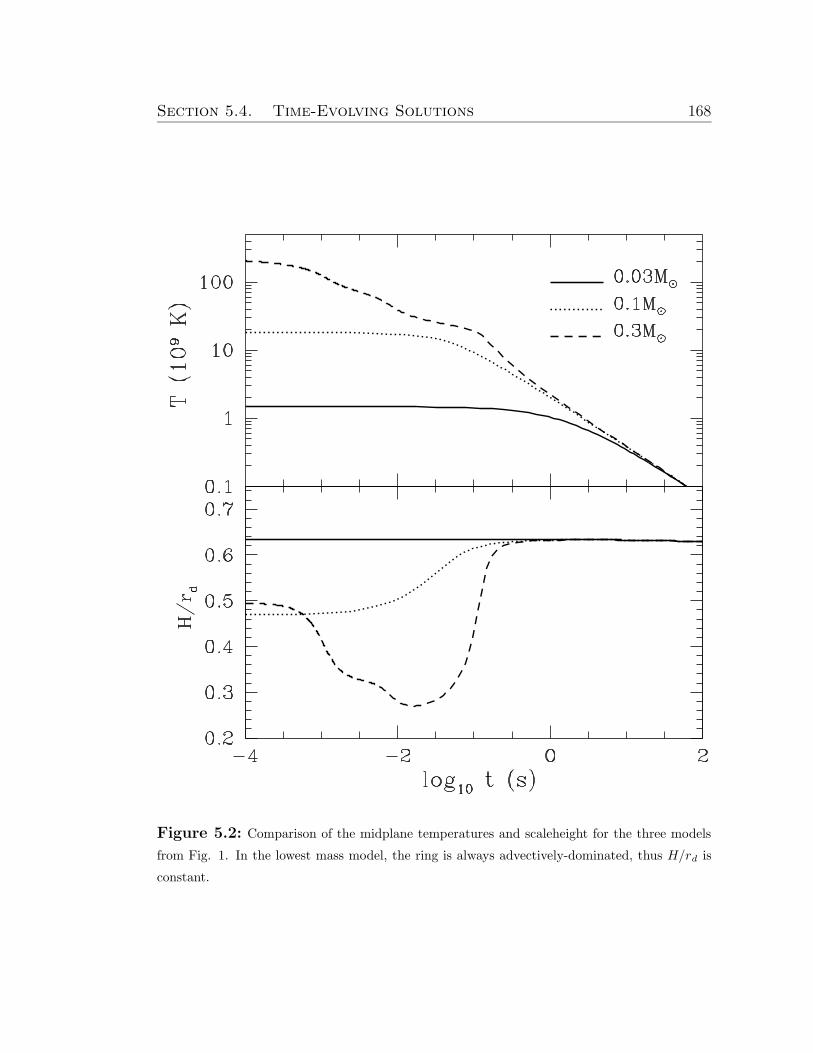
Section 5.4. Time-Evolving Solutions 168
Figure 5.2: Comparison of the midplane temperatures and scaleheight for the three models
from Fig. 1. In the lowest mass model, the ring is always advectively-dominated, thus H/rd is
constant.
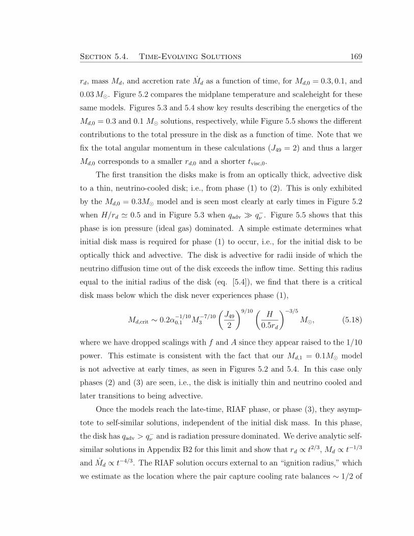
Section 5.4. Time-Evolving Solutions 169
rd, mass Md, and accretion rate Md as a function of time, for Md,0 = 0.3, 0.1, and
0.03M¯. Figure 5.2 compares the midplane temperature and scaleheight for these
same models. Figures 5.3 and 5.4 show key results describing the energetics of the
Md,0 = 0.3 and 0.1 M¯ solutions, respectively, while Figure 5.5 shows the different
contributions to the total pressure in the disk as a function of time. Note that we
fix the total angular momentum in these calculations (J49 = 2) and thus a larger
Md,0 corresponds to a smaller rd,0 and a shorter tvisc,0.
The first transition the disks make is from an optically thick, advective disk
to a thin, neutrino-cooled disk; i.e., from phase (1) to (2). This is only exhibited
by the Md,0 = 0.3M¯ model and is seen most clearly at early times in Figure 5.2
when H/rd ' 0.5 and in Figure 5.3 when qadv À q−ν . Figure 5.5 shows that this
phase is ion pressure (ideal gas) dominated. A simple estimate determines what
initial disk mass is required for phase (1) to occur, i.e., for the initial disk to be
optically thick and advective. The disk is advective for radii inside of which the
neutrino diffusion time out of the disk exceeds the inflow time. Setting this radius
equal to the initial radius of the disk (eq. [5.4]), we find that there is a critical
disk mass below which the disk never experiences phase (1),
Md,crit ∼ 0.2α−1/100.1 M
−7/103
(
J492
)9/10(H
0.5rd
)−3/5
M¯, (5.18)
where we have dropped scalings with f and A since they appear raised to the 1/10
power. This estimate is consistent with the fact that our Md,1 = 0.1M¯ model
is not advective at early times, as seen in Figures 5.2 and 5.4. In this case only
phases (2) and (3) are seen, i.e., the disk is initially thin and neutrino cooled and
later transitions to being advective.
Once the models reach the late-time, RIAF phase, or phase (3), they asymp-
tote to self-similar solutions, independent of the initial disk mass. In this phase,
the disk has qadv > q−ν and is radiation pressure dominated. We derive analytic self-
similar solutions in Appendix B2 for this limit and show that rd ∝ t2/3, Md ∝ t−1/3
and Md ∝ t−4/3. The RIAF solution occurs external to an “ignition radius,” which
we estimate as the location where the pair capture cooling rate balances ∼ 1/2 of
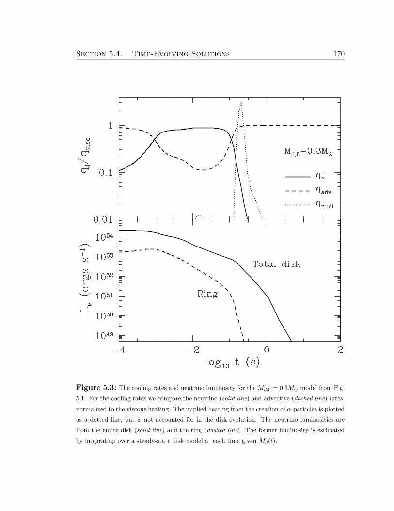
Section 5.4. Time-Evolving Solutions 170
Figure 5.3: The cooling rates and neutrino luminosity for the Md,0 = 0.3M¯ model from Fig.
5.1. For the cooling rates we compare the neutrino (solid line) and advective (dashed line) rates,
normalized to the viscous heating. The implied heating from the creation of α-particles is plotted
as a dotted line, but is not accounted for in the disk evolution. The neutrino luminosities are
from the entire disk (solid line) and the ring (dashed line). The former luminosity is estimated
by integrating over a steady-state disk model at each time given Md(t).
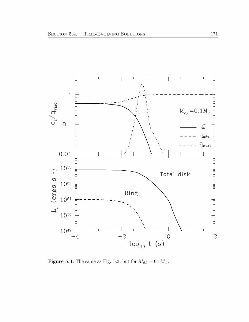
Section 5.4. Time-Evolving Solutions 171
Figure 5.4: The same as Fig. 5.3, but for Md,0 = 0.1M¯.
Section 5.4. Time-Evolving Solutions 172
the viscous heating for a thick disk,
rign ' 3× 10⁷α−20.1M−3/53
(
H/rd0.4
)−14/5(
Md
0.1M¯s−1
)6/5
cm, (5.19)
where we have scaled H/rd to ≈ 0.4, a value appropriate for the transition between
the thin and thick disk regimes. We combine this with the analytic results for rd(t)
and Md(t) in the RIAF limit (eqs. [5.48] and [5.47])5 to estimate the time when
the disk transitions to being thick, which yields
tthick ∼ 0.1α−23/170.1 M
−13/173
(
J492
)9/17
s. (5.20)
Equation (5.20) is only applicable if the disk is thin at early times. For sufficiently
small initial disk masses, less than
Md,thick ∼ 0.1α2/170.1 M
−7/173
(
J492
)14/17
M¯, (5.21)
this is no longer true, and the disk is always a RIAF at its outer radius.
Figures 5.3 and 5.4 show that at approximately the same time as the disk tran-
sitions from being thin to thick, protons and neutrons are fused to He. Although
the nuclear heating rate qnuc is shown in Figures 5.3 and 5.4, this heating was not
included in our time-dependent calculations so that we could obtain solutions at
late times. The nuclear heating rate is sufficiently large, i.e, qnucl & qvisc, that the
disk is not able to accommodate this added energy (it is already thick with H ' r
due to viscous heating alone). This probably implies that the burning contributes
to driving a powerful wind (as described by Lee & Ramirez-Ruiz 2007).
However, such a wind already begins at this time by virtue of the disk being
advective (as discussed in §5.5.2). In Appendix B3, we present analytic self-similar
solutions for advective disks with mass loss and show that this significant mass-
loss causes Md and Md to decline much more rapidly with time than is shown in
Figure 5.1. This is shown explicitly in Figure 5.6, where we present disk models
calculated using the mass and angular momentum-loss prescriptions described in
5We use these solutions rather than the thin-disk ones because the numerical results followthese more closely (Fig. 5.15).
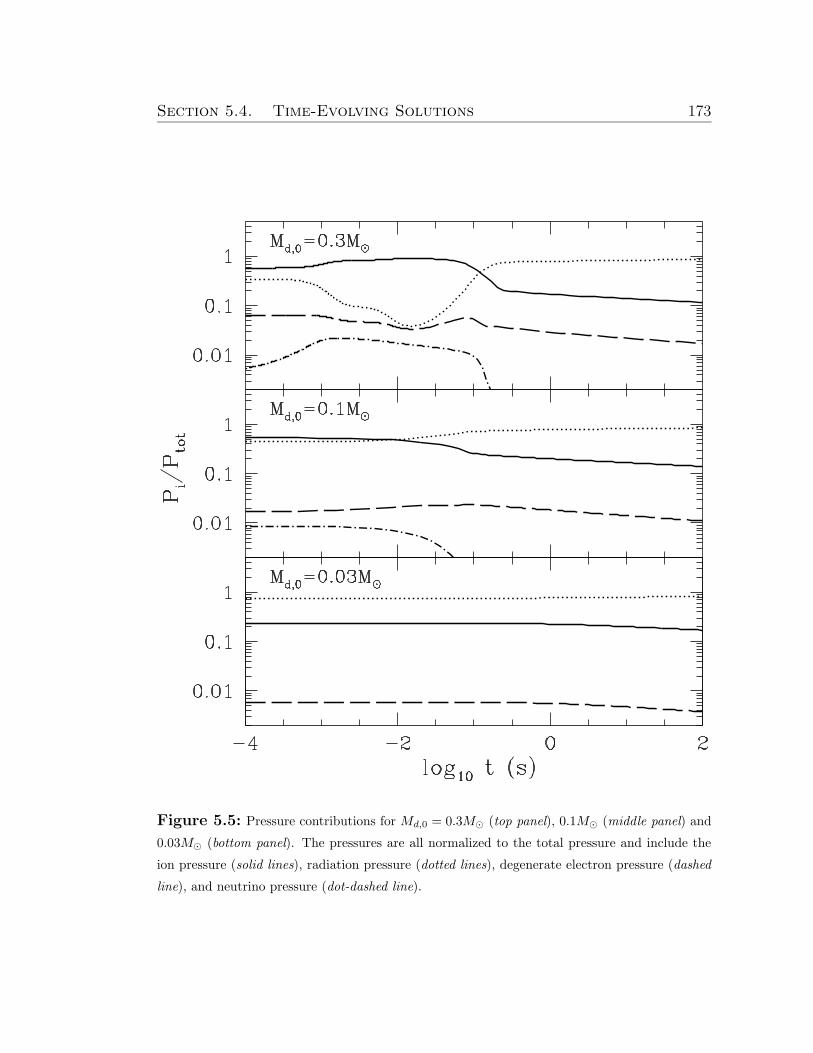
Section 5.4. Time-Evolving Solutions 173
Figure 5.5: Pressure contributions for Md,0 = 0.3M¯ (top panel), 0.1M¯ (middle panel) and
0.03M¯ (bottom panel). The pressures are all normalized to the total pressure and include the
ion pressure (solid lines), radiation pressure (dotted lines), degenerate electron pressure (dashed
line), and neutrino pressure (dot-dashed line).
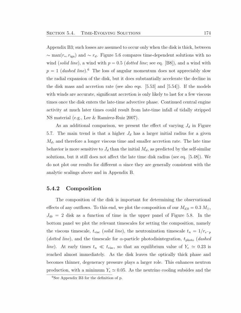
Section 5.4. Time-Evolving Solutions 174
Appendix B3; such losses are assumed to occur only when the disk is thick, between
∼ max(r∗, rign) and ∼ rd. Figure 5.6 compares time-dependent solutions with no
wind (solid line), a wind with p = 0.5 (dotted line; see eq. [B8]), and a wind with
p = 1 (dashed line).6 The loss of angular momentum does not appreciably slow
the radial expansion of the disk, but it does substantially accelerate the decline in
the disk mass and accretion rate (see also eqs. [5.53] and [5.54]). If the models
with winds are accurate, significant accretion is only likely to last for a few viscous
times once the disk enters the late-time advective phase. Continued central engine
activity at much later times could result from late-time infall of tidally stripped
NS material (e.g., Lee & Ramirez-Ruiz 2007).
As an additional comparison, we present the effect of varying Jd in Figure
5.7. The main trend is that a higher Jd has a larger initial radius for a given
Md, and therefore a longer viscous time and smaller accretion rate. The late time
behavior is more sensitive to Jd than the initialMd, as predicted by the self-similar
solutions, but it still does not affect the late time disk radius (see eq. [5.48]). We
do not plot our results for different α since they are generally consistent with the
analytic scalings above and in Appendix B.
5.4.2 Composition
The composition of the disk is important for determining the observational
effects of any outflows. To this end, we plot the composition of ourMd,0 = 0.3M¯,
J49 = 2 disk as a function of time in the upper panel of Figure 5.8. In the
bottom panel we plot the relevant timescales for setting the composition, namely
the viscous timescale, tvisc (solid line), the neutronization timescale tn = 1/re−p
(dotted line), and the timescale for α-particle photodisintegration, tphoto (dashed
line). At early times tn ¿ tvisc, so that an equilibrium value of Ye ' 0.23 is
reached almost immediately. As the disk leaves the optically thick phase and
becomes thinner, degeneracy pressure plays a larger role. This enhances neutron
production, with a minimum Ye ' 0.05. As the neutrino cooling subsides and the
6See Appendix B3 for the definition of p.
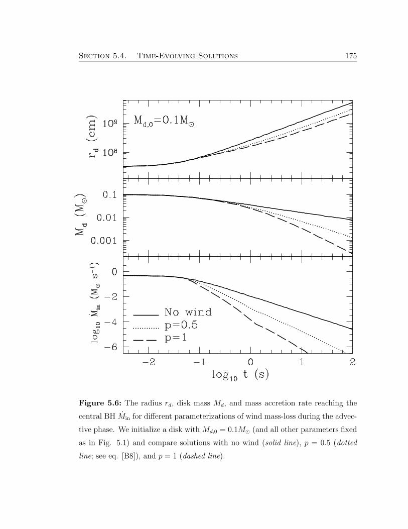
Section 5.4. Time-Evolving Solutions 175
Figure 5.6: The radius rd, disk mass Md, and mass accretion rate reaching the
central BH Min for different parameterizations of wind mass-loss during the advec-
tive phase. We initialize a disk with Md,0 = 0.1M¯ (and all other parameters fixed
as in Fig. 5.1) and compare solutions with no wind (solid line), p = 0.5 (dotted
line; see eq. [B8]), and p = 1 (dashed line).
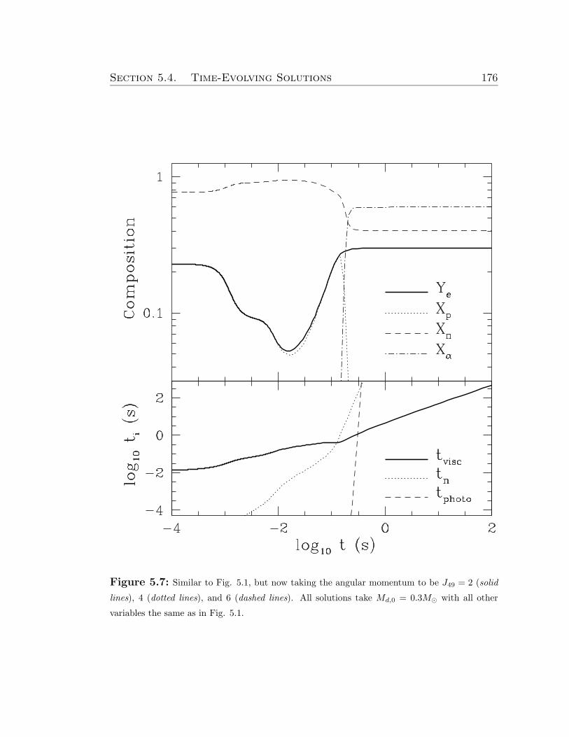
Section 5.4. Time-Evolving Solutions 176
Figure 5.7: Similar to Fig. 5.1, but now taking the angular momentum to be J49 = 2 (solid
lines), 4 (dotted lines), and 6 (dashed lines). All solutions take Md,0 = 0.3M¯ with all other
variables the same as in Fig. 5.1.
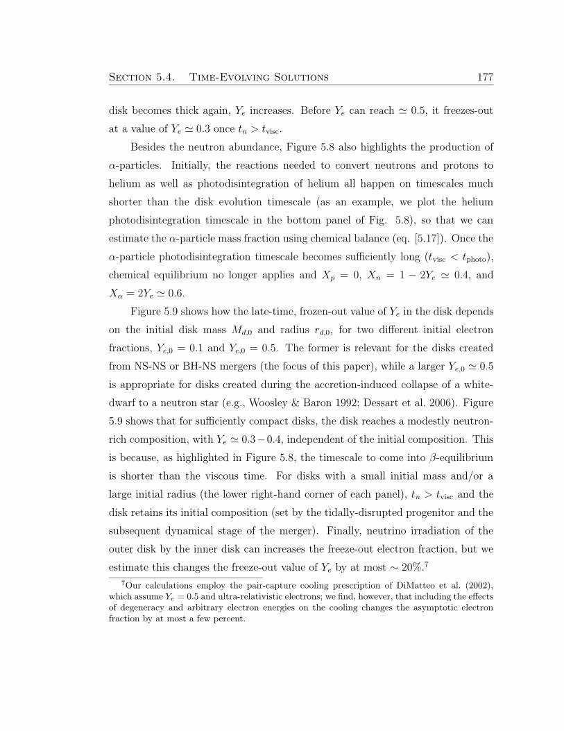
Section 5.4. Time-Evolving Solutions 177
disk becomes thick again, Ye increases. Before Ye can reach ' 0.5, it freezes-out
at a value of Ye ' 0.3 once tn > tvisc.
Besides the neutron abundance, Figure 5.8 also highlights the production of
α-particles. Initially, the reactions needed to convert neutrons and protons to
helium as well as photodisintegration of helium all happen on timescales much
shorter than the disk evolution timescale (as an example, we plot the helium
photodisintegration timescale in the bottom panel of Fig. 5.8), so that we can
estimate the α-particle mass fraction using chemical balance (eq. [5.17]). Once the
α-particle photodisintegration timescale becomes sufficiently long (tvisc < tphoto),
chemical equilibrium no longer applies and Xp = 0, Xn = 1 − 2Ye ' 0.4, and
Xα = 2Ye ' 0.6.
Figure 5.9 shows how the late-time, frozen-out value of Ye in the disk depends
on the initial disk mass Md,0 and radius rd,0, for two different initial electron
fractions, Ye,0 = 0.1 and Ye,0 = 0.5. The former is relevant for the disks created
from NS-NS or BH-NS mergers (the focus of this paper), while a larger Ye,0 ' 0.5
is appropriate for disks created during the accretion-induced collapse of a white-
dwarf to a neutron star (e.g., Woosley & Baron 1992; Dessart et al. 2006). Figure
5.9 shows that for sufficiently compact disks, the disk reaches a modestly neutron-
rich composition, with Ye ' 0.3−0.4, independent of the initial composition. This
is because, as highlighted in Figure 5.8, the timescale to come into β-equilibrium
is shorter than the viscous time. For disks with a small initial mass and/or a
large initial radius (the lower right-hand corner of each panel), tn > tvisc and the
disk retains its initial composition (set by the tidally-disrupted progenitor and the
subsequent dynamical stage of the merger). Finally, neutrino irradiation of the
outer disk by the inner disk can increases the freeze-out electron fraction, but we
estimate this changes the freeze-out value of Ye by at most ∼ 20%.7
7Our calculations employ the pair-capture cooling prescription of DiMatteo et al. (2002),which assume Ye = 0.5 and ultra-relativistic electrons; we find, however, that including the effectsof degeneracy and arbitrary electron energies on the cooling changes the asymptotic electronfraction by at most a few percent.
Section 5.4. Time-Evolving Solutions 178
Figure 5.8: The composition and important reaction timescales as a function of time, for the
Md,0 = 0.3M¯ model from Fig. 5.1. In the top panel we plot the electron fraction, Ye and the
mass fraction of protons, neutrons, and α-particles (see inset key). In the bottom panel we show
the viscous time, tvisc (thick, solid line), the neutronization time, tn = 1/re−p (dotted line), and
the α-particle photodisintegration time, tphoto (dashed line).
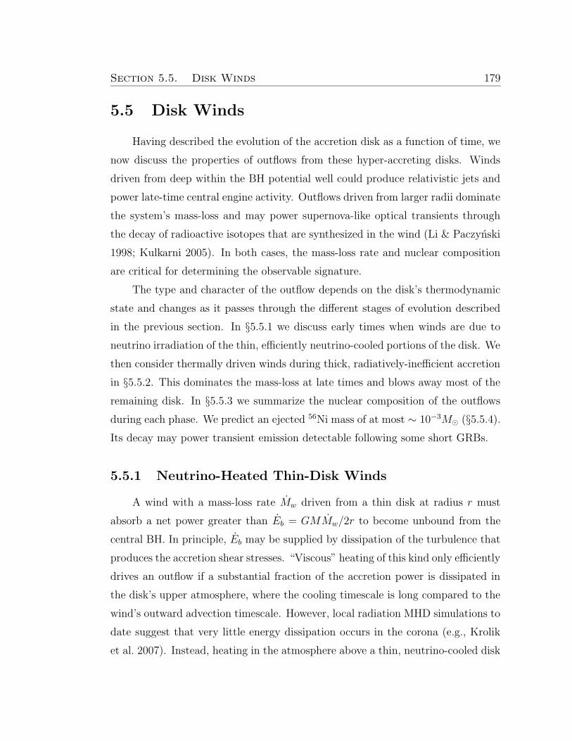
Section 5.5. Disk Winds 179
5.5 Disk Winds
Having described the evolution of the accretion disk as a function of time, we
now discuss the properties of outflows from these hyper-accreting disks. Winds
driven from deep within the BH potential well could produce relativistic jets and
power late-time central engine activity. Outflows driven from larger radii dominate
the system’s mass-loss and may power supernova-like optical transients through
the decay of radioactive isotopes that are synthesized in the wind (Li & Paczynski
1998; Kulkarni 2005). In both cases, the mass-loss rate and nuclear composition
are critical for determining the observable signature.
The type and character of the outflow depends on the disk’s thermodynamic
state and changes as it passes through the different stages of evolution described
in the previous section. In §5.5.1 we discuss early times when winds are due to
neutrino irradiation of the thin, efficiently neutrino-cooled portions of the disk. We
then consider thermally driven winds during thick, radiatively-inefficient accretion
in §5.5.2. This dominates the mass-loss at late times and blows away most of the
remaining disk. In §5.5.3 we summarize the nuclear composition of the outflows
during each phase. We predict an ejected 56Ni mass of at most ∼ 10−3M¯ (§5.5.4).
Its decay may power transient emission detectable following some short GRBs.
5.5.1 Neutrino-Heated Thin-Disk Winds
A wind with a mass-loss rate Mw driven from a thin disk at radius r must
absorb a net power greater than Eb = GMMw/2r to become unbound from the
central BH. In principle, Eb may be supplied by dissipation of the turbulence that
produces the accretion shear stresses. “Viscous” heating of this kind only efficiently
drives an outflow if a substantial fraction of the accretion power is dissipated in
the disk’s upper atmosphere, where the cooling timescale is long compared to the
wind’s outward advection timescale. However, local radiation MHD simulations to
date suggest that very little energy dissipation occurs in the corona (e.g., Krolik
et al. 2007). Instead, heating in the atmosphere above a thin, neutrino-cooled disk
Section 5.5. Disk Winds 180
Figure 5.9: Contours of late-time electron fraction in the expanding disk as a function of
initial disk mass Md,0 and radius rd,0, for two different initial compositions. Relatively compact
disks come into β-equilibrium and reach an electron fraction independent of the initial Ye, while
low mass, more extended disks retain their initial composition. Figure 5.8 shows the evolution
of Ye with time for one particular disk solution.
Section 5.5. Disk Winds 181
is likely dominated by neutrino irradiation. We therefore focus on the neutrino-
driven mass-loss rate, which sets a minimum Mw, and which can be reliably esti-
mated. Neutrino-driven outflows from hyper-accreting disks have also been studied
in Chapter 4 and by Daigne & Mochkovitch (2002), Levinson (2006), and Barzilay
& Levinson (2008); Dessart et al. (2008b) calculate the neutrino-driven mass-loss
from the central NS following a NS-NS merger under the assumption that collapse
to a BH is not prompt.
The neutrino-driven mass-loss rate is calculated by equating Eb to the to-
tal neutrino heating rate in the disk’s atmosphere. For the radii and entropies
that characterize the winds, heating via electron neutrino absorption on baryons
(p+ νe → n+ e+ and n+ νe → p+ e−) dominates other forms of neutrino heating
(e.g., ν−ν annihilation and ν− e− scattering; see Qian & Woosley 1996; hereafter
QW96). Since the neutrino absorption cross section, σνN ' 5× 10−44〈ε2ν〉 MeV−2
cm2, increases with neutrino energy, neutrinos radiated from near the inner radius
r∗ dominate. Assuming that the νe and νe luminosities and spectra are approxi-
mately equal and can be approximated as originating from a point source at small
radii, the neutrino heating rate through a surface density Σ at radius r is
q+ν =LνσνNΣ
4πmNr2' 2× 1039L52〈ε
210〉Σ18r
−26 ergs s−1 cm−2,
where r = 106r6 cm, Lν = 1052L52 ergs s−1, 〈ε2ν〉 = 100〈ε210〉MeV2, and Σ = Σ1810
18
g cm−2. This expression assumes that the absorbing layer is optically thin, i.e.,
that τν ≡ ΣσνN/mN ' 3Σ18〈ε210〉 < 1.
First, consider neutrino heating in comparison to viscous heating in the mid-
plane. This ratio is largest when the disk is marginally optically thick (τν ' 1),
peaking at a value of
q+νqvisc
∣
∣
∣
∣
τν'1
' 0.5( ε
0.1
)
(
f
1.6
)(
A
3.6
)3/5
〈ε210〉2/5J
2/549 M
−6/53 , (5.23)
where ε ≡ Lν/Mdc2 is the disk’s radiative efficiency. Thus, although we neglected
neutrino heating in §5.4, it may become somewhat important when τν ∼ 1 and
should be included in a more detailed calculation.
Section 5.5. Disk Winds 182
We now consider a wind that emerges from the disk in the z-direction, parallel
to the rotation axis. Away from the disk midplane, neutrino heating dominates
over viscous heating, balancing cooling (q+ν = q−ν ) at a slightly lower temperature,
Tν ' 3.3L1/652 〈ε
210〉
1/6r−1/36 MeV. Moving further out in the hydrostatic atmosphere,
the temperature slowly decreases below Tν . Due to the strong temperature depen-
dence of the pair capture cooling rate (q−ν ∝ T 6), a “gain region” of net neutrino
heating (i.e., q+ν > q−ν ) develops above a height zgain. This net heating drives an
outflow.
The thermal power deposited in the upper disk atmosphere Eν is the specific
heating rate q+ν /Σ (eq. [5.22]) multiplied by the mass of the atmosphere in the
gain region Mgain ' 2πH(zgain)r2ρ(zgain), where H(zgain) is the scale height near
the base of the gain region. Although the midplane of a neutrino-cooled disk is
generally dominated by nonrelativistic gas pressure (see Fig. 5.5), the gain region
has a sufficiently low density that it is instead dominated by radiation pressure
Prad = (11/12)aT 4. Its scale height is H(zgain) ' (Prad/ρgz)|zgain , where gz is
the gravitational acceleration in the z-direction. Since H(zgain) is less than the
midplane scale height H, zgain ' H and gz ' GMH/r3. The atmosphere in the
gain region is roughly isothermal so we set T (zgain) ≈ Tν . By combining these
estimates and equating Eν with Eb we find that the neutrino-driven mass-loss rate
from a thin disk is
Mν |SaÀSN≈ 10−6L
5/352 〈ε
210〉
5/3r5/36 M−2
3 (H/r)−1M¯s−1, (5.24)
analogous to that derived by QW96 for proto-neutron star winds. The assump-
tion that the atmosphere is radiation dominated is only valid if the asymptotic
entropy in relativistic particles Sa exceeds that in nonrelativistic nucleons SN '
6+ln(T3/2MeV/ρ10)kB baryon−1, where T = TMeV MeV. By dividing the energy gained
by a nucleon in the wind ' GMmN/2r by the gain region temperature T (zgain),
we estimate
Sa ' 60L−1/652 〈ε
210〉−1/6r
−2/36 M3 kB baryon−1 (5.25)
as the asymptotic wind entropy.
Section 5.5. Disk Winds 183
Although equation (5.24) does not strictly hold when Sa ∼ SN, QW96 show
that Mν scales the same way with Lν , 〈ε2ν〉, M , and r, but with a larger normal-
ization of
Mν |Sa∼SN≈ 10−5L
5/352 〈ε
210〉
5/3r5/36 M−2
3 (H/r)−1M¯s−1. (5.26)
The mass-loss rate is higher for low entropy winds because neutrino heating peaks
further off the disk surface, which reduces the binding energy and gravitational
acceleration of matter in the gain region. Using the numerical disk wind calcula-
tions described in Chapter 4 we have verified that equation (5.26) holds to within
a factor ' 2 when Sa ∼ SN.
In deriving equations (5.24) and (5.26), we have implicitly assumed that the
timescale for neutrinos to heat matter in the gain region theat ≡ (UthΣ/ρq+ν )|zgain ,
where Uth ' 3Prad is the thermal energy density, is short compared to tvisc,
the timescale over which the disk properties appreciably change. Equating Sa
(eq. [5.25]) to the entropy in relativistic particles ∝ T 3/ρ, we find that
ρ(zgain) ' 108r−1/36 L
2/352 〈ε
210〉
2/3M−13 g cm−3. (5.27)
Then, using equations (5.22) and (5.27), we have that8
theat '3Prad
ρ(q+ν /Σ)
∣
∣
∣
∣
zgain
' 0.1 s L−152 r6〈ε210〉−1M3 (5.28)
For most of the disk solutions considered in this paper, we find that theat . tvisc
during the thin disk phase; thus, equations (5.24) and (5.26) are reasonably appli-
cable near rd.
Figure 5.10 compares the accretion rate Md (solid line) with the neutrino-
driven mass-loss rate Mν . In order to determine Lν and 〈ε2ν〉, we calculated steady-
state disk models (e.g., Di Matteo et al. 2002) with the accretion rate set at each
time according to our ring model with J49 = 2 and Md = 0.3M¯. We plot the
neutrino-driven mass-loss rate Mν (eqs. [5.24] and [5.26]) at small (dotted line)
and large (short-dashed line) radii. This shows that the mass-loss is dominated
8Equation (5.28) is also approximately equal to the outward advection timescale of the windin the heating region.
Section 5.5. Disk Winds 184
by large radii where the majority of the mass lies, as expected since Mν ∝ r5/3.
The vertical dot-dashed line marks where the disk transitions to being thick (eq.
[5.20]), after which neutrino-heating no longer dominates the wind mass-loss.
Outflows that are launched from small radii, near r∗, have the greatest poten-
tial to produce relativistic jets and to power high energy emission. But as we now
argue, these neutrino-driven winds are too massive to become highly relativistic.
Our calculation above focused on purely thermal, neutrino-driven winds, which
accelerate matter to only a fraction of the escape speed (and thus are mildly rela-
tivistic). However, in the presence of a strong, large scale open poloidal magnetic
field, a more powerful, magnetically-driven outflow is possible. Magnetocentrifu-
gal support in the wind’s hydrostatic atmosphere may further enhance mass-loss
(e.g., Levinson 2006), but equation (5.24) still represents the minimum mass load-
ing on field lines which thread a neutrino-cooled disk. Figure 5.10 shows that
Mν(r∗) ∼ 10−4 − 10−2M¯ s−1 during the thin disk phase. The luminosities of
the prompt emission and late-time X-ray flares from short GRBs, however, do not
typically exceed Lγ ∼ 1050 erg s−1 (and are often much lower; Nakar 2007). Thus,
even assuming a modest radiative efficiency for the outflow of εw ∼ 0.1, the Lorentz
factor Γ of a neutrino-heated disk wind must obey Γ ' Lγ/[εwMν(r∗)c2] . 5,
which is inconsistent with existing compactness constraints on short GRBs (Nakar
2007). A more likely source for the relativistic outflows that power short GRBs
and their late-time flares are nearly baryon-free field lines which thread the BH’s
event horizon (e.g., McKinney 2005). In addition, in §5.5.2 we argue that when
the disk becomes advection dominated and neutrino irradiation effectively ceases,
jet production may be more likely.
5.5.2 Radiatively-Inefficient Thick-Disk Winds
At late times (t ∼ tthick; eq. [5.20]) the disk transitions from thin and neutrino-
cooled to being advective. At this point a neutrino-driven outflow is unlikely
to dominate the mass-loss, in part because the neutrino luminosity precipitously
drops (Fig. 5.3 & 5.4). In addition, because RIAFs possess a positive Bernoulli
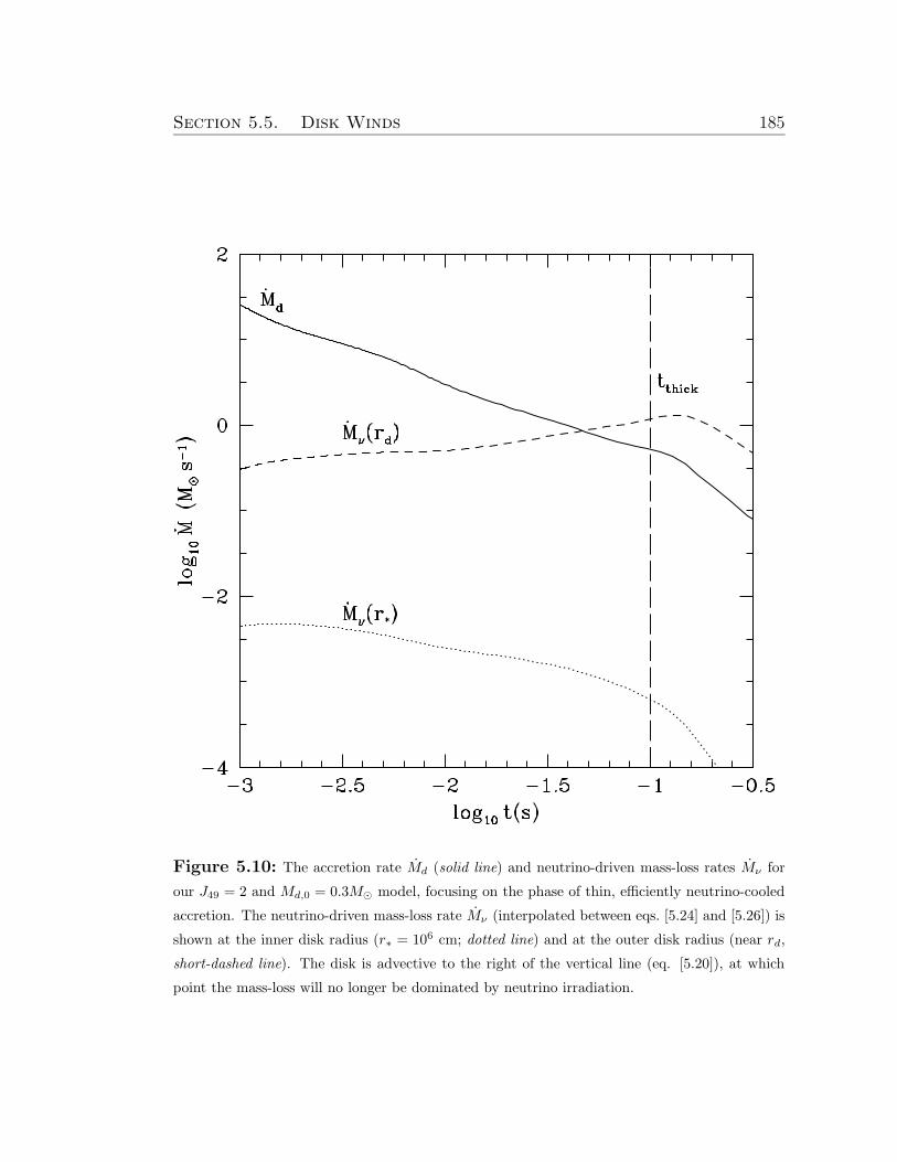
Section 5.5. Disk Winds 185
Figure 5.10: The accretion rate Md (solid line) and neutrino-driven mass-loss rates Mν for
our J49 = 2 and Md,0 = 0.3M¯ model, focusing on the phase of thin, efficiently neutrino-cooled
accretion. The neutrino-driven mass-loss rate Mν (interpolated between eqs. [5.24] and [5.26]) is
shown at the inner disk radius (r∗ = 106 cm; dotted line) and at the outer disk radius (near rd,
short-dashed line). The disk is advective to the right of the vertical line (eq. [5.20]), at which
point the mass-loss will no longer be dominated by neutrino irradiation.
Section 5.5. Disk Winds 186
parameter, a powerful viscously-driven outflow is likely (Blandford & Begelman
1999; Stone & Pringle 2001; Proga & Begelman 2003).
In §5.4.1 we showed that the disk becomes radiatively inefficient external to
an “ignition radius” rign ∝ M6/5d (eq. [5.19]). The outer disk, near rd, thickens first
(when rd ∼ rign at t ∼ tthick) and radiatively inefficient conditions move inwards as
Md decreases. In the simplest picture, one might expect that the innermost radii
become an RIAF only once Md drops from its value at t ∼ tthick by an additional
factor ∼ (r∗/rd)5/6. In fact, the entire disk probably become radiatively ineffi-
cient on a timescale similar to tthick if the accretion rate which reaches small radii
abruptly decreases once the outer disk thickens (Fig. 5.6). Hence, at a time tthick, a
significant portion of the accreting matter may be redirected into an outflow, with
only a fraction ∼ (r∗/rd) reaching small radii and accreting onto the BH (Stone &
Pringle 2001).
X-ray binaries typically produce radio jets upon transitioning from their “high-
soft” (radiatively efficient) to “low-hard” (radiatively inefficient) states (e.g., Remil-
lard & McClintock 2006). In analogy, once the inner disk becomes an RIAF,
conditions seem to favor the production of relativistic jets (see also Lazzati et
al. 2008).9
Even if only a fraction (r∗/rd) of the mass remaining when the disk thickens
actually reaches the origin, the total energy supply available would be
Ejet ≡ εjetMd(tthick)c2
(
r∗rd(tthick)
)
' 3× 1050(εjet0.1
)( r∗106cm
)
α6/170.1 M
−4/173
(
J492
)8/17
ergs,
(5.29)
where εjet is the fraction of the accretion energy used to power a jet and we
have estimated Md(tthick) and rd(tthick) using the self-similar thick disk solutions
(eqs. [5.46] and [5.48], respectively). Equation (5.29) shows that the accretion en-
ergy available from near r∗ following the RIAF transition is more than sufficient9This is in stark contrast to jets powered by neutrino annihilation along the polar axis, which
require a high radiative efficiency.
Section 5.5. Disk Winds 187
to power the late-time X-ray flares observed following some short GRBs. If this is
the case, tthick sets a characteristic timescale for late-time central engine activity.
If α . 10−3, tthick may be large enough to explain the ∼ 30 s delay until flaring
observed for some short GRBs (e.g., Berger et al. 2005; Villasenor et al. 2005).
However, very late time energy injection, such as the Chandra flare observed two
weeks after GRB050709 (Fox et al. 2005), appears to require an alternative ex-
planation. In addition, given observational evidence for α ∼ 0.1 in a number of
environments (King et al. 2007), it may be more natural to associate Ejet and tthick
with the energy and duration, respectively, of the short GRB itself, rather than
the late-time central engine activity (see §5.6).
5.5.3 Outflow Nuclear Composition
The outflow nuclear composition has important consequences for the observ-
able signature of compact object mergers. Nonrelativistic outflows are sufficiently
dense to synthesize heavy isotopes (Pruet et al. 2004; Surman et al. 2006), which
may power transient emission via radioactive decay. The isotopic yield depends
on the speed, thermodynamic properties, and the asymptotic electron fraction Y ae
in the outflow.10 Although relativistic winds from the inner disk are unlikely to
synthesize anything heavier than He (Lemoine 2002; Beloborodov 2003a), Y ae is
important in this case as well. A neutron-rich outflow may alter the jet’s dynamics
and the prompt and afterglow emission from that of the standard GRB fireball
model (e.g., Derishev et al. 1999; Beloborodov 2003b; Rossi et al. 2006).
Figure 5.11 delineates different regimes of outflow properties and composition
(as given by Y ae ) as a function of the wind launching radius r and accretion rate
Md. We fix α = 0.1 and M = 3M¯. The time-dependent evolution of the ring
radius rd is shown for a solution with J49 = 2 and Md,0 = 0.3M¯ (solid line).
At each time a given steady-state disk profile can be read off of this plot as a
horizontal line that extends from the far left and ends on rd. Therefore, outflows
10The asymptotic electron fraction is germane because heavy nuclei primarily form after freeze-out from β-equilibrium.
Section 5.5. Disk Winds 188
from radii interior to rd contribute to the disk’s total nucleosynthetic yield.
The ignition radius rign (eq. [5.19]) is shown in Figure 5.11 with a short dashed
line. For r & rign the disk is an RIAF and marked in the figure as “Thick Disk.”
In this case, a viscously driven outflow dominates (§5.5.2). Since outflows from
RIAFs escape the disk in roughly the accretion timescale, these winds retain the
midplane electron fraction (Chapter 4), so that Y ae ' Y mid
e ¿ 0.5 (because the
disk itself freezes-out neutron-rich, as summarized in §5.4.2 and Fig. 5.9).
For r . rign, the disk is efficiently neutrino-cooled and marked in Figure 5.11 as
“Thin Disk.” The absorption of neutrinos, which heats the outflow and unbinds it
from the BH may also alter its nucleonic composition. This drives Y ae to a value set
by the neutrino radiation field Y νe , which in general is different from Y mid
e . A simple
criterion was discussed in Chapter 4 for determining when Y ae ' Y ν
e . A typical
nucleon in the accretion disk at radius r must absorb an energy ' GMmN/2r to
become unbound from the BH, so that Nν ' GMmN/2r〈εν〉 neutrinos must be
absorbed per nucleon. If we take Nν > Q ∼ 2 − 3, then a typical nucleon has
changed its identity (p→ n or n→ p) at least several times.
This implies that all purely neutrino-driven outflows from radii smaller than
rν ≡GMmp
2Q〈εν〉' 107M3〈ε10〉
−1(Q/2)−1 cm, (5.30)
where 〈εν〉 ≡ 10〈ε10〉 MeV, achieve Y ae ' Y ν
e , independent of the disk’s midplane
composition.
We plot rν with Q = 2 as a dotted line in Figure 5.11, where 〈εν〉 is calcu-
lated from Md using our steady-state disk solutions (see §5.5.1). For r . rν , any
neutrino-driven outflow enters equilibrium with the neutrino radiation field (i.e.,
Y ae ' Y ν
e ). For r & rν the outflow approximately retains the midplane electron
fraction (i.e., Y ae ' Y mid
e ).
Although we have established the conditions under which Y ae is determined
by neutrino absorptions, we must now address what sets Y νe itself. If the rate of
neutrino absorptions exceeds the rate of degenerate pair captures before the wind
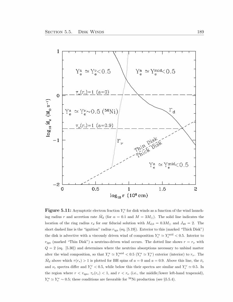
Section 5.5. Disk Winds 189
Figure 5.11: Asymptotic electron fraction Y ae for disk winds as a function of the wind launch-
ing radius r and accretion rate Md (for α = 0.1 and M = 3M¯). The solid line indicates the
location of the ring radius rd for our fiducial solution with Md,0 = 0.3M¯ and J49 = 2. The
short dashed line is the “ignition” radius rign (eq. [5.19]). Exterior to this (marked “Thick Disk”)
the disk is advective with a viscously driven wind of composition Y ae ' Y mid
e < 0.5. Interior to
rign (marked “Thin Disk”) a neutrino-driven wind occurs. The dotted line shows r = rν with
Q = 2 (eq. [5.30]) and determines where the neutrino absorptions necessary to unbind matter
alter the wind composition, so that Y ae ' Y mid
e < 0.5 (Y ae ' Y ν
e ) exterior (interior) to rν . The
Md above which τ(r∗) > 1 is plotted for BH spins of a = 0 and a = 0.9. Above this line, the νe
and νe spectra differ and Y νe < 0.5, while below this their spectra are similar and Y ν
e ' 0.5. In
the region where r < rign, τν(r∗) < 1, and r < rν (i.e., the middle/lower left-hand trapezoid),
Y ae ' Y ν
e ∼ 0.5; these conditions are favorable for 56Ni production (see §5.5.4).
Section 5.5. Disk Winds 190
falls out of β-equilibrium, Y νe is
Y νe ≡
(
1 +LνeLνe
〈ενe〉 − 2∆ + 1.2∆2/〈ενe〉
〈ενe〉+ 2∆ + 1.2∆2/〈ενe〉
)−1
, (5.31)
where ∆ = 1.293 MeV is the neutron-proton mass difference, and Lνe/Lνe and
〈ενe〉/〈ενe〉 are the mean νe/νe luminosities and energies, respectively, from a centrally-
concentrated source (Qian et al. 1993; QW96). Equation (5.31) demonstrates that
the νe and νe spectra are crucial for setting Y νe .
Since the disk’s luminosity and temperature peak at just a few rg, Yνe is
primarily determined by conditions at small radii. At early times, the accretion
disk may be optically thick near r∗ and so the νe and νe spectra depend on the
temperatures at νe and νe neutrinospheres, respectively. Since there are more
neutrons than protons in the disk, the optical depth to νe through the disk is
higher than to νe; thus, the temperature at the νe neutrinosphere is higher than at
the νe neutrinosphere. This implies Lνe À Lνe , 〈ενe〉 À 〈ενe〉, and thus Y νe ¿ 0.5.
Using 3-dimensional calculations of the merger of NSs with zero spin, Rosswog &
Liebendorfer (2003) find that at ∼ 15 ms following merger, Lνe ' 3.5Lνe , 〈ενe〉 ' 9
MeV, and 〈ενe〉 ' 15 MeV, which implies Y νe ' 0.21, consistent with our arguments
(see also Surman et al. 2008). We conclude that when the disk is optically-thick
near r∗, a neutron-rich outflow is again the most likely outcome. The critical
accretion rate at which τν(r∗) = 1 is shown in Figure 5.11 with a long dashed line
for both a = 0 and a = 0.9.
Once the disk becomes optically thin near r∗, the difference between the νe
and νe spectra is much less pronounced. This occurs because (1) the neutrinos
and antineutrinos originate from regions with the same temperature; (2) any net
lepton flux out of the disk must remain modest (i.e., Lνe/〈ενe〉 ' Lνe/〈ενe〉); and
(3) the difference between the e− and e+ capture cross sections for kT À ∆−mec2
is small. Taking 〈ενe〉 ∼ 〈ενe〉 À ∆, equation (5.31) shows that Y νe ' 0.5, a
value in the range required to produce 56Ni (which we discuss further in §5.5.4).
Indeed, Chapter 4 used the steady-state, optically-thin α-disk calculations of Chen
& Beloborodov (2007; hereafter CB07) to calculate the neutrino radiation fields
carefully, and showed that Y νe & 0.5 over the majority of the disk (see their Fig. 1).
Section 5.5. Disk Winds 191
Although the precise spectra extracted from an α-disk calculation should be taken
with caution, the conclusion that the νe and νe spectra are similar for optically
thin accretion (and Y νe ' 0.5) is probably robust.
Figure 5.11 illustrates that under most conditions the outflows from hyper-
accreting disks are neutron-rich. Neutron-rich material ejected during the initial
dynamical phase of compact object mergers has long been considered a promising
source for producing Galactic r-process elements, whose precise astrophysical ori-
gin remains uncertain (Lattimer & Schramm 1974; see, however, Qian 2000). In
addition, Surman et al. (2008) find that winds driven from the remnant accretion
disk at early times (when it is optically thick; upper left quadrant of Fig. 5.11)
are sufficiently neutron-rich to produce successful r-process. The outflows driven
from the advective disk at late times, however, are unlikely to produce r-process
elements, given their modest entropies and electron fractions of Ye & 0.3 (Figs. 5.8
and 5.9). Instead, this modest Ye material will be synthesized to form intermediate
mass neutron rich isotopes (Hartmann et al. 1985).
5.5.4 56Ni Production and Optical Transients
As summarized in Figure 5.11, most of the material in the outflow driven from
a hyper-accreting disk will be neutron-rich. Nonrelativistic neutron-rich ejecta are
difficult to detect because isotopes synthesized from low Ye material are themselves
very neutron-rich and typically possess very short half-lives, on the order of seconds
(e.g., Freiburghaus et al. 1999). Thus, most of the radioactive energy is released
at high optical depths and suffers severe adiabatic losses before the photons can
diffusively escape. By contrast, ejecta with Y ae ' 0.5 are easier to detect because
they can produce a significant quantity of 56Ni (Hartmann et al. 1985), an isotope
better suited to powering observable emission because its half-life ' 6 days is com-
parable to the timescale on which the outflow becomes optically thin. From Figure
5.11 we see that outflows in a modest range of parameter space (middle/lower-left
trapezoid) are capable of synthesizing 56Ni. One caveat to this conclusion is that
it only applies if the winds are primarily neutrino driven. If the outflow is instead
Section 5.5. Disk Winds 192
magnetocentrifugally driven by a moderately strong open poloidal magnetic field
(e.g., Levinson 2006; Xie et al. 2007), then Y ae ¿ 0.5 can result, even if Y ν
e ' 0.5
(Chapter 4). In what follows we assume that the wind’s are primarily neutrino
driven.
Under this assumption, Figure 5.12 shows the total 56Ni mass,
MNi = (XNi/0.4)MYe=0.5, produced in outflows from hyper-accreting disks as a
function of the disk’s initial mass Md,0 and radius rd,0, where MYe=0.5 is the total
mass-loss with Y ae ' 0.5 and XNi is the average 56Ni mass fraction synthesized
in the wind. We calculate MYe=0.5 by integrating the neutrino-driven mass-loss
(eqs. [5.24] and [5.26]) across the Y ae ' 0.5 region in Figure 5.11, using rd(t) and
Md(t) from the disk evolution calculations described in §5.4.
Pruet et al. (2004) present calculations of XNi which are parameterized in
terms of the asymptotic entropy Sa, mass-loss rate Mw, and asymptotic velocity
va of an outflow with Y ae ' 0.51. The mass MYe=0.5 is dominated by outflows from
radii ∼ 3 × 10⁶ − 107 cm when Md ∼ 0.1 − 1M¯ s−1 (corresponding to L52 ∼
few); equation (5.25) thus gives Sa ∼ 10 − 30kB baryon−1 for the ejecta with
Y ae ' 0.5. Purely neutrino-driven winds achieve asymptotic velocities which are
typically below the escape speed of the central object (e.g., Thompson et al. 2001);
thus, the asymptotic kinetic energy is most likely dominated by energy released
during the formation of heavy elements. Because ∼ 8 MeV baryon−1 is released in
producing Fe-peak elements, we estimate that va ' 0.1 − 0.15 c. Applying these
wind parameters to Figure 3 of Pruet et al. (2004), we estimate thatXNi ∼ 0.2−0.5,
thereby justifying our scaling for XNi in Figure 5.12.
Figure 5.12 shows that for large initial disk masses (Md,0 & 0.1M¯), the
ejected Ni mass, ∼ 3× 10⁻⁴ − 10−3M¯, can be appreciable. Disks with moderate
initial radii rd,0 ∼ 107 cm are optimal for producing 56Ni because they are suffi-
ciently large to contain the radius rν ∼ 107 cm and yet are sufficiently compact
to have a large initial accretion rate, which maximizes the neutrino luminosity
and thus the neutrino-driven mass-loss. Conveniently, initial disk parameters from
many compact object merger simulations (see §5.2) are in the range required to
produce ∼ 10−4 − 10−3M¯ of Ni.
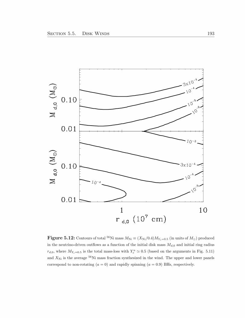
Section 5.5. Disk Winds 193
Figure 5.12: Contours of total 56Ni massMNi ≡ (XNi/0.4)MYe=0.5 (in units ofM¯) produced
in the neutrino-driven outflows as a function of the initial disk mass Md,0 and initial ring radius
rd,0, where MYe=0.5 is the total mass-loss with Y ae ' 0.5 (based on the arguments in Fig. 5.11)
and XNi is the average 56Ni mass fraction synthesized in the wind. The upper and lower panels
correspond to non-rotating (a = 0) and rapidly spinning (a = 0.9) BHs, respectively.
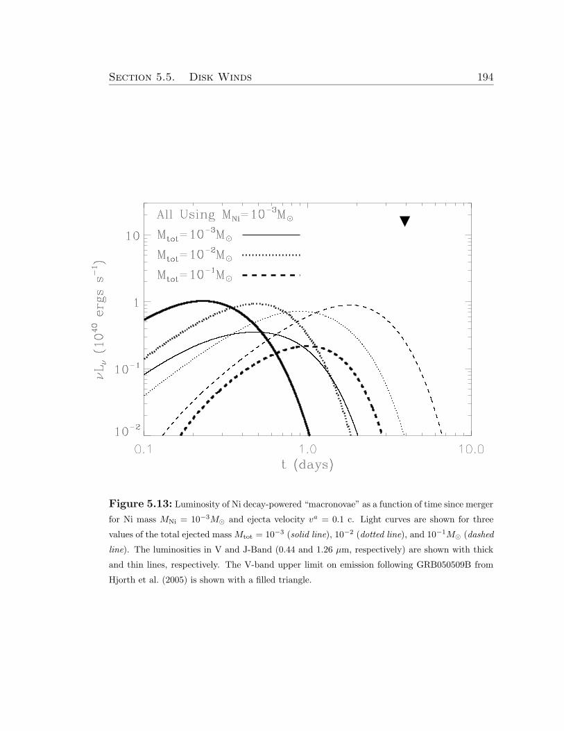
Section 5.5. Disk Winds 194
Figure 5.13: Luminosity of Ni decay-powered “macronovae” as a function of time since merger
for Ni mass MNi = 10−3M¯ and ejecta velocity va = 0.1 c. Light curves are shown for three
values of the total ejected massMtot = 10−3 (solid line), 10−2 (dotted line), and 10−1M¯ (dashed
line). The luminosities in V and J-Band (0.44 and 1.26 µm, respectively) are shown with thick
and thin lines, respectively. The V-band upper limit on emission following GRB050509B from
Hjorth et al. (2005) is shown with a filled triangle.
Section 5.5. Disk Winds 195
The decay of MNi ∼ 10−4 − 10−3M¯ can reheat the (adiabatically cooled)
ejecta sufficiently to produce detectable transient emission. In order to explore this
possibility, we calculate the light curves of ejecta heated by Ni decay (“macrono-
vae”) using the method of Kulkarni (2005). This simplified one-zone model ac-
counts for the fraction of the gamma-rays produced by the Ni decay which are
absorbed by the expanding material (Colgate et al. 1980) and assumes blackbody
emission at the photosphere, neglecting Comptonization.
Figure 7.3 shows the V and J-band luminosities as a function of time since
the merger for an outflow with Ni mass MNi = 10−3M¯ which is expanding at
va = 0.1 c. The V-band light curve peaks earlier because the temperature at the
photosphere decreases as the material expands. Somewhat after the peak in the
light curves, recombination will decrease the opacity well below that considered
here; thus our calculations are not quantitatively reliable at these times. The total
mass Mtot ejected during the merger event, most of it neutron rich, is likely to
be significantly larger than MNi; this provides additional opacity for the Ni-rich
material. To explore the effect of this additional material on the detectability of
the Ni decay, the light curves in Figure 7.3 are shown for three values of Mtot:
10−3M¯ (solid line), 10−2M¯ (dotted line), and 10−1M¯ (dashed line). As Figure
7.3 shows, larger Mtot: (1) delays the time to peak emission (tpeak is roughly
∝M1/2tot ); (2) increases the total fluence of the event by trapping a higher fraction
of the gamma-ray emission; and (3) increases the peak wavelength of the emission,
pushing it into the near-IR for large Mtot. We conclude that long wavelength
(λ & µm) observations at t ∼ 1 day are the most promising for the detection of a
Ni decay-powered macronova.
Hjorth et al. (2005) place an upper limit of mV > 27.5 at t = 3.9 days on any
emission associated with the short GRB 050509B (redshift z ' 0.22); we mark
this constraint in Figure 7.3 with an arrow. For Mtot = 0.1M¯ this constrains the
ejected Ni mass to be MNi . 10−2M¯ (see also Kulkarni 2005). As Figure 5.12
illustrates, compact object mergers are very unlikely to produce this much Ni, so
the absence of a detection thus far is unsurprising.
Section 5.6. Conclusion and Discussion 196
5.6 Conclusion and Discussion
We have calculated the time-dependent evolution of accretion disks formed
from compact mergers, and the properties of their outflows. Since most of the disk
mass resides at large radii, we approximate the disk as a ring at a given radius and
calculate the dynamics and composition of the ring as a function of time. This
ring model is calibrated to correctly reproduces the Green’s function solution for
a viscously spreading ring with viscosity ν ∝ r1/2 (appropriate for a thick disk;
see Appendix A). With this simplified model, we have studied the full parameter
space of remnant accretion disks (different initial masses, compositions, etc.) and
can follow the viscous evolution for arbitrarily long timescales.
The energetics of the ring at a given time can be described by one of three
models: (1) optically thick to neutrinos and advective, (2) optically thin to neu-
trinos and geometrically thin, and (3) optically thin to neutrinos and advective.
A massive, compact disk (with a short initial viscous time tvisc,0; eq. [5.5]) will
exhibit all three of these accretion phases, evolving from (1) to (3) as a function
of time (Figs. 5.1-5.4). Less massive disks, on the other hand, only pass through
phases (2) and (3), or even just (3). Note that these phases refer to the energetics
of the disk near the outer radius. At a given time, the disk may also undergo
similar transitions as a function of radius; e.g., a disk that is advective at large
radii will be neutrino cooled and geometrically thin inside the ignition radius rign
(eq. [5.19]).
Neutrino-driven winds during the early-time optically thick and neutrino-
cooled (thin disk) phases unbind so much mass that field lines connected to the
disk cannot produce sufficiently relativistic material to power short-duration GRBs
(§5.5.1 and Fig. 5.10). An alternative source for the relativistic material needed
to produce short GRBs are nearly baryon-free magnetic field lines that thread
the BH’s event horizon (e.g., McKinney 2005). In addition, when the inner disk
becomes advective (Md . 0.07α5/30.1 M¯ s
−1 for a = 0), conditions appear particu-
larly suitable for the formation of relativistic jets (by analogy to X-ray binaries,
which produce jets when making a similar transition; e.g., Remillard & McClintock
Section 5.6. Conclusion and Discussion 197
2006; see Lazatti et al. 2008 for a similar argument in the context of long-duration
GRBs).
Once the disk has transitioned to a late-time advective phase (phase 3 above),
the properties of the disk become well-described by self-similar solutions. Ignoring
for the moment outflows from the disk, these solutions are rd ∝ t2/3, Md ∝ t−1/3,
and Md ∝ t−4/3. Power-law variations in the disk properties are a generic feature of
a viscously evolving disk that conserves total angular momentum. These scalings
are not, however, likely to be applicable in practice because outflows during the
advective phase unbind most of the remaining material (§5.4.1 & 5.5.2). Energy
produced by fusion to He and heavier elements also contributes to driving an
outflow (Figs. 5.3 & 5.4). Such outflows remove a significant fraction of the
angular momentum of the disk. This leads to a much more rapid decrease in the
disk mass and accretion rate at late times (Appendix B3 and Fig. 5.6). Significant
accretion onto the central black hole will thus only last for a few viscous times
after the onset of the advective phase.
At the outer edge of the disk, the transition from a neutrino-cooled thin disk
to the late-time advective phase occurs at a time tthick ∼ 0.1α−23/170.1 (J49/2)
9/17
s (eq. [5.20]). The rapid decrease in Md after the onset of the advective phase
implies that the inner disk becomes advective at a similar time (§5.5.2 and Fig.
5.6). Quantitatively, we find that for powerful winds with p = 1 (see eq. [5.49]),
the inner disk becomes advective at t ∼ 0.2, 5, and 100 sec, for α = 0.1, 0.01, and
0.001, respectively (for our fiducial model with an initial mass of 0.1M¯ and an
initial radius of ' 3×107 cm). Thus, for α ∼ 10−3, the timescale for the inner disk
to become advective is comparable to the onset of observed flaring at ∼ 30 sec in
some short GRBs (e.g., Berger et al. 2005). Given the slow decline in disk mass
with time before tthick, there is ample accretion energy available in the disk at this
point to power the observed flaring. However, there is observational evidence for
α ∼ 0.1 in a number of astrophysical disks (King et al. 2007); we thus doubt that
tthick is large enough to coincide with the onset of observed flaring. Instead tthick is
likely to be ∼ 0.1− 1 sec, comparable to the duration of the short GRB itself. In
this case, the rapid decrease in the disk mass and accretion rate in the advective
Section 5.6. Conclusion and Discussion 198
phase imply that the remnant accretion disk alone does not contain sufficient mass
at ∼ 30 sec to power the observed late-time activity from short GRBs, nor is there
any physical reason to expect a sudden change in the disk or jet properties at this
time.
A more likely source of late-time flaring in compact object merger models is
a continued inflow of mass at late times, such as is produced by the infalling tidal
tail found in Lee & Ramirez-Ruiz’s (2007) NS-NS merger simulations (see also
Rosswog 2007). Similarly, the BH-NS merger simulations of Faber et al. (2006a,b)
show that ∼ 0.03M¯ of material is ejected into highly eccentric orbits during the
merger, which returns to the BH on a timescale & 1 s. However, final conclusions
regarding the quantity and ubiquity of late-time fall-back from NS-NS and BH-NS
mergers must await full-GR simulations which include BH spin and realistic EOSs.
The second major focus of this paper has been on the composition of the accre-
tion disk and its outflows as a function of time. For initial disk properties expected
in compact object mergers (§5.2), the disk typically comes into β-equilibrium given
the high temperatures and densities at small radii. As material spreads to larger
radii, however, the composition of the disk freezes out before it becomes advective
at late times; at freeze-out the disk is modestly neutron rich, with an electron
fraction Ye ≈ 0.3 (§5.4.2 and Fig. 5.9). This neutron rich material – ∼ 10−2M¯
for typical initial disk parameters – is blown away once the disk enters the ad-
vective phase at ∼ tthick. These outflows are particularly interesting given the
low solar system abundance of material produced in nuclear statistical equilibrium
at Ye ∼ 0.3 (Hartmann et al. 1985). In a separate paper, we will study this
nucleosynthesis and its implications in more detail.
Although outflows from compact object merger accretion disks are neutron
rich in most circumstances, neutrino-driven winds from radii ' 106 − 107 cm at
accretion rates Md ∼ 0.03 − 1M¯ s−1 have electron fractions Ye ' 0.5, precisely
that required to synthesize significant amounts of 56Ni (Fig. 5.11). We have
calculated the total Ni mass ejected by compact object merger disks as a function
of their initial mass and radius (§5.5.4 and Fig. 5.12). Disks with initial masses
& 0.1M¯ can produce up to ∼ 10−3M¯ of 56Ni. The radioactive decay of this Ni
Section 5.6. Conclusion and Discussion 199
as the outflow expands to large radii will produce an optical and infrared transient
peaking ∼ 0.5 − 2 days after the merger, with a peak flux of νLν ' 1040 ergs s−1
(Fig. 7.3). Because the Ni mass is likely to be a small fraction of the total mass
of the ejecta (most of which is neutron rich), this transient is best detected at
∼ 1µm. As Figure 7.3 shows, current observational limits on SN-like transients
coincident with short GRBs are about a factor of ∼ 10 above our predictions.
However, somewhat deeper limits from a moderately closer burst could start to
put interesting constraints on short GRB progenitors. It is also possible that
the decay of some neutron-rich isotopes could heat the outflow and contribute to
the late-time thermal emission (although most such isotopes have very short half-
lives). This possibility should be investigated in future calculations using a nuclear
reaction network.
Although we have focused on short GRBs throughout this paper, many of
our results can be applied more broadly. For example, long-duration GRBs show
late-time activity and flaring similar to that seen in short GRBs (e.g., Falcone
et al. 2007). For the reasons described above, this activity is probably produced
by a continued inflow of mass at late times (fallback from the stellar progenitor’s
envelope) rather than solely by the viscous evolution of the small-scale disk. As
a final application of our results, we note that the accretion-induced collapse of
a white dwarf to a neutron star (AIC) is expected to produce a compact disk
of ∼ 0.1 − 0.5M¯ outside the newly formed neutron star’s surface (Dessart et al.
2006). The calculations presented here describe the evolution of this remnant disk,
with the one caveat that the composition of the disk in the AIC context may be
strongly affected by neutrino irradiation from the newly-formed neutron star.
Acknowledgements
We thank Josh Bloom, Davide Lazzati, and Daniel Perley for useful conversations.
A. L. P. is supported by the Theoretical Astrophysics Center at UC Berkeley. B. D.
M. and E. Q. are supported in part by the David and Lucile Packard Foundation,
NASA Grant NNG06GI68G, and a NASA GSRP Fellowship to B.D.M.
Section 5.7. Appendix A: Calibration of the Ring Model 200
5.7 Appendix A: Calibration of the Ring Model
The surface density Σ of an axisymmetric disk in a Keplerian potential with
constant total angular momentum evolves according to a diffusion equation (e.g.,
Frank et al. 2002):∂Σ
∂t=
3
r
∂
∂r
[
r1/2∂
∂r
(
νΣr1/2)
]
, (5.32)
where ν is the kinematic viscosity. Assuming that ν depends only on radius as a
power law, viz: ν = ν0(r/R0)n, equation (6.10) is linear and, for an initial surface
density distribution Σ(r, t = 0) = (M0/2πR0)δ(r − R0) which is narrowly peaked
about the radius R0, the solution (for n < 2) is given by
Σ(r, t) =M0(1− n/2)
πR20x
(n+1/4)τexp
[
−(1 + x2−n)
τ
]
I1/|4−2n|
[
2x1−n/2
τ
]
,
where M0 is the initial disk mass, x ≡ r/R0, τ ≡ t[12ν0(1− n/2)2/R2
0], and Im is
a modified Bessel function of order m. For small argument y ¿ 1, Im(y) takes the
asymptotic form Im ' (y/2)m/Γ(m + 1), where Γ is the Gamma function; thus,
for late times or small radii such that τ À 2x1−n/2, equation (5.33) reduces to
Σ(r, t)|τÀ2x1−n/2 =M0
πR20
(1− n/2)
Γ[5−2n4−2n
]
1
τ(5−2n4−2n)xn
exp
[
−(1 + x2−n)
τ
]
(5.34)
Most of the mass in the disk is located near the radius where the local mass
Md ∝ Σr2 peaks; using equation (5.34), at late times this radius is found to be
rpeak = R0τ1/(2−n). Hence, equation (5.34) becomes valid near rpeak for τ À 1.
The constant A, which relates the total disk mass at late times from the exact
solution of equation (6.10) to the mass defined by πΣ(rpeak)r2peak, can be calculated
from equation (5.34) to be
A(τ À 1) ≡
∫∞
02πΣrdr
πΣ(rpeak)r2peak
∣
∣
∣
∣
∣
τÀ1
=2e
2− n(5.35)
Similarly, the constant B, which relates the total disk angular momentum at late
times from the exact solution to that estimated by πΣr2peak(GMrpeak)1/2, is given
by
B(τ À 1) ≡
∫∞
02πΣr3/2dr
πΣ(rpeak)r5/2peak
∣
∣
∣
∣
∣
τÀ1
=2e
2− nΓ
[
5− 2n
4− 2n
]
(5.36)
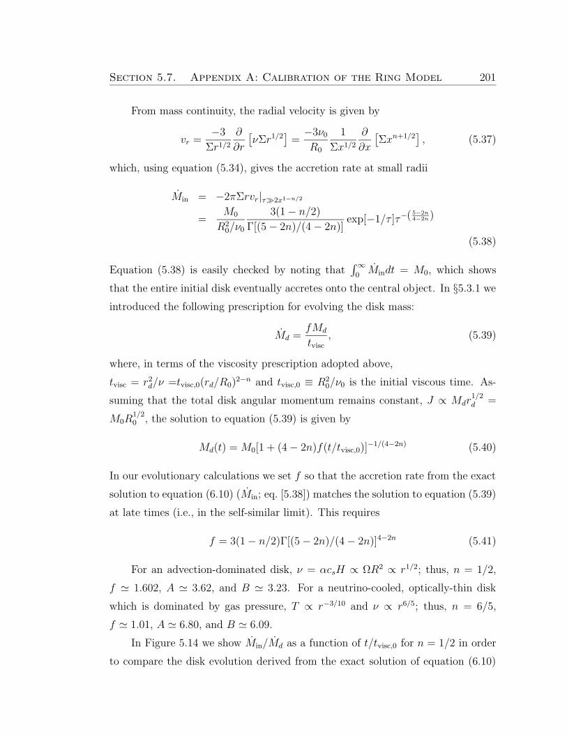
Section 5.7. Appendix A: Calibration of the Ring Model 201
From mass continuity, the radial velocity is given by
vr =−3
Σr1/2∂
∂r
[
νΣr1/2]
=−3ν0R0
1
Σx1/2∂
∂x
[
Σxn+1/2]
, (5.37)
which, using equation (5.34), gives the accretion rate at small radii
Min = −2πΣrvr|τÀ2x1−n/2
=M0
R20/ν0
3(1− n/2)
Γ[(5− 2n)/(4− 2n)]exp[−1/τ ]τ−(
5−2n4−2n)
(5.38)
Equation (5.38) is easily checked by noting that∫∞
0Mindt = M0, which shows
that the entire initial disk eventually accretes onto the central object. In §5.3.1 we
introduced the following prescription for evolving the disk mass:
Md =fMd
tvisc, (5.39)
where, in terms of the viscosity prescription adopted above,
tvisc = r2d/ν =tvisc,0(rd/R0)2−n and tvisc,0 ≡ R2
0/ν0 is the initial viscous time. As-
suming that the total disk angular momentum remains constant, J ∝ Mdr1/2d =
M0R1/20 , the solution to equation (5.39) is given by
Md(t) = M0[1 + (4− 2n)f(t/tvisc,0)]−1/(4−2n) (5.40)
In our evolutionary calculations we set f so that the accretion rate from the exact
solution to equation (6.10) (Min; eq. [5.38]) matches the solution to equation (5.39)
at late times (i.e., in the self-similar limit). This requires
f = 3(1− n/2)Γ[(5− 2n)/(4− 2n)]4−2n (5.41)
For an advection-dominated disk, ν = αcsH ∝ ΩR2 ∝ r1/2; thus, n = 1/2,
f ' 1.602, A ' 3.62, and B ' 3.23. For a neutrino-cooled, optically-thin disk
which is dominated by gas pressure, T ∝ r−3/10 and ν ∝ r6/5; thus, n = 6/5,
f ' 1.01, A ' 6.80, and B ' 6.09.
In Figure 5.14 we show Min/Md as a function of t/tvisc,0 for n = 1/2 in order
to compare the disk evolution derived from the exact solution of equation (6.10)
Section 5.8. Appendix B: Analytic Self-Similar Solutions 202
to that calculated from our simplified model. Figure 5.14 also shows the ratio
of the total disk mass Mtot ≡∫∞
02πΣrdr calculated from equation (5.33) to the
disk mass Md (eq. [5.40]) of the simplified model, as well as the ratio of rpeak (the
radius where Σr2 peaks, using eq. [5.33] for Σ) to the radius determined by angular
momentum conservation: rd = R0(Md/M0)2. Figure 5.14 shows that, although the
accretion rate in the two models differ at very early times (the initially narrowly-
concentrated ring takes a short period of time to spread to small radii), they
approach one another to . 20% by t & 0.1tvisc,0. Likewise, the disk mass and radii
from the exact solution and simplified model are quite similar at all times.
The numerical values for A and B given in equations (5.35) and (5.36) and
employed in our calculations apply only to the mass and angular momentum distri-
bution in the disk at late times (τ À 1). Initially, the disk is entirely concentrated
at a single radius and A(t = 0) = B(t = 0) = 1; thus, A(t) and B(t) evolve
significantly from early times until the disk enters the self-similar limit and so one
might worry that the early-time description of the disk’s evolution depends sensi-
tively on the initial mass distribution. Our model only assumes, however, that the
ratio A(t)/B(t) remains constant, which is a good approximation. To illustrate
this, Figure 5.14 shows A(t)/B(t) calculated from the exact solution (eq. [5.33])
for n = 1/2. Note that A(t)/B(t) increases from unity to its asymptotic value
A/B = Γ[(5− 2n)/(4− 2n)], which is ' 1.12 for n = 1/2.
5.8 Appendix B: Analytic Self-Similar Solutions
The late-time evolution of our disk calculations asymptote to power laws that
are well approximated by analytic self-similar solutions. We derive these here to aid
in interpreting our numerical results. Presentation is divided between neutrino-
cooled, thin-disk solutions and late-time advective solutions. One could just as
well derive analogous results for disks that are optically thick to neutrinos. We
forgo this here since the initial viscous time is always sufficiently long that these
solutions are never applicable to our numerical results. We conclude by presenting
self-similar solutions for advective disks with substantial mass-loss, since these
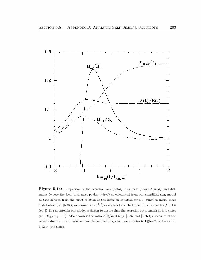
Section 5.8. Appendix B: Analytic Self-Similar Solutions 203
Figure 5.14: Comparison of the accretion rate (solid), disk mass (short dashed), and disk
radius (where the local disk mass peaks; dotted) as calculated from our simplified ring model
to that derived from the exact solution of the diffusion equation for a δ−function initial mass
distribution (eq. [5.33]); we assume ν ∝ r1/2, as applies for a thick disk. The parameter f ' 1.6
(eq. [5.41]) adopted in our model is chosen to ensure that the accretion rates match at late times
(i.e., Min/Md → 1). Also shown is the ratio A(t)/B(t) (eqs. [5.35] and [5.36]), a measure of the
relative distribution of mass and angular momentum, which asymptotes to Γ[(5−2n)/(4−2n)] '
1.12 at late times.
Section 5.8. Appendix B: Analytic Self-Similar Solutions 204
differ significantly from the solutions without mass-loss.
5.8.1 Neutrino-Cooled, Thin-Disk Solutions
In the neutrino-cooled, thin-disk limit, the cooling is dominated by Urca, and
the pressure is given by ideal gas. Combining local energy balance and continuity,
Md = fAπνΣ, allows us to solve for the temperature and column density as
functions of radius. We substitute these into the angular momentum equation,
B(GMrd)1/2πr2dΣ = Jd, to solve forMd as a function of Md and Jd. We then assume
the solutions have a self-similar form of Md ∝ t−β, so that Md = −dMd/dt =
βMd/t. In this way we solve for β = 5/8, Md(t), and subsequently any other
variable of interest. The results are
Md = 1.3× 10⁻²f−5/81.6
(
A3.6
B3.2
)
α−3/40.1 M
−1/43
(
J492
)
t−5/8M¯, (5.42)
Md = 2.7× 10⁻²f−5/81.6
(
A3.6
B3.2
)
α−3/40.1 M
−1/43
(
J492
)
t−13/8M¯s−1 (5.43)
and
rd = 4.1× 10⁸f5/41.6 α
3/20.1M
−1/23 t5/4cm. (5.44)
where f1.6 = f/1.6, A3.6 = A/3.6, B3.2 = B/3.2, and t is measured in seconds, and
the prefactors have been scaled to match our numerical results. The first thing to
notice is that both Md and Md are rather insensitive to the choice of f as long as
it is near unity, and A and B only appear as a ratio, which is also nearly unity.
This provides confidence in using this parameterization, and these specific values
for the corresponding parameters, when the disk is not well-described by n = 1/2.
This analysis also demonstrates the relative dependence on α. In Figure 5.15 we
compare these scaling (dotted lines) with the numerical calculations. This shows
that these solutions are only applicable for a short time. At times when t < tvisc
the evolution is much flatter and is dominated by initial conditions. At later times
the disk becomes advective and the solutions of the next section apply.
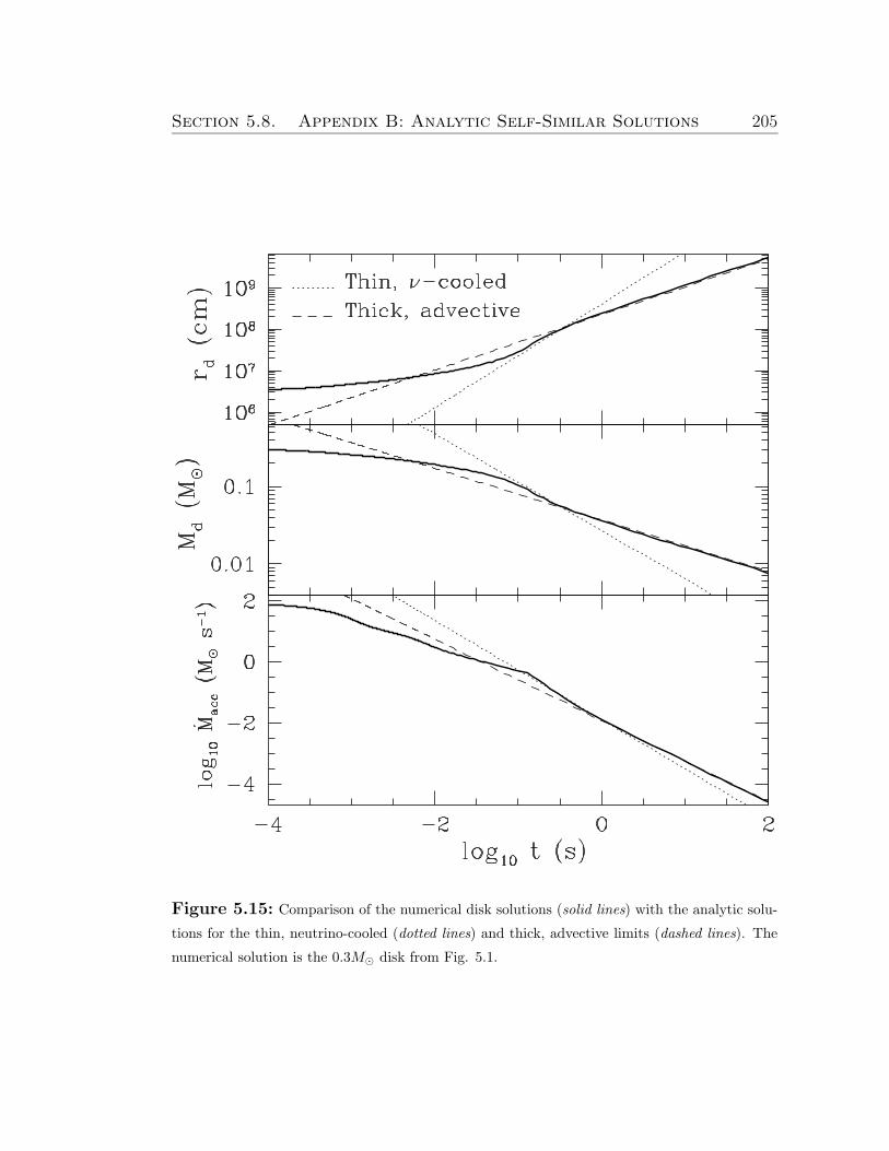
Section 5.8. Appendix B: Analytic Self-Similar Solutions 205
Figure 5.15: Comparison of the numerical disk solutions (solid lines) with the analytic solu-
tions for the thin, neutrino-cooled (dotted lines) and thick, advective limits (dashed lines). The
numerical solution is the 0.3M¯ disk from Fig. 5.1.
Section 5.8. Appendix B: Analytic Self-Similar Solutions 206
5.8.2 Late-Time Advective Solutions
In this limit, self-similar solutions can be found in an analogous way. The
viscous energy release is carried by advection with the internal energy dominated
by relativistic particles, so that
9
8fAπΩ2M = Vr
H
r
11
6aT 4. (5.45)
Combining this with mass continuity, gives the column depth as a function of ra-
dius, Σ(r) = (16/9Aπα)(M/r2Ω). We then use this relation withB(GMrd)1/2Md =
Jd and Md = βMd/t, to find β = 1/3 and the self-similar solutions
Md = 3.7× 10⁻²(
A3.6
B3.2
)
α−1/30.1 M
−2/33
(
J492
)
t−1/3M¯, (5.46)
Md = 1.2× 10⁻²(
A3.6
B3.2
)
α−1/30.1 M
−2/33
(
J492
)
t−4/3M¯s−1, (5.47)
and
rd = 2.3× 10⁸α2/30.1M
1/33 t2/3cm. (5.48)
These advective results are even more insensitive to A, B, and f than the thin-
disk results. Equation (5.46)-(5.48) are plotted in Figure 5.15 as dashed lines. The
numerical calculations follow these solutions very closely for times later than tthick
(given by eq. [5.20]).
Equations (5.46)-(5.48) can also be derived ignoring equation (5.45), but as-
suming that the scaleheight is fixed at H/r ' 0.6. This introduces the additional
dependencies Md ∝ (H/r)−2/3, Md ∝ (H/r)−2/3, and rd ∝ (H/r)4/3, but gives
nearly identical prefactors.
5.8.3 Advective Solutions with Mass-Loss
In §5.5.2 we described how advective disks are likely to lose a substantial
fraction of their mass to viscously driven outflows. Because the outflow removes
angular momentum as well – at least the specific angular momentum of the mass
that is lost – the disk need not expand as rapidly to large radii. In addition, the
disk mass and accretion rate decrease much more rapidly at late times than in the
Section 5.8. Appendix B: Analytic Self-Similar Solutions 207
self-similar solutions described in the previous subsection. To quantify this effect,
we follow Blandford & Begelman (1999) and assume that only a fraction ∼ (r∗/rd)p
of the available material is accreted onto the central BH. The remainder is lost to
an outflow. Thus the outflow rate at any time is given by
Mout =
(
1−
[
r∗rd
]p)fMd
tvisc(5.49)
We further assume that the angular momentum-loss rate from the disk is given by
J = −CMout (GMrd)1/2 . (5.50)
where C is a constant that depends on the torque exerted by the outflowing mass
on the remaining disk. If the outflow produces no net torque, an assumption that
appears at least qualitatively consistent with the relatively small-scale magnetic
fields seen in global MHD disk simulations (e.g., Stone & Pringle 2001), then the
angular momentum-loss is only that due to the specific angular momentum of the
outflow, and (Kumar, Narayan, & Johnson 2008)
C =2p
2p+ 1. (5.51)
We solve equations (5.6), (5.7), (5.49), and (5.50), assuming A/B = 1 and ν ∝ r1/2
(as appropriate for a thick disk). The solution depends on the relative magnitude
of 1− C and C(r∗/rd)p. For C(r∗/rd)
p ¿ 1− C, which is true at nearly all times
if equation (5.51) is applicable, then
rd ' rd,0
[
1 + 3f(1− C)
(
t
tvisc,0
)]2/3
, (5.52)
Md 'Md,0
[
1 + 3f(1− C)
(
t
tvisc,0
)]−1/[3(1−C)]
, (5.53)
and
Min ' fMd,0
tvisc,0
(
r∗rd,0
)p
×
[
1 + 3f(1− C)
(
t
tvisc,0
)]−[1+3(1+2p/3)(1−C)]/[3(1−C)]
(5.54)
Section 5.8. Appendix B: Analytic Self-Similar Solutions 208
Note that if p = C = 0 (i.e., no mass or angular momentum-loss), then these self-
similar solutions reduce to those of the previous subsection. However, for the case
p = 1 consistent with a number of global advective disk simulations (e.g., Hawley
& Balbus 2002), and in the absence of a net torque on the disk, C = 2/3 and
these solutions correspond to rd ∝ t2/3, Md ∝ t−1, and Min ∝ t−8/3 (see also Fig.
5.6). This shows that the disk mass and accretion rate decrease subsantially more
rapidly in time than in the absence of an outflow, while the disk expands outward
at roughly the same rate. If there is a net torque on the disk such that C ' 1,
then equations (5.52)–(5.54) are not applicable. Instead, for C(r∗/rd)p À 1 − C,
the solution is given by (for p 6= 0 and tÀ tvisc,0)
rd(t) '[
(3 + 2p)frp∗r1.5d,0
]1/(1.5+p)(
t
tvisc,0
)1/(1.5+p)
(5.55)
and
Md(t) 'Md,0 exp[−D(t/tvisc,0)p/(1.5+p)] (5.56)
where
D =
(
1.5 + p
p (3 + 2p)1.5/(1.5+p)
)
(
fr1.5d,0[frp∗r1.5d,0]
1.5/(1.5+p)
)
. (5.57)
For p = 1 and for rd,0 ∼ r∗, these solutions become rd(t) ∼ rd,0(t/tvisc,0)2/5 and
Md(t) ∼ Md,0 exp[−1.15(t/tvisc,0)2/5]. The radius of the disk thus increases signif-
icantly more slowly, and the mass of the disk decreases much more rapidly, than
in the self-similar solutions without mass-loss.
The numerical solutions including mass-loss during the advective phase shown
in Figure 5.6 assume that equation (5.51) is applicable and are indeed well-described
by the self-similar solutions given in equations (5.52)-(5.54) at late times.
209
Chapter 6
Neutron-Rich Freeze-Out in
Accretion Disks Formed From
Compact Object Mergers
B. D. Metzger, A. L. Piro, E. Quataert (2009), MNRAS in press.1
Abstract
Accretion disks with masses ∼ 10−3 − 0.1M¯ are believed to form during the
merger of a neutron star (NS) with another NS and the merger of a NS with a
black hole (BH). Soon after their formation, such hyper-accreting disks cool effi-
ciently by neutrino emission and their composition is driven neutron-rich by pair
captures under degenerate conditions. However, as the disk viscously-spreads and
its temperature drops, neutrino cooling is no longer able to offset viscous heating
and the disk becomes advective. Analytic arguments and numerical simulations
suggest that once this occurs, powerful winds likely drive away most of the disk’s
remaining mass. We calculate the thermal evolution and nuclear composition
of viscously-spreading accretion disks formed from compact object mergers using
one-dimensional height-integrated simulations. We show that freeze-out from weak
1Copyright 2009. Royal Astronomical Society. All rights reserved.
Section 6.1. Introduction 210
equilibrium necessarily accompanies the disk’s late-time transition to an advective
state. As a result, hyper-accreting disks generically freeze out neutron-rich (with
electron fraction Ye ∼ 0.2 − 0.4), and their late-time outflows robustly synthesize
rare neutron-rich isotopes. Using the measured abundances of these isotopes in
our solar system, we constrain the compact object merger rate in the Milky Way
to be . 10−5(Md,0/0.1M¯)−1 yr−1, where Md,0 is the average initial mass of the
accretion disk. Thus, either the NS-NS merger rate is at the low end of current
estimates or the average disk mass produced during a typical merger is ¿ 0.1M¯.
Based on the results of current general relativistic merger simulations, the latter
constraint suggests that prompt collapse to a BH is a more common outcome of
NS-NS mergers than the formation of a transient hyper-massive NS. We also show
that if most short duration gamma-ray bursts (GRBs) are produced by compact
object mergers, their beaming fraction must exceed fb ≈ 0.13(Md,0/0.1M¯), cor-
responding to a jet half-opening angle & 30(Md,0/0.1M¯)1/2. This is consistent
with other evidence that short duration GRB outflows are less collimated than
those produced in long-duration GRBs.
6.1 Introduction
Massive, compact accretion disks are thought to form in a number of astro-
physical events, including the merger of a black hole and a neutron star (BH-NS;
Lattimer & Schramm 1974, 1976), the merger of a double NS binary (NS-NS;
Eichler et al. 1989), the collapse of a rapidly-rotating stellar core (Woosley 1993),
the accretion-induced collapse (AIC) of a white dwarf (WD) to a NS (Dessart
et al. 2006, 2007), and the AIC of a NS to a BH (Vietri & Stella 1998, 1999).
These disks are termed “hyper-accreting” due to their large accretion rates of up
to several solar masses per second. Rapid accretion onto a BH following the col-
lapse of a massive star is a popular model for the central engine of long-duration
gamma-ray bursts (GRBs) (MacFadyen & Woosley 1999) due to their associa-
tion with star forming regions and Type Ibc supernovae (SNe) (Woosley & Bloom
2006). Short-duration GRBs, on the other hand, originate from a more evolved
Section 6.1. Introduction 211
progenitor population (e.g., Berger et al. 2005) and may instead result from com-
pact object (CO) mergers (e.g., Lee & Ramirez-Ruiz 2007), or the AIC of a WD
(Chapter 3) or a NS (MacFadyen et al. 2005).
Hyper-accreting disks cool via neutrino emission when the accretion rate is
sufficiently high (M & 0.01−0.1M¯ s−1; Popham et al. 1999). This allows the disk
midplane to become dense and electron degenerate (Chen & Beloborodov 2007).
Because positron captures (e+ + n → p + νe) are suppressed relative to electron
captures (e− + p → n + νe) under degenerate conditions, neutrino-cooled disks
are driven neutron-rich (Pruet et al. 2003; Beloborodov 2003), i.e., to an electron
fraction Ye ≡ np/(np + nn) < 0.5, where np and nn are the proton and neutron
density, respectively.
If a portion of this neutron-rich material escapes the disk, several observable
consequences may result (e.g., Derishev et al. 1999). In particular, although highly
relativistic outflows are required to produce GRBs, slower outflows from larger
radii in the disk are probably at least as common (e.g., Pruet et al. 2004). These
dense outflows may synthesize heavy, neutron-rich isotopes as they expand away
from the midplane and cool. Such outflows are difficult to detect directly because
neutron-rich isotopes have short half-lives (∼ seconds; Freiburghaus et al. 1999)
and are thus unlikely to power a bright SN-like transient via their radioactive decay
(although a dimmer, shorter-lived transient may be produced; Li & Paczynski 1998;
Kulkarni 2005; Chapter 5).
Neutron-rich outflows can also be probed indirectly via their effect on the
chemical evolution of the Galaxy. For instance, moderately neutron-rich outflows
with Ye ≈ 0.35−0.4 produce isotopes (e.g., 79Br and 78Se) that are rare in our solar
system (Hartmann et al. 1985; Woosley & Hoffman 1992). Hence, the measured
abundances of these isotopes place stringent constraints on the rate at which low-
Ye material is ejected into the interstellar medium (ISM). In turn, if the amount
of neutron-rich material ejected in a given event can be estimated, the true rate
and beaming fraction (or jet opening angle) could in principle be constrained in
models that associate these events with GRBs (e.g., Woosley & Baron 1992; Fryer
et al. 1999). Constraints on the rate of CO mergers are particularly interesting
Section 6.1. Introduction 212
because they are the primary target for km-scale gravitational wave detectors such
as LIGO and VIRGO, and rates derived from known merging systems (Kalogera
et al. 2004; Kim et al. 2006) and population synthesis models (e.g., Belczynski et
al. 2006) remain highly uncertain.
6.1.1 Summary of Previous Work
Most previous efforts to determine the composition of outflows from hyper-
accreting disks have focused on winds driven by neutrino irradiation from the inner
disk (Levinson 2006; Surman et al. 2006, 2008; Barzilay & Levinson 2007; Chapter
4), in analogy to those from proto-neutron stars following successful core-collapse
SNe (e.g., Burrows, Hayes, & Fryxell 1995). However, the electron fraction at the
base of neutrino-driven outflows is typically not preserved as matter accelerates to
large radii because neutrino absorptions (p + νe → n + e+ and n + νe → p + e−)
drive Ye to the equilibrium value
Y νe ≈ [1 + (Lνe〈ενe〉/Lνe〈ενe〉)]
−1 (6.1)
given by the properties of the neutrino radiation field, where Lνe/Lνe and 〈ενe〉/〈ενe〉
are the mean νe/νe luminosities and energies, respectively, from the central NS or
accretion disk (Qian et al. 1993). When the accretion rate is very high (M &
M¯ s−1) and the inner disk is optically thick to neutrinos, Y νe can itself be ¿
0.5 because the νe’s originate from regions of higher temperature than the νe’s
(e.g., Surman et al. 2006). However, a disk with a fixed initial mass (such as is
produced by a CO merger) spends very little time (if any) accreting at such a
high rate; most neutrino-driven mass-loss from a viscously-spreading disk occurs
at later times, when the entire disk is optically thin and Y νe ∼ 0.5 (see Fig. 5.10).
Thus, while early-time neutrino-driven outflows may produce modest amounts
of r-process ejecta, their total yield in the context of CO mergers is probably
insufficient to contribute appreciably to the Galactic abundance of neutron-rich
isotopes (e.g., Surman et al. 2008). However, as we now discuss, later stages in the
disk’s evolution, when neutrino irradiation is relatively unimportant, are likely to
eject even larger quantities of neutron-rich material.
Section 6.1. Introduction 213
In a recent paper (Chapter 5), we used a one-zone (or “ring”) model to study
the evolution of hyper-accreting disks. Guided by analytic work (Blandford &
Begelman 1999) and numerical simulations (e.g., Stone & Pringle 2001; Haw-
ley, Balbus, & Stone 2001; Hawley & Balbus 2002) which show that radiatively-
inefficient accretion drives powerful outflows, we argued that the majority of the
disk becomes unbound soon following the disk’s transition to an advective state at
late times. Since ejection occurs on approximately the dynamical timescale (which
is faster than weak interactions at this stage), these “viscously-driven” outflows
maintain the electron fraction of the disk midplane, unlike the neutrino-driven
outflows at earlier times. Thus, in order to determine what isotopes are ultimately
synthesized, the electron fraction in the disk must be known at late times when
the disk becomes advective.
6.1.2 Outline of this Chapter
In this paper we determine the composition of late-time outflows from hyper-
accreting disks by calculating the disk’s midplane composition as the disk viscously-
spreads and falls out of weak equilibrium. We concentrate in particular on BH
accretion following a CO merger2 (either NS-NS or NS-BH models), where a fixed
initial disk mass is a reasonable approximation. In §6.2 we use a one-zone model
similar to that in Chapter 5 to calculate Ye(t) for a wide variety of plausible initial
disk masses and sizes. Although the one-zone model in §6.2 captures the basic
evolution of hyper-accreting disks, the subsequent nucleosynthesis depends sensi-
tively on the freeze-out electron fraction Y fe , and so a more detailed calculation is
warranted. Furthermore, a one-zone model cannot, by construction, address the
possibility that different annuli in the disk may freeze out with different values of
Y fe . Therefore in §6.3 we present one-dimensional (1D), height-integrated calcula-
tions of the evolution of CO merger disks and their composition, and use them to
determine the electron fraction mass distribution M(Y fe ) at late times. We find
2Although we center our discussion on accretion following CO mergers, most of our conclusionswould apply equally to the AIC of a NS to a BH, which may produce a disk with similar initialproperties (Shibata 2003; Shapiro 2004).
Section 6.2. One Zone Model 214
that under most conditions the majority of the mass freezes out neutron-rich with
Y fe ∼ 0.2 − 0.4. In §6.4 we summarize our results and use them to constrain the
CO merger rate and the beaming fraction of short GRBs.
6.2 One Zone Model
In this section we present calculations of the electron fraction at freeze-out
Y fe using a one-zone “ring” model similar to that presented in Chapter 5. The
simplicity of this model allows us to efficiently explore a wide parameter space
of initial disk mass Md,0 and radius rd,0, and it also provides a useful point of
comparison for our 1D calculations in §6.3. The initial conditions and relevant
equations are presented in §6.2.1. In §6.2.2 we present our results and show,
using a simple analytic argument, that a moderately neutron-rich freeze-out (i.e.,
Y fe . 0.5) is generically expected, relatively independent of the details of how the
disk viscously spreads.
6.2.1 Equations and Initial Conditions
Since the accretion disks produced during CO mergers are created from tidally
disrupted NS material, we take the initial electron fraction to be Y 0e = 0.1, which
is characteristic of the inner neutron star crust (e.g., Haensel & Zdunik 1990a,b;
Pethick & Ravenhall 1995). In most of our calculations we take the BH mass
to be MBH = 3M¯. The mass and radial profile of the remnant disks formed
from CO mergers are uncertain theoretically because they depend on the unknown
supranuclear-density equation of state and general relativistic effects, which are
now being explored in merger simulations (e.g., Shibata & Taniguchi 2006). Disk
masses Md ∼ 10−3 − 0.3M¯ with characteristic sizes ∼ 106 − 3 × 107 cm appear
typical (e.g., Rasio et al. 2005; Oechslin & Janka 2006; Shibata & Taniguchi 2006).
The equations and assumptions employed in our one-zone model closely fol-
low those in Chapter 5. To provide a brief summary, our calculation follows the
thermal and viscous evolution of the disk radius rd(t) (the “ring”) that contains
Section 6.2. One Zone Model 215
the majority of the mass, controls the accretion rate M onto the central object,
and moves outwards as the disk accretes in order to conserve the total angular
momentum J ∝ Mdr1/2d . Our energy equation includes viscous heating and the
dominant neutrino opacities. The model is calibrated so as to reproduce the ex-
act δ-function solution to the viscous diffusion equation (eq. [6.10]) at late times.
Although we refer the reader to Chapter 5 for details, we include here a brief dis-
cussion of changes and additions we have made and highlight the equations most
important for this work.
The electron fraction is evolved using
dYedt
= (λe+n+λνen)
[
1− Ye −
(
1−Xf
2
)]
−(λe−p+λνep)
[
Ye −
(
1−Xf
2
)]
, (6.2)
where d/dt is a Lagrangian derivative, λe−p/λe+n are the pair capture rates (see
Beloborodov 2003, eqs. [6], [7]), Xf is the free nucleon mass fraction in nuclear
statistical equilibrium (NSE) (from, e.g., Woosley & Baron 1992), and
λνN =LνσνNXN
4πr2d〈εν〉(1 + τνN)≈ 500
XNL52〈ε10〉
r26(1 + τνN)s−1 (6.3)
are the neutrino capture rates (e.g., Qian & Woosley 1996) due to irradiation
from the inner accretion disk (see the discussion below). In equation (6.3), νN
stands for either νen or νep, XN is the corresponding proton or neutron mass
fraction, Lν ≡ L521052 ergs s−1 is the neutrino luminosity, 〈εν〉 ≡ 10〈ε10〉 MeV is
the mean neutrino energy, and σνN ' 9 × 10−44〈ε2ν〉 MeV−2cm2 is the neutrino
capture cross section. The factor (1 + τνN) accounts for the possibility that the
absorbing annulus may become optically thick, where τνN ≡ σνNXNρrd/2mp is the
neutrino optical depth and ρ is the density; our calculation is fairly insensitive to
this prescription for when τν > 1, however, because τν is generally ¿ 1 at freeze-
out. We neglect the proton-neutron mass difference ∆ ≈ 1.3 MeV and the effects
of electron degeneracy in calculating σνN because the energies of the neutrinos
that dominate the heating (〈εν〉 ∼ 10 MeV) greatly exceed ∆ and the electron
Fermi energy, respectively. We assume relativistic e−/e+ pairs when calculating
the electron chemical potential; we have verified that this is a good approximation
by checking that including the effects of arbitrary e−/e+ energies has no significant
Section 6.2. One Zone Model 216
effect on the value of Y fe . NSE is a generally a good assumption in calculating Xf
because the entropy in the disk is sufficiently low that α−particles form while the
midplane temperature is still high (T & 0.5 MeV).
The dominant process that sets Ye during the thin disk phase is pair capture
on free nuclei (e.g., Pruet et al. 2003). However, neutrino absorptions become
important near freeze-out and must be included in a detailed calculation (see
Fig. 6.2). The neutrino absorption rate λνN is dominated by the high energy
neutrinos that are radiated from the smallest radii in the disk. We calculate
Lν and 〈εν〉 by extending our solutions down to the innermost stable orbit r∗,
assuming that M is constant with radius interior to rd. The neutrino flux is
reasonably approximated as a “light bulb” at the origin in equation (6.3) because
the neutrino capture rates only become comparable to the pair capture rates when
the disk has spread to a radius that is much larger than that of the central BH.
Since neutrino captures only affect Ye appreciably at times when the inner
disk is optically thin to neutrinos, we assume that Lνe ≈ Lνe and 〈ενe〉 ≈ 〈ενe〉 (see
the discussion in §5.5.3 for why this is a good approximation). Thus, the effect
of neutrino captures is to drive Ye towards Y νe ≈ 0.5 (see eq. [6.1]). The effect of
α-particle formation (i.e., Xf → 0 in eq. [6.2]) would also be to drive Ye → 0.5 (the
“alpha-effect”; e.g., Fuller & Meyer 1995); however, this effect is unimportant in
our calculations because weak freeze-out generally precedes α-particle formation.
One difference relative to Chapter 5 is that here we take the viscous stress to
be proportional to just the ion gas pressure Pgas, as opposed to the total pressure
Ptot, which also includes radiation pressure from photons and e−/e+ pairs. In other
words, we take the kinematic viscosity to be
ν = αPgas/ρΩ, (6.4)
where α is a dimensionless constant and Ω is the Keplerian rotation rate. At early
times in the evolution of the disk (in particular when it is neutrino-cooled), the disk
is primarily supported by gas pressure and so using either ν ∝ Ptot or ν ∝ Pgas gives
similar results. However, as the disk becomes thick at late times and Ye freezes out,
the disk becomes dominated by radiation pressure, with Ptot/Pgas ∼ 2− 3 during
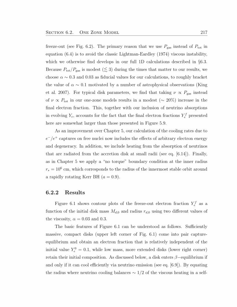
Section 6.2. One Zone Model 217
freeze-out (see Fig. 6.2). The primary reason that we use Pgas instead of Ptot in
equation (6.4) is to avoid the classic Lightman-Eardley (1974) viscous instability,
which we otherwise find develops in our full 1D calculations described in §6.3.
Because Ptot/Pgas is modest (. 3) during the times that matter to our results, we
choose α ∼ 0.3 and 0.03 as fiducial values for our calculations, to roughly bracket
the value of α ∼ 0.1 motivated by a number of astrophysical observations (King
et al. 2007). For typical disk parameters, we find that taking ν ∝ Pgas instead
of ν ∝ Ptot in our one-zone models results in a modest (∼ 20%) increase in the
final electron fraction. This, together with our inclusion of neutrino absorptions
in evolving Ye, accounts for the fact that the final electron fractions Y fe presented
here are somewhat larger than those presented in Figure 5.9.
As an improvement over Chapter 5, our calculation of the cooling rates due to
e−/e+ captures on free nuclei now includes the effects of arbitrary electron energy
and degeneracy. In addition, we include heating from the absorption of neutrinos
that are radiated from the accretion disk at small radii (see eq. [6.14]). Finally,
as in Chapter 5 we apply a “no torque” boundary condition at the inner radius
r∗ = 106 cm, which corresponds to the radius of the innermost stable orbit around
a rapidly rotating Kerr BH (a = 0.9).
6.2.2 Results
Figure 6.1 shows contour plots of the freeze-out electron fraction Y fe as a
function of the initial disk mass Md,0 and radius rd,0 using two different values of
the viscosity, α = 0.03 and 0.3.
The basic features of Figure 6.1 can be understood as follows. Sufficiently
massive, compact disks (upper left corner of Fig. 6.1) come into pair capture-
equilibrium and obtain an electron fraction that is relatively independent of the
initial value Y 0e = 0.1, while low mass, more extended disks (lower right corner)
retain their initial composition. As discussed below, a disk enters β−equilibrium if
and only if it can cool efficiently via neutrino emission (see eq. [6.9]). By equating
the radius where neutrino cooling balances ∼ 1/2 of the viscous heating in a self-
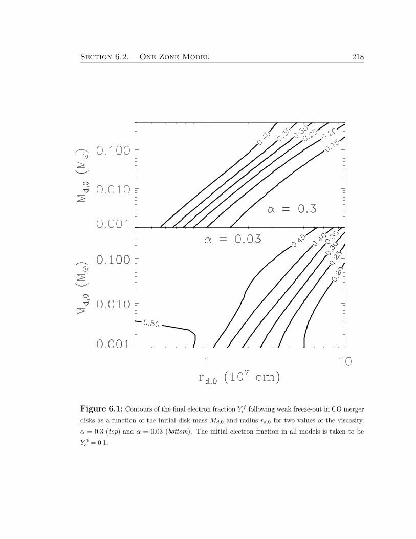
Section 6.2. One Zone Model 218
Figure 6.1: Contours of the final electron fraction Y fe following weak freeze-out in CO merger
disks as a function of the initial disk mass Md,0 and radius rd,0 for two values of the viscosity,
α = 0.3 (top) and α = 0.03 (bottom). The initial electron fraction in all models is taken to be
Y 0e = 0.1.
Section 6.2. One Zone Model 219
0.01 0.10 1.00Time (s)
0.1
1.0
0.01 0.10 1.00Time (s)
0.1
1.0
10.0
Rat
es (
t vis
c-1)
Figure 6.2: The process of weak freeze-out in our one-zone model of a viscously-spreading,
hyper-accreting disk. The left panel shows the time evolution of the electron fraction Ye (solid
line), disk thickness H/rd (dashed line), degeneracy parameter µe/kT (triple-dot-dashed line),
and the ratio of gas to total pressure Pgas/Ptot (dot-dashed line), calculated for α = 0.3 and for a
disk with initial massMd,0 = 0.1M¯ and radius rd,0 = 3×106 cm. Also shown with a dotted line
is the equilibrium electron fraction Y eqe obtained by setting the right hand side of equation (6.2)
to zero. The right panel shows the rates of the weak interactions that modify Ye(t), normalized
to the viscous timescale tvisc. The electron, positron, and neutrino capture rates are denoted by
λep, λe+n, and λνN , respectively. Note that Ye freezes out of equilibrium at the same time that
the disk becomes advective (H/rd & 0.5) and non-degenerate (µe . kT ). Since Y eqe rises to & 0.5
as the disk becomes non-degenerate, the final composition is only moderately neutron-rich, with
a final electron fraction Y fe ' 0.43.
Section 6.2. One Zone Model 220
similar solution for a thick disk, we estimate analytically that disks that satisfy
Md,0 & 3× 10⁻³( rd,0107cm
)7/3 ( α
0.1
)2/3
M¯ (6.5)
are sufficiently compact to become neutrino-cooled and neutron-rich at early stages
in their evolution (see also eq. [5.19] and surrounding discussion). Equation (6.5)
does a reasonable job of reproducing the parameter space in Figure 6.1 where Y fe
differs significantly from its initial value. For instance, equation (6.5) shows that
lower values of α allow less massive disks of a fixed size to enter β-equilibrium;
this is consistent with the wider parameter space with Y fe > Y 0
e = 0.1 at low α.
To illustrate the process of weak freeze-out explicitly, Figure 6.2 (left panel)
shows the evolution of the electron fraction Ye(t) for a disk withMd,0 = 0.1M¯ and
rd,0 = 3 × 106 cm. We also show the equilibrium electron fraction Y eqe (obtained
by setting the right hand side of eq. [6.2] to zero), the ratio of the disk scaleheight
to the radius H/rd, the ratio of the gas pressure to the total pressure Pgas/Ptot,
and the ratio of the electron chemical potential to the disk temperature µe/kT
(i.e., the degeneracy parameter). Also shown for comparison in the right panel of
Figure 6.2 are the weak interaction rates from equation (6.2), normalized to the
viscous timescale tvisc ≡ α−1Ω−1(H/rd)−2.
Figure 6.2 shows that at early times, when the disk is neutrino-cooled and
H/rd ∼ 1/3, pair captures are rapid compared to the viscous timescale. Thus,
the disk enters β−equilibrium with an electron fraction Ye ≈ Y eqe that is ¿ 0.5
because positron captures are suppressed relative to electron captures under the
degenerate conditions (µe À kT ) in the midplane. At later times (t ∼ 0.1 s) the
disk thickens to H/rd ∼ 0.5 and becomes non-degenerate (µe ¿ kT ) and radiation
pressure-dominated. At this point Y eqe rises to & 0.5 because positron captures
under non-degenerate conditions now become energetically favored over electron
captures due to the proton-neutron mass difference. Note, however, that as the
disk thickens weak interactions become slow compared to the viscous timescale and
Ye freezes out at the value Y fe ≈ 0.43. Although (non-local) neutrino absorptions
are unimportant relative to electron captures at early times, their rate λνN is
comparable to the pair capture rates near freeze-out and must be included to
Section 6.2. One Zone Model 221
accurately determine Y fe .
Figure 6.1 shows that moderately neutron-rich freeze-out (Y fe ∼ 0.3− 0.5) is
a common feature of accretion disks formed from CO mergers for a wide range of
initial conditions. However, contrasting the disk’s neutron-rich equilibrium state
(Ye ' Y eqe ∼ 0.1) at early times with its final, non-degenerate state that actually
favors a proton-rich composition in equilibrium (i.e., Y eqe > 0.5), it is a priori
unclear why Ye freezes out with a value Y fe ∼ 0.3−0.5 between these two extremes.
To understand why this is the case, note that an approximate condition for
weak freeze-out is that the pair capture timescale becomes longer than the viscous
time tvisc. Since the disk becomes non-degenerate around freeze-out, electron and
positron captures occur at a similar rate (e.g., Qian & Woosley 1996)
λeN ≈ 0.45T 5MeV s−1, (6.6)
where T ≡ TMeVMeV and eN represents either e−p or e+n. The associated URCA
cooling rate per nucleon is given by
QeN = 〈εν〉λeN ≈ 2.3T 6MeV MeV s−1, (6.7)
where 〈εν〉 ≈ 5.04kT is the mean neutrino energy released per capture. The viscous
heating rate per nucleon at r À r∗ is
Qvisc =9
4νΩ2mN ≈
9
4αmNr
2Ω3
(
H
r
)2
, (6.8)
wheremN is the nucleon mass. If we assume that the disk is supported primarily by
gas pressure3 then the midplane temperature is kT ≈ mNr2Ω2(H/r)2. Combining
this with equations (6.6)− (6.8) we find that
λeN tvisc =9
4
(
kT
〈εν〉
)(
H
r
)−2(
QeN
Qvisc
)
' 1.8
(
QeN
Qvisc
)
(
H/r
0.5
)−2
. (6.9)
Equation (6.9) shows that once neutrino cooling no longer offsets viscous heat-
ing (i.e., Qvisc & QeN) and the disk thickens to H/r ∼ 1, weak freeze-out (i.e.,
3As discussed in §6.2.1 and shown in Figure 6.2, gas and radiation pressure are comparableat freeze-out; the assumption that gas pressure dominates is, however, sufficient for the purposesof a simple estimate.
Section 6.3. Height-Integrated Model 222
λeN tvisc . 1) necessarily results. Physically, this occurs because the disk is cooled
by e−/e+ captures, the very same processes that largely control the evolution of
Ye (see Fig. 6.2). This conclusion is fairly robust because it applies at any radius
and is independent of the value of α. Although the absorption of neutrinos from
the central disk threatens to complicate this simple argument, the right panel of
Figure 6.2 shows that the effect of absorptions is at most comparable to that of
pair captures prior to freeze-out.
6.3 Height-Integrated Model
The results of §6.2 suggest that neutron-rich freeze-out is a common feature
of viscously-spreading, hyper-accreting disks. However, the one-zone model makes
a number of simplifying assumption that may affect the final electron fraction Y fe .
In this section we present a 1D (height-integrated) model of a viscously-spreading
disk that more precisely determines Y fe and its distribution with mass. In §6.3.1
we describe the initial conditions and relevant equations. Then we present our
results in §6.3.2.
6.3.1 Equations and Initial Conditions
Our 1D calculation evolves the surface density Σ, midplane temperature T ,
and electron fraction Ye as a function of radius r and time t using the 2N-RK3
(6th order space, 3rd order time) scheme described in Brandenburg (2001). We
use a logarithmic radial grid that extends from just outside the inner edge of the
disk at r∗ = 106 cm, out to a radius that safely exceeds the outer edge of the disk
at the final time step (typically ≈ 109 cm).
The surface density is evolved according to the diffusion equation for an ax-
isymmetric disk in a Newtonian 1/r gravitational potential (e.g., Frank et al. 2002):
∂Σ
∂t=
3
r
∂
∂r
[
r1/2∂
∂r
(
νΣr1/2)
]
, (6.10)
where the viscosity ν is proportional to just the gas pressure (see eq. [6.4] and
Section 6.3. Height-Integrated Model 223
surrounding discussion). The radial velocity vr is not evolved explicitly but instead
follows from equation (6.10) and mass continuity:
vr =−3
Σr1/2∂
∂r
(
νΣr1/2)
. (6.11)
We take the initial surface density of the disk to be
Σ(r, t = 0) ∝
(
r
rd,0
)m
exp
[
−(2 +m)
(
r
rd,0
)]
, (6.12)
with the constant of proportionality set by requiring that the total disk mass equals
Md,0. Equation (6.12) concentrates the initial disk mass ∝ Σr2 about the radius
rd,0, with larger values of the parameter m resulting in a more narrowly concen-
trated mass distribution. As discussed in §6.2.1, the precise mass distribution of
disks produced from CO mergers is uncertain theoretically. In most of our calcu-
lations we take m = 5, although our results are relatively insensitive to m. Due to
numerical issues that arise from the exponential drop-off of Σ at the outer edge of
the disk, we impose an initial density floor that is sufficiently small that matter at
the density floor contains a fraction . 10−3 of the total disk mass at any time; we
have verified that our results are insensitive to the level of this floor as long as it
contains negligible mass. We have also performed calculations using a power-law
density distribution that concentrates the disk’s initial mass at small radii (e.g.,
Σ ∝ r−3); we find results that are similar to those obtained using equation (6.12)
with rd,0 taken near the disk’s inner edge.
We calculate the scaleheight H by assuming hydrostatic equilibrium in the
vertical direction, i.e., we take H = cs/Ω, where cs ≡ (Ptot/ρ)1/2 is the isothermal
sound speed. We evolve the midplane temperature using the equation for the
specific entropy S, which is given by
TdS
dt= qvisc − q
−ν + q+ν , (6.13)
where (d/dt) ≡ (∂/∂t)+vr(∂/∂r), qvisc = (9/4)νΩ2 is the viscous heating rate, and
q−ν is the neutrino cooling rate, as given in Di Matteo et al. (2002) but modified
to include the effects of arbitrary Ye and electron degeneracy (e.g., Beloborodov
Section 6.3. Height-Integrated Model 224
2003). The term
q+ν = λνep〈ενe〉
[
Ye −
(
1−Xf
2
)]
+ λνen〈ενe〉
[
1− Ye −
(
1−Xf
2
)]
(6.14)
represents neutrino heating from the inner radii of the accretion disk, where λνen
and λνep are the neutrino capture rates given by equation (6.3). We not not
include heating due to α−particle formation because we are primarily interested
in determining the final electron fraction, and α−particles form only after the disk
has fallen out of weak equilibrium.
The initial temperature profile is set by requiring that H/r = 0.3 at all radii.
An initially thick disk is physically motivated by the fact that CO merger disks
form dynamically hot; however, because the thermal time is short compared to
the viscous time, the disk’s evolution quickly becomes independent of the initial
scaleheight anyways.
Finally, we evolve the electron fraction profile Ye(r) using equation (6.2), with
d/dt = ∂/∂t + vr∂/∂r. To keep the required timesteps reasonable, we equate Ye
with its equilibrium value Y eqe when the weak interaction rates greatly exceed the
local viscous rate 1/tvisc. As in §6.2, we take the initial electron fraction to be
Y 0e = 0.1 at all radii.
The surface density across the ghost zones at the inner boundary is set to
enforce a constant mass accretion rate M ∝ Σν at the value of M in the first
active zone. We interpolate the temperature and electron fraction at the inner
boundary. Unlike in the one-zone calculations in §6.2, we do not implement a
no-torque boundary condition on the inner edge of the disk, in part because it
leads to an unphysical temperature profile at small radii (in particular, T → 0
as r → r∗). Our results for Y fe are not sensitive to this boundary condition. We
also interpolate all variables at the outer boundary, although this choice has no
effect on our results because the outer boundary is not in causal contact with the
inner flow. We have verified that our code conserves total mass Mtot and angular
momentum J by checking that decreases inMtot and J with time are compensated
by their fluxes across the inner grid cell.
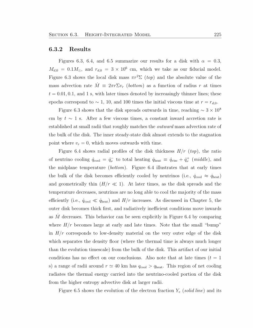
Section 6.3. Height-Integrated Model 225
6.3.2 Results
Figures 6.3, 6.4, and 6.5 summarize our results for a disk with α = 0.3,
Md,0 = 0.1M¯, and rd,0 = 3 × 106 cm, which we take as our fiducial model.
Figure 6.3 shows the local disk mass πr2Σ (top) and the absolute value of the
mass advection rate M ≡ 2πrΣvr (bottom) as a function of radius r at times
t = 0.01, 0.1, and 1 s, with later times denoted by increasingly thinner lines; these
epochs correspond to ∼ 1, 10, and 100 times the initial viscous time at r = rd,0.
Figure 6.3 shows that the disk spreads outwards in time, reaching ∼ 3 × 10⁸
cm by t ∼ 1 s. After a few viscous times, a constant inward accretion rate is
established at small radii that roughly matches the outward mass advection rate of
the bulk of the disk. The inner steady-state disk almost extends to the stagnation
point where vr = 0, which moves outwards with time.
Figure 6.4 shows radial profiles of the disk thickness H/r (top), the ratio
of neutrino cooling qcool = q−ν to total heating qheat ≡ qvisc + q+ν (middle), and
the midplane temperature (bottom). Figure 6.4 illustrates that at early times
the bulk of the disk becomes efficiently cooled by neutrinos (i.e., qcool ≈ qheat)
and geometrically thin (H/r ¿ 1). At later times, as the disk spreads and the
temperature decreases, neutrinos are no long able to cool the majority of the mass
efficiently (i.e., qcool ¿ qheat) and H/r increases. As discussed in Chapter 5, the
outer disk becomes thick first, and radiatively inefficient conditions move inwards
as M decreases. This behavior can be seen explicitly in Figure 6.4 by comparing
where H/r becomes large at early and late times. Note that the small “bump”
in H/r corresponds to low-density material on the very outer edge of the disk
which separates the density floor (where the thermal time is always much longer
than the evolution timescale) from the bulk of the disk. This artifact of our initial
conditions has no effect on our conclusions. Also note that at late times (t = 1
s) a range of radii around r ' 40 km has qcool > qheat. This region of net cooling
radiates the thermal energy carried into the neutrino-cooled portion of the disk
from the higher entropy advective disk at larger radii.
Figure 6.5 shows the evolution of the electron fraction Ye (solid line) and its
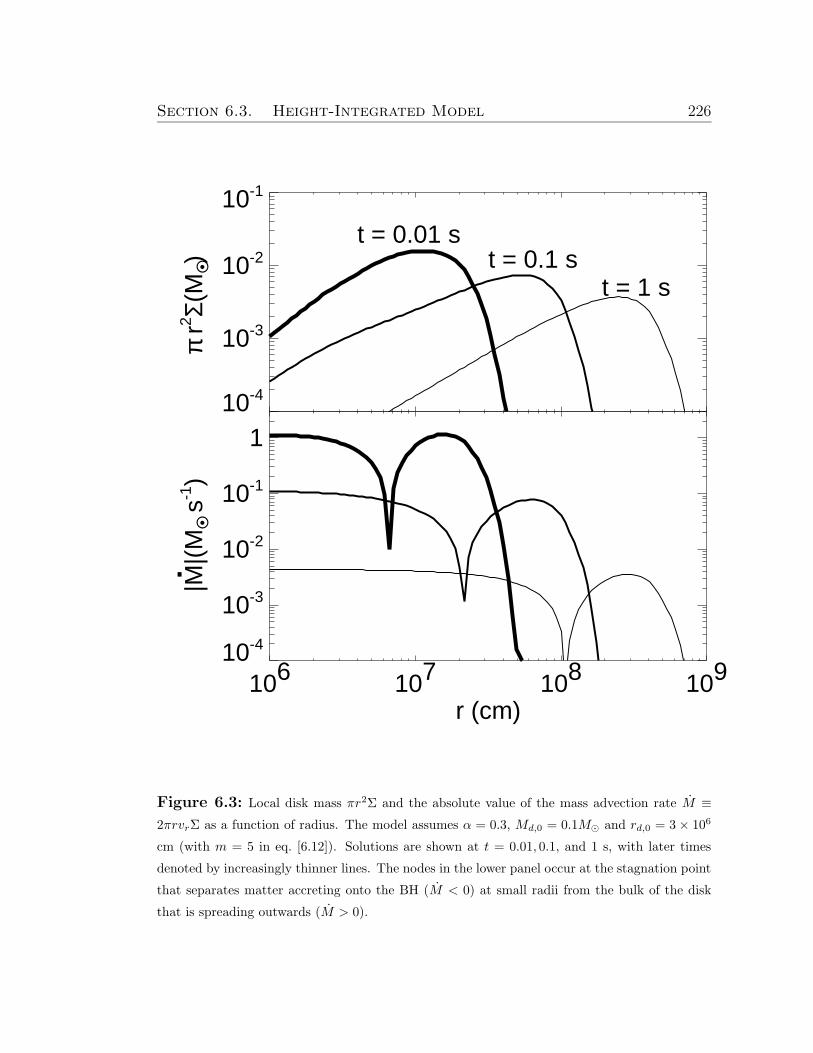
Section 6.3. Height-Integrated Model 226
10-4
10-3
10-2
10-1π
r2 Σ(M
O •)
106 107 108 109
r (cm)
10-4
10-3
10-2
10-1
1
|M|(
MO • s
-1)
.
t = 0.01 st = 0.1 s
t = 1 s
Figure 6.3: Local disk mass πr2Σ and the absolute value of the mass advection rate M ≡
2πrvrΣ as a function of radius. The model assumes α = 0.3, Md,0 = 0.1M¯ and rd,0 = 3× 10⁶
cm (with m = 5 in eq. [6.12]). Solutions are shown at t = 0.01, 0.1, and 1 s, with later times
denoted by increasingly thinner lines. The nodes in the lower panel occur at the stagnation point
that separates matter accreting onto the BH (M < 0) at small radii from the bulk of the disk
that is spreading outwards (M > 0).
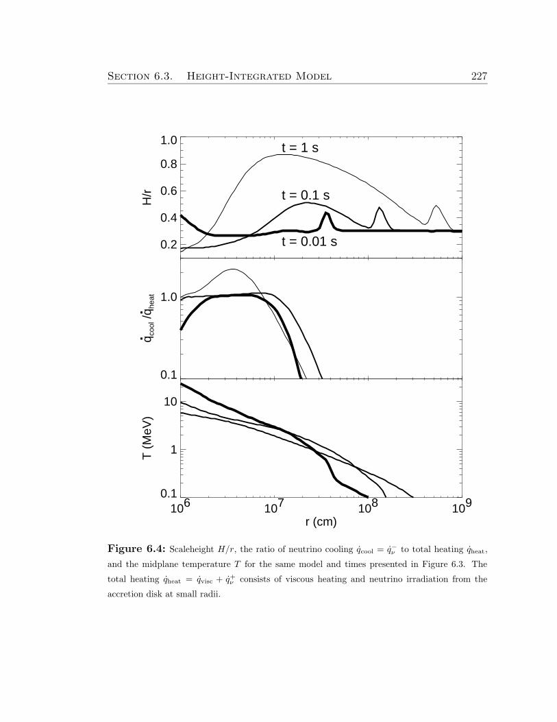
Section 6.3. Height-Integrated Model 227
106 107 108 109
r (cm)
0.1
1
10
T (
MeV
)
0.2
0.4
0.6
0.8
1.0H
/rt = 1 s
t = 0.1 s
t = 0.01 s
0.1
1.0
q coo
l /q h
eat
.
.
Figure 6.4: Scaleheight H/r, the ratio of neutrino cooling qcool = q−ν to total heating qheat,
and the midplane temperature T for the same model and times presented in Figure 6.3. The
total heating qheat = qvisc + q+ν consists of viscous heating and neutrino irradiation from the
accretion disk at small radii.
Section 6.3. Height-Integrated Model 228
106 107 108 109
r (cm)
0.2
0.4
0.6
0.8
Ele
ctro
n F
ract
ion
Ye
Yeeq
t = 0.01 s
t = 0.1 s
t = 1 s
Figure 6.5: Electron fraction Ye (solid line) and the equilibrium electron fraction Y eqe
(dotted line) for the same model and times presented in Figures 6.3 and 6.4. At early times,
the disk is in β−equilibrium, with Ye ≈ Y eqe ¿ 0.5 at all radii that contain substantial mass. At
later times, Y eqe rises as the disk becomes advective and non-degenerate, and Ye freezes out with
final values in the range Y fe ∼ 0.1− 0.5 (see Fig. 6.7).
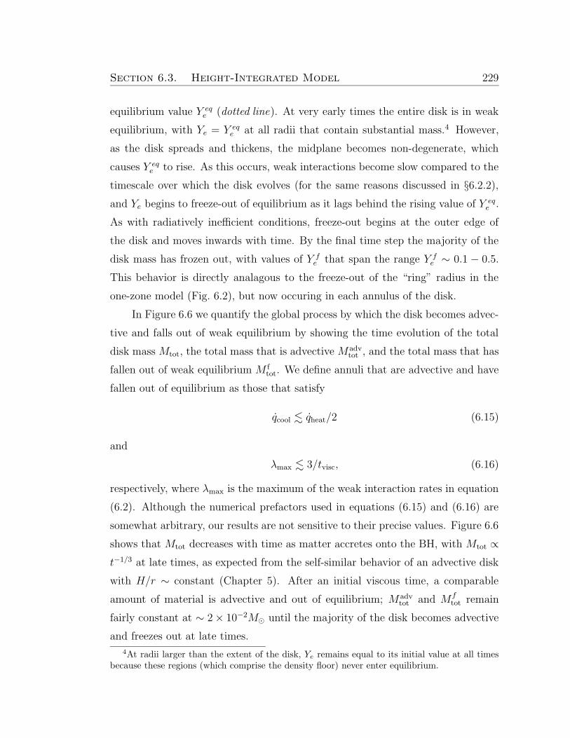
Section 6.3. Height-Integrated Model 229
equilibrium value Y eqe (dotted line). At very early times the entire disk is in weak
equilibrium, with Ye = Y eqe at all radii that contain substantial mass.4 However,
as the disk spreads and thickens, the midplane becomes non-degenerate, which
causes Y eqe to rise. As this occurs, weak interactions become slow compared to the
timescale over which the disk evolves (for the same reasons discussed in §6.2.2),
and Ye begins to freeze-out of equilibrium as it lags behind the rising value of Y eqe .
As with radiatively inefficient conditions, freeze-out begins at the outer edge of
the disk and moves inwards with time. By the final time step the majority of the
disk mass has frozen out, with values of Y fe that span the range Y f
e ∼ 0.1 − 0.5.
This behavior is directly analagous to the freeze-out of the “ring” radius in the
one-zone model (Fig. 6.2), but now occuring in each annulus of the disk.
In Figure 6.6 we quantify the global process by which the disk becomes advec-
tive and falls out of weak equilibrium by showing the time evolution of the total
disk mass Mtot, the total mass that is advective M advtot , and the total mass that has
fallen out of weak equilibrium M ftot. We define annuli that are advective and have
fallen out of equilibrium as those that satisfy
qcool . qheat/2 (6.15)
and
λmax . 3/tvisc, (6.16)
respectively, where λmax is the maximum of the weak interaction rates in equation
(6.2). Although the numerical prefactors used in equations (6.15) and (6.16) are
somewhat arbitrary, our results are not sensitive to their precise values. Figure 6.6
shows that Mtot decreases with time as matter accretes onto the BH, with Mtot ∝
t−1/3 at late times, as expected from the self-similar behavior of an advective disk
with H/r ∼ constant (Chapter 5). After an initial viscous time, a comparable
amount of material is advective and out of equilibrium; M advtot and M f
tot remain
fairly constant at ∼ 2× 10⁻²M¯ until the majority of the disk becomes advective
and freezes out at late times.
4At radii larger than the extent of the disk, Ye remains equal to its initial value at all timesbecause these regions (which comprise the density floor) never enter equilibrium.
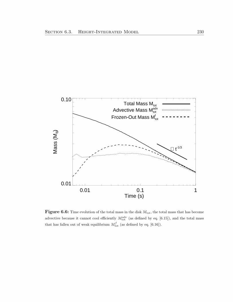
Section 6.3. Height-Integrated Model 230
0.01 0.1 1Time (s)
0.01
0.10
Mas
s (M
O •)
∝ t-1/3
Total Mass Mtot
Advective Mass Mtotadv
Frozen-Out Mass Mtotf
Figure 6.6: Time evolution of the total mass in the diskMtot, the total mass that has become
advective because it cannot cool efficiently M advtot (as defined by eq. [6.15]), and the total mass
that has fallen out of weak equilibrium M ftot (as defined by eq. [6.16]).
Section 6.3. Height-Integrated Model 231
0.001
0.010
M(Y
e) (
MO • b
in-1)
0.1 0.2 0.3 0.4 0.5 0.6Ye
0.001
0.010
M(Y
e) (
MO • b
in-1)
t = 1.3 s
t = 8 s
Figure 6.7: Amount of mass with a given electron fraction M(Ye) for the model with Md,0 =
0.1M¯, rd,0 = 3×106 cm, and α = 0.3. The solid and dotted lines include, respectively, mass that
has become advective (eq. [6.15]) and that has fallen out of weak equilibrium (eq. [6.16]). The
times t = 0.03 s and 0.3 s correspond to when the disk is 50% and 90% advective, respectively.
Section 6.3. Height-Integrated Model 232
As discussed in §6.1, once a portion of the disk becomes advective, a viscously-
driven outflow likely drives away a substantial portion of its mass (e.g., Blandford
& Begelman 1999). In our calculations we have neglected the effects of such a mass
sink on the evolution of the disk. Figure 6.6 shows that this approximation remains
reasonable until t ∼ 0.03 − 0.1 s because prior to this point the majority of the
disk remains neutrino cooled. Mass- and angular momentum-loss to a wind leads
to a more rapid decline in M , which further speeds up the onset of the advective
phase and weak freeze-out at smaller radii (Chapter 5).
In Figure 6.7 we show histograms of mass as a function of electron fraction
M(Ye) at the times t = 0.03 s and t = 0.3 s. The solid and dashed lines are
the matter that is advective and out of β−equilibrium, respectively (as defined by
eqs. [6.15] and [6.16]). These distributions typically correspond to the same matter
because annuli fall out of equilibrium as they become advective (see eq. [6.9]). We
show the composition at these two particular times because they correspond to
epochs when the disk has become≈ 50% and 90% advective, respectively (Fig. 6.6).
Thus, these distributions likely represent typical values of the electron fraction in
the viscously-driven outflows that dominate subsequent mass-loss from the disk.
It is useful to compare the results in Figure 6.7 with the one zone calculation
from §6.2 for the same initial disk parameters (see Fig. 6.1). When the disk is
90% advective at t = 0.3 s, the height-integrated calculation finds a final electron
fraction distribution centered around a mass-averaged value 〈Y fe 〉 ≈ 0.29, which is
somewhat lower than the value of Y fe = 0.43 given by the one-zone model. Indeed,
in most of our calculations we find that Y fe calculated using the one zone model
tends to slightly exceed 〈Y fe 〉 obtained from the full 1D calculations.
In Figures 6.8 and 6.9 we show histograms similar to Figure 6.7, but for
solutions calculated with a lower viscosity (α = 0.03) and a lower initial mass
(Md,0 = 0.01M¯), respectively. The times chosen correspond to epochs when the
disk is 50% and 90% advective. The mass-averaged electron fraction when the disk
is 90% advective is 〈Y fe 〉 ≈ 0.3 for both the lower α and lower Md,0 models. The
similarity in the distribution of Y fe for α = 0.3 and α = 0.03 in Figures 6.7 and
6.8 supports our argument that the freeze-out process is relatively independent of
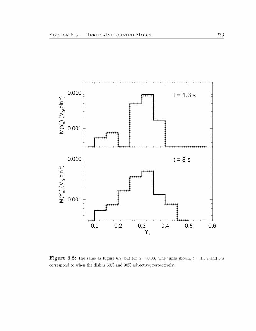
Section 6.3. Height-Integrated Model 233
0.001
0.010
M(Y
e) (
MO • b
in-1)
0.1 0.2 0.3 0.4 0.5 0.6Ye
0.001
0.010
M(Y
e) (
MO • b
in-1)
t = 1.3 s
t = 8 s
Figure 6.8: The same as Figure 6.7, but for α = 0.03. The times shown, t = 1.3 s and 8 s
correspond to when the disk is 50% and 90% advective, respectively.
Section 6.4. Discussion 234
the details of how the disk viscously spreads (see §6.2.2). The lower disk mass
case (Fig. 6.9) is notable because a significant fraction of the disk’s mass freezes
out with Ye . 0.2, and such low-Ye material may produce third-peak r-process
elements (Hoffman et al. 1997).
We have performed freeze-out calculations for a number of other disk param-
eters. In Table 6.1 we summarize our results for 〈Y fe 〉 and the fraction fadv of the
initial disk mass that remains when the disk is 90% advective. Although different
initial mass distributions and viscosities give somewhat different Y fe distributions,
the neutron-rich freeze-out of ∼ 20 − 50% of the disk’s original mass is a generic
property of the disks created during CO mergers.
6.4 Discussion
Accretion disks formed from CO mergers that are sufficiently massive and
compact to satisfy equation (6.5) become neutrino-cooled, degenerate, and neutron-
rich early in their evolution. Eventually, as the disk accretes and viscously spreads,
neutrino cooling is no longer able to offset viscous heating and the disk becomes
advective. At this point several important changes occur nearly simultaneously:
the disk becomes geometrically thick (H/r ∼ 1), radiation pressure-dominated,
and non-degenerate at the same time that the equilibrium electron fraction Y eqe
rises from¿ 0.5 to & 0.5 and Ye freezes out (Fig. 6.2; see also Beloborodov 2008).
Weak freeze-out necessarily accompanies the disk’s advective transition because
e−/e+ captures are primarily responsible for both cooling the disk and setting its
electron fraction (see eq. [6.9] of §6.2.2). Because Y eqe is rising as freeze-out occurs,
moderately neutron-rich freeze-out with Y fe ≈ 0.2− 0.4 is a generic feature of ac-
cretion disks formed from CO mergers. Our calculations in §6.2 and §6.3 largely
confirm this basic conclusion (see Table 6.1).
Neutron-rich freeze-out in hyper-accreting disks is usefully contrasted with
the proton−rich freeze-out (Y fe ' 0.88) in the very early universe. Big bang
nucleosynthesis (BBN) occurred on a timescale of minutes under non-degenerate
and highly radiation-dominated conditions (entropy S ∼ 1010 kB baryon−1). By
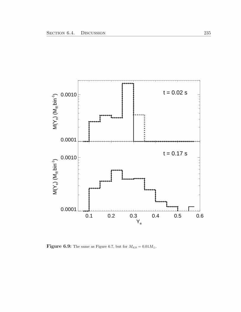
Section 6.4. Discussion 235
0.0001
0.0010
M(Y
e) (
MO • b
in-1)
0.1 0.2 0.3 0.4 0.5 0.6Ye
0.0001
0.0010
M(Y
e) (
MO • b
in-1)
t = 0.02 s
t = 0.17 s
Figure 6.9: The same as Figure 6.7, but for Md,0 = 0.01M¯.
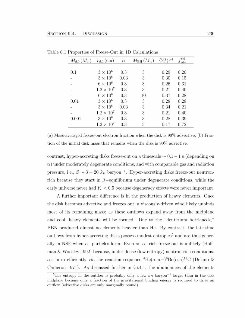
Section 6.4. Discussion 236
Table 6.1 Properties of Freeze-Out in 1D Calculations
Md,0 (M¯) rd,0 (cm) α MBH (M¯) 〈Y fe 〉
(a) f(b)adv
0.1 3× 10⁶ 0.3 3 0.29 0.20- 3× 10⁶ 0.03 3 0.30 0.15- 6× 10⁶ 0.3 3 0.26 0.31- 1.2× 10⁷ 0.3 3 0.21 0.40- 6× 10⁶ 0.3 10 0.37 0.280.01 3× 10⁶ 0.3 3 0.28 0.28- 3× 10⁶ 0.03 3 0.34 0.21- 1.2× 10⁷ 0.3 3 0.21 0.400.001 3× 10⁶ 0.3 3 0.28 0.39- 1.2× 10⁷ 0.3 3 0.17 0.72
(a) Mass-averaged freeze-out electron fraction when the disk is 90% advective; (b) Frac-
tion of the initial disk mass that remains when the disk is 90% advective.
contrast, hyper-accreting disks freeze-out on a timescale ∼ 0.1−1 s (depending on
α) under moderately degenerate conditions, and with comparable gas and radiation
pressure, i.e., S ∼ 3− 20 kB baryon−1. Hyper-accreting disks freeze-out neutron-
rich because they start in β−equilibrium under degenerate conditions, while the
early universe never had Ye < 0.5 because degeneracy effects were never important.
A further important difference is in the production of heavy elements. Once
the disk becomes advective and freezes out, a viscously-driven wind likely unbinds
most of its remaining mass; as these outflows expand away from the midplane
and cool, heavy elements will be formed. Due to the “deuterium bottleneck,”
BBN produced almost no elements heavier than He. By contrast, the late-time
outflows from hyper-accreting disks possess modest entropies5 and are thus gener-
ally in NSE when α−particles form. Even an α−rich freeze-out is unlikely (Hoff-
man & Woosley 1992) because, under dense (low entropy) neutron-rich conditions,
α’s burn efficiently via the reaction sequence 4He(α n,γ)9Be(α,n)12C (Delano &
Cameron 1971). As discussed further in §6.4.1, the abundances of the elements
5The entropy in the outflow is probably only a few kB baryon−1 larger than in the diskmidplane because only a fraction of the gravitational binding energy is required to drive anoutflow (advective disks are only marginally bound).
Section 6.4. Discussion 237
synthesized are thus approximately determined by neutron-rich NSE (Hartmann
et al. 1985).
It is also important to contrast the site of nucleosynthesis that we have intro-
duced here with outflows driven from the disk by neutrino heating (e.g., Levinson
2006; Barzilay & Levison 2008; Chapter 4). Neutrino-driven outflows generally oc-
cur at early times or small radii, when the disk midplane is still in β−equilibrium
and the irradiating neutrino flux is substantial. The outflow’s final electron frac-
tion in this case is set by an equilibrium with neutrino absorptions (Ye ≈ Y νe
in eq. [6.1]) and is not directly related to Ye in the midplane (e.g., Surman &
McLaughlin 2004). By contrast, the outflows considered here occur after the mid-
plane itself has fallen out of weak equilibrium, and so the disk’s electron fraction
Y fe is retained by the outflow. While neutrino absorptions in the disk are some-
what important near freeze-out, at no point does the midplane electron fraction
enter equilibrium with the neutrinos, as generically occurs in neutrino-driven out-
flows (Chapter 4). Instead, the outwardly-spreading disk provides a protective
“cocoon” that transports low-Ye material (kept neutron-rich by degenerate elec-
tron capture) away from the deneutronizing flux of neutrinos from the central disk.
Furthermore, the viscously-driven outflows that we have focused on carry away a
substantial fraction of the disk’s initial mass; because neutrino-driven outflows
likely eject less mass (Chapter 5), the total nucleosynthetic yield from CO mergers
is probably dominated by the viscously-driven outflows at late times.
Finally, although we believe that the disk is largely unbound by viscous heat-
ing once it becomes advective (Blandford & Begelman 1999; Stone & Pringle
2001), if nothing else the energy released by α−particle (or even heavier element)
formation is sufficient to unbind the disk at late times (Lee & Ramirez-Ruiz 2007;
Chapter 5). Since α−particle formation occurs soon after the disk becomes ad-
vective, our conclusions would be qualitatively unchanged if nuclear (rather than
viscous) energy powers the late-time outflow. In this case the formation of heavy
elements would begin in the disk midplane, but the final nucleosynthetic yield
would probably be similar.
Section 6.4. Discussion 238
6.4.1 Implications
As we have argued, moderate entropy, neutron-rich outflows appear to be a
common property of accretion disks formed from CO mergers at late times. Al-
though detailed calculations of the dynamics and nucleosynthesis in these outflows
need to be performed, the late-time conditions in the disk favor the production
of elements with abundances close to their NSE values at charged-particle reac-
tion freeze-out. In particular, the entropies (∼ 10 kB baryon−1) and dynamical
timescales (τdyn ∼ 0.01 − 0.1 s) at freeze-out are similar to those explored in low
entropy nucleosynthesis calculations by Woosley & Hoffman (1992). For example,
in their model with S ≈ 29 kB baryon−1 and τdyn ≈ 0.1 s, these authors find
that all α−particles reassemble into heavy nuclei for Ye . 0.45, and that the final
abundances closely resemble those of NSE (see the second column in their Table
2).
Neutron-rich NSE calculations were performed by Hartmann et al. (1985).
For Ye ≈ 0.35 − 0.40, they find that the predominant isotopes created are 82Se,
79Br, and 78Se (in order of decreasing Ye; see their Fig. 3). The very low solar
system abundances of these isotopes (total mass fraction X¯ ≈ 3× 10⁻⁸) strongly
constrains the rate of astrophysical events that produce material with Ye ≈ 0.35−
0.4 in NSE: we estimate that the maximum allowed mass ejection of material with
Ye ≈ 0.35 − 0.4 into the ISM is Mmax ≈ (MgalX¯/tgal) ≈ 1.5 × 10⁻⁷M¯ yr−1,
where tgal ≈ 1010 yrs and Mgal ≈ 5×10¹⁰M¯ and are the age and baryonic mass of
the Galaxy, respectively (Binney & Tremaine 1994). More neutron-rich material
(Ye . 0.35) will produce even heavier isotopes and, possibly, an r-process. Since
these elements are also very rare, a similar constraint can be placed on the rate
that very low-Ye material is ejected into the ISM. For instance, isotopes near the
second r-process peak (A ∼ 130) have a typical solar mass abundance X r¯ ∼ 10−9
relative to hydrogen; therefore, if material ejected with 0.2 . Ye . 0.35 produced
equal numbers of N ∼ 10 r-process isotopes in this mass range, the constraint on
the mass ejected would be Mmax ∼ 5 × 10⁻⁸(N/10)M¯ yr−1, comparable to the
rate for material with Ye ≈ 0.35 − 0.4 given above. In order to be conservative,
Section 6.4. Discussion 239
below we use the constraint Mmax ≈ 1.5 × 10⁻⁷M¯ yr−1 for all material ejected
with Ye . 0.4. However, a more precise determination of the isotopes produced by
the ejection of moderate entropy material with Ye ≈ 0.2− 0.35 would likely place
even stronger constraints on the rate of CO mergers.
Based on Figures 6.7-6.9 and our one-zone calculations in §6.2 we find that
a fraction fadv ≈ 0.2 − 0.5 of the disk’s initial mass remains when it becomes
advective at late times (see Table 6.1), with a higher fraction for less massive,
more extended disks. Of this material, we estimate that the majority of the mass
will have Y fe . 0.4, when averaging over many events with different initial disk
properties (see Figs. 6.7-6.9 and Table 6.1). Although ejecta from mergers that
occur outside Galactic disk will not enrich the ISM, population synthesis studies
estimate that for large spirals such as the Milky Way only a small fraction (. 20%)
of mergers occur in intergalactic space (Belczynski et al. 2006). Thus a fraction
η ≈ 0.1 − 0.5 of the disk’s initial mass will both become unbound from the disk
and pollute the ISM with rare neutron-rich isotopes. Hence, if the average mass of
the disks formed from CO mergers is 〈Md,0〉, their rate in the Milky Way cannot
exceed
Nmax ≈Mmax
η〈Md,0〉≈ 10−5
( η
0.2
)−1(
〈Md,0〉
0.1M¯
)−1
yr−1, (6.17)
where we have normalized η to a typical value ∼ 0.2.
Based on observed binary NS systems, Kalogera et al. (2004) find that the
NS-NS merger rate in the Milky Way is between 1.7 × 10⁻⁵ and 2.9 × 10⁻⁴ yr−1
at 95% confidence. Population synthesis estimates (e.g., Belczynski et al. 2006)
are consistent with this range but with larger uncertainties. Our constraint in
equation (6.17) thus requires either NS-NS merger rates at the low end of current
estimates, or a small average disk mass ¿ 0.1M¯.
Ultimately, equation (6.17) must be combined with GR simulations of the
merger process that determine Md,0 as a function of the total binary mass Mtot =
M1+M2, the NS mass ratio q = M1/M2 ≤ 1, and the NS equation of state (EOS).
General relativistic merger simulations (Shibata et al. 2005; Shibata & Taniguchi
2006) find that when Mtot is above a critical value (& 2.6M¯, depending on the
Section 6.4. Discussion 240
EOS) the central object produced during the merger promptly collapses to a BH.
In this case, Md,0 decreases rapidly with increasing q (see Shibata & Taniguchi
2006, Fig. 13). For instance, when the double pulsar system PSR J0737-3039A/B
(with q ' 0.935 and Mtot = 2.587M¯) merges in ≈ 100 Myr, current simulations
predict that the disk will have a mass ∼ 10−3−10−2M¯ if BH formation is prompt
(Shibata & Taniguchi 2006). This disk mass is reasonably consistent with our
constraint in equation (6.17) and current NS-NS merger rate estimates. It is also
consistent with the relatively low isotropic energies of short GRBs with measured
redshifts (∼ 10−5 − 10−3M¯ c2; Nakar 2007).
On the other hand, simulations find that when Mtot is below the threshold for
prompt collapse, a hypermassive NS supported by differential rotation is initially
formed (Baumgarte et al. 2000). If this NS is able to transport angular momentum
outwards, it will collapse to a BH on a longer timescale (≈ 100 ms; Shibata et
al. 2006; Duez et al. 2006), producing a sizable disk (& 0.03M¯) whose mass is
relatively independent of q (Oechslin & Janka 2006; Shibata et al. 2006). Since
the disk masses formed after delayed collapse are comparable to those allowed by
our constraint in equation (6.17) even for low N ∼ 10−5 yr−1, our results suggest
that the formation of a long-lived hyper-massive NS is a rare outcome of NS-NS
mergers.
Since there are no known BH-NS binaries, the BH-NS merger rate is even less
certain. Bethe & Brown (1998) argue that BH-NS mergers could be substantially
more common than NS-NS mergers, with Bethe et al. (2007) estimating a rate
∼ 104 Gpc−3yr−1, corresponding to ∼ 10−3 yr−1 in the Milky Way. Our results
rule out such a high rate unless 〈Md,0〉 is less than ∼ 10−3M¯. A low average disk
mass may be possible, however, because only systems for which the NS-BH mass
ratio falls within a fairly narrow range may produce a sizable disk upon merging
(e.g., Miller 2005).
The late-time nucleosynthesis in CO merger disks also places interesting con-
straints on the beaming fraction of short GRBs if most of these events truly result
from CO mergers. Using the observed local short GRB rate of ≈ 10 Gpc3 yr−1
(Nakar et al. 2006) and assuming that the merger rate is proportional to the blue
Section 6.4. Discussion 241
stellar luminosity (Phinney 1991), the short GRB rate in the Milky Way is esti-
mated to be NSGRB ≈ 10−6 yr−1 (Nakar 2007). Thus, if all mergers that produce
disks also produce short GRBs, the beaming fraction must obey
fb &NSGRB
Nmax
≈ 0.13( η
0.2
)
(
〈Md,0〉
0.1M¯
)
. (6.18)
This constraint implies that the jet half-opening angle must exceed θ ∼ (2fb)1/2 ∼
30(η/0.2)1/2(Md,0/0.1M¯)1/2. This is consistent with other evidence that short
GRBs may be less collimated than long GRBs (e.g., Grupe et al. 2006; Soderberg
et al. 2006), which are instead inferred to have 0.002 . fb . 0.01 (Frail et al. 2001;
Bloom et al. 2003; Guetta, Piran, & Waxman 2005). Note that equation (6.18)
is probably a stronger constraint than equation (6.17) because only CO mergers
that form sizable accretion disks are likely to produce GRBs in the first place.
In addition to material driven from the disk by late time winds, neutron-
rich matter may be ejected dynamically during the merger process itself (e.g.,
Freiburghaus et al. 1999; Rosswog et al. 1999). Although the amount of material
ejected in merger calculations depends sensitively on details such as the NS spin
and equation of state (Rosswog et al. 1999), the rare isotopes synthesized by this
highly neutron-rich ejecta may provide a constraint on the CO merger rate that is
comparable to that from late-time outflows given by equation (6.17).
Our conclusion that accretion disks formed from COmergers freeze-out neutron-
rich is also consistent with the absence of SN-like longer wavelength transients
coincident with these events. If CO merger disks froze out with Y fe & 0.5 in-
stead of Y fe . 0.5, their late-time outflows would efficiently synthesize 56Ni (e.g.,
Seitenzahl et al. 2008), which could power an optical/infrared transient on ∼ day
timescales following short-duration GRBs. Despite intensive searches, however,
such transients have not yet been observed. For instance, early optical follow-up
of the GRB 050509b (Hjorth et al. 2005) limited the amount of 56Ni to . 10−2M¯
(Kulkarni 2005; Bloom et al. 2006; Chapter 5), consistent with the modest amount
of material with Y fe & 0.5 that we find in Figures 6.7–6.9. Although we do not ex-
pect much 56Ni to be produced in late-time outflows from CO merger disks, earlier
neutrino-driven outflows may produce up to ∼ 10−3M¯ in Ni, which could power
Section 6.4. Discussion 242
a fainter optical or infrared transient (Chapter 5). In addition, outflows powered
by fall-back accretion onto the BH at late times could power an X-ray transient
on a timescale of days to weeks (Rossi & Begelman 2008).
Acknowledgements
We thank Todd Thompson and Stan Woosley for helpful conversations and useful
information. A.L.P. is supported by the Theoretical Astrophysics Center at UC
Berkeley. B.D.M. and E.Q. are supported in part by the David and Lucile Packard
Foundation and a NASA GSRP Fellowship to B.D.M.
243
Chapter 7
Nickel-Rich Outflows From
Accretion Disks Formed by the
Accretion-Induced Collapse of
White Dwarfs
B. D. Metzger, A. L. Piro, E. Quataert (2009), accepted to MNRAS.
Abstract
In several circumstances, electron captures can cause a white dwarf (WD)
approaching the Chandrasekhar mass to collapse to a neutron star (NS) before
a thermonuclear explosion ensues. It has generally been assumed that such an
accretion-induced collapse (AIC) does not produce a detectable supernova (SN).
If, however, the progenitor WD is rapidly rotating (as may be expected due to its
prior accretion), a centrifugally-supported disk forms around the NS upon collapse.
We calculate the subsequent evolution of this accretion disk and its nuclear compo-
sition using time-dependent height-integrated simulations with initial conditions
taken from the AIC calculations of Dessart et al. (2006). Soon after its formation,
the disk is cooled by neutrinos and its composition is driven neutron-rich (electron
Section 7.1. Introduction 244
fraction Ye ∼ 0.1) by electron captures. However, as the disk viscously spreads,
it is irradiated by neutrinos from the central proto-NS, which dramatically alters
its neutron-to-proton ratio. We find that electron neutrino captures increase Ye to
∼ 0.5 by the time that weak interactions in the disk freeze out. Because the disk
becomes radiatively inefficient and begins forming α-particles soon after freeze-
out, powerful winds blow away most of the remaining mass of the disk. These
Ye ∼ 0.5 outflows synthesize up to a few times 10−2M¯ in 56Ni. As a result, AIC
may be accompanied by a radioactively-powered, SN-like transient that peaks on a
timescale of ∼ 1 day. Since few intermediate-mass elements are likely synthesized,
these Nickel-rich explosions should be spectroscopically distinct from other SNe.
The timescale, velocity, and composition of the AIC transient can be modified if the
disk wind sweeps up a ∼ 0.1M¯ remnant disk created by a WD-WD merger; such
an “enshrouded” AIC may account for sub-luminous, sub-Chandrasekhar Type I
SNe. Optical transient surveys such as Pan-STARRs and the Palomar Transient
Factory should detect a few AIC transients per year if their true rate is ∼ 10−2 of
the Type Ia rate, and the Large Synoptic Survey Telescope (LSST) should detect
several hundred per year. High cadence observations (. 1 day) are optimal for the
detection and follow-up of these events.
7.1 Introduction
It is generally thought that when an accreting C-O white dwarf (WD) ap-
proaches the Chandrasekhar mass MCh, the carbon ignites in its core, causing the
WD to explode and produce a Type Ia supernova (SN). If, however, the composi-
tion of the WD is O-Ne instead of C-O, the outcome may be qualitatively different:
electron captures on Ne nuclei will cause the WD to collapse to a neutron star (NS)
before an explosion can ensue (Miyaji et al. 1980; Canal et al. 1990; Gutierrez et
al. 2005; Poelarends et al. 2008). Such an accretion-induced collapse (AIC) may
also occur for C-O WDs with large initial masses (M > 1.1M¯) in systems with
mass-transfer rates M & 10−8M¯ yr−1 (Nomoto & Kondo 1991) or following the
merger of two WDs in a binary if their total mass exceeds Mch (e.g., Mochkovitch
Section 7.1. Introduction 245
& Livio 1989, 1990; Yoon et al. 2007). Indeed, spectroscopic surveys of WD-WD
binaries (e.g., SPY; Napiwotzki et al. 2004) have discovered at least one system
that will merge within a few Hubble times with a total mass tantalizingly close to
MCh (Napiwotzki et al. 2002).
Despite its likely occurrence in nature, AIC has not yet been observationally
identified, probably because it is less common and produces less 56Ni than a normal
SN (e.g., Woosley & Baron 1992). Identifying AIC or constraining its rate would,
however, provide unique insights into the paths of degenerate binary evolution, the
true progenitors of Type Ia SNe (e.g., Yungelson & Livio 1998), and the formation
channels of globular cluster NSs (Grindlay 1987), low mass X-ray binaries (van
den Heuvel 1984; Michel 1987), and millisecond pulsars (Grindlay & Bailyn 1988;
Bailyn & Grindlay 1990). Identifying the optical signature of AIC is also important
because these events may be a source of strong gravitational wave emission (Fryer
et al. 2002; Ott 2008).
In this Letter we show how AIC may itself produce a SN-like transient which,
although less luminous and shorter-lived than a typical SN, may nonetheless be de-
tectable with upcoming optical transient surveys. Although little 56Ni is ejected by
the newly-formed proto-NS itself, we show that powerful winds from the accretion
disks formed during AIC produce up to a few times 10−2M¯ in 56Ni.
7.1.1 Nickel-Rich Winds from AIC Disks
Figure 7.1 summarizes the stages of AIC. Due to the accretion which proceeds
the event, WDs that undergo AIC are probably rotating rapidly prior to collapse
(Fig. 7.1A). As a result, a substantial fraction of the WD mass must be ejected into
a disk during the collapse in order to conserve total angular momentum (Shapiro
& Lightman 1976; Michel 1987). Dessart et al. (2006, 2007; hereafter D06,07) per-
form 2D axisymmetric AIC calculations, in which they find that a quasi-Keplerian
accretion disk with mass Md,0 ∼ 0.1 − 0.5M¯ forms around the newly-formed
proto-NS.
In Chapter 6 we studied the time-dependent evolution of accretion disks with
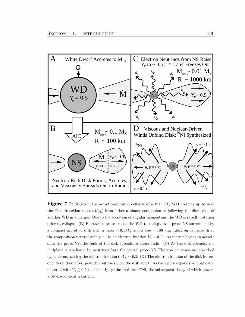
Section 7.1. Introduction 246
ννe
eν νe
56Ni
v ~ 0.1 c
Viscous and Nuclear-Driven
Ni
n, p => α
νeY ~ 0.5
Ch
Neutron-Rich Disk Forms, Accretes,and Viscously Spreads Out in Radius
Electron Neutrinos from NS Raisee
56
n, p => α
Winds Unbind Disk; Ni Synthesized56
Y to ~ 0.5 ; Y Later Freezes Oute
A C
B D
v ~ 0.1 c
ΩWhite Dwarf Accretes to M
νe
eν
e
e
M.
Y = 0.5WD
e
NS.
Y ~ 0.1
M ~ 0.01 M
v < 0 v > 0
R ~ 1000 kmDISK
M ~ 0.1 MDISK
R ~ 100 km
M
NS
NS
e
AIC
Figure 7.1: Stages in the accretion-induced collapse of a WD. (A) WD accretes up to near
the Chandrasekhar mass (MCh) from either a binary companion or following the disruption of
another WD in a merger. Due to the accretion of angular momentum, the WD is rapidly rotating
prior to collapse. (B) Electron captures cause the WD to collapse to a proto-NS surrounded by
a compact accretion disk with a mass ∼ 0.1M¯ and a size ∼ 100 km. Electron captures drive
the composition neutron-rich (i.e., to an electron fraction Ye ∼ 0.1). As matter begins to accrete
onto the proto-NS, the bulk of the disk spreads to larger radii. (C) As the disk spreads, the
midplane is irradiated by neutrinos from the central proto-NS. Electron neutrinos are absorbed
by neutrons, raising the electron fraction to Ye ∼ 0.5. (D) The electron fraction of the disk freezes
out. Soon thereafter, powerful outflows blow the disk apart. As the ejecta expands adiabatically,
material with Ye & 0.5 is efficiently synthesized into 56Ni, the subsequent decay of which powers
a SN-like optical transient.
Section 7.1. Introduction 247
similar initial properties that are formed from black hole (BH)-NS or NS-NS merg-
ers. Many of these results also apply to proto-NS accretion following AIC. Al-
though the disk is initially concentrated just outside the proto-NS surface, the
bulk of the mass of the disk must spread to larger radii as matter accretes in order
to conserve angular momentum. Early in their evolution, such “hyper-accreting”
disks are neutrino-cooled and geometrically thin, and their composition is driven
neutron-rich by an equilibrium between e−/e+ captures under degenerate condi-
tions (e.g., Pruet et al. 2003; Fig. 7.1B): the electron fraction Ye ∼ 0.1, where
Ye ≡ np/(np + nn) and np/nn are the proton/neutron number densities. As the
disk viscously spreads and its temperature decreases, however, weak interactions
eventually become slow compared to the evolution timescale of the disk and the
value of Ye freezes out.
Soon following freeze-out, neutrino cooling becomes inefficient and the disk
becomes advective and geometrically thick (Chapters 5 and 6). Since advective
disks are only marginally bound, powerful winds likely begin to unbind most of the
remaining mass of the disk (Blandford & Begelman 1999), aided by the nuclear
energy released as α−particles begin to form (Lee & Ramirez-Ruiz 2007; Chapters
5 and 6). Because ∼ 20% of the initial disk mass Md,0 still remains when the
disk becomes advective (or when α−particles form), a robust consequence of disk
formation during AIC is the ejection of up to a few times 10−2M¯. Since the ejecta
are hot and dense, heavy isotopes are synthesized as they expand away from the
midplane and cool. Because weak interactions are already slow by this point, which
heavy isotopes are produced depends on Ye in the disk at freeze-out.
In the case of BH accretion following BH-NS or NS-NS mergers, the disk
freezes out neutron-rich with an electron fraction Ye ∼ 0.2 − 0.4 (Chapters 5 and
6). A crucial difference in the case of AIC, however, is the presence of the central
proto-NS, which radiates a substantial flux of electron neutrinos as it de-leptonizes
during the first few seconds following core bounce (e.g., Burrows & Lattimer 1986).
This νe flux irradiates the disk, which acts to raise Ye via absorptions on free
neutrons (νe + n→ e− + p; Fig. 7.1C).
In §7.2 we present calculations of the evolution of the accretion disks formed
Section 7.2. AIC Accretion Disk Model 248
from AIC using time-dependent height-integrated simulations with initial condi-
tions and neutrino irradiation taken from the AIC simulations of D06. We show
that due to νe absorptions, a substantial fraction of the disk freezes out with
Ye & 0.5. As a result, late time outflows from the disk primarily synthesize 56Ni
(Fig. 7.1D). We discuss the observational signature of these Ni-rich outflows in
§7.3, and we conclude in §7.4 by evaluating the prospects for detecting AIC with
upcoming optical transient surveys and as electromagnetic counterparts to gravi-
tational wave sources.
7.2 AIC Accretion Disk Model
7.2.1 Methodology
The equations and assumptions employed here closely follow those in §6.3.1
for NS-NS or BH-NS mergers. To provide a brief summary, we evolve the surface
density Σ, temperature T , and electron fraction Ye as a function of radius r and
time t using the 2N-RK3 scheme described in Brandenburg (2001). We employ an
“α” prescription for the viscosity (Shakura & Sunyaev 1973), with the accretion
stress proportional to the gas pressure. Our calculation includes all of the relevant
neutrino cooling processes for both optically thin and optically thick disks (e.g.,
Di Matteo et al. 2002). We take the initial surface density Σ(r, t = 0) from the
Keplerian disk that forms soon after core bounce in the AIC calculations of D06.
We focus on the 1.46M¯ WD model of D06, which collapses to form a ≈ 0.1M¯
disk that extends from the NS surface at ≈ 30 km out to several NS radii (see
Fig. 5 of D06).
We evolve Ye including both local e−/e+ pair captures (e− + p → νe + n
and e+ + n → νe + p) and non-local neutrino absorptions (νe + n → e− + p and
νe + p → e+ + n) due to irradiation from the central proto-NS. We approximate
the neutrino flux from the proto-NS as arising from a “light bulb” at the origin
because the neutrino capture rates only become important relative to the pair
capture rates when the disk has spread to a radius which is much larger than that
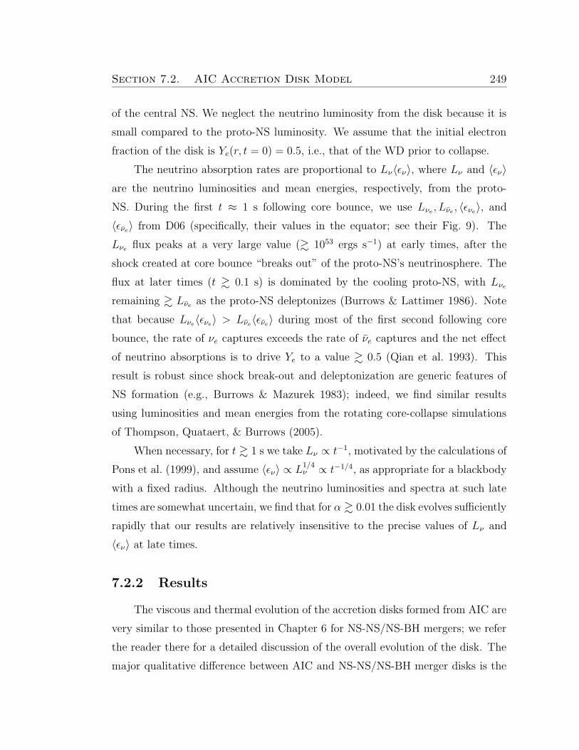
Section 7.2. AIC Accretion Disk Model 249
of the central NS. We neglect the neutrino luminosity from the disk because it is
small compared to the proto-NS luminosity. We assume that the initial electron
fraction of the disk is Ye(r, t = 0) = 0.5, i.e., that of the WD prior to collapse.
The neutrino absorption rates are proportional to Lν〈εν〉, where Lν and 〈εν〉
are the neutrino luminosities and mean energies, respectively, from the proto-
NS. During the first t ≈ 1 s following core bounce, we use Lνe , Lνe , 〈ενe〉, and
〈ενe〉 from D06 (specifically, their values in the equator; see their Fig. 9). The
Lνe flux peaks at a very large value (& 1053 ergs s−1) at early times, after the
shock created at core bounce “breaks out” of the proto-NS’s neutrinosphere. The
flux at later times (t & 0.1 s) is dominated by the cooling proto-NS, with Lνe
remaining & Lνe as the proto-NS deleptonizes (Burrows & Lattimer 1986). Note
that because Lνe〈ενe〉 > Lνe〈ενe〉 during most of the first second following core
bounce, the rate of νe captures exceeds the rate of νe captures and the net effect
of neutrino absorptions is to drive Ye to a value & 0.5 (Qian et al. 1993). This
result is robust since shock break-out and deleptonization are generic features of
NS formation (e.g., Burrows & Mazurek 1983); indeed, we find similar results
using luminosities and mean energies from the rotating core-collapse simulations
of Thompson, Quataert, & Burrows (2005).
When necessary, for t & 1 s we take Lν ∝ t−1, motivated by the calculations of
Pons et al. (1999), and assume 〈εν〉 ∝ L1/4ν ∝ t−1/4, as appropriate for a blackbody
with a fixed radius. Although the neutrino luminosities and spectra at such late
times are somewhat uncertain, we find that for α & 0.01 the disk evolves sufficiently
rapidly that our results are relatively insensitive to the precise values of Lν and
〈εν〉 at late times.
7.2.2 Results
The viscous and thermal evolution of the accretion disks formed from AIC are
very similar to those presented in Chapter 6 for NS-NS/NS-BH mergers; we refer
the reader there for a detailed discussion of the overall evolution of the disk. The
major qualitative difference between AIC and NS-NS/NS-BH merger disks is the
Section 7.2. AIC Accretion Disk Model 250
0.001
0.010
M(Y
e) (
MO • b
in-1)
0.35 0.40 0.45 0.50 0.55 0.60 0.65Ye
0.001
0.010
M(Y
e) (
MO • b
in-1)
90% Advective
90% α-Particles
α = 0.3, t = 0.2 s α = 0.03, t = 7 s
α = 0.3, t = 0.6 s α = 0.03, t = 7 s
Figure 7.2: Amount of mass with a given electron fractionM(Ye) in the accretion disk formed
from AIC for a model with an initial mass distribution and neutrino irradiation from the 1.46M¯
WD AIC simulation of D06. The top and bottom panels correspond to times when 90% of the
mass of the disk is advective and has formed α−particles, respectively. The solid and dashed
lines show results for α = 0.3 and α = 0.03, respectively.
Section 7.2. AIC Accretion Disk Model 251
evolution of the electron fraction, so we focus on our results for Ye below.
Figure 7.2 shows histograms of mass as a function of electron fraction M(Ye)
for our fiducial model that employs an initial density profile and neutrino irra-
diation from the 1.46M¯ WD model of D06. The solid and dashed lines show
calculations performed with viscosity α = 0.3 and α = 0.03, respectively. The
top panel shows M(Ye) when 90% of the mass of the disk has become advective,
which corresponds to a time t = 0.2(7) s for α = 0.3(0.03). Annuli in the disk
are considered advective once the neutrino cooling rate becomes . 1/2 of the
viscous heating rate. The bottom panel shows M(Ye) when 90% of the mass of
the disk has fused into α−particles, which corresponds to a time t = (0.6)7 s for
α = 0.3(0.03). Although powerful outflows likely begin when the disk becomes
advective (Blandford & Begelman 1999), thermonuclear disruption of the disk is
assured once α−particles form. This occurs because (1) the nuclear reactions that
create (and destroy) deuterium (the building blocks of α−particles) are still very
fast compared to the evolution timescale of the disk (i.e., the disk is still in nu-
clear statistical equilibrium [NSE]) when the temperature drops sufficiently that
the NSE α−particle mass fraction becomes ∼ unity (e.g., Chen & Beloborodov
2007, eq. [13]); and (2) the energy released by forming α−particles (∼ 7 MeV per
nucleon) exceeds the gravitational binding energy of the disk (see Chapters 5 and
6). Thus, the distributions in Figure 7.2 roughly bracket the distribution of Ye in
the outflows that carry away the remaining mass in the disk at late times.
Figure 7.2 shows that ≈ 0.02 − 0.03M¯ (or ≈ 20 − 30% of the initial disk
mass) remains when the disk is largely advective. A comparable amount of mass
remains when the disk forms α−particles because this occurs at approximately the
same time (Chapters 5 and 6; Beloborodov 2008). Although the bulk of the disk
is initially driven neutron-rich by degenerate electron captures, Figure 7.2 shows
that a large portion of the mass remaining at late times has Ye & 0.5. As discussed
in §7.1.1, the disk composition is driven proton-rich by the powerful νe flux from
the central proto-NS.
We have performed similar calculations for other disk parameters in order
to study the sensitivity of our results to the initial properties of the disk (see
Section 7.3. Optical Transients from AIC 252
Table 7.1). For example, the disks found by D06,07 are fairly massive, but a less
massive disk would result from a slower rotating WD. Thus, we have also performed
calculations using the same initial density profile from D06, but normalizing the
total initial disk mass toMd,0 = 0.01M¯ instead of 0.1M¯. We have also calculated
models with Σ(r, t = 0), Lν(t) and 〈εν〉(t) taken from the rapidly rotating, 1.92M¯
WD model of D06, which formed a more massive initial disk (Md,0 ≈ 0.5M¯). In
the highMd,0 case we find that a significant fraction of the disk has exactly Ye = 0.5
at freeze-out. This occurs because in this model α−particle formation precedes
weak freeze-out; thus, any excess free neutrons or protons are almost immediately
captured into α−particles (which have Ye = 0.5) following a neutrino absorption
(the “alpha-effect” of Fuller & Meyer 1995). We note, however, that torques within
an accreting WD will probably prevent it from having sufficient differential rotation
to support the large WD masses needed to form such a massive disk (Piro 2008);
these models may still be achievable through the merger of two massive WDs.
In Table 7.1 we summarize our results for the total mass (Madv) and the total
mass with 0.485 . Ye . 0.6 (MNi) when the disk has become 90% advective. The
latter is labeled MNi because a significant fraction of the mass ejected with Ye in
this range produces 56Ni (see §7.3). In all cases, we find that a significant fraction
(& 50%) of the mass remaining at late times has Ye & 0.5. Thus, under a variety
of conditions, AIC leads to ∼ 10% of the initial disk being ejected as moderately
proton-rich material.
7.3 Optical Transients from AIC
In some ways, AIC can be considered a “failed” Type Ia SN because it does
not produce ∼ 1M¯ of shock-heated ejecta. Indeed, the total 56Ni mass ejected
from the proto-NS is . 10−3M¯ (e.g., Woosley & Baron 1992; D06,07; Chapter
4), rendering isolated NS birth practically invisible. In the presence of rotation,
however, this failure is not complete. In §7.2 we showed that if an accretion
disk forms around the proto-NS during collapse, a natural consequence of the
subsequent evolution of the disk is that up to ∼ 10−2M¯ of material with Ye & 0.5
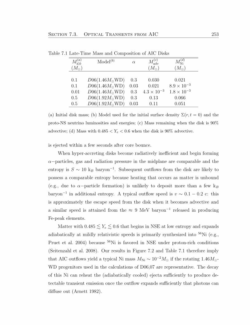
Section 7.3. Optical Transients from AIC 253
Table 7.1 Late-Time Mass and Composition of AIC Disks
M(a)d,0 Model(b) α M
(c)adv M
(d)Ni
(M¯) (M¯) (M¯)
0.1 D06(1.46M¯WD) 0.3 0.030 0.0210.1 D06(1.46M¯WD) 0.03 0.021 8.9× 10⁻³
0.01 D06(1.46M¯WD) 0.3 4.3× 10⁻³ 1.8× 10⁻³
0.5 D06(1.92M¯WD) 0.3 0.13 0.0660.5 D06(1.92M¯WD) 0.03 0.11 0.051
(a) Initial disk mass; (b) Model used for the initial surface density Σ(r, t = 0) and the
proto-NS neutrino luminosities and energies; (c) Mass remaining when the disk is 90%
advective; (d) Mass with 0.485 < Ye < 0.6 when the disk is 90% advective.
is ejected within a few seconds after core bounce.
When hyper-accreting disks become radiatively inefficient and begin forming
α−particles, gas and radiation pressure in the midplane are comparable and the
entropy is S ∼ 10 kB baryon−1. Subsequent outflows from the disk are likely to
possess a comparable entropy because heating that occurs as matter is unbound
(e.g., due to α−particle formation) is unlikely to deposit more than a few kB
baryon−1 in additional entropy. A typical outflow speed is v ∼ 0.1 − 0.2 c: this
is approximately the escape speed from the disk when it becomes advective and
a similar speed is attained from the ≈ 9 MeV baryon−1 released in producing
Fe-peak elements.
Matter with 0.485 . Ye . 0.6 that begins in NSE at low entropy and expands
adiabatically at mildly relativistic speeds is primarily synthesized into 56Ni (e.g.,
Pruet et al. 2004) because 56Ni is favored in NSE under proton-rich conditions
(Seitenzahl et al. 2008). Our results in Figure 7.2 and Table 7.1 therefore imply
that AIC outflows yield a typical Ni mass MNi ∼ 10−2M¯ if the rotating 1.46M¯-
WD progenitors used in the calculations of D06,07 are representative. The decay
of this Ni can reheat the (adiabatically cooled) ejecta sufficiently to produce de-
tectable transient emission once the outflow expands sufficiently that photons can
diffuse out (Arnett 1982).
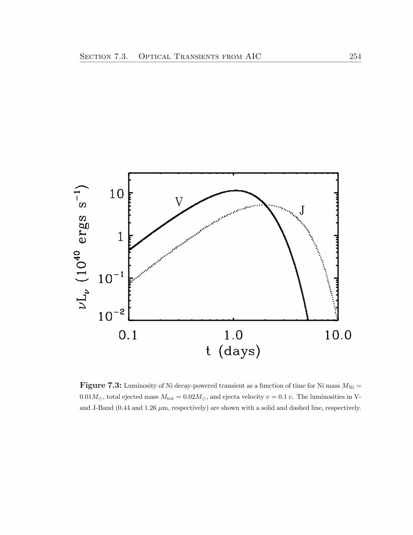
Section 7.3. Optical Transients from AIC 254
Figure 7.3: Luminosity of Ni decay-powered transient as a function of time for Ni massMNi =
0.01M¯, total ejected massMtot = 0.02M¯, and ejecta velocity v = 0.1 c. The luminosities in V-
and J-Band (0.44 and 1.26 µm, respectively) are shown with a solid and dashed line, respectively.
Section 7.4. Detection Prospects 255
We explore this possibility by calculating the light curves of ejecta heated by
Ni decay using the method of Kulkarni (2005) and Chapter 5. Figure 7.3 shows
the V and J-band luminosities as a function of time since collapse for an outflow
with Ni mass MNi = 10−2M¯ and total ejecta mass Mtot = 2× 10⁻²M¯ expanding
at v = 0.1 c. The total luminosity peaks in the visual (V-band) on a ∼ 1 day
timescale, with νLν ∼ 1041 ergs s−1. The J-band light curve peaks somewhat later
than V-band because the temperature at the photosphere decreases as the material
expands. We discuss the likelihood of detecting such a transient with blind surveys
in §7.4.
Although 56Ni is likely to be the dominant isotope synthesized, other isotopes
will also be produced in smaller abundances. For instance, under the conditions of
interest ∼ 10% of the ejected mass may remain in the form of α−particles (Woosley
& Hoffman 1992). Furthermore, our low-α calculations in Figure 7.2 indicate that
some fraction of the material ejected may have Ye . 0.485 (Fig. 7.2). In this
case, freeze-out from NSE produces both stable (e.g., 58,60,62,64Ni, 54,56,58Fe) and
radioactive (e.g., 66,68,70Ni, 60,62,66Zn) Fe-group elements instead of 56Ni (Woosley &
Hoffman 1992). Although this material will contribute to the opacity of the outflow
(Mtot above), its additional contribution to the radioactive heating is unlikely to
substantially alter the purely Ni-powered light curves in Figure 7.3.
7.4 Detection Prospects
Because AIC has never been observationally identified, its rate is uncertain.
Binary population synthesis models predict galactic rates in the range RAIC ∼
10−6−10−4 yr−1 (e.g., Yungelson & Livio 1998). The amount of highly neutron-rich
material ejected per AIC can also be used to constrain the AIC rate (Hartmann
et al. 1985; Fryer et al. 1999): if the ∼ 3 × 10⁻³M¯ of ejected material with
Ye . 0.4 in the calculations of D06 is representative, RAIC must be . 10−4 yr−1
so as not to over-produce the abundances of neutron-rich isotopes in our solar
system. If the proto-NS forms with a strong large-scale magnetic field ∼ 1015 G,
then a much larger quantity ∼ 0.1M¯ of neutron-rich material is ejected by the
Section 7.4. Detection Prospects 256
proto-NS’s magneto-centrifugally driven wind (D07; Chapter 4) and the AIC rate
is constrained to be even lower.
Assuming that the AIC rate is proportional to the blue stellar luminosity
(Phinney 1991), a Galactic rate of RAIC ≡ 10−4R−4 yr−1 corresponds to a vol-
umetric rate of 10−6R−4 Mpc−3 yr−1. For the 1.46M¯-WD model of D06, we
predict that AIC produces an optical transient with a peak luminosity ∼ 1041 ergs
s−1 (Fig. 7.3). This corresponds to a maximum detection distance of 650(410)[100]
Mpc for a limiting magnitude of 25(24)[21]. Thus, the Pan-STARRs Medium Deep
Survey (MDS; Kaiser et al. 2002), which covers ∼ 84 deg2 in g and r down to AB
magnitude 25, will detect ∼ 2.4R−4 yr−1. The Palomar Transient Factory (PTF;
Rau et al. 2008), which surveys ∼ 8000 deg2 to a limiting AB magnitude of 21,
will detect 0.9R−4 yr−1. Thus, if RAIC ∼ 10−4 yr−1, MDS and PTF should detect
a few AIC events per year. Prospects for detection are much better with the Large
Synoptic Survey Telescope (LSST; LSST collaboration 2007), which will image the
entire sky down to a limiting magnitude ∼ 24.5 every 3–4 nights and should detect
AIC events at a rate ∼ 800R−4 yr−1. The short, few-day timescale of the transient
requires observations with high cadence. Shallow, wider-area surveys such as PTF
may be preferable because separating the transient from its host galaxy’s light may
be difficult for high redshift events.
The detectability of an optical transient is sensitive to whether there is suf-
ficient mass in a remnant disk, which in turn depends on the angular momentum
distribution of the WD progenitor. The very massive AIC progenitor from D06
(1.92M¯) is consistent with the large shear found by Yoon & Langer (2004, 2005),
who studied angular momentum transport by Kelvin-Helmholtz instabilities dur-
ing accretion. Piro (2008) argued, however, that large magnetic stresses impose
nearly solid body rotation, which prevents the WD from reach a mass much over
the (non-rotating) Chandrasekhar limit (this may also be the case for purely hy-
drodynamic instabilities; see Saio & Nomoto 2004). More work is needed to un-
derstand the possible progenitors of AIC, and the resulting implications for the
accretion disk formed during collapse, taking into account the effects of magnetic
stresses and compositional gradients on the redistribution of angular momentum
Section 7.4. Detection Prospects 257
during accretion.
Other thermal transients are predicted to occur in nature on ∼ day timescales,
such as “.Ia” SNe due to unstable thermonuclear He flashes from WD binaries
(Bildsten et al. 2007). Although such events may originate from a similar stellar
population and could be confused with AIC, a defining characteristic of AIC out-
flows is that most of the ejected material is processed through low entropy NSE.
As a result, we expect few intermediate-mass elements to be produced (such as O,
Ca, and Mg), although small amounts of He may be present. Thus, the Ni-rich
explosions produced by AIC should be spectroscopically distinct from other types
of SN identified to date.
The timescale, velocity, and composition of the AIC transient can be modified
if significant amounts of WD material remain at large radii following AIC, either
because the WD is still collapsing at late times or because some matter remains
centrifugally supported in a remnant disk created by a super-MCh WD-WD merger
(e.g., Yoon et al. 2007). In the later case, depending on the mass and composition
of the WD binary, up to ∼ 0.1M¯ in C, O, Ne, or He could remain at a radius
R ∼ 109 cm. Once the Ni wind (with energy ∼ 1050 ergs) impacts this remnant
material, it will (1) shock heat the material to a few times 109 K, which may
synthesize intermediate mass elements (Woosley & Weaver 2002), but will not
disassociate the Ni and will likely leave some unburned WD material; (2) slow the
ejecta, by conservation of momentum, from v ∼ 0.1 c to a few thousand km s−1. A
combination of slower ejecta and higher opacity would also lengthen the duration
of the light curve by a factor of ∼ 10 from that shown in Figure 7.3, making such
an event easier to detect. Indeed, such an “enshrouded AIC” model represents
a possible explanation for sub-luminous, sub-Chandrasekhar Type I SNe, such as
2008ha, which rose to its peak brightness in only ∼ 10 days, possessed low line
velocities (∼ 2000 km s−1), and was inferred to have MNi ≈ 3 × 10⁻³M¯ and
Mtot ∼ 0.15M¯ (Foley et al. 2009). We plan to study this possibility further, as
well as explore the interaction between the disk wind and the outoing SN shock,
in future work.
AIC may also be detectable with upcoming km-scale gravitational wave (GW)
Section 7.4. Detection Prospects 258
detectors such as Advanced LIGO (Abramovici et al. 1992). If the collapse remains
axisymmetric, the detection of AIC in GWs appears unlikely except within the
Milky Way (D06,07; Dimmelmeier et al. 2008). However, if the progenitor WD
is very rapidly rotating (as may result following a WD-WD merger), the ratio of
rotational to gravitational energy of the proto-NS upon collapse may be sufficiently
large for the growth of nonaxisymmetric instabilities, which would greatly increase
the GW signal and detection prospects (Fryer et al. 2002; Ott 2008). Indeed, D06
find that their their 1.92 M¯-WD model rotates sufficiently rapidly to trigger a
dynamically unstable spiral mode upon collapse (Ott et al. 2005). We note that
our calculations predict that large Ni yields will accompany the massive disks that
form from such rapidly rotating progenitors (e.g., we findMNi ≈ 0.07M¯ for D06’s
1.92M¯ model; see Table 7.1). Thus, events accompanied by GW emission that is
detectable to extragalactic distances will likely produce a somewhat brighter SN
transient than our fiducial example in Figure 7.3. More generally, the brightness
of the optical emission from AIC directly traces the importance of rotation during
the collapse.
Acknowledgements
We thank Luc Dessart for providing his AIC calculations. We also thank Todd
Thompson for helpful conversations and for providing the neutrino luminosity and
spectral evolution from his rotating core-collapse supernova calculations. A. L. P. is
supported by the Theoretical Astrophysics Center at UC Berkeley. B. D. M and
E. Q. were supported in part by the David and Lucile Packard Foundation, NASA
grant NNG05GO22H, and the NSF-DOE Grant PHY-0812811.
259
Bibliography
IceCube Collaboration: R. Abbasi 2009, arXiv:0902.0131
Abdo, A. A., et al. 2009, “Fermi Observations of High-Energy Gamma-Ray Emis-
sion from GRB 080916C” , accepted to Science, Feb. 11 2009
Abramovici, A., et al. 1992, Science, 256, 325
Aharonian, F., et al. 2007, ApJ, 664, L71
Akiyama, S., Wheeler, J. C., Meier, D. L., & Lichtenstadt, I. 2003, ApJ, 584, 954
Arnett, W. D. 1982, ApJ, 253, 785
Arons, J., & Scharlemann, E. T. 1979, ApJ, 231, 854
Atteia, J.-L., et al. 1987, ApJS, 64, 305
Bahcall, J. N., & Meszaros, P. 2000, Physical Review Letters, 85, 1362
Bailyn, C. D., & Grindlay, J. E. 1990, ApJ, 353, 159
Balbus, S. A., & Hawley, J. F. 1998, Reviews of Modern Physics, 70, 1
Barkana, R., & Loeb, A. 2001, Phys. Rep., 349, 125
Barthelmy, S. D., et al. 2005, Nature, 438, 994
Barthelmy, S., et al. 2005, GRB Coordinates Network, 3385, 1
Barzilay, Y., & Levinson, A. 2008, New Astronomy, 13, 386
BIBLIOGRAPHY 260
Baumgarte, T. W., Shapiro, S. L., & Shibata, M. 2000, ApJ, 528, L29
Begelman, M. C., & Li, Z.-Y. 1992, ApJ, 397, 187
Belcher, J. W., & MacGregor, K. B. 1976, ApJ, 210, 498
Belczynski, K., Perna, R., Bulik, T., Kalogera, V., Ivanova, N., & Lamb, D. Q.
2006, ApJ, 648, 1110
Bell, A. R. 2004, MNRAS, 353, 550
Beloborodov, A. M. 2003a, ApJ, 588, 931 (B03a)
Beloborodov, A. M. 2003b, ApJ, 585, L19
Beloborodov, A. M. 2008, American Institute of Physics Conference Series, 1054,
51
Berger, E., et al. 2003, Nature, 426, 154
Berger, E., Kulkarni, S. R., & Frail, D. A. 2003, ApJ, 590, 379
Berger, E., et al. 2005, Nature, 438, 988
Bethe, H. A., & Brown, G. E. 1998, ApJ, 506, 780
Bethe, H. A., Brown, G. E., & Lee, C.-H. 2007, Physics Reports, 442, 5
Bethe, H. A., & Wilson, J. R. 1985, ApJ, 295, 14
Bildsten, L. & Cutler, C. 1992, ApJ, 400, 175
Bildsten, L., Shen, K. J., Weinberg, N. N., & Nelemans, G. 2007, ApJ, 662, L95
Binney, J., & Tremaine, S. 1994, “Galactic Dynamics” (Second Edition), Princeton
University Press
Blackman, E. G., & Yi, I. 1998, ApJ, 498, L31
BIBLIOGRAPHY 261
Blaes, O. M., Davis, S. W., Hirose, S., Krolik, J. H., & Stone, J. M. 2006b, ApJ,
645, 1402
Blaes, O. 2007, ArXiv Astrophysics e-prints, arXiv:astro-ph/0703589
Blandford, R. D. 2002, Lighthouses of the Universe: The Most Luminous Celestial
Objects and Their Use for Cosmology, 381
Blandford, R. D., & Begelman, M. C. 1999, MNRAS, 303, L1
Blandford, R. D., & McKee, C. F. 1976, Physics of Fluids, 19, 1130
Blandford, R. D., & Payne, D. G. 1982, MNRAS, 199, 883
Blinnikov, S. I., Novikov, I. D., Perevodchikova, T. V., & Polnarev, A. G. 1984,
Soviet Astronomy Letters, 10, 177
Blondin, J. M., Mezzacappa, A., & DeMarino, C. 2003, ApJ, 584, 971
Bloom, J. S., et al. 1999, ApJ, 518, L1
Bloom, J. S., Frail, D. A., & Kulkarni, S. R. 2003, ApJ, 594, 674
Bloom, J. S., Butler, N. R., & Perley, D. A. 2008, American Institute of Physics
Conference Series, 1000, 11
Bloom, J. B., et al. 2005, Bulletin of the American Astronomical Society, 37, 793
Bloom, J. S., et al. 2006, ApJ, 638, 354
Bloom, J. S., & Prochaska, J. X. 2006, Gamma-Ray Bursts in the Swift Era, 836,
473
Brandenburg, A. 2003, in Advances in Nonlinear Dynamos: The Fluid Mechanics
of Astrophysics & Geophysics, Vol 9, ed. A. Ferriz-Mas & M. Nunez (London,
New York: Taylor & Francis), 269
Bruenn, S. W., De Nisco, K. R., & Mezzacappa, A. 2001, ApJ, 560, 326
BIBLIOGRAPHY 262
Bucciantini, N., Thompson, T. A., Arons, J., Quataert, E., & Del Zanna, L. 2006,
MNRAS, 368, 1717
Bucciantini, N., Quataert, E., Arons, J., Metzger, B. D., & Thompson, T. A. 2007,
MNRAS, 380, 1541
Bucciantini, N., Quataert, E., Arons, J., Metzger, B. D., & Thompson, T. A. 2008,
MNRAS, 383, L25
Bucciantini, N., Quataert, E., Metzger, B. D., Thompson, T. A., Arons, J., & Del
Zanna, L. 2009, arXiv:0901.3801
Bulik, T., Sikora, M., & Moderski, R. 2002, ArXiv Astrophysics e-prints,
arXiv:astro-ph/0209339
Buras, R., Rampp, M., Janka, H.-T., & Kifonidis, K. 2003, Physical Review Let-
ters, 90, 241101
Buras, R., Rampp, M., Janka, H.-T., & Kifonidis, K. 2006, A&A, 447, 1049
Burrows, A., Hayes, J., & Fryxell, B.A. 1995, ApJ, 450, 830
Burrows, A., & Lattimer, J. M. 1986, ApJ, 307, 178
Burrows, A., & Mazurek, T. L. 1983, Nature, 301, 315
Burrows, A., Livne, E., Dessart, L., Ott, C. D., & Murphy, J. 2006, ApJ, 640, 878
Burrows, A., Livne, E., Dessart, L., Ott, C. D., & Murphy, J. 2006, New Astronomy
Review, 50, 487
Burrows, A., & Mazurek, T. J. 1982, ApJ, 259, 330
Burrows, D. N., et al. 2005, Science, 309, 1833
Butler, N. R., & Kocevski, D. 2007, ApJ, 663, 407
Campana, S., et al. 2006, A&A, 454, 113
BIBLIOGRAPHY 263
Canal, R., Isern, J., & Labay, J. 1990, ARAA, 28, 183
Chang, P., Spitkovsky, A., & Arons, J. 2008, ApJ, 674, 378
Cardall, C. Y., & Fuller, G. M. 1997, ApJ, 486, L111
Cavallo, G., & Rees, M. J. 1978, MNRAS, 183, 359
Chen, W.-X., & Beloborodov, A. M. 2007, ApJ, 657, 383
Chevalier, R. A. 1989, ApJ, 346, 847
Colgate, S. A., Petschek, A. G., & Kriese, J. T. 1980, ApJ, 237, L81
Contopoulos, J. 1994, ApJ, 432, 508
Contopoulos, I., Kazanas, D., & Fendt, C. 1999, ApJ, 511, 351
Cook, G. B., Shapiro, S. L., & Teukolsky, S. A. 1994, ApJ, 424, 823
Costa, E., et al. 1997, Nature, 387, 783
Couch, S. M., Milosavljevic, M., & Nakar, E. 2008, ApJ, 688, 462
Cowan, J. J., et al. 2005, ApJ, 627, 238
Cranmer, S. R., & van Ballegooijen, A. A. 2005, ApJS, 156, 265
Dai, Z. G., et al. 2006, Science, 311, 1127
Daigne, F., & Mochkovitch, R. 2002, A&A, 388, 189 (DM02)
Delano, M. D., & Cameron, A. G. W. 1971, Astrophys. Space Sci. , 10, 203
Della Valle, M., et al. 2006, ArXiv Astrophysics e-prints, arXiv:astro-ph/0608322
Del Zanna, L., Volpi, D., Amato, E., & Bucciantini, N. 2006, A&A, 453, 621
Derishev, E. V., Kocharovsky, V. V., & Kocharovsky, V. V. 1999, ApJ, 521, 640
Dermer, C. D., & Atoyan, A. 2006, New Journal of Physics, 8, 122
BIBLIOGRAPHY 264
Dessart, L., Burrows, A., Ott, C. D., Livne, E., Yoon, S.-Y., & Langer, N. 2006,
ApJ, 644, 1063
Dessart, L., et al. 2007, ApJ, 669, 585 (D07)
Dessart, L., Burrows, A., Livne, E., & Ott, C. D. 2008, ApJ, 673, L43
Di Matteo, T., Perna, R., & Narayan, R. 2002, ApJ, 579, 706
Dimmelmeier, H., Ott, C. D., Marek, A., & Janka, H.-T. 2008, Phys. Rev. D, 78,
064056
Drenkhahn, G., & Spruit, H. C. 2002, A&A, 391, 1141
Duan, H., & Qian, Y.-Z. 2004, Phys. Rev. D, 69, 123004
Duez, M. D., Liu, Y. T., Shapiro, S. L., Shibata, M., & Stephens, B. C. 2006,
Phys. Rev. D, 73, 104015
Duez, M. D., Liu, Y. T., Shapiro, S. L., & Stephens, B. C. 2004, Phys. Rev. D,
69, 104030
Duncan, R. C., Shapiro, S. L., & Wasserman, I. 1986, ApJ, 309, 141
Duncan, R. C., & Thompson, C. 1992, ApJ, 392, L9
Eichler, D., & Levinson, A. 1999, ApJ, 521, L117
Eichler, D., Livio, M., Piran, T., & Schramm, D. N. 1989, Nature, 340, 126
Faber, J. A., et al. 2006a, Phys. Rev. D, 73, 4012
Faber, J. A., et al. 2006b, ApJ, 641, L93
Falcone, A. D., et al. 2007, ApJ, 671, 1921
Fan, Y. Z., & Wei, D. M. 2004, ApJ, 615, L69
Fan, Y. Z., Zhang, B., & Wei, D. M. 2005, ApJ, 628, L25
BIBLIOGRAPHY 265
Fender, R., et al. 2004, Nature, 427, 222
Ferrero, P., et al. 2007, AJ, 134, 2118
Fishbone, L. G. 1973, ApJ, 185, 43
Fishman, G. J., & Meegan, C. A. 1995, ARA&A, 33, 415
Foley, R. J., et al. 2009, arXiv:0902.2794
Fox, D. B., et al. 2005, Nature, 437, 845
Frail, D. A., Kulkarni, S. R., Nicastro, L., Feroci, M., & Taylor, G. B. 1997, Nature,
389, 261
Frail, D. A., et al. 2001, ApJ, 562, L55
Frank, J., King, A. R., & Raine, D. J. 2002, Accretion Power in Astrophysics (3rd
ed.; Cambridge: Cambridge Univ. Press)
Freiburghaus, C., Rosswog, S., & Thielemann, F.-K. 1999, ApJ, 525, L121
Fruchter, A. S., et al. 2006, Nature, 441, 463
Fryer, C., Benz, W., Herant, M., & Colgate, S. A. 1999, ApJ, 516, 892
Fryer, C. L., & Heger, A. 2000, ApJ, 541, 1033
Fryer, C. L., Holz, D. E., & Hughes, S. A. 2002, ApJ, 565, 430
Fryer, C. L., Woosley, S. E., Herant, M., & Davies, M. B. 1999b, ApJ, 520, 650
Fuller, G. M., & Meyer, B. S. 1995, ApJ, 453, 792
Fuller, G. M., & Qian, Y.-Z. 1996, Nucl. Phys. A, 606, 167
Fynbo, J.P.U., et al. 2006, preprint (astro-ph/0608313)
Galama, T. J., et al. 1998, Nature, 395, 670
BIBLIOGRAPHY 266
Gal-Yam, A., et al. 2006, Nature, 444, 1053
Gao, W.-H., & Fan, Y.-Z. 2006, ChJAA, 6, 513
Gehrels, N. et al, 2005, Nature, 437, 851
Gehrels, N., et al. 2006, Nature, 444, 1044
Genet, F., Daigne, F., & Mochkovitch, R. 2007, MNRAS, 381, 732
Ghirlanda, G., Nava, L., Ghisellini, G., Celotti, A., & Firmani, C. 2009,
arXiv:0902.0983
Ghosh, P., & Lamb, F. K. 1978, ApJ, 223, L83
Giannios, D., & Spruit, H. C. 2005, A&A, 430, 1
Giannios, D. 2007, ArXiv e-prints, 704, arXiv:0704.1659
Goodman, J. 1986, ApJ, 308, L47
Goodman, J., & MacFadyen, A. I. 2007, arXiv:0706.1818
Granot, J., & Kumar, P. 2006, MNRAS, 366, L13
Grindlay, J. E. 1987, The Origin and Evolution of Neutron Stars, 125, 173
Grindlay, J. E., & Bailyn, C. D. 1988, Nature, 336, 48
Grupe, D., Burrows, D. N., Patel, S. K., Kouveliotou, C., Zhang, B., Meszaros,
P., Wijers, R. A. M., & Gehrels, N. 2006, ApJ, 653, 462
Gruzinov, A., 2005, Physical Review Letters, 94
Guetta, D., Piran, T., & Waxman, E. 2005, ApJ, 619, 412
Gutierrez, J., Canal, R., & Garcıa-Berro, E. 2005, A&A, 435, 231
Haensel, P., & Zdunik, J. L. 1990a, A&A, 227, 431
BIBLIOGRAPHY 267
Haensel, P., & Zdunik, J. L. 1990b, A&A, 229, 117
Hartmann, D., Woosley, S. E., & El Eid, M. F. 1985, ApJ, 297,
Hawley, J. F., & Balbus, S. A. 2002, ApJ, 573, 738
Hawley, J. F., Balbus, S. A., & Stone, J. M. 2001, ApJ, 554, L49
Hawley, J. F., Gammie, C. F., & Balbus, S. A. 1995, ApJ, 440, 742
Herant, M., Benz, W., Hix, W. R., Fryer, C. L., & Colgate, S. A. 1994, ApJ, 435,
339
Hillebrandt, W., Wolff, R. G., & Nomoto, K. 1984, A&A, 133, 175
Hirose, S., Krolik, J. H., & Stone, J. M. 2006, ApJ, 640, 901
Hjorth, J., et al. 2003, Nature, 423, 847
Hjorth, J., et al. 2005, ApJ, 630, L117
Hoffman, R. D., Woosley, S. E., & Qian, Y.-Z. 1997, ApJ, 482, 951
Hughes, S. A. 2003, Annals of Physics, 303, 142
Hughes, S. A., & Holz, D. E. 2003, Classical and Quantum Gravity, 20, 65
Hurley, K., et al. 1994, Nature, 372, 652
Iwamoto, K., et al. 1998, Nature, 395, 672
Janiuk, A., Perna, R., DiMatteo, T., & Czerny, B. 2004, MNRAS, 355, 950
Janka, H.-T., Eberl, T., Ruffert, M., & Fryer, C. L. 1999, ApJ, 527, L39
Janka, H.-T., & Mueller, E. 1995, ApJ, 448, L109
Kaiser, N. et al. 2002 Proc. of the SPIE, 4836, 154
Kalogera, V., et al. 2004, ApJ, 601, L179
BIBLIOGRAPHY 268
Kaspi, V. M., & Helfand, D. J. 2002, Neutron Stars in Supernova Remnants, 271,
3
Katz, J. I. 1997, ApJ, 490, 633
Kennel, C. F., & Coroniti, F. V. 1984, ApJ, 283, 694
Kim, C., Kalogera, V., & Lorimer, D. R. 2006, ArXiv Astrophysics e-prints,
arXiv:astro-ph/0608280
King, A. R., Pringle, J. E., & Wickramasinghe, D. T. 2001, MNRAS, 320, L45
King, A. R., et al. 2005, ApJ, 630, L113
King, A. R., Pringle, J. E., & Livio, M. 2007, MNRAS, 376, 1740
Klebesadel, R. W., Strong, I. B., & Olson, R. A. 1973, ApJ, 182, L85
Kluzniak, W. & Lee, W. H. 1998, ApJ, 494, L53
Kluzniak, W., & Ruderman, M. 1998, ApJ, 505, L113
Kochanek, C. S., & Piran, T. 1993, ApJ, 417, L17
Kohri, K. & Mineshige, S. 2002,ApJ, 577, 311
Komissarov, S. S., & Barkov, M. V. 2007, MNRAS, 382, 1029
Kopal, Z. 1959, Close Binary Systems (London: Chapman & Hall)
Kouveliotou, C., Meegan, C. A., Fishman, G. J., Bhat, N. P., Briggs, M. S.,
Koshut, T. M., Paciesas, W. S., & Pendleton, G. N. 1993, ApJ, 413, L101
Kouveliotou, C., et al. 1994, Nature, 368, 125
Kouveliotou, C., et al. 1998, Nature, 393, 235
Krolik, J. H., Hirose, S., & Blaes, O. 2007, ApJ, 664, 1045
Kulkarni, S. R. 2005, ArXiv Astrophysics e-prints, arXiv:astro-ph/0510256
BIBLIOGRAPHY 269
Kulkarni, S. R., et al. 1999, Nature, 398, 389
Kumar, P., & Narayan, R. 2008, arXiv:0812.0021
Kumar, P., Narayan, R., & Johnson, J. L. 2008, MNRAS, 388, 1729
Kumar, P., & McMahon, E. 2008, MNRAS, 384, 33
LSST Collaboration, LSST Science Case.
http://www.lsst.org/Science/lsst baseline.shtml
Langer, N., Cantiello, M., Yoon, S.-C., Hunter, I., Brott, I., Lennon, D., de Mink,
S., & Verheijdt, M. 2008, IAU Symposium, 250, 167
Lai, D., Rasio, F. A., & Shapiro, S. L. 1994, ApJ, 423, 344
Lai, D., & Qian, Y.-Z. 1998, ApJ, 505, 844
La Parola, V., et al. 2006, A&A, 454, 753
Lamers, H., & Cassinelli, J. P. 1999, Introduction to Stellar Winds (Cambridge:
Cambridge University Press)
Lattimer, J. M., & Schramm, D. N. 1974, ApJ, 192, L145
Lattimer, J. M., & Schramm, D. N. 1976, ApJ, 210, 549
Lazzati, D., Ramirez-Ruiz, E., & Ghisellini, G. 2001, A&A, 379, L39
Lazzati, D., & Perna, R. 2007, MNRAS, 375, L46
Lazzati, D., Perna, R., & Begelman, M. C. 2008, MNRAS, 388, L15
Lee, W. H. & Kluzniak, W. 1995, Acta Astron., 45, 705
Lee, W. H. & Kluzniak, W. 1998, ApJ, 526, 178
Lee, W. H. & Kluzniak, W. 1999, MNRAS, 308, 780
Lee, W. H., Ramirez-Ruiz, E., & Page, D. 2004, ApJ, 608, L5
BIBLIOGRAPHY 270
Lee, W. H., Ramirez-Ruiz, E., & Page, D. 2005, ApJ, 632, 421 (L05)
Lee, W. & Ramirez-Ruiz, E. 2007, New J. Phys., 9, 17
Lemoine, M. 2002, A&A, 390, L31
Levan, A. J., et al. 2006, MNRAS, 368, L1
Levinson, A. 2006, ApJ, 648, 510
Levinson, A., & Eichler, D. 1993, ApJ, 418, 386
Levinson, A., & Eichler, D. 2003, ApJ, 594, L19 (LE03)
Li, L.-X., & Paczynski, B. 1998, ApJ, 507, L59
Li, Z.-Y., Chiueh, T., & Begelman, M. C. 1992, ApJ, 394, 459
Lightman, A. P., & Eardley, D. M. 1974, ApJ, 187, L1
Lithwick, Y., & Sari, R. 2001, ApJ, 555, 540
Lyne, A. G., et al. 1998, MNRAS, 295, 743
Lyutikov, M., & Blackman, E. G. 2001, MNRAS, 321, 177
Lyutikov, M., & Blandford, R. 2003, arXiv:astro-ph/0312347
MacFadyen, A. I., & Woosley, S. E. 1999, ApJ, 524, 262
MacFadyen, A. I., Ramirez-Ruiz, E., & Zhang, W. 2005, ArXiv Astrophysics e-
prints, arXiv:astro-ph/0510192
MacGregor, K. B., & Pizzo, V. J. 1983, ApJ, 267, 340
Malesani, D., et al. 2007, A&A, 473, 77
Manchester, R. N. 2004, Science, 304, 542
Mangano, V., et al. 2007, A&A, 470, 105
BIBLIOGRAPHY 271
Mazets, E. P., et al. 1981, Ap&SS, 80, 3
McKinney, J. C. 2005, ArXiv Astrophysics e-prints, arXiv:astro-ph/0506368
McKinney, J. C. 2006, MNRAS, 368, L30
McQuinn, M., et al. 2009, arXiv:0902.3442
Meegan, C. A., Fishman, G. J., Wilson, R. B., Horack, J. M., Brock, M. N.,
Paciesas, W. S., Pendleton, G. N., & Kouveliotou, C. 1992, Nature, 355, 143
Mestel, L., & Spruit, H. C. 1987, MNRAS, 226, 57
Mestel, L. 1968, MNRAS, 138, 359
Meszaros, P., & Rees, M. J. 2000, ApJ, 541, L5
Meszaros, P., & Rees, M. J. 1993, ApJ, 405, 278
Metzger, M. R., Djorgovski, S. G., Kulkarni, S. R., Steidel, C. C., Adelberger,
K. L., Frail, D. A., Costa, E., & Frontera, F. 1997, Nature, 387, 878
Meyer, B. S., Mathews, G. J., Howard, W. M., Woosley, S. E., & Hoffman, R. D.
1992, ApJ, 399, 656
Meyer, B. S., & Brown, J. S. 1997, ApJS, 112, 199
Meyer, B. S. 2002, Physical Review Letters, 89, 231101
Michel, F. C. 1969, ApJ, 158, 727
Michel, F. C. 1987, Nature, 329, 310
Miller, M. C. 2005, ApJ, 626, L41
Migliari, S., & Fender, R. P. 2006, MNRAS, 366, 79
Miyaji, S., Nomoto, K., Yokoi, K., & Sugimoto, D. 1980, PASJ, 32, 303
Mochkovitch, R., & Livio, M. 1989, A&A, 209, 111
BIBLIOGRAPHY 272
Mochkovitch, R., & Livio, M. 1990, A&A, 236, 378
Montanari, E., et al. 2005, ApJ, 625, L17
Morrison, I. A., Baumgarte, T. W., & Shapiro, S. L. 2004, ApJ, 610, 941
Muno, M. P., et al. 2006, ApJ, 636, L41
Nakamura, T., Umeda, H., Iwamoto, K., Nomoto, K., Hashimoto, M.-a., Hix,
W. R., & Thielemann, F.-K. 2001, ApJ, 555, 880
Nakar, E., Gal-Yam, A., & Fox, D. B. 2006, ApJ, 650, 281
Nakar, E. 2007, PhR, 442, 166
Nagataki, S., & Kohri, K. 2001, PASJ, 53, 547
Napiwotzki, R., et al. 2002, A&A, 386, 957
Napiwotzki, R., et al. 2004, Spectroscopically and Spatially Resolving the Com-
ponents of the Close Binary Stars, 318, 402
Narayan, R., & Kumar, P. 2009, MNRAS, L193
Narayan, R., Paczynski, B., & Piran, T. 1992, ApJ, 395, L83
Narayan, R., Piran, T., & Kumar, P. 2001, ApJ, 557, 949
Narayan, R., Piran, T., & Shemi, A. 1991, ApJ, 379, L17
Narayan, R., & Yi, I. 1994, ApJ, 428, L13
Nissanke, S., Hughes, S. A., Holz, D. E., Dalal, N., & Sievers, J. L. 2009,
arXiv:0904.1017
Nomoto, K., & Kondo, Y. 1991, ApJ, 367, L19
Nomoto, K., Miyaji, S., Sugimoto, D., & Yokoi, K. 1979, BAAS, 11, 725
BIBLIOGRAPHY 273
Nomoto, K., Tanaka, M., Tominaga, N., Maeda, K., & Mazzali, P. A. 2007,
arXiv:0707.2219
Norris, J. P., & Bonnell, J. T. 2006, ApJ, 643, 266
Nousek, J. A., et al. 2006, ApJ, 642, 389
Oechslin, R., & Janka, H.-Th. 2006, MNRAS, 368, 1489
Ofek, E. O., et al. 2007, ApJ, 662, 1129
Otsuki, K., Tagoshi, H., Kajino, T., & Wanajo, S.-y. 2000, ApJ, 533, 424
Ott, C. D. 2008, arXiv:0809.0695
Ott, C. D., Ou, S., Tohline, J. E., & Burrows, A. 2005, ApJ, 625, L119
Paczynski, B. 1986, ApJ, 308, L43
Paczynski, B. 1991, Acta Astronomica, 41, 257
Paczynski, B. 1998, ApJ, 494, L45
Paczynski, B. 2001, Acta Astronomica, 51, 1
Paczynski, B., & Piran, T. 1992, ApJ, 395, L83
Perley, D. A., et al. 2008, arXiv:0811.1044
Perna, R., Armitage, P. J., & Zhang, B. 2005, ApJ, 636, L29
Pethick, C. J., & Ravenhall, D. G. 1995, Annu. Rev. Nucl. Part. Sci., 45, 429
Phinney, E. S. 1991, ApJ, 380, L17
Pian, E., et al. 2006, Nature, 442, 1011
Piran, T. 2005, Nuovo Cimento C Geophysics Space Physics C, 28, 373
Piran, T. 2005, Reviews of Modern Physics, 76, 1143
BIBLIOGRAPHY 274
Piro, A. L. 2008, ApJ, 679, 616
Piro, A. L. & Pfahl, E. 2007, ApJ, 658, 1173
Podsiadlowski, P., Mazzali, P. A., Nomoto, K., Lazzati, D., & Cappellaro, E. 2004,
ApJ, 607, L17
Poelarends, A. J. T., Herwig, F., Langer, N., & Heger, A. 2008, ApJ, 675, 614
Pons, J. A., Reddy, S., Prakash, M., Lattimer, J. M., & Miralles, J. A. 1999, ApJ,
513, 780
Popham, R., Woosley, S. E., & Fryer, C. 1999, ApJ, 518, 356
Price, D. J., & Rosswog, S. 2006, Science, 312, 719
Prochaska, J. X., Chen, H.-W., Dessauges-Zavadsky, M., & Bloom, J. S. 2007,
ApJ, 666, 267
Proga, D., & Begelman, M. C. 2003, ApJ, 592, 767
Proga, D., MacFadyen, A. I., Armitage, P. J., & Begelman, M. C. 2003, ApJ, 599,
L5
Proga, D. & Zhang, B. 2006, MNRAS, 370, L61
Pruet, J., & Dalal, N. 2002, ApJ, 573, 770
Pruet, J., Fuller, G. M., & Cardall, C. Y. 2001, ApJ, 561, 957
Pruet, J., Guiles, S., & Fuller, G. M. 2002, ApJ, 580, 368
Pruet, J., Thompson, T. A., & Hoffman, R. D. 2004, ApJ, 606, 1006 (P04)
Pruet, J., Woosley, S. E., & Hoffman, R. D. 2003, ApJ, 586, 1254
Qian, Y.-Z. 2000, ApJ, 534, L67
Qian, Y.-Z., Fuller, G. M., Mathews, G. J., Mayle, R. W., Wilson, J. R., &
Woosley, S. E. 1993, Physical Review Letters, 71, 1965
BIBLIOGRAPHY 275
Qian, Y.-Z., & Wasserburg, G. J. 2007, PhR, 442, 237
Qian, Y.-Z., Vogel, P., & Wasserburg, G. J. 1998, ApJ, 494, 285
Qian, Y.-Z., & Woosley, S. E. 1996, ApJ, 471, 331
Rasio, F. A., et al. 2005, Proc. JGRG14 Yukawa Institute for Theoretical Physics
(preprint astro-ph/0503007)
Rasio, F. A., & Shapiro, S. L. 1994, ApJ, 432, 242
Rau, A., et al. 2008, http://www.weizmann.ac.il/home/galyam/PTF/Rau-
paper.pdf
Razzaque, S., & Meszaros, P. 2006a, ApJ, 650, 998
Razzaque, S., & Meszaros, P. 2006b, Journal of Cosmology and Astro-Particle
Physics, 6, 6
Rees, M. J., & Meszaros, P. 1992, MNRAS, 258, 41P
Rees, M. J., & Meszaros, P. 1994, ApJ, 430, L93
Remillard, R. A., & McClintock, J. E. 2006, ARA&A, 44, 49
Rhoads, J. E. 1997, ApJ, 487, L1
Rhoads, J. E. 1999, ApJ, 525, 737
Rossi, E. M., & Begelman, M. C. 2008, arXiv:0808.1284
Rossi, E. M., Beloborodov, A. M., & Rees, M. J. 2006, MNRAS, 369, 1797
Rosswog, S. 2007, MNRAS, 376, L48
Rosswog, S., & Liebendorfer, M. 2003, MNRAS, 342, 673
Rosswog, S., Liebendorfer, M., Thielemann, F.-K., Davies, M. B., Benz, W., &
Piran, T. 1999, A&A, 341, 499
BIBLIOGRAPHY 276
Rosswog, S., & Ramirez-Ruiz, E. 2002, MNRAS, 336, L7
Rosswog, S., Ramirez-Ruiz, E., & Davies, M. B. 2003, MNRAS, 345, 1077
Rosswog, S., Speith, R., & Wynn, G. A., 2004, MNRAS, 351, 1121
Ruderman, M. 1975, New York Academy Sciences Annals, 262, 164
Ruffert, M., & Janka, H.-Th. 1999, A&A, 344, 573
Ruffert, M., & Janka, H.-Th. 2001, A&A, 380, 544
Ruffert, M., Janka, H.-Th., & Schafer, G. 1996, A&A, 311, 532
Ruffert, M., Janka, H.-T., Takahashi, K., & Schaefer, G. 1997, A&A, 319, 122
Salmonson, J. D., & Wilson, J. R. 1999, ApJ, 517, 859
Saio, H., & Nomoto, K. 2004, ApJ, 615, 444
Sari, R., & Piran, T. 1997, ApJ, 485, 270
Sari, R., Piran, T., & Narayan, R. 1998, ApJ, 497, L17
Sasaqui, T., Otsuki, K., Kajino, T., & Mathews, G. J. 2006, ApJ, 645, 1345
Sawyer, R. F. 2003, Phys. Rev. D, 68, 063001
Schatzman, E. 1962, Annales d’Astrophysique, 25, 18
Scheck, L., Kifonidis, K., Janka, H.-T., Mueller, E. 2006, A&A, 457, 963
Seitenzahl, I. R., Timmes, F. X., Marin-Lafleche, A., Brown, E., Magkotsios, G.,
& Truran, J. 2008, ArXiv e-prints, 808, arXiv:0808.2033
Setiawan, S., Ruffert, M., & Janka, H.-Th. 2004, MNRAS, 352, 753
Setiawan, S., Ruffert, M., & Janka, H.-Th. 2006, A&A, 458, 553
Shakura, N. I., & Sunyaev, R. A. 1973, A&A, 24, 337
BIBLIOGRAPHY 277
Shapiro, S. L. 2004, ApJ, 610, 913
Shapiro, S. L., & Teukolsky, S. A. 1983, Black Holes, White Dwarfs, and Neutron
Stars: The Physics of Compact Objects (New York: Wiley)
Shemi, A., & Piran, T. 1990, ApJ, 365, L55
Shibata, M. 2003, ApJ, 595, 992
Shibata, M., Liu, Y. T., Shapiro, S. L., & Stephens, B. C. 2006, Phys. Rev. D, 74,
104026
Shibata, M., Taniguchi, K., & Uryu, K. 2005, Phys. Rev. D, 71, 084021
Shibata, M. & Taniguchi, K. 2006, Phys. Rev. D, 73, 064027
Sironi, L., & Goodman, J. 2007, ApJ, 671, 1858
Smith, N., & Owocki, S. P. 2006, ApJ, 645, L45
Sneden, C., Cowan, J. J., & Gallino, R. 2008, ARA&A, 46, 241
Soderberg, A. M. 2006, American Institute of Physics Conference Series, 836, 380
Soderberg, A. M., et al. 2006, ApJ, 650, 261
Soderberg, A. M., Nakar, E., Berger, E., & Kulkarni, S. R. 2006, ApJ, 638, 930
Spitkovsky, A. 2006, ApJ, 648, L51
Spitkovsky, A. 2008, ApJ, 673, L39
Spitkovsky, A. 2008, ApJ, 682, L5
Spruit, H. C., & Uzdensky, D. A. 2005, ApJ, 629, 960
Stanek, K. Z., et al. 2003, ApJ, 591, L17
Stella, L., Dall’Osso, S., Israel, G. L., & Vecchio, A. 2005, ApJ, 634, L165
BIBLIOGRAPHY 278
Stone, J. M., & Pringle, J. E. 2001, MNRAS, 322, 461
Strumia, A., & Vissani, F. 2003, Physics Letters B, 564, 42
Sumiyoshi, K., Suzuki, H., Otsuki, K., Terasawa, M., & Yamada, S. 2000, PASJ,
52, 601
Surman, R., & McLaughlin, G. C. 2004, ApJ, 603, 611
Surman, R., & McLaughlin, G. C. 2005, ApJ, 618,
Surman, R., McLaughlin, G. C., & Hix, W. R. 2006, ApJ, 643, 1057
Surman, R., McLaughlin, G. C., Ruffert, M., Janka, H.-T., & Hix, W. R. 2008,
ApJ, 679, L117
Suzuki, T. K., & Nagataki, S. 2005, ApJ, 628, 914
Taylor, G. B., Frail, D. A., Berger, E., & Kulkarni, S. R. 2004, ApJ, 609, L1
Tanvir, N. R., et al. 2005, Nature, 438, 991
Totani, T., & Panaitescu, A. 2002, ApJ, 576, 120
Thompson, C. 1994, MNRAS, 270, 480
Thompson, C. 2006, ApJ, 651, 333
Thompson, C., & Duncan, R. C. 1993, ApJ, 408, 194
Thompson, C. 1994, MNRAS, 270, 480
Thompson, T. A., Burrows, A., & Meyer, B. S. 2001, ApJ, 562, 887
Thompson, T. A. 2003, ApJ, 585, L33
————. 2003b, in Core Collapse of Massive Stars, edt. C. Fryer (Dordrecht:
Kluwer), 175
Thompson, T. A., Chang, P., & Quataert, E. 2004, ApJ, 611, 380
BIBLIOGRAPHY 279
Thompson, T. A. 2005, Nuovo Cimento C Geophysics Space Physics C, 28, 583
Thompson, T. A., Quataert, E., & Burrows, A. 2005, ApJ, 620, 861
Troja, E., King, A. R., O’Brien, P. T., Lyons, N., & Cusumano, G. 2008, MNRAS,
385, L10
Turner, N. J. 2004, ApJ, 605, L45
Uhm, Z. L., & Beloborodov, A. M. 2007, ApJ, 665, L93
Uryu, K., & Eriguchi, Y. 1999, MNRAS, 303, 329
Usov, V. V. 1992, Nature, 357, 472
Usov, V. V., & Chibisov, G. V. 1975, Soviet Astronomy, 19, 115
Uzdensky, D. A., & MacFadyen, A. I. 2005, Bulletin of the American Astronomical
Society, 37, 1188
Uzdensky, D. A., & MacFadyen, A. I. 2006, ApJ, 647, 1192
van den Heuvel, E. P. J. 1984, Journal of Astrophysics and Astronomy, 5, 209
van Paradijs, J., Taam, R. E., & van den Heuvel, E. P. J. 1995, A&A, 299, L41
van Paradijs, J., et al. 1997, Nature, 386, 686
Vestrand, W. T., et al. 2006, Nature, 442, 172
Vietri, M. 1995, ApJ, 453, 883
Vietri, M., & Stella, L. 1998, ApJ, 507, L45
Vietri, M., & Stella, L. 1999, ApJ, 527, L43
Villain, L., Pons, J. A., Cerda-Duran, P., & Gourgoulhon, E. 2004, A&A, 418, 283
Villasenor, J. S., et al. 2005, Nature, 437, 855
BIBLIOGRAPHY 280
Vink, J., & Kuiper, L. 2006, MNRAS, L45
Vlahakis, N., Peng, F., Konigl, A. 2003, ApJ, 594, L23
Vranesevic, N., et al. 2004, ApJ, 617, L139
Wanajo, S., Kajino, T., Mathews, G. J., & Otsuki, K. 2001, ApJ, 554, 578
Wang, L., Baade, D., Hoflich, P., & Wheeler, J. C. 2003, ApJ, 592, 457
Wang, L., Howell, D. A., Hoflich, P., & Wheeler, J. C. 2001, ApJ, 550, 1030
Wasserburg, G. J., Busso, M., & Gallino, R. 1996, ApJ, 466, L109
Waxman, E. 1995, ApJ, 452, L1
Waxman, E., & Bahcall, J. N. 2000, ApJ, 541, 707
Weber, E. J., & Davis, L. J. 1967, ApJ, 148, 217
Wheeler, J. C., Yi, I., Hoflich, P., & Wang, L. 2000, ApJ, 537, 810
Woods, P. M., & Thompson, C. 2004, ArXiv Astrophysics e-prints, arXiv:astro-
ph/0406133
Woods, P. M., & Thompson, C. 2006, Compact stellar X-ray sources, 547
Woosley, S. E. 1993, ApJ, 405, 273
Woosley, S. E., & Baron, E. 1992, ApJ, 391, 228
Woosley, S. E., & Bloom, J. S. 2006, Annual Rev. of A&A, 44, 507
Woosley, S. E., Eastman, R. G., & Schmidt, B. P. 1999, ApJ, 516, 788
Woosley, S. E., & Hoffman, R. D. 1992, ApJ, 395, 202
Woosley, S. E., & Weaver, T. A. 1995, ApJS, 101, 181
Woosley, S. E., Wilson, J. R., Mathews, G. J., Hoffman, R. D., & Meyer, B. S.
1994, ApJ, 433, 229
BIBLIOGRAPHY 281
Xie, Y., Huang, C.-Y., & Lei, W.-H. 2007, Chinese Journal of Astronomy and
Astrophysics, 7, 685
Yoon, S.-C., & Langer, N. 2004, A&A, 419, 623
Yoon, S.-C., & Langer, N. 2005, A&A, 435, 967
Yoon, S.-C., Podsiadlowski, P., & Rosswog, S. 2007, MNRAS, 380, 933
Yuksel, H., Kistler, M. D., Beacom, J. F., & Hopkins, A. M. 2008, ApJ, 683, L5
Yungelson, L., & Livio, M. 1998, ApJ, 497, 168
Zhang, B. 2007, Advances in Space Research, 40, 1186
Zhang, B., et al. 2007, ApJ, 655, L25
Zhang, B., et al. 2007, ApJ, 655, 989
Zhang, B., & Kobayashi, S. 2005, ApJ, 628, 315
Zhang, B., & Meszaros, P. 2002, ApJ, 581, 1236
Zhang, B., & Meszaros, P. 2004, International Journal of Modern Physics A, 19,
2385