i„· l

A LIMNOLOGICAL INVESTIGATION OF LAKE MANASSAS, VIRGINIA

byBrent Frederic Harvey

Thesis submitted to the Faculty of the

Virginia Polytechnic Institute and State University

in partial fulfillment of the requirements for the degree of

MASTER OF SCIENCE

inENVIRONMENTAL ENGINEERING

APPROVED:

Dr. Thomas G izz rd, Chairman _

Dr. Adil N. Godrej Mr. Harold Post

October 1989

Blacksburg, Virginia

LIMNOLOGICAL PROFILE OF LAKE MANASSAS (VIRGINIA)

byBrent Frederic Harvey

Committee Chairman: Thomas J. Grizzard

(ABSTRACT)

Lake Manassas is a man—made impoundment in the Northern

Virginia suburbs of Washington, D.C. The lake currently

supplies drinking water at a rate of 6.7 million gallons per

day to the City of Manassas, Virginia. The lake discharges,

via the stream Broad Run, to the Occoquan Reservoir. The

Occoquan Reservoir supplies potable water to over 750,000

people in the Northern Virginia area.

As the population of Washington, D.C., continues to

increase, the development of the surrounding suburbschangesthe

quality of surface runoff water into existing

reservoirs. These reservoirs can become enriched with

bothtoxicand biomass inducing nutrient pollutants. The result

can be less desirable and less dependable supplies of

drinking water.

A State of Virginia mandated Environmental Monitoring

Program is in force in this area to ensure the Occoquan

Watershed remains a dependable supply of potable water. A

computerized database, containing the results of the

environmental monitoring program, allows for a quantitative

I

estimate of the overall water quality of the reservoirs to

be made.

This thesis presents the results of a limnological

analysis of Lake Manassas. The analysis techniques used are

established limnological techniques to arrive at a profile

which can be compared to accepted scales of ranking.

One conclusion from the analysis is that Lake Manassas

is eutrophic, which means that the production of biomass in

the lake is at a higher than desired rate. The result of

this eutrophic condition is that the water quality of the

lake will decline rather rapidly. Another conclusion is

that Broad Run is the major supplier of nutrients into Lake

Manassas, but that conditions are also affected by a point

source discharge from a sewage treatment plant. These

conclusions are consistent with previous studies done on

Lake Manassas.

In summary, Lake Manassas is an important water

resource in the Northern Virginia area, and it is importantV to continue to closely monitor and manage runoff practices

in the watershed to ensure the lake does not degrade to

unacceptable conditions.

T

ACKNOWLEDGEMENTS

i

iv

ie.........................................................___......____;

TABLE OF CONTENTS

I I I I I I I I I I I I I I I I I I I I I I I I i i

ACKNOWLEDGEMENTS .................... iv

LIST OF FIGURES .................... vii

LIST OF TABLES ..................... xi

CHAPTER

I. INTRODUCTION ................. 1

II. LITERATURE REVIEW .............. 6

History of Lake Manassas ...... 6

Lake History ............ 6Water Treatment .......... 7Watershed Management ........lOCurrent Watershed Development . . .11

Limnological Principles ......15

The Lake as an Ecosystem ......15Morphology .............15Energy Input to Lakes .......17Lake Productivity .........21Nutrients for Biomass Production . .24Quantification and Prediction ofLake Productivity .........32

III. METHODS AND MATERIALS ............39

Sampling Program ..........39Sample Analysis ..........42Data Analysis ...........43

v

· 1

IV. RESULTS ................... 55

Lake Manassas Morphology ...... 55Lake Manassas Thermal Stratification 55Lake Manassas Dissolved OxygenProfiles ............. 67Lake Manassas Chlorophyll Q .... 89Lake Manassas Nitrogen andPhosphorus .............102Lake Manassas Watershed Properties .113Lake Manassas Watershed EnvironmentalMonitoring Data ..........117Prediction of the Eutrophic Status ofLake Manassas ...........130

V. DISCUSSION ..................142

Discussion of Monitoring ProgramResults for Lake Manassas . . 142Discussion of Monitoring ProgramResults for the Lake ManassasWatershed .......... 149Discussion of the ModelingResults Predicting the EutrophicStatus of Lake Manassas ....152

VI. CONCLUSIONS .................154

VII. RECOMMENDATIONS ...............156

REFERENCES ..................158

VITA .....................161

vi

1

LIST OF FIGURES

Figure 1 - Geographic Location of Lake Manassas ......3

Figure 2 — Development of Lake Manassas Watershed .... 14

Figure 3 - Density versus Temperature Curve for Water . . 19

Figure 4 - The Vollenweider Model Relationship ..... 34

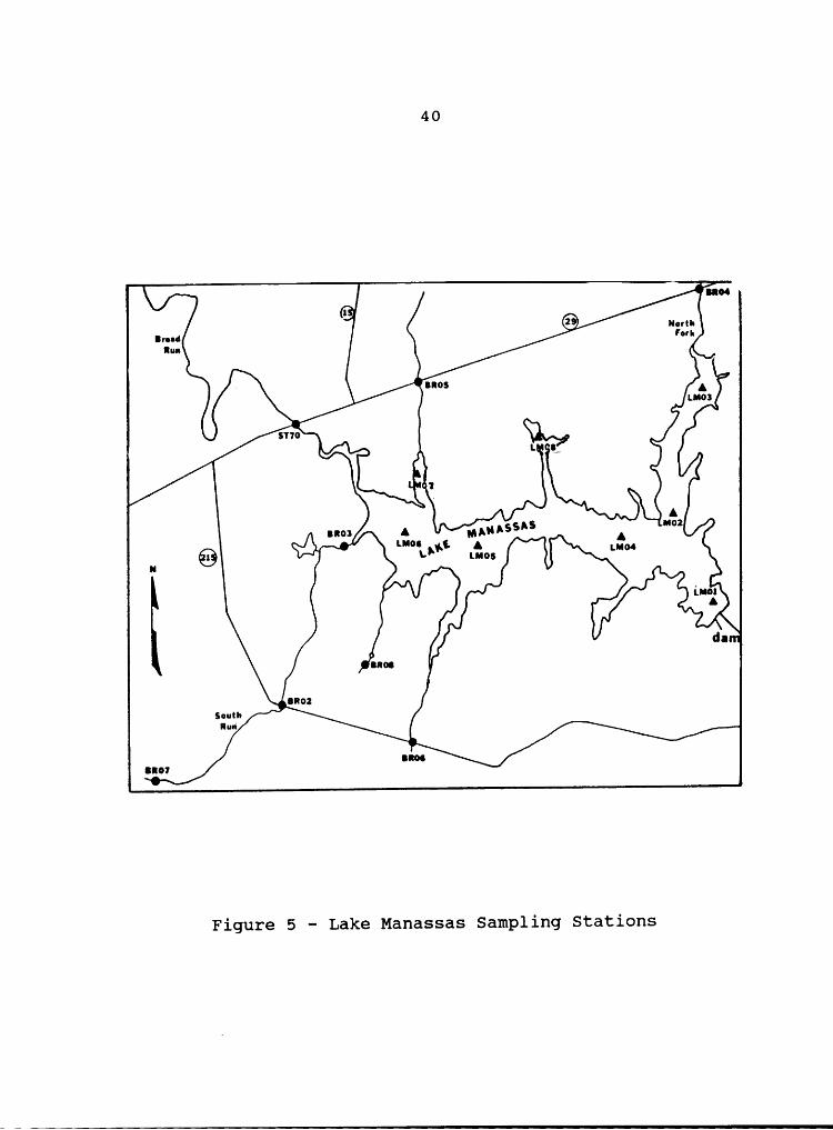
Figure 5 - Lake Manassas Sampling Stations ....... 40

Figure 6 - Hypsographic Curve for Lake Manassas ..... 57

Figure 7 - Temperature Profile at Monitoring Station —

LMO1 ..................... 59

Figure 8 - Temperature Profile at Monitoring Station

LM02 ..................... 60

Figure 9 - Temperature Profile at Monitoring Station

LM03 ..................... 61

Figure 10 — Temperature Profile at Monitoring Station

LM04 .....................62Figure11 - Temperature Profile at Monitoring Station

I

LM05 ..................... 63

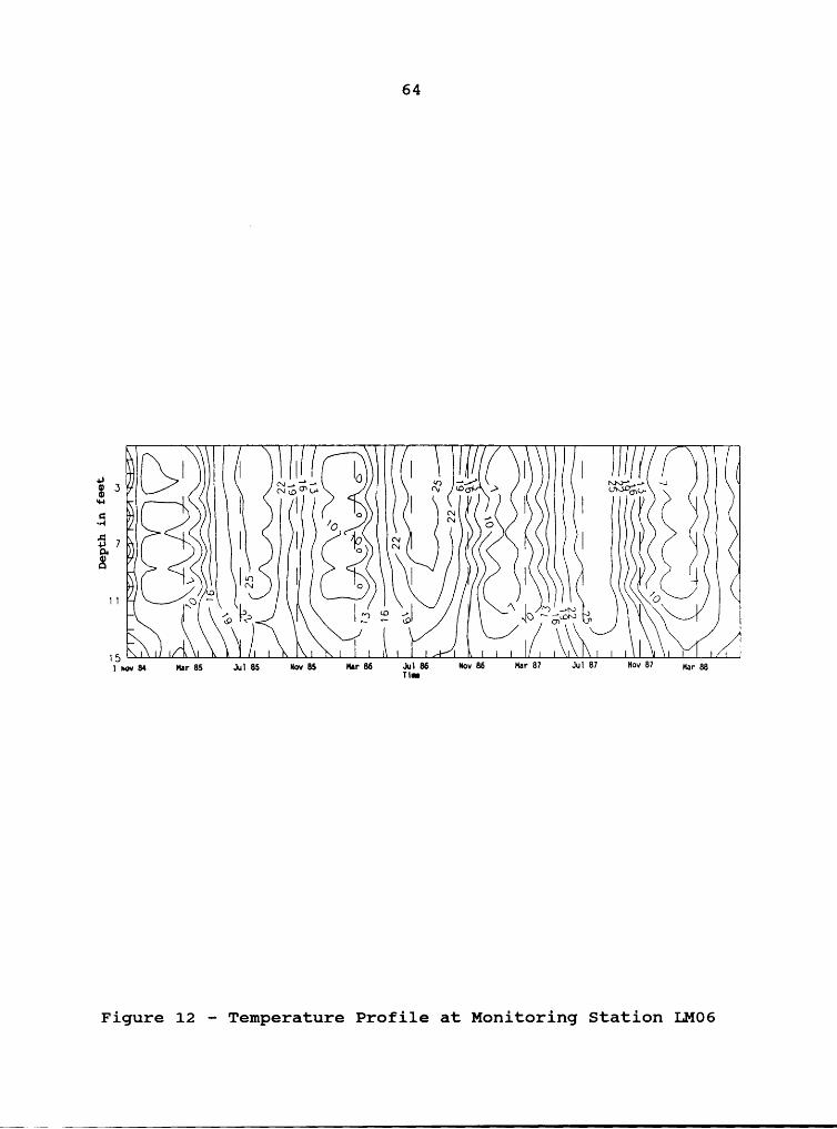
Figure 12 — Temperature Profile at Monitoring Station

LM06 ..................... 64

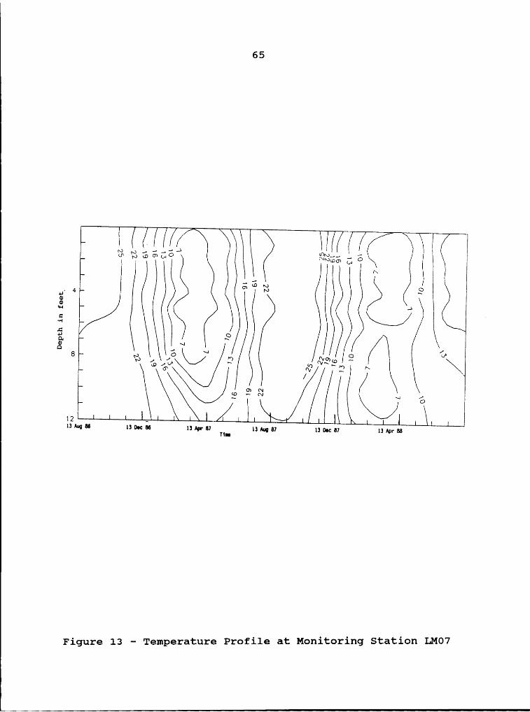
Figure 13 - Temperature Profile at Monitoring Station

LM07 ..................... 65

Figure 14 - Temperature Profile at Monitoring Station

LM08 ..................... 66

Ivii I

Lee............................................_....____________________

Figure 15 - Dissolved Oxygen Profile at Station LMO1 . . .68

Figure 16 — Dissolved Oxygen Profile at Station LMO2 . . .69

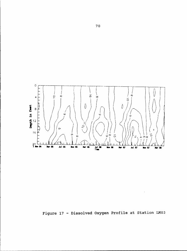
Figure 17 - Dissolved Oxygen Profile at Station LM03 . . .70

Figure 18 — Dissolved Oxygen Profile at Station LMO4 . . .71

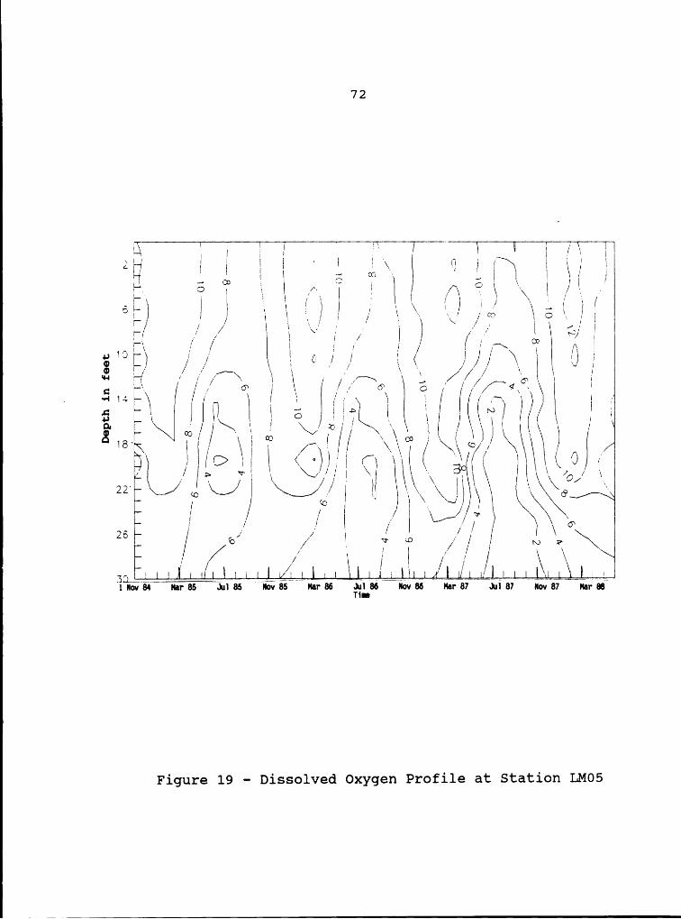
Figure 19 — Dissolved Oxygen Profile at Station LM05 . . .72

Figure 20 - Dissolved Oxygen Profile at Station LMO6 . . .73

Figure 21 — Dissolved Oxygen Profile at Station LM07 . . .74

Figure 22 — Dissolved Oxygen Profile at Station LM08 . . .75

Figure 23 — % Saturation DO Profile at Station LM01 . . .77

Figure 24 - % Saturation DO Profile at Station LMO2 . . .77

Figure 25 - % Saturation DO Profile at Station LM03 . . .78

Figure 27 - % Saturation DO Profile at Station LMO4 . . .79

Figure 27 — % Saturation DO Profile at Station LM05 . . .80

Figure 28 - % Saturation DO Profile at Station LM07 . . .81

Figure 29 - % Saturation DO Profile at Station LM07 . . .82

Figure 30 - % Saturation DO Profile at Station LM08 . . .83l

Figure 31 - Top and Bottom DO Profiles at Station LM01 . .85

Figure 32 - Top and Bottom % Saturation DO Profiles

at Station LMO1 ...............86

Figure 33 - Top and Bottom DO Profiles at Station LM08 . .87

Figure 34 — Top and Bottom % Saturation DO Profiles

at Station LM08 ...............88

Figure 35 — Chlorophyll Q Profile at LMO1 ........90

Figure 36 — Chlorophyll Q Profile at LMO2 ........91

viii

I

tFigure 37 — Chlorophyll Q Profile at LMO3 ........92

Figure 38 - Chlorophyll Q Profile at LM06 ........93

Figure 39 - Chlorophyll Q Profile at LMO7 ........94

Figure 40 - Chlorophyll Q Profile at LMO1 & LM02 .....95

Figure 41 - Chlorophyll Q Profile at LMO3 & LM07 .....96

Figure 42 - Chlorophyll Q Profile at LMO3 & LMO7 .....97

Figure 43 — Surface Chlorophyll Q at LMO1 and LM03 ....99

Figure 44 — Surface Chlorophyll Q at LMO1 and LM07 . . . 100

Figure 45 — Surface Chlorophyll Q at LMO7 and LM07 . . . 101

Figure 46 — Nitrogen in the Bottom Waters of LMO1 . . . 103

Figure 47 — Nitrogen in the Bottom Waters of LMO7 . . . 104l

Figure 48 - Nitrogen in the Bottom Waters of LM07 . . . 105

Figure 49 — Oxidized Nitrogen at the Top and Bottom

of LMO1 ...................106

Figure 50 — Nitrogen and Phosphorus at the Bottom

of LMO1 ...................108

Figure 51 - Nitrogen and Phosphorus at the Bottom

of LMO7 ...................109

Figure 52 - Phosphorus in the Bottom Waters at LMO1. . . 110

Figure 53 — Phosphorus in the Bottom Waters at LMO7. . . 111

Figure 54 - Total Phosphorus in the Surface at LMO1, LMO3

and LMO7 .................. 112

Figure 55 — Rainfall in Lake Manassas watershed .... 115

ix

IFigure 56 - % Runoff into Broad Run versus Yearly

Rainfall .................. 116

Figure 57 - ST70 Loading of Orthophosphorus ...... 123

Figure 58 - ST70 Loading of Total Soluble Phosphorus . . 124

Figure 59 - ST70 Loading of Total Phosphorus ...... 125

Figure 60 - ST70 Loading of Ammonia Nitrogen ...... 126

Figure 61 — ST70 Loading of Oxidized Nitrogen ..... 127

Figure 62 — ST70 Loading of TKN ............ 128

Figure 63 - ST70 Loading of SKN ............ 129

Figure 64 - Spreadsheet Statistical Model for

Lake Manassas ............... 131

Figure 65 - Current Average Phosphorus Loading ..... 132

Figure 66 - Current Median Phosphorus Loading ..... 133

Figure 67 - CURAVGLOAD Output Distribution Graph .... 134

Figure 68 - CURMEDLOAD Output Distribution Graph .... 135

Figure 69 - Vollenweider Plot of Current Conditions in Lake

Manassas .................. 136i

Figure 70 — Vollenweider Plot of Lake Manassas after

eliminating the Vint Hill point source

discharge ................. 139

x

WLIST OF TABLES

Table 1 - Nutritional Requirements ...........26

Table 2 - Carlson's Trophic State Index ........36

Table 3 - Trophic State Indices based on Chlorophyll Q .37

Table 4 - EPA Trophic State Index System ........38

Table 5 - Distribution Functions for Spreadsheet Model .47

Table 6 — Database Structure and Contents .......51

Table 7 - Morphological Characteristics of Lake

Manassas ...................56

Table 8 — Properties of Lake Manassas Watershed Basins 114

Table 9 · Summary of Environmental Monitoring Data for

Drainages into Lake Manassas ........ 118

Table 10 — Summary of Metal Content of Drainages to Lake

Manassas .................. 120

Table 11 — Summary of Results from Spreadsheet Model of

Lake Manassas ............... 138

Table 12 - Summary of Other Trophic State Indices for Lake

Manassas .................. 141

xi

IChapter I

INTRODUCTION

Groundwater became an undependable supply of potable

water in the area around the City of Manassas, Virginia, in

the mid—1960·s. The expanding population increased the

demand for water to the point where the aquifer experienced

an overdraft condition. Because the population was expected

to continue to increase at a relatively rapid rate, the

overdraft condition would continue to worsen.

In response to this problem, the City of Manassas began

a study for alternative supplies of water. The result of

this study was the recommended development of a man·made

impoundment, Lake Manassas, by constructing a dam on Broad

Run, approximately 10 miles west of the City of Manassas.

In 1968 the construction process began and by 1971 the lake

and a new water treatment plant were supplying water to the

City of Manassas.

The lake was designed for a capacity of 5.8 billion

gallons and a surface area of approximately 780 acres.

However, more recent studies indicate these design figures

may be ten to twenty percent higher than the actual size of

the lake. The issue of lake size, will be discussed in

1

I

2 4

subsequent sections of this report. The water treatment

plant was initially designed for a capacity of 4 million

gallons per day (MGD), but the continued expansion of the

surrounding population necessitated a doubling of the output

capacity to 8 MGD in 1987. Figure 1 shows the location of

Lake Manassas in the north-eastern corner of Virginia,

approximately 30 miles due west of Washington, D.C.

Lake Manassas lies in the upper reaches of a major

watershed for Northern Virginia: the Occoquan River

watershed. The Occoquan River is impounded by a dam near

its discharge into the Potomac River, south of Washington,

DC. The Occoquan Reservoir is one of the largest potable

water reservoirs in the northern Virginia area. Because of

this, the Occoquan Reservoir and its watershed have been

monitored and studied extensively.

Lake Manassas has grown in popularity as a recreational

facility since its construction. The lake is stocked with

fish, and the State Game Commission allows access to the

lake for fishing on a permitted basis. No gasoline engines

are allowed on the lake, and no swimming is permitted. A

further example of the popularity of the lake is the recent

acquisition of a significant portion of the land on the

north—western shoreline for construction of a large golf

resort and convention center. Current plans include the

El

3

Reservolr

derrun

Figure 1 - Geographic Location of Lake Manassas

4

construction of three 18 hole golf courses, and an

accompanying hotel and convention facility.

Limnological principles show that as the development of

a watershed proceeds, the increased input of nutrients and

other pollutants results in the gradual decline of the

quality of the receiving water body. This decline is

typified by an increase in algal growth, known as lake

productivity. Typically, taste and odor problems and

filtration overloading, all caused by these microorganisms,

make it difficult and uneconomical to treat the water. Asl

the lake productivity continues to increase, the water body

can no longer be a useful supply of potable water. However,

there are land management practices that can be implemented

to minimize or control this undesirable environmental

process.

It can be expected that as the population of this

geographic region continues to increase, there will be an

accompanying increased demand for potable water. Therefore,

it is important that all existing water supply resources

continue to be protected from any decline in quality.

The objectives of this study are to present a

comprehensive analysis of the existing conditions in Lake

Manassas. These existing, or baseline, conditions can be

used in a comparative fashion to track the changes in the

5

lake as the watershed development continues. These

comparisons can be a useful way to monitor land management

practices in the watershed so that their maximum

effectiveness is achieved.

Specific objectives of this study were (1) to

investigate the limnological characteristics of Lake

Manassas including the morphology, stratification due to

thermal effects, nutrient input and distribution, and lake

productivity; (2) to use existing models to predict the

magnitude of eutrophication in the lake; and (3) to

characterize the major input streams to the lake.

1Chapter II

LITERATURE REVIEW

History of Lake Manassas

Lake History

In 1962, the Town Council of Manassas requested that

I the Northern Virginia Soil Conservation District make a

survey of possible sites for a water reservoir that would

replace the increasingly unreliable groundwater supply. The

community was undergoing rapid development, and the

overdraft condition in the aquifer would only worsen with

time. The survey proposed the development of an impoundment

on Broad Run by placing a dam just south of the confluence

of Broad Run and the North Fork tributary to Broad Run. The

land in this area was purchased, and a bond referendum

provided the funds to construct the dam. (1) Construction

began in November of 1968, and the dam was completed in

1970. Parallel with construction of the dam, a water

treatment plant at the base of the dam was designed and

constructed. The treatment plant began supplying water in

1971 to the City of Manassas through a seven mile long, 24-

inch diameter water main (2).

6

7

Water Treatment

The water treatment plant was initially designed to

operate at a capacity of 4 MGD, and did so until 1987 when a

plant expansion doubled its capacity to 8 MGD. Currently,

the plant is operating at a nominal capacity of 6.7 MGD

supplying water to the City of Manassas, and to the Prince

William County Service Authority for other areas of Prince

William County, Virginia. In addition to this withdrawal of

water from Lake Manassas, a small hydroelectric plant at the

base of the spillway was completed in 1987. This

hydroelectric plant is designed to supplement local peak

electricity demand. The hydroelectric plant is therefore

only operated intermittently. Current plans are to operate

the hydroelectric plant 3 to 7 hours per day, 5 to 10 days

per year. (2)

Raw water is withdrawn from the lake by an intake

system at depths of 5, 15, 25, 35, 45, and 55 feet below the

lake surface. The spillway elevation of the lake is 285

feet above sea level. Typically, all water is drawn from

the 5-foot level except during summer when some water is

drawn from the 15—foot level and mixed with the shallower

water to achieve an acceptable temperature. Deeper water is

rarely withdrawn because experience has shown that the

higher level of dissolved iron and manganese of the deeper

8

waters causes processing problems. The water is then

conveyed via an underground pipeline to the treatment plant.

Pumps are available to pump water from the lake, but normal

lake levels provide sufficient head for gravity flow. The

raw water enters the plant in a rapid mix chamber where

typically, the following chemicals are added; potassium

permanganate for oxidizing iron and manganese, liquid alum

to enhance flocculation, caustic soda for pH control,

hydrofluorous salaic acid for fluoridation purposes,

hexametaphosphate for corrosion protection, and some gaseous

chlorine for preliminary disinfection. After the mix

chamber, the water is sent to one of the two identical

processing systems to complete treatment. (The plant

expansion of 1987 essentially built an identical processing

system parallel to the existing system.) The water flows

through a series of settling basins which contain rotating

flocculators to enhance flocculation and settling. The

water then flows into dual media filters consisting of a bed

of granular activated carbon (GAC) overlying sand. GAC is

used because of problems with taste and odor control. The

water from Lake Manassas has had taste and odor problems

since the opening of the reservoir. As a historical note,

this water treatment plant was the second facility in the

State of Virginia to use GAC for taste and odor control. (2)

9

Finished water is held in one of two 205,000 gallon

clearwells, which form the structural foundation of the

water treatment plant buildings. The water is then

withdrawn from the clearwells, and pumped into a 24-inch

main which carries the water to water tanks nearer the city.

To complete the disinfection process, and to provide the

necessary chlorine residual for the distribution system,

gaseous chlorine is added just before the water enters the

main.l

Treatment plant operators have been experimenting by

varying chemical addition rates to reduce the level of

trihalomethanes (THM's) produced by the chlorination

process. In general, the THM production level is controlled

by the amount of pretreatment chlorination. Some

experiments have shown that with minimal pretreatment

chlorination, the level of THM's leaving the plant can be

maintained below 30 parts per billion. (2) Current drinking

water regulations require THM's to be held to less than 100

parts per billion.Algae from Lake Manassas have historically caused

significant processing problems. Filter clogging was very

predominant, as were taste and odor problems. In order to

control these problems, Lake Manassas is treated with copper

l

I10

sulfate, an algicide. The copper sulfate is applied from a

moving boat in powder form and is typically applied four

times per year, twice in the spring and twice in the fall.

The application of copper sulfate to Lake Manassas has been

practiced for approximately 14 years. (2)

The water from Lake Manassas is rather soft, with an

average total hardness of less that 40 milligrams per liter

(mg/L) as calcium carbonate (CaCOg. Therefore, the

treatment plant does not perform any processing for hardness

reduction.

Watershed Management

As previously stated, Lake Manassas and its watershed

are part of the larger Occoquan River watershed. The

Occoquan River is impounded by a dam near its outlet into

the Potomac River. The Occoquan Reservoir is a very

important water resource in the Northern Virginia area

because it supplies potable water to over 750,000 people and

regional businesses (3).

In 1971, the Commonwealth of Virginia State Water

Control Board issued a policy statement titled "waste

Treatment and Water Quality Management in the Occoquan

Watershed" (3). This policy statement was the result of

research into the increasing pollution content of the

——9e———————————-—------.....................,.___________________________

11

Occoquan Reservoir. In the early 1970's, the major sources

of pollution into the watershed were point source discharges

from sewage treatment plants. The new policy statement

instituted the following major programs:

1. New high-performance wastewater treatment

facilities in the watershed were to be constructed

to replace some of the existing low efficiency

plants.

2. The Occoquan watershed Monitoring Program was

established to continue to monitor the water

quality of the reservoir and its watershed.

3. Erosion and sediment control standards were

invoked.

The State Water Control Board revised the Occoquan watershed

Policy in 1980 to include more detailed requirements for the

performance of new treatment plants and the expansion of

existing treatment plants in the watershed (3). Most of the

analytical data used in this document were obtained from the

Occoquan watershed Monitoring Program.

Current Watershed Development

In November, 1985, a golf resort development company

requested permission from the Prince William County,

Virginia, Planning Commission to build a golf resort on the

I

12

northern shores of Lake Manassas. The golf resort plans

include golf courses, 800,000 square feet of office space, a

500 unit full service hotel, and a residential community of

400 detached single family homes, 200 condominium homes, and

200 townhouse homes. (4) The placement of this resort is

shown in Figure 2, with the golf courses nearest to the lake

areas.

The land that the resort would be placed on is

essentially undeveloped forest and pasture land with minimal

population currently present. In order to obtain a

preliminary understanding of the potential impact this

resort community may have on Lake Manassas, the Prince

William County Planning Commission contracted with the

Northern Virginia Planning District Commission for a

technical analysis. In April of 1986, the Planning District

Commission published the results of their analysis (5). The

following statements summarize the qualitative results of

the analysis;

"Results of the Watershed Model simulations showedthat, due to the very small size of the site [theproposed resort] compared to the total area thatdrains to Lake Manassas, the proposed developmentwould have only a slight effect on the lake. Thefact that the model showed any effect at all,however, indicates that additional developmentwithin the watershed without adequate controlscould result in significant adverse impacts onwater quality in the lake." (5)

That report also recommended that runoff control measures

I

13

and structures be built around the proposed resort to

minimize nutrient and pollutant loadings into Lake

Manassas (5).

K

14

‘ oAan 4 , ’I

.„-·i==E==EE===E==E===E==§:=¤zi -4nz!••§••l•••:§••=••:i¤•§••:=y'

I-!j··=·-=l·‘---···-=¢-=|-=-lg

;•¢-nl,••·•¤=•••!••:•¤l••:••*'

jl glljl I=l°

wir

„ @3

Ruvi

Figure 2 - Development of the Lake Manassas Watershed

15

Limnological Principles

The Lake as an Ecosystem

The study of fresh water bodies, their ecosystems, and

their response to environmental changes is termed limnology.

Limnology is a complex discipline because of the dynamic and

extreme diversity of conditions that exist in the freshwater

bodies of the world. Lakes are ecosystems with the

metabolism of the resident species (herein termed a lake's

metabolism) dependent on and responsive to the inputs of the

entire drainage basin of the lake, the atmosphere, and the

sun(6). As with any scientific discipline, there are

"yardsticks" which have been developed to measure parameters

and thereby enable comparisons between different lakes.

These parameters will be presented along with a discussion

of their effects on a lake.

Morphology

The size and shape of a lake is highly dependent on the

mechanism by which the lake was created (6). Examples of

the processes which create freshwater lakes include:

tectonic movement resulting in the creation of huge basins,

volcanic activity which produce lava flows that can distort

1A——A—-—-—-e---—.-..................................._._„___________Q

Ä

16Ä

as they cool to form cavities and dams, landslides which

create natural dams in existing drainage pathways, glacial

activities which carve out earthen soil and bedrock and

subsequently deposit these materials as dams when the

glaciers recede, meandering rivers which can have entire

sections cut off by sedimentation processes, solution lakes

caused by the dissolution of certain bedrock, shoreline

lakes which result from the cyclic erosion and deposition

actions of wave activity, and manmade lakes which are often

formed by damming existing drainage ways. (7)

Examples of parameters which are used to describe the

morphological characteristics of a lake include lake area:

lake volume, maximum, mean, and relative depths, lake

length, shoreline length, and shoreline development. The

final term, shoreline development, is defined as the ratio

of a lake's shoreline length to the radius of a circle whose

area is that of the lake. Therefore, a perfectly circular

lake would have a shoreline development of 1.00. Typically,

natural lakes have a shoreline development of around 2.00

with some manmade impoundments approaching a value of

5.0 (6). Shoreline development is of interest because it

reflects the potential for greater development of littoral

communities (shallow shoreline areas with a higher

preponderance of life forms) in proportion to the volume of

Ä

17

the lake (8).

The volume of a lake is an important parameter because

it controls the concentration of constituents within the

lake and therefore the lake's metabolism. These data are

often presented in the form of a hypsographic curve which

plots the depth of a lake versus the percent of the total

lake area for a particular depth. The shape of this curve

can help indicate whether a lake has a substantial portion

of its volume at a depth where light could penetrate and

provide energy for photosynthetic organisms (9).

Hydraulic retention time, or the average time an

individual water molecule spends in a lake, is a useful

parameter to relate a lake to its surrounding drainage

basin. Long retention times indicate a stable lake

metabolism, and short retention times indicate a propensity

for quick changes in lake metabolism due to rapid changes in

lake inputs. (6)

Energy Input to Lakes

A lake's metabolism is highly dependent on the input

and distribution of energy within the lake. The food chain,

be it terrestrial or aquatic, starts with the conversion of

solar energy into chemical energy via the process of

photosynthesis. Furthermore, most life forms need some form

18

of thermal energy to keep their temperature in the range

necessary for biochemical processes to proceed. Therefore,

the amount of light impinging on a lake, the depth to which

it penetrates, and the overall distribution of the resulting

thermal energy is very important to a lake's metabolism.

(6,9)There is an array of physical, chemical, and biological

properties which controls the absorption of solar energy.

However, it is the distribution of this energy that is of

most interest to limnological studies. As water becomes

warmer, it also becomes less dense and therefore rises to

the surface of the lake. The cooler, more dense water sinks

and remains in the deeper portions of the lake. Figure 3

represents the change in the density of water with

temperature. Other forces on the lake, such as wind, tend

to promote mixing. However, during the spring and summer

months, the heat input from solar radiation, and the often

less windy conditions associated with the warmer seasons,

create conditions where the heat induced density gradient

remains quite evident, a condition known as stratification.

The layer of warmer water on the top of the lake is termed

the epilimnion, the layer with a relatively rapid

temperature change with depth is termed the metalimnion, and

the lower layer of colder water the hypolimnion. It is

19

‘ , - · — — _ _ 0.01‘ ~ X 0.006

0.999 ‘ X x \ O;\ \V0 xE ¤ OU \ — .005Ö \E 0.998 ‘ 2.\ ‘

X -0.01 g\/\ Cs. \ °°

2 x *0.015 glO x; 0.997 X g‘X -0.02 Rlv; xC \Q \C! -0.025

\\\

-0.03

0.995010 zu 30_ _ Temperature In degree: CDWWHY “' % Change in Density

Figure 3 — Density of Water versus Water Temperature

1

20

easily seen that this set of conditions also acts as a

barrier to mixing of dissolved materials between the layers

of different density (6,9). The effects of this

stratification will be developed further in later

discussion.

With a change in seasons (summer to autumn), the

epilimnion cools to a point where it's density is no longer

significantly different from the rest of the lake. At that

time, the action of wind can induce sufficient mixing action

to create a condition known as turnover. The hypolimnion

and its dissolved materials then mix with the rest of the

lake to create essentially uniform chemical conditions

throughout the lake. (10)

Depending on the climate of the lake's location, ice

can form in winter. The ice cover then creates a small

thermal gradient near the surface of the lake. However,

this stratification condition is much less severe than the

summer stratification. (6, 9)

With the onset of spring, the uniform temperature

gradient develops again and spring turnover occurs. As the

heat input of solar radiation increases in the spring, the

entire stratification cycle is then repeated. A lake which

experiences this type of repeated cycle is termed a dimictic

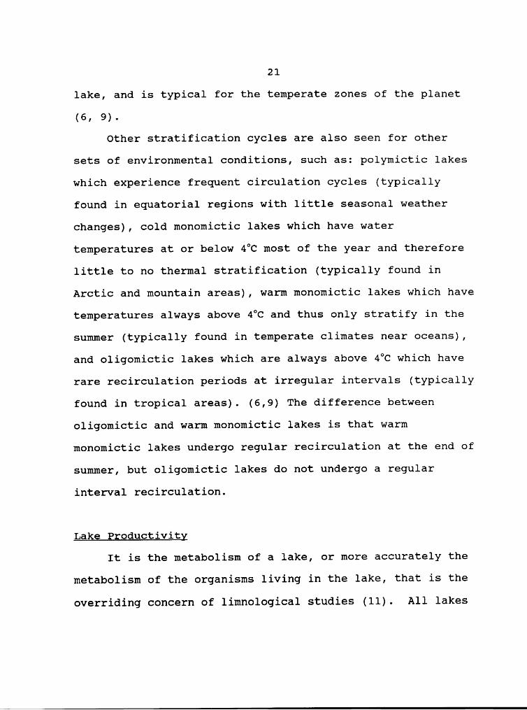
21

lake, and is typical for the temperate zones of the planet

(6, 9).

Other stratification cycles are also seen for other

sets of environmental conditions, such as: polymictic lakes

which experience frequent circulation cycles (typically

found in equatorial regions with little seasonal weather

changes), cold monomictic lakes which have water

temperatures at or below 4FC most of the year and therefore

little to no thermal stratification (typically found in

Arctic and mountain areas), warm monomictic lakes which have

temperatures always above 4%Zand thus only stratify in the

summer (typically found in temperate climates near oceans),

and oligomictic lakes which are always above ¢© which have

rare recirculation periods at irregular intervals (typically

found in tropical areas). (6,9) The difference between

oligomictic and warm monomictic lakes is that warm

monomictic lakes undergo regular recirculation at the end of

summer, but oligomictic lakes do not undergo a regular

interval recirculation.

Lake Productivity

It is the metabolism of a lake, or more accurately the

metabolism of the organisms living in the lake, that is the

overriding concern of limnological studies (11). All lakes

22

will go through a gradual process of building up sedimentary

material, ultimately turning the lake into a soil column

with surface water flowing over it (6, 9, 11). This process

is called eutrophication. Some sedimentary material is

always being added from the entrained sediment in the supply

waters to the lake. However, depending on the propensity

for organic life forms to exist in the lake, the buildup of

the sediment may be much more rapid due to the addition of

detritus from dead organisms. The usefulness and aesthetic

qualities of the lake may also be severely impacted if too

much organic life is present. For example, excessive algae

growth makes the water difficult to treat for domestic use,

and can inhibit recreational use of the lake (12).

Therefore, it is the productivity of new biomass within the

lake (its metabolism) that can drastically affect the useful

lifetime of a lake (13). It is important at this point to

ensure a useful terminology and technical approach is

developed for this study. The underlined text in the

following quote was added by the author of this thesis to

emphasize key concepts.

"Much of the confusion ...[of limnology]... emanatesfrom early concepts that considered productivity as themaximum growth and development of organisms underoptimal conditions. While the potential of organismsto produce and increase towards infinity may be auseful conceptual framework, in the real worldenvironmental constraints regulate these increases.Optimal conditions for an organism, population,community, or ecosystem can, at best, only be

23i

approximated after extensive investigation. ... It ismuch more meaningful to define the terms production andproductivity in relation to realized or actualproduction of organisms. Changes in production arerelated ...[to the]... dynamics of environmental ...parameters." (6)

It is the environmental parameters such as oxygen content

and nutrient availability, and their affects on lake

organisms that will be discussed further in this study.

This author does not intend that the above noted quotation

over simplify limnology. Instead this author intends that

the quotation help focus the scope of this study because

limnology can involve so many complex interactive variables.

A lake that is low in biomass productivity is termed

oligotrophic, and this condition most often corresponds to a

low supply of nutrients for organic life. As the nutrient

supply slowly increases, so does the biomass productivity

and the lake becomes mesotrophic. Finally, a lake which is

enriched in nutrients to a point where other parameters,

such as the length of the warm season, control the biomass

production is termed eutrophic (14).

Typically, the algal population in a eutrophic lake is

high during the spring and summer seasons because there is

adequate sunlight and because of the slower metabolism rate

during the cooler seasons (9). Algae produce oxygen during

photosynthesis, and it is quite common for the epilimnion

uu

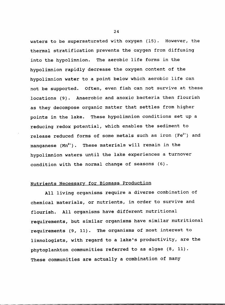
2 4 *waters to be supersaturated with oxygen (15). However, the

thermal stratification prevents the oxygen from diffusing

into the hypolimnion. The aerobic life forms in the

hypolimnion rapidly decrease the oxygen content of the

hypolimnion water to a point below which aerobic life can

not be supported. Often, even fish can not survive at these

locations (9). Anaerobic and anoxic bacteria then flourish

as they decompose organic matter that settles from higher

points in the lake. These hypolimnion conditions set up a

reducing redox potential, which enables the sediment toV

release reduced forms of some metals such as iron (Fe”) and

manganese (Mn”). These materials will remain in the

hypolimnion waters until the lake experiences a turnover

condition with the normal change of seasons (6).

Nutrients Necessary for Biomass Production

All living organisms require a diverse combination of

chemical materials, or nutrients, in order to survive and

flourish. All organisms have different nutritional

requirements, but similar organisms have similar nutritional

requirements (9, 11). The organisms of most interest to

limnologists, with regard to a lake's productivity, are the

phytoplankton communities referred to as algae (8, 11).

These communities are actually a combination of many

N

N25

individual microbiological algae species, including the

blue—green, green, yellow-green, red, brown, and golden-

brown algae, as well as the diatoms and euglenoids. These

organisms are photosynthetic, converting sunlight into

chemical energy for their entire biochemical metabolism.

Table 1 lists their basic nutritional needs and the sources

of the nutrients (1, 6).

Studies have shown that the average stoichiometric

cellular makeup of freshwater algae organisms is given by

C„H„5%J%P (16). From this molecular formula, and the

biological data of Table 1, some conclusions can be made

regarding the nutritional requirements of freshwater algae.

First, carbon, hydrogen, and oxygen are needed in relatively

large amounts for production of cellular biomass. Second,

nitrogen and phosphorus are also needed but in lesser

amounts.

A parallel concept concerning nutritional requirements

and organism productivity is Leibig's "Law of the Minimum"

(9). In 1840, Justus Leibig, while studying inorganic

chemical fertilizers, found that crop growth was limited by

whatever essential element was in shortest supply,

regardless of whether the total amount required was large or

small (1). Therefore, whatever nutrient is the

l

l

26

Table 1 - Nutritional Requirements(6)

Function Source

Energy Source Organic and inorganic compoundsSunlight via photosynthesis

Electron Acceptor O2from Respiration Organic compounds

NO; , NO2” , so}Material for CO2,.HCO;, NOg, NO;, PO;2Cellular Biomass Organic compounds

Trace elements such as vitamins

27 lleast abundant, relative to an organism's need, is the

controlling nutrient for organism productivity.

This concept is a useful and well proven predictive

tool for limnologists and many other biological scientists

(6, 9, 10, 14). However, it should be emphasized that it is

a "relative law", subject to the level of detail of the

. analysis. For example, certain vitamins may be essential to

an organism‘s biochemical pathways such that its absence,

regardless of the supply of energy sources and electron

receptors, could prevent that organism from flourishing.

Also, as stated previously, the dynamic change in the

characteristics of environmental parameters, including

nutrients, also affect the productivity of lake ecosystems.

In lakes, the most necessary chemical elements are also

the most prolific. Carbon is readily available from organic

matter present, CO2, and the dissolved forms of CO2 HCO2 and

cofx Hydrogen is readily available from organic matter

present and water itself. Oxygen is reasonably available in

the epilimnion from both dissolved atmospheric O2, and O2

produced from the photosynthesis process (6). For aerobic

life forms, oxygen is the terminal electron acceptor in

biochemical oxidation - the energy producing process. In

anaerobic and anoxic life forms, other compounds can be the

terminal electron acceptors. Since carbon, hydrogen, and

I28

oxygen are available in relatively large amounts, the

availability of nitrogen and phosphorus controls the

production of algae.

In summary, nutrients can be kinetically or

stoichiometrically limiting. Although the assumptions for

deriving limiting nutrients under either of these categories

can be different, both should be considered when performing

such analyses (10).

The above analysis stresses the production of algae and

other similar biomass. This does not mean that in other

areas of the lake different biochemical processes (or

metabolic pathways) result in a prolific collection of

different life forms, such as anoxic and anaerobic bacteria

in lake sediment (6, 9). However, these other metabolic

pathways are not as efficient in the production of biomass

material (17).

Nitrogen is a common element in the environment, and

its availability to freshwater lakes is the result of

numerous sources. Limnological studies have yielded the

following information regarding some of the pathways in a

lake's nitrogen budget (6, 8, 9, 10, 14).

1. Aerobic decomposition processes are not present in

an anaerobic hypolimnion.

Z29

2. The metabolism of epilimnion organisms can be a

major source of organic nitrogen in lakes.

3. Many components of nitrogen input to lakes are

either seasonal or intermittent in application and

variable in magnitude. Examples of these sources

include organic and ammonia nitrogen from water fowl

excretions, and both organic and oxidized nitrogen from

sewage treatment plant discharges.

4. Nitrogen uptake and release from sediments is a

complex and not well understood process. One study

showed that although there is a significant source of

nitrogen present in lake sediments, it is not readily

available for metabolism in a lake system. Therefore,

I the influent sources of nitrogen usually determine the

quantity of nitrogen available in the water column of a

lake.

In summary, for most lakes, nitrogen is available in

sufficient quantities to not be the limiting nutrient for

algae growth. However, because nitrogen is critical for

biomass production, the amount of nitrogen present can have

w

30

an affect upon the total amount of biomass produced.

Therefore, minimizing the nitrogen input to a lake is still

a desirable objective.

The magnitude of nitrogen in drinking water can also be

an environmental health issue (18). Ammonia is toxic to

many organisms when present in sufficient quantities, and

nitrate is toxic to human infants (19). Therefore, control

of nitrogen is important for both lake productivity and

water resource usefulness.

The preceding discussion concludes that phosphorus is

often the most kinetically and/or stoichiometrically

limiting nutrient with respect to lake productivity. This

has been demonstrated in numerous laboratory and natural

environmental experiments. For example, one of the most

dramatic experiments was performed on a natural lake in

Ontario, Canada, which had a natural shape like a dumbbell

(6). A partition was placed in the narrow section connecting

the lobes of the lake. The partition prevented cross-flow

between the two main lobes of the lake. One lobe was

fertilized with phosphorus, nitrogen, and carbon, and the

other lobe was fertilized with equivalent concentrations of

nitrogen and carbon only. Algal biomass increased two

orders of magnitude in the lobe which received the

phosphorus, but it did not appreciably change from normal

1

V

31}

conditions in the other side. (6) Pre-experiment conditions

returned in both lobes of the lake quickly after

fertilization was stopped. Many other similar experiments

demonstrate that phosphorus inputs to a lake ecosystem can

drastically and rapidly change the biomass production rate

(20).

Most of the phosphorus (often greater than 95 percent

by mass) present in a lake at any time is not readily

available for utilization by algae (11). This unavailable

phosphorus is bound in organic phosphates and cellular

constituents of organisms, both living and dead, and is

absorbed by organic and inorganic colloids, and particulate

compounds (6). Also, the highly reactive chemical

properties of phosphorus further amplify the shortage of

this nutrient, because any supply is rapidly depleted (9).

Phosphorus exchange between lake water and sediment is

highly dependent on the oxidation-reduction conditions at

the sediment water interface, and on the mixing (turbulence)

conditions of the lake (21). In general, studies have shown

that the phosphorus budget of a lake is more complex than

the nitrogen budget, partly due to the rapid kinetics of the

phosphorus reactions which make measurements difficult (6).

32

Quantification and Prediction of Lake Productivity

The ability to quantify and predict the trophic status

of a lake can be useful when it is desired to monitor,

control, or correct the productive status of a lake (10,

14). Numerous models have been developed which insert

easily measured parameters into empirically developed

relationships. Most of these models have been developed

based on the assumption that a lake is phosphorus limited.

Since these models are empirically developed, their results

must be tempered with appropriate professional judgement

(6)-One of the first and most successful models developed

was the Vollenweider model (6, 20). This model used annual

mean concentration values of total phosphorus and

chlorophyll a to assign a trophic status to a lake.

Vollenweider then improved his model to use the annual

loading rates of phosphorus to arrive at a trophic status.

It is then easier to develop control measures to ensure

loading rates do not exceed the desired level of

productivity.The Vollenweider model is a mass balance equation for

phosphorus. The change in total phosphorus is equal to the

influent loading of phosphorus minus the sum of the outflow

of phosphorus and the sedimentation of phosphorus. The data

I

Z2 2 *

are represented by graphing the annual phosphorus loading

(mass/area/time) versus the mean depth (length) times the

hydraulic retention time (years). The abscissa in this

graph is the relative "flushing" term because it relates the

rate at which water is changed in the lake to the amount of

the lake which can produce algae due to light penetration.

The resulting curve is shown in Figure 4. Vollenweider

designated 'admissible' and °dangerous' loading levels,

which are depicted by the curves shown on Figure 4.

Vollenweider's assumptions were pointed out as

important limitations by Dillion (20); 1) the lake is well

mixed, thus ignoring stratification affects, 2) loading,

flushing, and sedimentation rates are constant, 3) the

sedimentation process is first order relative to the amount

of phosphorus present, and 4) no credit is taken for

internal loading of phosphorus.

A different type of model uses water transparency and

other parameters to arrive at a "trophic index".

In 1977, Carlson published a scheme to classify lakes

using three different Trophic State Indices (TSI) (22). He

emphasized that a TSI was not a water quality index, but

that the TSI could be useful for comparing lakes within a

region, and as a management tool for predicting productivity

34

10EUTROPHIC

Dongerous ///

Q3 /1

// //E // Perysséle9//E

/Q /P3 ,/"Ö

ii'-___-,••¢g 0.1 1o¤o,-1 0L1GO"1‘R01>1—11C

0.010.1 1 10 100

Medn Dep1n('Z)/Medn Residence T1nne(tdu)

Figure 4 - The Vollenweider Model Relatienship

E35

changes when it is used in conjunction with nutrient loading

concepts.

Carlson uses the epilimnion values of total phosphorus,

chlorophyll Q, and secchi disk reading to arrive at a TSI

for a lake. Carlson's scale is based on the increase in

algal biomass in response to an increase in the phosphorus

concentration. Many factors can affect the ability of

Carlson's model to accurately predict the trophic index of a

lake, such as seasonal changes, and highly colored or turbid

waters. He found that man—made impoundments showed

different relationships than did natural lakes. Carlson

speculated that man-made impoundments may be muddier than

natural lakes, thus affecting the secchi disk results. (1,

22)

Carlson's model yields a TSI value between 0 and 100.

However, he did not propose ranges of a TSI relative to the

older oligotrophic-mesotrophic-eutrophic system other than

to say that a higher TSI indicates an increased propensity

for eutrophic conditions.

Tables 2, 3, and 4 present the TSI scales developed by

Carlson, Sakamoto, Dobson, the National Academy of Sciences,

and the U.S. Environmental Protection Agency. The parameter

values provided are the epilimnion averages during the

summer season. (23)

A

36

Table 2 - Carlson's Trophic State Index (22)

Secchi Dish Surface SurfaceTSI Depth Total Phosphorus Chlorophyll Q

(m) (micrograms/liter) (micrograms/liter)

0 64 0.75 0.0410 32 1.5 0.1220 16 3.0 0.3430 8 6.0 0.9440 4 12 2.650 2 24 6.460 0.5 96 5670 0.5 96 15490 0.12 384 427100 0.062 768 1183

Analytical equations to generate the table given above are:

TSI Secchi (S) = 10*(6—(ln(S)/ln(2)))

TSI Total Phosphorus (TP) = 10*(6-(ln(48/TP)/ln(2)))

TSI Chlorophyll Q (Cha) = 10*(6·((2.04·0.68*lh(Cha))/1H(2))

i

\

137

Table 3 - Trophic State Indices Based on Chlorophyll QChorophyll Q in micrograms per liter (22)

TrophicCondition Sakamoto Academy Dobson EPA

Oligotrophic 0.3 to 2.5 0 to 4 0 to 4.3 <7

Mesotrophic 1 to 15 4 to 10 4.3 to 8.8 7 to 12

Eutrophic 5 to 140 >10 >8.8 >12

3 6 1I

Table 4 - EPA Trophic State Index System (22)

Trophic Chlorophyll a Total Phosphorus Secchi DishCondition (micrograms per liter) Depth (meters)

Oligotrophic <7 <1O >3.7

Mesotrophic 7 to 12 10 to 20 2 to 3.7

Eutrophic >12 >20 <2.0

I

Chapter III

METHODS AND MATERIALS

The City of Manassas has contracted with the Occoquan

Watershed Monitoring Laboratory (OWML), located in Manassas,

Virginia, to design and implement a monitoring program for

the lake and its tributaries (24). Sampling of the lake

began in October of 1984. Sampling of some of the

tributaries to the lake began as early as 1975 as part of

the greater Occoquan Watershed monitoring program. The OWML

has established schedules and procedures for the Lake

Manassas monitoring program, and the data generated from

this program is stored at the OWML and on the mainframe

computers of the Virginia Polytechnic Institute and State

University.

Sampling Program

The Lake Manassas sampling program consists of eight

sampling locations on the lake, and are designated on

Figure 5 as LMO1 to LMO8. The Lake Manassas tributary

monitoring program consists of eight sampling stations,

designated on Figure 5 as BRO2 to BRO8 and ST70. Samples

obtained at the stations denoted by the BR series are grab

samples, whereas samples from the ST70 station consist of

39

II

40

oe® NorthFork

IROS ‘’

LMO!

L L:

1

A

N

inno:A

t ROIIR02

SouthRuri

IROIIRO1

Figure 5 — Lake Manassas Sampling Stations

— _

I

K

r41

both flow weighted composite samples and grab samples. ST7O

is the only tributary to the lake that is gauged.

There is a gauged monitoring station for the outlet

from of Lake Manassas, ST30.

At the LM series lake sampling stations, field

measurements are obtained at the one-foot, two-and—a-half-

foot, and five—foot depths, and then at five foot increments

until the bottom is reached. Sampling is typically done

twice a month, slightly more often during the summer months

and slightly less often during the winter months if ice is

present. Field measurements include dissolved oxygen,

temperature, pH, and Secchi disk reading. Samples are

obtained from the one-foot depth and the bottom depth for

later constituent analysis in the laboratory. These

constituent analyses include phosphorus and nitrogen

concentrations, solids concentrations, conductivity,

chlorophyll Q, and occasionally other pollutants such as

metals.

Grab samples from the BR series tributaries are

analyzed the same as the lake samples. The flow-weighted

composite samples and grab samples from the ST70 and ST30

stations are also analyzed in a similar fashion.

One unique situation in the monitoring program is on

the South Run tributary to the lake. The water from Lake

42 :

Brittle, a state owned impoundment used as a fishing

reservoir, is monitored at location BRO7 (2). All of the

water from the South Run watershed flows through Lake

Brittle. Downstream of BRO7 and immediately downstream from

the point where a discharge from the Vint Hill Farm Station,

a U. S. Army Military Reservation, enters South Run is a

monitoring station, BR02. The discharge from the Vint Hill

Farm Station is from a sewage treatment plant, and is a

State of Virginia permitted facility (24). Finally, South

Run is monitored just before it enters Lake Manassas, ati

BRO3.

Sample Analysis

All samples and measurements made are logged by using a

unique sample identification number which is generated by

the computerized data management system. All sample

analysis techniques are performed in accordance with

Standard Methods for the Examination of Water and Wastewater

(31).

The computerized data management system which contains

the results of this monitoring program is structured and

maintained in an IBM-PC format database language, dBASE

III+, a trademark database computer language. The field

names for the database and the corresponding parameter which

I

I

43

is represented by the database fieldname are listed in Table

5. All of the fields are stored as character fields except

the fields containing date information which are stored as

date fields. All of the fields have a length of 8

characters except the time fields which are 5 characters in

length. The format for data in fields containing numerical

information is for the decimal point to always occupy the

third position from the right end of the field. If the

parameter being measured is less than the analytical

detection limit, the detection limit is entered as the value

with a negative sign in front of it.

Data Analysis

Various IBM-PC software packages were used to perform

the numerical analysis for this report and to generate the

graphical data presentations of Chapters IV, V and VI.

Most of the numerical analysis performed on the data

was done by extracting the appropriate data from the

database and importing it into a Lotus 1-2-3 spreadsheet.

Typical mathematical functions were then used to obtain the

desired values such as average concentrations. Most of the

graphs produced for this thesis are from the Lotus

1-2-3 graphing routine.

Z44

One set of graphs which were produced by another

program are the contour graphs presenting lake data as a

function of depth and time. For example the temperature

profiles over the depth of the lake for the monitoring

period. These graphs were produced using a software package

called SURFER. This program takes numerical data from a

Lotus 1-2-3 spreadsheet and uses contouring techniques to

develope the subject graphs. Different techniques can be

selected, and for this thesis the technique of inverse

distance between individual data points was used by the

program to splice contour lines between data points. SURFER

also offers another optional contouring technique known as

"krieging." This technique uses geostatistical equations to

splice contour lines between data points. However, because

the data analyzed in this case are not derived from

geological processes (i.e. erosion, faulting, or other

geologic process), this optional contouring technique was

not used. One shortcoming of the SURFER contouring

technique is that it attempts to close all contours over the

abscissa data range. This can result in graphical

anomalies. For example, in the case of temperature profiles

with depth, there are some closed loop contours within the

water column. Physically, this implies that warmer water is

both above and below a "pocket" of cooler water. This is

45

not physically possible, because the density of water

increases steadily as temperature decreases for temperature

above 4x. The cooler water should sink, not float on top

of warmer water. This limitation of the computer software

does not have a serious affect on the analyses results of

this thesis because the graphs developed are used almost

exclusively in a qualitative manner.

Another computer package utilized for this thesis is a

companion program to the Lotus 1-2-3 program (also called a

Lotus add-in) called @RISK. This program provides

Lotus 1-2-3 with additional mathematical functions used in

statistical techniques. In this thesis, the Vollenweider

model was converted into a computer "spreadsheet model" of

Lake Manassas. This spreadsheet model used the hydrologic

data determined for the lake input streams (discussed below)

and the nutrient sampling data from these streams (the dBASE

III+ database). The spreadsheet lake model used @RISK to

enable the model parameters (e.g. nutrient concentration,

stream flowrate) to be expressed as continuous distribution

functions. The model, when executed, analyzes each variable

separately according to the parameters listed in their

respective distribution functions (27). The results for

each iteration are tabulated, and another iteration of the

model takes place.

I

46

Applying the Vollenweider analysis in this way allowed

all of the environmental parameters in the model to vary

across their respective ranges independently of each other.

This methodology reduces induced biasing resulting from an

arbitrary "averaging" technique that would be normally used

in the Vollenweider analysis. Table 5 lists the various

model parameters and the distribution functions chosen for

them. The truncated lognormal distributions were chosen for

the stream total phosphorus concentration based on the

results of extensive environmental studies which showed this

distribution to be the appropriate choice (25).

All of the distributions were truncated to both the

highest and lowest observed values to ensure the model did

not select concentrations that were outside the range of

actual observed data (26). The model was executed 1000

times using a latin hypercube distribution to ensure

adequate sampling of the entire range of any parameter

value. The spreadsheet model used separate parameter

distribution functions based on median values and average

(mean) values for each parameter. This modification further

reduces biasing of results. The results of this analysis

technique are presented on the Vollenweider plot as a "box"

instead of a point. Therefore, this analysis technique

minimizes one of the shortcomings of the Vollenweider

1

I47

Table 5 — Distribution Functions for Spreadsheet Model

Yearly Rainfall Normally Distributed

Vint Hill PhosphorusConcentration Normally Distributed

All other StreamPhosphorus Concentrations Truncated Lognormal

I

I48

analysis; forcing a real world dynamic system into a static

model. The modeling technique used in this paper still

results in a single set of parameter values for predicting

the eutrophic

status of Lake Manassas, but these predicted values are the

result of allowing all parameters to vary "dynamically." A

distribution of possible results is obtained with

corresponding statistical properties, thereby producing a

better understanding of the stability of the eutrophic

status of the lake. A Latin Hypercube sampling technique

was used for the parameter distribution functions. This

sampling technique is different than the pure random

technique of Monte Carlo sampling, but it allows for

convergence on the "true mean" in fewer iterations than

Monte Carlo. Latin Hypercube essentially constrains the

sampling to the higher probablility values of the

distribution functions.

This spreadsheet model analyzed Lake Manassas at "full

pool" conditions and did not account for the yearly

drawdown—refill cycle that can be encountered under normal

operating conditions. If the model was modified to account

for a changing volume and mean depth with time, the

predicted results would a be a more accurate prediction of

the lake's eutrophic status. However, in this case the

I

49

proportional decrease in volume and mean depth would be

approximately linear, (see the range of values in Figure 6)

thereby cancelling each other out in the z/tau parameter.

The z term is the mean depth of the lake, and the tau term

is the mean residence time of a water molecule in the lake

(e.g. flowrate divided by the volume). Furthermore, the

lake drawdown level change is highly dependent on yearly

rainfall (a normally distributed variable), and the end

result should be a z/tau distribution of very similar values

to that of the current model.

Finally, there was insufficient data in the existing

database to quantify the magnitude and periodicity of the

lake drawdown cycle.

Measurements of a geographical and hydraulic nature

were made with a planimeter (27). U.S. Geological Survey

Maps served as the templates for these measurements (28).

For purposes of this study, the Lake Manassas watershed was

divided into five separate basins, three of which compose

approximately 90 percent of the total watershed area. The

breakdown was based on the hydrology of the surface water

inputs to Lake Manassas and on the database available from

the existing environmental monitoring program. Planimetric

techniques were employed to determine the basins areas.

11

50

The database also contains information on the amount of

rainfall received in the area around Lake Manassas on a

yearly basis. The rainfall data can be linked with the flow

data for Broad Run at station ST70 to develop a runoff

factor as a function of total rainfall on the ST70 basin

area. An average %Runoff curve can be developed by dividing

the yearly flow through a watershed by the yearly volume of

rainfall on the watershed. This method assumes that the

basins are of similar character with regards to runoff

potential. The predicted flows can be combined with

monitoring results for the other basins to yield loading

rates for each basin (29).

I

II

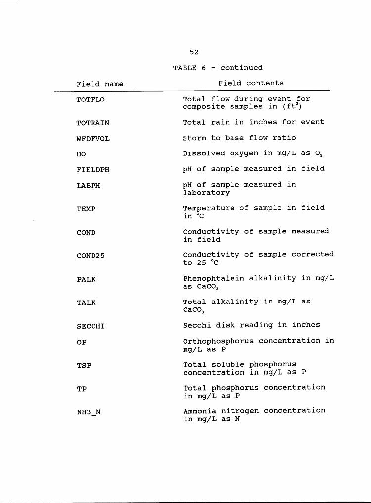
51 ITABLE 6 — Database Structure and Contents

Field name Field contents

STA Monitoring station number

LABID Laboratory ID number

DATEl Date of sample for grab samples,start of event period forcomposite samples

TIMEl Time of sample for grab samples,start time of event forcomposite samples

DATE2 Blank for grab samples, finishdate of event for compositesamples

TIME2 Blank for grab samples, finishtime of event for compositesamples

UPDATECHAR Indicates which data has beenupdated

UPDATE Date of data update or change

STRMNO Storm number for compositesamples during a storm event

SAMNO Number of samples taken tomakeup the composite sample

TYPE Grab or composite sample

DEPTH Depth of sample for lake samples

STAGE Stage of stream based on gageheight

POOLELEV Height of water in lake at thedam gage

FLO Flow rate of stream in (ffysec)

I

I

I52

TABLE 6 — continued

Field name Field contents

TOTFLO Total flow during event forcomposite samples in (ftÜ

TOTRAIN Total rain in inches for event

WFDFVOL Storm to base flow ratio

DO Dissolved oxygen in mg/L as O2

FIELDPH pH of sample measured in field

LABPH pH of sample measured inlaboratory

TEMP Temperature of sample in field_ in K2

COND Conductivity of sample measuredin field

COND25 Conductivity of sample correctedto 25 °C

PALK Phenophtalein alkalinity in mg/Las CaCO3

TALK Total alkalinity in mg/L asCaCO3

SECCHI Secchi disk reading in inches

OP Orthophosphorus concentration inmg/L as P

TSP Total soluble phosphorusconcentration in mg/L as P

TP Total phosphorus concentrationin mg/L as P

NH3_N Ammonia nitrogen concentrationin mg/L as N

T

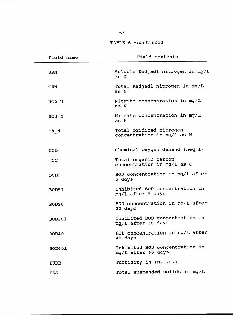
53

TABLE 6 -continued

Field name Field contents

SKN Soluble Kedjadl nitrogen in mg/Las N

TKN Total Kedjadl nitrogen in mg/Las N

NO2_N Nitrite concentration in mg/Las N

NO3_N Nitrate concentration in mg/Las N

OX_N Total oxidized nitrogenconcentration in mg/L as N

COD Chemical oxygen demand (meq/l)

TOC Total organic carbonconcentration in mg/L as C

BOD5 BOD concentration in mg/L after5 days

BOD5I Inhibited BOD concentration inmg/L after 5 days

BOD20 BOD concentration in mg/L after20 days

BOD20I Inhibited BOD concentration inmg/L after 30 days

BOD4O BOD concentration in mg/L after40 days

BOD40I Inhibited BOD concentration inmg/L after 40 days

TURB Turbidity in (n.t.u.)

TSS Total suspended solids in mg/L

I¤

54

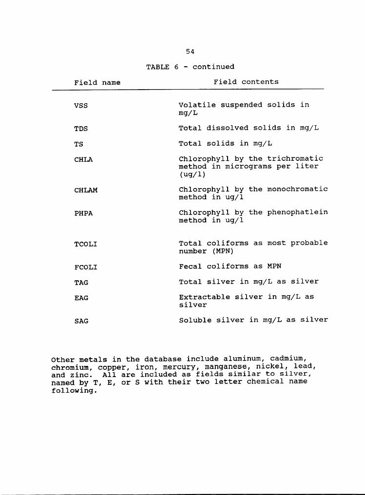
TABLE 6 - continued

Field name Field contents

VSS Volatile suspended solids inmg/L

TDS Total dissolved solids in mg/L

TS Total solids in mg/L

CHLA Chlorophyll by the trichromaticmethod in micrograms per liter(ug/1)

CHLAM Chlorophyll by the monochromaticmethod in ug/l

PHPA Chlorophyll by the phenophatleinmethod in ug/l

TCOLI Total coliforms as most probablenumber (MPN)

FCOLI Fecal coliforms as MPN

TAG Total silver in mg/L as silver

EAG Extractable silver in mg/L assilver

SAG Soluble silver in mg/L as silver

Other metals in the database include aluminum, cadmium,chromium, copper, iron, mercury, manganese, nickel, lead,and zinc. All are included as fields similar to silver,named by T, E, or S with their two letter chemical namefollowing.

Chapter IV

RESULTS

This section presents the results of the analysis

performed using the environmental database discussed in

Chapter III. Results from lake data will be presented

first, followed by results from stream data.

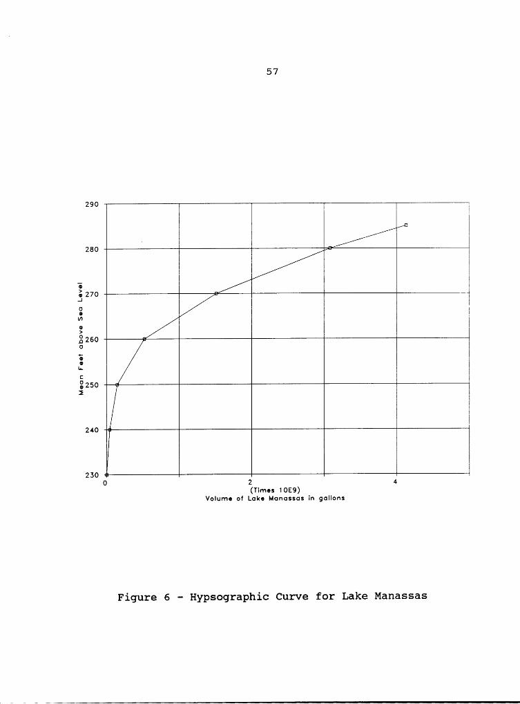
Lake Manassas Morphology

Planimetric measurements were conducted on standard 7.5

minute U.S. Geological Survey maps of the area comprising

Lake Manassas. These area measurements were combined with

elevation data to develop a hypsographic curve for Lake

Manassas (Figure 6). Table 7 gives the other morphological

characteristics measured for_the lake.

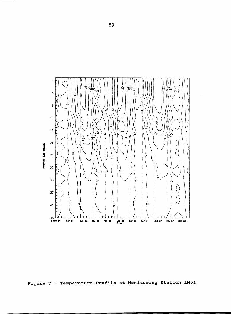
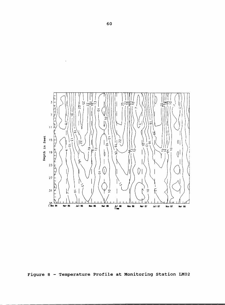
Lake Manassas Thermal Stratification

Figures 7 through 14 represent the temperature profiles

for Lake Manassas at lake monitoring stations LMO1 through

LMO8. The figures were developed by contouring the measured

temperature i11°C at a given depth (the ordinate) over the

monitoring period (the abscissa). Chapter III contains a

more detailed description of the contouring technique. The

figures are structured so that the surface of the lake is at

55

56

Table 7 - Morphological Characteristics of Lake Manassas

(at full pool of 285 feet above mean sea level)

Lake Volume 4.2 billion gallons

Lake Area 694 acres

Maximum depth 55 feet

Mean depth 11.5 feet

Length of lake 2.9 miles

Shoreline length 17.3 miles

Shoreline Development 29.5

I

* I

I

57

€ IU', I

* A I3260 LO

E0

L;.I I---2250 L

I

E H---230 ==

0 2 4(Times 1OE9)

Volume of Loke Moncssos in gollons

Figure 6 - Hypsographic Curve for Lake Manassas

II

58

the top of the graph, and the ordinate scale is denoted by

water depth in feet. The abscissa is scaled in months from

the start date of the measurements. For Figures 7 through

12, the start date was October 31, 1984. For Figures 13 and

14 the start date was August 13, 1986. The monitoring

period for Figures 13 and 14 is shorter because sampling

stations LM07 and LMO8 were added to the monitoring program

after it had been in place for some time.

As discussed in Chapter III, there may be some closed

loop contours within the figures. This is a limitation of

the computer software program used to develop the figures.

II59II

ICI I 33äöG I 32,33;; II5

cnÄ I *I I I A I I I I 19 1 — I VI I{ I I I F GI IQ I I‘° I I, 31 I I

CI G SI E N ** S Q I17 /I O O I; I II I °“

6 .2* I IQ _IpG II.; I I QI gl“* I — I I I I I I I Ic: I 0 _ O1..; QS I G I I* I I I§‘29 I I I I I I Ö 4I I; I II I2 I I I3

33 O O. I IN I I I I I IG I37 I I I I I I I I OI

I I _I I · I I I I I Q"‘ IQ I I QI I I* I I I45 . I 1 ÄLl|I¤v84 Mar 85 Jul 85 ||0v85 N|r86 älnßö ||0v86 Mar 87 JuI87 Nov 87 Har88

Figure 7 — Temperature Profile at Monitoring Station LMO1

60 Z

3 I I I ämgfvän I IIII I I °IIC I I I I

H I I I ~I 3 I IC I I 9 I __ I II I Igw I; I} I IEM QSI IEC}! I III

I I I EIBIZE OlC I I I I

P I I EQ) I I I?I I (I33 I I, I I I3* I„ }! I 9 I I 9 I3

—' · I 4

Figure 8 — Temperature Profile at Monitoring Station LMO2

I

61 II

II I I TFIIBLQS I I I SIIQIU

4 I II 6 I 9;,; I IS I I

8U”‘E II I I II I I II; 4 I

812 I III I I I I I ag I IC) I

Ü; UI m Ig;3 I

I .4 LI 4INOv84 Mar 85 JuI85 IIov85 Iurßß I•ov86 Nur 87 JuI87 Nov 87 Marga

Figure 9 - Temperature Profile at Monitoring Station LMO3

62

7 I I MI77 I3 I IIII7[Q2 7 I lg I I .

ä I ml’ I I II I 7 IQ I7 S

IEISÖI 7 I SI I <I II I I’° gl I I I Iäg ‘° “° II7I (I77 I I I I I I (I II gl I E l „l¢‘—” I I3; „ 1 4 I

Figure 10 — Temperature Profile at Monitoring Station LM04

I

I63

I 1 1 1 1 12C:I _ 66;. Ö mag, "’6„3”¤2§»6 » IÖ

@6 In ;„ I · I I Q5 1 61 1 QI ow ·> NUII

ä8 I I I I I ‘ „I 2 I5 I 5’ 1 5 5 1 @1 ~I5 °“ “ 666 „„_E (Ä) EF)0 Em ä dl QGQ wal <)I 418 Q O@2 aI ® GI IO G ·22 I I ’° I5 I I I

_ „¤I IJ I I 5 I ;,,I 455 1 1 1~» 1 6 1 1 1 ~» 61 1.. ,. ·— 0;-/

jpNov 84 Mar 85 Jul 85 Nov 85 Mar 86 Nov 86 Mar 87 Jul 87 Nov 87 Mar; 88

Figure 11 — Temperature Profile at Monitoring Station LMO5

64

KQ Q I I_ I8 I _/ I I Ig 3 , ägmß. Ä} «¤ > "*04Q n I I O I N I I"" V 70 N EQ 7 Q I I IQ 21 I8 r

Q I3 I O I I I <H’

Q /0

E Q I6 Ip es QI Io \„I5 Ä

‘Kn 1 I L 4K1

nov an nov as Jul 85 nov 85 nor 86 QQL86 nov 86 nov 87 Jul 87 nov 87 M, 88

Figure 12 — Temperature Profile at Monitoring Station LMO6

65

LArx

wG"" .4:2 .·-•

,,— 4 5 °° ·'?>° äj 9*56 „ EQ 6 6 ‘* ”P » :,4 2 626 9 ”‘

Gi? 6/0 KÜ"/

40“O

YZ • $4 ‘Unna Umcu U^P'°‘7 H- UMUB7 l3D•c87 l3Apr88

Figure 13 — Temperature Profile at Monitoring Station LM07

66

J J G2 I

G6)I

I I I I ® 6ET Q 2Z I I I I* Ggs I I I (P .

I ’\

NI I 07 U"

s_ Q AIQQIIQQQQ “°°°“ IMP"? nu l3A¤¤87 1:061:2 13 I Q

Figure 14 - Temperature Profile at Monitoring Station LMO8

u

67

Lake Manassas Dissolved Oxygen Profiles

Figures 15 through 22 represent the dissolved oxygen

profiles for Lake Manassas at lake monitoring stations LM01

through LM08. The figures are developed by contouring the

measured dissolved oxygen concentration (in mg/L) at a given

depth over the monitoring period. The figures are

structured so that the surface of the lake is at the top of

the graph, and the ordinate scale is denoted by water depth

in feet. The abscissa is scaled in months after the start

date of the measurements, as in Figures 7 through 14.

Figures 23 through 30 represent the percent saturation .

of dissolved oxygen for Lake Manassas at lake monitoring

stations LM01 through LM08. These graphs are a combination

of the temperature profile graphs and the dissolved oxygen

profiles. The percent oxygen saturation corresponding to

each dissolved oxygen measurement was calculated based on

the measured temperature at that location. These graphs are

structured the same as Figures 15 through 22.

Note that for these figures closed loop contours are

both possible and expected because of the presence of

submerged microorganisms (algae) producing oxygen by

photosynthesis.

9

6gf °‘

Ci

W,

OQ;37

T.„

LI

ÜII/III1I//Aix O

gw J )\§/ OO L/66 L IE IZIIQIQI·III QQ31

“V‘IL“VI°Figure16 - Dissolved Oxygen Profile at Station LMO2

I

70

0 I I4 9 °O E oo °°O

vu //8 8 I Q 0)/IIll(O co-•-{ <O

I6 g' \ /0/\ 88 \\ }¤°° 5 2 ram O

. /\ _I „ IIIZIONVN wlhrö JH85 I0v85

A·hvö lhr87 JAI87 hv87 hrs!

Figure 17 - Dissolved Oxygen Profile at Station LM03

j/1/W1Ä

III

72

N Ä I I > IX I I I III IIP4I I ’ — I I ‘I. II I I I I*’ ,/I I O I II I

LI I I I 8/I I I (I / Ä F/I I I17 I

IIII I II I I FS I/I 0

,' . I1__¤•

II II I ;C, I III°° II IG I I I OV I

I /0 / \‘X22* 8, kJ I II/cI I II 6=

2O VLOII,/I II

/I /I85 88I

88Figure19 - Dissolved Oxygen Profile at Station LM05

73

IIUI

x\I""

/7 Ix „ ß \ I I5 // III IQ4 ‘ ‘ ’ / I gI1 G? xx (O OG //

R 5/ ~Xy \_‘I7„X „ I 7/ IX \/ \/F}‘\.

'’

"I I I}§>xf~8ÄW¥ m•·2?s—'° u¤v6s‘“'°°nTWi"§l?6‘i "i•6§66‘¤§·’67 adi 87*--Tov 87 niä

Figure 20 - Dissolved Oxygen Profile at Station LMO6

I

74

I I I ^ I 3 I I ·I

I I ‘ E °° ·I @*H ·\I I I F¤ XX I @3 I I I *3 / I·•-I 4

I \\u ‘— I S' \) io _ /7 I3 c¤ OI I II \ • I I I I '„ II rl /I I‘i;W§?•€—’ II *i$‘¤¢T662"‘* ia ^TIIW"““F¤ä’——‘—ü@—*—‘

Figure 21 - Dissolved Oxygen Profile at Station LM07

11

7 5

O1

1 1 1 1 1 1 Q 12 6 1 1/‘1 9 \ 1 111

Q 1 1 OO 1 1 1U 6 6 1 ; 1 1 1 1 L1 ÄQ 1 1 / 1 1

1 1/‘*·‘

1 rx \11 V 1 1 1 1 1 Q-/1161., „' 1 1 1/„¤

1 1 1/ „ 1 1 1 Q8, 1 1 1 1 1 /— 7G! Ä 1Q 1 ¤¤ 2 1 2 1 1 11 / 1 °°J1’1 1/ 1 1 1 «’1 1^\ 11 1 1 1U 1

13 MTU 13 Dec 86 13Apr 87T1

13Aug 87 1 13 Dec 87 Apr 88Z

Figure 22 - Dissolved Oxygen Profile at Station LM08

Ä . ~ Ä igix j Ä O9 *9 ÖO 99 M ./OÄÄ Ä

99 Ä 99 QSÄ Ü Ä4“9Ä..®ÄjÄ?Ä(.lÄ]<@>Ä ..< Ä„... .. .. . 9..]* ..>.

3323

E3O

A

Q3 \\)€‘£%䧩(\i% ip‘ i ( NM xi Q/AMB ij J

Figure 25 - % Saturation DO Profile at Station LMO3

3; *66M¤«@

6A6 Qw 6 /~ 6 @$666 <®g}@6&?¥if6$“4?’6‘§?6?6

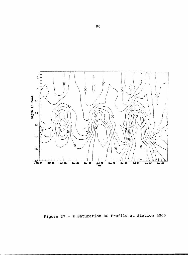
2 OVX]

of N VO » K

<'Figure27 - % Saturation DO Profile at Station LM05

81

u 3 //,’ /·=/'\

2 7 \_/ U( O /1

‘*~·@ ¤ 7@ F 3 Q, g1 •• mas mas mas ••••-aa #26 man mar mar ama: man

Figure 28 - % Saturation DO Profile at Station LMO6

82

·* U 2 / 7 ~ in 7Ä \ 6 6 Ä ) an

. ~ /g ,7 "

7 ‘\

>A4 \ /U / j

E n ‘ \ O? <>“7M)8

-l[._.n..4..l..na£n.- .names nn¤•¤a6 neuw “_ne~·¤w num; „„„„

Figure 29 — % Saturation DO Profile at Station LM07

i

83

·"—’*—Y"T“Ä—°"fgf

3 Üg lg *\}<;>\\°••

){C}tg

lyß2/l/ 2

\\un.;umen 13l•r87 H- llmßl 130•c87 xappaa

Figure 30 · % Saturation DO Profile at Station LMO8

I

II

84

A different presentation technique for the dissolved oxygen

data was use in Figures 31 through 34. Figure 31 is the

dissolved oxygen data for monitoring station LMO1 plotted

against time. Two curves are plotted, one curve

representing top waters for samples taken at the one foot

depth, and the other curve for bottom waters representing

the samples taken at the lake bottom for that monitoring

station. These plots are called bottom and top plots.

Figure 33 is the same as Figure 31 except that the percent

saturation dissolved oxygen data are plotted.U

Figures 33 and 34 are the same as Figures 31 and 32

except that the data for monitoring station LMO8 are used.

It should be noted that the LMO1 figures represent

approximately four years of environmental monitoring data,

whereas the LMO8 figures represent approximately two years

of environmental monitoring data. Additionally, some of the1

top and bottom plots indicate that values have approaching

zero. The author considers it important to stress those

data points that were measured at less than the detection

limit for that parameter. By graphing these data points as-

as half their detectable limit, the data is emphasized.

Furthermore, it helps overcome some of the scaling problems

associated with graphing data that extends over orders of

magnitude.

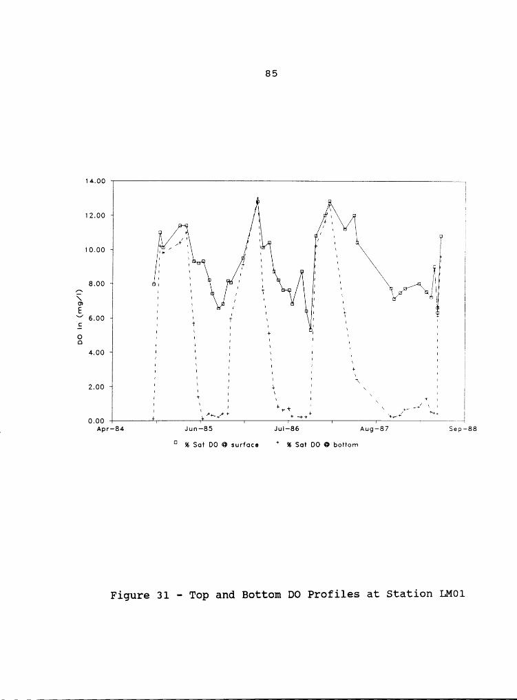
I

1II

8514.00 II1

12.00 IIII„„ I I I

Äu /+/ II II H [ II uT10.00II_ / I II I I I Iu I

I II „ za II I I IIII I I nv n IIII u EI. I I n I I

I| I I II I II I I- ·I .. = = " ·

I I III I I é I

I I M I u I I

é I I B II I u I I_I I "' IS · 1 T Y Y I Y IO I I ' I I I ‘

O I I I I I I II I4.00 · · I I I ‘I ,

I I I 1 I I I II II I I

III ‘I'I

II I I I I +\ I2.00 I I 1 · X I

\ I II II I I I \

\ * II I

**+~+/*" + 4+ 4 +’ "** I0.00 " eiI Apr-84 Jun—85 JuI—86 Aug—87 Sep—88

Ü SIS Sat DO Q surface I % Sat DO Q bottom

Figure 31 — Top and Bottom DO Profiles at Station LM01

86

160.0011140.00 " 411

120.00 .1 {O

hull V4

R" JO 100.00 ¤ ,_ ~1 6 4 Qc " „ r 1* ‘ ° "rg 1. 'J 1 J1 1 J1 T

E 4_ ,·t{ Ä\

n E/ 1 J

2 80.00 Q1- Q /4; 4 ·· I 1 Q1I0 1 J

1,1 J ‘1 Q1 1 ·· ; 14 ·& 6000 Ä J ’ 1 '

‘ '' QJ4 T 4 1T·1 I ‘ Ä

‘. E 1J J I

+ 1 1 1 1

40.00 Q‘4 1 Ä 1 1 1

l 4 l \ I1 1 Ä ‘ Ä 1 Ä ,1 1

‘ 12000 1 1 Q 4 Q

‘\Q 1

J 1 J 1 „1 J ‘ 1 1. JJ

11-0001 “Apr—84 Jun—85 Ju|—86 Aug—87 Sep—88

D % Sat DO @ surface + % Sat DO 0 bottom

Figure 32 · Top and Bottom % Saturation DO Profiles

at Station LM0l

1II

87

14.0011

II I1 I~ ¤ \ I+ I

12.00 , ~__ I

/ \\

I+ I

I1 n /¢ I1 \ / II

_I \\

+ I1 ‘ 1 I ”IIII I I „ \ I If

10.00 . ~ I 1 In II ‘ I I ‘ / I II u I ¥ \c( 1I

II I

e 1 1 I, 'I.tnI \ II 1 ~

II II ; IE 8.00 I I I + I,xy

I + I 'I I Eu u I I+ \ “

II + u III I II I 1 I3 1 " I ‘ I II 1 1 1 ' 1 I

6.00 I II . , I I1 II /I 1 I I \III I 1 1 I I'4 I I \ I

I I 1 II1' I I

I1 1 I I4.00 II I I

I1 xlI 1I1

2.00M¤r—86 Oct—86 M¤y—87 Nov—87 Jun—88

EI DO ct Top I DO ot bottom

Figure 33 - Top and Bottom DO Profiles at Station LMO8

II

88

140.00III

120.00 Q+~

_ +IIEI

III III Ia I I010000 Ä IQ \ I III II /\ \ I; I I I gg IE I Q I I I T T3 \ / I I \ 1 I I I I I'°ö II I I T I I I I I IVI 80.00 I I I'

‘I ,‘ ‘I I II I' IR 0 I ’ I 1 I, III + II I \ / I I I

/I I \ / I I I II I \ / I I I;II II 4- I I 4 I

I

6000 ß Q · II · .' I

I II I

*II

X-40.00“¤'·86 O¤t—86 M¤y—87 ~¤v—67 Jun-66

G SIS Sot. DO ct top + % Sot. DO ot bottom

Figure 34 - Top and Bottom % Saturation DO Profiles

at Station LMO8

I

89

Chlorophyll a Profiles

Figures 35 through 42 are plots of the Chlorophyll Q

concentration at the lake monitoring stations. Contours

with depth of Chlorophyll Q are not possible because this

parameter is not measured at depths other than the surface

(one foot depth).

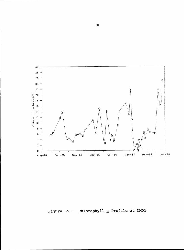
I

II

90 II

30 II2826I[PI24 I I1 I

22 II 1““ I I¤I1 IuE16o „ I

i 14 n II Yl.c u IS12 „ ,E n u IE 10ll9 „ ·· I I8 I” I6 'J “ ==!¤ u ” J®fB\$ II,¤ u 1

4 B “ uu H u nn

0 2 2Aug—84 Feb-85 Sep—85 Mor—86 Oc1—86 Moy—87 Nov—87 Jun—88

Figure 35 - Chlorophyll Q Profile at LMO1

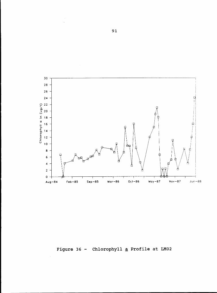
. I

91

30 I28I26 I2422 II

II I IS”20 IIV u IE 18 u 1 I¤ I IZ 16 ¤ tp;

E n uIQ_14IEI 19 12 v•ib‘ :° 10 n H1 18 ” E S . · u III I

'I Il

6 u rs ZZ I ZZ U uI„ , J u

4 E J n u “ n VII1 1 KK I

() 2 = 2 ::

Aug-84 Feb—85 Sep-85 Mor-86 Oct-86 Moy—87 Nov—87 Jur1—88

Figure 36 - Chlorophyll Q Profile at LM02

92

3028 12624

22g,20 \ 13 1. E18¤16

: II 1Q 14 n I¤.S 12 Ié 10 10 rs“

u “ ,E || II

8 Q; 1H B16¤‘ u H ¤¤ ¤ ' 1

ra W ‘¤ ”‘=¤_ „4 n

“1“ ..2 LJ

Q FJ 2 2 IAug——84 Feb-85 Sep—85 M¤r—86 Oc1—86 Moy—87 Nov-87 Jun—88

Figure 37 - Chlorophyll Q Profile at LM03

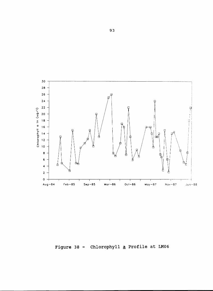
93

30 I2826n I

H24 n I,3 22 II $1g, 113/ 20II2

*8 il11 "1_16 u v: :• II;_ II IIIä14 u I In u u I IE 12 ·· \ I IE u u IU 10 n“ u

XR1" I

8 1[lu u M I

4“ Ü

Ü:.6 ” 6111 I

SI2„Aug—84Feb—85 Sep-85 Mor—86 Oc1—86 Moy—87 Nov—87 Jun—88

Figure 38 - Chlorophyll Q Profile at LMO6

94

so

28262422

In 1.6 18 I“ I.2 I IO 16 ¤=• /2,4% I

i 14 n n Iä

‘ E0 12 an I5 „ „ ILE) 108

„ ‘ II6 “ I

41I:IZI

I I2 III

0 22Aug—84Feb•85 Sep-85 Mor—86 Oc1—86 Moy-87 Nov—87 Jun—88

Figure 39 - Chlorophyll Q Profile at LMO7

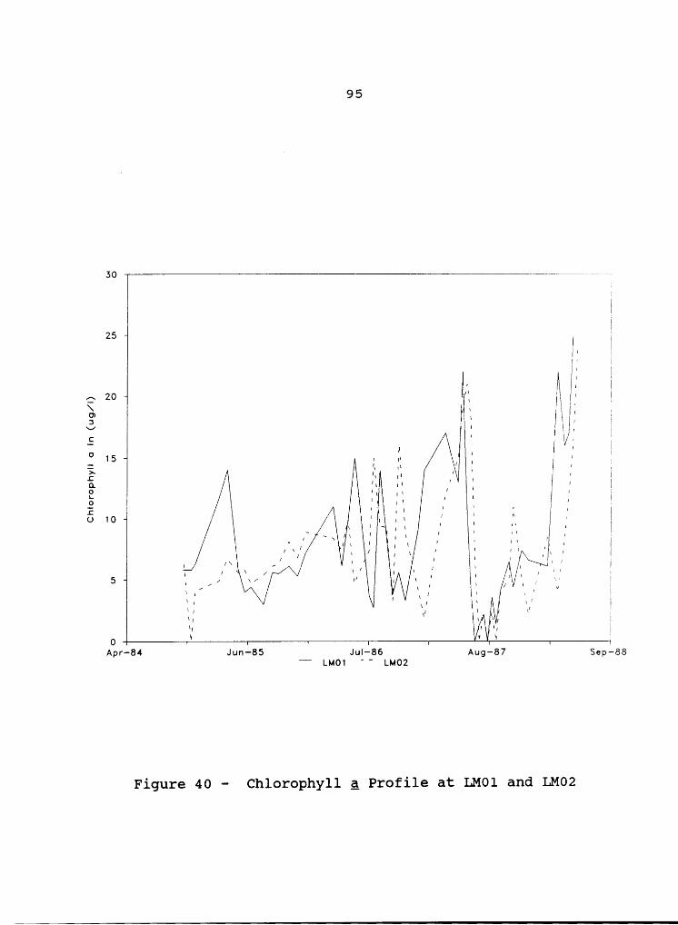
I

I

95

30 „-IQI

III25IIIII II I

| IIIQ

20 III I II ‘ II I3 IIIcI I I

E I I I I15 I II

I I I

: I I I 1I Il I

E II II II Q I III3 I: :2 I I J !

Q I II I I I

10 I I I I I I II I II I — I I I I II I II I \ I// \I/ I I] I II \ /I\II

/\ I I \III \ / I I I I I I I I II Q

5 I II I I I I I I I III I I I I II II I I I I I I III] I \/ I I] I

I I I FII

III

III II

II I0 I ‘

Apr-84 Jun—85 JuI—86 Aug-87 Sep—88— LM01 ° ' LM02

Figure 40 - Chlorophyll Q Profile at LM01 and LM02

96

301

1ie 425 ’ „ 1

I „

I I Ii ;I u ' >ll I ä‘: u'

20 l I I l‘ ;‘ 1/\ \ 1 \ I \ I

( Q ,Qg°'Ä ,’

··‘ Ü ·f u \•‘

' I {I \ 1 I I Il „

• 1 E u \: I I- — In '

{\ I

Ö l‘\/I

\ : Ä II

V \ IE: ^lä

|I‘ /\ llU I I I

Ijl I

,ln I \ I

%x , I s zw 1

Ä‘ "„ /,~'

: 1* ‘ ’ "\' :‘ :\\· 1OwL

In ‘1 \' *

\ I x' I ‘1 ä

O'

• ‘J I In I m' ¤ *

I\—¤ z «

6 10 ,l‘:

’ 'I l" I ‘ I : I, I‘I x ' I

"‘ I a ‘ ‘ \ ° i

l‘ E \ / \ I

‘ \ I }

' „· ' . ‘

· ·{\ I l \' \ I 1

5ll ‘ I ‘« IV x '\ I \| ‘|4«

, «!\„ ,· „INI I 3 i

O iApr—-84 Jun—85 Ju|—86 Aug—87 Sep—88— LMO3 “ ’ LMO6

Figure 41 - Chlercphyll g Profile at LMO3 and LM06

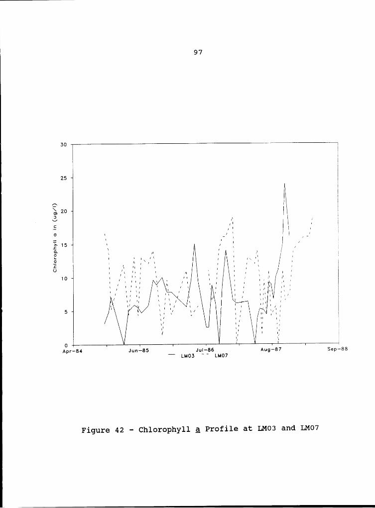
97

30 I

I25 IIIIQ 20 I

II I1C/I 1 IO I I I: I

,_I I /“I>~

15 I I II I 1IEI Ä I I

I I / I 1 E

I II :\ / III I Il\

J I I I

I II II I I I I I II III II I I II ‘ II I II I I I I

1O I I II II II I II I I I II I I I I I II II I II I I I I I II I' II I I I 1 I II I

III II1 I I I I I I I 1 I II I

1 II I I I III I I I II I

II III

I III II I I I II I I I I

5II I I II I I II I

II I1 I IIZI III II}I

O IApr—84 Jun—85 Ju|—86 Aug—87 Sep—88

LMO3 " ° LM07

Figure 42 — Chlorophyll g Profile at LMO3 amd LM07

98

Figures 43, 44, and 45 are additional comparative plots

of chlorophyll a concentration at different locations in the

lake. On Figure 45, the data for station LMO7 do not span

the entire range of the abscissa

I

|

II

99

Z5

II 1IIIIII

1 II20 I II II II 1I I

\ 1 IEI ' 1I 1~/15 I , IE 1, 1 I¤• „I· ,'I

II II II IIO- 1 I I I 1 I9 I I 1 I 1 I

9 10 1 I I I I I 1.C 1 , I 1 I I I IO I\ I 1 I 1 I I 1I I I II I III II

_ I II I I II I \ I I II I I I II II I I I I II I I ß I II

I I \1 III I I " ” I II

/ I \ I_5 II \I I II ~ I I I \Il

[ I I I I \ I[ I I I II \ I

I I II II I 1I I II \ I\ I II IIII II IIII I II

OApr—84 Jun—85 JuI—·86 Aug—87 Sep—88_°

LMOI ° ° LMO}

Figure 43 - Chlorophyll Q Profile at LMO1 and LM03

100 I

30

/

25 1{I I

I I 1 II1 I I

1 I I I II Iew I 1 { {Y I;I‘ 'I Y II II

E II I III 1IV .1 1 , J1 .1

IEIII Il

II\‘ II

"II

1 I 13IS 1 ^'I1I I II I'I ‘I; II I 1; I 1 I I I I II1

' IIAI

C 11 I I I I I I II 11 IS- I I I I; I I I I I III I II I

II / \I I I I I I I I II I

\I

- 1 I 1 II I I I 1 1 IIC I I 4 I \

O IO II I 1/ I ’ I I I I II { ‘III I 1 I I 1 I I I

I I 1 I I I II I I II 1 I 1 II ' 1 II 1 I I II 1 I 1 I1 ' II I IY . I 1 '1 ·T 15 I I 1 I In

x I 1:\I II

Q AApr-84 Jun-85 JuI—86 Aug—87 Sep——88— LM01 ' ' LMO6

Figure 44 — Chlorophyll a Profile at LM0l and LMO6

I

101

30

25

20E .\/ I1E llo I "_ \ _I1

· /:15 *1 ’ 111 I I01. 1 1 * 12 ~

,‘1 1 1

I I1 I\ I I

O'

II I 1 1 I*I«<> 1 · fl J J 1 1 JII

' * 1 * ' II 1 * 11* * 1

*“II 1 ' 1Il

* 1 ***11 11 I1' * 1 *,*11 1 1II *1 *::11 1 ~

I I I5 1 1’ ;;1 Z, I1* 1:\‘

1 II III II

O‘

Apr—84 Jun-85 JuI—86 Aug——87 Sep—88_LM06 '°' LM07

Figure 45 - Chlorophyll Q Profile at LMO1 and LMO7

1

102

Lake Manassas Nitrogen and Phosphorus

Figures 46, 47, and 48 are plots of ammonia and

oxidized nitrogen in the bottom waters at LM01, LM06, and

LM07.

Figure 49 is a plot of the oxidized nitrogen in the top

and bottom waters at LM01.

I

II

103

2.5II

IIII2 IZ I"' I° 2/'\

},, 1.5 I\./

Ec2E Ibc 1 I¤ Ic I° I° I

x I1 I\

’ \ 1‘ IO‘5

/’\ A I J \ I \ 1 \ I[ \ /\ \ [ \ I \

[ ~ I I \ , \ 1 x

/ I , \ / \ /\ 1 1

//

" "

\\ //\\ /

O \ I ~ /Oc+—84 JuI—85 Apr—86 Nov—86 Jun-87 061-87 M¤y—88

” NH3_N of boffom ' ' OX_N ci boffom

Figure 46 - Nitrogen in the Bottom Waters at LM01

I

104

2.5

I2 IZ IM I0 IQ I\ ICD 1E1.5g

I* Ic I_g It“ Ic¤ 1U IC .o0 ,I _ I!‘ [I 11 II ~ / II11\ I ‘I I, II I1 1I I

1 1 I I , I 1 ‘« IO.5 I I 1 I I , I I I1 1 / I , I ^ 1 1 II I I! \ I \ ,,I\\ I 1 1 ,1.I!\\ I/I II I Il I I III

\ \I \ 1 1 / II 1 \ I 1 , /. I

0ct—84 Ju|—85 M¤r—86 Sep-86 M¤y—87 Sep-87 Apr—88— NH3..N ot bottom ' ' 0X-N ot bottom

Figure 47 — Nitrogen in the Bottom Waters at LM06

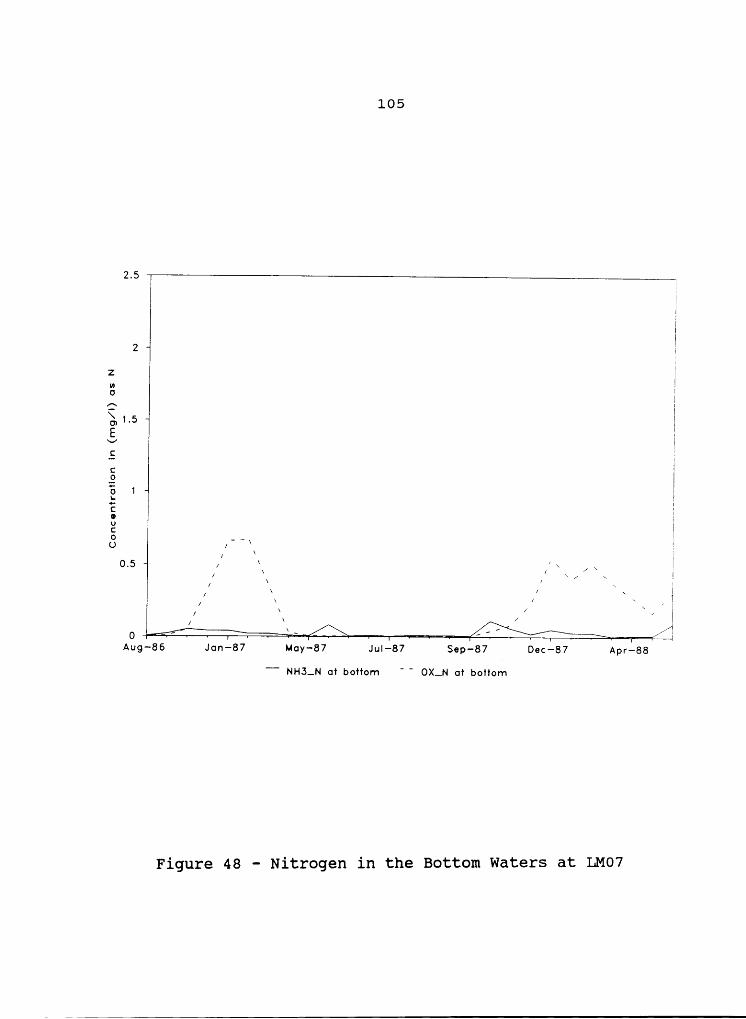
I

II

105

2.5 4IIIII2I

Z I3 I3,1.5 IÄ IE IE I6 1 Ij; I¤ I° 2U Ig IU 1- ·I40.61 *4 ,’ \„1, 1 * / \ I/

\ /Ä\1

4 4 I1 ’ I1 IO ‘ W , W W .. W I

Aug-86 Jon—87 M¤y—87 Jul-87 $6p—87 Dec—87 Apr—88““ NH3-N ot bottom ' “ OXWN ot bottom

Figure 48 — Nitrogen in the Bottom Waters at LMO7

1

106

2.5 ,1 1

12 1Z 1w 1Q 1

°’1E 1.5V 1E 1S 1·;: 1E 1E 12: ‘ 1c 18 1

x 1 1x \ 1

0.5 A I \\ /\ 1 \ \\ / \ I \ \

// \\ I1 \‘ \\/ \ l \ " ^\ \ —\‘ ‘ \

061*-84 Jul-85 Apr—86 Nov-86 Jun—87 06t-87 Moy—88—' 0X-N ct Top ' ' 0X_.N ot bottom

Figure 49 - Oxidized Nitrogen at the Top and Bottom at LM01

uu

107 IFigures 50 and 51 are plots of the total nitrogen and

total phosphorus in bottom waters at LMOl and LM06.

Figures 52 and 53 are plots of the phosphorus

concentrations in the bottom waters at LM01 and LM06.

Figure 54 is the plot of total phosphorus in the

surface waters at three monitoring stations, LM01, LM03, and

LM06.

I

108

3 II I

2.5 I I

S I IU1(IE I2:1.52*6

I,2 I¤ I02 , I6 II II I I\

I/I I~\ /I I

Q_5l\II

x_‘

A// \

\

OOcI*—84 Jul-85 Apr—86 Nov—86 Jun—87 0cI—87 ”McIy—88— TKN cf Boffom ’ ' To+¤| P of Boffom

Figure 50 — Nitrcgen and Phosphcrus at the Bettom of LMO1

I

II

109

3 II

2.5 II

2 IE IE IV IE I.5 Ic I2 IB It I¤ IÜ Ic I I<> IU II

0.5{/^\

/ — r-Il \\

\ A /O ————·' ‘——-··^~ ‘ *-9 x’\»~--—~__ , ’ r —1 ~»\tOct—84 Ju|—85 Mcr—86 Sep—86 M¤y—87 Sep—87 Apr—88

V V TP ct Bottom ’ TKN ot Bottom

Figure 51 — Nitrogen and Phosphorus in the Bottom at LM06

l

1

O.3 I I1‘I 1 I 1

1 ' I 1 1 11 ‘

I 1 1 11 ‘

1 1 1‘ 11 ‘1 1 1//1 1 ‘

I 1 1 10.25 I I 1 1 I I 1 II II 1 1 ' I 1 ' ..111 ‘ 1 ' II 1I I l I 1I 1 1 I 1 1 1 1 I1 I II \1

1 ‘|

I , 1' 1: I I'I1V I

I 10*2 I I 1 ·I \I 1 I1 1I I11‘ I ‘· I1 I 1\ ,1 ‘ °

EI 1 l 'I\I I I \ I11I

1 1 ’ I‘I 1 I 1 1I I 1 I1 ‘ I I 1\

' 1 ° I1 ·‘

I I 1 ' 'I1 I 1*I I 1

0.15 1 11I1 1I l ' 1 I 1\I I 1

I I1 I 1I 1 1 1 I '11* I 1 I1 1 I 1l I

1 IIl

1 1 1 1 1 1 ’ 1 . 1 11 I I 1I I I 1. I I1 1 ‘ 1 1. 'I I 1 1 1 ' 1 I . '1 I

1 1 ' 11I ‘0.1 I\ I 1 I I

I1 I 1,I I I I1 11 ‘

' ' · 1 1 · 1 ’· -—11 · ' 1 " 1·1 1‘

1 1 · I‘

I 1 '1 ‘ I .I '1 , 1 1 1 , 1 1, — I 1 — 1I I I

‘1 4 I

_' I 1 II I' 1 1 I\ 1 I 1

‘/ I

'I\l0.05 I

III 1 1 1 I 1 I.‘ ‘1 11 1 I

I II · 1 1 ' I 1 I I ' .' ‘1 1 1 1 I!I II 1 1 1 ' I 1 , I I ° .' ‘1 1 1 1 I

I \ / I 1I I- — d / I I 1/ I I I I1 I1 1 \ 1 1 II \1 +1*- II 1 ' 1 . \ /‘_ 1 „ ‘

I 1 ·, _, ‘ ’ X VO

Oct-84 Ju|—85 Apr—86 ‘ *Nov—86 Jun—87 Oct—87 Moy—88

Ortho P ct Bottom TSP ot Bottom “ TP ct Bottom

F1gure 52 - Phosphorus lh the Bottom at LMOl

I

Illl

O.1 I1I I 1 I· · 1 1 ;I I II III1 II I 1 II ' II 1 I I1 II1 I I II II1 I 10.08 1 1 ' I' 1 I 1

1I 1 I II I I II1 , 1 II 1 I 11 1I1 1 I II I I IIIII 1 I 1 I 1 II I

I 1 IIII II I

II I\ I I II II I I |‘

II II II

IO, [I I I I IIII II I I I I IIII1 \ 1 I I 1 1 111 I1 II 1 1 I1 I11I1II I1 I1 I II. I I1 I1 1 1E ,I I11 II 1 I [I1 1 11I II 1 I jI I 1II I1 i

C I I 1 I I 1 I II III 1 I I 1I 1 I1 I I II II II1 1·

I ,I1 1 I 1 1 I I 1I 1 1 11 II 1 1 I I*6 I 1 I 1 1 1 1 I I 1 I 1I 1 1 1’ I I Ix-

Il 1 II 1I I | I II II I I 1 I*_ I 1 I I I 1 I 1 I 1 I 1 I1 I I ,

E 1 I I 1 I 1 I 1 I 1 I I I II 1 I¤>¤-O4 ' ···· 11 1I / I 1 1 1 I I 1C 1 1 1 I 1 1II II II I I I II III I1

I II III

III-1 1I I1 ·1I 11 I I I1 I I II 1 1 I1 I1I I 1 1I 1 1 1 I I —1 11

I1 1 1 I II \ 1 II I0 O2 I I I I I 11 I I 1 I I·

I ' 1 I 1 1 ‘ I;II 1 1 1 1 III I 1 1 1 1 I

1 IIII \L T1 IIIIII I

Q 1Oct—84 Ju|—85 M¤r—86 Sep-86 M¤y—87 Sep—87 Apr—88

' ' OrthoP ot Bottom — TSP ot Bottom ' TP ct Bottom

Figure 53 - Phosphorus in the Bottom at LM06

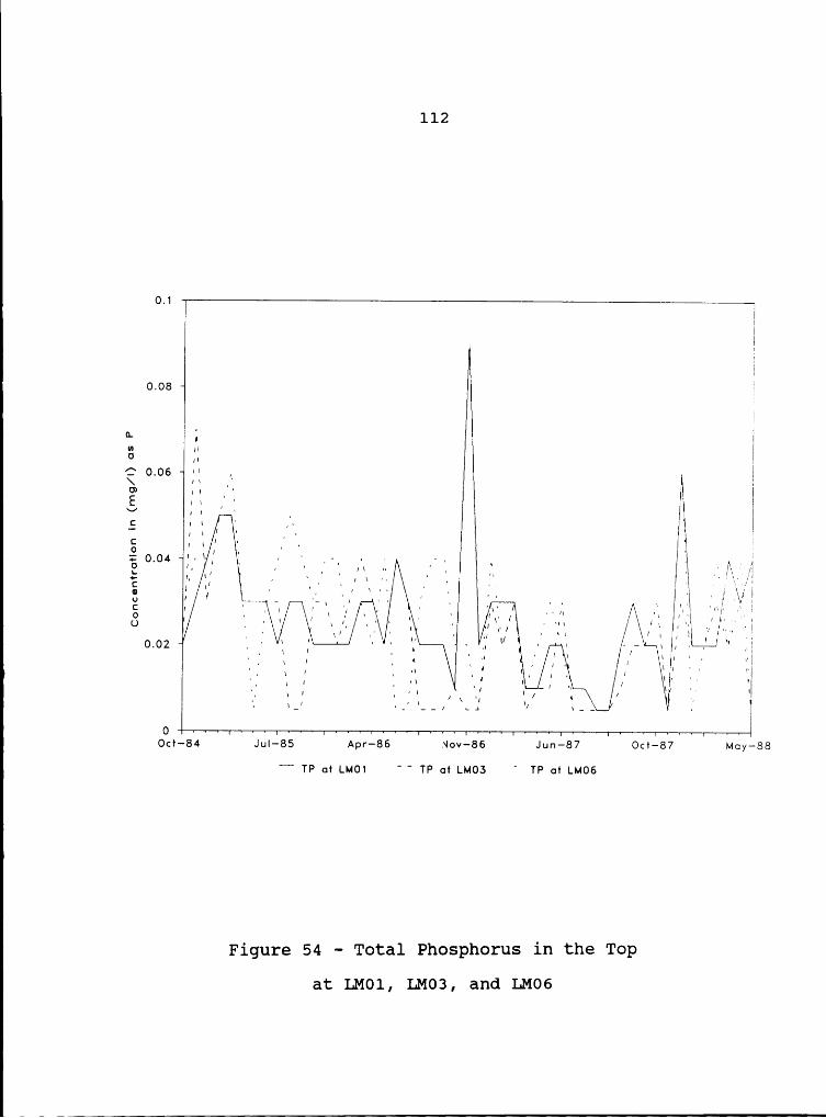
I

II

112

O.1

ä1

0.081

¤.*6" }n Tc 0.06 ·· , i\ M ,' 1U) • 1 ‘ '

E I Y I‘

\/ I \ T IC 1 \ ‘

I „Ic I · TO { \ 1 „ ' ‘

f i%0.04 :·‘, ‘ · ‘ · - _.tIll \' lv ‘ ll \\ VM. I I II {"‘E¤ ·#’ I w —·— I Ä " ‘L T; x

IIII jr _ ~_ ‘ , . · ' · ‘ — . ' TE ' ' ~ ‘'

\\ Ü,· ' l. "‘ Il, «\ [Ü '/"{

"j

I \"i'T\ / 1 /¤» T

002 . ' { T', N ‘M · ,, V · ^¤ / • ,T.

,\ 'I · I ‘ L1 V'

‘ /· \\ V,1*

° .I \x' "

\, J ‘ ,’ ,I ‘. [ I I ‘"Il I I I

•\ ‘ J \ _} W /‘\' \" Y‘«

\ I 4 I I /‘/ I / ‘ / [ ‘!

‘, \_1 _—· \‘-J' \/ ‘ ”'1

OOCT"84 JuI—85 Apr—86 >Iov—86 Jun—87 Ocf—87 May-88

—' TP ct LMO1 ' ' TP cf LMO3 ' TP of LMO6

Figure 54 - Total Phospherus in the Tcp

at LMO1, LMO3, and LMO6

113 ILake Manassas Watershed Properties

Table 8 gives the data for the five basins used for

this thesis. Figures 1 and 5 show the relative location of

the basins.

Figure 55 is a plot of rainfall in the Lake Manassas

watershed on a yearly basis.

Figure 56 is a plot of the Percent of Runoff for the

ST7O basin as a function of rainfall. In Figure 56, the

points represent actual data and the straight line is a

regression fit of that data.

I

114

Table 8 - Properties of Lake Manassas Watershed BasinsBasin Area Percent of

Tributary Name (sg. miles) Total Area

BR03 - South Run 7.47 10.2

BRO4 - North Fork 8.32 11.4

BRO5 - Northern Arms 3.11 4.3

BR06 - Southern Arms 2.67 3.6

ST7O - Broad Run 40.43 70.5

115

w*Q " u

„ 40 V \‘IIIIIIIIIlll' -.C S _

.E „ , ¤

Z so ‘

'ö(Z 20—

Xo

W—1974 1975 1976 1977 1978 1979 1980 1981 1982 1983 1984 1985 1986 1987

Year

Figure 55 - Rainfall in Lake Manassas watershed

l

ll6

50 ($lrcighl line ls c regression fil)/

45 "/ ܤ //

L. 40 /OC3M

3; 35_ E

Ou0)

f 50O.C: ¤E 25EUM ¤“6B? 20 D

15

1O

lnches of Roinfoll in a year

Figure 56 — % Runoff into Broad Run versus Yearly Rainfall

117

Lake Manassas Watershed Environmental Monitoring Data

Table 9 is a summary of the database for the sampling

of the drainages into Lake Manassas. The table contains the

maximum, minimum, average, median, and the standard

deviation values for the listed parameters. For sampling

station ST70 a flow weighted average value is also listed

because flow data existed for this station. When the

database was analyzed, if a given constituent was less than

its detectable limit, it was evaluated at half the value of

the detectable limit. This way a parameter value of zero

was not "averaged into" the analysis. In most cases, if

this was not done, over half of the data in the database

would have been evaluated at zero, and underestimated the

predicted values. It should be noted that this is slightly

different than the data presentation technigue of the top

and bottom plots where these values were plotted as negative

values.

Table 10 is the summary of data for the monitoring of

pollutant metals in the streams. The format for Table lO is

similar to that of Table 9.

1.1 8

Table 9 - Sxnaary cf Ezvzronnental Hcnztcrzng iata ferZraznages gnto Lake Aanassas

<a11 neasurenents ;n ng7L*

!on;t:ring Station nonber 9203

9203 T0 430 SAT TALK OP TSP TP !H3_! SK! TK! 0K_! TSE FE

Average z 9.70 195.00 42.16 0.09 0.11 0.15 0.07 9.54 0.67 1.10 8.37 6.9Haxaana E 14.00 177.00 86.10 0.42 0.42 0.47 0.54 0.94 1.61 4.04 33.00 1.4Eedian 1 9.90 98.00 38.00 40.91 0.05 0.09 0.02 0.51 0.61 9.61 8.00 7.1Aininun ; 5.30 17.00 25.90 0.91 0.01 0.03 9.01 0.17 0.29 0.03 0.00 5.3St. 0ev. 4 2.45 22.00 14.40 0.09 0.10 0.10 0.09 0.16 0.23 0.88 13.31 0.5

Aonntoring Station nunber 9204

3904 4 00 820 SAT TALK 0P TSP TP !H3_! SK! TK! 01_! TES PE

Average 4 9.05 83.00 50.20 0.02 0.04 0.07 0.03 0.51 0.60 0.12 11.45 6.4Haxinun 4 13.40 119.00 215.10 0.11 0.17 0.30 0.46 1.20 1.45 0.48 84.00 7.3Aedian 4 10.20 80.00 42.90 0.02 0.02 0.04 0.02 0.64 0.58 :0.01 5.00 6.6Hiniaun 4 2.50 28.00 19.80 40.01 49.01 40.01 40.01 40.01 10.01 40.01 0.50 6.9St. 0ev. i 2.71 17.60 47.60 0.02 9.03 0.05 0.06 0.20 0.26 0.13 14.93 1.1

Aonitorang Station nunber 9205

BR05 4 DO 000 SAT TALK OP TSP TP !H3_! SK! TK! OK_K TSS PE

Average 4 9.98 89.10 39.02 0.03 0.05 0.07 0.03 0.45 0.56 0.18 14.60 6.5Aaxinun 4 13.00 107.21 186.00 0.59 0.65 1.09 0.26 1.52 3.69 1.13 177.00 7.5Aedian 4 11.20 88.00 48.00 40.01 0.02 0.02 40.01 0.30 9.34 40.01 2.90 6.4Aininun E 3.55 44.50 40.01 40.01 40.01 40.01 40.01 40.01 40.01 40.01 2.50 5.'St. 0ev. 4 2.10 11.20 43.30 0.08 0.09 0.14 0.04 0.27 0.52 0.24 31.60 0.4

Aonitoring Station nnnber BR06

9906 2 00 980 SAT TALK OP TSP TP !H3_! SK! TK! 0K_! TSS PH

Average 4 9.10 83.00 39.40 0.93 0.04 0.09 0.04 0.54 0.77 0.24 27.20 6.4Aaxinuu E 13.20 110.80 190.10 0.20 0.22 0.50 9.38 1.77 2.42 2.56 383.00 7.4ledian 4 9.40 93.00 50.00 40.01 0.02 0.03 0.02 0.61 0.66 40.01 7.00 6.1lininun 4 4.00 30.30 20.80 40.01 40.01 40.01 40.01 40.01 40.01 40.01 1.00 5.9St. Uev. 4 2.80 18.80 37.20 0.04 0.04 0.09 0.06 0.27 0.50 0.40 63.19 0.4

44

1.1.9

Table 9 - conrzaaei

ionztcring Static: nanber ST73ST70 1 23 10C SAT 9121 3P TSP TP K83_0 S28 TTN 3X_T TSE FE

2lov1t1vg E *.30 -— 22.1 43.01 3.03 0.10 0.04 0.39 0.59 0.*4 E'.4E —~Average . 9.70 96.4 45.3 0.01 0.03 0.37 0.34 0.29 3.54 0.51 26.3 6.'Aaxinnn E 15.4 132 63.8 0.08 0.18 0.64 0.39 1.09 2.1 1.51 371 7.9Median 2 12.6 103 50 40.01 0.02 0.32 40.01 0.3 0.41 40.01 4 6.3Aizinua L 4.7 56 3.8 43.01 40.01 40.01 0.01 0.08 3.11 40.31 0.2 5.7St. Zev. 4 1.5 12.5 9.6 3.32 3.03 0.12 0.04 0.38 3.54 3.51 26.3 3.8

Monitornng Station nunber 02034re;eateA for conparison with 3102 and 320**

3103 E 30 100 SAT TALK CP TSP TP KH3_K S11 TK! 3K_T TSS PE

Average 2 9.70 105.00 42.16 0.09 0.11 0.15 0.07 0.54 0.67 1.10 8.3* 6.9Haxinun 4 14.00 177.00 86.10 0.42 0.42 0.47 0.54 0.94 1.61 4.04 88.33 8.4Hedian 4 9.90 98.00 38.00 40.01 0.05 0.09 0.02 0.51 0.61 0.61 3.03 '.1Ainiann i 5.00 17.00 25.90 0.01 0.01 0.03 0.01 0.27 0.29 3.08 0.33 5.8St. 0ev. 4 · 2.45 22.00 14.40 0.09 0.10 0.10 0.09 0.16 0.23 0.88 13.31 0.5

Aonitoring Station nunher 3102

8102 E 30 120 SAT TALK 0P TSP TP IH3_H SKK TK! 0X_K TSS P3

Average 4 9.30 90.10 43.37 0.16 0.19 0.23 0.17 0.73 0.83 1.93 12.5' 6.”

Haxinun 4 11.20 123.00 87.60 0.77 0.79 0.82 1.31 2.26 2.16 11.19 180.00 ’.“Hedian 4 8.60 84.00 29.80 0.06 0.10 0.12 0.02 0.70 0.68 0.58 2.00 6.5Hininun 4 4.00 45.00 26.70 40.01 0.02 0.04 40.01 0.31 0.36 0.16 0.50 5.9St. 0ev. 4 2.34 15.90 14.32 0.16 0.17 0.17 0.27 0.30 0.35 2.39 28.80 3.4

Monitoring Station nnnber 3107

8107 4 00 100 SAT TALK 0P TSP TP KH3_I SKK TK! 0X_K TSS PH

Average 4 8.94 87.40 38.68 0.01 0.03 0.05 0.13 0.54 0.71 0.20 8.94 6.6laxinun 4 13.20 111.30 71.40 0.13 0.16 0.23 0.69 1.01 1.99 0.61 80.00 7.5Median 4 7.60 90.00 36.00 40.01 0.02 0.03 0.06 0.46 0.66 40.01 4.00 6.5Iininun 4 4.60 45.50 24.00 40.01 40.01 40.01 40.01 0.24 0.34 40.01 0.00 5.5St. 0ev. 4 2.47 15.60 12.50 0.02 0.03 0.04 0.12 0.19 0.28 0.13 11.47 0.5

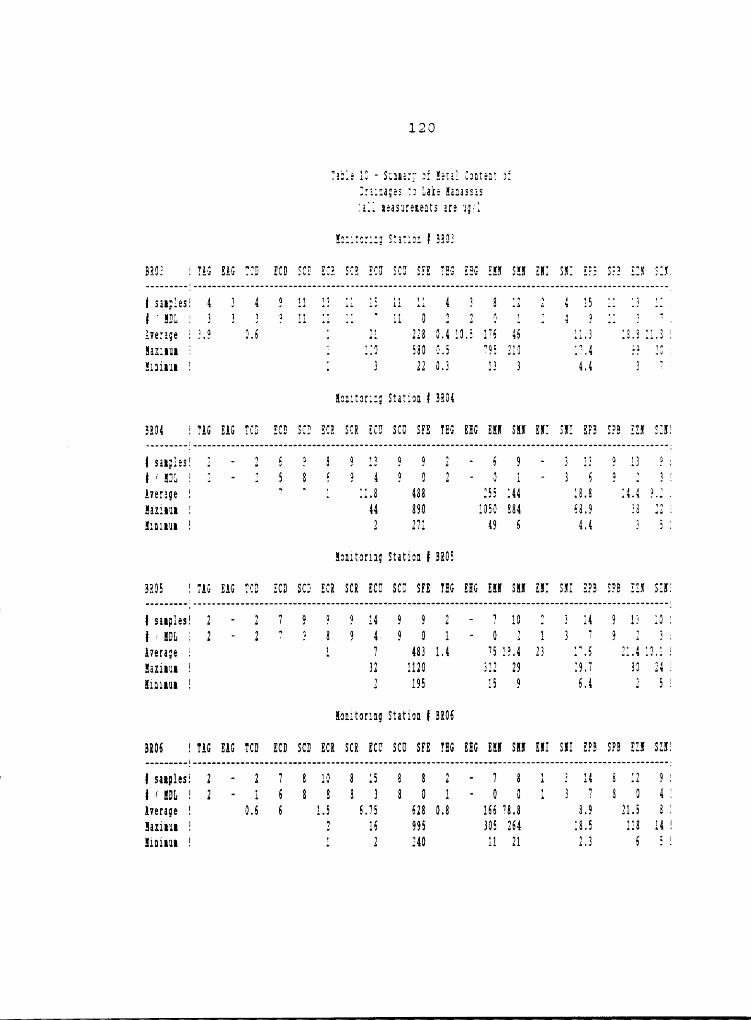
1.220

Table 13 - Sannary ai Hetal Cantent afEra;:ages to Lake Aanassasiall neasnrenents are 1g;1

!::itor;:g Stat;on 4 ER03

BR03 E EAG EAG T10 ECE ECE ECE ECE ECE SC0 SEE EEG EEG EAE SEE EE} SEC EPS SPE EZE EZE..........7 ................................................................,,.___,_,_,__________,______________

4 sanplesl 4 1 4 9 11 11 11 15 11 11 4 3 8 12 2 4 15 11 13 114 ‘ AEL 1 3 3 3 9 11 11 11 ' 11 0 2 2 0 1 Z 4 9 11 1 7Average E 3.9 0.6 1 21 228 0.4 10.5 176 46 11.3 18.8 11.8Eaxznna E 1 110 580 0.5 795 210 17.4 99 21Aaninan E 1 3 22 0.3 13 3 4.4 3 7

Aon1tor;:g Station 4 8E04

EE04 E EAG EAG ECE ECE ECE ECE SCR EC0 SC0 SEE EEG EEG EE! SEE EEI SE1 EFH SEE EZE SIE!

4 sanplesl 2 · 2 6 9 8 9 11 9 9 2 — 6 9 — 3 11 9 13 94 7 AEL E 1 - 2 5 8 6 9 4 9 0 2 - 0 1 - 3 6 9 1 3·Average 2 7 7 1 11.8 488 155 144 18.8 14.4 9.1Eaxinun E 44 890 1050 884 68.9 18 12 EEininun 1 2 271 49 6 4.4 3 5.

Eonitoring Station 4 EA05

BR05 E TAG EAG ECE EC0 SC0 ECE SCR EC0 SC0 SEE EEG EEG EHI SAE EEI SE1 EPB SEE EEE SEE!

4 sanples! 2 - 2 7 9 9 9 14 9 9 2 · 7 10 1 3 14 9 13 10 74 7 HDL E 2 — 2 7 9 8 9 4 9 0 1 - 0 2 1 3 7 9 E 1;Average E 1 7 483 1.4 75 19.4 23 17.6 11.4 10.1Eaxinun 3 32 1120 312 29 19.7 80 14~lininun 1 1 195 15 9 6.4 2 5

Eonitoring Station 4 BR06

BE06 ! TAG EAG TCD EC0 SC0 ECR SCR ECU SC0 SEE EEG EEG EAI SEE EE1 SG1 EPB SPE EZE SEE!

4 sanplesi 2 · 2 7 8 10 8 15 8 8 2 - 7 8 1 3 14 8 12 94 7 IDL ! 2 - 1 6 8 8 8 3 8 0 1 · 0 0 1 1 7 8 0 4·Average 1 0.6 6 1.5 6.75 628 0.8 166 78.8 8.9 21.5 8Eaxinun 1 2 16 995 305 264 18.5 118 14Hininun 1 1 2 240 11 21 2.1 6 5

B

1.211

Table 19 · :o:t1:ae1

!:;itcr1ng Star;on 4 9103

BR03 1 TAG EAG TCS ECS SCS ECR SCR ECS SCU SFE THG EEG EHI SAR EHI SRI AFB SPE E13 5151

4 sanplesi 4 3 4 9 11 13 11 15 11 11 4 3 8 12 2 4 15 11 13 124 1 ASL E 3 3 3 9 11 ll 11 7 11 0 2 1 0 1 2 4 9 ll 3 7Average i 3.9 0.6 1 21 Z28 1.4 10.5 176 46 11.3 15.8 11.8Ällllül 1 1 110 580 0.5 795 110 17.4 99 20Einanun E 1 3 22 0.3 13 3 4.4 3 7.

Hcnztoring Station 4 5102

5102 i TAG EAG TCD ECE SCS ECR SCR ECS SCS STE THG EEG EH! SAR SR1 SX1 ETB S25 EZ! SZR1

4 sanplesi 5 3 5 9 11 14 11 15 11 11 5 3 8 12 3 4 16 11 16 114 < HDL 1 4 3 3 9 11 14 11 6 11 0 3 2 0 2 1 4 9 11 2 7Average 1 3.6 0.3 7.7 270 1.7 1.6 246 58 27 11.5 17 32Haxrann E 0.4 13 780 2.2 1131 160 20.6 130 114Aininun E 0.2 1 35 1.2 36 22 4.4 1 5

Honitcring Station 4 5107

SR07 i TAG EAG TCS RCB SC0 ECR SCR ECU SC0 SPE THG EEG EAR SH! ER! SRI EP5 SPS EAN SZR1

4 sanp1es1 4 3 45 11 11 14 11 18 11 11 4 3 10 12 1 4 16 11 16 114 1 HDL 1 4 3 1 10 11 13 10 10 11 0 2 2 0 0 2 4 10 11 5 9Average 1 0.3 6 1 205 4 430 1.9 2.2 348 171 8 22 7.5Haxrnnn 1 0.4 8 592 975 540 18.6 106 10Hininun 1 0.1 1 50 61 32 4.4 2 5

a

122 ·

In order to further characterize the Lake Manassas

watershed, the data from station ST7O were used to develop

cumulative loading curves for various nutrients. Figures 57

through 63 are the nutrient cumulative loading curves for

the Broad Run drainage into Lake Manassas. The straight

lines represent the linear regression fits to the data

plotted. The loading data is plotted versus time in months.

The regression lines were calculated forcing them through

the origin.

123

(straight line is regression fit)18.0016.00.714.00

1s 13 12.00 1VI/\

1U vi: *0 1J :10.00 1O O¤.v» 1J1

mf 8.00 1sv1U1O 1 13 6.001

4.001112.00

'

11¤ 10.00 · J0.00 40.00 80.00 120.00Time in months

Figure 57 — ST7O loading of Orthophosphorus

124

(straight line is regression fit)

40.0066.00..1

60.00 Q°— Ivg I

° IS/$25.00Ic ‘¤

3 C I33 IC g20.00

.1:EC€15.003IlI

10.00III

5.00 I

rl0.00 '

0.00 40.00 80.00 120.00Time in months

Figure 58 — ST70 Loading of Total Soluble Phosphorus

125 .

(strcight line is regression fit)120.00 i

1IFI I100.00I

/ I“ I3 80.00 1U|,\ I

UCU

3 C I° O 0 Iag 6000EJg °1E 1E 1

3 40.00I

20.00I

Y} I0.00 ·0.00 40.00 80.00 120.00Time in months

Figure 59 - ST7O Loading of Total Phosphorus

126

60.00 (stroight line is regression fit)lII l50.00 1

Z I

in 1

° Igc40.00 1:10

Eä 1°’ ¤c 30.006 g [ IQ O9z/ p

*5 20.00 1E IE 1E I3 1‘

10.00 1I.1 I

0.00°·°° 4O-GO 80-OO 120.00Time in months

Figure 60 - ST70 Loading of Ammonia Nitrogen

II

127

(straight line is regression fit)600.00

500.00‘

Zvi l0 I

·· IU IS400,990I

°^ IviE2 I23 I·_6 3 300.00 I9 0Bf tmv ‘.2E 200.00

‘

3EEJ

U 100.00 I

0.00 Ä0.00 40.00 80.00 120.00

Time in months

Figure 61 — ST7O Loading of Oxidized Nitrogen

1I

128

(stroight Iine is regression fit)700.00 II600.00I

Z··· . I¤ 600.00IVI2 Ics0°^400.00 IC (0” E@2” :1TS ¤600.00

O .C1*;¤ I2 I0 I— 200.00 .4 I:sE IE I3 I100.00 I

0.000.00 40.00 80.00 120.00Time in months

Figure 62 · ST70 Loading of TKN

I

I

129

(straight line is regression fit)500.00Il

IZ 400.00 „ IW I° IW 1E I3 I¤^300.00 I2 3 ICDC I2 §¤ 'Q .C_C200.00 I02*2 I3 IE I8 100.00 I

III

lI0.00 I0.00 40.00 80.00 120.00

Time in months

Figure 63 — ST70 Loading of SKN

I

130

Prediction of the Eutrophic Status of Lake Manassas

As discussed in Chapter III, application of the

Vollenweider analysis for this project involved development

of a computer "spreadsheet model" of Lake Manassas.

The spreadsheet model is shown in Figure 64. The

numbers shown in Figure 64 represent the results for a given

"run" of the modeling program. The program automatically

records the results for each run for subsequent statistical

analysis.

Figures 65 and 66 represent the summary statistical

analysis for the current total phosphorus loading to the

lake using both median and average distributions. Figures

67 and 68 represent the graphical equivalents to the data

contained in Figures 65 and 66.

The output data for the total phosphorus loadings and

the z/tau hydraulic parameter for the lake are combined to

produce an "operating box" on the normal Vollenweider plot.

Figure 69 shows the "operating box" for the model output of

the currently predicted eutrophic conditions in Lake

Manassas. The box of Figure 69 represents the area of the

Vollenweider curve which, with a probability of

approximately 90%, is the current eutrophic condition of

Lake Manassas. The box is clearly well above the

"Dangerous" loading curve established by Vollenweider.

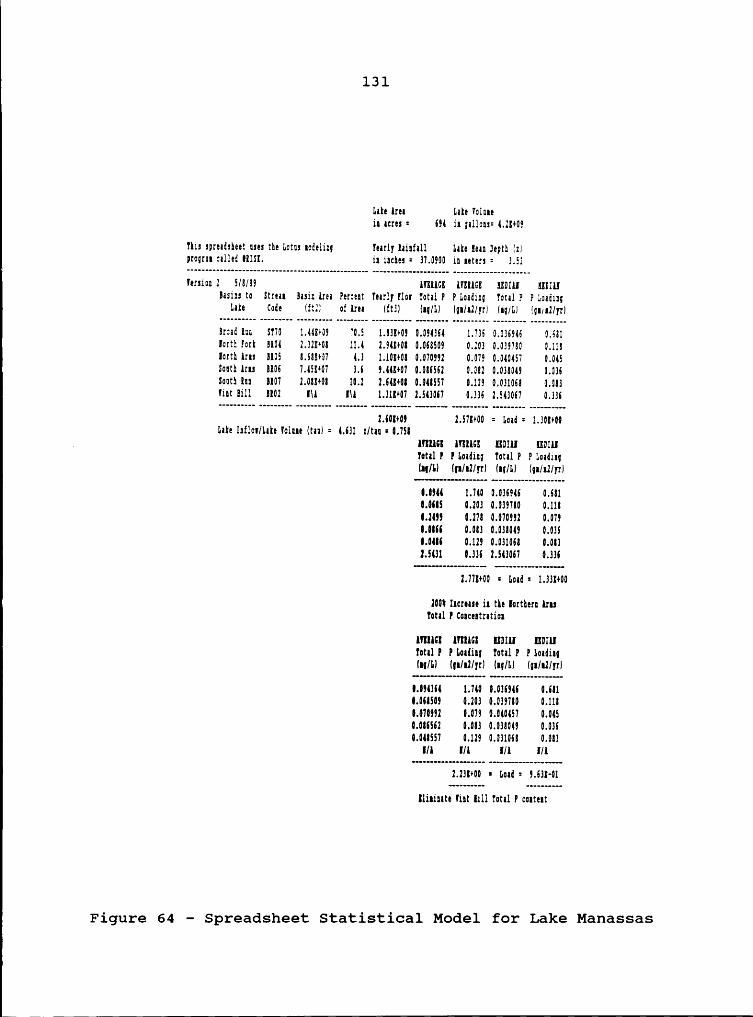
AAAAAAAA4AAA4AAAAA4AAA444AAAA4AAAA44AAAvAAY‘”_—-——————————————_—_______________________-_____----------_-—----—-

I

l 3 1

Lake Area Late 8o1unein acres = 694 in ga11ons= 4.28+09

This spreadsheet uses the Lotus nodeling Tearly Aainfall Lake 8ean 0epth IzIprograa called 08IS8. in inches = 37.0900 in neters = 3.51

Iersion 2 5/8/09 8888808 8888808 880188 880188Basins to Strean Basir Area Percent Tearly Flos Total P P Loading Total P P Loading

Lake Code Ittll ot Area Ift3I Ing/LI Iga/a2/yrI Ing/LI Ign7a2/yrIBread 8uu ST70 1.448+09 70.5 1.838+09 0.094364 1.736 0.036946 0.681Iorth Fork 8804 2.128+08 11.4 2.948+08 0.068509 0.203 0.039780 0.118Iorth Aras 8805 8.688+07 4.3 1.108+00 0.070992 0.079 0.040457 0.045South Aras 8806 7.458+07 3.6 9.448+07 0.086562 0.082 0.038049 0.036South lan 8807 2.088+08 10.2 2.648+08 0.048557 0.129 0.031068 0.0838int 8111 8802 8\8 IIA 1.318+07 2.543067 0.336 2.543067 0.336

2.608+09 2.578+00 = Load = 1.308+00Lake Infloa/Lake 8o1une ItauI = 4.631 z/tau = 0.758A 8888808 8888808 880188 880188

Total P P Loading Total P P LoadingIng/LI Iga/a2/yrI Ing/LI Iga/a2/grI0.0984 1.740 0.036986 0.6810.0605 0.203 0.039700 0.1100.2499 0.278 0.070992 0.0790.0866 0.083 0.030049 0.0360.0486 0.129 0.031068 0.0832.5438 0.336 2.543067 0.336

2.778+00 = Load = 1.338+002004 Iaorease in the Iorthern Aras

Total P Concentration

8888808 8888808 880188 I80I88Total P P Loading Total P P Loading(ag/LI (gn/a2/yrI Ina/LI Ion/a2/grI

0.094364 1.740 0.036946 0.6810.060509 0.203 0.039700 0.1180.070992 0.079 0.040457 0.0450.086562 0.003 0.038049 0.0360.048557 0.129 0.031068 0.083

8/8 8/8 8/8 8/8

2.238+00 = Load = 9.638-01

lliainate 81nt 8111 Total P content

Figure 64 - Spreadsheet Statistical Mcdel for Lake Manassas

II

132

Figure 65 - Current Average Phosphorus Loading

CURAVGLOAD QRISK Risk Analysis 08—May—1989

Expected/Mean Result = 2.625 Maximum Result = 17.05 Minimum Result = .387

Range of Possible Results = 16.666 Probability of Positive Result = 100%

Probability of Negative Result = 0% Standard Deviation = 2.149 Skeuness = 2.477 Kurtosis = 11.439

Variance = 4.620

Probability of Result > 0 = 100%> 2 = 50.7%> 4 = 16.2%> 6 = 7.6%> 8 = 2.9%> 10 = 1.8%> 12 = .8%> 14 = .3%> 16 = .2%> 18 = 0%

Probability of Result <= 0 = 0%

Percentile Probabilities: (Chance of Result < Shoun Value)< .387 = 0%< .7005 = 5%< .8637 = 10%< .9972 = 15%< 1.1463 = 20%< 1.2609 = 25%< 1.3819 = 30%< 1.5154 = 35%< 1.6509 = 40%< 1.8254 = 45%< 2.0286 = 50%< 2.196 = 55%< 2.3703 = 60%< 2.5494 = 65%< 2.7891 = 70%< 3.13 = 75%< 3.5893 = 80%< 4.2797 = 85%< 5.2896 = 90%< 6.7701 = 95%< 17.0532= 100%

1

1

Il

133

Figure 66 - Current Median Phosphorus Loading

CURMEDLOAD SRISK Risk Analysis 08-May-1989

Expected/Mean Result = 1.345 Maximum Result = 20.629 Minimum Result = .351

Range of Possible Results = 20.278 Probability of Positive Result = 100%

Probability of Negative Result = 0% Standard Deviation = 1.486 Skewness = 6.041 Kurtosis = 58.255

Variance = 2.209

Probability of Result > 0 = 100%> 2.25 = 10.3%> 4.5 = 2.9%> 6.75 = 1.5%' > 9 = .7%> 11.25 = .3%> 13.5 = .2%> 15.75 = .2%> 18 = .2%> 20.25 = .1%> 22.5 = 0%

Probability of Result <= 0 = 0%

Percentile Probabilities: < .3513 = 0%< .4652 = 5%< .5175 = 10%< .5686 = 15%< .6169 = 20%< .6648 = 25%< .7113 = 30%< .7579 = 35%< .8113 = 40%< .8665 = 45%< .935 = 50%< 1.0197 = 55%< 1.1146 = 60%< 1.204 = 65%< 1.3068 = 70%< 1.4605 = 75%< 1.644 = 80%< 1.9643 = 85%< 2.2777 = 90%< 3.3592 = 95%< 20.6293= 100%

1

134

ExpectedResult:2.625803 @RlSK Slmulotlon Som ling: Lotin H ercub

CURAVGLOAD8.0096··········

P....O

EB EA4.8%BEl E

L3.2%I

TY 1.6%01.75 3.5 5.25 7 8.75 10.5 12.25 14

Loaolng lgm P / eq. meter yrl

Figure 67 - CURAVGLOAD Output Distribution Graph

u135 l

ExpectedResult: .1.545842 @RlSK Slmulotlon Somlin: otin Hygercuéé

CURMEDLOA0 ¤Trlols:100020%P

; lR16%OE lBA

12%’’'°'°"1BEl E

' ET : _Y. ..

.,0%01.25 2.5 5.75 5 6.25 7.5 8.75 10

Loücmg (Qm P / SQ. meter vr;

Figure 68 - CURMEDLOAD Output Distribution Graph

1

136

10

EUTROP1—11C

Dangerous /

ä ä///

5 / //‘$ 1·’

- / /E // Permxsséie

E ______ __„// //E /E / /

P3 ,»·/

E Ü.lE3

OLIGOTROPHIC

0.010.1 1 10 100

Mean Dept11('Z)/Mean Residence T1I“I1€(1GLl)

Figure 69 - Vollenweider Plot of Current Conditions in Lake

Manassas

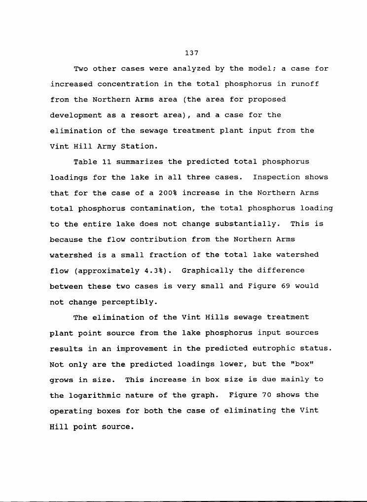
137

Two other cases were analyzed by the model; a case for

increased concentration in the total phosphorus in runoff

from the Northern Arms area (the area for proposed

development as a resort area), and a case for the

elimination of the sewage treatment plant input from the

Vint Hill Army Station.

Table 11 summarizes the predicted total phosphorus

loadings for the lake in all three cases. Inspection shows

that for the case of a 200% increase in the Northern Arms

total phosphorus contamination, the total phosphorus loading

to the entire lake does not change substantially. This is

because the flow contribution from the Northern Arms

watershed is a small fraction of the total lake watershed

flow (approximately 4.3%). Graphically the difference

between these two cases is very small and Figure 69 would

not change perceptibly.

The elimination of the Vint Hills sewage treatment

plant point source from the lake phosphorus input sources

results in an improvement in the predicted eutrophic status.

Not only are the predicted loadings lower, but the "box"

grows in size. This increase in box size is due mainly to

the logarithmic nature of the graph. Figure 70 shows the

operating boxes for both the case of eliminating the Vint

Hill point source.

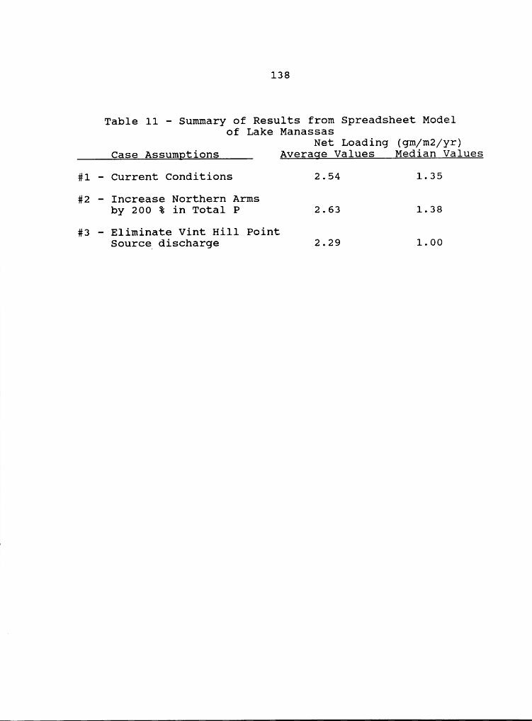
138

Table 11 - Summary of Results from Spreadsheet Modelof Lake Manassas

Net Loading (gm/m2/yr)Case Assumptions Average Values Median Values

#1 - Current Conditions 2.54 1.35

#2 - Increase Northern Armsby 200 % in Total P 2.63 1.38

#3 - Eliminate Vint Hill PointSource discharge 2.29 1.00

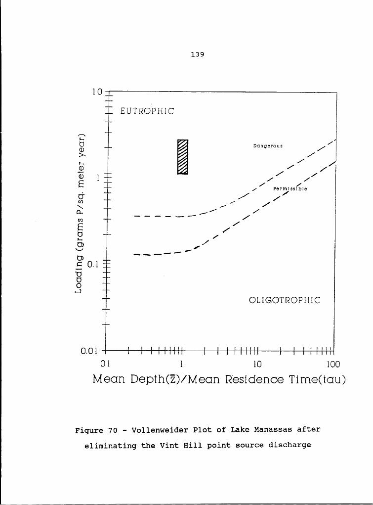
139

10

EUTROIPHIC

Donqerous //% /s.„92A / /G1 1 „’ /

E / P /_ / eryssibleS1 „/ /\/D.// /

E / /P3

//

Ö—_—.___;•¤¢

E 0.1”O .OO...1

OLIGOTROP1-IIC

0.01 ·0.1 1 10 100

Mech Depth('Z)/Mech Reskiehce "1“1me(tou)

Figure 70 - Vollenweider Plot of Lake Manassas after

eliminating the Vint Hill point source discharge

140

Table 12 represents the results of applying the other

eutrophic models discussed in Chapter III.

¤

141

Table 12 - Suumary of Other 'lrophic Models ·

Secchi Dish Surface T'P Surface Chla TSI(S) TSI (TP) TSI (Cha)

(meters) (ug/1) (ug/1)

LM01 avg 1.34 24.79 8.6 56.58 50.16 58.85

std 0.47 16.45 5.5 4.6 6.66 6.12

LM02 avg 1.31 23.13 7.6 56.7 51.9 58.85

std 0.52 17.57 5.86 4.88 5.28 5.93

H403 avg 1.22 24.17 7.33 57.81 51.55 58.84

std 0.41 17.54 4.65 4.46 6.61 4.75

LM06 avg 0.99 26.04 11.4 60.34 53.69 62.08

std 0.32 18.34 5.9 4.20 5.39 5.76

LM07 avg 0.89 32.29 9.7 62.00 53.61 60.68

std 0.24 32.16 4.6 3.58 9.84 6.07

Based on Table 4 — These data show the lake to be Eutrophic for Average Total

Phosphorus and Secchi Dish reading and Mesotrophic for Average Chlorophyll a_

Based on Table 3 — These data show the lake to be at the high end of the

mesotrophic and into the low end of the eutrophic range.

I

I

Chapter V

DISCUSSION

Discussion of Monitoring Program Results for Lake Manassas

Table 7 lists the morphological characteristics of Lake

Manassas as measured for this thesis. The volume of 4.2

billion gallons agrees well with some previous studies (1).

The lake was originally designed for a volume of

approximately 5.8 billion gallons. However, the original

engineering company which designed the lake has recently

performed another study to measure the lake's volume.

Although the results of that study were not available at the

time this thesis was written, unofficial results confirm

that the lake's volume is closer to a figure of 4.2 billion

gallons (2).

The temperature profile data, Figures 7 through 14,

show that Lake Manassas is a monomictic lake, with typical

fall turnovers. The summer stratification is very evident,

especially in the deeper portions of the lake. There is no

quantifiable winter stratification, however when ice is

present, sampling is not performed. This unavailable data

makes it difficult to make conclusive statements regarding

winter stratification.

142

1I

143'

Figures 8, 9, 11, and 12 show that at depths of over 30

feet (the hypolimnion) the temperature rarely, if ever,

rises above 10b. These figures also show that during

periods of turnover, the entire water column reaches a

temperature of 10%L

Figures 9, 12, 13, and 14 are useful for characterizing

the epilimnion of Lake Manassas. These figures show that

the epilimnion extends to a depth of 12 to 15 feet during

the summer months. Figure 12 shows that at Station LMO6,

there is almost no stratification to a depth of 15 feet in

the summer months. Figure 9 shows that at Station LMO3

there is an approximately TC layer at 15 feet. This

difference may be due to the location of the two stations.

Station LMO3 is at the end of a narrow arm of the lake,

whereas Station LM06 is in the center of a relatively broad

section of the lake and is significantly further from land.

Therefore, wind forces on the lake at LM06 may induce better

mixing conditions than at LMO3. Given the small thermal

gradient present between the surface and 15 feet, this small

difference in wind mixing force would probably be enough to

account for the difference between LM06 and LMO3.

The DO contour figures further confirm these

conclusions, and provide further insight into Lake Manassas

dynamics. Figures 15 through 22 provide the DO contours,

1144

and Figures 23 through 30 the percent of DO saturation

contours. Figures 15, 16, and 18 clearly show the

stratification of DO in the water column of the lake. DO

levels in the epilimnion during summer months typically

exceed 10 mg/L. Figures 23, 24, and 26 confirm that these

DO levels are at or above the saturation level of DO,

corrected for actual temperature at that location. This

pattern of DO content indicates that oxygen producing,

photosynthetic organisms are prolific during the summer

months. Therefore, the addition of copper sulfate to the

lake during the spring and fall may help reduce the

magnitude of the spring and fall algal blooms, it does not

strongly affect the warm season algal crop.

The transition from epilimnion to hypolimnion is more

dramatic on the %DO saturation contour figures. Figures 23,

24, and 26 show that at a depth of 11 to 12 feet, the % DO

saturation begins to change rapidly with depth.

Referring to Figure 6, a depth of 12 feet corresponds

to an elevation of 273 feet above mean sea level, or a lake

volume of 2.0 billion gallons. Therefore, the epilimnion

volume is estimated at (4.2 — 2.0) or 2.2 billion gallons,

and comprises approximately 52% of the lake volume.

Figures 31 through 34 also clearly depict the

hypolimnion DO conditions. Figure 31 clearly shows that DO

145

at the lake bottom of station LMO1 essentially goes to zero.

This means that anaerobic conditions are quite prevalent for

the 4 to 5 month summer period. Figures 31 through 34 also

clearly show the mixing periods of lake turnover.

Figures 33 and 34 are the top and bottom DO curves for

station LMO8. For the two year monitoring period contained

in the database, the top and bottom DO concentrations at

LMO8 showed little difference except for a 6 month period in

the summer of 1986, when some stratification did occur.

However, the conditions were not as severe as in deeper' portions of the lake. The lowest DO concentration reached

was 3.3 mg/L which corresponded to a 40% DO saturation

level.

Figures 35 through 42 present the data for

chlorophyll g in the surface waters at the sampling points.

The data clearly show the presence of chlorophyll g at all

locations in the lake. The peaks do not always concur at

the same time of year or at the same date from location to

location. This time disparity may be due to the addition of

copper sulfate to the lake, the difference in time between

sampling and the copper sulfate addition, and the

nonuniformity of the copper sulfate addition.

Figures 43 through 45 are a different presentation

technique for the chlorophyll a data. Figure 43 shows that

146

the chlorophyll Q concentration at stations LMO1 and LMO3

behave very similarly. The maximum peaks are very similar

in magnitude. The time at which the maximum occurs is,

however, different. Figure 44 is a comparison of the

chlorophyll Q at stations LMO1 and LMO6. The chlorophyll Q

at LMO6 has slightly higher peaks, but, more predominantly,

a higher average concentration. This is most likely due to

the better availability of nutrients in the area around LMO6

from South Run. Figure 45 is a comparison of chlorophyll Q

at LMO6 and LMO7. This figure shows that LMO6 is a more

productive region for chlorophyll Q than is LMO7. This may

not be expected because LMO7 is a shallow area, and the

better light penetration should help produce more littoral

communities at LMO7. However, the better availability of

nutrients at LMO6 has a stronger affect on the net

productivity.

Figures 46, 47, and 48 are plots of the ammonia and

oxidized nitrogen in the bottom waters of LMO1, LMO6 and

LMO7. The pattern of the data is quite evident. The

oxidized nitrogen follows a cyclical pattern, with the

ammonia nitrogen cycle being in an exactly opposite phase

pattern. However, there is a distinct difference between

the data from LMO1, and that from LMO6 and LMO7. At LMO6

and LMO7, the oxidized nitrogen peaks are substantially

147

higher than expected for the amount of ammonia present. At

LM01, the ammonia peaks correspond with fall turnover, and

the oxidized nitrogen level which follows does not

correspond to the peak value expected. The major difference

between LMO1 and the other stations is depth. Note that

when corrected for scale differences, the peak values of

oxidized nitrogen at all three stations is very similar.

Therefore, it appears that either the sediment releases

oxidized nitrogen at LMO1, or, at the shallow depths of LMO6

and LMO7, the ammonia adsorption to sediment and the

nitrification reaction may be great enough to keep the

ammonia concentration very low.

Figure 49 is a top and bottom plot of oxidized nitrogen

at station LMO1. The plot shows a clear agreement between

oxidized nitrogen in the top and bottom waters of LMO1.

There is a cyclical pattern, with peaks in the spring and

early summer, and lows in late summer and fall. There is no

apparent difference in magnitude or periodicity between the

top and bottom waters.

Figures 50 and 51 are plots of the bottom

concentrations of total nitrogen and total phosphorus at

stations LM01 and LMO6. The plots show periodicity

agreement between the nitrogen and phosphorus in the bottom

waters at these locations. The relative magnitudes are

148 Fdifferent, which is as expected because the two parameters

are not related.

Figures 52 and 53 are plots of the various phosphorus

parameters in the bottom waters of LMO1 and LMO6. The plots

show that the total phosphorus is about twice the value of

the total soluble phosphorus.

Figure 54 is a plot of the total phosphorus in the

surface waters of LMO1, LMO3, and LMO6. This graph shows no

apparent difference between the peak concentrations at LMO1,

LMO3, and LMO6. However, the average concentration at LMO6

does appear to be higher than the other two locations. This

corresponds with the chlorophyll Q data of Figures 43 and

44. Also, there appears to be a trend in the data towards a

lower average phosphorus concentration at all the sample

locations over the monitoring period analyzed. This trend

follows Figure 55 which shows a decreasing rainfall rate

over the same monitoring period analyzed.

Inspection of Figure 55 clearly shows that as yearly

rainfall increases, the amount of runoff increases. This

observation makes sense because consistently wet conditions

indicate the soil will be saturated more often, encouraging

runoff. Figures 54, 55 and 56 indicate a strong connection

between the rainfall rate and the amount of phosphorus

present in the lake. This confirms the connection between

11

149

the lake and its watershed: it is unlikely that there are

other substantial sources of nutrients into the lake.

Figure 56 shows that as rainfall rate increases, so

does the amount of runoff. As stated previously, this

observation is also fundamental. The predicted values for

percent runoff agree well with the long term runoff rate of

35%, measured by the U.S. Geological Survey in the

region.(30)

Discussion of Monitoring Program Results for the Lake

Manassas Watershed

Table 9 summarizes the conventional and nutrient

monitoring data for the various surface water drainages into

Lake Manassas. The first observation is the adverse impact

of the Vint Hill treatment plant discharge on the quality of

the water in South Run. South Run at station BRO2 contains

significant quantities of both phosphorus and oxidized

nitrogen. There is not a substantial increase in ammonia

nitrogen. Therefore, the Vint Hill treatment plant does

appear to have an efficient nitrification system.

Some general conclusions for the lake's drainages can

be made:

150

1. The pH values of the drainages are at or

slightly below neutrality. None of the drainages

differ significantly in the parameter.

2. The average and median total suspended solids

concentration values appear to be low; some high values

do appear, but are generally associated with storm

events. Typical average values between 8 and 20 mg/L

and typical median values of 7 mg/L. Maximum values

ranged from 80 mg/L to 383 mg/L.

3. The dissolved oxygen content of all thei

streams is near saturation, with typical median and

average values above 87% saturation. Station BR03 had

the highest maximum at 177% saturation. This data

indicates that (a) the biological oxygen demand in the

streams is not large enough to produce an oxygen

deficit, and (b) photosynthesis is occurring in the

streams.

4. The conventional nutrient concentrations in

all the streams are similar, except in South Run.

Average and median total phosphorus concentrations

correspond closely between the streams with values from

0.05 to .10 mg/L. In contrast BR02, the Vint Hill

discharge, has an average and median value between 0.10

and 0.20 mg/L. The maximum observed total phosphorus

151

at BRO2 was 0.82 mg/L, over twice the maximum observed

in any other stream. However, oxidized nitrogen at the

BRO2 station is the most significant nutrient.

Oxidized nitrogen at BRO2 has an average of 1.93 mg/L

and median value of 0.58 mg/L. These values are

between a factor of 5 and 10 times higher than the

other stations. Ammonia nitrogen is not significantly

higher in BRO2 than other stations with an average and

median value of 0.17 and 0.02 mg/L respectfully.

Table 10 summarizes the metal pollutant monitoring

data for the various surface water drainages into Lake

Manassas. In general, inspection of the data shows no

significant metal pollution in any of the drainages into

Lake Manassas. Only iron, copper, manganese, and zinc

appear consistently at concentrations well above detection

limits, however, these metals are found commonly in soil

(15). The high levels of these metals correspond with

periods of high total suspended solids, indicating the

connection between the metal content and the sediment

entrained in the stream flow. Most of the other metals were

not detected above their respective detectable limits. One

exception is lead, which was detected in about half of the

samples for which it was analyzed, with an average value of

11

152

20 ug/L. Most of the detectable lead concentations occurred

in the early dates of the sample period. The lack of lead

being detectable in the later samples may be an indication

of the effectiveness of unleaded gasolines. .

Figures 57 through 63 represent the cumulative loadings

curves for the conventional nutrients from Broad Run (ST70).

The curves show some cyclic behavior, related to the

rainfall patterns. However, in general the plots show that

the loading curves follow a straight line quite closely.

This indicates that the magnitude of the nutrient input from

the Broad Run watershed did not change over the monitoring

period.

Discussion of the Modeling Results Predicting the Eutrophic

Status of Lake Manassas

Application of the Vollenweider model to Lake Manassas

shows that the lake is eutrophic, with the yearly phosphorus

loading rate well above the "dangerous" curve as defined by

Vollenweider. The computer model developed for Lake

Manassas predicts a small effect on the overall quality of

the water in the lake if the runoff from the Northern Arms

area of the lake changes substantially. The predicted

changes in the lake's eutrophic status would probably not be

detectable in the lake, but monitoring the runoff into the

1

153

lake should detect any adverse effects. There could be a

localized increase in the algae growth of the Northern Arm,

similar to the behavior of LM06 versus the rest of the lake.

Elimination of the major point source to the lake, the Vint

Hill sewage treatment plant, would have a more pronounced

effect, but it would not lower the predicted phosphorus

loading rate below the "dangerous" curve.

Application of the other eutrophic index models shows

the lake to be either very high in the mesotrophic range or

well into the eutrophic range, depending on which parameter

is used for indexing. Most of the parameters indicate that

the lake is eutrophic. In particular, the Carlson TSI

method shows the lake does tend toward the eutrophic region,

based on the historical data.

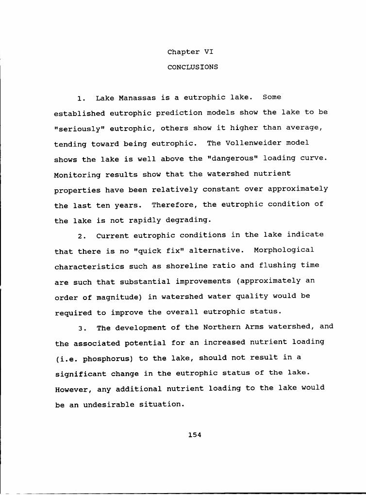
1I

Chapter VI

CONCLUSIONS

1. Lake Manassas is a eutrophic lake. Some

established eutrophic prediction models show the lake to be

"seriously" eutrophic, others show it higher than average,

tending toward being eutrophic. The Vollenweider model

shows the lake is well above the "dangerous" loading curve.

Monitoring results show that the watershed nutrient

properties have been relatively constant over approximately

the last ten years. Therefore, the eutrophic condition of

the lake is not rapidly degrading.

2. Current eutrophic conditions in the lake indicate

that there is no "quick fix" alternative. Morphological

characteristics such as shoreline ratio and flushing time

are such that substantial improvements (approximately an

order of magnitude) in watershed water quality would be

required to improve the overall eutrophic status.

3. The development of the Northern Arms watershed, and

the associated potential for an increased nutrient loading

(i.e. phosphorus) to the lake, should not result in a

significant change in the eutrophic status of the lake.

However, any additional nutrient loading to the lake would

be an undesirable situation.

154

fl

i

155

4. The addition of copper sulfate to the lake may help

minimize the peak values of spring and fall algae blooms.

However, this chemical addition does not have a substantial

affect on the overall net biomass production.

5. The current monitoring program established for Lake

Manassas and its watershed is sufficient for tracking the

lake's status. The monitoring program adequately monitors

both the significant point and non-point sources to the

lake.

Chapter VII

RECOMMENDATIONS

1. The computer model developed for predicting the

eutrophic status of Lake Manassas could be improved by

incorporating the effects of the withdrawal-refill cycle

normally associated with reservoirs. The existing

environmental monitoring database contains a field for pool

elevation in the lake. Recording the value of this

parameter during environmental sampling would enable this

improvement to the computer model to be made.

2. In order to better understand the absolute affects

of the copper sulfate addition, it may be desirable to

devise an experiment where one of the smaller arms of the

lake actually not be treated with the other arms of the

lake. The chlorophyll Q concentration in the untreated arm

could then be compared to the treated arms. If this type of

experiment is considered to be too risky, perhaps a sliding

scale of copper sulfate dose could be developed with

commensurate chlorophyll Q monitoring. This type of

experiment could help to better quantify the benefits of

copper sulfate addition.

3. The policies of nutrient control within the Lake

Manassas watershed (as part of the greater Occoquan

156

uuu

157

Watershed) should continue to be observed and enforced.

Further degradation of the watershed water quality will only

magnify an existing unsatisfactory situation.

4. Further research into sediment—water interactions

may help develop a methodology to minimize nutrient release

from the sediments in the lake.

Chapter VIII

REFERENCES CITED

1. Laufer, Susan M., "Nutrient Dynamics in the Lake Manassas(Virginia) Watershed." M.S. Thesis, Virginia PolytechnicInstitute and State University, Blacksburg, VA (1986).

2. Whetzel, Wade, Chief Operator, City of Manassas WaterTreatment Plant, Greenwich, Virginia, personal interview.

3. Commonwealth of Virginia State Water Control Board, Policyfor· Waste‘ Treatment and ‘Water* Quality Management in. theOccoguan Watershed, State of Virginia, Document Number RC-4-1, revised December 12, 1980.

4. Jones-Saunders Associates, "Residential Planned CommunityZoning Report, Robert Trent Jones International, PrinceWilliam County, Virginia, Chatham, New Jersey (1986)."

5. Northern Virginia Planning District Commission, "NonpointPollution Analysis of the Robert Trent Jones InternationalRezoning Proposal." Final Report..Annandale, Virginia (1986).

6. Whetzel, Robert G., Limnology, Second Edition, SaundersCollege Publishing, New York, NY, 767 pp. (1983).

7. Welch, Paul S., Limnological Methods, McGraw—Hill BookCompany, Inc., New York, NY, 370 pp. (1948).

8. Boyd, Claude E., Water Quality in Warmwater Fish Ponds,Craftmaster Printers Inc., Opelika, AL, 359 pp. (1979).

9. Odum, Eugene P., Fundamentals of Ecology, Second Edition,W.B. Saunders Company, Philadelphia, PA, 574 pp. (1971).

10. Falkenborg, Donna H., Maloney, Thomas E., Middlebrooks,E. Joe, Modeling the Eutrophication Process, Ann Arbor SciencePublishers Inc., Ann Arbor, MI, 213 pp. (1974).

11. Marvan, P., Pribil, S., Lhotsky, O., Algal Assays andMonitoring Eutrophication, E. Schweizerbart'scheVerlagsbuchhandlung (Nagele 11. Obermiller), Stuttgart, W.Germany, 253 pp. (1979).

158

159

12. Averett, Robert C., McKnight, Diane M., Chemical QualityWater and the Hydrologic Cycle, Lewis Publishers, Inc.,Chelsea, MI, 382 pp. (1987).

13. dewit, C.T., Goudriaan, J., Simulation of EcologicalProcesses, John Wiley & Sons, New York, NY, 174 pp. (1978).

14. Rohlich, Gerald A., Eutrophication: Causes, Conseguences,Correctives, Proceedings of a Symposium, National Academy ofSciences, Washington, DC, 661 pp. (1969).

15. Connell, D.W., Miller G.J., Chemistry and Ecotoxicologyof Pollution, John.‘Wiley' & Sons, New' York, NY, 444 pp.(1984).

16. Benefield, L.D., Randall C.W., Biological Process Designfor Wastewater Treatment, Teleprint Publishing Inc.,Charlottesville, VA, 526 pp. (1985).

17. Chan. E.C.S., Pelczar, Michael J. Jr., Krieg, Noel R.,Microbiology, McGraw-Hill Book Company, New York, NY, 918 pp.(1986).

18. Eckenfelder, W. Wesley Jr., Principles of Water QualityManagement, CBI Publishing Company Inc., Boston, MS, 717 pp.(1980).

19. Orten, James M., Neuhaus, Otto W., Biochemistry, TheC.V. Mosby Company, Saint Louis, MS, 925 pp. (1970).

20. Dillon, P.J., "The Application of the Phosphorus LoadingConcept to Eutrophication Research." Canada Centre for InlandWaters, Burlington, Ontario, 28 pp. (1976).

21. Grizzard, T.J., Randall, C.W., Sherman, T.E., Weand,B.W., and Hoehn, R.C., "Management of Sediment PhosphorusCycling by Nitrate Addition." Paper presented at Congres dansles Eaux, Paris, France, October 22-24, 1985.

22. Carlson, IL ‘E., "A Trophic State Index for Iakes."Limnology and Oceanography, gg, 361-369 (1977).

23. Reckhow, K.H., "Quantitative Techniques for theAssessment of Lake Quality." Office of water Planning andStandards, EPA-440/5-79-015, USEPA, Washington, DC (1979).

24. Grizzard, Thomas J., Director, Occoquan WatershedMonitoring Laboratory, Manassas, VA, personal communication.

l6O ~

n

25. Tasker, G.D., Driver, N.E., "Nationwide Regression Modelsfor Predicting Urban Runoff Water Quality at UnmonitoredSites," Water Resources Bulletin, American Water ResourcesAssociation, Vol. 24, No.5, October 1988, p. 1091.

26. Northern Virginia Planning District Commission,"Washington Metropolitan Area Urban Runoff DemonstrationProject," Final Report, April, 1983.

27. Breed, Charles B., Hosmer, George L., ElementarySurveying, John Wiley & Sons Inc., New York, NY, 717 p.(1958).

28. U.S. Geological Survey, U.S. Department of Interior, andthe Commonwealth of Virginia Division of Mineral Resources,7.5 Minute Series Topographic Maps for the following Virginiaquadrangles; Throughfare Gap (1983), Gainesville (1983),Middleburg (1978), Rectortown (1981), Marshall (1983), Catlett(1978), and Warrenton (1978).

29. Dymond R.L., McDonnell, A.J., "Determination of Ungaged_ Tributary Flows and Intersegmental Reservoir Flows using

Spreadsheet Software", Water' Resources Bulletin, AmericanWater Resources Association, Vol. 24, No. 5, October 1988, p.1065.

30. Water Resources Data — Virginia, Water Year 1985, U.S.Geological Survey Water Data Report VA-85-1.