Embed Size (px)
Citation preview

Probability Distributions
Brenda Meery, (BrendaM)CK12 Editor
Say Thanks to the AuthorsClick http://www.ck12.org/saythanks
(No sign in required)

To access a customizable version of this book, as well as otherinteractive content, visit www.ck12.org
CK-12 Foundation is a non-profit organization with a mission toreduce the cost of textbook materials for the K-12 market bothin the U.S. and worldwide. Using an open-content, web-basedcollaborative model termed the FlexBook®, CK-12 intends topioneer the generation and distribution of high-quality educationalcontent that will serve both as core text as well as provide anadaptive environment for learning, powered through the FlexBookPlatform®.
Copyright © 2012 CK-12 Foundation, www.ck12.org
The names “CK-12” and “CK12” and associated logos and theterms “FlexBook®” and “FlexBook Platform®” (collectively“CK-12 Marks”) are trademarks and service marks of CK-12Foundation and are protected by federal, state, and internationallaws.
Any form of reproduction of this book in any format or medium,in whole or in sections must include the referral attribution linkhttp://www.ck12.org/saythanks (placed in a visible location) inaddition to the following terms.
Except as otherwise noted, all CK-12 Content (includingCK-12 Curriculum Material) is made available to Usersin accordance with the Creative Commons Attribution/Non-Commercial/Share Alike 3.0 Unported (CC BY-NC-SA) License(http://creativecommons.org/licenses/by-nc-sa/3.0/), as amendedand updated by Creative Commons from time to time (the “CCLicense”), which is incorporated herein by this reference.
Complete terms can be found at http://www.ck12.org/terms.
Printed: September 19, 2012
AUTHORSBrenda Meery, (BrendaM)CK12 Editor
www.ck12.org Chapter 1. Probability Distributions
CHAPTER 1 Probability DistributionsCHAPTER OUTLINE
1.1 Normal Distributions
1.2 Binomial Distributions
1.3 Exponential Distributions
1.4 Review Questions
Introduction
For a standard normal distribution, the data presented is continuous. In addition, the data is centered at the mean andis symmetrically distributed on either side of that mean. This means that the resulting data forms a shape similar toa bell and is, therefore, called a bell curve. Binomial experiments are discrete probability experiments that involvea fixed number of independent trials, where there are only 2 outcomes. As a rule of thumb, these trials result insuccesses and failures, and the probability of success for one trial is the same as for the next trial (i.e., independentevents). As the sample size increases for a binomial distribution, the resulting histogram approaches the appearanceof a normal distribution curve. With this increase in sample size, the accuracy of the distribution also increases. Anexponential distribution is a distribution of continuous data, and the general equation is in the form y = abx. Thecloser the correlation coefficient is to 1, the more likely the equation for the exponential distribution is accurate.
1
1.1. Normal Distributions www.ck12.org
1.1 Normal Distributions
Learning Objectives
• Be familiar with the standard distributions (normal, binomial, and exponential).• Use standard distributions to solve for events in problems in which the distribution belongs to one of these
families.
In Chapter 3, you spent some time learning about probability distributions. A distribution, itself, is simply adescription of the possible values of a random variable and the possible occurrences of these values. Remember thatprobability distributions show you all the possible values of your variable (X), and the probability associated witheach of these values (P(X)). You were also introduced to the concept of binomial distributions, or distributions ofexperiments where there are a fixed number of successes in X (random variable) trials, and each trial is independentof the other. In addition, you were introduced to binomial distributions in order to compare them with multinomialdistributions. Remember that multinomial distributions involve experiments where the number of possible outcomesis greater than 2, and the probability is calculated for each outcome for each trial.
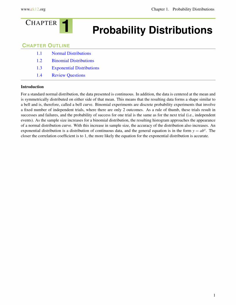
In this first lesson on probability distributions, you are going to begin by learning about normal distributions. Anormal distribution curve can be easily recognized by its shape. The first 2 diagrams above show examples ofnormal distributions. What shape do they look like? Do they look like a bell to you? Compare the first 2 diagramsabove to the third diagram. A normal distribution is called a bell curve because its shape is comparable to a bell. It
2

www.ck12.org Chapter 1. Probability Distributions
has this shape because the majority of the data is concentrated at the middle and slowly decreases symmetrically oneither side. This gives it a shape similar to a bell.
Actually, the normal distribution curve was first called a Gaussian curve after a very famous mathematician, CarlFriedrich Gauss. He lived between 1777 and 1855 in Germany. Gauss studied many aspects of mathematics. Oneof these was probability distributions, and in particular, the bell curve. It is interesting to note that Gauss also spokeabout global warming and postulated the eventual finding of Ceres, the planet residing between Mars and Jupiter. Aneat fact about Gauss is that he was also known to have beautiful handwriting. If you want to read more about CarlFriedrich Gauss, look at http://en.wikipedia.org/wiki/Carl_Friedrich_Gauss.
In Chapter 3, you also learned about discrete random variables. Remember that discrete random variables are onesthat have a finite number of values within a certain range. In other words, a discrete random variable cannot take onall values within an interval. For example, say you were counting from 1 to 10. You would count 1, 2, 3, 4, 5, 6,7, 8, 9, and 10. These are discrete values. 3.5 would not count as a discrete value within the limits of 1 to 10. Fora normal distribution, however, you are working with continuous variables. Continuous variables, unlike discretevariables, can take on any value within the limits of the variable. So, for example, if you were counting from 1 to 10,3.5 would count as a value for the continuous variable. Lengths, temperatures, ages, and heights are all examplesof continuous variables. Compare these to discrete variables, such as the number of people attending your class, thenumber of correct answers on a test, or the number of tails on a coin flip. You can see how a continuous variablewould take on an infinite number of values, whereas a discrete variable would take on a finite number of values. Asyou may know, you can actually see this when you graph discrete and continuous data. Look at the 2 graphs below.The first graph is a graph of the height of a child as he or she ages. The second graph is the cost of a gallon ofgasoline as the years progress.
3

1.1. Normal Distributions www.ck12.org
If you look at the first graph, the data points are joined, because as the child ages from birth to age 1, for example, hisheight also increases. As he continues to age, he continues to grow. The data is said to be continuous and, therefore,you can connect the points on the graph. For the second graph, the price of a gallon of gas at the end of each yearis recorded. In 1930, a gallon of gas cost 10�c. You would not have gone in and paid 10.2�c or 9.75�c. The data is,therefore, discrete, and the data points cannot be connected.
Let’s look at a few problems to show how histograms approximate normal distribution curves.
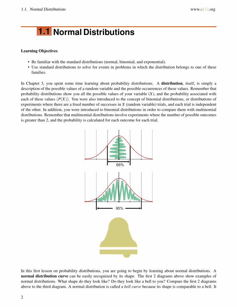
Example 1
Jillian takes a survey of the heights of all of the students in her high school. There are 50 students in her school. Sheprepares a histogram of her results. Is the data normally distributed?
Solution:
If you take a normal distribution curve and place it over Jillian’s histogram, you can see that her data does notrepresent a normal distribution.
If the histogram were actually shaped like a normal distribution, it would have a shape like the curve below:
4
www.ck12.org Chapter 1. Probability Distributions
Example 2
Thomas did a survey similar to Jillian’s in his school. His high school had 100 students. Is his data normallydistributed?
Solution:
If you take a normal distribution curve and place it over Thomas’s histogram, you can see that his data also does notrepresent a normal distribution.
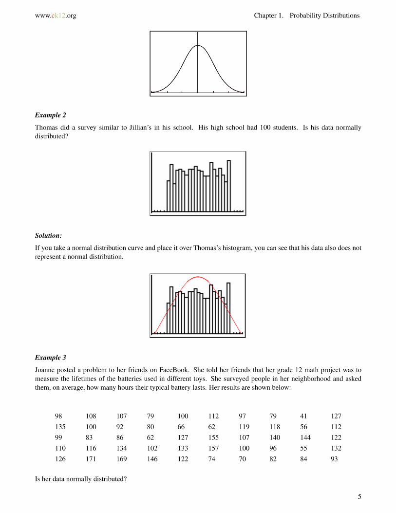
Example 3
Joanne posted a problem to her friends on FaceBook. She told her friends that her grade 12 math project was tomeasure the lifetimes of the batteries used in different toys. She surveyed people in her neighborhood and askedthem, on average, how many hours their typical battery lasts. Her results are shown below:
98 108 107 79 100 112 97 79 41 127
135 100 92 80 66 62 119 118 56 112
99 83 86 62 127 155 107 140 144 122
110 116 134 102 133 157 100 96 55 132
126 171 169 146 122 74 70 82 84 93
Is her data normally distributed?
5

1.1. Normal Distributions www.ck12.org
Solution:
If you take a normal distribution curve and place it over Joanne’s histogram, you can see that her data appears tocome from a normal distribution.
This means that the data fits a normal distribution with a mean around 105. Using the TI-84 calculator, you canactually find the mean of this data to be 105.7.
What Joanne’s data does tell us is that the mean score (105.7) is at the center of the distribution, and the data fromall of the other scores (times) are spread from that mean. You will be learning much more about standard normaldistributions in a later chapter. But for now, remember the 2 key points about a standard normal distribution. Thefirst key point is that the data represented is continuous. The second key point is that the data is centered at the meanand is symmetrically distributed on either side of that mean.
Standard normal distributions are special kinds of distributions and differ from the binomial distributions you learnedabout in the last chapter. Let’s now take a more detailed look at binomial distributions and see how they differdramatically from the standard normal distribution.
6

www.ck12.org Chapter 1. Probability Distributions
1.2 Binomial Distributions
In the last chapter, you found that binomial experiments are ones that involve only 2 choices. Each observationfrom the experiment, therefore, falls into the category of a success or a failure. For example, if you tossed a cointo see if a 6 appears, it would be a binomial experiment. A successful event is the 6 appearing. Every other roll (1,2, 3, 4, or 5) would be a failure. Asking your classmates if they watched American Idol last evening is an exampleof a binomial experiment. There are only 2 choices (yes and no), and you can deem a yes answer to be a successand a no answer to be a failure. Coin tossing is another example of a binomial experiment, as you saw in Chapter3. There are only 2 possible outcomes (heads and tails), and you can say that heads are successes if you are lookingto count how many heads can be obtained. Tails would then be failures. You should also note that the observationsare independent of each other. In other words, whether or not Alisha watched American Idol does not affect whetheror not Jack watched the show. In fact, knowing that Alisha watched American Idol does not tell you anything aboutany of your other classmates. Notice, then, that the probability for success for each trial is the same.
The distribution of the observations in a binomial experiment is known as a binomial distribution. For binomialexperiments, there is also a fixed number of trials. As the number of trials increases, the binomial distributionbecomes closer to a normal distribution. You should also remember that for normal distributions, the random variableis continuous, and for binomial distributions, the random variable is discrete. This is because binomial experimentshave 2 outcomes (successes and failures), and the counts of both are discrete.
Of course, as the sample size increases, the accuracy of a binomial distribution also increases. Let’s look at anexample.
Example 4
Keith took a poll of the students in his school to see if they agreed with the new “no cell phones” policy. He foundthe following results.
TABLE 1.1:
Age Number Responding No14 5615 6516 9017 9518 60
Solution:
Keith plotted the data and found that it was distributed as follows:
Clearly, Keith’s data is not normally distributed.
7

1.2. Binomial Distributions www.ck12.org
Example 5
Jake sent out the same survey as Keith, except he sent it to every junior high school and high school in the district.These schools had students from grade 6 (age 12) to grade 12 (up to age 20). He found the following data:
TABLE 1.2:
Age Number Responding No12 27413 26114 25915 28916 23317 22518 25319 24520 216
Solution:
Jake plotted his data and found that the data was distributed as follows:
Because Jake expanded the survey to include more people (and a wider age range), his data turned out to fit moreclosely to a normal distribution.
Notice that in Jake’s sample, the number of people responding no on the survey was 2,225. This number has a hugeadvantage over the number of students who responded no on Keith’s survey, which was 366. You can make muchmore accurate conclusions with Jake’s data. For example, Jake could say that the biggest opposition to the new “nocell phones” policy came from the middle or junior high schools, where students were 12–15 years old. This is notthe same conclusion Keith would have made based on his small sample.
In Chapter 3, you did a little work with the formula used to calculate probability for binomial experiments. Here isthe general formula for finding the probability of a binomial experiment from Chapter 3.
The probability of getting X successes in n trials is given by:
P(X = a) = nCa × pa ×q(n−a)
where:
a is the number of successes from the trials.
p is the probability of success.
q is the probability of failure.
Let’s look at a simple example of a binomial probability distribution just to recap what you learned in Chapter 3.
8
www.ck12.org Chapter 1. Probability Distributions
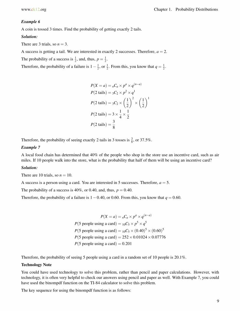
Example 6
A coin is tossed 3 times. Find the probability of getting exactly 2 tails.
Solution:
There are 3 trials, so n = 3.
A success is getting a tail. We are interested in exactly 2 successes. Therefore, a = 2.
The probability of a success is 12 , and, thus, p = 1
2 .
Therefore, the probability of a failure is 1− 12 , or 1
2 . From this, you know that q = 12 .
P(X = a) = nCa × pa ×q(n−a)
P(2 tails) = 3C2 × p2 ×q1
P(2 tails) = 3C2 ×(
12
)2
×(
12
)1
P(2 tails) = 3× 14× 1
2
P(2 tails) =38
Therefore, the probability of seeing exactly 2 tails in 3 tosses is 38 , or 37.5%.
Example 7
A local food chain has determined that 40% of the people who shop in the store use an incentive card, such as airmiles. If 10 people walk into the store, what is the probability that half of them will be using an incentive card?
Solution:
There are 10 trials, so n = 10.
A success is a person using a card. You are interested in 5 successes. Therefore, a = 5.
The probability of a success is 40%, or 0.40, and, thus, p = 0.40.
Therefore, the probability of a failure is 1−0.40, or 0.60. From this, you know that q = 0.60.
P(X = a) = nCa × pa ×q(n−a)
P(5 people using a card) = 10C5 × p5 ×q5
P(5 people using a card) = 10C5 × (0.40)5 × (0.60)5
P(5 people using a card) = 252×0.01024×0.07776
P(5 people using a card) = 0.201
Therefore, the probability of seeing 5 people using a card in a random set of 10 people is 20.1%.
Technology Note
You could have used technology to solve this problem, rather than pencil and paper calculations. However, withtechnology, it is often very helpful to check our answers using pencil and paper as well. With Example 7, you couldhave used the binompdf function on the TI-84 calculator to solve this problem.
The key sequence for using the binompdf function is as follows:
9
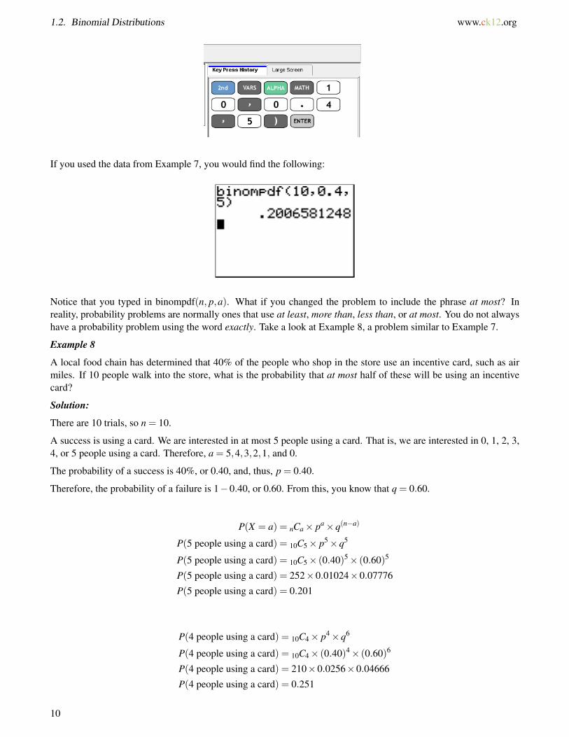
1.2. Binomial Distributions www.ck12.org
If you used the data from Example 7, you would find the following:
Notice that you typed in binompdf(n, p,a). What if you changed the problem to include the phrase at most? Inreality, probability problems are normally ones that use at least, more than, less than, or at most. You do not alwayshave a probability problem using the word exactly. Take a look at Example 8, a problem similar to Example 7.
Example 8
A local food chain has determined that 40% of the people who shop in the store use an incentive card, such as airmiles. If 10 people walk into the store, what is the probability that at most half of these will be using an incentivecard?
Solution:
There are 10 trials, so n = 10.
A success is using a card. We are interested in at most 5 people using a card. That is, we are interested in 0, 1, 2, 3,4, or 5 people using a card. Therefore, a = 5,4,3,2,1, and 0.
The probability of a success is 40%, or 0.40, and, thus, p = 0.40.
Therefore, the probability of a failure is 1−0.40, or 0.60. From this, you know that q = 0.60.
P(X = a) = nCa × pa ×q(n−a)
P(5 people using a card) = 10C5 × p5 ×q5
P(5 people using a card) = 10C5 × (0.40)5 × (0.60)5
P(5 people using a card) = 252×0.01024×0.07776
P(5 people using a card) = 0.201
P(4 people using a card) = 10C4 × p4 ×q6
P(4 people using a card) = 10C4 × (0.40)4 × (0.60)6
P(4 people using a card) = 210×0.0256×0.04666
P(4 people using a card) = 0.251
10

www.ck12.org Chapter 1. Probability Distributions
P(3 people using a card) = 10C3 × p3 ×q7
P(3 people using a card) = 10C3 × (0.40)3 × (0.60)7
P(3 people using a card) = 120×0.064×0.02799
P(3 people using a card) = 0.215
P(2 people using a card) = 10C2 × p2 ×q8
P(2 people using a card) = 10C2 × (0.40)2 × (0.60)8
P(2 people using a card) = 45×0.16×0.01680
P(2 people using a card) = 0.121
P(1 person using a card) = 10C1 × p1 ×q9
P(1 person using a card) = 10C1 × (0.40)1 × (0.60)9
P(1 person using a card) = 10×0.40×0.01008
P(1 person using a card) = 0.0403
P(0 people using a card) = 10C0 × p0 ×q10
P(0 people using a card) = 10C0 × (0.40)0 × (0.60)10
P(0 people using a card) = 1×1×0.00605
P(0 people using a card) = 0.00605
The total probability for this example is calculated as follows:
P(X ≤ 5) = 0.201+0.251+0.215+0.121+0.0403+0.0605
P(X ≤ 5) = 0.834
Therefore, the probability of seeing at most 5 people using a card in a random set of 10 people is 82.8%.
Technology Note
You can see now that the use of the TI-84 calculator can save a great deal of time when solving problems involvingthe phrases at least, more than, less than, or at most. This is due to the fact that the calculations become much morecumbersome. You could have used the binomcdf function on the TI-84 calculator to solve Example 8. Binomcdfstands for binomial cumulative probability. Binompdf simply stands for binomial probability.
The key sequence for using the binompdf function is as follows:
11

1.2. Binomial Distributions www.ck12.org
If you used the data from Example 8, you would find the following:
You can see how using the binomcdf function is a lot easier than actually calculating 6 probabilities and adding themup. If you were to round 0.8337613824 to 3 decimal places, you would get 0.834, which is our calculated valuefound in Example 8.
Example 9
Karen and Danny want to have 5 children after they get married. What is the probability that they will have exactly3 girls?
Solution:
There are 5 trials, so n = 5.
A success is when a girl is born, and we are interested in 3 girls. Therefore, a = 3.
The probability of a success is 50%, or 0.50, and thus, p = 0.50.
Therefore, the probability of a failure is 1−0.50, or 0.50. From this, you know that q = 0.50.
P(X = a) = nCa × pa ×q(n−a)
P(3 girls) = 5C3 × p3 ×q2
P(3 girls) = 5C3 × (0.50)3 × (0.50)2
P(3 girls) = 10×0.125×0.25
P(3 girls) = 0.3125
Therefore, the probability of having exactly 3 girls from the 5 children is 31.3%.
When using technology, you will select the binompdf function, because you are looking for the probability of exactly3 girls from the 5 children.
Using the TI-84 calculator gave us the same result as our calculation (and was a great deal quicker).
Example 10
12
www.ck12.org Chapter 1. Probability Distributions
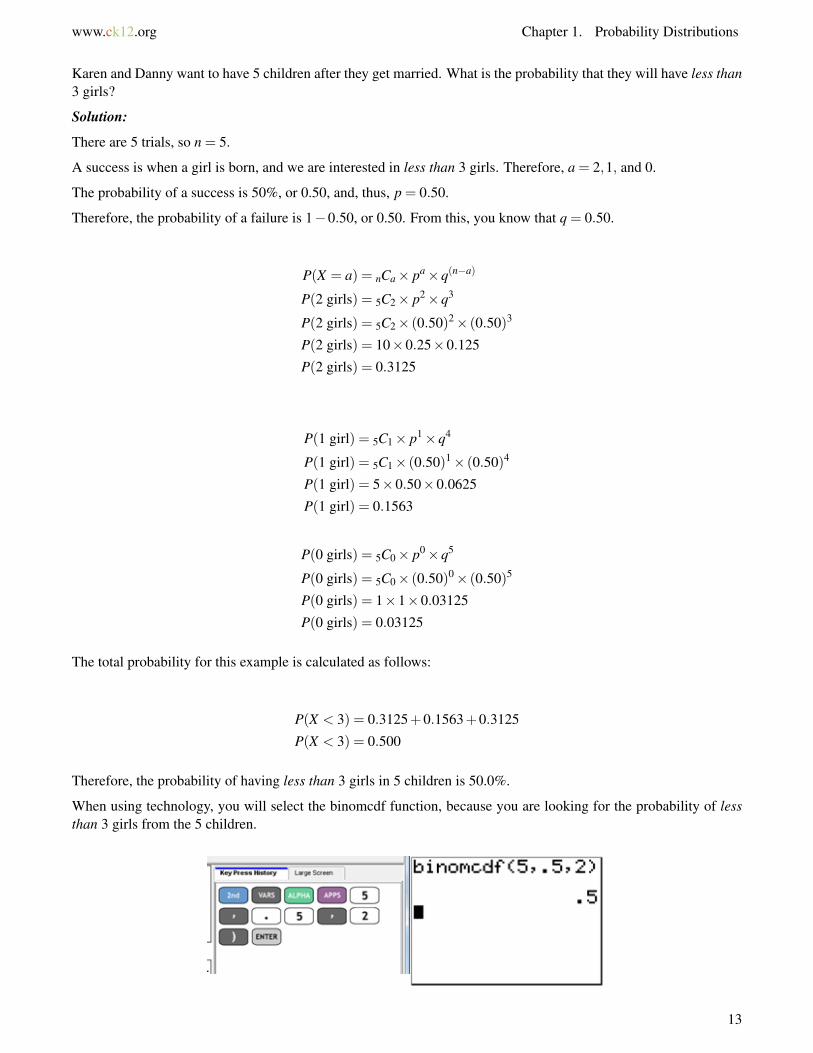
Karen and Danny want to have 5 children after they get married. What is the probability that they will have less than3 girls?
Solution:
There are 5 trials, so n = 5.
A success is when a girl is born, and we are interested in less than 3 girls. Therefore, a = 2,1, and 0.
The probability of a success is 50%, or 0.50, and, thus, p = 0.50.
Therefore, the probability of a failure is 1−0.50, or 0.50. From this, you know that q = 0.50.
P(X = a) = nCa × pa ×q(n−a)
P(2 girls) = 5C2 × p2 ×q3
P(2 girls) = 5C2 × (0.50)2 × (0.50)3
P(2 girls) = 10×0.25×0.125
P(2 girls) = 0.3125
P(1 girl) = 5C1 × p1 ×q4
P(1 girl) = 5C1 × (0.50)1 × (0.50)4
P(1 girl) = 5×0.50×0.0625
P(1 girl) = 0.1563
P(0 girls) = 5C0 × p0 ×q5
P(0 girls) = 5C0 × (0.50)0 × (0.50)5
P(0 girls) = 1×1×0.03125
P(0 girls) = 0.03125
The total probability for this example is calculated as follows:
P(X < 3) = 0.3125+0.1563+0.3125
P(X < 3) = 0.500
Therefore, the probability of having less than 3 girls in 5 children is 50.0%.
When using technology, you will select the binomcdf function, because you are looking for the probability of lessthan 3 girls from the 5 children.
13

1.2. Binomial Distributions www.ck12.org
Example 11
A fair coin is tossed 50 times. What is the probability that you will get heads in 30 of these tosses?
Solution:
There are 50 trials, so n = 50.
A success is getting a head, and we are interested in exactly 30 heads. Therefore, a = 30.
The probability of a success is 50%, or 0.50, and, thus, p = 0.50.
Therefore, the probability of a failure is 1−0.50, or 0.50. From this, you know that q = 0.50.
P(X = a) = nCa × pa ×q(n−a)
P(30 heads) = 50C30 × p30 ×q20
P(30 heads) = 50C30 × (0.50)30 × (0.50)20
P(30 heads) = (4.713×1013)× (9.313×10−10)× (9.537×10−7)
P(30 heads) = 0.0419
Therefore, the probability of getting exactly 30 heads from 50 tosses of a fair coin is 4.2%.
Using technology to check, you get the following:
Example 12
A fair coin is tossed 50 times. What is the probability that you will get heads in at most 30 of these tosses?
Solution:
There are 50 trials, so n = 50.
A success is getting a head, and we are interested in at most 30 heads. Therefore, a= 30,29,28,27,26,25,24,23,22,21,20,19,18,17,16,15,14,13,12,11,10,9,8,7,6,5,4,3,2,1,and, 0.
The probability of a success is 50%, or 0.50, and, thus, p = 0.50.
Therefore, the probability of a failure is 1−0.50, or 0.50. From this, you know that q = 0.50.
Obviously, you will be using technology to solve this problem, as it would take us a long time to calculate all of theindividual probabilities. The binomcdf function can be used as follows:
14

www.ck12.org Chapter 1. Probability Distributions
Therefore, the probability of having at most 30 heads from 50 tosses of a fair coin is 94.1%.
Example 13
A fair coin is tossed 50 times. What is the probability that you will get heads in at least 30 of these tosses?
Solution:
There are 50 trials, so n = 50.
A success is getting a head, and we are interested in at least 30 heads. Therefore, a= 50,49,48,47,46,45,44,43,42,41,40,39,38,37,36,35,34,33,32,31,and 30.
The probability of a success is 50%, or 0.50, and, thus, p = 0.50.
Therefore, the probability of a failure is 1−0.50, or 0.50. From this, you know that q = 0.50.
Again, you will obviously be using technology to solve this problem, as it would take us a long time to calculate allof the individual probabilities. The binomcdf function can be used as follows:
Notice that when you use the phrase at least, you used the numbers 50, 0.5, 29. In other words, you would type in 1− binomcdf (n, p,a−1). Since a = 30, at least a would be anything greater than 29. Therefore, the probability ofhaving at least 30 heads from 50 tosses of a fair coin is 10.1%.
Example 14
You have a summer job at a jelly bean factory as a quality control clerk. Your job is to ensure that the jelly beanscoming through the line are the right size and shape. If 90% of the jelly beans you see are the right size and shape,you give your thumbs up, and the shipment goes through to processing and on to the next phase to shipment. Anormal day at the jelly bean factory means 15 shipments are produced. What is the probability that exactly 10 willpass inspection?
Solution:
There are 15 shipments, so n = 15.
A success is a shipment passing inspection, and we are interested in exactly 10 passing inspection.
Therefore, a = 10.
The probability of a success is 90%, or 0.90, and, thus, p = 0.90.
Therefore, the probability of a failure is 1−0.90, or 0.10. From this, you know that q = 0.10.
15

1.2. Binomial Distributions www.ck12.org
P(X = a) = nCa × pa ×q(n−a)
P(10 shipments passing) = 15C10 × p10 ×q5
P(10 shipments passing) = 15C10 × (0.90)10 × (0.10)5
P(10 shipments passing) = 3003×0.3487× (1.00×10−5)
P(10 shipments passing) = 0.0105
Therefore, the probability that exactly 10 of the 15 shipments will pass inspection is 1.05%.
16

www.ck12.org Chapter 1. Probability Distributions
1.3 Exponential Distributions
A third type of probability distribution is an exponential distribution. When we discussed normal distributions, orstandard distributions, we talked about the fact that these distributions used continuous data, so you could usestandard distributions when talking about heights, ages, lengths, temperatures, and the like. The same types of dataare used when discussing exponential distributions. Exponential distributions, contrary to standard distributions,deal more with rates or changes over time. For example, the length of time the battery in your car will last is anexponential distribution. The length of time is a continuous random variable. A continuous random variable isone that can form an infinite number of groupings. So time, for example, can be broken down into hours, minutes,seconds, milliseconds, and so on. Another example of an exponential distribution is the lifetime of a computer part.Different computer parts have different life spans, depending on their use (and abuse). The rate of decay of thecomputer part determines the shape of the exponential distribution.
Let’s look at the differences between the normal distribution curve, a binomial distribution histogram, and anexponential distribution. List some of the similarities and differences that you see in the figures below.
Notice that with the standard distribution and the exponential distribution curves, the data represents continuousvariables. The data in the binomial distribution histogram, on the other hand, is discrete. Also, the curve for the
17

1.3. Exponential Distributions www.ck12.org
standard distribution is symmetrical about the mean. In other words, if you draw a horizontal line through the centerof the curve, the 2 halves of the standard distribution curve would be mirror images of each other. This symmetrydoes not exist for the exponential distribution curve (nor for the binomial distribution). Did you notice anythingelse?
Let’s look at some examples where the resulting graphs would show you an exponential distribution.
Example 15
ABC Computer Company is doing a quality control check on their newest core chip. They randomly chose 25 chipsfrom a batch of 200 to test and examined them to see how long they would continuously run before failing. Thefollowing results were obtained:
TABLE 1.3:
Number of Chips Hours to Failure8 1,0006 2,0004 3,0003 4,0002 5,0002 6,000
What kind of data is represented in the table?
Solution:
In order to solve this problem, you need to graph it to see what it looks like. You can use graph paper or yourcalculator. Entering the data into the TI-84 involves the following keystrokes. There are a number of them, becauseyou have to enter the data into L1 and L2, and then plot the lists using STAT PLOT.
After you press GRAPH , you get the following curve.
18

www.ck12.org Chapter 1. Probability Distributions
This curve looks somewhat like an exponential distribution curve, but let’s test it out. You can do this on the TI-84by pressing STAT , going to the CALC menu, pressing 0 , and pressing ENTER .
Notice that the r2 value is close to 1. This value indicates that an exponential curve is a good fit for this data and thatthe data, therefore, represents an exponential distribution.
You use regression to determine a rule that best explains the data you are observing. There is a standard quantitativemeasure of this best fit, known as the coefficient of determination (r2). The value of r2 can be from 0 to 1, and thecloser the value is to 1, the better the fit. In our data above, the r2 value is 0.9856 for the exponential regression. Ifwe had done a quadratic regression instead of an exponential regression, our r2 value would have been 0.9622. Thedata is not linear, but if we thought it might be, the r2 value would have been 0.9161. Remember, the higher the r2
value, the better the fit.
You can even go 1 step further and graph the exponential regression curve on top of our plotted points. Follow thekeystrokes below and test it out.
Note: It was not indicated that the data was in L1 and L2 when finding the exponential regression. This is becauseit is the default of the calculator. If you had used L2 and L3, you would have had to add this to your keystrokes.
19

1.3. Exponential Distributions www.ck12.org
Take a look at the formula that you used with the exponential regression calculation (ExpReg) above. The generalformula was y = abx. This is the characteristic formula for an exponential distribution curve. Siméon Poisson wasone of the first to study exponential distributions with his work in applied mathematics. The Poisson distribution, asit is known, is a form of an exponential distribution. He received little credit for his discovery during his lifetime, asit only found application in the early part of the 20th century, almost 70 years after Poisson had died. To read moreabout Siméon Poisson, go to http://en.wikipedia.org/wiki/Sim%C3%A9on_Denis_Poisson.
Example 16
Radioactive substances are measured using a Geiger-Müller counter (or a Geiger counter for short). Robert wasworking in his lab measuring the count rate of a radioactive particle. He obtained the following data:
TABLE 1.4:
Time (hr) Count (atoms)15 54412 2729 1366 683 341 17
20

www.ck12.org Chapter 1. Probability Distributions
Is this data representative of an exponential distribution? If so, find the equation. What would be the count at 7.5hours?
Solution:
Remember, we can plot this data using pencil and paper, or we can use a graphing calculator. We will use a graphingcalculator here.
The resulting graph appears as follows:
At a glance, it does look like an exponential curve, but we really have to take a closer look by doing the exponentialregression.
21

1.3. Exponential Distributions www.ck12.org
In the analysis of the exponential regression, we see that the r2 value is close to 1, and, therefore, the curve is indeedan exponential curve. We should go 1 step further and graph this exponential equation onto our coordinate grid andsee how close a match it is.
It is a very good match, so the equation representing our data is, therefore, y = 15.06(1.274x).
The last part of our problem asked us to determine what the count was after 7.5 hours. In other words, what is ywhen x = 7.5? This question can be answered as shown below:
y = 15.06(1.274x)
y = 15.06(1.2747.5)
y = 15.06(6.149)
y = 92.6 atoms
We can check this on our calculator as follows:
Our calculation is a bit over, because we rounded the values for a and b in the equation y = abx, whereas thecalculator did not.
Example 17
Jack believes that the concentration of gold decreases exponentially as you move further and further away from themain body of ore. He collects the following data to test out his theory:
22

www.ck12.org Chapter 1. Probability Distributions
TABLE 1.5:
Distance (m) Concentration (g/t)0 320400 80800 201,200 51,600 1.252,000 0.32
Is this data representative of an exponential distribution? If so, find the equation. What is the concentration at 1,000m?
Solution:
Again, we can plot this data using pencil and paper, or we can use a graphing calculator. As with Example 16, wewill use a graphing calculator here.
The resulting graph appears as follows:
23

1.3. Exponential Distributions www.ck12.org
At a glance, it does look like an exponential curve, but we really have to take a closer look by doing the exponentialregression.
In the analysis of the exponential regression, we see that the r2 value is close to 1, and, therefore, the curve is indeedan exponential curve. We will go 1 step further and graph this exponential equation onto our coordinate grid and seehow close a match it is.
It is a very good match, so the equation representing our data is, therefore, y = 318.56(0.9965x).
The problem asks, “What is the concentration at 1,000 m?” This question can be answered as shown below:
y = 318.56(0.9965x)
y = 318.56(0.99651000)
y = 318.56(0.03001)
y = 9.56 g/t
Therefore, the concentration of gold is 9.56 grams of gold per ton of rock.
We can check this on our calculator as follows:
Our calculation is a bit under, because we rounded the values for a and b in the equation y = abx, whereas thecalculator did not.
Points to Consider
24
www.ck12.org Chapter 1. Probability Distributions
• Why is a normal distribution considered to be a continuous probability distribution, whereas a binomialdistribution is considered to be a discrete probability distribution?
• How can you tell if a curve is truly an exponential distribution curve?
Vocabulary
Binomial experimentsExperiments that include only 2 choices, with distributions that involve a discrete number of trials of these 2
possible outcomes.
Binomial distributionA probability distribution of the successful trials of a binomial experiment.
Continuous random variableA variable that can form an infinite number of groupings.
Continuous variablesVariables that take on any value within the limits of the variable.
Continuous dataData where an infinite number of values exist between any 2 other values. Data points are joined on a graph.
Coefficient of determination (r2)A standard quantitative measure of best fit. Has values from 0 to 1, and the closer the value is to 1, the better the fit.
Discrete valuesData where a finite number of values exist between any 2 other values. Data points are not joined on a graph.
DistributionThe description of the possible values of a random variable and the possible occurrences of these values.
Exponential distributionA probability distribution showing a relation in the form y = abx.
Normal distribution curveA symmetrical curve that shows the highest frequency in the center (i.e., at the mean of the values in the distribution)
with an identical curve on either side of that center.
Standard distributionsNormal distributions, which are often referred to as bell curves.
25

1.4. Review Questions www.ck12.org
1.4 Review Questions
Answer the following questions and show all work (including diagrams) to create a complete answer.
1. Look at the following graphs and indicate whether they are binomial distributions, normal (standard) distribu-tions, or exponential distributions. Explain how you know.
a.
b.
c.
d.
2. Look at the following graphs and indicate whether they are binomial distributions, normal (standard) distribu-tions, or exponential distributions. Explain how you know.
a.
26

www.ck12.org Chapter 1. Probability Distributions
b.
c.
d.
3. It is determined that because of a particular genetic trend in a family, the probability of having a boy is 60%.Janet and David decide to have 4 children. What is the probability that they will have exactly 2 boys?
4. For question 3, what is the probability that Janet and David will have at least 2 boys?
5. For question 3, what is the probability that Janet and David will have at most 2 boys?6. The following data was collected on a recent 25-point math quiz. Does the data represent a normal distribu-
tion? Can you determine anything from the data?
20 17 22 23 25
14 15 14 17 9
18 2 11 18 19
14 21 19 20 18
16 13 14 10 12
7. A recent blockbuster movie was rated PG, with an additional violence warning. The manager of a movietheater did a survey of moviegoers to see what ages were attending the movie in an attempt to see if peoplewere adhering to the warnings. Is his data normally distributed? Do moviegoers at the theater regularly adhere
27

1.4. Review Questions www.ck12.org
to warnings?
17 9 20 27 16
15 14 24 19 14
19 7 21 18 12
5 10 15 23 14
17 13 13 12 14
8. The heights of coniferous trees were measured in a local park in a regular inspection. Is the data normallydistributed? Are there areas of the park that seem to be in danger? The measurements are all in feet.
22.8 9.7 23.2 21.2 23.5
18.2 7.0 8.8 25.7 19.4
25.0 8.8 23.0 23.2 20.1
23.1 18.5 21.7 21.7 9.1
4.3 7.8 3.4 20.0 8.5
9. Thomas is studying for his AP Biology final. In order to complete his course, he must do a self-directedproject. He decides to swab a tabletop in the student lounge and test for bacteria growing on the surface.Every hour, he looks in his Petri dish and makes an estimate of the number of bacteria present. The followingresults were recorded.
TABLE 1.6:
Time (hr) Bacteria Count0 11 62 403 2154 1,3005 7,800
28

www.ck12.org Chapter 1. Probability Distributions
Is this data representative of an exponential distribution? If so, find the equation. What is the count after 1 day?
10. If you watch a grasshopper jump, you will notice the following trend:
TABLE 1.7:
Jump Number Distance (m)1 42 23 1.14 0.515 0.256 0.13
Is this data representative of an exponential distribution? If so, find the equation. Why do you think the grasshopper’sdistance decreased with each jump?
29