Embed Size (px)
Citation preview

BR
EA
ST
CA
NC
ER
HIS
TO
PA
TH
OL
OG
ICA
L IM
AG
E
CL
AS
SIF
ICA
TIO
N U
SIN
G N
EU
RA
L N
ET
WO
RK
S
NU
RD
EE
N N
AT
FA
N
EU
2017
BREAST CANCER HISTOPATHOLOGICAL IMAGE
CLASSIFICATION USING NEURAL NETWORK
A THESIS SUBMITTED TO THE GRADUATE
SCHOOL OF APPLIED SCIENCES
OF
NEAR EAST UNIVERSITY
By
NURDEEN NATFA
In Partial Fulfilment of the Requirements for
the Degree of Master of Science
in
Electrical and Electronic Engineering
NICOSIA, 2017

I hereby declare that all information in this document has been obtained and presented in
accordance with academic rules and ethical conduct. I also declare that, as required by these
rules and conduct, I have fully cited and referenced all material and results that are not original
to this work.
Name, Last name: NURDEEN NATFA
Signature:
Date:

i
ACKNOWLEDGMENTS
I would like to express my deepest thanks and sincere appreciation to my supervisor in this
work, Assistant Prof. Dr. Kamil DIMILILER; who was my motivator during the work of this
modest thesis. It is time to thank him for all his patience and guidance throughout all my study
for my master degree. Prof. Dimililer’s knowledge and critics were very important to put me
on the right way and to enlighten my ideas and inspired me with new thinking manner. My
deepest gratefulness is expressed also to all my family members, and my wife who was my
great fan and supporter. I will always be grateful to my dear friends, colleagues, and the
Libyan community in the TRNC.

ii
To my parents and family….

iii
ABSTRACT
Breast cancer is one of the most famous types of cancer that affect the women during the last
decades. According to medical statistics, 12.6% of women around the world are subject to this
type of cancer. The disease is very dangerous and causes the death of a lot of women.
However, it is medically possible to treat it totally if it is detected in its early stages. The early
detection of breast cancer is one of the most important cure systems that can save the lives of
millions of women around the world. Periodic check is one of the main methods of detection
of the breast cancer. However, the lack of experience of many women and the lack of
specialized medical centres in many areas around the world makes it difficult to be achieved
completely. Artificial Neural Networks are very famous for their huge capabilities to simulate
the human brain. They have been used in many medical fields for disease detection and
classification. They are also implemented in different medical instruments to help medical
experts to identify the diseases. The use of ANN structures for the early detection of breast
cancer is one of the promising projects to save lives of women around the world. This work
will concentrate on the implementation of ANN for the detection of infected tissue of the
breast with breast cancer. Database of the disease images will be collected throughout this
work, processed, and used with artificial neural network. Practical results will be collected,
printed, and discussed as well.
Keywords: Artificial networks; back propagation; breast cancer; malignant tumor; benign
tumor

iv
ÖZET
Son yüzyılda, kadınları etkileyen en çok bilinen kanser türlerinden biri göğüs kanseridir. Tıp
statistiklerine göre, dünya kadınlarının % 12.6’sı bu kanser türünden muzdariptirler. Hastalık
tehlikeli ve de bir çok kadın için ölümcüldür. Erken tanı sayesinde tam tedavi edilebilir. Göğüs
kanserinin erken teşhisi, milyonlarca kadının hayatını kurtaracak en önemli safhadır. Göğüs
kanserinin teşhisinde periodik kontroller en temel yollardan birisidir. Fakat, bir çok kadının bu
konuda deneyimsiz oluşu ve dünyanın bir çok yerinde olmayan uzman tıp merkezleri
nedeniyle bu konuda hedefe varmakta zorluklar olmaktadır. Yapay Sinir Ağları insan beynini
simule etme konusunda çok büyük bir yeteneğe sahiptirler. Hastalıkların belirlenmesinde ve
sınıflandırılmasında bir çok tıp merkezlerinde kullanılmaktadirlar. Ayrıca, tıp uzmanlarının
hastalığı teşhisinde değişik tıbbı aletlerde de uygulanmaktadır. Göğüs kanserinin erken
teşhisinde ANN, kadınların hayatlarını kurtarma konusunda yapılan ve ümit vadeden
projelerden birisidir. Bu çalışma, ANN’in daha fazla, göğüsteki bakterili dokuyu ve göğüs
kanserinin teşhisinde kullanılmasına ağırlık verecektir.
Anahtar Kelimeler: Yapay sinir ağları; geri yayılım; göğüs kanseri; büyüyen tümör; kötü
huylu tümör

v
TABLE OF CONTENTS
ACKNOWLEDGMENTS .......................................................................................................... i
ABSTRACT ............................................................................................................................. iii
ÖZET ......................................................................................................................................... iv
TABLE OF CONTENTS .......................................................................................................... v
LIST OF TABLES .................................................................................................................. vii
LIST OF FIGURES ............................................................................................................... viii
LIST OF ABBREVIATIONS ................................................................................................... x
CHAPTER 1 : INTRODUCTION
1.1 Introduction ....................................................................................................................... 1
1.2 Literature Review .............................................................................................................. 2
1.3 Methodology of the Work ................................................................................................. 3
CHAPTER 2 : IMAGE PROCESSING TECHNIQUES
2.1 Introduction ....................................................................................................................... 6
2.2 Human Visual System ....................................................................................................... 6
2.3 Image and Image Representation ...................................................................................... 7
2.3.1 Binary Images ............................................................................................................. 8
2.3.2 Gray-scale Images ...................................................................................................... 9
2.3.3 Colour Images ............................................................................................................ 9
2.4 Image Processing .......................................................................................................... 10
2.4.1 Image segmentation .................................................................................................. 11
2.4.2 Filtering techniques .................................................................................................. 11
2.4.2.1 Wiener filter ................................................................................................... 12
2.5 Used Techniques in Our Work ........................................................................................ 13

vi
CHAPTER 3 : IMAGE PROCESSING TECHNIQUES
3.1 Introduction ..................................................................................................................... 19
3.2 Early Neural Networks .................................................................................................... 19
3.3 The Biological Neurons vs. Artificial Neurons ............................................................... 20
3.4 Artificial Neural Networks .............................................................................................. 22
3.4.1 Components of the Neural Networks ....................................................................... 23
3.4.2 Synaptic weights ....................................................................................................... 23
3.4.3 Layers ....................................................................................................................... 23
3.4.4 Summation functions ................................................................................................ 24
3.4.5 Activation function ................................................................................................... 24
3.4.6 Linear activation function ......................................................................................... 24
3.4.7 Sigmoid transfer function ......................................................................................... 26
3.5 Types of Neural Networks ............................................................................................... 27
3.5.1 Fully connected neural networks .............................................................................. 27
3.5.2 Partially connected neural networks ......................................................................... 28
3.5.3 Feed Forward Neural Network ................................................................................. 28
3.6 Back Propagation Learning Algorithm............................................................................ 29
CHAPTER 4: RESULTS AND DISCUSSIONS
4.1 Introduction ..................................................................................................................... 30
4.2 Image Processing Techniques ......................................................................................... 30
4.3 Back Propagation Artificial Neural Network .................................................................. 34
4.4 Two Step Learning Artificial Neural Network ................................................................ 39
CHAPTER 5: CONCLUSIONS
REFERENCES ........................................................................................................................ 44

vii
LIST OF TABLES
Table 4.1: Back propagation training parameters ..................................................................... 35
Table 4.2: Training output of first sample of images................................................................ 36
Table 4.3: Test output of first sample of images ...................................................................... 37
Table 1.1: Parameters of the second ANN experiment.............................................................37
Table 4.5: Training output of sample images ........................................................................... 38
Table 4.6: Test output of sample of images .............................................................................. 38
Table 4.7: Parameters of the two step learning ANN ............................................................... 39
Table 4.8: Comparison of back propagation algorithm results.................................................41

viii
LIST OF FIGURES
Figure 1.1: Sample of the mining tumor image. ......................................................................... 4
Figure 1.2: Sample of the malignant tumor image. .................................................................... 4
Figure 1.3: Flowchart of the proposed methods ......................................................................... 5
Figure 2.1: RGB image, gray image, and binary image of tissue ............................................... 8
Figure 2.2: HSL colour image space ........................................................................................ 10
Figure 2.3: Wiener filter for image restoration ............................................................... 13
Figure 2.4: Median filter for image filtering ............................................................................ 15
Figure 2.5: Execution of the image processing code ................................................................ 15
Figure 2.6: RGB image of the tissue before being processed................................................... 16
Figure 2.7: Gray scale image of the tumor tissue ..................................................................... 16
Figure 2.8: Gray scale level from zero to 255. ......................................................................... 16
Figure 2.9: Gray scale image after being filtered using Wiener filter ...................................... 17
Figure 2.10: Segmented image of the tissue ............................................................................. 17
Figure 2.11: Final Processed images of the tissue .................................................................... 18
Figure 3.1: Structure of the biological nervous cell ................................................................. 21
Figure 3.2: The synaptic connection between two neurons ...................................................... 21
Figure 3.3: Simple structure of the neural network .................................................................. 22
Figure 3.4: Linear activation function ...................................................................................... 25
Figure 3.5: Saturated linear activation function ....................................................................... 25
Figure 3.6: Sigmoid transfer function of ANN (logsig) ........................................................... 26
Figure 3.7: Sigmoid transfer function (tansig function) ........................................................... 26
Figure 3.8: Radial basis transfer function ................................................................................. 27
Figure 3.9: Totally connected neural network .......................................................................... 27
Figure 3.10: Partially connected neural networks .................................................................... 28
Figure 3.11: Feed forward artificial neural network structure .................................................. 28
Figure 3.12: Error back propagation algorithm ........................................................................ 29
Figure 4.1: Flow chart of the proposed work ........................................................................... 31
Figure 4.2: Original image of the tissue ................................................................................... 32
Figure 4.3: Converted gray scale image ................................................................................... 33

ix
Figure 4.4: Filtered image using median filter ......................................................................... 33
Figure 4.5: Small images fitted to ANN structure .................................................................... 34
Figure 4.6: Training tool of the artificial neural network ......................................................... 35
Figure 4.7: Training MSE evolution with time ........................................................................ 36
Figure 4.8: Curve of MSE during the training .......................................................................... 38
Figure 4.9: MSE curve of the pre-training network ................................................................. 40
Figure 4.10: MSE curve of the fine tuning stage of Two Step ANN ....................................... 40

x
LIST OF ABBREVIATIONS
ANN: Artificial Neural Network
CNN: Convolution Neural Networks
MSE: Mean Squared Error

1
1 CHAPTER 1
INTRODUCTION
1.1 Introduction
Cancer is a well known and spread public health problem around the world. According to
medical care agencies, in 2012 approximately 8.2 million death were caused by cancer. The
number is horribly increasing and expected to become 27 million by 2030 (Spanhol, Oliveira,
Petitjean, & Heutte, 2016). Breast cancer is one of the most mortal cancer type among women.
Most of the death caused by breast cancer is mainly due to the wrong or late evaluation of the
cancer. Early detection of breast cancer is the key factor for the protection and survival of a
woman who is affected by breast cancer (Singh, Surinder, & Dharmendra, 2016). Breast tumor
is screened nowadays using mammography and X-Rays screening. Microwave detection is
also being used for the detection of breast cancer tumor. Although a lot of researches are being
carried out yearly about the roots of the breast cancer, no evidences have been found revealing
the main causes of the disease (Ahmad, Isa, & Hussain, 2013).
Scientific and medical researches revealed that the early detection of the cancer tumors
increases significantly the hope of curing patients (Jayaraj, Sanjana, & Darshini, n.d.). The
treatment of the cancer is also based on the kind of symptoms that must be classified
accurately. The main and most important classification of the cancer is to decide whether the
tumor is benign or malignant. In the case of benign tumors, the treatment is used with smaller
amounts. This is mainly because the higher chances of patient survival. The malignant tumor
on the other hand is more concerned by the strong treatment without considering the side
effects (Tripathy, 2013). For this reason, the correct detection and classification of cancer type
is a very important issue that can save the lives of millions of women.
Mammography is one of the important and most famous early detection techniques for breast
cancer. Mammogram images are in general studied and analyzed carefully by specialists to
observe the disease in its early stages. Converging patterns of the tissue and vessels are

2
described using mammograms. Any deviation from these patterns in mammogram is viewed
carefully and considered as possible cancer tumor.
Machine learning is one of the most promising breast cancer detection techniques (Jayaraj et
al., n.d.). It can offer a potential support for medical doctors to evaluate faster and more
accurately the tumor type. The use of artificial intelligence and machine learning can offer a
very cheap, fast, easy, and accurate method for tumor kind detection. An intelligent system
provided with enough information can assist also medicines in the classification and
evaluation of the infection type.
Artificial neural networks are widely used nowadays in different science fields. They present a
powerful tool that can work and learn the same way human brains do. They have the potential
to generalize patterns and learn using examples. Development of digital processing
technologies is increasing the power of the artificial neural networks. Fast computers with
enough memories can perform very complex recognition and classification tasks in an
accurate and fast manner.
This work proposes the use of artificial neural networks in the classification of histo-
pathological breast images. The classification will be based on the type of cancer tumor in the
first stage into benign and malignant cancer. The next step will be used to find out the type of
the benign and malign cancer. For this reason, database of pathological images is collected and
going to be used with our system. The database is divided into two parts, benign and
malignant cancer. Each one of these is also divided into four sub divisions dependent on the
type of tumor. Images were collected using a microscope with different zooming settings.
1.2 Literature Review
The breast cancer has attracted the attention of medical doctors, laboratory specialists,
scientists, and image processing researchers. It is a common background of research for all
these specialists as its study requires the collaboration of them to obtain the best results. In
(Spanhol et al., 2016) the authors used 7909 histo-pathological images of breast cancer
acquired from 82 patients. This dataset contained malignant and benign images. The authors

3
presented a database called BreakHIS that represents a large amount of microscopic images
that is not easily present in public domain. A baseline pattern recognition system was then
proposed. In (A., S., Caroline, & Heutte, 2016) the same dataset was used with ANN for
breast cancer images classification. The dataset was divided arbitrarily into 70% for training
and 30% for test of the neural network efficiency. In the same work, SVM classification was
also applied and the results were compared with the ANN results. An artificial neural network
system for false alarm detection of in microwave breast cancer detectors was introduced in
(Singh et al., 2016). In this work a simple human breast model was built with a tumor of 5 mm
size to examine the microwave detection. In (Ahmad et al., 2013) a hybrid classifier composed
of genetic algorithm with artificial neural networks was proposed for the study of breast
cancer. The aim of the work was the improvement of the early detection systems of breast
cancer. The efficiency of the proposed method was reported to be 99.43% maximum and
98.29% average.
In (Pastrana-Palma, 2016), a study of the use of the ANN classification system with digital
mammographic images was presented. The obtained efficiency of the reported job was
approximately 80%. A pattern recognition approach for breast cancer detection and
classification was applied and presented in (Hassan, Mariam, Adnan, Gilles, & Leduc, 2016).
The pattern recognition in this work relied on the use of the well known artificial neural
networks. The work reported an accuracy of 99.3% of the training set. In (Jayaraj et al., n.d.),
the authors have presented a review of the breast cancer detection literature. Different works
were discussed and there accuracies were presented.
1.3 Methodology of the Work
In this work, the classification of the breast cancer images will pass by different steps. These
steps are subdivided into image processing and artificial neural classification. The first step
will concentrate on the reading of the different images and feature extraction of these images.
Processing of images will include the reading of the pnj images and converting them into gray
scale images for simplification of calculations. The gray images are then going to be filtered
using a suitable filtering method to extract the original pure image and reject the noise. After
filtering, images will be divided into two parts; the first for training and the other part will be
4
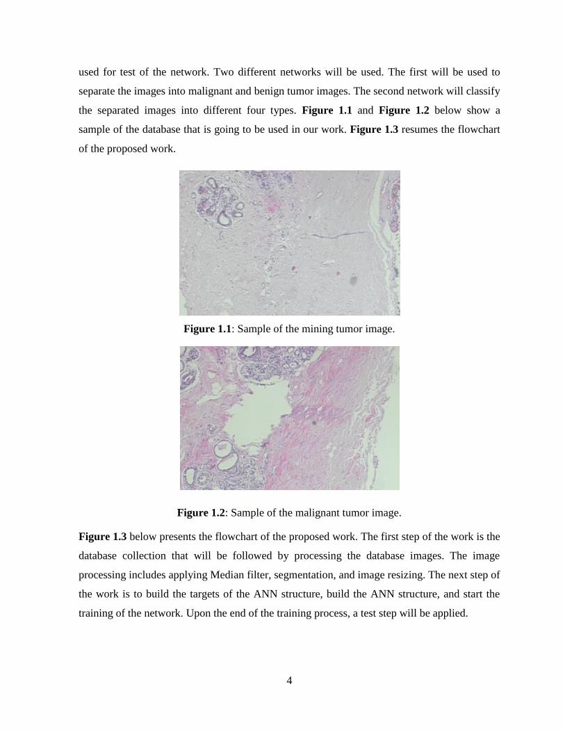
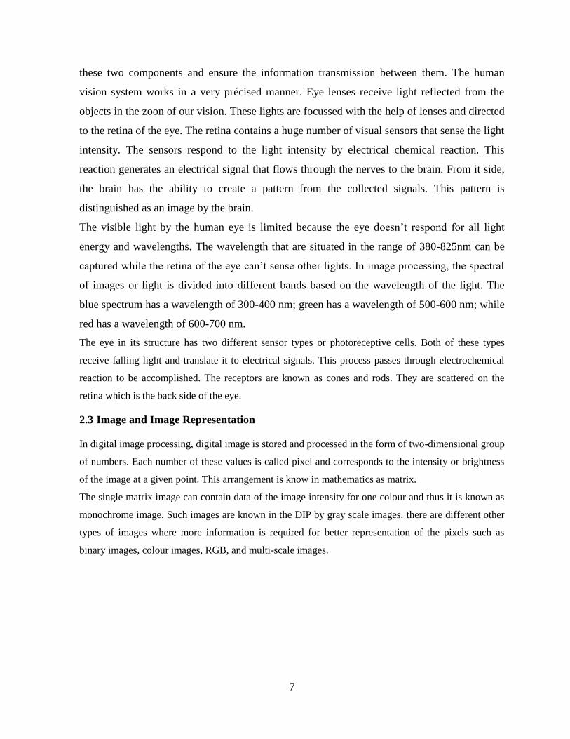
used for test of the network. Two different networks will be used. The first will be used to
separate the images into malignant and benign tumor images. The second network will classify
the separated images into different four types. Figure 1.1 and Figure 1.2 below show a
sample of the database that is going to be used in our work. Figure 1.3 resumes the flowchart
of the proposed work.
Figure 1.1: Sample of the mining tumor image.
Figure 1.2: Sample of the malignant tumor image.
Figure 1.3 below presents the flowchart of the proposed work. The first step of the work is the
database collection that will be followed by processing the database images. The image
processing includes applying Median filter, segmentation, and image resizing. The next step of
the work is to build the targets of the ANN structure, build the ANN structure, and start the
training of the network. Upon the end of the training process, a test step will be applied.

5
Read The images of Tumor
- normalize the images.Divide the images into different training and test sets
Vectorize the images
Build the target matrix for each set of images
Construct the suitable neural network
Start training of each set
MSE is OK?
Stop Training
print results
Yes
No
Apply Median filter on the images to remove noiseresize the image to an smaller size
Apply segmentation on the image and edge detection
averaging the image to extract features
Figure 1.3: Flowchart of the proposed methods

6
2 CHAPTER 2
IMAGE PROCESSING TECHNIQUES
2.1 Introduction
Computer images have become famous term in the sciences and public life. It opens the door
for connection with the external world by exchanging data through internet and computer
appliances. This process is a totally digital or can need the intervention of human being.
Computer vision term signifies that the process doesn’t need any human intervention. Thus the
whole process will be applied automatically by a digital processor and computers. Different
topics can be involved in the computer vision process such as image analysis. Image analysis
is another process that includes different subjects and extends for more wide research.
Image processing is a different subject that involves the human being touch in processing the
image. It has also many subjects involved, these topics include image restoration, image
enhancement, and many other processes. For better understanding of these different processes,
it is important to study the human vision system to generate a deep idea about its function and
properties. This chapter is intended for the study of human visual system and its main
characteristics. Different image processing techniques will also be treated in the course of this
chapter to build better idea about these techniques.
2.2 Human Visual System
Human visual system is something that we use unconsciously. Humans never think of the
effect of makeup on the physiological systems vision. It is important to discuss the
understanding of the process of distinguishing visual data. This discussion will allow for better
understanding of different methods implemented in image processing.
Human visual system is composed of two main interconnected parts; the eyes that are used for
capturing visual scenes and the brain that process the images, classify, and recognize them.
These two parts of the human visual system are connected between each other via nervous
links. The human eye is considered as a perfect imaging sensor with good resolution and
structure. The human brain is a super powerful processing system. Optic nerves are connecting
7
these two components and ensure the information transmission between them. The human
vision system works in a very précised manner. Eye lenses receive light reflected from the
objects in the zoon of our vision. These lights are focussed with the help of lenses and directed
to the retina of the eye. The retina contains a huge number of visual sensors that sense the light
intensity. The sensors respond to the light intensity by electrical chemical reaction. This
reaction generates an electrical signal that flows through the nerves to the brain. From it side,
the brain has the ability to create a pattern from the collected signals. This pattern is
distinguished as an image by the brain.
The visible light by the human eye is limited because the eye doesn’t respond for all light
energy and wavelengths. The wavelength that are situated in the range of 380-825nm can be
captured while the retina of the eye can’t sense other lights. In image processing, the spectral
of images or light is divided into different bands based on the wavelength of the light. The
blue spectrum has a wavelength of 300-400 nm; green has a wavelength of 500-600 nm; while
red has a wavelength of 600-700 nm.
The eye in its structure has two different sensor types or photoreceptive cells. Both of these types
receive falling light and translate it to electrical signals. This process passes through electrochemical
reaction to be accomplished. The receptors are known as cones and rods. They are scattered on the
retina which is the back side of the eye.
2.3 Image and Image Representation
In digital image processing, digital image is stored and processed in the form of two-dimensional group
of numbers. Each number of these values is called pixel and corresponds to the intensity or brightness
of the image at a given point. This arrangement is know in mathematics as matrix.
The single matrix image can contain data of the image intensity for one colour and thus it is known as
monochrome image. Such images are known in the DIP by gray scale images. there are different other
types of images where more information is required for better representation of the pixels such as
binary images, colour images, RGB, and multi-scale images.

8
Figure 2.1: RGB image, gray image, and binary image of tissue
2.3.1 Binary Images
Binary images can be considered as the most basic shape of images. From the name it can be
understood that they can take binary values of one or zero. Each pixel in the image is represented by a
one bit binary value. The colour can be either white or black. Binary images are known by 1 bit/pixel
rate for that reason. They are used in applications where the only required information is the shape
without details. They can be implemented in deformation inspection of products. The binary image is
normally generated by threshold process where the pixel value is considered true if it is more than a
given threshold and zero if it is less than that value.

9
2.3.2 Gray-Scale Images
These are the main example of monochrome images or single colour images. the pixels in the image
contains the brightness of the image only without any information about the spectral analysis of the
light. The brightness levels are function of the bit rate of the gray scale image. In an 8 bit image, there
are 256 different brightness levels. In a 16 bit image the number is raised up to 2552 different levels.
Typically, general images use 8 bit system and thus are represented by 256 levels of white and black
colours. This type of images is useful and easy for digital computers as it uses the byte in its pixel
representation which is the small standard unit in computers. In higher accuracy applications like
medical purpose images or astronomical images; high resolution of 12 or 16 bit/pixel can be
implemented. These high resolutions are useful in the zooming of the image. This process can show
details that couldn’t be seen with normal resolutions.
2.3.3 Colour Images
Coloured images are represented as multi band monochrome image information. In this
representation, each band of information matches with a unique colour. The real
information accumulated in the image is the level of the brightness of each colour or band.
In case the image is presented, the resultant brightness level is presented on the monitor
by picture pixels with the same intensity of the correspondent colour. Typically, colour
images are characterized in the form of R (red), G (green), and B (blue) colours. Using the
8 bit single colour paradigm, the destination colour image will have 24 bits in each single
pixel.
In many applications, RGB colour information is converted to another form of mathematical
model. In such models, the image is converted to one dimensional brightness matrix and
another two dimensional colour space. The last contains information about the relative
colour intensity rather than intensity.
HSL (hue, Saturation, Lightness) transform gives a description of colours in other way. The
hue is a description of how we see colour, the saturation is a measure of the white ration in
the colour, while brightness describes the intensity of light. This transform is actually built to
suit the human perception of colours. We can build a picture by describing the three values
of hue, saturation and brightness.

10
Figure 2.2: HSL colour image space
2.4 Image Processing
Image processing is the science of treating the images properties under the supervision of
human. After the treatment of the images, they should be controlled by humans to ensure it is
acceptable. To understand better the image processing techniques, understanding the human
visual system is a must. The main processes of image processing are image compression,
image enhancement, and image restoration.
Image restoration is known as the treatment of images that have some estimated or known
degree of degradation. These images are taken and restored to their initial state before
degradation. It is used in image photography or in fields of publications where image needs to
be visually perfect before being published. In such applications it is important to have an idea
about the type of degradation in order to be able to restore the image. This helps in creating a
model for the distortion in order to be able to apply its inverse on the image. The inverse
model of degradation will restore the distorted image to its initial and original state.

11
In the process of image enhancement, a normal image is processed to be improved even if it is
originally not distorted. This is done with help of the response of human visual system. A
simple and efficient enhancement method is the contrast stretching of the image.
Enhancement techniques are more likely to be problem oriented. This means that the method
that is used for satellite images enhancement can be unsuitable for medical images
enhancement. Despite the fact that enhancement and restoration are alike in purpose, to
ameliorate the vision of the image, they use different approaches to solve the problem. In
restoration, the process aims to model the distortion in order to inverse its effects. Whereas,
enhancement investigates in the human visual system experience to visually improve the
image quality.
The image compression is a totally different process in which the massive data of an image is
stored in smaller space of data. This is mainly achieved by eliminating visually unnecessary
data and make benefit of data redundancy in the image. Over more, computer applications and
digital vision systems doesn’t need every detail of the image. They can make better use of
compressed images.
2.4.1 Image Segmentation
Image segmentation is imperative in many applications. It is useful in different computer
assisted processes and image processing techniques. The segmentation of an image aims at
extracting the meaningful parts of an image and splitting the images into regions of interest
prior to the processes of higher levels. These processes include objects identification, image
classification. In reality, segmentation is very useful in finding any detail in an image.
Image segmentation techniques search for items that gain some amount of homogeneity or
have some match with their edges. Almost all segmentation techniques represent
modification, or combination of these two aspects. The measures of contrast and
homogeneity can include characteristics like level of gray, colour profile, or texture.
2.4.2 Filtering Techniques
Filtering is a procedure for image modification or enhancement that is implemented
used to highlight some features or to take rid of some other features. Image filtering is an

12
operation known by neighbourhood operation. Such operations indicate that the pixels value
is determined in function of the surrounding pixels. Special algorithms are applied on the
neighbouring pixels to evaluate the perfect value of the pixel. Some common filters are Sobel
filter, Laplacian of Gaussian, Unsharp filter, average filter, median filter, and wiener adaptive
filter. In this work, we are going to apply wiener adaptive filter for the enhancement of the
images.
2.4.2.1 Wiener Filter
Wiener filter is considered as one of the most important techniques in removing noise from
digital images. Wiener filter uses an estimation of the noise level in the noise removal process
(Frank, Floyd, Wilfredo, & Kincaid, 2014). Wienerr filter is able to work on noisy distorted
images better than any other filters. Wiener filter is defined by:
2
2*f
HW
H H k
(2.1)
Where H defines the fast Fourier transform of the noise model and k is a scalar
constant. After applying wiener filter on a noisy image, the filter removes the
noise from it and restores it to an original shape. Figure 2.3 below shows the
effect of adding noise to an image and removing the noise using wiener filter.

13
Figure 2.3: Wiener filter for image restoration
2.4.2.2 Median Filter
Median filter is implemented to decrease the noise levels in the images where there are
impulsive noise types. It creates clear image and less concentration in the image pixels. The
main idea in the median filter is to make rid of the strange pixels values within a window of
the image. Any strange value is eliminated by choosing the median value within the cluster of
pixels and fixing it in the centre; the cluster moves ahead and repeats the process until all
pixels are replaced by the median of their surrounding clusters.
The process of applying the median filter is very simple. A window around the required pixels
is defined and its statistical median value is found. This value is simply used as replacement of
that pixel value. The process continues replacing the pixels with their surrounding median
until all pixels are processed. This way; all pixels with values that are too far from their

14
neighbourhood are replaced with pixels that are similar. Figure 2.4 below presents the results
of image filtering using median filter. The figure shows how the median filter removes the
dots in the image.
Figure 2.4: Median filter for image filtering
In this work, different image processing techniques were used and applied on the images of
the tumor. The image processing phase included the next operations:
1- Reading the RGB images of the tumor.
2- Converting RGB images to Gray Scale images.
3- Applying Median filter to remove noise from images.
4- Segmenting the images by using the edge detection.
5- Resizing the image to reduce the data processed.
6- Converting the 2D image to 1D vector that can be fed to the neural network.
Original image
Noisy image
Median filtered image

15
7- Normalizing the pixel values of the image.
The image processing program was coded using MATLAB software in Figure 2.5 ; the figure
below presents the execution of the processing code during the image processing. The original
image of the tissue is presented in the Figure 2.5. This image contains information about
three colour spectrums. It is actually less useful for computerized processes. Figure 2.6
presents the gray scale image obtained from the previous image. It contains data about the
level of the gray colour in the form of 8 bit digital number. This level is presented on a scale
of 256 levels. The higher the gray level the whiter the image is. The level zero corresponds to
the black. Figure 2.7 presents the grades of gray level image.
Figure 2.5: Execution of the image processing code
The manipulation of gray scale images is easier and less memory consuming than the RGB
images with similar performance in computerized processes. The image matrix can be easily
processed in gray scale images. Most of filters can be applied on single colour images like
greyscale images. In our work, the Wiener filter was applied on the gray scale image to
remove any type of noise that can be contained in within. Figure 2.8 represents the filtered
image of the tissue. This image was segmented using zero crossing edge detection method.
The edges were detected and the resultant image is shown in Figure 2.10.

16
Figure 2.6: RGB image of the tissue before being processed
Figure 2.7: Gray scale image of the tumor tissue
Original Image of the tumor
Gray Scale Image
0 255

17
Figure 2.8: Gray scale level from zero to 255.
Figure 2.9: Gray scale image after being filtered using Wiener filter
Figure 2.10: Segmented image of the tissue
After detecting the edges and segmenting the image of the tumor tissue, this image is then
down scaled to reduce its size. The small size image is more suitable for the use with artificial
intelligence applications. All the details of the image can be contained in smaller version of
the image. Figure 2.11 above shows a sample of the small images of the tissue.
Wiener Filtered Image
Segmented Image

18
Figure 2.11: Final Processed images of the tissue

19
3 CHAPTER 3
ARTIFICIAL NEURAL NETWORKS
3.1 Introduction
Artificial neural networks are special structures designed for the imitation of the function of
biological nervous system. They have the ability to learn patterns based on different examples
and to model relations between different systems. This chapter will introduce the artificial
neural networks and discuss their basic structure.
3.2 Early Neural Networks
The idea of the neural networks has started early in the forties of the last century. A paper
entitled “A logical calculus in the ideas immanent in nervous activity” was published by two
scientists. These were Warren Mcculloch and Walter Pitts. The main idea in their published
paper was about the modelling of a system similar to the human nervous system. Their model
represented a mathematical model that was called later neuron. Their neuron had the ability to
receive and input and generate a suitable output (Colin, 1996).
The output from this simple neuron was a logical output that has one of two choices. It had the
ability to collect the inputs and decide whether they have enough power to activate an output
or not. When the received input reach certain level which is called threshold, the output is
activated; otherwise, the output is deactivated. More complex networks can be formed by
combining huge number of single cells of the same type. They will be activated or deactivated
the same way single neuron does. The theory created by pitts and Mcculloch was very
interesting and some types of networks are still named after their names.
The idea continued the same way during the 50s and 60s with small modifications. The
concept of perceptron was introduced in the field by the French psychologist Frank Rosenblatt
in the year 1958. The idea of perceptron was simple and made use of single neurons to create a
network. This network was interconnected to analyse data and information. Different
20
publications on the perceptron and neural networks were published until the beginning of 80s.
the main problem facing the perceptron was how to solve some complex types of relationship
s between input and output data (Cios & Shields, 1997).
In the year 1962, Rosenblatt was able to create a teaching process that guarantees the
convergence of the error function. His algorithm was an adjustment of the weights inside the
recognition loop during the teaching process. The process updates the values of the weights
until generating suitable outputs. The challenge for this system was mainly the slow and weak
computers of that time that were used just for very special applications and cost a lot of
money.
The cognition system was the early model of many layers networks. Such networks had a very
efficient learning process. The system construction, connections, and weights changed
between a structure and another. In 1982 Hopfield's networks were created and implemented
to propagate data in two directions(Minsky & Papert, 1969). The use of the back propagation
process for the learning of ANN was the main inspiration for the incorporation of the ANN in
the 80s. This process relies on the propagation of the error values through the different layers
of the neural networks. This error is used to evaluate the weight values and generate new
values for them. Since then, many different updating theories were proposed to guarantee the
minimization of the error signal after the weight updating process (Anderson & McNeill,
2010).
3.3 The Biological Neurons vs. Artificial Neurons
The brain is a huge computer composed of millions of millions of interrelated nerves. Each
one of these nerves is a biological cell in which different chemical and electrical processes are
happening endlessly. These processes are the main reason for the creation and transmission of
information and ideas. Each one of the nerves is connected to thousands of surrounding
neurons. At the moment any one of these neurons fires, an electrical signal arrives at the
dendrite. The entire received signals are collected and accumulated together. The
accumulation can occur in spatial or temporal domain. The total input received at the dendrite
is then transmitted to the soma of the cell. The role of the soma is to provide the required
maintenance for the cell parts. The nerve fires just if it’s received signal is enough and able to
21
fire. It is accepted that the output strength is constant whatever the strength of the input if it is
greater than the threshold. The output strength of output is also constant at all parts of the cell.
The synapses ensure the transmission of the signal from a neuron to the next neuron (Cios &
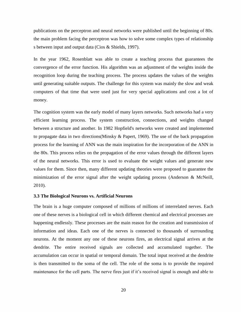
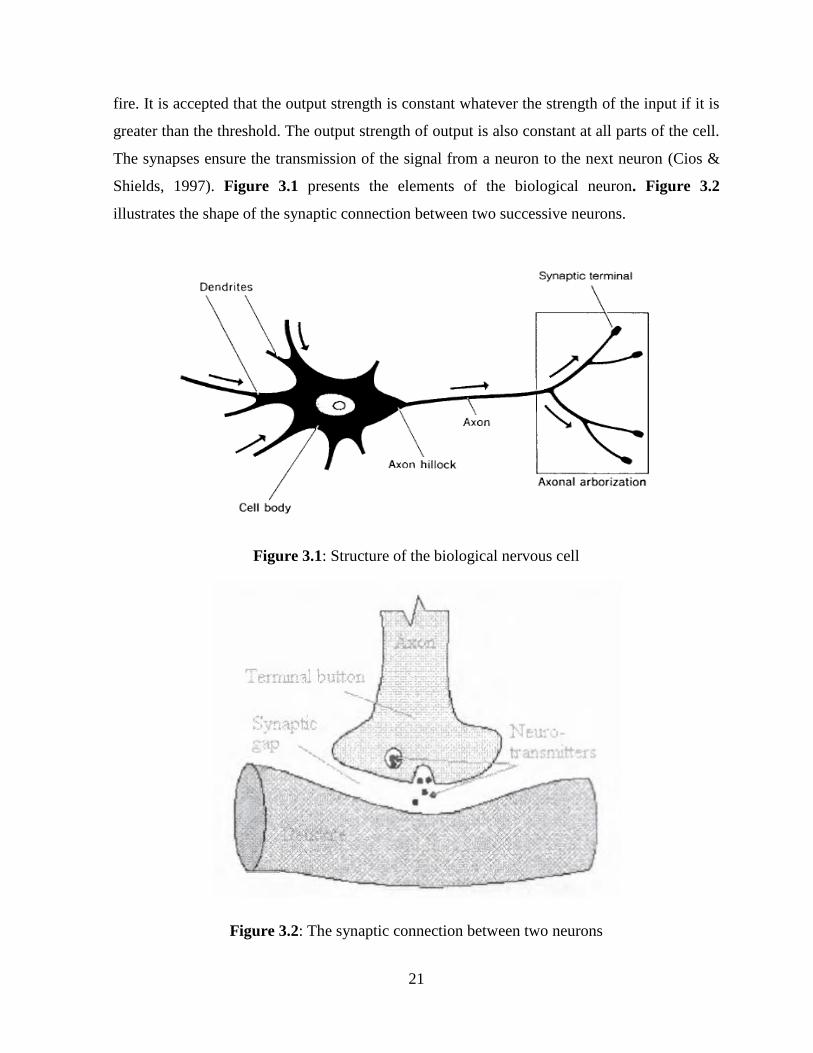
Shields, 1997). Figure 3.1 presents the elements of the biological neuron. Figure 3.2
illustrates the shape of the synaptic connection between two successive neurons.
Figure 3.1: Structure of the biological nervous cell
Figure 3.2: The synaptic connection between two neurons

22
3.4 Artificial Neural Networks
Neurobiologists have created sophisticated mathematical reproduction of biological neurons
That can be used in computers. Their model was very helpful in performing simulations of the
thinking process and to imitate the brain function. In electronics and computer sciences, the
interest is more consisted toward the uses and characteristics of such model. Simpler neurons
or neural models can be implemented in computer sciences as far as they present satisfactory
solutions for the different problems. While attempting to imitate the functions of the human
brain, scientists have built electronic circuits that had the ability to simulate the neural
networks. However, modern computers offer high flexibility in simulating the neural functions
and offering high performance artificial neural network (Colin, 1996).
The main element of a neural network is known as a node. The node receives its signals from
the other connected nodes or even from another source or sensor (Khashman & Dimililer,
2007). Every single input is connected to a related weight or factor. The weights can be
changed to simulate the learning in the synapses. Each unit has a function that is used to find
the sum of its inputs after being multiplied by the weights. The structure of the node is
presented in Figure 3.3. w
i1
wi2
wi3
∑ f
Out = f(net)
Figure 3.3: Simple structure of the neural network

23
The output of the node shown in the figure above can be given based on the next equation:
i iout x (2.2)
Where the x term denotes the inputs to the node and the omega denotes the associated weight
to each input.
3.4.1 Components of the Neural Networks
All types of artificial neural networks have the same components regardless of the position of
the neuron. The main components are explained below. These components include weights,
activation functions, summation elements, and scaling elements.
3.4.2 Synaptic weights
Artificial neuron receives many coincident signals from different sources. Each one of the
inputs has its own participation in the output of the system. The impact of each one of the
inputs is different from the other inputs. For this reason, each input is associated with a weight
or factor that manipulates the participation of the input in the summing output. Some inputs
are assigned more importance than others based on the training of the neurons. The greater the
weight assigned to the input, the greater the effect of the input on the result of the network.
Weights are adaptive factors inside the neural net. They decide the concentration of the
entering signal as recorded in the memory of the neural network. They can be considered as an
evaluation of the strength of the neuron input. These weights can be adjusted as a result of
multiple learning methods and dependent on the topology of the used network.
3.4.3 Layers
The layer in the neural network is a structure that contains different parts of the neural
networks inside it. Any neural network must have at least two layers in it; one for receiving
the inputs whiles the other is used to generate the outputs. Some structures of the neural
networks have multiple layers called hidden layers. Each layer contains inside it a number of
weights and summing functions.
24
3.4.4 Summation functions
Each structure of neural networks is constructed based on summing the inputs received at its
input and send the result to the output. Simply, the summation function is the function that
weights the inputs, find their sum, and send the result to another layer of structure. This
process is done through the use of scalar or vector product between the inputs of the neuron
and the weights of that neuron. Suppose having the inputs(x1, x2, ….xn) to a network that has
n weights (w1, w2, ….wn). the output generated frolm these inputs is given by:
i iout x (2.3)
3.4.5 Activation function
The output calculated in the summing function is generally passed through another operator
called transfer function. The transfer function decides the output of the neuron in term of
efficiency of the input. Transfer function takes the result of the summation and produces a
suitable output of it. In fact, there exit many shapes of transfer functions in artificial neural
networks. Ramps, hard limits, and sigmoid transfer functions are the main types of transfer
functions used in neural network applications.
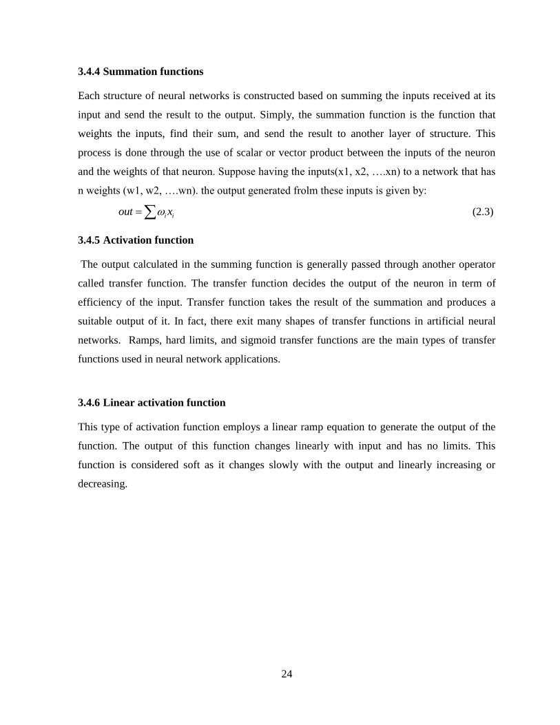
3.4.6 Linear activation function
This type of activation function employs a linear ramp equation to generate the output of the
function. The output of this function changes linearly with input and has no limits. This
function is considered soft as it changes slowly with the output and linearly increasing or
decreasing.
25
Figure 3.4: Linear activation function
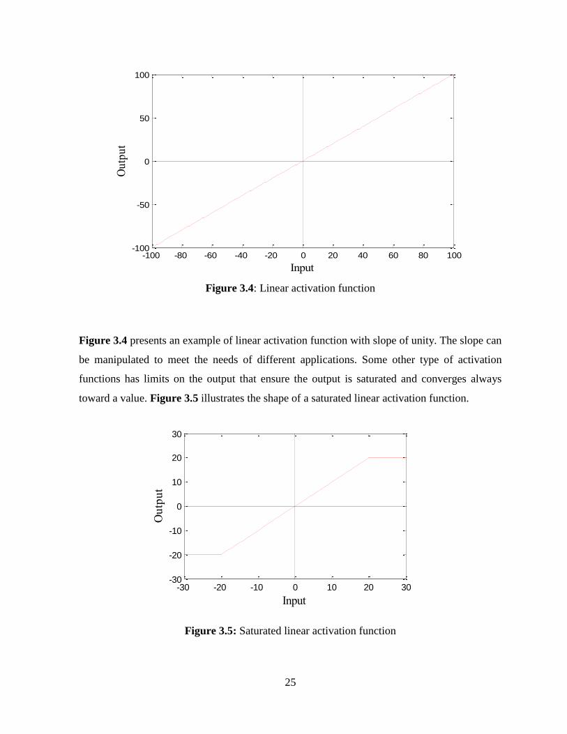
Figure 3.4 presents an example of linear activation function with slope of unity. The slope can
be manipulated to meet the needs of different applications. Some other type of activation
functions has limits on the output that ensure the output is saturated and converges always
toward a value. Figure 3.5 illustrates the shape of a saturated linear activation function.
Figure 3.5: Saturated linear activation function
-100 -80 -60 -40 -20 0 20 40 60 80 100-100
-50
0
50
100
Input
Ou
tpu
t
-30 -20 -10 0 10 20 30-30
-20
-10
0
10
20
30
Ou
tpu
t
Input

26
3.4.7 Sigmoid transfer function
Sigmoid is a mathematical function that is widely implemented in neural networks. The
sigmoid function is adaptable and can change based on the parameters used with it. It can be
used as linear limited function, hard limit function, or non linear function. There are two
different types of the sigmoid functions. These are the logarithmic and the tangential sigmoid
presented in Figure 3.6 and Figure 3.7 below.
Figure 3.6: Sigmoid transfer function of ANN (logsig)
Figure 3.7: Sigmoid transfer function (tansig function)
Figure 3.8 illustrates the use of another type of transfer functions which is the radial basis
transfer function. Its shape looks like a bell around the zero point. This transfer function also
can be used in ANN applications.
-100 -80 -60 -40 -20 0 20 40 60 80 100-2
-1
0
1
2
Input
Out
put
-100 -80 -60 -40 -20 0 20 40 60 80 100
-1
-0.5
0
0.5
1
Input
Ou
tpu
t

27
Figure 3.8: Radial basis transfer function
3.5 Types of Neural Networks
Neural networks layers are connected in between via different layers and connections. The
connections are in general unidirectional connections going from the input toward the output.
The input for a neuron can be single or multiple inputs. However, each neuron produces one
output. Neural networks can be classified according to the types of their connection into
different types.
3.5.1 Fully connected neural networks
In this type of neural network, each one of the neurons is connected to every single neuron of
the next and previous layer. Such type of connection is illustrated in the Figure 3.9.
Figure 3.9: Totally connected neural network
-10 -8 -6 -4 -2 0 2 4 6 8 100
0.5
1
Input
Ou
tpu
t

28
3.5.2 Partially connected neural networks
In this topology, each neuron is not forcedly connected with all neurons in the previous and
nex layer. Figure 3.10 shows this type of connection.
Figure 3.10: Partially connected neural networks
3.5.3 Feed Forward Neural Network
In this type of network, the signal moves in one direction from the input to the output. This
type can be either fully connected or partially connected. Figure 3.11 illustrates the
connection of this type of neural network. This type is considerably implemented in different
applications of the neural network. Generally, its name is connected to the back propagation
learning algorithm.
ww
ww
ww
ww
ww
ww
ww
ww
ww
ww
ww
ww
Input layerHidden
layers
Output
layer
Figure 3.11: Feed forward artificial neural network structure

29
3.6 Back Propagation Learning Algorithm
The back propagation has been one of the most efficient types of neural networks. It is widely
implemented in the training of the neural networks. Its name is derived from the fact that the
error signal is back propagated toward the input layer through the different layers. The process
of back propagation has two steps before being accomplished. The first step includes the
forward swap over the network where all inputs are weighted and passed through layers. The
generated output is then compared with a desired target to generate an error signal. The second
step includes the propagation of the error signal back to the previous layer. Then back to its
precedent until reaching the input layer. The weights of all layers are updated accordingly in
such a way that guarantees the error minimization.
The back propagation algorithm procedure continues in a repetitive mode until the resulting
error becomes small enough to generalize the network. Figure 3.12 illustrates the idea of
propagation of the error in the learning process of the network.
ww
ww
ww
ww
ww
ww
ww
ww
ww
ww
ww
ww
Input layerHidden
layers
Err
or c
alcu
latio
nE
rror
cal
cula
tion
Output
Error back
propagation
Figure 3.12: Error back propagation algorithm

30
4 CHAPTER 4
RESULTS AND DISCUSSIONS
4.1 Introduction
In this chapter, the implementation of the different image processing techniques along with the
back propagation artificial neural network will be presented. A new and efficient Two Step
learning artificial neural network structure will also be discussed and presented in the course o
this chapter. Results of the implementation will be discussed and presented.
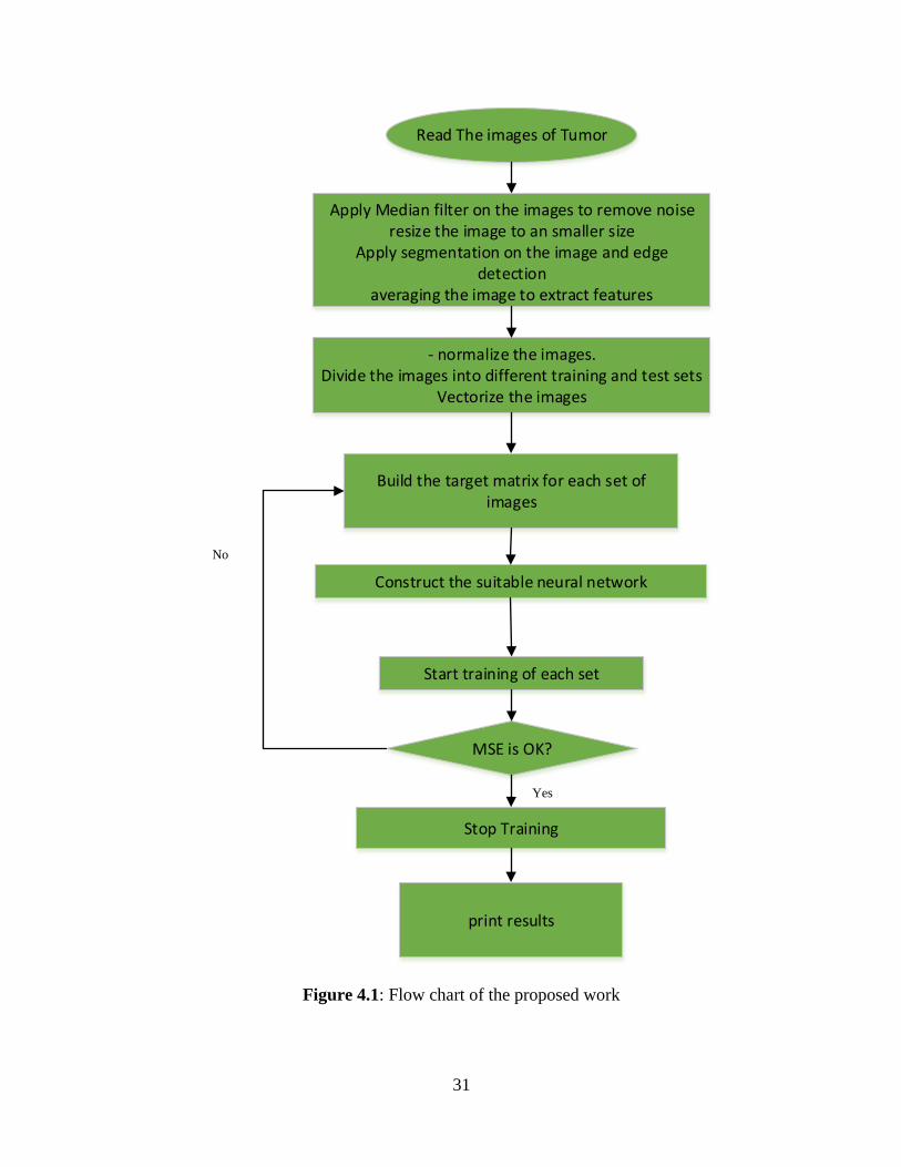
4.2 Image Processing Techniques
In order to be able to implement the methods described in the previous chapters of this work,
the flow chart of Figure 4.1 was prepared and applied for the images of the system. The
images were collected from the breast cancer database (Spanhol et al., 2016). The data base
contained a huge number of images classified by experts and divided into subfolders for two
different categories. These are the benign tumor and the malignant tumor categories. Each one
of these categories was also subdivided into four different types of tumors. A total of eight
different sub classes were obtained at the end of image classification. 560 different images for
8 different diseases were used in our implementation. The images were all treated using the
same image processing techniques in order to ensure applying same effects on all the images.
Samples of the processed images are presented in the next few figures.
Implementation of image processing techniques and ANN was applied using MATLAB script
method. A script was written that can read all images in JPEG image format, convert them into
simple gray scale image, apply median filter to the images, segment the images, compress the
image size, and normalize the images. The normalized images are then
31
Read The images of Tumor
- normalize the images.Divide the images into different training and test sets
Vectorize the images
Build the target matrix for each set of images
Construct the suitable neural network
Start training of each set
MSE is OK?
Stop Training
print results
Yes
No
Apply Median filter on the images to remove noiseresize the image to an smaller size
Apply segmentation on the image and edge detection
averaging the image to extract features
Figure 4.1: Flow chart of the proposed work
32
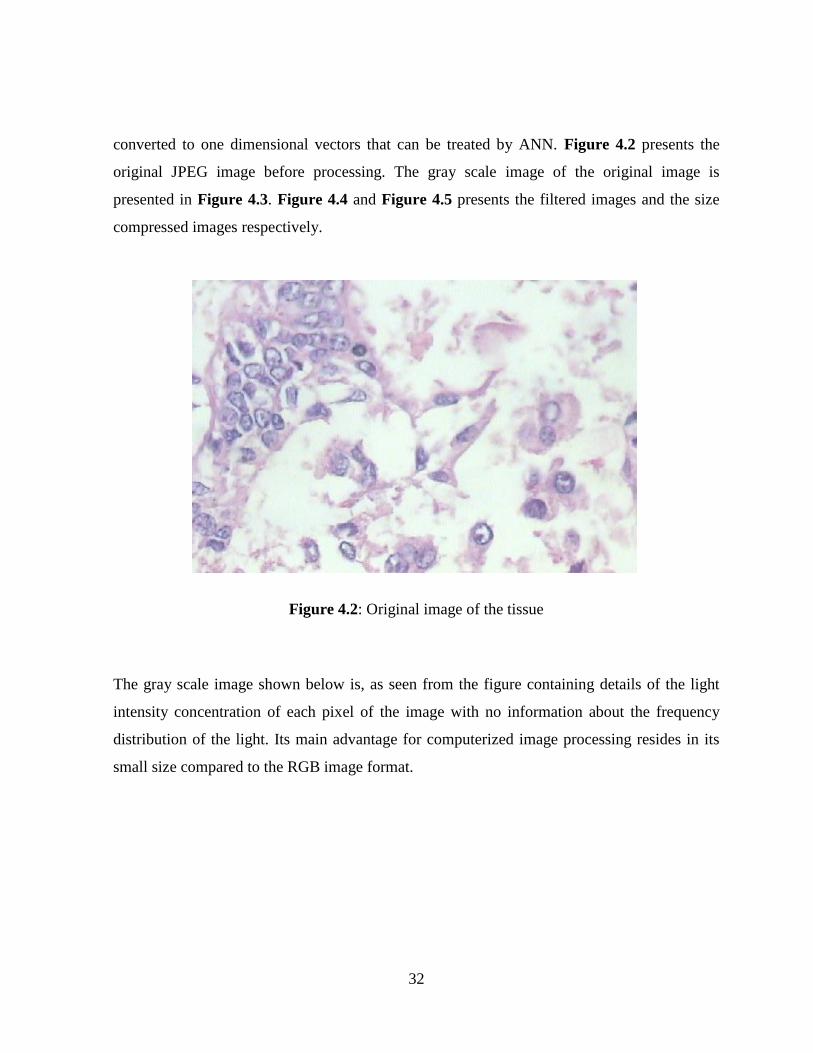
converted to one dimensional vectors that can be treated by ANN. Figure 4.2 presents the
original JPEG image before processing. The gray scale image of the original image is
presented in Figure 4.3. Figure 4.4 and Figure 4.5 presents the filtered images and the size
compressed images respectively.
Figure 4.2: Original image of the tissue
The gray scale image shown below is, as seen from the figure containing details of the light
intensity concentration of each pixel of the image with no information about the frequency
distribution of the light. Its main advantage for computerized image processing resides in its
small size compared to the RGB image format.
Original Image

33
Figure 4.3: Converted gray scale image
Figure 4.4: Filtered image using median filter
Gray Image
Filtered Image (median)

34
Figure 4.5: Small images fitted to ANN structure
4.3 Back Propagation Artificial Neural Network
In this part of the chapter, the application of the back propagation learning algorithm on the
artificial neural network for classification of medical images will be presented. The processed
images of the previous section of this chapter were presented to the neural network during the
training process. The total number of 560 different images were treated and used for the
training and test of the network. 160 images out of the 560 images were presented to the
network during the training process. The rest of images were preserved for the purpose of
testing the network. The training of the network was applied using the parameters given in the
Error! Reference source not found.. The training was initialized with arbitrary weights
given to the hidden and output layers. It took the network approximately 2 minutes and 9
seconds to converge toward the correct values of the desired output as illustrated in Figure
4.7. Figure 4.7 presents also the curve of the MSE evolution as function of the training time.
It is clear that the MSE was decreasing all the time with the training evolution.
Resized images 50*50

35
Table 4.1: Back propagation training parameters
Parameter Value Parameter Value
Network type Back propagation Learning rate 0.0002
Network size 3 layers Momentum value 0.01
Input layer 2500 MSE 9.58 ∗ 10−5
Hidden layer/s 600 Time (s) 129
Output layer 8 Epochs 325
Transfer function/s Tangent sigmoid Training efficiency 97.5%
Test efficiency 85.5 Total efficiency 89%
Figure 4.6: Training tool of the artificial neural network

36
Figure 4.7: Training MSE evolution with time
Figure 4.6 presents the ANN training tool of MATLAN where the structure of network, layers,
MSE, iterations and much other information are available. The training of the system has
shown a high training efficiency of 100% with 160 recognized images out of 160 total training
images. Table 4.2 presents the obtained output of the first sample of training images as
generated by the neural trained networks. It is obvious that all 8 diseases were recognized
correctly with high accuracy. The outputs generated from the network are similar to the
desired targets specified by the user in the beginning of the training process.
Table 4.2: Training output of first sample of images
D1 D2 D3 D4 D5 D6 D7 D8
0,932 0,018 0,007 0,010 0,007 0,004 0,005 0,004
0,021 0,575 0,016 0,001 0,008 0,010 0,001 0,002
0,087 0,116 0,978 0,015 0,009 0,004 0,014 0,004
0,001 0,002 0,008 0,979 0,005 0,003 0,003 0,011
0,003 0,028 0,003 0,009 0,981 0,033 0,022 0,004
0,091 0,001 0,002 0,004 0,010 0,936 0,001 0,010
0,001 0,018 0,000 0,002 0,003 0,001 0,774 0,010
0,000 0,006 0,002 0,003 0,007 0,012 0,022 0,984
Table 4.3 presents the output of the first test set of images after the generalization of the
network. The eight different diseases were recognized correctly with good approximation. It is
20 40 60 80 100 12010
-4
10-3
10-2
10-1
100
Time (s)
MS
E [
]

37
to mention here that a threshold of 0.5 was accepted in our work for both training and test
outputs.
Table 4.3: Test output of first sample of images
D1 D2 D3 D4 D5 D6 D7 D8
0,932 0,018 0,007 0,010 0,007 0,004 0,005 0,004
0,021 0,575 0,016 0,001 0,008 0,010 0,001 0,002
0,087 0,316 0,978 0,015 0,009 0,004 0,014 0,004
0,001 0,002 0,008 0,979 0,005 0,003 0,003 0,011
0,003 0,028 0,003 0,009 0,981 0,033 0,022 0,004
0,091 0,001 0,002 0,004 0,010 0,936 0,001 0,010
0,001 0,018 0,000 0,002 0,003 0,001 0,774 0,010
0,000 0,006 0,002 0,003 0,007 0,012 0,022 0,984
To evaluate the performance of the back propagation network under different parameters,
another experiment based on the parameters given in the Table 4.4 was carried out. The same
number of training and test images was used in this experiment. 160 training images against
400 test images were implemented. A training efficiency of 96.3% was obtained after 1 minute
of training of the network. The test efficiency of 80% was obtained. 6 incorrect predictions
were found in the training set of this structure. Samples of the training and test outputs of this
training set are presented in Table 4.5 and Table 4.6.where the red column signify an
incorrect answer.
Table 4.4: Parameters of the second ANN experiment
Parameter Value Parameter Value
Network type Back propagation Learning rate 0.2
Network size 4 layers (2 hidden) Momentum value 0.1
Input layer 2500 MSE 9.87 ∗ 10−5
Hidden layer/s 800, 250 Time (s) 62
Output layer 8 Epochs 130
Transfer function/s Tangent sigmoid Training efficiency 96.3%
Test efficiency 80% system efficiency 85%

38
Figure 4.8: Curve of MSE during the training
Table 4.5: Training output of sample images
D1 D2 D3 D4 D5 D6 D7 D8
0,986 0,010 0,007 0,012 0,001 0,001 0,000 0,001
0,015 0,981 0,016 0,007 0,002 0,028 0,004 0,001
0,013 0,014 0,983 0,014 0,004 0,002 0,003 0,002
0,002 0,003 0,013 0,979 0,010 0,001 0,001 0,016
0,005 0,004 0,001 0,013 0,982 0,007 0,011 0,013
0,007 0,007 0,002 0,002 0,002 0,891 0,009 0,005
0,001 0,006 0,000 0,001 0,009 0,005 0,982 0,051
0,002 0,001 0,004 0,002 0,002 0,009 0,013 0,607
Table 4.6: Test output of sample of images
D1 D2 D3 D4 D5 D6 D7 D8
0,986 0,010 0,007 0,012 0,001 0,001 0,000 0,001
0,015 0,981 0,016 0,007 0,002 0,028 0,004 0,001
0,013 0,014 0,983 0,014 0,004 0,002 0,003 0,002
0,002 0,003 0,013 0,979 0,010 0,001 0,001 0,016
0,005 0,004 0,001 0,013 0,982 0,007 0,011 0,013
0,007 0,007 0,002 0,002 0,002 0,891 0,009 0,005
0,001 0,006 0,000 0,001 0,009 0,005 0,982 0,513
0,002 0,001 0,004 0,002 0,002 0,009 0,013 0,131
10 20 30 40 50 6010
-4
10-3
10-2
10-1
100
Time (s)
MS
E [
]

39
Figure 4.8 above presents the MSE evolution curve during the training time that shows a
decreasing line until it reaches the pre-set value of 0.00001.
4.4 Two Step Learning Artificial Neural Network
The Two Step learning artificial neural network training algorithm was applied on the dataset.
Two step learning is used to increase the efficiency of the neural network in classification and
recognition. Instead of using the network in one stage of training, two successive training
stages are implemented in this learning process. The first stage is used to extract features of
images and store them in the weights of the hidden layer. It is normally short and takes less
than 100 epochs. The inputs and outputs of this stage are same. The obtained weights of this
stage are then used in the training of the second stage. This reduces the training time,
processing cost, and increases the efficiency of the learned network. Table 4.7 resumes the
parameters of the used Two Step learning process in this experiment. It is noticed that the two
stages were constructed of 100 hidden neurons instead of 600 in the normal Back propagation
ANN. The training time was also less than that of BPANN. The efficiency of this method was
98.4% in total. Total of 294 epochs were required to obtain a minimal MSE of 2*10-7.
Table 4.7: Parameters of the two step learning ANN
Parameter Value Parameter Value
Network type Two step learning Learning rate 0.3
Learning stages 2 Hidden 1 100
Network size 3 layers Momentum value 0.6
Input layer 2500 MSE 2.2 ∗ 10−7
Hidden layer/s 100 Time (s) 31, 23
Output layer 8 Epochs 100,194
Transfer function/s logarithmic sigmoid Training efficiency 100%
Test efficiency 97.8% system efficiency 98.4%

40
Figure 4.9 and Figure 4.10 present the MSE curves during the training of the two stage of the
neural network. It is seen that the MSE curve was decreasing during both stages.
Figure 4.9: MSE curve of the pre-training network
Figure 4.10: MSE curve of the fine tuning stage of Two step ANN
4.5 Back Propagation ANN without Median Filter
In this part of the work, the back propagation algorithm was applied on the training images
without Applying Median filter on the images. Different ANN parameters and layer neurons
were applied in this experiment. The results of the experiment were all collected and resumed
in the table 4.8 below.
5 10 15 20 25 3010
-2
10-1
100
Time (s)
MS
E (
pre
tra
inin
g)
5 10 15 2010
-10
10-5
100
Time (s)
MS
E f
inal

41
Table 4.8: Comparison of back propagation algorithm results
No Hidden neurons Moment. factor Learning rate Training result Test result
1 600 0.05 0.002 95% 81%
2 600 0.2 0.01 96% 83%
3 600 0.2 0.1 92% 78%
4 600 0.05 0.01 97% 80%
5 800 0.05 0.01 94% 82%
6 1000 0.05 0.01 90% 75%
7 500 0.05 0.01 91% 78%
8 300 0.05 0.01 92% 81%
From the table above, it is noticed that changing the parameters of the neural network can
affect the obtained results of the training. The removal of Median filter also can affect the
results with less effect because the images noise is very low. Median filter can be seen very
important in the case where some noise is existent in the images.

42
5 CHAPTER 5
CONCLUSIONS
In this work, the implementation of artificial neural network structures for the detection of
breast cancer was implemented. The use of back propagation neural network and two step
learning based neural network was presented and discussed. Breast cancer is one of the mortal
types of cancer if not treated in its early stages. 12.6% of the world’s women are possible
subjects to this disease according to different medical reports. Researches on the breast cancer
show that the early treatment of the disease is very important to save lives of millions of
women. However, the early detection of the disease using classic methods and periodic tests is
less effective due to the lack of specialized medical centres in many areas around the world.
The use of simple specialized technologies becomes indispensable in this case. This work
presented the use of artificial neural networks for the early detection of the breast cancer. The
proposed work implements two different types of neural networks in its function. These are
the back propagation neural network and the two step learning neural network. Images of
infected and healthy tissue of the women breasts were used in the presented work. Those
images were all collected from trusted medical sources and institutes. All the database images
were classified by qualified medical experts into two groups. The first group represents
healthy tissues with no signs of any malignant infections or tumors. The other group is
infected by malignant type of cancer. The two groups were also subdivided into 8 different
types of tumors. Total of 560 images were used in this work and divided into eight types of
tumors. Four types of tumors were classified as malignant tumors while the other four types
were classified as benign tumors. All database images were treated equally using same image
processing techniques to assist the function of the neural networks. Median filter and image
segmentation methods were applied to filter the images and to extract the important features
from them.
Back propagation algorithm was implemented using 1 and 2 hidden layers in the network. The
use of one hidden layer has given high speed training of the network in 129 seconds with an
overall system efficiency of 89%. The test efficiency of the system was approximately 85.5%.
The use of two hidden layers with back propagation algorithm has given faster convergence

43
for the system in 62 seconds however the efficiency was reduced to 85% instead of 89%. The
implementation of two step learning neural network has improved the results to 98% as an
average during a training time of 31 seconds.
The obtained results in this work show that the two step learning neural network is more
efficient in the detection of the cancer and its classification. It is more efficient in term of
classification accuracy and time response of the system.

44
REFERENCES
A., S. F., S., O. L., Caroline, P., & Heutte, L. (2016). A Dataset for Breast Cancer
Histopathological Image Classification. IEEE Transactions on Biomedical Engineering,
63(7), 1455–1462. https://doi.org/10.1109/TBME.2015.2496264
Ahmad, F., Isa, N. A. M., & Hussain, M. H. M. N. Z. (2013). Intelligent Breast Cancer
Diagnosis Using Hybrid GA-ANN. In 2013 Fifth International Conference on
Computational Intelligence, Communication Systems and Networks.
Anderson, D., & McNeill, G. (2010). Artificial Neural Networks Technology A DACS State-of-
the-Art Report. NewYork.
Cios, K. J., & Shields, M. E. (1997). The handbook of brain theory and neural networks.
Neurocomputing, 16(3). https://doi.org/10.1016/S0925-2312(97)00036-2
Colin, F. (1996). Artificial Neural Networks (1.1). University of Paisly.
Frank, F., Floyd, W., Wilfredo, A., & Kincaid, J. (2014). No Title. Retrieved February 10,
2017, from https://www.clear.rice.edu/elec431/projects95/lords/index.html
Hassan, J., Mariam, I., Adnan, H., Gilles, J., & Leduc, Y. (2016). Neural Network architecture
for breast cancer detection and classification. In International Multidisciplinary
Conference on Engineering Technology (pp. 37–41).
https://doi.org/10.1109/IMCET.2016.7777423
Jayaraj, S. T., Sanjana, V. G., & Darshini, V. P. (n.d.). A review on neural network and its
implementation on breast cancer detection. In 2016 International Conference on
Communication and Signal Processing.
Khashman, A., & Dimililer, K. (2007). Neural Networks Arbitration for Optimum DCT Image
Compression. In International Conference on Computer as a Tool (pp. 151–156).
Minsky, M. L., & Papert, S. A. (1969). Perceptrons. Cambridge.
Pastrana-Palma, E. D. A.-R. A. de J. (2016). Classifying microcalcifications on digital
mammography using morphological descriptors and artificial neural network. In IEEE
Conference on Computer Sciences (pp. 1–4).
45
https://doi.org/10.1109/CACIDI.2016.7785990
Singh, L., Surinder, S., & Dharmendra, S. (2016). An ANN approach for false alarm detection
in microwave breast cancer detection. In 2016 IEEE Congress on Evolutionary
Computation.
Spanhol, F., Oliveira, L. S., Petitjean, C., & Heutte, L. (2016). A Dataset for Breast Cancer
Histopathological Image Classification. In IEEE Transactions on Biomedical
Engineering (pp. 1455–1462). Retrieved from http://web.inf.ufpr.br/vri/breast-cancer-
database
Tripathy, R. K. (2013). An Investigation of The Breast Cancer Classification Using Various
Machine Learning Techniques. National Institute of Technology.