Embed Size (px)
Citation preview
Branch Flow Model
relaxations, convexification
Masoud Farivar Steven Low
Computing + Math Sciences
Electrical Engineering
Caltech
May 2012

Motivations

Global trends
1 Proliferation renewables ! Driven by sustainability ! Enabled by policy and investment

Sustainability challenge
US CO2 emission Elect generation: 40% Transportation: 20%
Electricity generation 1971-2007
1973: 6,100 TWh
2007: 19,800 TWh
Sources: International Energy Agency, 2009 DoE, Smart Grid Intro, 2008
In 2009, 1.5B people have no electricity
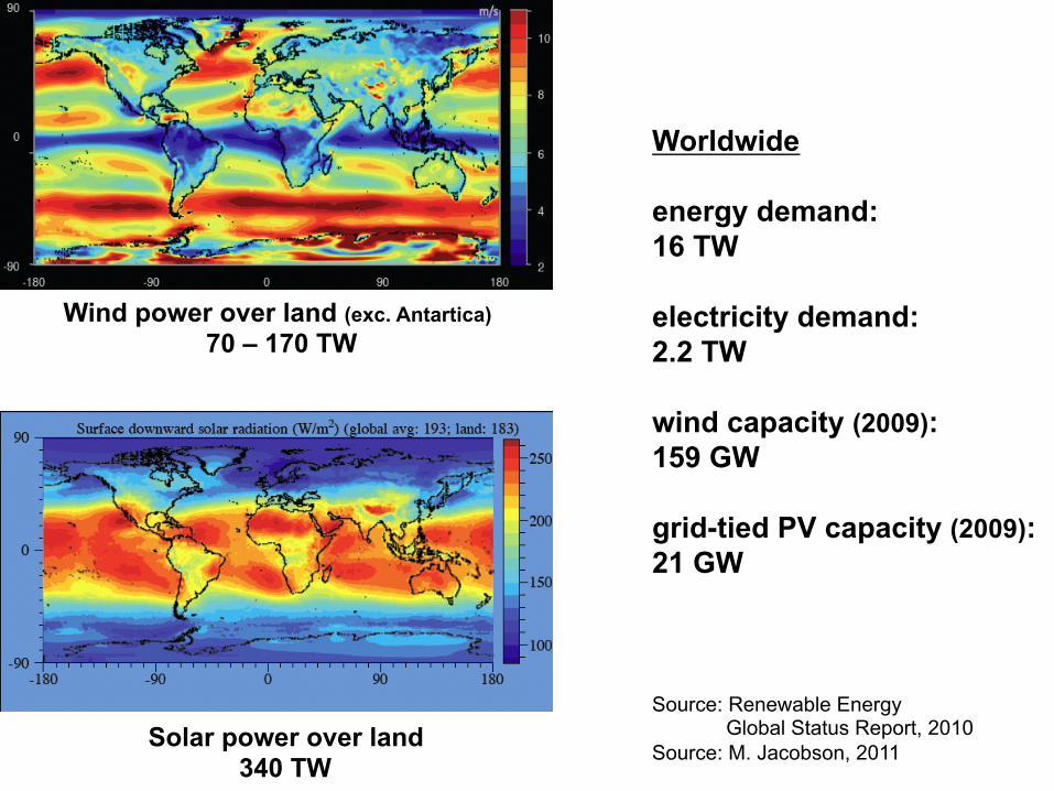
Source: Renewable Energy Global Status Report, 2010 Source: M. Jacobson, 2011
Wind power over land (exc. Antartica) 70 – 170 TW
Solar power over land 340 TW
Worldwide energy demand: 16 TW electricity demand: 2.2 TW wind capacity (2009): 159 GW grid-tied PV capacity (2009): 21 GW
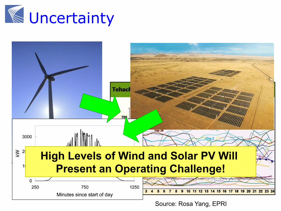
High Levels of Wind and Solar PV Will Present an Operating Challenge!
Source: Rosa Yang, EPRI
Uncertainty

Global trends
1 Proliferation of renewables ! Driven by sustainability ! Enabled by policy and investment
2 Migration to distributed arch ! 2-3x generation efficiency ! Relief demand on grid capacity

Large active network of DER
DER: PVs, wind turbines, batteries, EVs, DR loads

DER: PVs, wind turbines, EVs, batteries, DR loads
Millions of active endpoints introducing rapid large !
random fluctuations !in supply and demand!
Large active network of DER
Implications
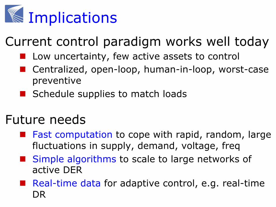
Current control paradigm works well today ! Low uncertainty, few active assets to control ! Centralized, open-loop, human-in-loop, worst-case
preventive ! Schedule supplies to match loads
Future needs ! Fast computation to cope with rapid, random, large
fluctuations in supply, demand, voltage, freq ! Simple algorithms to scale to large networks of
active DER ! Real-time data for adaptive control, e.g. real-time
DR
Key challenges
Nonconvexity ! Convex relaxations
Large scale ! Distributed algorithms
Uncertainty ! Risk-limiting approach

Optimal power flow (OPF)
OPF is solved routinely to determine ! How much power to generate where ! Market operation & pricing ! Parameter setting, e.g. taps, VARs
Non-convex and hard to solve ! Huge literature since 1962 ! Common practice: DC power flow (LP)
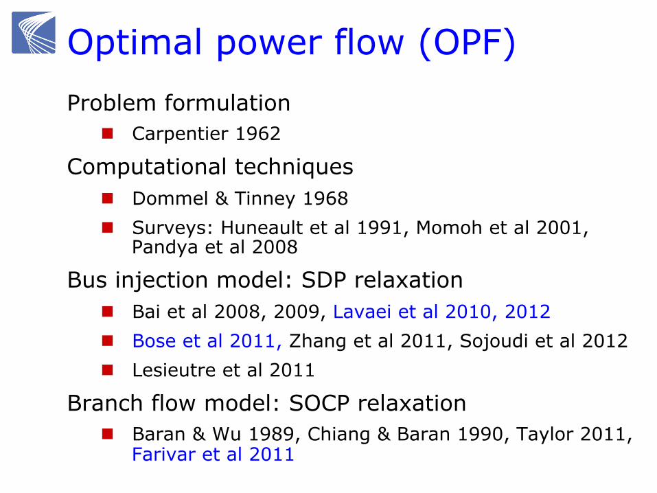
Optimal power flow (OPF) Problem formulation
! Carpentier 1962
Computational techniques ! Dommel & Tinney 1968 ! Surveys: Huneault et al 1991, Momoh et al 2001,
Pandya et al 2008
Bus injection model: SDP relaxation ! Bai et al 2008, 2009, Lavaei et al 2010, 2012 ! Bose et al 2011, Zhang et al 2011, Sojoudi et al 2012 ! Lesieutre et al 2011
Branch flow model: SOCP relaxation ! Baran & Wu 1989, Chiang & Baran 1990, Taylor 2011,
Farivar et al 2011

Application: Volt/VAR control
Motivation ! Static capacitor control cannot cope with rapid
random fluctuations of PVs on distr circuits
Inverter control ! Much faster & more frequent ! IEEE 1547 does not optimize
VAR currently (unity PF)
!"#$%#&$%'"(#)%*#)+#,"&%
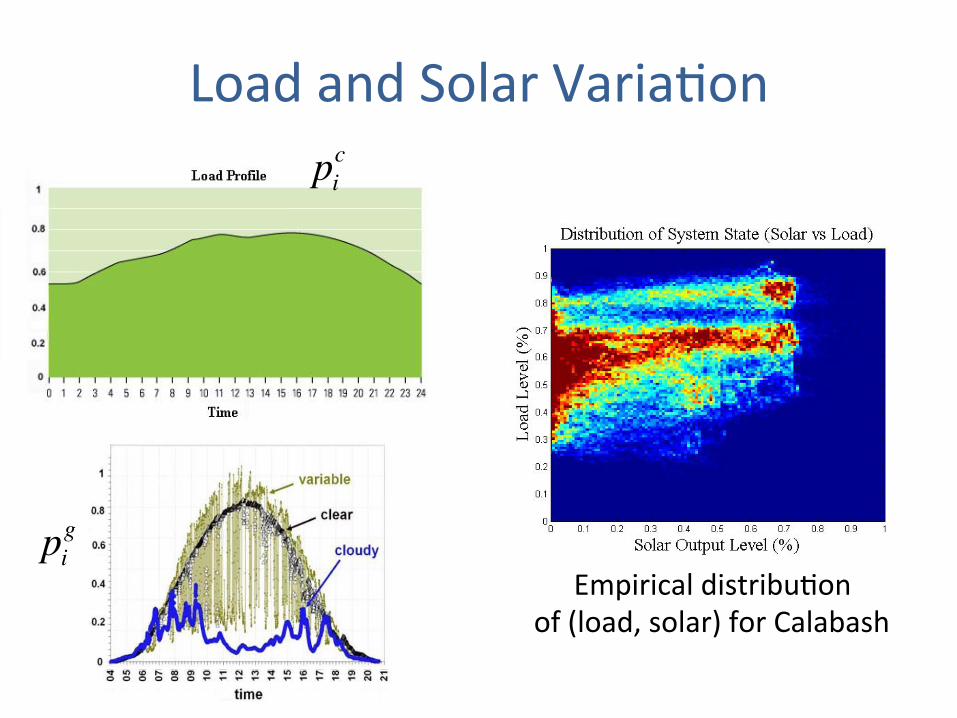
-./+)+0#(%$+12)+34,"&%%"5%6("#$7%1"(#)8%5")%9#(#3#1:%
pic
pig
'4..#);%
• <")=%)=(+#3(=%"/=)#,"&%• -&=)>;%1#?+&>1%
Outline
Branch flow model and OPF
Solution strategy: two relaxations ! Angle relaxation ! SOCP relaxation
Convexification for mesh networks
Extension

Two models
i j k
sjg sj
c
SijSjk3)#&0:%
@"A%
!Sj = Sjkk!341%%
+&B=0,"&%

Two models
i j k zij
Vi VjIijbranch current !I j = I jk
k!
bus current
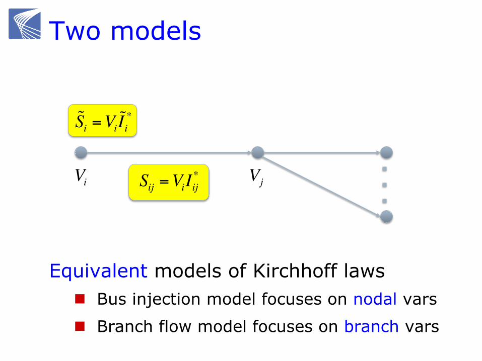
Two models
Vi Vj
!Si =Vi !Ii*
Sij =ViIij*
Equivalent models of Kirchhoff laws ! Bus injection model focuses on nodal vars
! Branch flow model focuses on branch vars

Two models
Vi Vj
!Si =Vi !Ii*
Sij =ViIij*
1. What is the model? 2. What is OPF in the model? 3. What is the solution strategy?

let’s start with something familiar
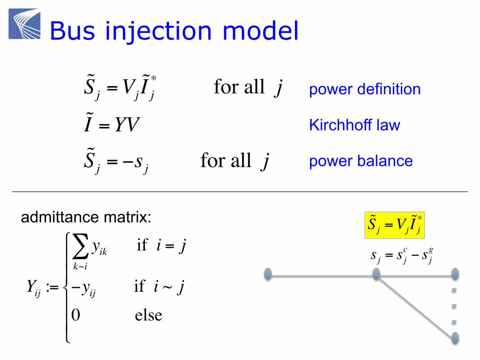
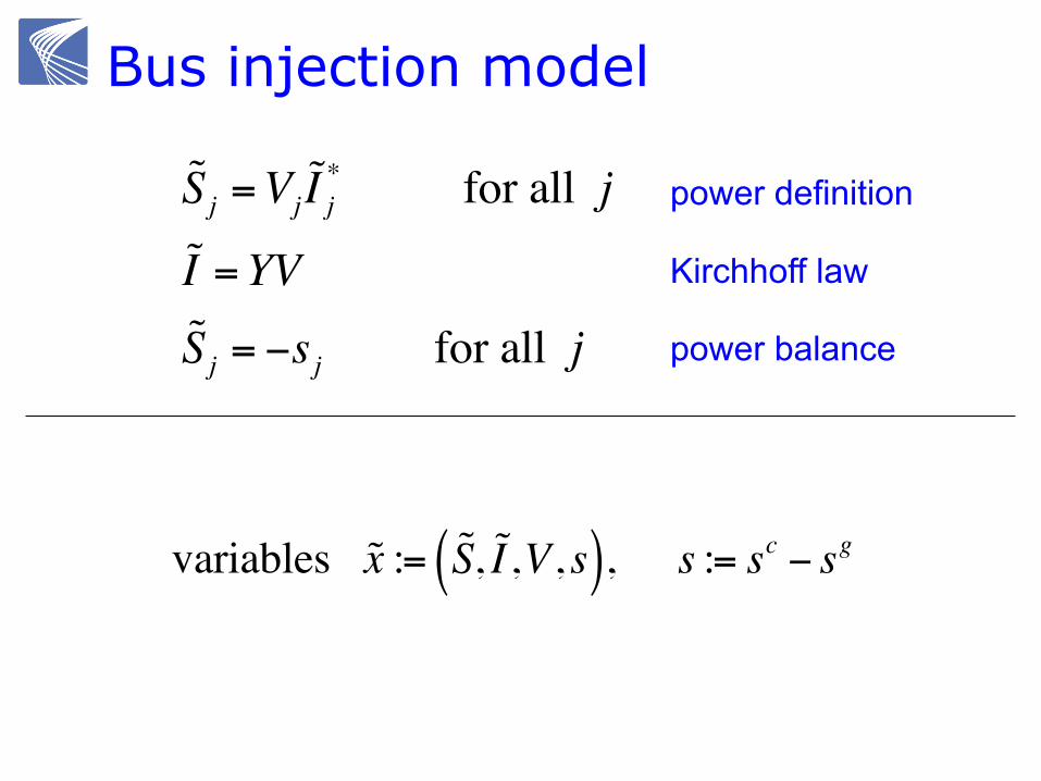
Bus injection model
!Sj =Vj!I j
* for all j!I =YV!Sj = !sj for all j
admittance matrix:
Yij :=
yikk~i! if i = j
"yij if i ~ j0 else
#
$
%%
&
%%
!Sj =Vj!I j*
sj = sjc ! sj
g
Kirchhoff law
power balance
power definition
Bus injection model
!Sj =Vj!I j
* for all j!I =YV!Sj = !sj for all j
Kirchhoff law
power balance
power definition
variables !x := !S, !I,V, s( ), s := sc ! sg
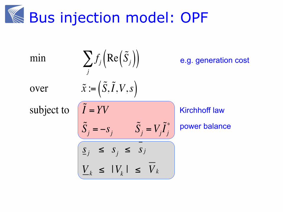
Bus injection model: OPF
min f j Re !Sj( )( )j!
over !x := !S, !I,V, s( )subject to !I =YV !Sj = "sj !Sj =Vj
!I j*
s j # sj # s j
V k # |Vk | # V k
e.g. generation cost
Kirchhoff law
power balance
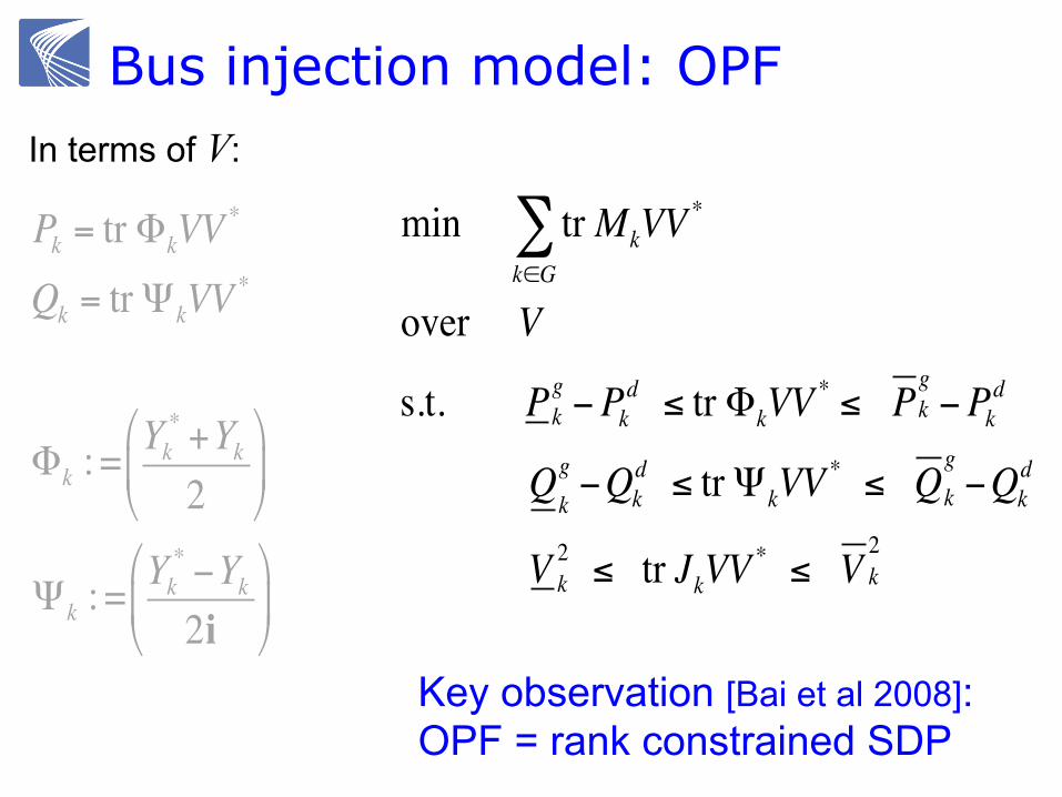
Bus injection model: OPF
Pk = tr !kVV*
Qk = tr " kVV*
!k : = Yk* +Yk2
#
$%
&
'(
" k : = Yk* )Yk2i
#
$%
&
'(
In terms of V:
min tr MkVV*
k!G"
over V
s.t. Pkg #Pk
d $ tr %kVV* $ Pk
g#Pk
d
Qkg #Qk
d $ tr & kVV* $ Qk
g#Qk
d
V k2 $ tr JkVV
* $ V k2
Key observation [Bai et al 2008]: OPF = rank constrained SDP
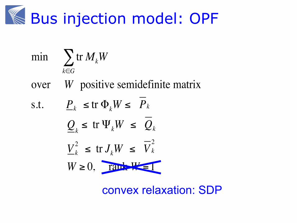
min tr MkWk!G"
over W positive semidefinite matrix
s.t. Pk # tr $kW # Pk
Qk# tr % kW # Qk
V k2 # tr JkW # V k
2
W & 0, rank W =1
Bus injection model: OPF
convex relaxation: SDP

Bus injection model: SDR Non-convex QCQP
Rank-constrained SDP
Relax the rank constraint and solve the SDP
Does the optimal solution satisfy the rank-constraint?
We are done! Solution may not be meaningful
yes no
Lavaei 2010, 2012 Radial: Bose 2011, Zhang 2011 Sojoudi 2011
Lesiertre 2011
Bai 2008

Bus injection model: summary
OPF = rank constrained SDP
Sufficient conditions for SDR to be exact
! Mesh: must solve SDR to check ! Tree: depends only on constraint pattern

Two models
Vi Vj
!Si =Vi !Ii*
Sij =ViIij*
1. What is the model? 2. What is OPF in the model? 3. What is the solution strategy?

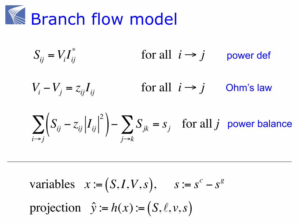
Branch flow model
Ohm’s law
Sij =ViIij* for all i! j
Vi !Vj = zij Iij for all i" j
Sij ! zij Iij2( )
i" j# ! Sjk
j"k# = sj for all j power balance
sj
sending end pwr
loss
sending end pwr
power def
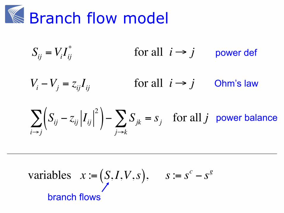
Branch flow model
Ohm’s law
Sij ! zij Iij2( )
i" j# ! Sjk
j"k# = sj for all j
Sij =ViIij* for all i! j
Vi !Vj = zij Iij for all i" j
power balance
variables x := S, I,V, s( ), s := sc ! sg
branch flows
power def
Branch flow model
Ohm’s law
Sij ! zij Iij2( )
i" j# ! Sjk
j"k# = sj for all j
Sij =ViIij* for all i! j
Vi !Vj = zij Iij for all i" j
power balance
variables x := S, I,V, s( ), s := sc ! sg
projection y := h(x) := S,!,v, s( )
power def

Sij =ViIij*
Sij = Sjkk: j~k! + zij Iij
2+ sj
c " sjgC+)0:"DE1%!#AF%
Vj =Vi ! zij IijG:.E1%!#AF%
min riji~ j! Iij
2+ !i
i! Vi
2
over (S, I,V, sg, sc )
s. t. sig " si
g " sig si " si
c vi " vi " vi
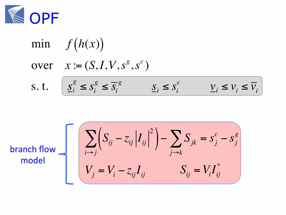
Branch flow model: OPF
)=#(%/"A=)%("11% 9*H%60"&1=)?#,"&%?"(2#>=%)=$40,"&8%%
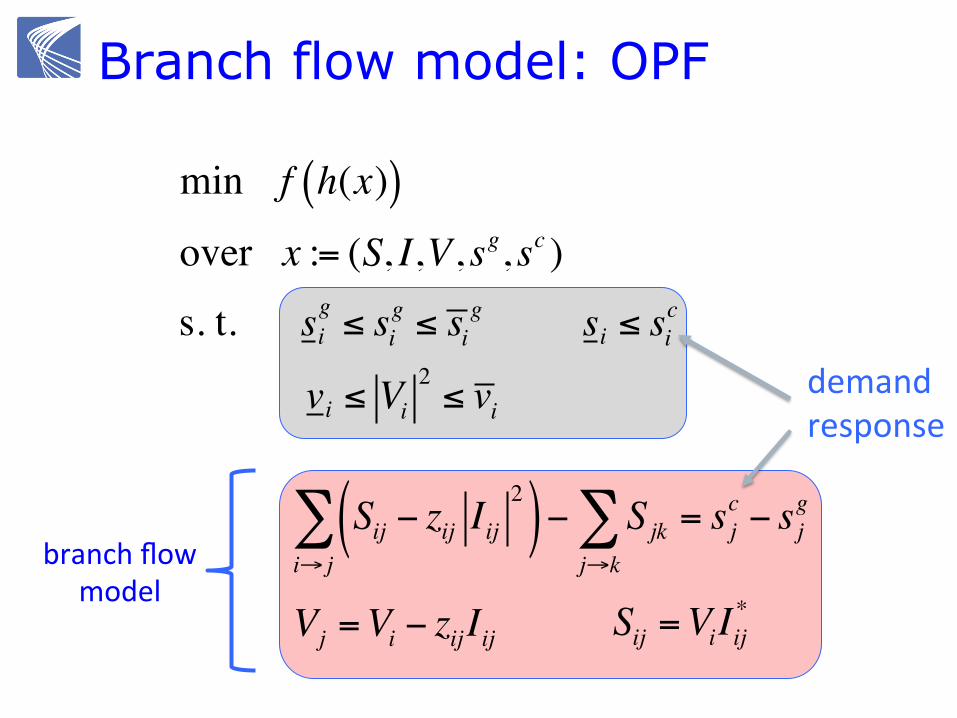
min f h(x)( )over x := (S, I,V, sg, sc )
s. t. sig ! si
g ! sig si ! si
c
vi ! Vi2! vi
Branch flow model: OPF
$=.#&$%)=1/"&1=%
Sij =ViIij*Vj =Vi ! zij Iij
3)#&0:%@"A%."$=(%
Sij ! zij Iij2( )
i" j# ! Sjk
j"k# = sj
c ! sjg

Sij =ViIij*Vj =Vi ! zij Iij
3)#&0:%@"A%."$=(%
Branch flow model: OPF
Sij ! zij Iij2( )
i" j# ! Sjk
j"k# = sj
c ! sjg
>=&=)#,"&7%*IH%0"&2)"(%
min f h(x)( )over x := (S, I,V, sg, sc )
s. t. sig ! si
g ! sig si ! si
c
vi ! Vi2! vi
Outline
Branch flow model and OPF
Solution strategy: two relaxations ! Angle relaxation ! SOCP relaxation
Convexification for mesh networks
Extension

Solution strategy
OPF nonconvex
OPF-ar nonconvex
OPF-cr convex
exact relaxation
inverse projection
for tree angle
relaxation
conic relaxation

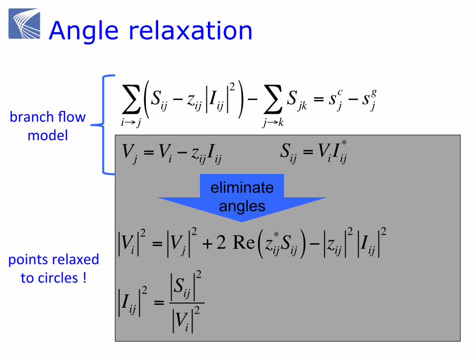
Angle relaxation
Sij =ViIij*Vj =Vi ! zij Iij
3)#&0:%@"A%."$=(%
Sij ! zij Iij2( )
i" j# ! Sjk
j"k# = sj
c ! sjg
Angle relaxation
Sij =ViIij*Vj =Vi ! zij Iij
3)#&0:%@"A%."$=(%
Sij ! zij Iij2( )
i" j# ! Sjk
j"k# = sj
c ! sjg
Vi2= Vj
2+ 2 Re zij
*Sij( )! zij2Iij
2
Iij2=Sij
2
Vi2
eliminate angles
/"+&21%)=(#J=$%%2"%0+)0(=1%K%

Vi2= Vj
2+ 2 Re zij
*Sij( )! zij2Iij
2
Iij2=Sij
2
Vi2
Angle relaxation
Sij =ViIij*Vj =Vi ! zij Iij
Sij ! zij Iij2( )
i" j# ! Sjk
j"k# = sj
c ! sjg
S, I,V, s( )

Angle relaxation
Sij =ViIij*Vj =Vi ! zij Iij
Sij ! zij Iij2( )
i" j# ! Sjk
j"k# = sj
c ! sjg
S, I,V, s( )
S,!,v, s( )
Vi2= Vj
2+ 2 Re zij
*Sij( )! zij2Iij
2
Iij2=Sij
2
Vi2
! ij := Iij2
vi := Vi2

Relaxed BF model
Sij ! zij! ij( )i" j# ! Sjk
j"k# = sj
c ! sjg
vi = vj + 2 Re zij*Sij( )! zij
2! ij
! ij =Sij
2
viL#)#&%#&$%M4%NOPO%5")%)#$+#(%&=2A")Q1%
relaxed branch flow solutions: satisfy S,!,v, s( )
Sij =ViIij*Vj =Vi ! zij Iij
3)#&0:%@"A%."$=(%
OPF
Sij ! zij Iij2( )
i" j# ! Sjk
j"k# = sj
c ! sjg
min f h(x)( )over x := (S, I,V, sg, sc )
s. t. sig ! si
g ! sig si ! si
c vi ! vi ! vi

OPF
x ! X X
min f h(x)( )over x := (S, I,V, sg, sc )
s. t. sig ! si
g ! sig si ! si
c vi ! vi ! vi
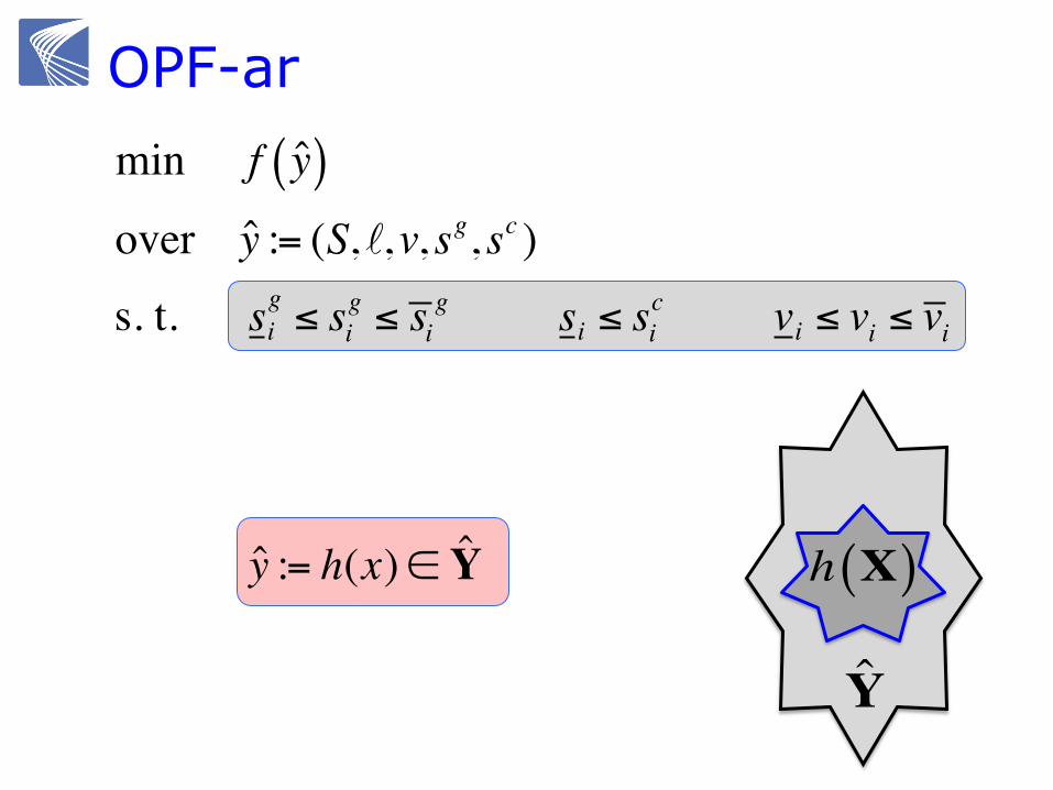
min f y( )over y := (S,!,v, sg, sc )
s. t. sig ! si
g ! sig si ! si
c vi ! vi ! vi
OPF-ar
y := h(x)! Y
Y
h X( )
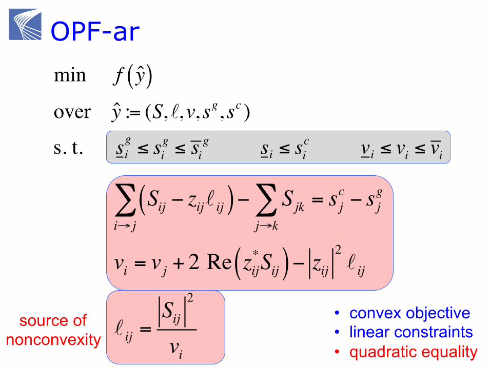
min f y( )over y := (S,!,v, sg, sc )
s. t. sig ! si
g ! sig si ! si
c vi ! vi ! vi
OPF-ar
Sij ! zij! ij( )i" j# ! Sjk
j"k# = sj
c ! sjg
vi = vj + 2 Re zij*Sij( )! zij
2! ij
! ij =Sij
2
vi
• convex objective • linear constraints • quadratic equality
source of nonconvexity

min f y( )over y := (S,!,v, sg, sc )
s. t. sig ! si
g ! sig si ! si
c vi ! vi ! vi
OPF-cr
Sij ! zij! ij( )i" j# ! Sjk
j"k# = sj
c ! sjg
vi = vj + 2 Re zij*Sij( )! zij
2! ij
! ij =Sij
2
vi" inequality ! ij !
Sij2
vi
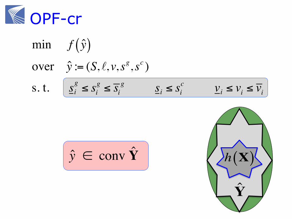
min f y( )over y := (S,!,v, sg, sc )
s. t. sig ! si
g ! sig si ! si
c vi ! vi ! vi
OPF-cr
y ! conv Y
Y
h X( )

Recap so far …
OPF nonconvex
OPF-ar nonconvex
OPF-cr convex
exact relaxation
inverse projection
for tree angle
relaxation
conic relaxation

Theorem OPF-cr is convex
! if objective is linear, then SOCP
OPF-cr is exact relaxation
f h(x)( ) := riji~ j! lij + !i
i! vi
OPF-cr is exact ! optimal of OPF-cr is also optimal for OPF-ar ! for mesh as well as radial networks ! real & reactive powers, but volt/current mags

OPF ??
Angle recovery
Y
y
OPF-ar h!!1(y)" X ?
Y
h X( )
Y
h X( )
y y
does there exist s.t. !

Theorem Inverse projection exist iff s.t.
Angle recovery
B! = " y( )
Two simple angle recovery algorithms
! centralized: explicit formula ! decentralized: recursive alg
!!!
incidence matrix; depends on topology
depends on OPF-ar solution
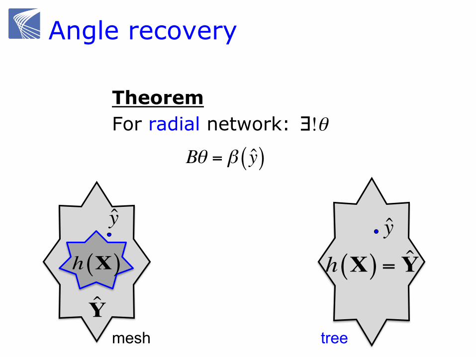
Theorem For radial network:
Angle recovery
B! = " y( )!!!
h X( ) = Yy
Y
h X( )
y
mesh tree
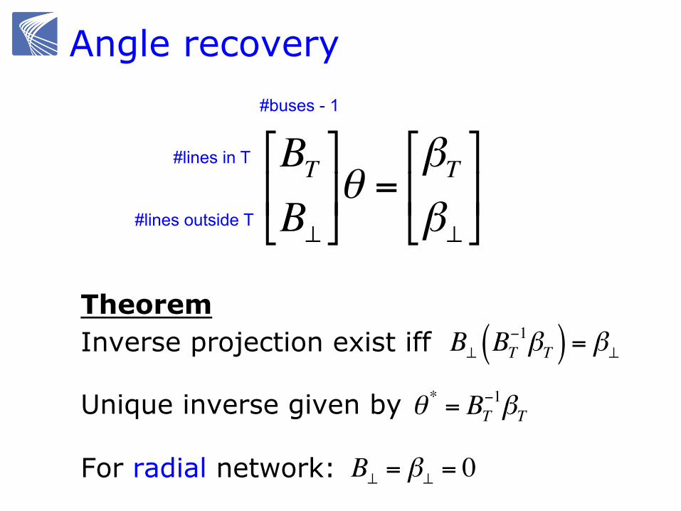
Theorem Inverse projection exist iff
Unique inverse given by
For radial network:
Angle recovery
B! BT"1!T( ) = !!
BTB!
"
#$
%
&'! =
"T"!
"
#$
%
&'
#buses - 1
#lines in T
#lines outside T
! * = BT!1"T
B! = !! = 0

OPF solution
'"(?=%GRST0)%
GRS%1"(4,"&%
H=0"?=)%#&>(=1%
radial
SOCP
• explicit formula • distributed alg
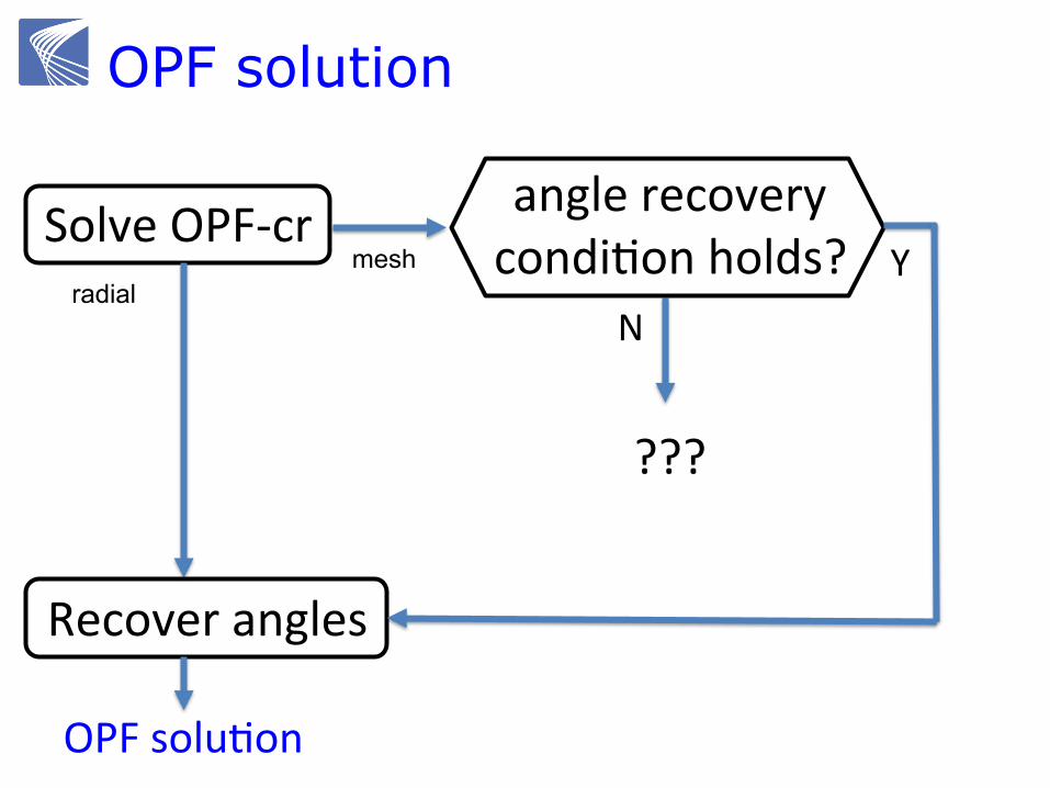
OPF solution
'"(?=%GRST0)%
UUU%
V%
GRS%1"(4,"&%
H=0"?=)%#&>(=1%
radial
#&>(=%)=0"?=);%0"&$+,"&%:"($1U% W%mesh

Outline
Branch flow model and OPF
Solution strategy: two relaxations ! Angle relaxation ! SOCP relaxation
Convexification for mesh networks
Extension

Recap: solution strategy
OPF nonconvex
OPF-ar nonconvex
OPF-cr convex
exact relaxation
inverse projection
for tree angle
relaxation
conic relaxation
??
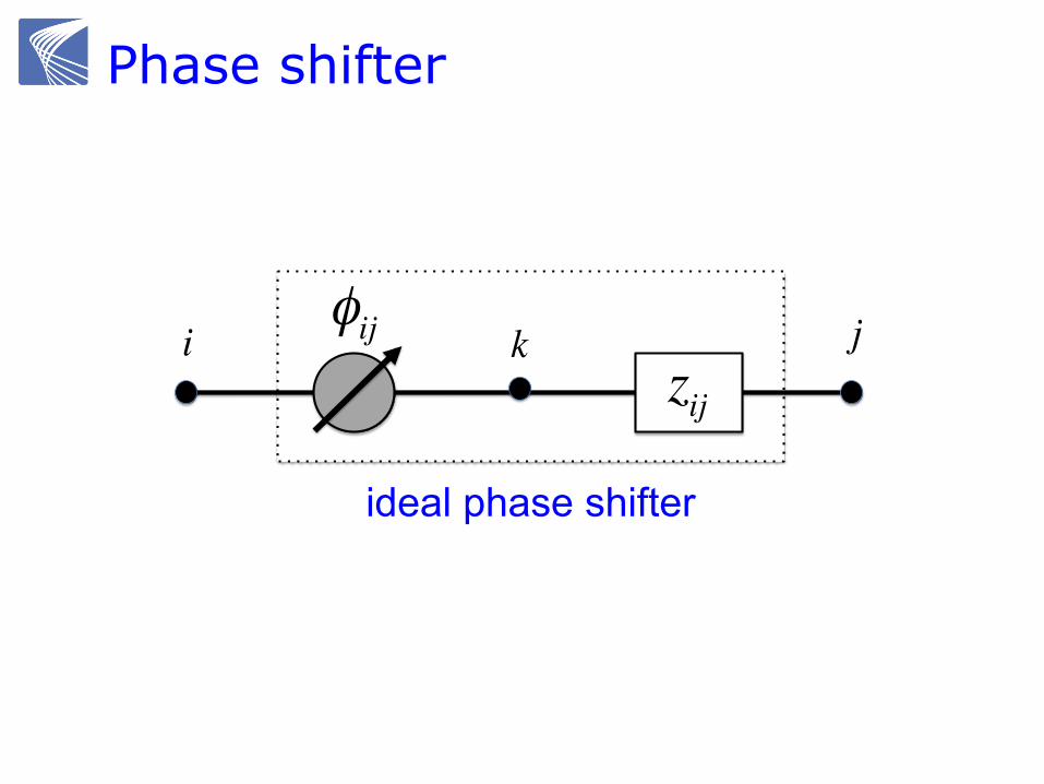
Phase shifter
ideal phase shifter
11
3) For each link (j, k) ∈ E \ ET not in the spanningtree, node j is an additional parent of k in additionto k’s parent in the spanning tree from which ∠Vk
has already been computed in Step 2.a) Compute current angle ∠Ijk using (39).b) Compute a new voltage angle θjk using the new
parent j and (40). If θjk �= ∠Vk, then anglerecovery has failed and (S, �, v, s0) is spurious.
If the angle recovery procedure succeeds in Step 3, then(S, �, v, s0) together with these angles ∠Vk,∠Ijk areindeed a branch flow solution. Otherwise, the angles ∠Vk
determined in Step 1 do not satisfy the Kirchhoff voltagelaw
�i Vi = 0 around the loop that involves the link
(j, k) identified in Step 3(b). This violates the conditionBT⊥B−1
T βT = βT⊥ in Theorem 2.
C. Radial networksRecall that all relaxed solutions in Y \ h(X) are
spurious. Our next key result shows that, for radialnetwork, h(X) = Y and hence angle relaxation is alwaysexact in the sense that there is always a unique inverseprojection that maps any relaxed solution y to a branchflow solution in X (even though X �= Y).
Theorem 4: Suppose G = T is a tree. Then1) h(X) = Y.2) given any y, θ∗ := B−1β always exists and is the
unique phase angle vector such that hθ∗(y) ∈ X.Proof: When G = T is a tree, m = n and hence
B = BT and β = βT . Moreover B is n × n and offull rank. Therefore θ∗ = B−1β always exists and, byTheorem 2, hθ∗(y) is the unique branch flow solutionin X whose projection is y. Since this holds for anyarbitrary y ∈ Y, Y = h(X).
A direct consequence of Theorem 1 and Theorem 4is that, for a radial network, OPF is equivalent to theconvex problem OPF-cr in the sense that we can obtainan optimal solution of one problem from that of the other.
Corollary 5: Suppose G is a tree. Given an optimalsolution (y∗, s∗) of OPF-cr, there exists a unique θ∗ suchthat (hθ∗(y∗), s∗) is an optimal solution of the originalOPF.
Proof: Suppose (y∗, s∗) is optimal for OPF-cr (24)–(25). Theorem 1 implies that it is also optimal for OPF-ar. In particular y∗ ∈ Y(s∗). Since G is a tree, Y(s∗) =h(X(s∗)) by Theorem 4 and hence there is a unique θ∗such that hθ∗(y∗) is a branch flow solution in X(s∗).This means (hθ∗(y∗), s∗) is feasible for OPF (10)–(11).Since OPF-ar is a relaxation of OPF, (hθ∗(y∗), s∗) is alsooptimal for OPF.
Remark 3: Theorem 1 implies that we can alwayssolve efficiently a conic relaxation OPF-cr to obtain asolution of OPF-ar, provided there are no upper boundson the power consumptions pci , q
ci . From a solution of
OPF-ar, Theorem 4 and Corollary 5 prescribe a way torecover an optimal solution of OPF for radial networks.For mesh networks, however, the solution of OPF-ar maybe spurious, i.e., there are no angles ∠Vi,∠Iij that willsatisfy the Kirchhoff laws if the angle recovery conditionin Theorem 2 fails to hold. To deal with this, we nextpropose a way to convexify the network.
VI. CONVEXIFICATION OF MESH NETWORK
In this section, we explain how to use phase shiftersto convexify a mesh network so that an extended anglerecovery condition can always be satisfied by any relaxedsolution and can be mapped to a valid branch flowsolution of the convexified network. As a consequence,the OPF for the convexified network can always besolved efficiently (in polynomial time).
A. Branch flow solutionsIn this section we study power flow solutions
and hence we fix an s. All quantities, such asx, y,X, Y, X,XT , are with respect to the given s, eventhough that is not explicit in the notation. In the nextsection, s is also an optimization variable and the setsX, Y, X,XT are for any s; c.f. the more accurate nota-tion in (4) and (5).
Phase shifters can be traditional transformers orFACTS (Flexible AC Transmission Systems) devices.They can increase transmission capacity and improvestability and power quality [37], [38]. In this paper,we consider an idealized phase shifter that only shiftsthe phase angles of the sending-end voltage and currentacross a line, and has no impedance nor limits on theshifted angles. Specifically, consider an idealized phaseshifter parametrized by φij across line (i, j), as shownin Figure 4. As before, let Vi denote the sending-end
kzij
i j!ij
Fig. 4: Model of a phase shifter in line (i, j).
voltage. Define Iij to be the sending-end current leavingnode i towards node j. Let k be the point between

Convexification of mesh networks
OPF minx
f h(x)( ) s.t. x ! X
Theorem • • Need phase shifters only outside spanning tree
X =Y
OPF-ps minx,!
f h(x)( ) s.t. x ! X
X
X
OPF-ar minx
f h(x)( ) s.t. x ! Y
Y
X
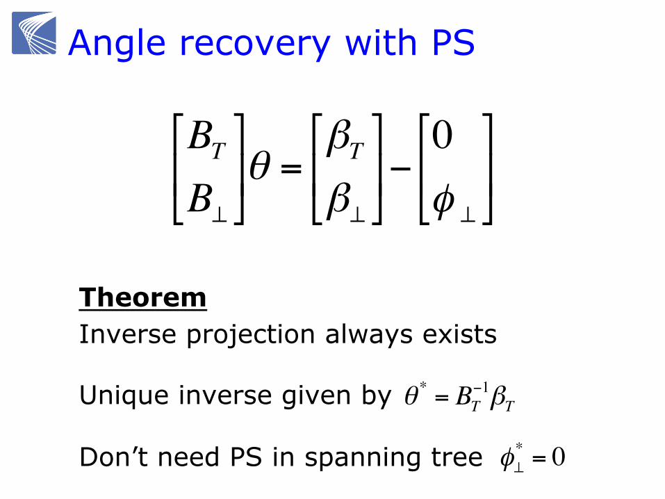
Theorem Inverse projection always exists
Unique inverse given by
Don’t need PS in spanning tree
Angle recovery with PS
BTB!
"
#$
%
&'! =
"T"!
"
#$
%
&'(
0# !
"
#$
%
&'
! * = BT!1"T
!!* = 0

OPF solution
'"(?=%GRST0)%
G/,.+X=%/:#1=%1:+Y=)1%
V%
GRS%1"(4,"&%
H=0"?=)%#&>(=1%
radial
#&>(=%)=0"?=);%0"&$+,"&%:"($1U% W%mesh
• explicit formula • distributed alg

Examples 14
No PS With phase shifters (PS)
Test cases # links Min loss Min loss # required PS # active PS Angle range (◦)
(m) (OPF, MW) (OPF-cr, MW) (m− n) |φi| > 0.1◦ [φmin,φmax]
IEEE 14-Bus 20 0.546 0.545 7 (35%) 2 (10%) [−2.1, 0.1]IEEE 30-Bus 41 1.372 1.239 12 (29%) 3 (7%) [−0.2, 4.5]IEEE 57-Bus 80 11.302 10.910 24 (30%) 19 (24%) [−3.5, 3.2]IEEE 118-Bus 186 9.232 8.728 69 (37%) 36 (19%) [−1.9, 2.0]IEEE 300-Bus 411 211.871 197.387 112 (27%) 101 (25%) [−11.9, 9.4]
New England 39-Bus 46 29.915 28.901 8 (17%) 7 (15%) [−0.2, 2.2]Polish (case2383wp) 2,896 433.019 385.894 514 (18%) 376 (13%) [−20.1, 16.8]Polish (case2737sop) 3,506 130.145 109.905 770 (22%) 433 (12%) [−21.9, 21.7]
TABLE II: Loss minimization. Min loss without phase shifters (PS) was computed using SDP relaxation of OPF
(10)–(11); min loss with phase shifters was computed using SOCP relaxations OPF-cr (24)–(23) of OPF-ar. The
“(%)” indicates the number of PS as a percentage of #links.
No PS With phase shifters (PS)
Test cases Max loadability Max loadability # required PS # active PS Angle range (◦)
(OPF) (OPF-cr) (m− n) |φi| > 0.1◦ [φmin,φmax]
IEEE 14-Bus 195.0% 195.2% 7 (35%) 6 (30%) [−0.5, 1.4]IEEE 30-Bus 156.7% 158.7% 12 (29%) 9 (22%) [−0.4, 12.4]IEEE 57-Bus 108.2% 118.3% 24 (30%) 24 (30%) [−13.1, 23.2]
IEEE 118-Bus 203.7% 204.9% 69 (37%) 64 (34%) [−16.5, 22.3]IEEE 300-Bus 106.8% 112.8% 112 (27%) 103 (25%) [−15.0, 16.5]
New England 39-Bus 109.1% 114.8% 8 (17%) 5 (11%) [−6.3, 10.6]Polish (case2383wp) 101.4% 106.6% 514 (18%) 435 (15%) [−19.6, 19.4]Polish (case2737sop) 127.6% 132.5% 770 (22%) 420 (12%) [−16.7, 17.0]
TABLE III: Loadability maximization. Max loadability without phase shifters (PS) was computed using SDP
relaxation of OPF (10)–(11); max loadability with phase shifters was computed using SOCP relaxations OPF-cr
(24)–(23) of OPF-ar. The “(%)” indicates the number of PS as a percentage of #links.
the corresponding unique (hθ(y), s) that was an optimal
solution of OPF for the convexified network.
To place the phase shifters, we have used a minimum
spanning tree of the network where the weights on the
lines are their reactance values. In Tables II and III, we
report the number m − n of phase shifters potentially
required on every link outside the minimum spanning
tree, as well as the number of active phase shifters (i.e.,
those with a phase angles greater than 0.1◦) and the range
of their phase angles at optimality. The optimal choice
of spanning tree, e.g., to minimize the number of active
phase shifters and the range of their angles, remains an
open problem.
We also report the optimal objective values of OPF
with and without phase shifters in Tables II and III.
The optimal values of OPF without phase shifters were
obtained by implementing the SDP formulation and
relaxation proposed in [16] for solving OPF (10)–(11).
We verified the exactness of the SDP relaxation by
checking if the solution matrix was of rank one [13],
[16]. In all test cases, the SDP relaxation was exact and
hence the optimal objective values reported were indeed
the optimal value of OPF (10)–(11). As expected, the
optimal loss (Table II) and the optimal loadability (Table
III) for OPF-ar (equivalently OPF-cr) are, respectively,
lower and higher than the corresponding optimal values
of OPF. This confirms that the solutions obtained from
the SOCP relaxation are infeasible for the original OPF
but can be implemented with phase shifters, at a lower
loss or higher loadability.
The SDP relaxation requires the addition of small
resistances (10−6pu) to every link that has a zero
resistance in the original model, as suggested in [13].
This addition is, on the other hand, not required for the
SOCP relaxation: OPF-cr is tight with respect to OPF-ar
with or without this addition. For comparison, we report
the results where the same resistances are added for both
the SDP and SOCP relaxations.
Summary. From Tables II and III:
1) Across all test cases, the convexified networks
have higher performance (lower minimum loss and
higher maximum loadability) than the original net-
works. More important than the modest perfor-
mance improvement, convexification is design for
simplicity: it guarantees an efficient solution for
optimal power flow.
2) The networks are (mesh but) very sparse, with the
ratios m/(n + 1) of the number of lines to the
With PS

Examples
With PS
14
No PS With phase shifters (PS)
Test cases # links Min loss Min loss # required PS # active PS Angle range (◦)
(m) (OPF, MW) (OPF-cr, MW) (m− n) |φi| > 0.1◦ [φmin,φmax]
IEEE 14-Bus 20 0.546 0.545 7 (35%) 2 (10%) [−2.1, 0.1]IEEE 30-Bus 41 1.372 1.239 12 (29%) 3 (7%) [−0.2, 4.5]IEEE 57-Bus 80 11.302 10.910 24 (30%) 19 (24%) [−3.5, 3.2]IEEE 118-Bus 186 9.232 8.728 69 (37%) 36 (19%) [−1.9, 2.0]IEEE 300-Bus 411 211.871 197.387 112 (27%) 101 (25%) [−11.9, 9.4]
New England 39-Bus 46 29.915 28.901 8 (17%) 7 (15%) [−0.2, 2.2]Polish (case2383wp) 2,896 433.019 385.894 514 (18%) 376 (13%) [−20.1, 16.8]Polish (case2737sop) 3,506 130.145 109.905 770 (22%) 433 (12%) [−21.9, 21.7]
TABLE II: Loss minimization. Min loss without phase shifters (PS) was computed using SDP relaxation of OPF
(10)–(11); min loss with phase shifters was computed using SOCP relaxations OPF-cr (24)–(23) of OPF-ar. The
“(%)” indicates the number of PS as a percentage of #links.
No PS With phase shifters (PS)
Test cases Max loadability Max loadability # required PS # active PS Angle range (◦)
(OPF) (OPF-cr) (m− n) |φi| > 0.1◦ [φmin,φmax]
IEEE 14-Bus 195.0% 195.2% 7 (35%) 6 (30%) [−0.5, 1.4]IEEE 30-Bus 156.7% 158.7% 12 (29%) 9 (22%) [−0.4, 12.4]IEEE 57-Bus 108.2% 118.3% 24 (30%) 24 (30%) [−13.1, 23.2]
IEEE 118-Bus 203.7% 204.9% 69 (37%) 64 (34%) [−16.5, 22.3]IEEE 300-Bus 106.8% 112.8% 112 (27%) 103 (25%) [−15.0, 16.5]
New England 39-Bus 109.1% 114.8% 8 (17%) 5 (11%) [−6.3, 10.6]Polish (case2383wp) 101.4% 106.6% 514 (18%) 435 (15%) [−19.6, 19.4]Polish (case2737sop) 127.6% 132.5% 770 (22%) 420 (12%) [−16.7, 17.0]
TABLE III: Loadability maximization. Max loadability without phase shifters (PS) was computed using SDP
relaxation of OPF (10)–(11); max loadability with phase shifters was computed using SOCP relaxations OPF-cr
(24)–(23) of OPF-ar. The “(%)” indicates the number of PS as a percentage of #links.
the corresponding unique (hθ(y), s) that was an optimal
solution of OPF for the convexified network.
To place the phase shifters, we have used a minimum
spanning tree of the network where the weights on the
lines are their reactance values. In Tables II and III, we
report the number m − n of phase shifters potentially
required on every link outside the minimum spanning
tree, as well as the number of active phase shifters (i.e.,
those with a phase angles greater than 0.1◦) and the range
of their phase angles at optimality. The optimal choice
of spanning tree, e.g., to minimize the number of active
phase shifters and the range of their angles, remains an
open problem.
We also report the optimal objective values of OPF
with and without phase shifters in Tables II and III.
The optimal values of OPF without phase shifters were
obtained by implementing the SDP formulation and
relaxation proposed in [16] for solving OPF (10)–(11).
We verified the exactness of the SDP relaxation by
checking if the solution matrix was of rank one [13],
[16]. In all test cases, the SDP relaxation was exact and
hence the optimal objective values reported were indeed
the optimal value of OPF (10)–(11). As expected, the
optimal loss (Table II) and the optimal loadability (Table
III) for OPF-ar (equivalently OPF-cr) are, respectively,
lower and higher than the corresponding optimal values
of OPF. This confirms that the solutions obtained from
the SOCP relaxation are infeasible for the original OPF
but can be implemented with phase shifters, at a lower
loss or higher loadability.
The SDP relaxation requires the addition of small
resistances (10−6pu) to every link that has a zero
resistance in the original model, as suggested in [13].
This addition is, on the other hand, not required for the
SOCP relaxation: OPF-cr is tight with respect to OPF-ar
with or without this addition. For comparison, we report
the results where the same resistances are added for both
the SDP and SOCP relaxations.
Summary. From Tables II and III:
1) Across all test cases, the convexified networks
have higher performance (lower minimum loss and
higher maximum loadability) than the original net-
works. More important than the modest perfor-
mance improvement, convexification is design for
simplicity: it guarantees an efficient solution for
optimal power flow.
2) The networks are (mesh but) very sparse, with the
ratios m/(n + 1) of the number of lines to the
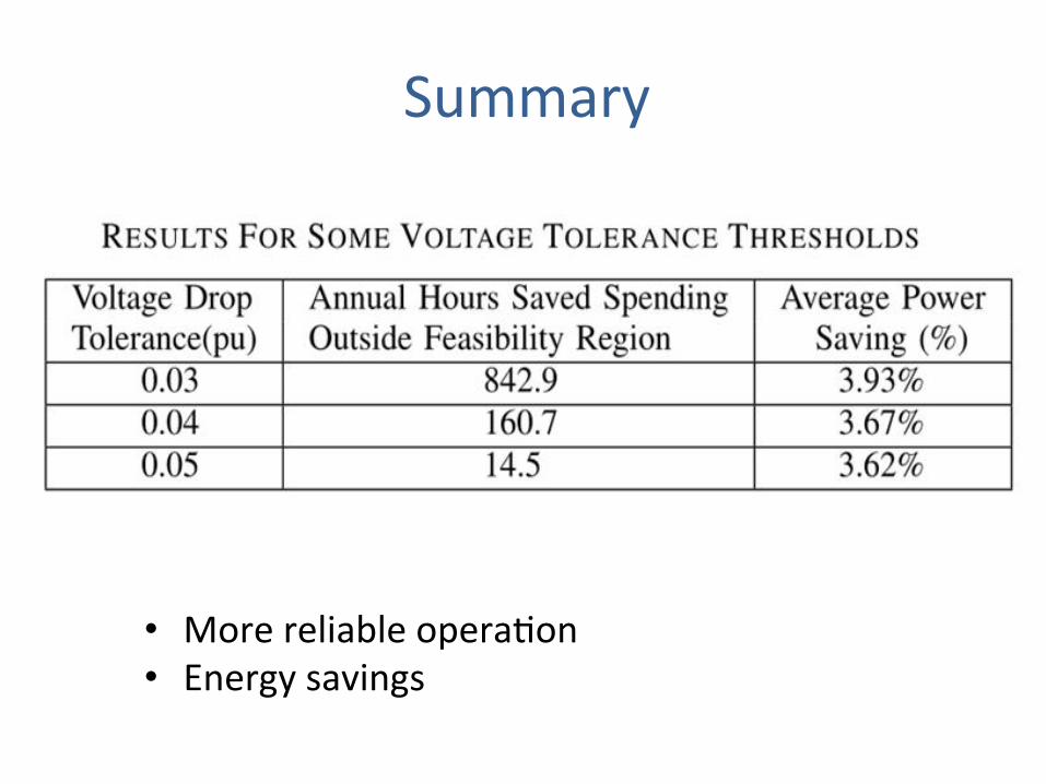
Key message
Radial networks computationally simple
! Exploit tree graph & convex relaxation ! Real-time scalable control promising
Mesh networks can be convexified
! Design for simplicity ! Need few (?) phase shifters (sparse topology)
Outline
Branch flow model and OPF
Solution strategy: two relaxations ! Angle relaxation ! SOCP relaxation
Convexification for mesh networks
Extension
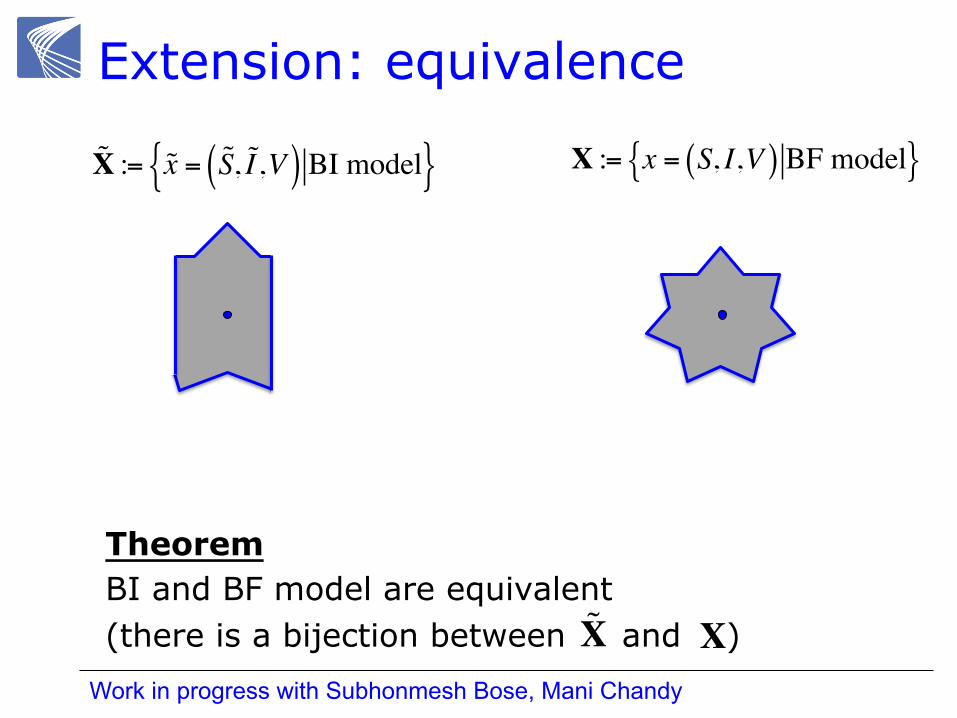
Extension: equivalence
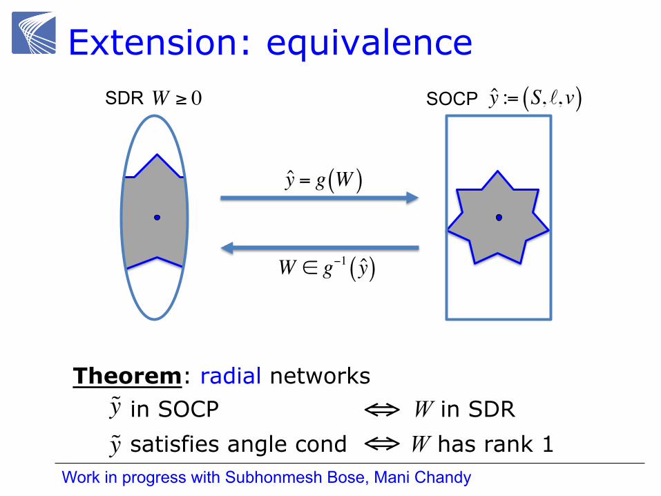
Work in progress with Subhonmesh Bose, Mani Chandy
Theorem BI and BF model are equivalent (there is a bijection between and )
!X X
!X := !x = !S, !I,V( ) BI model{ } X := x = S, I,V( ) BF model{ }
Extension: equivalence
Work in progress with Subhonmesh Bose, Mani Chandy
Theorem: radial networks in SOCP W in SDR satisfies angle cond W has rank 1
!y
SDR W ! 0 SOCP y := S,!,v( )
y = g W( )
W ! g"1 y( )
!y!!