Brain-Tumor Interaction Biophysical Models for Medical Image

University of PennsylvaniaScholarlyCommons

Departmental Papers (MEAM) Department of Mechanical Engineering &Applied Mechanics

12-1-2008

Brain-Tumor Interaction Biophysical Models forMedical Image RegistrationCosmina HogeaUniversity of Pennsylvania

Christos DavatzikosUniversity of Pennsylvania, [email protected]

George BirosUniversity of Pennsylvania, [email protected]

Copyright The American Ceramic Society. Reprinted from Siam Journal of Scientific Computing, Volume 30, Issue 6, December 2008, pages3050-3072.Publisher URL: http://dx.doi.org/10.1137/07069208X

This paper is posted at ScholarlyCommons. http://repository.upenn.edu/meam_papers/163For more information, please contact [email protected].

http://repository.upenn.edu

http://repository.upenn.edu/meam_papers

http://repository.upenn.edu/meam

http://repository.upenn.edu/meam

http://repository.upenn.edu/meam_papers/163

mailto:[email protected]

Copyright © by SIAM. Unauthorized reproduction of this article is prohibited.

SIAM J. SCI. COMPUT. c© 2008 Society for Industrial and Applied MathematicsVol. 30, No. 6, pp. 3050–3072

BRAIN–TUMOR INTERACTION BIOPHYSICAL MODELS FORMEDICAL IMAGE REGISTRATION∗

COSMINA HOGEA† , CHRISTOS DAVATZIKOS† , AND GEORGE BIROS‡

Abstract. State-of-the art algorithms for deformable image registration are based on the min-imization of an image similarity functional that is regularized by adding a penalty term on thedeformation map. The penalty function typically represents a smoothness regularization. In thisarticle, we use a constrained optimization formulation in which the image similarity functional iscoupled to a biophysical model. This formulation is pertinent when the data have been generated byimaging tissue that undergoes deformations due to an actual biophysical phenomenon. Such is thecase of coregistering tumor-bearing brain images from the same individual. We present an approxi-mate model that couples tumor growth with the mechanical deformations of the surrounding braintissue. We consider primary brain tumors—in particular, gliomas. Glioma growth is modeled by areaction-advection-diffusion PDE, with a two-way coupling with the underlying tissue elastic defor-mation. Tumor bulk, infiltration, and subsequent mass effects are not regarded separately but arecaptured by the model itself in the course of its evolution. Our formulation allows for updating thetumor diffusion coefficient following structural displacements caused by tumor growth/infiltration.Our forward problem implementation builds on the PETSc library of Argonne National Laboratory.Our reformulation results in a very small parameter space, and we use the derivative-free optimizationlibrary APPSPACK of Sandia National Laboratories. We test the forward model and the optimizationframework by using landmark-based similarity functions and by applying it to brain tumor datafrom clinical and animal studies. State-of-the-art registration algorithms fail in such problems due toexcessive deformations. We compare our results with previous work in our group, and we observedup to 50% improvement in landmark deformation prediction. We present preliminary validationresults in which we were able to reconstruct deformation fields using four degrees of freedom. Ourstudy demonstrates the validity of our formulation and points to the need for richer datasets andfast optimization algorithms.

Key words. medical image registration, tumor growth, deformable registration, soft-tissuesimulations

AMS subject classifications. 65N50, 65Y05, 68W10, 68W15

DOI. 10.1137/07069208X

1. Introduction. Medical image registration (see Figure 2) involves the con-struction of point-correspondences between a set of images: given a target image τ ,a series of images σ(t) parametrized by time t, and an image similarity functionalJ (τ, σ), we would like to construct a deformation map ψ∗(t) such that

(1.1) ψ∗ = arg minψ

J (σ ◦ ψ, τ) + R(ψ).

The penalty term R is introduced to generate anatomy-preserving deformations.Typically, R represents an energy term that ensures that ψ is a diffeomorphism[6, 11, 18, 43]. We do not attempt to review the extensive literature on formulations

∗Received by the editors May 16, 2007; accepted for publication (in revised form) June 16, 2008;published electronically October 13, 2008. A preliminary version of this article was presented at the2007 SIAM Conference on Computational Science and Engineering [31].

http://www.siam.org/journals/sisc/30-6/69208.html†Section of Biomedical Image Analysis, Department of Radiology, University of Pennsylvania,

Philadelphia, PA 19104 ([email protected], [email protected]).‡Departments of Mechanical Engineering and Applied Mechanics, Bioengineering, and Computer

and Information Science, University of Pennsylvania, Philadelphia, PA 19104 ([email protected]).

3050


BRAIN IMAGE REGISTRATION 3051

and solution methodologies for (1.1). An excellent introduction on this topic can befound in [44].

In this article, we expand our work in [29] and discuss a formulation for the casein which ψ is related to a biophysical phenomenon, the so-called mass effect: themechanical deformation of healthy brain tissue due to cancerous tumor growth. Wereformulate (1.1) by replacing R with biophysical constraints on ψ:

(1.2) (ψ∗,φ∗, g∗) = arg minψ,φ,g

J (σ ◦ ψ, τ) subject to F (φ,ψ, g) = 0.

In addition to the map ψ, we have introduced the biophysical variables φ and un-known parameters g . The nonlinear map F represents the biophysical model, areaction-advection-diffusion tumor growth model coupled to elasticity. In the brain–tumor interaction case, φ comprises two components: the tumor concentration andthe displacement. g consists of the diffusion and reaction coefficients, parametriza-tions of the initial tumor concentration, and the force coupling between the tumor andthe tissue. We use a landmark-based similarity functional J , which is mathematicallyequivalent to having discrete observations on ψ.

The main advantage of the constrained optimization formulation is that it incor-porates problem-specific prior information—instead of a generic R—related to theunderlying biophysical phenomenon. By using more informed priors, we can producecomplex deformation maps using small parameter spaces (in the case we discuss inthis paper, we use only four parameters).1

The main drawback of our approach is that strong priors may lead to strong bias—that is, if they are wrong. Indeed, there is significant uncertainty associated withthe exact form of F and its interindividual variability. Additional drawbacks of ourapproach over standard regularization techniques include computational challenges insimulating F and the fact that our formulation is not applicable to image registrationacross different individuals since there is no underlying physical deformation thatfollows a biophysical law. In the following, we describe the clinical problem, thebiophysical model, the related work, our contributions, and the limitations in ourapproach.

Motivation. More than 50% of primary brain tumors are gliomas, which are sel-dom treatable with resection, and which ultimately progress to high-grade tumors,leading to death in only 6–12 months [1]. A better understanding of the characteristicsof the progression of brain cancer, based on phenotypic cancer profiles derived fromimaging, histopathology, and other sources, can help to determine predictive factorsfor cancer invasion. A significant tool for understanding such cancer profiles is theconstruction of statistical atlases (“an average brain”).

Statistical atlases of brain function and structure have been widely used as ameans of integrating diverse information about anatomical and functional variabil-ity into a canonical coordinate space (often called a stereotactic space) for betterunderstanding and diagnosing of brain diseases [5, 13]. In the case of brain tumorpatients, such atlases have the potential to assist surgical and treatment planning. Inorder to construct and use brain tumor atlases, tumor-bearing patient images mustbe coregistered to normal brain images or a statistical atlas; i.e., a transformation

1The constrained formulation can be viewed as a nonlinear transformation on ψ. Instead ofsolving for ψ, we solve for g . If we knew the Lagrange multipliers associated with the Euler–Lagrange optimality conditions for (1), then (1.2) would be just a special case of (1.1). But theLagrange multipliers are not known. Thus, (1.2) is different from (1.1) in both analytical andcomputational aspects.


3052 COSMINA HOGEA, CHRISTOS DAVATZIKOS, AND GEORGE BIROS

(a) (b) (c)

Fig. 1. Image registration. Given two images (a) and (b) we would like to find anatomicalcorrespondences between them. Image (a) is an axial slice from an MR (magnetic resonance) imageof a patient with tumor. Image (b) can be a statistical atlas, or an MR image of the patient beforethe tumor occurrence. Mapping image (a) to image (b) is unusually hard because of the topologicaldifferences and the large deformations due to the presence of the tumor. If one uses standarddeformable registration methods, there will be significant errors, particularly in areas near the tumor.In image (c), we show a second example, an axial slice from an MR image of a patient diagnosedwith Glioblastoma multiforme grade IV. This image illustrates the highly infiltrative nature of suchtumors which leads to a poorly defined brain–tumor interface and a strong mass effect.

(a) (b) (c) (d)

Fig. 2. Biophysically constrained registration of tumor-bearing brain images.

Schematic illustration of a multistep simulation designed to improve the deformable registrationprocess from tumor-bearing patient images to normal brain templates. Instead of attempting to di-rectly register two highly dissimilar images (images (a) and (d)), we construct a tumor-bearing brainatlas (image (b)) and then register the tumor-bearing template to the actual patient image to obtainimage (c). In this way, the original problem of constructing a map between two highly dissimilarimages is the composition of two deformations: (a) to (b) and (b) to (d). In this article, we considerthe simpler problem of constructing a deformation map between images of a single individual takenat different points in time.

must be constructed between the image with the brain tumor and a given normalbrain template. Existing brain image registration methods that attempt to directlyregister two such objects typically come up short in the presence of large tumors andsubsequent mass effect, such as the case depicted in Figure 1.

Here, we present a scheme that couples a mass-effect model with image registra-tion, as depicted in Figure 2. To aid the registration process, particularly in areasclose to the tumor, it is helpful to first construct a brain atlas that has tumor andmass effects similar to the images of the patients in our study. Subsequent deformableregistration is than more likely to better match the atlas to the patient’s images, sinceit has to solve a problem involving two brains that are relatively similar, comparedto matching a normal atlas with a highly deformed brain [12, 15, 37]. This involves a



simulation pipeline in which tumor simulation is the first step, followed by registration,as illustrated schematically in Figure 2.2

1.1. Related work. Biophysically induced deformations have motivated theform of the smoothness regularization term in (1.1). Indeed, researchers often injectbiomechanical information, such as elastic constants and anisotropy directions, into R[16,33,40,48,55]. This, however, is not equivalent to having the correct biophysics, asmultiphysics couplings, boundary conditions, and distributed forces are not includedin R. To our knowledge, the only work similar to ours is [38], the authors of whichconsider a mechanical model (without tumors) for parenchymal shift. The inversionparameters are distributed forces.

Tumor growth models. Most of the work in tumor growth models has involvedin vitro experimental setups (to allow for validation). The two main approaches arediscrete [34] and continuous [3]. Cellular automata (CA), or lattice-based models,belong to the discrete setting. Probabilistic phenomenological rules are used for thespatiotemporal evolution of each cell (e.g., mitosis, apoptosis, chemotaxis, randommotion). The continuous approach is typically based on macroscopic conservation lawsexpressed via PDEs [14]. Another approach involves reaction-diffusion models [50,52].More complex models have multiple species, take into account cellular heterogeneity,and incorporate mechanical effects in tissues [4, 10,52].

Brain–tumor interaction. In [26, 28, 46], a purely mechanical model was used tosimulate the tumor–brain interface evolution and the mass effect. The brain tissuewas modeled as a nonlinearly elastic material. A cavity representing the tumor wasintroduced and a pressure-like Neumann condition was used to model tumor-inducedinterface forces. This method has two main limitations: (1) it has difficulty capturingmore irregularly shaped tumors (the simulated tumors are generally quasi-spherical);and (2) it provides no information about the actual tumor evolution and its infiltrationinto healthy tissue. In [12], the authors have used an approach similar to ours: theymodeled the mass effect caused by the tumor bulk and added a separate reaction-diffusion model (similarly to [24, 50, 52]) to account for the tumor infiltrative partonly. In their method the tumor reaction-diffusion equation is decoupled from theelasticity equations and the diffusion coefficient. No optimization framework wasused in that work.

1.2. Contributions and limitations. Given a time sequence of tumor-bearingimages from the same individual we seek to coregister them. Toward that goal, wepropose a model that couples glioma growth with the deformation of the brain tissue.Building upon the work of [50] and our own work [29], glioma growth is modeled viaa nonlinear reaction-advection-diffusion equation coupled to an elastic deformationmodel (ten variables per grid point). The overall modeling framework results in astrongly coupled nonlinear system of PDEs. The main differences compared to priorwork are that (1) there is no sharp-interface separation between a tumor bulk and aninfiltrative part; (2) the tissue deformation causes spatial changes in the distributionof the diffusion coefficient and advects the tumor concentration; and (3) the solver iscoupled with the image-registration optimization problem. Besides synthetic datasets,we use data from clinical and animal studies for the preliminary validation of ourmodel.

2Due to its complexity and high computational cost, our approach is more appropriate for at-las construction and pre- and postoperative analysis rather than for open MR-type intraoperativeregistration (see [55]).



In a nutshell, the main contributions of this paper are as follows:

• A forward problem formulation and numerical scheme for image-driven mul-tiphysics deformations;

• a numerical study of the constrained-optimization formulation for the case oflandmark registration;

• application of the scheme to images of tumor-bearing brains, and its prelim-inary validation.

The forward problem solver is based on an operator-split semi-implicit scheme,which is first-order accurate in space and time. In general, we expect large deforma-tions. To avoid bottlenecks associated with unstructured meshes, we use a structuredgrid approach and employ a penalty approach to impose boundary conditions oninternal boundaries.

We solve (1.2) for a parametrization of the tumor initial condition, the diffusionand reaction coefficients, and a parametrization of the distributed pressure exerted onthe parenchyma due to the gradient of the tumor concentration. To our knowledge,the proposed model is not only one of the first attempts to directly couple mechanicswith diffusion-reaction transport models for tumor growth but also the first one thatstates an image-driven constrained optimization problem. We have opted to postponethe integration of our model with a gradient-descent-based optimization. Instead, weuse a derivative-free algorithm. Our main goal is a preliminary validation of ourmethodology on real data. The overall results are encouraging.

Limitations. Our goal is to develop tools for registration of tumor-bearing brainimages to templates. Here, we consider the simpler problem of intraindividual reg-istration, which requires images of the same patient acquired at different points intime (also called longitudinal images). The requirement of longitudinal datasets is alimitation because in the majority of clinical cases, early stage scans are not available(typically, the patients are immediately treated with surgery, chemotherapy, and/orradiation).

We employ a landmark-based registration approach. We identify the landmarksby manually preprocessing the images. A more general approach would employintensity-based registration methods; this is part of ongoing work. One difficultyis that the biophysical model requires segmentation of the images in order to assignmaterial properties. Automatic segmentation, especially for tumor-bearing images, isan open problem. Overall, our current implementation requires landmark extractionand segmentation. We have quantified rater variability for the landmark extraction.Quantification of rater variability for the segmentation is part of our ongoing investi-gation.

Currently, we parametrize the motion using only four parameters. In particular,we assume that the location of the center of the tumor is known. In general, this is astrong assumption. The center is ill-defined and requires further manual processing.In [32], we discuss a solution algorithm (applied in a synthetic 1D problem) in whichwe do not parametrize the initial concentration of the tumor but instead solve for itat every point in space. In this paper, our first attempt to couple optimization withreal datasets, we decided to use the simplest possible formulation, and we assumethat the center of the tumor in the initial frame is given.

Let us reiterate that the purpose of the proposed method is image registration.The chosen biomechanical model cannot be used to predict either tumor growthor mechanical deformations without image information because it is too simplified.More complex models typically include several undetermined parameters that render



calibration, validation, and sensitivity analysis difficult. As we acquire additionaldatasets from clinical and animal studies, more complex models can be introducedand validated.

1.3. Organization of the paper. In section 2 we introduce the biophysicalmodel (forward problem) and the associated registration problem. The problem solvedin this work is stated in (2.6). We discuss discretization and numerics in section 3. Insection 4 we apply our method to synthetic and clinical data. We perform a parametricstudy to experimentally assess the nonconvexity of the optimization problem. We alsoemploy cross validation to assess the predictive capabilities and shortcomings of ourapproach.

2. Biophsysical model. In this section, we discuss the tumor growth model,the mechanical deformation model for the brain tissue, and their coupling. In allcases, the domain of interest is the intracranial space. All equations are expressed inan Eulerian (or spatial) frame of reference [23].

Tumor growth model. To our knowledge, there exist no tumor growth modelsthat are quantitatively predictive. This fact, along with computational efficiencyconsiderations and limited in vivo data (typically, two to three preoperative imagesper patient), has led us to opt for models that are as simple as possible.

The main effects that we are interested in capturing are spatiotemporal spreadof gliomas and the subsequent mass effects. This model is based on the followingassumptions:

• The tumor is regarded as a single species described by its concentration (num-ber of cells in a control volume); we do not account for tumor cell heterogene-ity (e.g., living tumor cells, dead cells, endothelial cells).

• Tumor cells undergo mitosis, random motion (diffusion), and transport mo-tion (advection); tumor cell death occurs once the concentration reaches asaturation value.

Under these assumptions, we adopt a scalar reaction-advection-diffusion tumor growthmodel [12,50,51] as follows:

∂c

∂t= ∇ · (D∇c) −∇ · (cv) + ρ

c(cs − c)

csin U.

Here U = ω×(0, T ), with ω being the interior of the skull; c is the tumor concentration,v is the velocity, ρ and D are reaction and diffusion coefficients, and cs is the tumorsaturation level (bulk tumor) and is normalized to cs = 1. We assume an isotropic andinhomogeneous (piecewise-constant) diffusion coefficient derived from the segmentedMR image (see Figure 3).3 Typically, we segment three regions: white matter, graymatter, and cerebrospinal fluid which includes the ventricles.

Following [50], the tumor diffusivity in the white matter was set five times higherthan in the gray matter. The diffusivity in the ventricles and cerebrospinal fluid is setto zero. In the bulk tumor we have c ≈ cs; in regions where c � cs (infiltration), aproliferation term ρc corresponding to exponential growth at rate ρ is retrieved [50].Proliferation is assumed to slow down when c ≈ cs, and it eventually becomes adeath term if c becomes larger than cs. The tumor cell drift velocity v depends

3Experimental evidence [20] suggests that tumor diffusion may be transversely isotropic in thewhite matter and isotropic in the gray matter. Here, for simplicity, we shall consider the case ofisotropic diffusion in both the white and the gray matter, with diffusion coefficients Dw and Dg ,respectively.



Fig. 3. Segmentation. Segmented MR image: Axial slice, illustrating different structures(white matter, gray matter, ventricles, cerebrospinal fluid) in the brain, with an initial tumor seedoverlaid. In our simulations we use a segmented MR image to define material properties (here, elas-tic parameters and tumor cell diffusivity). Each segmentation label is converted to the correspondingmaterial property via a look-up table.

on chemotaxis and other unmodeled tumor-specific mechanisms. Our model onlyaccounts for the tumor cells being displaced as a consequence of the underlying tissuemechanical deformation. The tumor model is augmented by initial and boundaryconditions. The initial condition for the tumor depends on the problem at hand.In [30], we solve for a distributed parametrization of the initial conditions by usinga PDE-constrained optimization algorithm (in one dimension). Here we assume aGaussian initial tumor profile

c(x, 0) = c0e− |x−x0|2

2σ2 , c0 > 0.

The center and support of the Gaussian are determined manually by inspecting theinput image; c0 is one of the variables in the parameter estimation problem. We usea zero-flux boundary condition at the skull.

Deformation model. Roughly speaking, the brain behaves as a nonlinear viscoelas-tic, anisotropic, and inhomogeneous material. An excellent review of the related lit-erature on constitutive models for the brain parenchyma can be found in [45]. Moredetailed discussions can be found in [19,41,42]. We have adopted a simpler model forvarious reasons. First, there are no known techniques for determining noninvasivelythe mechanical properties of the brain tissue. So a generic model for all individu-als must be assumed. Second, there is no consensus on a constitutive model for thebrain [45]. Third, the presence of a tumor significantly alters the material propertiesof the tissue due to infiltration and proliferation, introducing additional uncertainties.

So, given the multiple sources of uncertainty, we make the following assumptions:

• We approximate the mechanics of the brain tissue (including tumor) using alinear elastic inhomogeneous material. Various values for the elastic materialproperties E and ν of the brain have been proposed [25].

• Although these elastic constants cannot be used for the tumor, we assumethat the tumor does not alter the mechanical properties of the backgroundtissue. This assumption is known to be invalid in practice.



• Given the tumor growth time scales (months), we use a quasi-static approxi-mation and neglect inertial terms. Simple modal analysis can show that thisis a quite reasonable assumption.

• We assume that the parenchyma behaves as a Maxwell viscoelastic solid. Weassume that the strain relaxation time scale is much smaller than the tumorgrowth scale; therefore, the residual stresses and strains are zero. Brain tissueis viscoelastic, but there are no experiments that support our assumption.

Under these assumptions, in an Eulerian frame of reference the motion is describedby

ρv = ∇ · T + b in U (momentum), T = T(F, F) in U (constitutive),

F = ∇vF,v = u in U (kinematics), m = 0 in U (material properties).

Here v is the velocity field, u is the displacement field, b is a distributed force, Tis the Cauchy stress tensor, and T denotes the constitutive law depending on thedeformation tensor F = I + ∇u and its material time derivative F.4 Here m denotesmaterial properties that are advected with the underlying material motion. Here weemploy the linear elasticity theory and approximate the brain tissue as a linear elasticinhomogeneous material T = λ∇ ·u+μ(∇u+∇uT ), where λ and μ are the spatiallyvarying Lame’s coefficients.5

The equations of motion need to be augmented with appropriate initial andboundary conditions. The initial conditions are easy; the initial velocity and displace-ment fields are zero.6 We have imposed zero Dirichlet conditions on the boundary ofω (skull); this is not the most accurate choice; a better one would have been a mixedcondition with zero displacements in the normal direction, and zero stresses in thetangential direction, to allow for sliding over the brain surface [46]. Given the multiplesources of error in the model, however, the boundary conditions play a secondary role.In [29], we conducted parametric studies that show that the errors in the boundaryconditions do not play a significant role in the quality of registration.

While for white and gray matter there is a range of values frequently employedin the biomechanics community [25], there is no established approach for the tu-mor (studies have shown that the tumor is stiffer). The ventricles are filled withcerebrospinal fluid. A physically sound approach would be to use a fluid-structureinteraction approach, with a Stokesian fluid for the ventricles. Given the overalluncertainty in the model, and to maintain reduced computational complexity, weapproximate the ventricles by a very soft and compressible elastic material.

In all of our experiments, we use Ewhite = 2100 Pa and Eventricles = 500 Pa forthe Young’s modulus for the white matter and ventricles, respectively, and we useνwhite = 0.45 and νventricles = 0.1 for the Poisson’s ratio for the white matter andventricles, respectively. The values of the Young’s modulus and the Poisson’s ratio inthe gray matter are exactly the same as those values in the white matter.

Brain–tumor coupling. We assume that the tumor is exerting a distributed (vol-umetric) body force b to the brain parenchyma; this force is assumed to be a pressureproportional to the gradient of the tumor concentration. This pressure causes the

4The material time derivative operator of a field (scalar, vector, tensor) f is defined as f =∂f∂t

+ (∇f)v.5Lame’s constants are related to Young’s modulus E (stiffness) and Poisson’s ratio ν (compress-

ibility) by λ = Eν(1−2ν)(1+ν)

and μ = E2(1+ν)

.6One has first to write the equations of motion and then invoke the quasi-static approximation.



tissue to deform. Following [12] and [56], we assume that b = −f(c)∇c, where

f(c) = p1e− p2

(c/cs)2 e− p2

(2−c/cs)2 ,

and p1, p2 are positive constants. This function is monotonically increasing for 0 <c ≤ cs and has a maximum at c = cs; p1 controls the magnitude, whereas p2 controlsthe nonlinear term in f . We discuss the effect of p1 and p2 in later sections.

Overall formulation of the forward problem. Let us summarize as follows thecoupled system of PDEs governing our deformable model for simulating glioma growthand the subsequent mass effects:

∂c

∂t−∇ · (D∇c) + ∇ · (cv) − ρc

(cs − c

cs

)= 0,(2.1)

∇ · ((λ∇ · u) + μ(∇u + ∇uT )) − f∇c = 0,(2.2)

v =∂u

∂t,(2.3)

∂m

∂t+ (∇m)v = 0.(2.4)

The expression (2.3) of the velocity field v holds under the assumption of small strains;m = (λ, μ,D). Since we are using an Eulerian frame of reference, inhomogeneousmaterial properties like λ, μ, and the tumor cell diffusivity D need to be updated(advected) to follow the motion of the underlying tissue. For brevity, we write (2.1)–(2.4) as

(2.5)∂φ

∂t+ F(φ, g) = 0,

where φ = (c,u,v,m) denotes the state variables. Also, we have introduced the vectorof parameters g that will be determined by solving the image-registration problem.

2.1. Image registration. We propose a biomechanically constrained optimiza-tion approach, which we solve to estimate the deformation parameters. As we dis-cussed in the introduction, instead of an intensity-based functional [44], in this initialimplementation we follow a landmark-based registration method.

We consider the case of longitudinal data (i.e., serial scans over a period of time)for a brain tumor subject. We use landmark registration [8]. Given model-generatedlandmarks and manually tracked landmarks, we seek to find a deformation that mini-mizes the mismatch between the predicted and the actual deformation (see Figure 4).Let {xk

l }l=1,...,L; k=1,...,N be the manually placed landmarks at times 0 < {tk}Nk=1 ≤ T .

Then, (1.2) becomes

minφ,ψ,g

J :=

N∑k=1

L∑l=1

∣∣ψ(xkl , t) − xk

l

∣∣subject to

∂φ

∂t+ F(φ, g) = 0;

∂ψ

∂t+ (∇ψ)v = 0, ψ(x, t = 0) = x;

gL ≤ g ≤ gU .

(2.6)



Fig. 4. Landmark Registration. Two serial scans of a human subject with progressivelow-grade glioma that are approximately 2.5 years apart. From left to right: the first column twolandmarks manually placed by an expert in the early scan; the second column shows the two land-marks manually tracked by the same expert in the later scan. Finally, the third column shows thecorresponding model-generated landmarks, for a given choice of the model parameters.

The Eulerian description of the deformation field is denoted by ψ. Using ψ, wecan track the target landmarks, or we can use it for an intensity-based registrationfunction [8].

As mentioned, we optimize for a small number of parameters given the verysparse data. We solve for four parameters: the control of the initial tumor, thewhite matter tumor diffusivity and reactivity, and the force-coupling constant. Thus,g = (c0, Dw, ρ, p1). Also, white matter diffusivity changes the gray matter value, sincewe set the white matter diffusivity five times higher than that of the gray matter [50].

Notice that we are using an l1-tracking functional. We do so because we compareour work to prior work in which the l1 norm was used [26, 46]. We can solve thisconstrained-optimization problem by deriving the Euler–Lagrange optimality condi-tions of (2.6) and arrive at a set of PDEs for the forward, adjoint, and inversionparameters. (We also need to appropriately reformulate the nondifferentiable l1-tracking.) We have used such an approach in a study for the 1D case [30], in whichwe solved a distributed parameter problem for the initial condition of the tumor usingPDE-constrained optimization algorithms [9]. Since we optimize for four parametersonly, we have opted for a derivative-free optimization method that requires only func-tion evaluations. Every evaluation of the objective function requires a forward solve.We have used APPSPACK, a derivative-free optimization library from Sandia NationalLaboratories [22, 35, 36]. APPSPACK allows for bound constrains on the optimizationvariables and is suitable for our problem. In all of our experiments we used APPSPACK

solver version 5.0.

The optimization variables should lie within a physiological range. Their pre-cise range, however, is unknown. For example, the reaction term in our tumormodel is a simple qualitative approximation of tumor growth that does not havepredictive capabilities. Also, even if the model were correct, there would be significant



interindividual variability. We used values from existing literature for the tumor celldiffusivity in white and gray matter. We use numerical experiments to determineacceptable ranges for ρ and p1.

3. Numerical scheme for the forward problem. The forward problem cou-ples linear elasticity coupled to reaction-advection-diffusion equations. Besides thenonlinear coupling, the problem is also complicated by the brain’s complex geometryand the inhomogeneous material properties. We selected a scheme that is relativelyeasy to implement and is reasonably fast. Its basic components are (1) an operator-splitting for (2.1); (2) a semi-implicit scheme for the coupling between (2.1) and (2.2);(3) an explicit scheme for (2.4); (4) a penalty method to approximate the boundaryconditions for (2.1) and (2.2); and (5) a geometric multigrid scheme for the scalar andvector elliptic solvers. Next, we give details first on the overall time-stepping schemeand then on the elliptic solvers.

Time stepping. To decouple the nonlinearities and simplify the implementationwe time-split the tumor equation (2.1) into advection, diffusion, and reaction steps[53, 54]. We have implemented one scalar and vector elliptic solver, two hyperbolicsolvers (one for the conservative mass transport and another for the nonconservativeadvection of material properties), and the reaction step.

Let T be the total simulation time and Δt the time step. Given cn,un,vn,mn,the update cn+1,un+1,vn+1,mn+1 is computed as follows:

(1) mn+1 = mn − Δt(∇mn)vn;

(2) c∗ = cn − Δt∇·(cnvn);

(3) c∗∗ + Δt∇·(Dn+1∇c∗∗) = c∗;

(4) cn+1 + Δtρcn+1 (1 − cn+1) = c∗∗;

(5) ∇ · ((λn+1∇ · un+1) + μn+1(∇un+1 + (∇un+1)T )) = f(cn+1)cn+1;

(6) vn+1 =un+1 − un

Δt.

In the case of small diffusion, step (3) can be carried out explicitly. In step (1), thematerial properties are advected using a first-order upwind finite difference scheme(see [49, p. 29]; we use a staggered grid approach, since the material properties areconstant at each voxel. In step (2) the divergence is discretized using a conservativefinite-difference scheme; the diffusion and elasticity operators are discretized by finiteelements. Our scheme has a CFL time-step restriction, due to the operator split, andexplicit marching [47]. Overall we have 10 unknowns per grid point, if we include thedeformation map ψ, and the accuracy of the scheme is first order in time and secondorder in space.

Elliptic solvers and boundary conditions. Since we are interested in the large-deformations case, we have opted for a regular grid imposed on the image, and anEulerian formulation that does not require remeshing. One complication, however,is that we need to impose Neumann conditions (diffusion) and Dirichlet conditions(elasticity) at the skull. Following [2, 21, 28], we use a penalty approach in which thetarget domain (brain) ω is embedded on a larger computational rectangular domain(box). We approximate diffusion Neumann conditions using a material with very lowdiffusivity in the exterior of the skull, and we approximate Dirichlet conditions by



Fig. 5. Multigrid performance for linear elasticity. To demonstrate the performance ofthe solver we reproduce this figure from [27]. We solved an elasticity problem with inhomogeneousmaterial properties. The top row depicts the relative residual convergence history for the single-levelincomplete LU preconditioned case for the mesh sizes of 17 (discretization 1), 35 (discretization 2),and 65 (discretization 3) nodes per dimension (from left to right); the bottom row depicts resultsfor the multigrid case. We observe good algorithmic scalability for high contrasts; the number ofmultigrid iterations is mesh independent.

using a very stiff material in the exterior of the skull as follows:

Dε =

{D in ωεD in Ω\ ω

}and (λ, μ)ε =

{(λ, μ) in ω1ε (λ, μ) in Ω\ ω

}.

Here ε > 0 is a “small” positive number, regarded as a penalty parameter. Then, thediffusion equation (2.1) on ω is replaced by its extension to Ω, with D replaced by Dε

and v = 0, ρ = 0 in Ω\ ω. A zero-flux boundary condition is imposed on ∂Ω. Theelasticity equation (2.2) on ω is replaced by its extension to Ω, with (λ, μ) replacedby (λ, μ)ε and f ≡ 0 in Ω\ ω. A zero displacement boundary condition is imposedon ∂Ω. The convergence to the solution of the original problem in the limit ε → 0 isshown in [57]. The expected order of convergence is at least O(

√ε) (in H1) [17]. The

resulting linear systems for the diffusion and elasticity are solved by flexible GMRES,preconditioned by a multigrid method. We use geometric multigrid with classicalfull-weighting and linear interpolation intergrid transfers. We smooth with a fewconjugate gradient iterations preconditioned by a damped matrix-free block Jacobi.Representative results are depicted in Figure 5. We used four levels of a V-cyclefor the elasticity solver. We used a single-level diagonal scaling preconditioner forthe diffusion equation. The diffusion coefficient is quite small, so the elliptic solve ischeap. Our code is developed on top of PETSc [7], a scientific computing library fromArgonne National Laboratory.7

As a simple verification of the algorithm, next we consider a synthetic test case.Consider the case of a 3D regular domain [0, Lx]× [0, Ly]× [0, Lz], occupied by a ma-terial characterized by inhomogeneous diffusivity D and constant Lame’s coefficients.

7All restriction and prolongation operators as well as the smoothers were developed from scratch,as the default PETSc solvers assume assembled matrices.



Table 3.1

Convergence study for the proposed numerical scheme. The relative l∞ error of thenumerical solution with respect to the synthetic closed-form solution at the final time T = 1 shown.The results indicate first-order convergence.

‖can‖rel∞ ‖uan‖rel∞ ‖Dan‖rel∞h = 1/16,Δt = 1/2 0.0263 0.2069 0.0630h = 1/32,Δt = 1/4 0.0099 0.1080 0.0460h = 1/64,Δt = 1/8 0.0048 0.0533 0.0271

h = 1/128,Δt = 1/16 0.0037 0.0271 0.0145

We assume the following expressions for the tumor concentration can , displacementfield uan , velocity van , and diffusion coefficient Dan :

can(x, y, z, t) =1

4c0

(1 +

t

T

)(cos(axx) + 1) and uan(x, y, z, t) = (ux, 0, 0);

ux(x, y, z, t) = u0

(t

T

)2x(Lx − x) sin(axx)

L2x

y(Ly − y) sin(ayy)

L2y

z(Lz − z) sin(azz)

L2z

;

van(x, y, z, t) =

(∂ux

∂t, 0, 0

);

Dan(x, y, z, t) = D0t

T

y(Ly − y)

L2y

z(Lz − z)

L2z

for (x, y, z, t) ∈ [0, Lx] × [0, Ly] × [0, Lz] × [0, T ], with ax = πLx

, ay = πLy

, az = πLz

chosen such that can and uan satisfy initial and boundary conditions. The results aresummarized in Table 3.1; here we used the following parameter values: Lx = Ly =Lz = 1, T = 1; c0 = 1, u0 = 0.1, D0 = 0.01; ρ = 0.1, λ = 0.4, μ = 0.2, p1 = 0.1, p2 =0. A uniform discretization was used in both space and time, with size h and Δt,respectively. First-order convergence rates are observed.

4. Application to 3D MR brain images. In this section, we report resultsfrom numerical experiments on synthetic and real datasets. In section 4.1, we demon-strate the ability of the method to produce complex deformation fields while varyingonly a few parameters. In section 4.1.1, we conduct numerical experiments in whichwe detect multiple minima that show that the optimization problem is nonconvex,independently of the number of landmarks. In section 4.2, we apply the method toreal datasets, in which we measure errors by comparing the computed displacementsto manually reconstructed landmark displacements, and we compare the method withsimpler models previously developed in our group. Also, we conduct a simple cross-validation study.

For each experiment, we are given a longitudinal set of images with progressivelyhigher tumor concentration. This set is segmented to white and gray matter, ventri-cles, and cerebrospinal fluid. Also, we assume that a set of landmarks is tracked ineach image in the dataset, and thus displacements at certain positions are recovered.Finally, we assume that the tumor center is given in the initial frame only. In our realdatasets, the tumors are almost spherical; detecting the tumor center is quite easy(1–2 voxels rater variability) by detecting the slice of maximum tumor diameter inthe three coordinate planes.8

8This approach, however, is not general, as in practice most tumors have rather complicatedshapes and the notion of a “tumor center” is not well defined.



Fig. 6. Synthetic simulations of glioma growth. In this figure, we depict results fromsynthetic simulations of glioma growth located at the right frontal lobe. We report three differentcase scenarios starting from the same initial tumor seed. Left to right: The first column illustratesthe 3D MRI of a normal brain image—axial, sagittal, and coronal section, respectively. The secondcolumn shows the deformed image, with simulated tumor corresponding to low tumor diffusivityand long-range mass effect (p2 = 0). The third column shows the deformed image, with simulatedtumor corresponding to high tumor diffusivity (10 times higher) and long-range mass effect (p2 = 0).Finally, the fourth column shows the deformed image, with simulated tumor corresponding to hightumor diffusivity and short-range mass effect (p2 = 0.1). The tumor maps are overlaid on thedeformed template. In all three case scenarios, the run time is about 500 seconds on a 2.2GHz AMDOpteron.

Given the segmented image labels, we assign piecewise constant material proper-ties accordingly (white matter, gray matter, ventricles, cerebrospinal fluid) for eachvoxel. These values are used as the initial condition in the transport equations (2.4).The 3D computational domain in this case is the underlying domain of the image.In all of our experiments, we use Ewhite = 2100 Pa and Eventricles = 500 Pa for theYoung’s modulus for the white matter and ventricles, respectively, and νwhite = 0.45and νventricles = 0.1 for the Poisson’s ratio for the white matter and ventricles, re-spectively.

The goal of all our simulations is to reproduce the displacement field and not toreproduce the tumor dynamics. The tumor model we use is too simplistic and servesas a coarse qualitative approximation to the tumor growth.

4.1. Synthetic brain-tumor images. Consider a normal brain template, asshown in Figure 6 (leftmost column). The segmented brain here consists of whitematter, gray matter, cerebrospinal fluid, and the ventricles (also filled with cere-brospinal fluid). The tumor diffusivity in the white matter was set five times higherthan in the gray matter [50], while the diffusivity in the ventricles and cerebrospinalfluid was set to zero. (The elastic parameters are discussed in the beginning of thissection.) These simulations correspond to an aggressive physical tumor growth overT = 365 days, starting from the same Gaussian initial tumor seed of centerx0 = (x, y, z) = (0.095, 0.07, 0.093) (m) in the right frontal lobe. The numeri-cal solution was obtained using 10 time steps and 653 grid points. The tumorgrowth illustrated in the second column (left to right) of Figure 6 is less diffusive



(Dw = 7.5×10−8 m2/day; Dg = 1.5×10−8 m2/day) and more regularly shaped, whilein the other two case scenarios depicted in the third and fourth columns (left to right),respectively, we increased the diffusivity by a factor of 10 (Dw = 7.5× 10−7 m2/day;Dg = 1.5 × 10−7 m2/day). This case corresponds to a scenario where strong masseffects are present, but far from the tumor core. These long-range effects can be wellobserved by examining the ventricle deformation in the corresponding axial slices.If p2 is increased, the mass effects are more localized to areas close to the tumorcore. This can be observed in the fourth column of Figure 6; we refer to suchmass effects as “short-range.” The rest of the model parameters are kept fixed toρ = 0.036 day−1, p1 = 15kPa, p2 = 2. More complex tumor patterns could beobtained by using more complicated initial tumor profiles and anisotropic diffusion,which can be achieved by utilizing information from diffusion tensor MRI. In conjunc-tion with the reduced computational cost, this translates into a versatile and robustsimulation tool.

4.1.1. Analysis of the parameter estimation problem on synthetic braindata. Consider now a parameter estimation problem associated with the above syn-thetic brain tumor simulations in a normal brain template. We conduct a numericalstudy to illustrate the nonconvexity of the registration problem as a function of thenumber of landmarks and the effect of imposing bound constraints. The initial tu-mor volume is roughly 900 voxels. The total brain volume is approximately 953Kvoxels. The total simulation time is Tl = 180 days. The original MR image (nor-mal brain template) in this case is 2562 × 124 voxels, with a physical voxel size of0.93753mm×1.5 mm. The tumor cell diffusivity in the gray matter is assumed to befive times slower than in that of the white matter and equal to zero in the ventriclesand the cerebrospinal fluid.

We use 653 grid points and three time steps.9 We generate a number of syntheticlandmarks (20, 80, and 160) by running the forward problem with a set of fixedvalues of the optimization parameters. The results were generated setting c0 = 0.2,p1 = 5, Dw = 1.0×10−7, and ρ = 0.1/day—an “aggressive” tumor growth scenario—to simulate a pronounced mass effect. The bounds on the optimization parametersare selected based on physiological correctness (positive diffusion), on values reportedin the literature, and by numerical experimentation for different images and tumorsizes. In Figure 7, we report the value of the landmark mismatch functional fordifferent values of Dw (different curves) and ρ (points within each curve) and fordifferent numbers of landmarks. The point of this figure is not so much the precisevalues, but rather the existence of multiple minima. Given this parametric study, wethen use those values to test the optimizer by considering two scenarios. In the firstscenario, the imposed bounds are relatively tight with respect to the diffusion andgrowth parameters Dw and ρ, respectively, corresponding to actual tumor physicalparameters Dw ∈ [1.0 × 10−7, 5.0 × 10−7] m2/day and ρ ∈ [0.05, 0.15] day−1. In thesecond scenario, these bounds were relaxed to Dw ∈ [1.0 × 10−8, 5.0 × 10−6] m2/dayand ρ ∈ [0.05, 0.5] day−1. All other APPSPACK solver options (e.g., initial guess, steptolerance) were kept fixed at their default values. The number of function evaluations(and thus, forward solves) was between 88 (20 landmarks) and 271 (160 landmarks).

The results show that in the tight-bounds case the original set of four model pa-rameters was correctly retrieved by the optimizer—even when using only 20

9Increasing the number of time steps did not show any significant impact on the solution of theparameter-estimation problem.



Fig. 7. Nonconvexity. Here we conduct a parametric study of the objective function landscapefor 20, 80, and 160 landmarks, respectively. In each curve, we vary ρ and Dw across different curves.We have observed two distinct minima that are insensitive to the number of landmarks. In the setof experiments in which the g bounds were relatively tight with respect to the diffusion and growthparameters Dw and ρ (Dw ∈ [1.0×10−7, 5.0×10−7] m2/day and ρ ∈ [0.05, 0.15] day−1), the correctsolution was recovered by the optimizer—even with the minimum number of 20 target landmarks. Ina second set of experiments, with Dw ∈ [1.0 × 10−8, 5.0 × 10−6] m2/day and ρ ∈ [0.05, 0.5] day−1,the optimizer converged to a solution with c0 and p1 close to their true values, but with Dw and ρquite different.

landmarks. However, when the bounds were relaxed, the optimizer consistently con-verged to a different solution, independently of the number of landmarks used. In thissecond local minimum, the diffusivity is about 10 times lower, while the growth rate isabout two times higher. Thus, it appears that, based on landmark information only,we get different local minima corresponding to different physical tumor growth sce-narios, such as high diffusivity/low growth rate versus lower diffusivity/higher growthrate. In such cases, additional information is needed to select the right physicalsolution. In conclusion, unless richer datasets become available, more complex tumor–brain models cannot be validated.

4.2. Landmark-based parameter estimation on real datasets. In [28]and [26], we tested a strictly mechanical model to reproduce mass effects causedby actual brain tumors in two dog cases with surgically transplanted glioma cells andin a human case with progressive low-grade glioma. Here, we use the same datasetsfor validation and comparison purposes. For the two dogs (DC1 and DC2), a base-line scan was acquired before tumor growth, followed by scans on the 6th and 10thdays postimplantation. Gadolinium-enhanced T1 MR images were acquired. By the10th day, tumors grew rapidly to a diameter of 1–2 cm, and then the animals were



Table 4.1

Landmark registration errors. Landmark errors for the two dog cases (DC1, DC2) and forthe human case (HC) with the new model (optimized). The errors reported here were computed withrespect to the deformations of landmarks that were manually placed and tracked by an experiencedhuman rater. Both the incremental pressure model and the new model were numerically solved usinga spatial discretization with 653 nodes; five pressure increments were applied in the simple pressuremodel; four time steps were used in the new model for the two dog cases and five equal time stepswere used for the human case.

Landmark error Median Min Max Run time(mm) (sec)

New model DC1 0.89564 0.0511 1.9377 200Incremental pressure model 1.6536 0.3176 2.6491 300Inter-rater variability DC1 0.8484 0.1304 2.8568

New model DC2 1.2980 0.3803 2.6577 200Incremental pressure model 1.8912 0.4795 3.7458 300Inter-rater variability DC2 1.3767 0.1226 2.7555

New model HC 1.8457 0.5415 4.1451 250Incremental pressure model 5.23 1.15 8.9 300

sacrificed (prior to any neurological complications). For the human case (HC), two T1MRI scans taken 2.5 years apart were available (Figure 10). In all three cases, pairsof corresponding landmark points were manually identified by human raters in thestarting and target images. The landmarks were nearly uniformly distributed outsidethe core of the tumor and within a distance of two tumor diameters. For the dog cases,two human raters placed independent sets of landmarks. All the results reported hereare with respect to the most experienced rater of the two; the inter-rater variabilityis included in Table 4.1. For the human case, only one human rater was available.

The initial tumor location (its center and approximate size) can be estimated fromthe early scan. We report the aggregate landmark registration error in mm in Table4.1. Relative landmark errors with respect to the maximum landmark displacementfor both the simplified incremental pressure approach and the new model are shown forcomparison in Figure 8. The corresponding average relative improvements achievedby the new (optimized) model are 17%, 20%, and 51% for DC1, DC2, and HC,respectively. A visual illustration of simulations via the two different approaches (newmodel versus incremental pressure) is shown in Figure 9, highlighting the potentialof the new model to capture more information about the tumor compared to ourprevious approach.

4.2.1. Cross-validation results for the human case. In our previous test,we used all available landmark information to invert for the unknown parameters. Weobtained results that indicate that our proposed multiphysics modeling framework canreasonably fit actual brain tumor subject data. A more stringent test for the modelis to avoid using all the landmarks in the available dataset.

To investigate the predictive capabilities of the proposed model, we conducted aleave-one-out cross-validation experiment for the human case. A total of 21 pairs ofmanually placed landmarks were available. In the cross-validation test, we solve theparameter-estimation problem for values of g parameters (c0, Dw, ρ, p1) that minimizethe objective functional based on 20 pairs of corresponding landmarks and computethe error for the remaining 21st target landmark that has not been included in theoptimization.



Fig. 8. Relative error for landmark registration. Comparison of relative landmarkerrors (here with respect to the maximum landmark displacement) for the three cases DC1, DC2,and HC via the incremental pressure approach and the new model. The corresponding averagerelative improvements achieved by the new optimized model are 17%, 20%, and 51% for DC1, DC2,and HC, respectively.

Fig. 9. Real brain tumor images for dog case DC1. From left to right: Starting scan, T1MR gadolinium enhanced; target scan, T1 MR gadolinium enhanced; our simulated tumor growthand mass effect via the new optimized framework (tumor color maps overlaid on the model-deformedimage, with corresponding bar attached); simulated mass effect via the simplified incremental pres-sure approach in [28], with tumor mask highlighted in white. While the deformation pattern is,visually, only slightly different, the new tumor growth model shows potential for capturing moreinformation about the tumor compared to the pressure approach. Note that the tumor mask shouldnot be interpreted as a prediction of the tumor concentration. Rather, it represents the area ofuncertainty in which deformations are not expected to be recovered in any degree of accuracy.

The initial tumor volume is approximately 7800 voxels and the brain volume of793K voxels; Tl = 900 days. The image resolution is 2562 × 124 voxels, each voxelbeing 0.93752 × 1.5 mm. In a first set of leave-one-out experiments, we have used



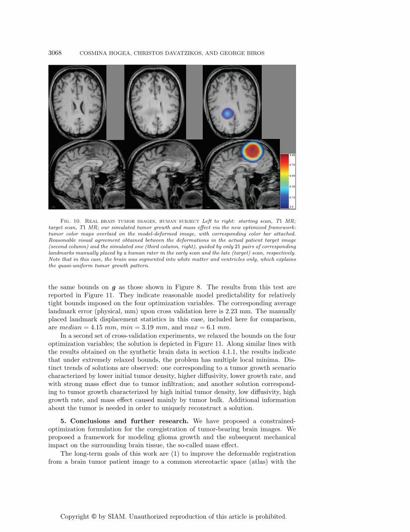
Fig. 10. Real brain tumor images, human subject Left to right: starting scan, T1 MR;target scan, T1 MR; our simulated tumor growth and mass effect via the new optimized framework:tumor color maps overlaid on the model-deformed image, with corresponding color bar attached.Reasonable visual agreement obtained between the deformations in the actual patient target image(second column) and the simulated one (third column, right), guided by only 21 pairs of correspondinglandmarks manually placed by a human rater in the early scan and the late (target) scan, respectively.Note that in this case, the brain was segmented into white matter and ventricles only, which explainsthe quasi-uniform tumor growth pattern.

the same bounds on g as those shown in Figure 8. The results from this test arereported in Figure 11. They indicate reasonable model predictability for relativelytight bounds imposed on the four optimization variables. The corresponding averagelandmark error (physical, mm) upon cross validation here is 2.23 mm. The manuallyplaced landmark displacement statistics in this case, included here for comparison,are median = 4.15 mm, min = 3.19 mm, and max = 6.1 mm.

In a second set of cross-validation experiments, we relaxed the bounds on the fouroptimization variables; the solution is depicted in Figure 11. Along similar lines withthe results obtained on the synthetic brain data in section 4.1.1, the results indicatethat under extremely relaxed bounds, the problem has multiple local minima. Dis-tinct trends of solutions are observed: one corresponding to a tumor growth scenariocharacterized by lower initial tumor density, higher diffusivity, lower growth rate, andwith strong mass effect due to tumor infiltration; and another solution correspond-ing to tumor growth characterized by high initial tumor density, low diffusivity, highgrowth rate, and mass effect caused mainly by tumor bulk. Additional informationabout the tumor is needed in order to uniquely reconstruct a solution.

5. Conclusions and further research. We have proposed a constrained-optimization formulation for the coregistration of tumor-bearing brain images. Weproposed a framework for modeling glioma growth and the subsequent mechanicalimpact on the surrounding brain tissue, the so-called mass effect.

The long-term goals of this work are (1) to improve the deformable registrationfrom a brain tumor patient image to a common stereotactic space (atlas) with the



Fig. 11. Cross validation. We report results from the leave-one-out cross-validation experi-ment for two cases, a first case (test 1) with tight bounds on the inversion parameters, and a secondcase (test 2) with relaxed bounds on the inversion parameters. The results for the first case indicatereasonable model predictability when tight bounds were imposed on g . The corresponding averagelandmark error (physical, mm) upon cross validation is 2.23 mm. These results for the second caseindicate that without tight constraints we obtain multiple local minima, which correspond to differenttumor growth physical scenarios.

ultimate purpose of building statistical atlases of tumor-bearing brains; and (2) toinvestigate predictive features for glioma growth after the model parameters are es-timated from given patient scans. The first is important for integrative statisticalanalysis of tumors in groups of patients and for surgical planning. The second isimportant for general treatment planning and prognosis.

We discussed numerical algorithms for solving the nonlinear systems of PDEs gov-erning the proposed unified model. The numerical solution procedure is designed tobe readily applied to 3D images of brain tumor subjects. These problems can result invery large deformations. To avoid remeshing, we have employed a structured grid dis-cretization. We illustrated the capabilities and flexibility of the method in capturingcomplex tumor shapes and the subsequent mass effect with reasonable computationalcost. We tested both the model and the automatic optimization framework on syn-thetic datasets and real brain tumor datasets and showed improvement compared toexisting approaches with less realistic models. (Of course, our model is still a veryrough approximation of true biophysics). In our numerical experiments, we observednonconvexity; one way to address it is by imposing strict lower and upper bounds.We are currently integrating the code with more complex similarity functions and



multiple imaging modalities.Overall the results are quite preliminary and inconclusive. The tumor model is

by no means predictive and quantitatively accurate. Our goal in this article is toshowcase an example in which several aspects of computational mathematics are usedin a practical setting. In the context of image registration for tumor-bearing images,a significant amount of additional work is necessary before one can draw conclusionson the clinical applicability of our approach.

First, we need to conduct sensitivity analysis of the solution with respect to seg-mentation and elastic material properties of the brain and the tumor tissues. Second,we need to have more general parametrizations for the initial profile of the tumor.In fact, one should not invert for the initial conditions, but rather for a forcing term(with compact support, in time) that models the initial occurrence of tumor, whichin general takes place in an unknown moment in time. The current optimizationsolver is robust, but slow; we require hundreds of function evaluations, and this willbe a significant bottleneck as we introduce more optimization variables. For exam-ple, in our formulation we considered a single-degree-of-freedom parametrization ofthe initial tumor concentration; richer representations are necessary for batch pro-cessing of images. We are currently implementing fast PDE-constrained optimizationalgorithms.

From a practical point of view, serial scans of human subjects with gliomas pro-gressing into higher malignancy are rare, although some clinical studies have beenconducted [39]. Instead, animal experiments are necessary to construct more phys-iologically correct models. Such datasets can be employed in conjunction with ourproposed framework for a preliminary validation/calibration of our image registra-tion framework. Most important, rich longitudinal datasets will enable incorporationand validation of more sophisticated tumor models that include diffusive anisotropy,edema, necrosis, angiogenesis, and chemotaxis.

REFERENCES

[1] E. C. Alvord, Jr., and C. M. Shaw, Neoplasms affecting the nervous system of the elderly,in The Pathology of the Aging Human Nervous System, S. Duckett, ed., Lea and Febiger,Philadelphia, 1991.

[2] P. Angot, H. Lomenede, and I. Ramiere, A general fictitious domain method with non-conforming structured meshes, in Proceedings of the International Symposium on FiniteVolumes IV, Hermes Science, Cachan, France, 2005, pp. 261–272.

[3] R. Araujo and D. McElwain, A history of the study of tumor growth: The contribution ofmathematical modeling, Bull. Math. Biol., 66 (2004), pp. 1039–1091.

[4] R. P. Araujo and D. L. S. McElwain, A mixture theory for the genesis of residual stressesin growing tissues I: A general formulation, J. Appl. Math., 65 (2005), pp. 1261–1284.

[5] J. Ashburner, J. Csernansky, C. Davatzikos, N. Fox, G. Frisoni, and P. Thompson,Computer-assisted imaging to assess brain structure in healthy and diseased brains, TheLancet (Neurology), 2 (2003), pp. 79–88.

[6] R. Bajcsy, R. Lieberson, and M. Reivich, A computerized system for the elastic matching ofdeformed radiographic images to idealized atlas images, J. Comput. Assisted Tomography,7 (1983), pp. 618–625.

[7] S. Balay, K. Buschelman, L. Dalcin, V. Eijkhout, W. D. Gropp, D. Karpeev,

D. Kaushik, M. Knepley, L. C. McInnes, B. F. Smith, and H. Zhang, PETSc homepage, http://www.mcs.anl.gov/petsc (2007).

[8] M. F. Beg, M. Miller, A. Trouve, and L. Younes, The Euler-Lagrange equation for interpo-lating sequence of landmark datasets, in Medical Image Computing and Computer-AssistedIntervention (Miccai 2003), Pt. 2, Lecture Notes in Comput. Sci. 2879, Springer-Verlag,Berlin, 2003, pp. 918–925.

[9] G. Biros and O. Ghattas, Parallel Lagrange–Newton–Krylov–Schur methods for PDE-constrained optimization. Part I: The Krylov-Schur solver, SIAM J. Sci. Comput., 27(2005), pp. 687–713.



[10] H. M. Byrne, J. R. King, D. L. S. McElwain, and L. Preziosi, A two-phase model of solidtumor growth, Appl. Math. Lett., 16 (2002), pp. 567–573.

[11] G. E. Christensen, S. Joshi, and M. Miller, Volumetric transformation of brain anatomy,IEEE Trans. Med. Imaging, 16 (1997), pp. 864–877.

[12] O. Clatz, M. Sermesant, P.-Y. Bondiau, H. Delingette, S. K. Warfield, G. Malandain,

and N. Ayache, Realistic simulation of the 3D growth of brain tumors in MR imagescoupling diffusion with mass effect, IEEE Trans. Med. Imaging, 24 (2005), pp. 1334–1346.

[13] D. L. Collins, P. Neelin, T. M. Peters, and A. C. Evans, Automatic 3D intersubjectregistration of MR volumetric data in standardized Talairach space, J. Comput. AssistedTomography, 18 (1994), pp. 192–205.

[14] V. Cristini and J. Lowengrub, Nonlinear simulation of tumor growth, J. Math. Biol., 46(2003), pp. 191–224.

[15] M. B. Cuadra, C. Pollo, A. Bardera, O. Cuisenaire, J.-G. Villemure, and J.-P. Thiran,Atlas-based segmentation of pathological MR brain images using a model of lesion growth,IEEE Trans. Med. Imaging, 23 (2004), pp. 1301–1314.

[16] C. Davatzikos, D. Shen, A. Mohamed, and S. K. Kyriacou, A framework for predictivemodeling of anatomical deformations, IEEE Trans. Med. Imaging, 20 (2001), pp. 836–843.

[17] S. Del Pino and O. Pironneau, A fictitious domain based general PDE solver, in NumericalMethods for Scientific Computing, Proceedings of the Conference METSO-ECCOMAS, E.Heikkola, ed., CIMNE, Barcelona, 2003.

[18] J. C. Gee, D. R. Haynor, L. LeBriquer, and R. K. Bajcsy, Advances in elastic matchingtheory and its implementation, in Proceedings of the First Joint Conference on ComputerVision, Virtual Reality and Robotics in Medicine and Medial Robotics and Computer-Assisted Surgery (CVRMED-MRCAS ’97), Lecture Notes in Comput. Sci. 1205, 1997,pp. 63–72.

[19] A. Gefen and S. S. Margulies, Are in vivo and in situ brain tissues mechanically similar?,J. Biomechanics, 37 (2004), pp. 1339–1352.

[20] A. Giese and M. Westphal, Glioma invasion in the central nervous system, Neurosurgery,39 (1996), pp. 235–250.

[21] R. Glowinski, T. W. Pan, R. O. Wells, and X. D. Zhou, Wavelet and finite elementsolutions for the Neumann problem using fictitious domains, J. Comput. Phys., 126 (1996),pp. 40–51.

[22] G. A. Gray and T. G. Kolda, Algorithm 856: APPSPACK 4.0: Asynchronous parallel patternsearch for derivative-free optimization, ACM Trans. Math. Software, 32 (2006), PP. 485–507.

[23] M. Gurtin, An Introduction to Continuum Mechanics, Academic Press, New York, 1981.[24] S. Habib, C. Molina-Paris, and T. Deisboeck, Complex dynamics of tumors: Modeling an

emerging brain tumor system with coupled reaction-diffusion equations, Phys. A Statist.Mech. Appl., 327 (2003), pp. 501–524.

[25] A. Hagemann, K. Rohr, H. Stiehl, U. Spetzger, and J. Gilsbach, Biomechanical modelingof the human head for physically based, nonrigid image registration, IEEE Trans. Med.Imaging, 18 (1999), pp. 875–884.

[26] C. Hogea, G. Biros, and C. Davatzikos, Fast Solvers for Soft Tissue Simulationwith Application to Construction of Brain Tumor Atlases, Tech. report ms-cis-07-04,www.seas.upenn.edu/∼biros/papers/brain06.pdf (2006).

[27] C. Hogea, F. Abraham, G. Biros, and C. Davatzikos, Fast solvers for soft tissue simulationwith application to construction of brain tumor atlases, submitted.

[28] C. Hogea, F. Abraham, G. Biros, and C. Davatzikos, A framework for soft tissue simula-tions with applications to modeling brain tumor mass-effect in 3d images, in Proceedings ofthe Medical Image Computing and Computer-Assisted Intervention Workshop on Biome-chanics, Copenhagen, 2006.

[29] C. Hogea, G. Biros, F. Abraham, and C. Davatzikos, A robust framework for soft tissuesimulations with application to modeling brain tumor mass effect in 3D MR images, Phys.Med. Biol., 52 (2007), pp. 6893–6908.

[30] C. Hogea, G. Biros, and C. Davatzikos, An image-driven parameter estimation problem fora reaction-diffusion glioma growth model with mass effects, submitted.

[31] C. Hogea, G. Biros, and C. Davatzikos, A coupled diffusion-elasticity PDE-constrainedframework for simulating gliomas growth: A medical imaging perspective, presented at theSIAM Conference on Computational Science and Engineering (Costa Mesa, CA), 2007.

[32] C. Hogea, C. Davatzikos, and G. Biros, An image-driven parameter estimation problemfor a reaction-diffusion glioma growth model with mass effects, J. Math. Biol., 56 (2008),pp. 793–825.



[33] Z. Hu, D. Metaxas, and L. Axel, In vivo strain and stress estimation of the heart left andright ventricles from mri images, Med. Image Anal., 7 (2003), pp. 435–444.

[34] A. R. Kansal, S. Torquato, G. Harsh IV, E. Chiocca, and T. Deisboeck, Simulated braintumor growth dynamics using a three-dimensional cellular automaton, J. Theoret. Biol.,203 (2000), pp. 367–382.

[35] T. G. Kolda et al., APPSPACK home page, http://software.sandia.gov/appspack/version5.0.1(2007).

[36] T. G. Kolda, Revisiting asynchronous parallel pattern search for nonlinear optimization, SIAMJ. Optim., 16 (2005), pp. 563–586.

[37] S. Kyriacou, C. Davatzikos, S. Zinreich, and R. Bryan, Nonlinear elastic registrationof brain images with tumor pathology using a biomechanical model, IEEE Trans. Med.Imaging, 18 (1999), pp. 580–592.

[38] K. E. Lunn, K. D. Paulsen, D. R. Lynch, D. W. Roberts, F. E. Kennedy, and A. Hartov,Assimilating intraoperative data with brain shift modeling using the adjoint equations,Med. Image Anal., 9 (2005), pp. 281–293.

[39] E. Mandonnet, J. Delattre, M. Tanguy, K. Swanson, A. Carpentier, H. Duffau,

P. Cornu, R. Van Effenterre, E. Alvord, Jr., and L. Capelle, Continuous growthof mean tumor diameter in a subset of grade II gliomas, Annals of Neurology, 53 (2003),pp. 524–528.

[40] M. I. Miga, K. D. Paulsen, J. M. Lemery, S. D. Eisner, A. Hartov, F. E. Kennedy, and

D. W. Roberts, Model-updated image guidance: Initial clinical experiences with gravity-induced brain deformation, IEEE Trans. Med. Imaging, 18 (1999), pp. 866–874.

[41] K. Miller and K. Chinzei, Mechanical properties of brain tissue in tension, J. Biomech., 35(2002), pp. 483–490.

[42] K. Miller, K. Chinzei, G. Orssengo, and P. Bednarz, Mechanical properties of brain tissuein-vivo: Experiment and computer simulation, J. Biomech., 33 (2000), pp. 1369–1376.

[43] M. I. Miller, A. Trouve, and L. Younes, On the metrics and Euler-Lagrange equations ofcomputational anatomy, Ann. Rev. Biomed. Engrg., 4 (2002), pp. 375–405.

[44] J. Modersitzki, Numerical Methods for Image Registration, Oxford University Press, Oxford,UK, 2001.

[45] A. Mohamed, Combining Statistical and Biomechanical Models for Estimation of AnatomicalDeformations, Ph.D. thesis, Johns Hopkins University, Baltimore, MD, 2006.

[46] A. Mohamed and C. Davatzikos, Finite element modeling of brain tumor mass-effect from3d medical images, in Proceedings of Medical Image Computing and Computer-AssistedIntervention, Palm Springs, 2005 pp. 400–408.

[47] S. Osher and R. Fedkiw, Level Set Methods and Dynamic Implicit Surfaces, Springer, NewYork, 2003.

[48] X. Papademetris, A. J. Sinusas, D. P. Dione, R. T. Constable, and J. S. Duncan, Estima-tion of 3-D left ventricular deformation from medical images using biomechanical models,IEEE Trans. Med. Imaging, 21 (2002), pp. 786–800.

[49] P. Roache, Computational Fluid Dynamics, Hermosa, Albuquerque, NM, 1972.[50] K. R. Swanson, E. C. Alvord, and J. D. Murray, A quantitative model for differential

motility of gliomas in grey and white matter, Cell Proliferation, 33 (2000), pp. 317–329.[51] K. R. Swanson, C. Bridge, J. D. Murray, and E. C. Alvord, Virtual and real brain tumors:

Using mathematical modeling to quantify glioma growth and invasion, J. Neurolog. Sci.,216 (2003), pp. 1–10.

[52] P. Tracqui and M. Mendjeli, Modelling three-dimensional growth of brain tumors from timeseries of scans, Math. Models Methods Appl. Sci., 9 (1999), pp. 581–598.

[53] R. Tyson, L. Stern, and R. LeVeque, Fractional step methods applied to a chemotaxis model,J. Math. Biol., 41 (2000), pp. 455–475.

[54] J. Verwer, W. Hundsdorfer, and J. Blom, Numerical Time Integration for Air Pol-lution Models, Tech. report MAS-R9825, CWI, Amsterdam, 1991. Available online athttp://ftp.cwi.nl/CWIreports/MAS/MAS-R9825.pdf.

[55] S. K. Warfield, F. Talos, A. Tei, A. Bharatha, A. Nabavi, M. Ferrant, P. Black,

F. Jokesz, and R. Kikinis, Real-time registration of volumetic brain MRI by biomechan-ical simulation of deformation during image guided neurosurgery, Comput. Visual. Sci., 5(2002), pp. 3–11.

[56] R. M. Wasserman, R. S. Acharya, C. Sibata, and K. H. Shin, Patient-specific tumor prog-nosis prediction via multimodality imaging, Proc. SPIE Int. Soc. Opt. Eng., 2709 (1996),pp. 468–479.

[57] S. Zhu, G. Yuan, and W. Sun, Convergence and stability of explicit/implicit schemes forparabolic equations with discontinuous coefficients, Internat. J. Numer. Anal. Model., 1(2004), pp. 131–145.

Documents

Brain-Tumor Interaction Biophysical Models for Medical Image