Embed Size (px)
Citation preview

BPF ± 4 BPF
LO,
LINT))IT CORPORATION10453 Ros.11e StreetSan Dioqo, CA 92121
KR~ltR CONTROJL CODING RAXVDOKQUD
SM~z'.. ________RE-PORT)
PHA SE LOCKED M~5 zLOOP
REF MUJLTIPLIEU -
+2 FILTER/ -
-AMP
QUAD FILTER/A
A ELECTEr
70MHz P7MzTx OUTPUT
it W, /A COM LINKABIT, INC.j~t 1 'II 3033 Sc~erc, -c.
Son D~efo. CA ,2,12!61Q,1457 2312
WU kJ FILL y 8 9o 16a
3EOJ.4zt 3xi< 0cU:)dAUIAy

0*
LINKABIT CORPORATION10453 Roselle StreetSan Diego, CA 92121
3 ERROR CONTROL CODING HANDBOOK S
(FINAL REPORT)
Joseph P. Odenwalder
j. DTIC15 Jy 1976 E ECT
•: JUL3 3
Prepared Under Contract No. F44620-76-C-0056
* for
"Issistant Chief of Staff, Studies and AnalysisCommand, Control and Reconnaissatnce Division
Strategic DirectorateHq. United States Air Force
* A revised and updated version of much of thematerial in this report is available in
: J.P. Odenwalder, "Error Control," inData Communications, Networks, and Systems,T.C. 3artee, Ed. Indianipolis, IN: -
Howard Sams, 1985, Chapter 10.P

TABLE OF CONTENTS
Section Pace
1.0. Introduction .... .............. 1 S
2.0 Summary of the Procedures for Specifying ErrorControl Codes .d. ...................... 4
2.1 Error Correction Versus Error Dectection . 5
2.2 Block Versus Convolutional Codes ... ..... 7
2.3 Summary of the Performance of Forward
Error Correcting Coding Systems .......... 9
2.4 Code Specification ..... ............ . 13
3.0 Potential Advantages of Coding ..... ......... 15
- 3.1 I'ncoded System Error Rate Performance . . 15
3.1.1 Additive White Gaussian NoiseChannel . ............ 15
3.1.1.1 Coherent Phase-ShiftKeyed Systems........ .. 15
3.1.1.2 Differentially CoherentPhase-Shift KeyedSystems . ....... 19
3.1.1.3 Noncoherently Demo-dulated Orthogonal SignalModulated (MFSK) Systems 22
3.1.2 Independent Rayleigh FadingChannel. . . . . . . . . . . . 24
3.1.3 Summary of Uncoded SystemPerformance ............ ... 28
3.2 Channel Capacity and Other FundamentalLimits to Coding Performance. . . . . 30
3.2.1 Binary Symmetric Channels. . .. 31
3.2.2 Additive White Gaussian NoiseChannel .... ............. .... 38
3.2.2.1 BPSK or QPSK :m:odulation. 38
-ii-

I A
Section Page
3.2.2.2 M-ary PSK Modulation .45
3.2.2.3 D3PSK Modulation . . .49
3.2.2.4 Honcoherently Demo-dulated MFSK ......... 54
3.2.3 Lndependent Rayleigh Fading
Channel ....... ............. s7
4.0 Block Codes . . . . . . . . . ........ 60
4.1. Nazming Codes . . . . . . . . . ... . 68
4.2 Extended Golay Code . ............ 74
4.3 BCH Codes . . . . . . .......... 81
4.4 Reed-Solomon Codes . . . . . . . . . .. 86
5.0 Binary Convolutional Codes . . ......... 93
5.1 Viterbi Decoded Convolutional Codes . . 201
5.1.1 The Viterbi Decoding Algorithmfor the Binary Symmetric Channel-10l
5.1.2 Distance Properties of Con-volutional Codes ........ 105
5.1.3 Generalization of Viterbi De-coding te Arbitrary Rate Con-volutional Codes. . . . . . . . 106
5.1.4 Systematic and Nonsystematic,CO. Convolutional Codes . . . . . . 71ll
cr 5.1.5 Catastrophic Error Propagation . 113
"5.1.6 Generalization of viý-erbiDecoding to Soft QuantizationChannels. .. ...... ............. 117
5.1.7 Path Memory Truncation .... 113
5.1.8 Code Selection...... .. .. .. . 1..120
5.1.9 Computer Simulation Performance| Results ................ ... 122fist.
1 5.1.10 Analytical Performance Tech-niques with No Quantimzrion. 134
-iii-
0I
_ o0• _,, 0 • 0 0• ' *

0
2-
Section page
5.1.11 Analytical PerformanceTechniques with Quantization . 143
5.1.12 Node Synchronization and PhaseAmbiguity Resolution ... ...... 151'
5.1.13 Quantization Threshold Levels . 155
5.1.14 Implementation Considerations . 156
S5' Sequential Decoded Convolutional Codes . 161
5.2.1 Code Selection . . . . . . . .. 167
5.2.2 Performance Results . . . . . . 167
5.2.3 Implementation and ApplicationConsiderations . . . . . . . . . 174
5.3 Feedback Decoded Convolutional Codes 176
5,3.1 Code Selection .............. 178
5.3.2 Performance Results . . . . . . 178
5.3.3 Implementation and ApplicationConsiderations .......... .... 180
6.0 Nonbinary Modulation Convolutional Codes . . . 183
7.0 Concatenated Codes . . . . 0 ............ . 191
7.1 Viterbi-Decoded Convolutional InnerCode and Reed-Solomon Outer Code . . . . 191
7.2 Viterbi-Decoded Convolutional Inner Code ',
and Feedback-Decoded Convolutional OuterCode . . . . . . . ................ 199
Appendix A. Glossary of Coding Terminology .... ... 202
Appendix B. Glossary of Symbols ............. .. 209
REFERENCES ............. .................... ... 210
-iv-
0 0 0 _S 0

TABLE OF FIGURES
Figure Pg
3.1 Bit er-or probability versus E /IN per-formance of coherent BPSK, QPSk, Ind octal-PSK . . . . . . . . . #. . . . . . . .. . . .. . 17
3.2 Modem input symbol-to-channel phase mappingfor QPSK and octal-PSK. . . . . ......... 18
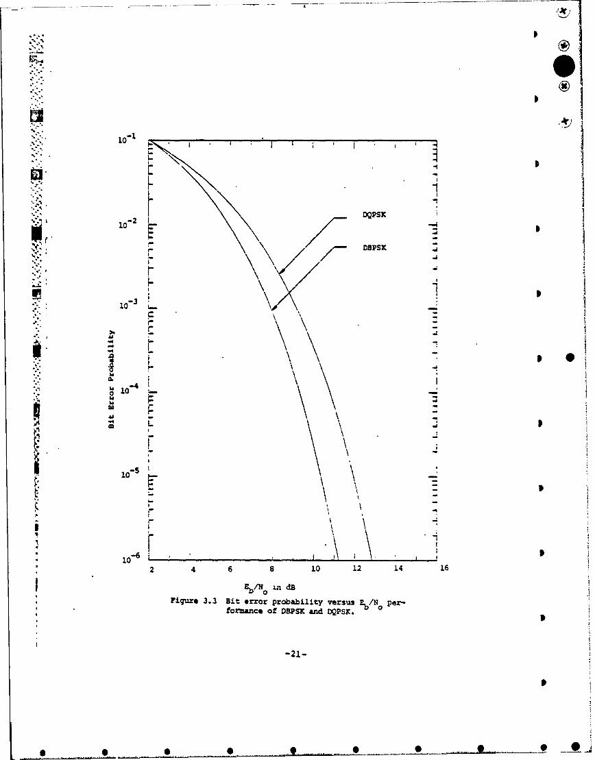
3.3 Bit error probability versus Eb/No per-fozmance of DBPSK and DQPSK .............. ... 21
3.4 Bit error probability versus E/NO performanceof binary and 8-ary MSK. . . . . . ....... 25
3.5 Bit error probability versus E,%/1 performanceof binary FSK on a Rayleigh fading channel forseveral orders of diversity. . ......... 27
3.6 Binary symmetric channel transition diagram 32
3.7 Coding limits for a binary symaietric channel.. 34
3.8 Block diagram of a coding system with inter-leaving/deinterleaving. . . . . . .............. 36
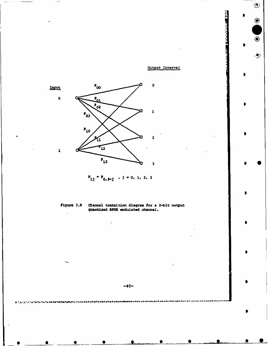
3.9 Channel transition diagram for a 2-bit outputquantized EPSK modulated channel. .. . . . . 40
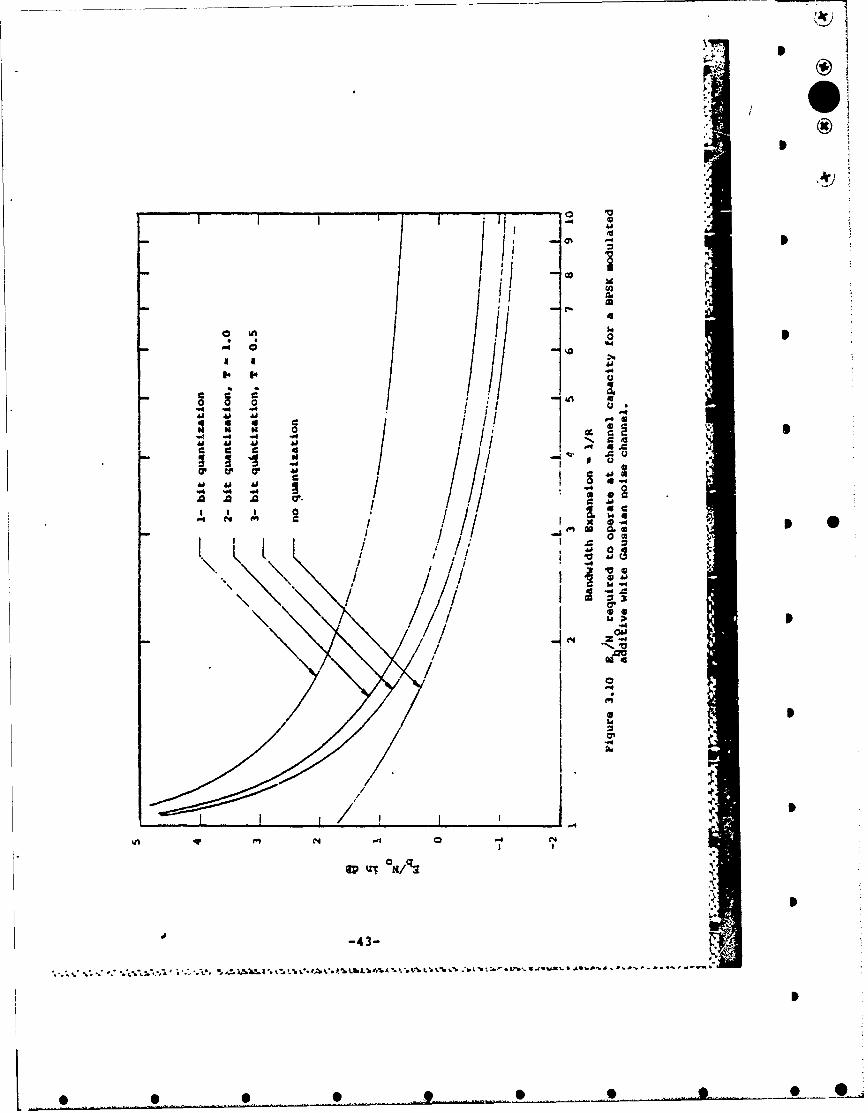
3.10 EWN_ required to operate at channel capacityf r ?or a SPSK modulated additive white Gaussiannoise channel. . . . . . . . . 43
3.11 EI/N require to operate at R-R for a BPSKm~du 2ated additive white Gaussiin noise channel. 44
3.12 /N required to operate at R-R versus the un-ckdea OPSK bandwidth expansion fSr =ctal-PSK andQPSK with no quantization. . .......... 47
3.13 Diagrams of the first quadrant signal spDacequantization intervals for two possible 6-bitquantization techniques for octal-BSK .... 48
34 ,/N required to operate at R-R for ani1tegleaved DBPSK channel. ........ ...... 51
3.15 Potential coding gain of rate 1/2 coding withBPSK and DBPSK modulation and 3-bit quan-tization .............. ................... 53
• + O ..... . . ... . ... .. .. •i ...+ , + . + + - " - + •
*
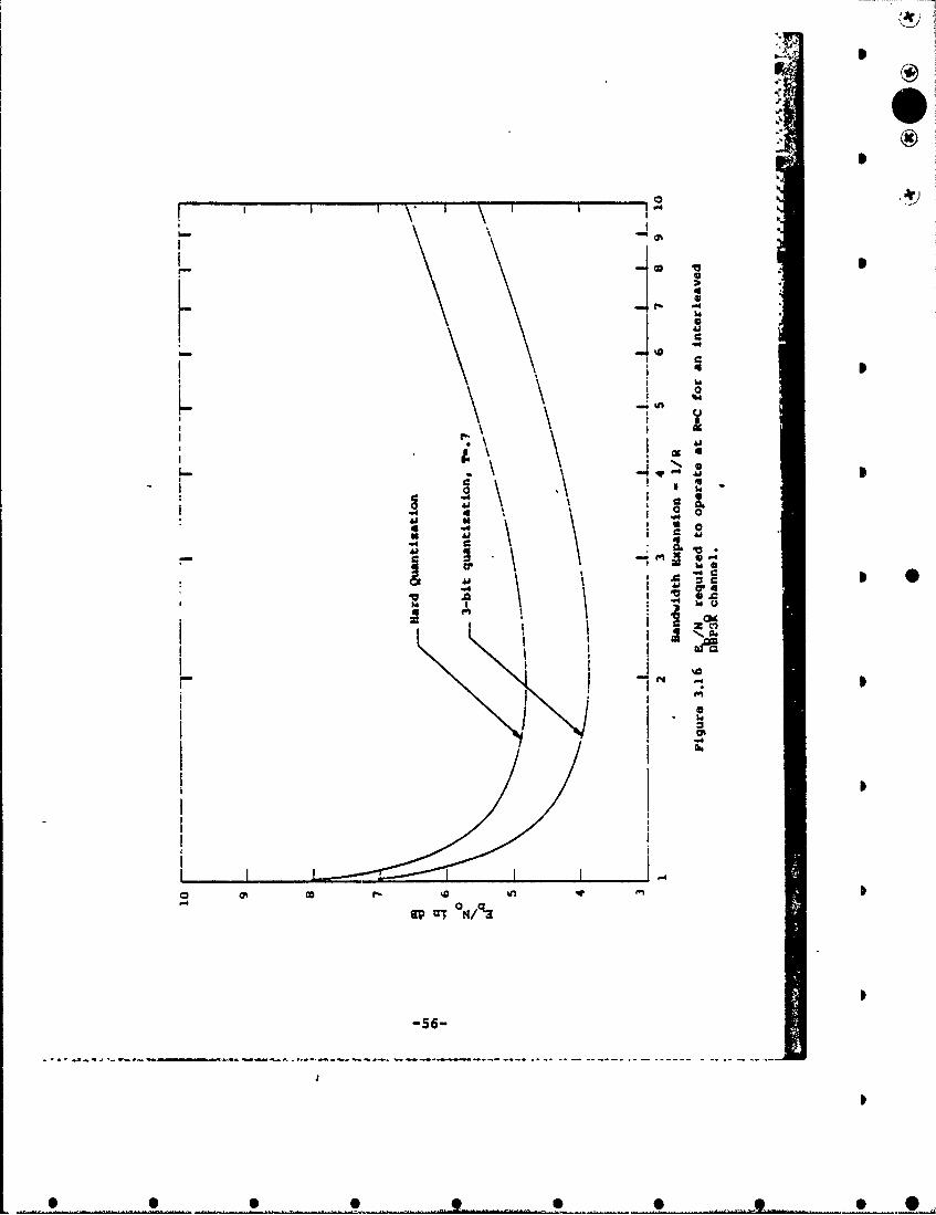
3.16 5,/: required to operate at R=C for aniItehleaved DBPSK channel ...... ... 56
Z.17 E%/N required to operate at R=R for an indepen-d nt Rayleigh fading channel witR MSK. . . . 59
4.1 Block error probability versus channel errorprobability for block length n-2m - 1 Hammingcodes with mn3, 4, and 5 ............ ... 71
4.2 Bit error probability versus charnel merror probability for block length n-2 -1Hamming codes with m-3,4, and 5 .... ....... 72
4.3 Probability of an undetected error versuschannel error probability for block lengthn_2 -1 Hamming codes with m-3, 4, and 5. 73
4.4 Bit error arobability versus E•/N fo: blocklength n-2 --I Haing codes wi h g3, 4, and5 on a AWGN channel. . . . . . . . . . . . . 75
4.5 Block, bit and undetected error probabilitissversus channel error rate with extended Golaycoding. . ................. 3Q 0
4.6 Block, bit and undetected error probabilitiesversus k/N for BPSK or QPSK modulation, anAWGN c1%.uaQJ., and extended Golay coding. . . 92
4.7 Bit error probability versus channel errorrate performance of sev*'ral block length 127,BCH codes. . . . . . . . . . . . . . . . . . 87
4.8 Bit error probability versus channel symbolerror probability for 32-orthogonal-signalmodulation and n-31, E-error-correctingReed-Solomon coding. o . . . . . . . . .. 91
4.9 Bit error probability versus EI/N perform-ance of several n-31, E-error- or ectingReed-Solomon coding systems with 32-aryMFSK modulation on an AWGN channel ........ ... 92
5.1 Rate b/v, constraint length K convolutionalencoder. ....... ................... ... 94 0
5.2 Rate 1/2 constraint length 3 convolutionalencoder ........ ................... .... 95
5.3 Tree code representation for coder ofFigure 5.2 ...... ................. .... 97
-vi-
I
* 0 _ 6 ___

Figure 2 ae
' 5.i Trellis code representation for coder ofFigure 5.2. ............... . . 99
5.5 State-diagram representation for coder 0of Figure 5.2. . ......... . . . . . 100
5.6 Trellis diagram labelled with distancesfrom the all zeros path. . . . . . . . . . 107
5.7 1-4, R-2/3 encoder. . . . . . . . . . . . . 109
5.8 State diagram for code of Figure 5.7. . . . 110
5.9 Systematic convolutional encoder forX-3, R-1/2............ . . . . . . . . .112
5.10 Coder displaying catastrophic errorpropagation ................ 115
5.11 Bit error- probability versus L.I/N per-formance of a 1-7, R-1/2 convonudonalcoding system with EPSK modulation and anAtGN channel. . . . . . . . . . . . . . . . 124
5.12 Bit error probability versus / N per-formance of a K-7, R-1/3 convolutlonalcoding system with PA'jodulation and anAWGN channel. .... ' . . ........ 125
5.13 Bit error probability ve X per-fo'mance of a K-9, R-3/4 convol. al ?coding system with EPSI modulatiOz d anAWGN channel. . . . . . . . . . . . . . . . 126
5.14 Coding gain for several convolutional cOtswith BPSK modulation, AWGN, and 3-bitreceiver quantization . . . . . . . . . 128
5.15 Bit error probability versus channel error Irate performance of several convolutionalcoding system• . .. .o. .. ...... 129 !
5.16 Performance of tlhie modulation and codingsystem with a rate 2/3, constraint length8, Viterbi-decoded convolutional code and 0an octal-PSK modem for several path lengthmemories. .. . . . . . . . . . .. . . . 131
5.17 Bit error probab.lity versus Eb/N per-formance of a K-7, R-1/2 convolut~onalcoding system with DBPSK modulation and anAWGN channel. . . . . . . . . . . . . . . . 133 0
-vii-

-~ U
SOI
f' .ure ag
5.18 Modified state diagram for the K-3, R-1/2convoiutional code of Figure 5.2 ..... .. 139
5.19 Bit error probability versus Eb/N perfor-mance bouises for several R-1/2 Viaerbi-decoded convolucional coding systemswith no quantization ..... ............ ... 144
5.20 Bit error probability versus Eb/N1 perfor-mance bounds for several R-1/3 ViWerbi-decoded convolutional coding systems withno quantization. . . . . ............ 145
5.21 Bit error pri)ability versus .b/N perfor-mance bound: fr several R-1/4 Viierbi-decoded conv'.,3tional coding systemswith r quantization. ................... .. 146
5.22 Bit error probability versus E£/N per-formance bounds fer several R-"/3 0 Viterbi-lecoded convolutional coding systems with noqua:itzation ........................ 147
5.2 Bit error proba.bility versus Sb/NN perfor-mar :e k-unds foz several R-3/4 Vi~erbi-dewoJ"ýd ,3nvolutional ccling systems with
S;uant-,:at 4orn. . . . . . . . . . . . . . . 148
5.24 Zrc=:ar I, ; • /No required to maintain a2 X 10":i error rate v•rsis error inAGC mee !-ý ment of for a K-7, R-1/2code . . . . . . . . . . . . . . . . . . . . . !-57
5.25 Pareto exponent versus E/N for an AWGNc- nel with 3-bit (T.587 qeantization ... .
5.26 Pareto evponent versus Zb/NI for an AWGNchannel qith hard quantizatlon ............ 166
5.27 Probability of a failure to decode a 1000-information-bit frame for a KX24, R-1/2sequential decoder with 3-bit quantization(Simulation) ........ ................. .. 169
5.28 Probability of a failure to decode a 1000-information-bit frame for a K-24, R=1/2sequential decoder with hard quantization,Simulation) .............. ................. 10
€,p

Figure Pace
* ®~
5.29 Bit error rate due to alternate decodingof 1000-information-bit frames not decodedin 50 ms for a K-24, R-1/2, non-systematicsequential decoded convolutional codingsystem (Simulation). . .. .... .... 172
5.30 Bit error rate versus channel errorrate performance of several conmerciallyavailable feedback-decoded convolutionalcoding systems. . . . . . . . ............... 179
5.31 Message error probability versuschannel error rate for a K-10, L-11, R-1/2feedback-decoded convolutional codingsystem. . . . . . . . . . . . . . . . . . . 181
6.1 Rate 1/2 dual-3 convolutional encoder. . . 184
6.2 Finite field representation of a rate I/vdual-k convolutional encoder ......... ... 185
6.3 Performance of a R-1/2, dual-3 convolu-tional coding systera with noncoherentlydemodulated 8-ary MFSK on an independent I •Rayleigh fading channel with no quanti-z a t i o n . . . . . . .... 1 8 9
7.1 Block diagram of a concatenAted codingsystem. . . . . . ... . 192
7.2 Concatenated code bit e:ror probabilityperformance with a K-7, R-1/2 con-volutional inner code and an 8-bit/symbolR-S outer code . . . . . . . . . . . . . 195
7.3 Sumrary of concatenated coding bit errorprobabilit-y performance with a K-7, R-1/2convolutional inner code and various R-Souter codes. . . . . . . . . . ....... 197
7.4 Concatenated code block error probabilityperformance with a K=7, R=1/2 convolutionalinner code and an 8 bit/symbol R-S outercode. . . ..... .. . .. ... . ................. 198
7.5 Performance of a concatenated codingsystem with a K-7, R-1/3 Viterbi-decodedconvolutional inner code and a K-8, R-3/4distance 5 feedback-decoded convolutionalouter code ........ ................ ... 200
-ix-
____• S .. • 0a

TABLE OF TABLES
Table Pace
2.1 Summary of the Eb/NO requirements of severalcoded communication systems for a bit errorrate of 10-5 with BPSK modulation ......... 11
2.2 Summary of t'.e R./N requirements and codinggains of K-7, R-•/2°Viterbi-decoded convolu-tional coding systems with several modulationtypes at a bit error rate of I10-.. . . . . . 12
3.1 Summary of uncoded system performance. . . 29
4.1 Summary of the ZI/N ratios required toachieve a 10-l bRt Srror probability withHnmming coding for several modulation/demodulation techniques .... ........... 76
4.2 Weighd enumerator and 0 coefficients for theextended Golay code (12f. .... . . .. . _.9
4.3 E IN required to achieve a 10-5 bit errorrAteOwith extended Golay coding and severalmodulation/demodulation techniques .... 33
5.1 Comparison of systematic and nonsystematicR-1/2 code distr.ces.. . . . . . . ....... 114
5.2 Optimum short con.%traint length R-1/2 and1/3 convolutional codes. . . . ......... 121
5.3 Error Burst statistics for a K-7, R- 1/2 systemwith 3-bit quantization. . . . . . . . . . . 135
5.4 Error burst statistics for a K-7, R-1/2 systemwith hard quantization ...... .............. 1&'6
5.5 Upper bound coefficients of (5.6) and (5.7).. 15:25.6 Measured performance of LS 4816 convolutional
encoder-sequential decoder with data rate=50Kbps, packet size-1000 bits, constraint and taillength=48, code rate=l/2, and undetectederror rate <10- 6. . . . .. . . . . . . . .. . . . . . . . .. 173
I

TABLE OF FIGURES AND TABLES THAT PROVIDE PERFORI•CE
RESULTS FOR UNCODED SYSTEMS
Figure ELM
3.1 Bit error probability versus E6/N per-formance of coherent BPS_, QPSX, indoctal-PSK . . . . . .. . ........ 17
3.3 Bit error probability versus Eb/No per- 21formance of DPBSK and CQPSK ...... 21
3.4 Bit error probability versusperformance of binary and 8-ary MSK.. 25
3.5 Bit error probability versus !%N per-formance of binary FSK on a Rayleighfading channel for several orders ofdiversity . .............. .. 27 0 0
Table
3.1 Summary of uncoded system performance.. 29 6
D
*D
• •• ••IP... ,... •• - 3

A TABLE OF -IGURES AND TABLE THAT PROVIDE PERFORMANCE
RESULTS FOR HAMMING CODING SYSTEMS
Figure Page
4.1 Block error probability versus channelmerror probability for blcck length n-2m--Hamming codes with m-3, 4, and 5 . . . . 71
4.2 Bit error probability versus channel merror probability for block length na2 -1Haming codes with m-3,4, and 5. . . . . 72
4.3 Probability of an undetected error versuschapnel error probability for block lengthnW2 -1 Hamming codes with m-3, 4 and 5. 7
4.4 Bit error probability versus F•/N forblock length ri2 -i Hamming co~es withm-3, 4, and 5 on a AWGN channel. ..... 75 •
Table Page
4.1 Sumary of the E5/N ratios required toachieve ai 10 - b t error probability withHamming coding for several modulation/demodulation techniques. . . . . . .... 76
I
-xii-
0

"TABLE OF FIGURES AND TABLES THAT PROVIDE PERFORMANCE
RESULTS FOR GOLAY CODING SYSTEMS
Figure Paga
4.5 Block, bit and undetected error prob- Sabilities versus channel error ratewith extended Golay coding . . . . • 80
4.6 Block, bit and undetected error prob-abilities versus E/IN for BPSK 01 OPSKmodulation, an AWGN cnannel, and extendedGolay coding.......... . . .. . . 82
%m ,
Table Page
4.3 /N required to achieve a 10s bit errorr teowith extended Golay coding and severalmodulation/demnodulation techniques . . . . 83 I
I'..
m,,
..S
• °..I
L..
"%*.I
__.'iii
,,*.'I
_ _ ~o
TABLE OF FIGURES AND TABLES THAT PROVIDE PERFORMANCE
"RESULTS FOR BCH CODING SYSTEMS
Figuire Page
4.7 Bit error probability versus channel errorrate performance of several block length"127, BCH codes...... . . . . . . . . . . 87
F.4.
°,'.
-xiv-
D
O .. .. . . .. o_ . . . . .0.. . . .. .... .. .. ... 0+ .. . .,• . . . _ . ..O

TABLE OF FIGURES AND TABLES THAT PROVIDE PERFORMANCE
RESULTS FOR REED-SOLOMON CODING SYSTEMS
-p
!
_e___ Page
I p
4.8 Bit error probability versus channelsymbol error probability for 32-orthogonal-
.1 signal modulation and n-31, E-error-cor-recting Reed-Solomon coding . . . . . .91
4.9 Bit error probability versus E/N per-formance of several n-31, E-er or-correcting"Reed-Solomon coding systems with 32-aryMFSK modulation on an AWGN channel . . . . 92
I,
: * 02I
I p
9
I!
I
I
!p
tp
I -xv-
p
9 • ..... *.. ... ... e •S
S
TABLE OF FIGURES AND TABLES THAT PROVIDE PERFORMANCE
RESULTS FOR VITERBI-DECODED CONVOLUTIOZIAL
CODING SYSTEMS S
3 ,
5.11 Bit error probability versus E./N per-formance of a K-7, R-l/2 convo utonalcoding system with BPSK modulation andan AWGN channel. . . . . . . . . . . . 124
5.12 Bit error probability versus E,/N_ per-formance of a K-7, R-1/3 convoTudoncoding system with BPSK modulation and an 5AWGN channel. . . . . . . . . . . . . . 125
5.13 Bit error probability versus Ek/N per-formance of a K-9, R-3/4 convolut.onalcoding system with BPSK modulation and 126an AWGN channel . . . . . . . . . . . . .
5.14 Coding gain for several convoltuional codeswith BPSK modulation, AWGN, and 3-bit 128receiver quantization . . . . . . ....
5.15 Bit error probability versus channel errorrate performance of several convolutionalcoding systems. . . . . . . . . . . . . . 129
5.16 Performance of the modulation and codingsystem with a rate 2/3. constraint length8, Viterbi-decoded convolutional code andan octal-PSK modem for several path lengthmemories. . . . . . ......... . . . 131
5.17 Bit error probability versus Fk/N per-formance of a K-7, R-1/2 convolhtuonalcoding system with DBPSK modulation and anAWGN channel........ . . . . . . . . . 133.
I
S
-xvi-
• • • ,• •• ,b ..... •

FiqurePace
5.19 Bit error probability versus Eb/N perfor-mance bounds for several R-1/2 Vi~erbi-decoded convolutional coding systemswith no quantization. . . . . . . . . . . . 144
5.20 Bit error probability versus Eb/N perfor-jmane. bounds for several R-1/3 Vi~erbi-decoded convolutional coding systems withno quantization . . . . . . . . .*. . . . . . 145
5.21 Bit error probability versus Eb/N perfor-mance bounds for several R-1/4 Vi?erbi-decoded convolutional coding systemswith no quantization ............. 146
5.22 Bit error probability versus E./N per-formance bounds for several Rem/3 Viterbi-decoded convolutional coding systems with noquantization. .*. . .* . . . . . .* 0 . .. 147
5.23 Bit error probability versus Eb/nJ perfor-mance bounds for several R-3/4 Vi?erbi-decoded convolutional coding systems withno quantization. .. . .......... 148
Table Pace
2.2 SBi ry of the ,IN vrequirements and codinggains of n-7, A-1/2 Viterbi/dec3ded convolu-tional coding systems with severil modulationtypes at aebit errob rrate of 10. .e. o - 12
2.2 S0z•o th • eqieet an coin

TABLE OF FIGURES AND TABLES THAT PROVIDE PERFOZIUALNCE
RESULTS FOR SEQUENTIAL-DECODED COtNOLUTICflAL
CODING SYSTEN',S
ePage
5.27 Probability of a failure to decode a 1000-information-bit fram for a K-2Z4, R-1/2sequential decoder with 3-bit quant~ization(SiU-1 lati on . . .. . ... .. .. . . .. 169
5.28 Probability of a failure to decode a 1000-information-bit frame for a K-24, R-1/2'sequential. decoder with hard quantization(Simulation) . . . . . . . . . . . . ....
5.29 Bit error rate due to alternate decodingof 1000-information-bit frames not decodedin SO m3 for a K-24, R-11/2, non-systematicsequential decoded convolutional coding 17system (Simulation). . .. .. . . . . ..
Table Page
5.6 Meamured pertormance of LS5 4816 convolutionalencoder-sequential decoder with data rate-SOKbps, packet size-1OO0 bits, constraint and taillength-48, code rate-lIZ, and undetectederror rate <10.6 . . . . . . .*....................173
xviii
Ip
0OINSS T0I

TABLE OF FIGURES AND TABLES THAT PROVIDE PERFOR'•ANCE
RESULTS FOR FEEDBACX-DECODED CONVOLUTIONA.L
CODING SYSTE•2S
FigUre Eage
5.30 Bit err',r rate versus channel Prrorrate p.erformance of several comerciallyavailable feedback-decoded convolutionalcoding systems. . . . . . . . . . . . . . .179
5.31 Message error probability versuschannel erzor rate for a X-10, L-11, R-1/2feedback-decoded convolutional cedingsystez•. * 0 0 1*1
. . . . . . .. . . . . . .. • 1 1 %U
p
*!
TABLE OF FIGURES AND TABLES THAT PROVIDE PEPOR/OVCE
RESULTS FOR NONBINARY (DUAL-K) CONVOLUTIONAL a )
CODING SYSTEMS
Figule Pace
6.3 Performance of a R-1/2, dual-3 convolu- 5tional coding system with noncoherentlydemodulated 8-ary MFSK on an independentRayleigh fading channel with no quanti-zation . .. .. .. .. .. .. .. . .. 189
* S
I
D
-xx-
0
0 0 0 0 _ 0

TABLE OF FIGURES AND TABLES THAT PR0ViDE PESFOPMANCE
RESULTS FOR CONCATENAMED CODING SYSTMS •
Figure Page
7.2 Concatenated code bit error probabilityperformance with a K-7, R-1/2 con-volutional inner code and an 8-bit/symbol 1R-S outer code ........ .. 195
7.3 Summary of concatenated coding bit errorprobability performance with a K-7, R-1/2convolutional inner code and various R-Souter codes . .. . . . . . . .. 197
7.4 Concatenated code block error probabilityperformance with a W-7, R-1/2 convolutionalinner code and an 8 bit/symbol R-S outercode . . . . . . . . . . . . . . . . 198
7.5 Performance of a concatenated coding-system with a K-7, R=1/3 Viterbi-decodedconvolutional inner code and a K-8, R-3/4distance 5 feedback-decoded convolutionalouter code. . . . . . . . . .. 200
-xxi-

.•0 Introduction�.�-, With the continued improvement in coding techniques
and the implementation of these techniquesi and the growing
acceptzncs of error control coding, increasingly many sys-
tems engineers are incorporating error control codes into
communication systems. However, due to the rapid changes
in this field and the tact that much of the information
needed to decide whether e:ror control coding should be
used is in widely scattered or unpublished sources, it
has been difficult for the systems engineer to weigh the
advantages versus the costs of various coding systems and to
specify the parameters of a coding system when error control
coding is selected. The purpose of this report is to provide
a reference which can be used by systems engineers to aid in
selecting and specifying error control codes.
The effort described here emphasizes ~the coding
techniques most likely to b* used plications. The
methods of ii-g the performance of various coding tech-
ni 6s and numerous performance curves and tables are pre-
sented. In addition other system considerations such as syn-
chronization, automatic gain control (AGC), and implemen-
7 tation complexity, are discussed.
Chapter 2 introduces the advantages and costs of error
control coding and presents a brief summary of the perfor-
mance that can be achieved with several representative
coding techniques and of other factors that should be con-
sidered in selecting and specifying error control codes.
t - ,
0 . .. ,., 0, ,0.. y ,

0*
The remaining chapters present a more detailed
description of error control c.oding. Chapter 3 begins
with a descriFtion of thi performance which can be achieved
without coding and with some theoretical results on the
limits of coding. The uncoded performance is included to
acquaint the reader, who may be unfamiliar with error
control systems, with the usual ways of specifying the
error rate performance of a system and to provide a con-
venient reference for determining the coding gain of coded
commurication systems.
The two fund-wntal coding limits discussed are the
channel capacity and the computational cutoff rate. The
absolute-upper limit on the rate of a code (defined at the
ratio of the number of encoder input bits to the number
of encoder output bits) is the channel capacity and the
upper li-it for practically implementable systems is the
computational cutoff rate. These limits are presented in
a form which shows the minimum signal-to-noise ratio for
which coding is useful versus the code bandwidth expansion
(defined as the inverse of the code rate) for several
modulation and channel types. If these results show that
the signal-to-noise ratio for a particular modulation and
channel is insufficient for any code rate, then what is
required is a better modulation technique or system
changes that will increase the received signal-to-noise;
"-2-
I
0 0 So 0 .. . 0..... .. •0.. • . . 0.....•......

0*
there is no need to hopelessly search for a coding tech-
nique to a'hieve some impossible goal.
Chapter 4 through 7 discuss and give the per-
formance of specific coding techniques. Chapter 4 covers
block codes and Chapter 5 convolutlonal codes which
are decoded using Viterbi, sequential, and feedback deco-
ding algorithms,
Chapter 6 describes nonbinary symbol convolutional
codes and, in particular, the dual-k convolutional coding
system which is useful for fading and non-Gaussian noise
channels with 2 -signal MFSK modulation.
Chapter 7 describes and gives performance results
for several concatenated coding systems. • @A glossary of coding terminology is provided in
Appendix A.
-.3-
--- ----- 0 _

2.0 Summary of the Procedures for Specifying Error
Control Ccdes
The digital communication system engineer, who must
weigh the advantages of error control coding against its
costs, will form a decision based on the nature and qua-
lity of the channel and other terminal equipment already
available. But with the dramatic improvermnts in error
control techniques in recent years and the greater reliance
on satellite and terres'.rial microwave links for broadband
data transmission, decisions in favor of error cc.:-ttrol are
becoming ever more frequent.
For satellite communication .channels the most effective
forward error correction technigugs can reduce the received
signal-to-noise required for a given desired bit error rate
by 5 to 6 dD, or more, compared to a system without error
control. This translates directly into an au.ivalent reduc-
tion in required satellite effective radiated power, with
consequently reduced satellite weight and potentially remark-
able reductions in satellite booster costs. For a satell.:e
system with many ground stations an even greater cost savings
may be possible by reducing the receiving antenna area by a
factor of 4 which is compensated for by the error control
savings of 6 dB. The cost of error control is two-fold: the
equipment which may be more than compensated by savings which
it makes possible in ,)ther terminal equipment; and the redun-
dancy required by tha e::ror control code. This redundancy
-4-
0 _._..0... 0 . .. 0 . . . , .

41need not, howeveri reduce throughput if additional iband-width is availabliL:on the channel. Satellite channels,
in particular, ax& often not nearly as much bandwidth
limited as they are power limited. An error control
technique which employs a rate 1/2 code (1001 redundancy)
will require double the bandwidth of an uncoded system;
on the other hand if a rate 3/4 code is used, the redun-
dancy is 331 and the bandwidth expansion only 4/3.
'p.Terrestrial channels such as microwave links, H[F
and tropospheric Propagation links can also be Improved
by error control techniques. For these channels which
are subject to fsding and multipath phenomena, the errors
I tend to occur in burst's, and thus corrupt long strings of
- O
"data,,rather than as single randomly distributed bit errors.
A very effective error control technique for these channels
A ~is forward- error correction coupled with data interleaving
before transmission and after reception, which causes the
.1*.
burst nof, channelver;rorsc thoubghpraout i andithusna o ban-e
wid n the reminder• ofti eton theane. atl ite fchaones,
which must be considered in specifying error control codes
are suzmirized.. 2.1. Error Correction Versus Error Detection
One question that must be addressed in weighing the
advantages of error chntrol coding against its costs is
whether error correction or error detection coding is best
f t
* _ ____ e 0u~e' • 0 fa0 n zutpt 0hnea t ros

W V W
.o*
C1 Error detection techniques are much simpler than
* forward error correction (FEC). Considerably less redun-
• dancy is required to detect up to a given number of errors
than to correct the same errors. The weaknesses of error
detection, however, are several. First, error detection
presupposes the existence of an automatic repeat request
fl(ARQ) feature which provides for the retransmission of
- ., those blocks, segments or packets in which errors have been
"deteced. This assumes some protocol for reserving time
for the retransmission of such erroneous blocks and for
reinserting the corrected version in proper sequence. It
also assumes sufficient overall delay and corresponding buf-
"fering that will permit such reinsertion. The latter becomes
particularly difficult in synchronous satellite communication •
- where the transmission delay in each direction is already a
quarter second.
A further drawback ol error detection with ARQ is its
inefficiency at or near the system noise threshold. For,
as the error rate approaches the inverse block (or packet)
"length, the majority of blocks will contain detected errors
and hence require retransmission, even several times, re-
ducing the throughput drastically. In such cases, forwardSerror correction, in addition to error detection with ARQ,
"may considerably improve throughput. One technique, con-
"-.- volutional coding with sequential decoding is basically3
a forward error correcting approach but with an inherent
0p
o-6
*

"A.o
error detecting feature provided without additional
"complexity.
In summary, forward error correction may be desir-
able in place of, or in addition to, error detection for any
of the following reasons:
(1) When a reverse channel is not available or the
delay with ARQ would be excessive;
(2) The retransmission strategy is not conveniently
implemented;
1(3) The expected number of errors, without cor-
"rections, would require excessive retransmission.
2.2 Block Versus Convolutional Codes
i i The two basic types of error control codes are blockI 0
and convolutional.
Early attempts at designing error control techniques
were based on block codes. In the binary case for every
block of k information bits, n-k redundant parity-check bits
are generated as linear (modulo-2) combinations of the in-
formation bits and transmitted along with the information
bits as a code of rate k/n bits/ binary channel symbol. .1The code rate is the ratio of information bits to total bits
transmitted - this is also the inverse of the bandwidth
expansion factor. The more successful block coding tech-
niques have centered about finite-field algebraic concepts,
culminating in various classes of codes which can be
-7-

r.
generated by means of a linear feedback shift register
encoder.
"Emphasis in the last decade has turned to convolu-
tional codes, for which the encoder may be viewed as a di-
gital filter, whose output is the convolution* of the
input data and the filter impulse response. Several decoding
techniques have been developed, which unlike those generally
used with block codes, reply more on channel characteristics
than on the algebraic structure of the code.
In almost every appplication, convolutional codesM
- outperform block codes for the same implementation complexity
- of the encoder-decoder. In addition, convolutional codes
have several other advantageous features which further tip
the scales in their favor:(a) Code synchronization is much simpler; for rate
"1/2 codes only a 2-fold ambiguity needs to be
resolved, and for rate 3/4 a 4-fold ambiguity;
in contrast for block codes the ambiguity is
n-fold where n is the total number of data
plus redundant bits in a block.
(b) Channel quality information can easily be
utilized with two of the three main convolu-
tional decoding algorithms - on a channel
. Performed with binary field arithmetic, rather thanreal numbers as for ordinary digital filters.
"1WS-8
..,V

with BPSK or QPSK modulation disturbed pri-
marily by wideband (e.g., thermal) noise, soft
decision decoding, as this is generally called
•I permits the same performance at a signal-to-
noise ratio of approximately 2 dB less than
* I hard decision decoding, in which the infor-
mation fed to the decoder is only the demod-
ulator decision on each bit. Similar improve-
ments are possible with other types of mod-
ulation and channel interference (see Sec-
tion 3.).
(c) Associated with (b) is the decoder's ability
to monitor channel quality and to display
or output this Information in real time while
decodinq data.
Applications where block codes may be preferable
are for error detection or in a few cases for a system with
a blocked data format and in which only hard quantized demo-
dulator outputs are available.
2.3 Summary of the Performance of Forward Error Cor-
recting Coding Systems
The efficiency of a conmunication system in the pre-
sence of wideband noise with a single sided noise spectral
density of N is commonly measured by the received infor-
mation bit energy-to-noise ratio (Eb/NO) required to achieve
Iq

a specified error rate. This ratio can be expressed in
terms of the received modulated signal power (P) by
o N 0 ~(2.1)
where Rb~ is the information data rate in bits per second
(bps). So for a specified error rate a system that requires
a smaller L,/NIN could have a higher data rate or a smaller
received power. Note that for a rate k/n code (i.e., n
channel oits/k information bits) the channel symbol energy.-
to-noise ratio is k/n less than the information bit energy-
to-noise ratio.
With or without' coding an efficient modulation
technique should be chosen. For example, a coherent biphase
(00 or 1800) BPSK system requires an "oof 9.6 dB for a 0
bit error probability of 10-5 whereas a DBPSX system requires
10.3 dB.
Table 2.*1 shows the coding gain that can be achieved
with several coding systmms with coherent BPSX or QPSK rnodu-
lation on a channel with wideband Gaussian noise * With ths,
perfect phase coherence assumed, QPSK performs the same as
BPSK. 0
Table 2.2 shows the required Eb/.4 0 and the coding
gain which can be achieved with a constraint length
K=7, (see definition in Table 2.1) rate R- 1/2 Viterbi-
decoded convolutional coding system with several

•ri I <:~L5 odli=-
~inq r*- in -%Cod4nq Tyrpe type cive dB
a d.t? des- 'uant .- Jr
-bed 2za.on
-7. "-L/2 Vtterbi-d*cod•d Convolutional 5.1. 1. 3.1K,7, ,.-/2 Viterbi-decoded Convolutional 5.1 3 5.2
W,?, R-1/3 7V 1-- ecoded Convoluti.onal 1.:1S 3.5X-7., Ral/3 ViterhL-decodei Convolutional 5.1 3 5.5
*,,, 1-3/4 ViL-ert.-devoded Convolutional 5.1. 1 2.4i,9, R=3/4 Vite•r!L-dcoded Convolutional 5.1 3 4.3K-24 ,1l/2 Seq.ential-dscoded Convoluti.onal ,
2019p1t, 1000-bit blocM 3.2 1 I 4.2Ks24, R,,l/2 Se.qunt.al-decoded Convolutional .
200Vp,. 1030-bit blocks 5.2 3 4.2Kl0,r.wll,,,L/2 feedback-decoded Convolu-
tionaL .. 3 1 2.1 S1C.6 ,z.-I *lt2/3 Feedback-ieeoded Conlvolutional 3.3 1. 1..94,L.-9,2-3/4 Feedback-decoded ConvoLuc-onal 5.3 L. 2.0Ke3,L-3,3.3/4 Ftedback--ecoded Convolutional S.3 1. 1.1
(24.12) Golay 4.2 3 4.0(24.12) Golay 4.2 L 2.1
(127, H) S2 4.3 3.3(127.84) 3KM 4.3 2.1.5(127,3E 3= 4.3 1 2.3
(7. 4), ieMI~aq 14.11.1 -3.6(.13. LJl: Raummi~nq 4.1 ,I 1 3(.11. 21) Kmnuq 4.1 1 1.6
'3.6 dB reqUied for -ncoded system
* 'he sam system at a data race of 0., Xbps aas .3 dl -as@ c--o •q-a-q . . 0Notation
£ I Co:strant lmeaqth of A convol-.Mlonal -ode defined as taeauner of binary re~qlst& staqee in the enc-ider for sucha code. Xith the Vtterbi decodinq allorithin, increasingthe constraint 'Anqt incrvaise. the cadi; laic but a.sotbe LUVLemitAtion coaplwu ty of the system. To a muchLesser extant the same is also true With sequet.ial andfeedback decodinq alqoriLt~hs.
L L Laok-shse lan.qth of a !eed.ack-dercoded convolutionalcodinq system defined as the number of rece-,-ed sy•bol2,expressed iA taeMs of the cor.-espondinq numeer of en-odarinput bi~ts, that ame used to decode an informatz.on ob.t.ncre-"•nq the look-a-head len.th increases --he codJiq
galn but also the d4coder implementat.on :omplex*.:y.
(t. I0 denotes a block code (Golay, SC! or •m.s.nq here) witha decoder output bits for each block of k anctder i.putbits.
leCeiver Quantization describes the degree of quant•zat:.on of thedemodu.lator outputs. Without cod.nq and bh.phase (00 or180') modulation the .. e odulator output %or .n:e-"edae.Output 1! the quaitizer .s considered as part of thedemodu.Lator ,.s q-anti'oed to on. bit (i.e., the sign sprovided). With coding, a decodirq decision is ased e.on several. demodulator outputs and the perfomance can e.be improved if in addition to the siqn t•e demodul.ator ,provides some ma•nitude information.
"•ABZ 2.1 sum-arl of -:%e £1/,4 I -equIrements of several rodedcmunication syltis f.or a oi• error -a&t of4".0-5 with SPSX modulati.on.
SS
0 e .. . ... ...... ..0•e0

S®0*
Number of bitsof receiver Eb/NO in dB
Modulation quantization euid Crequired for Coding GainSper binary 5ind
channel symbol Pb 10see Table 2.1
note) 1
Coherent biphase
BPSK or QPSK 3 4.4 5.2
BPSK or QPSK 2 4.8 4.8
BPSK or QPSK 1 6.5 3.1
Octal - PSK* 1 9.3 3.7 S
DBPSK* 3 6.7 3.6
DBPSK* 1 8.2 2.1
Differentially *Coherent QPSK 1 9.0 3.0
NoncoherentlyDemodulatedBinary FSK 1 11.2 2.1
* Interleaving/deinterleaving assumed .
TABLE 2.2 -Suxmary of the Eb/No requirements and coding gains ofK=7, R-1/2 Viteroi-aecoded convolutional coding systems withseveral modulation types at a bit error rate of 10-5.
-12-
I

0"0*
types of modulation on a channel with wideband Gaussian
noise. Here coding gain is defined as the reduction in
theb/No ratio required to achieve a specified error rate
(10-5 bit error rate here) of the coded system over an
uncoded system with the same modulation.
More extensive performance results are given in
later sections. The results in these later sections are
presented in several formats for the more common modulation
and channel types. Description3 of the coding techniques
are also given.
2.4 Code Specification
The following factors should be considered in
selecting and specifying error control codes.
(1) Performance required for a particular modu-
lation/demodulation, channel, and, if known,
coding technique. For example, the error prob-
ability (bit, block, etc.) for several /
ratios could be specified.
(2) Modem interface requirements.
(3) Synchronization requirements. That is, the
method of determining the start of a block
or other code grouping.
(4) Data rate requirements.
(5) Modem phase ambiguity requirements. Some
decoders can internally compensate for the
effects of a 90 or 180 degree phase ambiguity
-13-
• • •qnl)• •

°K5)
*0present in BPSK or QPSK modems which obtain
a carrier phase referenced from the data modu-
lated signals.
(6) Encoder-decoder delay requirements. That is,
the delay in bit times from ths time an infor-
mation bit is first put into the encoder to the
time it is provided as an output from the decoder.
(7) Decoder start-up delay.
(8) Built-in test requirements.
(9) Package requiremconts. The decoder could be on
"a card for insertion in an existing modem or
"a separate dei'toder could be provided. Power
and thermal requirements should also be spec- * .ified.
S
-14-
0S0 0 S

0*
3.0 Potential Advantages cf Coding
Before proceeding to the analysis and error rate
performance evaluation of specific error control codes, it
is helpful to briefly review the performance of several
common uncoded communication systems and to determine the
maximum possible coding gain with several modulation
techniques and channel types.
3.1 Uncoded System Error Rate PerformanceS
Many types of channels, modulation types, and per-
formance criteria have been studied. Here, for reference,
we present the bit error probability performance of several
uncoded comuunications systems on an additive white Gaussian S 0
noise channel and on a Rayleigh fading channel.
3.1.1 Additive White Gaussian Noise Channel
The additive white Gaussian noise channel model is P
a widely used channel model which is valid for channels
where the primary disturbance is due to receiver thermal
noise or wideband noise Jamming. This model is a good re-
presentation of the disturbance in many space Lnd satellite
communication links.
3.1.1..1 Coherent Phase-Shift Keyed Systems
With a phase-shift keyed (PSK) system one of
M (usually M - 2m) different phases is transmitted on each
-15 - ,I
*
• • ... • . ........... ....• • I0 0 0 0 0 -.

*..•
* 0*
channel use. Figure 3.1 gives the bit error rate mersus
b/No performance of BPSK, QPSK, and octal-PSK [18] systems.
The QPSK and octal-PSK results are based on a Gray coding
for the m-bit modem input symbol-to-M-ary channel phase
mapping as shown in Figure 3.2. This mapping guar&ntees
that when the received signal is hard-decision demodulated
to a phase next to the correct phase (the most common type
of error), only one bit error results.
Figure 3.1 shows that with the perfect phase re-
ference assumed here the BPSK and QPSK bit error probability
performances are identical. This is because the in-phdse
and quadrature demodulator components with QPSK are inde-
pendent Gaussian random variables and therefore they can be * 0treated separately. The bit error probability of the BPSK
and QPSK systems are
Pb) BPSK - (3.1) I
and
(Pb)QPSK Q( ) (4.2)
where
Q()f..L exp ( x 3.3
and E /IN is the channel symbol energy-to-noise ratio.
-16-
• • • q • •,,, •I

V VF
t®
-24
Octal-Psz
0-4
S~~~BPS3X and QPSX..../
104\ -
I
P ,
.10"5-
.. a\ P L .
02417
Figue 31 Bi eror pobailit vesus /.4Purfrmane ofcohrentBPSK•PS• ano-al S,
'-I,

QuadratureComponent
01 + 00
,I' .,_ _ 9 In-phase/ Component
/11 +_10
QPSK Mapping jQuadrature.
osnent
Oil 001
010 ,,,000
In-phasecomponent
Ii0• 100
pill 101
Octal-PSK Mapping
Figure 3.2 Modem input symbol-to-channel phasemapping for QPSK and octal-PSK.
-18-
ip
S S S S •

.4
Since with QPSK each channel represents two information
bits whereas with BPSK a channel symbol only represents
one information bit, (3.1) and (3.2) reduce to
(Pb)BPSK -(Pb)QPSK Q(4-.N.)
where Eb/NO is 'he information bit energy-to-noise
ratio.
The octal-PSX bit error probability expression (181
Ls mor,* complicated than (3.4) and is not given here. In
thiz report error probability expressions are given only
when they are particularly simple or when they provide in-
"sight into certain analysis techniques. Otherwise, graphs
which more readily show the error probability versus system
parameter relationships are given. -
The main advantage of using a phase-shift keyed
A system with a larger number of phases is that the
bandwidth which is required for a given data rate is
raduced. The main disadvantages are the degraded
performance (for more than 4 phases) and the i:,creased
sensitivity to phase errors.
3.1.1.2 Differentially Coherent Phase-Shift Keyed Systems
Differentially coherent phase-shift keying is a
method of obtaining a phase reference by using the pro-
viously receivee 'hannel symbol. A reference channel
/.
J
4 9 - - - .. . . o.. . . .e ... @ .."• -I... . ....-..

.- (,%
symbol is sent first. Then the remaining channel symbols.-.. are based on the bit-by-bit modulo-2 sum of the previous and
" present modem input symbols. Again for 2-phases a Gray co-
ding is used to map the m-bit symbol differences to channel
* '.i phases. The demodulator makes its decision based on the
. change in phase from the previous to the present received
channel symbol.
The bit error probability of a binary differentially
coherant phase-shift keying system {ODPSK) is given
by [1)
* PbmexP(..~)(3.5)
"- Figure 3.3 gives a graph of the performance of this
*' '*. binary system and that of a 4-phase (DfPsw) system [17].
"o The primary advantage of this type of system is
the ease with which a phase reference can be obtained.
However, comparing the coherently demodulated results ofFigure 3.1 with the corresponding results in Figure 3.3
-;- shows that for the higher error rates the differentially
"'. coherent systems require a significantly larger energy-to-
noise ratio to achieve a specified error rate. For small
error rates the energy-to-noise ratio required for DBPSK'
5%. -20-
*' 0
10-1, I
E O
'%'..
-2 DQPSK10 -
V OUDPSIC
3/
10-
c
' 4 "
lo-o
ii1'4 \ --
10~ -6
q: I-\,
2 4 6 8 10 12 14 16
Figure 3.3 Biteror roablity versus L Nper-f-- o
* " '0o. 0 0

approaches that required for coherent BPSK. Another char-
acteristic of differentially coherent systems is that syrn-"bol errors tend to occur in pairs, since an error in one
i symbol decision indicates a high probability of a bad pha3•reference, and thus an error, for the next symbol decision.
3.1.1.3 Noncoherently Demodulated Orthogonal Signal
Modulated (MFSK) Systems S
Another class of modulation systems employs a setof orthogonal signals. For example, for every m modulator
input bits one of 2m frequencies could be sent, with spacingchosen such as to make the signals orthogonal (1]. Thistype of modulation is refer=ed to as ftequency-shift keying
(FSK) when only two frequencies are used, or HFSX whenmore tha"n tvwo fraquGncies are used. • 0
This type of demodulation is used when the initialphase reference for each charnel symbol is unknown or
difficult to determine. A co nori application of MFSKis in Jamming environments where the modulator output isfrequancy hopped.
Orthogonal signal modulation can be viewed as atype of error correcting coding with a bandwidth expansion
-22-

L O1.
of 2m/m. That is, each set of m information bits could be
* encoded (mapped) into one of m, 2m-bit orthogonal sequences.
As the bandwidth expansion approaches infinity this modulation/
demodulation technique achieves the maximum possible coding
gain on an additive white Gaussian noise channel (i]. However,
the large bandwidth expansion required by this technique makes
it impractial for large m.
The a-bit symbol error probability for this modu-
lation/demodulation technique is [Il
where M - 2m and ErmO is the channel symbol energy-to-noise
ratio which is related to the information bit energy-to-noise
ratio byE s
2- ir0 0
The bit error probability is related to the symbol error
probability of (3.6) by (21
21"b P (3.7)
Note that for m - 1, the bit error probability
expression reduces to
P exmi p (3.8)b YN' _ i~
-23-
e • . . ..... . • .. _o ... .• . . _.,p . • ...... OI

0*"- S
Figure 3.4 gives the bit error probability per-
formance of this modulation/demodulation technique for JVt
m- 1 and 3.
3.1.2 Independent Rayleigh- Fading Channel
In some applications fading due to ionospheric var-
iations causes phase and amplitude fluctuations from channel
symbol to channel symbol that can severely degrade the error
rate performance. The received amplitude c. such a channel czn
many times be accurately modeled by the Rayleigh probability
distribution.
The performance of a system with this type of a
channel can be greatly improved by providing some type of
diversity; that is, by providing several indepe-ndent t-ranz-
missions for each information symbol. Time, spatial,
and frequency diversity have been used. Here we will
restrict our attention to time diversity which can be
achieved by repeating each information symbol several
times and using interleaving/deinterleaving for the
channel symbols. The result is a channel for which the am-
plitude and phase of the received channel symbols can be
treated as independent random variables with Rayleigh
and uniform distributions, respectively. Such a channel
is called an independent Rayleigh fading channel.
-24-

E.i. ir]
1 -
BinarY FSK -
-2-
. 8a-ary rsx 7
o."/ I
10-
.1 0
4-4
10 $ - ,-
* I
L i "
10 12 14 16
Figure 3.4 Bit error probability versus E /Nperfor'mace of binar'y and 8-ary 'MPSK.
-25-

OxSince the received amplitude and phase- ae random,
variables, we will only considear square-law noncoherentlydemodulated orthogonal signal modulated USK. The closed
form expression for the bit error probability of binary
FSK on a Rayleigh fading channel is [4)
LFS ~ L-l+i) ( P sKiP' b PK IPS (3.9)1-o
where1
PFSK " (3.10) p
2+
LOM is the mean. bit energy-to-noise ratio, and L is theD' 0-order of the diversity. That is, L channel symbols are •transmitted for each information symbol. The order of the
diversity (L) corresponds to the bandwidth expansion ofk coded system.
Figure 3.5 gives this binary bit error probability
for several orders of diversizi (L).. This figure shows thatfor a particular error rate, there is an optimu= amount of
diversity.
For noncoherently demodulated 2 k -sianal -!FSK aunion upper bound on the bit error probability can be
-26-

100L =, Order of Diversi.ty
1 0 - 2 ...
L-4
77
1 0" 2 L _ I
0 4-4
Iwo LO-3;
10 _
a 9.?
10 4
10 1 L 14 1 1
-27-
80 - 101 4 62 02
b/No ~n dB-"Fitgure 3.5 Bit: error probabi~lty versus ./
performajnce of bina- ... SX on a Rayleighx 'fadinq channel, for * ~vera1 orders ofdiversity..,
-27--
____•___.. . ..____..............._
___ ____.__o . ......... ....... .. -_i _O

o.b
obtained (191 as 2 k-1 times the binary error probability
of (3.9) with the channel symbol energy-to-noise ratio in-
creased by the factor k. The result is
L-1
PM i-k-i0
(3.11) I
where
PMFSK 3.12) I2+ ri
Zn (3.11) and (3.12) the diversity, L, is the number of
2k-ary channel symbols per k-bit information symbol.
3.1.3 Summary of Uncoded System Performances
Table 3.1 sumar:".zes the ratios required to
obtain a 10- bit error probability with the modulation andI
and channel types discussed in the previous sections.
-8
-28-

M e- - -r
494 di N~ 'C @ % 0 V a* ~ 0 P4
- - 49 4 0; ; W0 ; Ný 0; 0S-4 P-4 - 4 o-4 - M N N P4 ,4
-0-4.8
P4$4 04 Ml In M N O4 P i -4 04
$4 -4 0ý 49.4 0; 4; Oi Cý 9f V 0o Flo ,4 .. 4 -. IV C4 pq N. -4 P
$P4
$ P4
in
-4M. f- "44M 4 4 4 -*a -
0--4 r4 0.
-$4 A 4 " 4 @ N U 0 M @ 4'
vo A4 24 . 4 9 . 4
a 0n
.4 0 aa 0 49 14 w 4 4 W4 14
. ~ ~ 03 . 2
OA -4 0 fa -4 -14 -
0 0
2 U4
N~~~~- I 4 4 . 0 0@4. % 3
- co -- 4
.4 N2 & 0 40-V 2 41 I I
0 $4. 29,

3.2 Channel Capacity and Other Fundamental Limits
to Coding Performance* .-
Error control coding is a means of adding redundancy
to the transmitted symbol stream in such a manner that at
the decoder the redundancy can be used to provide a more
reliable information transfer. Generally speaking, Shannon
(3] has shown that for any input discrete, finite memoryr
channel it is possible to find a code which achieves any
arbitrarily small probability of error if the rate of
the code is less than the channel capacity (C) and conversely
it is not possible to find such a coda when the rate is
geater than the channel capacity. Unfortunately this re-
sult is based on considering the enremble of all possible
codes and thus is only an existence theorem. Systems an-
gineoer are faced with the task of finding a code with a
reasonable implementation complexity that satisfies their
error probability requirements. While Shannon's result
is an existence theorem, it is helpful to compare the
coding gain of particular coding techniques with t-he maxi-
mum possible coding gain that could be achieved for that
code rate.
Another quantity which frequently arises in des-
cribing the performance of coded communication systems
is the computational cutoff rate Ro. Sequentially decoded
-30-
0 0 0 ..... .

• ow
con:volutional codes are only useful at rates less than Ro.
Moreover, for GRo most good convolutional codes exhibit
a bit error rate'proportional to 2- Ro/R (291 where K is
the constraint length and R the code rate. Of course,
Ro is less than the channel capacity (C).
In general, closed-form expression for a• ".d C are
difficult to obtain, but numerical evaluation is straight-
forward. Discussions on the computation and interpretation
of these quantities are given in (4] and (5S. In the re-
mainder of this section we present some of these results. 0
3.2 .1 Binary Szyrnetric Channels
The simplest type of channel is that of the binary
symmotric channel (BSC). Such a channel has two inputs anSi *two outputs and the probability of the channel causing an
error is the same regardless of which channel symbol was
sent. This channel is comonly represented by the channel
transition diagram of Figure 3.6. The transitions in this
diagram represent the probabilities of receiving the output
symbol given the indicated input was transmitted.
The computational cutoff rate and capacity for this
channel are [41.
Ro- - log2 +I (-)(3.13)
andC -1 + p log2 p + (1-P) log2 1- (3.14)
-31-
S-------,•

onu outpu
00
p3. 1-p 1
7±qure 3.6 Binary sysmetric channel transitiondLaqmm.
-2
-32-

where p is the probability of an error in either channel
input symbol and the units of both are bits per channel
Use.
In later sections where nonbinary channel inputs
are considered, the R and C quantities will be appro-
%1 priately defined and computed. With these units and
defining the error control code rate R to be the ratio P
of the number of encoder input bits to the number of en-
coder output bits, we have that channel coding will be of
no help unless R < C and for practical operation R < R0
"will usually be required.
Figure 3.7 gives curves of the channel error pro-
bability, p, required to operate at rates of Ro, and
C versus the code bandwidth expansion. The bandwidth ex- 0, pension is defined as one over the code rate. For example,
Figure 3.7 shows that a rate 1/2 (bandwidth expansion 2) code
is only useful when the channel error probability is less than.
.11 (i.e, R < C) and most coding techniques would require
p .1 .045 ii.e., Rt < R0 ) for small output error rates.
* ; Any memoryless channel is converted into a 2SC if
hard decisions are performed on each received symbol.
The channel error rate can be determined from the resultsU
of Section 3.1 or from similar error probability curves for
other channels. It the channel is not memoryless, inter-
-33-
.°S
O_ 9 . . OO••. . . .. ....

2-,
0*
OperationII at uRaj\ \ 0
Operation -I at~ R=
lo-1'.-'. IL'C
'/.a.
3 4 S 6 8 9 10
!• S~andwi.dth .. parsi~on 1 /R•.:Figure 3.7 Coding limits• for a binary
.. •. •symetic channel.
S-3'4
O O O~ Ir •
leaving can be used to make the channel appear to be memo-
- ryless to the encoder/decoder. The block diagram of Figure3.8 shows where the interleaving would be added. At the
receiver, deintserleavin4 is used prior to decoding to recover
the sequence corresponding to the encoder output.
When the channel error rate with this binary sym-
metric channel is not low enough to make coding useful, coding
,, may still be helpful if the modem output is not hard quan-
,,'I tized, i.e., not quantized to 1-bit. The demodulator outputs
used in this report are defined on a continuum. Before these
"K'. demodulator outputs can be processed with digital circuits
some form of amplitude quantization must be introduced. In
fact, such a quantizer is many times considered as part ofII,. the demodulator. The demodulator output quantization, re-
ceiver quantization, or just quantization discussed in this
report all refer to this process of converting a demodulator
output defined on a continuum to one of a set of discrete
numbers.
With biphase (00 or 1800) modulation and no coding
the demodulator produces one output defined over a continuum,
for each information bit that was transmitted. A hard (ir-
revocable) decision as to which information bit was transmitted
it made by determining the polarity of the demodulator output.
That is, a one bit quantizer is used. This 1-bit quantization
is also referred to as hard quantization. Without coding,
providing additional amplitude information about the demodulator
-35
. -35-
, - .a crr ,. '.t . *S***4 •~ . w •'- .-. *- o_ - - -

IN I
:" I Ib
I II i ',
I ISI a 4
I I .,
I 4
U I'
4 I-aC'
I-I
":1* I
V _ _ • ... S_• •

0 0
output is of no help (other than for tracking loop purposes)
in determining the phase (0° or 180*) of the transmitted
signal.0
With coding a decoding decision on a particular
information bit is based on several demodular outputs and
retaining some amplitude information, rather than just
the sign of the demodulator outputs, is helpful. For ex- 0
ample, if a particular demodulator output is very large, we
can be confident that a polarity decision on that demodulator
output is correct; whereas if the demodulator output is almost
zero there is a high probability that a polariLty decision on
that demodulator output would be in error. A decoder that
uses this amplitude information to, in effect, weigh the
contributions of the demodulator outputs to the decoding de-'*' 0cisions can perform better than a similar decoder that only
uses the polarity information. A quantizer that roxtains some
amplitude information (i.e., more than one bit is retained) is0
called a soft quantizer.
No quantization refers to the ideal situation where
no quantizer is used at the demodulator output. That is, all
of the amplitude information is retained.
In the remainder of this section the effects of "' Idemodulator output quantization on coded systems with several
modulation/demodulation techniques are discussed. I"
-37-
0 0 i 0 0 0

S*
Ii
3.2.2 Additive White Gaussian Noise Channel
3.2.2.1 BPSK or QPSK Modulation
As mentioned in the previous section, using a finerquantization for Lhe demodulator outputs can improve thePerformance of coded systems. The potential gain in usingsort vursuas hard qua-ntized demodulator outputs can bedetermined by comparing the E,/NO ratios required tooperate at R = Re or R - C for the channels with and 5without fine quantization.
In the limiting case with no quantization ofthe demodulator outputs,% and C for SPSK modulation on San additive white Gaussian noise channel are (43
Ro- i-iog2 1 + (JV R ) (3.15)and
C. W I 10o2 1+2R Lp (3.16)
where Eb/NO is the information bit energy-to-noise ratio
and the units of % and C are bits per binary channel use..The restrictions R -C and R -_ Ro correspond to
> j-o
9o R for R < C (3.17)0
and
n (2 1-R _ for R R (3.18)
-38- S
S
* S 0 0~ ~

' OJ
In the limit as the rate approaches zero, the restrictions
of (3.17) and (3.18) become
Eo > tn2 1.59 dB for R < C (3.19) 0
and
o-- 2 In2 - 1.42 dB tor R < Ro (3.20)
So on an additive white Gaussian noise channel any
coding technique will require an Eb/NO of greater than
-1.59 dB and for small error rates and a reasonable im-
plementation complexity 1.42 dB will be required regardless
of the cLIe rate or of how fine a quantization is used on
the demodulator outputs.
3ow consider the more realistic channel where the
demodulator output is quantized to several bits. Consider 0an N-bit linear quantizer which has levels of quantization at
0, + T, + 2T, ... , + (2N-1 - 1) T where T is a Suantizationparameter to be chosen. Such a channel can be represented by
a channel transition probability diagram similar to that for
the binary symmetric channel of Figure 3.6. Figure 3.9
shows such a diagram for the 2-bit quantized channel.
The Ro and C values for this symmetric N-bit quan-
tized channel are (S].
-39-
O
Output Interval
0 P IP 02 /
0
121
P 13 3 S
• .p
Ij i0,3- j" 0, 1, 2, 3
I
Figure 3.9 Channel transition diaqram for a 2-bit outputquantized SK modulated channel.
I
I
-40-
Us %0D wa•_ a* W_ _ a * . ................

* S *
2 II I
R- - og2~#I +) ./P P.1 (3.21)
and j-O !N_2N-1 2 Pj
(3.22C P0 j 1g 2 j+j(3.22)
where P is the probability of the output being in bin j
given the input was k. Of course, for N - 1, (3.21) and
(3.22) reduce to the hard quantized values of (3.13) and
(3.14).
For the hard quantized case the probability of a
channel error is
p P0 P (3.23)
00
The usual procedure for selecting the quantization
parameter T is to choose it to minimize the F/No required
to operate at a code rate of Ro. °The justification for
this is that by t.his choice we are, in some sense, maxi-
mizing the possible coding gain for codes that operate
near Ro. When computer simulations of the coding system
are possible, this parameter can be determined based on
minimizing the Eb/No required for the desired output error
rate. Such simulations have sh, , xcellent agreement
with the theoretically chosen va
-41-

I •
For 3-bit quantization and channel symbol energy-
to-noise ratios around 1.5 dB this theoretical criterion
yields a quantization parameter, T, of .5 to .6 times the stan-
dard deviation of the unquantized demodulator outputs. Larger
energy-to-noise ratios yield slightly larger T values and
smaller energy-to-noise ratios yield slightly smaller T values.
In practice,.a fixed quantization parameter is usually used for
all E/1o ratios. However, an automatic gain control (AGC) is
required to estimate the noise variance. Fortunately, we
will show that good coding systems exist that are insen-
sitive to small fluctuations in this AGC output.
Figure 3.10 gives curves of the Eb/No ratio
required to operate at capacity, C, on this BPSK modulated
additive-white-Gaussian-noise channel with l-, 2-, and
3- bits of quantization and no quantization of the demo-
dulator outputs versus the code bandwidth expan3ion (i.e., 0
one over the rate). Figure 3.11 gives corresponding curves
for operaticn at R a Ro. These curves show that 3-bit
soft quantization is almost equivalent to no quantization 0
and hard quantization is about 2 dB inferior to no quan-
tization. Comparing the two figures, it can be seen that
for the small symbol energy-to-noise ratios, which cor-
respond to the larger bandwidth expansions, about 3 dB 6
more is required to operate at R - RO than is recuired to
operate at R - C.
-42-
40}44 Aj Aj 4
A@1
.4 .4 .
I I 0
Sp UTH
o ie ~-43-* .- &A -0
0

0S
IxI
iii a, c4a jj A&
-- 44
--- - -- ---
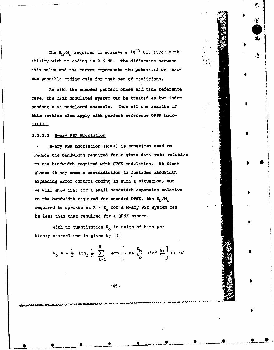
The E/NO required to achieve a 10-5 bit error prob-
ability with no coding is 9.6 dB. The difference between Ithis value and the curves represents the potential or maxi-
mum possible coding gain for that set of conditions.
As with the uncoded perfect phase and time reference
case, the QPSK modulated system can be treated as two inde-
pendent BPSK modulated channels. Thus all the results of
this section also apply with perfect reference QPSK modu-
lation.
3.2.2.2 M-ary PSK Modulation 6
M-ary PSK modulation (04 4) is sometimes used to
reduce the bandwidth required for a. given data rate relative
to the bandwidth required with QP5*K modulation. At first ' •
glance it may seem a contradiction to consider bandwidth
expanding error control coding in such a situation, but
we will show that for a small bandwidth expansion relative
to the bandwidth required for uncoded QPSK, the Eb/No
required to operate at R a R for a M-ary PSK system can0
be less than that required for a QPSK system.I
With no quantization R in units of bits per
binary channel use is given by (41
MR- - l exp mR -- sin2 - (3.24)10o ! E N,
k-l V
"-45-

* °
m®
where - 2 m Since the bandwidth of a PSK system is appro-
ximately equal to one cQver the channel symbol period, the
octal- PSK system only requires 2/3 the bandwidth of a
QPSK system for the same data rate and a 16-ary PSK system
1.only requires I the bandwidth of a QPSK system. Figure
3.12 compares the Eb/No ratios required to operate at R - Ro
versus the bandwidth expansion relative to an uncoded QPSK
system for M -*4, 8, and 16 PSK systems. The larger alphabet
sizo systems are seen to have an Eb/No advantage for small
bandwidth expansions.
Several methods of quantization have been used forthe octal-PSK demodulator outputs. One method is to quan-
tize the in-phase and quadrature outputs so that the signal 0 0space, consisting of signal components every 45 on a circle
of radius /EI, is divided into small squares (see Figure
3.13a). Another method is to divide the received signal space
into pie-shaped wedges depending on the angle of the received
signal component (see Figure 3.13b). The particular quanti-
zation technique will depend on implementation considerations.
The same comparisons ;-resented here for operationat R u R can be performed to compare the minimum possible
Eb/No ratios based on operation at channel capacity.
-46-
.. *.

I' 0x
I Oi4,
II 4:
.,. . ' g I
a0 T 0
-47-
"- I z4j•
U '
P. -4 -47-
• • • o . ...... .•. • Ii .... .... •e

QuadratureComponcnt
I I I - Signal Lccatic""" •s •-- I . • ..
S I In-haseTT 2T 3T -s Component
SQuadrat.ure (a) •
"2"**
SComponent Half Interval
QuaSignalr (a) Si
HafIterval
Signal Locatior
E-s a! reeie sybo energ
""spac 5.625f per in-Sqni zt terval
-4Sigal Locatio,
Iilll///// I"I -Half Itra5**'*/ -// - -5 -- " -- n,.ra
**". " - - ---- - -= In-.!hase"-."'(b) /s Coz..•onent.
"z.'J T- quantization parameter
•:• Es - received symbol energy
4 Figure 3.13 Diagram~s of the first qu~adrant signal-N' space quantization zrnter';als for two possibl,•.'d 6-bit quantization technizues for octal-PSK.
i -4 a-

However, it is usually more difficult to obtain closed form
expressions for C than for R0 . Also for small channel
"symbol energy-to-noise ratios we have (5]
CS
-'o (3.2S)
So the comparisons based on operation at channel capacity
produce approximately the same results as those based
on operation at R - Ro.
3.2.2.3 DBPSK Modulation
As mentioned previously, differentially coherent
phase-shift keying produces a channel with memory. While
some codes have been designed especially for channels with
memory [7-10], the performance of most of the more powerful
coding systems are degraded when they are used on such
channels. To remedy this situation (i.e., to make the
channel appear to be memoryless) simple interleavers
can ne used as illustrated in Figure 3.8. The potential
coding gain of such an interleaved/deinterleaved DBPSK
channel is discussed here. The size of the interleavers
will depend on the type of coding and will be discussed
in later sections.
With no quantization the computational cutoff rate
"for this channel is I5]
R - log 2 11 + PlWe - 0) P(x/e =-l)dx
.a (3.26)
-49-
S
* ... 0 .. . . . •_... _

7-0
where P(x/e - e ) is the probability density functicn ofthe demodulator output random variable given that the phasechange of the transmitted symbol from the last to the present
symbol is 9 For DBPSX the transmitted symbol phasechanges are 0 or r radians. These density functions are"given in Reference 6. Substituting these density functions"in (3.26) yields.
R i~lo 1 ex(-R..)f (R i) (3.27)
. where
.f a) 1 a h dic (3.28)m-O k-0
The Eb/NO ratio required to operate at R - can bedetermined by numeri-ally integrating the integral in
(3.28). Of more interest is this Eb/No value with im- p *plementable quantization techniques.
Figure 3.14 shows this Eb/NO value versus bandwidt-iexpansion for 1- and 3- bit receiver quantization.
i The hard quantization results were obtained using(3.13) with a channel symbol error probability of
•.: 9 " e xpe... 9 (3.29)
3-.[
i..%o.0
-5so-5
'T".,

0 '6a.
\OW 0
* *
14 1
zoII I.
afl' .
4J' I
* I
44003
em UT H/
14 a -
- ~1 M
-SI.-

(3.1)wit N- an ,trasiio
The soft rjuantization results were obtained using '.1(3. 21) with N - 3 and P'" P07" The PJ transition •'
probabilities are the probabilities of being in the dif-
ferent quantization intervals given the transmitted symbol
phase change is zero. These can be determined from the
probability distribution function defined by
P x) - Probability that the demodulator output
random variable is less than or equal to
x given that the transmitted symbol
phase change from the last to the present
symbol is 0
Integrating the density function of (61 gives' this
distribution function 5 0
F b
0- -mR __ 2-R -
1-(x~u . exp, ( E -2x) t
-5 b forx>0' rNo foI
(3.30)
-52-
.%
* 0 0 S _ ~r~,.

,hen the probability of the demodulator output random
variable being in the quantization interval betwen T1 andT2 (TI< T2) is just P (T - .(Tl) The quantization
parameter T was varied to determine the optimum (i.e., the
Eb/No required to operate at R - RO was minimized) value
and in the regions of primary interest T = .7 was best.
As with the coherent PSK case, R0 is relatively insen-
sitive to small changes in this parameter.
Figure 3.14 shows that lower rate (R ) codes
will not necessarily improve the coding performance with
this type of channel. This somewhat unexpected result
can be explained by noting that as the code rate is de- e.
creased the channel symbol energy is decreased and thus
the phase reference becomes noisier. With the coherent
PSX channel a perfect phase reference was assumed. In
practice, the non-ideal phase reference will contribute
a:i Z/No loss which will increase as the code rate is
decreased.
Figure 3.14 again illustrates the gain which
can be achieved with soft quantization of the demodulator
outputs. For a rate 1/2 code hard quantization is 1.3 dB
inferior to 3-bit soft quantization.
5 -3
• • • •.. .. .. . .. .. . • ... ... .. •. .... .. • .. ..- -..- -.... • ...-
Comparing the DBPSK results of Figure 3.14 with thecoherent BPSK results of Figure 3.11 it can be seen t-1' the
potential coding gain of the DBPSK system is significantly
less than that of the BPSK system. Figure 3.15 shows thepotent"al coding gain based on operation at R R - 1/2 S
for BPSK and DBPSK systems.
The minimum possible Eb/No ratio determined basedon R < C can also be obtained for the hard and 3-bit soft Squantization cases using (3.14) and (3.22), respectively.
The results are plotted in Figure 3.16.
3.2.2.4 Ncncoherently Demodulated MFSK
The most common application of this type ofmodulation/demodulation is in anti-jamming frequency-hopped
systems and time-diversity Rayleigh fading channels inwhich one of 22 different, properly spaced, frequencies • Oare used.
With a demodulator consisting of M - 2m square-lawenvelope detectors and no quantization the computational 0
cutoff rate for this modulation/demodulation with additivewhite Gaussian noise can be computed. The result showsthat the "b /N0 ratio required to operate at R - Ro isa monotonically increasing function of the code bandwidth
expansion. So such a channel is not an attractive can-
I
-54- S
e . .. .. • .. .. .• ... . .. . .. o . . . • • • ... ... • . ... •

0-4
InI-.4
0 c
04 i0- .4
41 - 6~'
- .0 v c0 )-d '4v UO "4v ad UO PO WS P T U VV 6UT OZ TVr-u~a40
I I I I I
IOa
KQ C
z MO
1w,.- ~lo\
EP UT t4/ 0

didate for error control coding with additive white Gaussian
'noise.: However, this system is very useful in jamming or
fading environments.
"-To implement such a system the matched filter
outputs would be quantized. If each matched filter output
is quantized to N bits, a total of N2m bits per received
symbol are required. For large m such a system becomes
difficult to implement. However, systems with 8 matched
filter outputs and 2 bits of quantization per filter have
been used effectively in non-Gaussian noise environments
with dual-3 convolutional codes. These results will be
discused in Section 6.
3.2.3 Independent Rayleigh Fading Channel
.As noted in Section 3.1.2, diversity can greatly
improve the performance of communication systems on a
Rayleigh fading chaunel. Coding can reduce the diversity
requirements (i.e., the order of the diversity) and provide
an energy-to-noise ratio coding gain.
The computational cutoff rate for this channel with
noncohererntly demodulated 2m-ary MFSK and no quantization
is [4]
Ro r 2 log1 (3. 31)o 2 1+4 (2 m-1 ) p (l-p)
I5-57- a-•
~ ~ . . . . . . -.----- - - '.
* 0 00 0 00 * .
where O
p- (3.32)
2+mR ,H A
The units of R. are bits per binary channel use and
E;/No is the mean information bit energy-to-noise ratio.
Curves of the i/NO ratio required to operate at
R - Ro versus the bandwidth expansion are givren in Figure
3.17 for binary and octal MFSK. This figure also gives
this 2/No ratio for a hard-quantized binary FSK system. This
ratio was obtained using (3.13) with a channel error pro-
bability given by (3.32). This figure shows that the
difference between the potential performances of soft and
hard quantized coding systems on this channel is even
larger than on the additive white Gaussian noise (AWGN)
channel. On the AWGN channel fo:? a code rate of 1/2 the
energy-to-noise ratio difference was 2 dB while here it
is 4.9 dB.
-58-
* 0 o,_ S 0 .. . 0 . . 0 .. ..... . . .... . .. _

r Jm
a I!•I i.e H ,,•
F_ Ij 17
0••i
L. -, N'q "
o-/ '.-.
M,:
- "fl-e " ...,,..,,..,J ,
• . .. . o .. .. .. .0 . .. .. . • . . . ! . ... • . . .. 0 • .. . . . ... • . O

4.0. Block Codes O
For this class of codes the data is traji5mitted
in blocks o' symbols. For every k encoder input symbols,
n-k parity-check symbols are added to produce a total Sof n symbols to transmit. The code rate is k/n.
The more successful block coding tiaW hiques have cen-
tered about finite-field algebra- concepts.
Linear block codes can be described by a k x n
generator matrix G. If thw A-symbol encoder input is
represented as a k-dimensional column vector, x, and the
encoder output by an n-dimensional column vector, y, the S
encoder input-output relationship is given by
y- xG (4.1)
So the n-symbol encoder output blocks arv linear al-
gebraic combinations of the rows of the generator matrix.
In the binary symbol case, the output blocks are bit-by-
bit modulo-2 sums of the appropriate rows of G.S
Usually block codes are decoded using algebraic
techniques which require the deodullator to make a hard
decision on each received symbol. In 3ection 3 it was
shown that such hard quantization unnecessarily reduces
the potential performance of the coding system. For the
additive white Gaussian noise channel with BPSK or QPSK
modulation the potential coding gain of a finely quantized
-60-
*SO O • • • Ct tb¶%9~ %.' • • td ,r- • •

S
7 0
coding system is about 2 more than that of hard quan-
tized system. Recently several soft decision coding
"techniques have been proposed for block codes (11,12]
which, at least for some particular codes, seem to recover
most of this 2 dB loss. However, the implementation corm-
plexity of such systems is usually much greater than
that of Lie corresponding hard quantized system. In D
"general, when soft decisions are available a convolutional
coding technique which easily adapts to soft decisions is
preferable.
Another disadvantage of block codes as compared to
convolutional cods.z is that with block codes the receiver
must resolve an n-way ambiguity to determine the start of * .a block whereas with Viterbi-or feedback-decoded con-
volutional codes a much smaller ambiguity needs to be
resolved (see Section S.i.12).ipIn spite of these disadvantages, block codes are
sometimes useful on channels where only hard decisions
S are available and the data is presented in blocked format.
Another ccmmon application of Ylock codes is 0
for error detect.on. That is, instead o' crying to correct
3 errors the decoder performs the simpler task of just da-.
tecting if one or more errors have occurred in the block.
AL 1 -61-
* ,CJJIii )M A T.1M AC .~.f' l C*~l~ .~ .C
.JI

*O0
Such erroi detection systems have been used in appli-
catinis where a feedback channel is available to tell
the transmitter to retransmit the blocks where errors
have been detected.
The selection and estimated performance of
blo.,k codes are usually based on the block distance
properties of the code. The distance (sometimes called
Ramming distance) between two code words or sequences
with an equal number of symkols is defined as the number
of positicnu in which the symbols differ. The minimum
"distance of the code is defined as the minimum distance
between any two different encoder output words (or se-
quences or blocks). Also the performance and distarnce
properties of linear block codes are independent of the • 0encoder input sequence, so for analysis purpose without
loss of generality the all zero sequence is usually as-
sumed to have been transmitted.
For a fixed code rate and block length the goal
is to choose a code with a large minimum distance. Then
the dacoeer can more reliably detect or correct channel
errors in the received block. A block code with a minimum
distance of dmi is capable of correcting any combination
of (dmin-l)/2 or fewer channel errors or detecting
any combination of d-l or fewer channel errors, where
.'A
-62-
A.A..

[x]I is the integer part of x. However, while the .mini- 4
"mum distance of the code may' be sufficient to gua.;vntee
the detection or correction of a certain number of errors,
the particular decoding algorithm may not be capable
of such operation.
The performance of block codes with hard receiver
quantization is usually determined by assuming that the
~ ' decoder can correct any combinination of E, E < (d-l)/2
'. or fewer channel errors and no combination of more than
E errors. Such a decoder is called a *bounded distance
decoder 3 . Then on a binary symmetric channel the bloch
*':" error probability, Pblock' is the probability that more
than E errors occured. Since there are ()differentways of having i errors in n symbols, the block error
probability is
P M (n p i i(1..P) ni (4.2)block E )
i-E+l
WN' The bit error probability dcpends on the particular
code and decoder. Usually block codes are selected to
have given block weight properties and codes are called
equivalent if they hawe the same set of block distances
"(or weigkbts, i.e., number of nonzero encoded block
".V symbols when the all zero input is assumed). However,
the bit error probabilities of these so-called equivalent
"-.• codes may vary. To determine this error probability,
-.?
i -63-
- S AIj.oJt"~2 &..A As ~ ~~ ~. b~.b % . .. ,~.~ ..

assume that the decoder can correct up to E channel errors.
These errors are then corrected in the received sequence.
The final step is to determine the encoder input block
corresponding to the corrected received sequence. This
step can be simplified by using a systematic code. Such
a code has the property that all the k information symbols
are sent unchanged along with n-k parity symbols. In
general, every output could depend on every input. It
"has been shown (5] that for every linear block code there
exists a linear systematic block code with the same distance
. properties. Therefore, systematic block codes are commonly
used. We wiLl assume systematic block codes in the
remainder of this report.
PThe bit error probability for this type of decoder I 0
, with a systematic code can be estimated by assuming that
the error rate of the corrected received sequence is equal
.b to the error rate of the encoder input information symbol
sequence. Then the bit error probability can be expressed
as
°'b n
"" b n (1-BeP )l'l' (4.3)
"i-E+l
S where a is the average number of symbol errors remaining
in the corrected received sequence given that the channel
L
j -64-re '
1... .. •••, . . .

caused i symbol errors. Of course, 6 0 for i < E.
When i > E, Si can be bounded by noting that when more
than E errors occur a decoder which can correct at most
E errors would at best correct E of the errors and at
worst add E errors. So
Si -E< Ai ! i + E ,i > E (4.4)
The decoder performance can be slightly improved by
passing the received sequence unchanged when the corrected
*. received sequence is not a valid code word. In either case
for the majority of codes for which B0 has not been
determined, B£ - i is a good approximation.
When a block code is used for error detection only,
the decoder fails to detect an error in the block only when
the error sequence transforms the encoded sequence into
another valid encoded sequence. By the linearity of the
code this implies that the error sequence is equal to a
valid code word. This probability of an undetected error
can be expressed as
np- Ai Pi(1-P)n-i (4.5)
i-E÷1
where Ai is the number of encoded words of weight i (i.e., D
the number of encoded words with i nonzero symbols). Some-
times it is also of inteý.ast to determine the probability
II
-65-
-- -- -- --

J O
of r•ot detecting an error under any channel conditions. On I.a binary symmetric channel the worst channel is when the
channel error probability is 1/2. Substituting p- 1/2 in
(4.5) and using the fact that there are 2k- 1 codewords of
weight E+l to n and one codeword of weight zero gives 9
P / (2 k _ 1 )2-n < 2 - (n-k)
This bound is sometimes used as an upper bound on the
undetected error probability for any channel error rate.
While this is valid for Hamming codes, it is not true in
general (131. Nevertheless, the P 2 -(n-k) bound gives
a first approximation to tiis worst case undetected error
probability.
When the information and encoded symbols of a
block code are from some nonbinary alphabet and the pro- •
bability of any channel input symbol being changed to any
other symbol is the same for any nonidentical input-output
symbol combination and p is taken to be the channel symbol
error probability, then (4.2) and (4.5) still apply and the
bit error probability of (4.3) becomes the symbol error
probability.I
The block code error probability formulas presented
thus far have been for hard receiver quantization. Decoders
capable of using soft quantized input, are possible, but
they are more difficult to implement. The simplest type
I-66-

1 10
of soft quantization is one in which three, rather than two,
quantization intervals are used. This additional interval
could be used to erase unreliable symbols. Forney [161
shows how the hard quantization block decoding technique-s
can ba extended to take advantage of such a recei,rer quiui-
tization scheme. This type oZ decoding is sometimes called
erasure-and-errors decoding. S
If the decoder doe•s erasure-and-errors dacoding,
the code minimum distance is d, and the maximum numver of
errors that the decoder can correct is E, then a decoded s
error occurs when the number of errors t and the number of
erasures s satisfy 2t+s > d or t > E+l. So if the pro-
bability of an erasure is p x and the probability of a
channel error is PE' then the block e..-or probability is
[161
P 2 nt (St t •x (-e"PE'Pz -PblockE Z, PE
t-0 s-d-2t
where
n• ltt(n-s-t)!
In ths following subsections the structure and
performance of several specific block codes are examined.
-67-
S
* 9 -.. 9

4.1. Hamming_ Codes
Hamming codes are the simplest nontrival class
of codes with n - 2*-i (m - 2,3, ... ) encoder output
symbols for each block of .k - n-m input symbols. These
codes have a minimum distance of 3 and thus are capable
of correcting all single errors or detecting all com-
binations of 2 or feaer errors. Although Hamming codes
are not very powerful they belong to a very limited
class of block codes called perfect cod-s. An e-error-
correcting, e - t(d-l)/21], code is called a perfect code
if every n-symbol sequence is at a distance of at mst
e from some n-symbol encoder output sequence.
Hawing codes are usually described in terms of
an n x (n-k) dimensional parity check matzix 151, H, 0 0
with the property that for each n-dimensional encoded
output word y
I
X a - o_ (4.7)
For Hamming codes the n rows of the parity check matrix
are equal to all positive nonzero m-bit sequences. Given
ai parity check matrix, a generator matrix can be determined(5].
If the binary additive noise sequence is represonted
by an n-dimensional vector z, then the received signal is
.x G_ z (4.8)
-68-
II
* * 0 S

where 0 denotes bit-by-bit modulo-2 addition. -,
Decoding is accomplished by multiplying this binary
vector by the parity chack matrix to form an n-k - m di- 0
mensional syndrome vector S. Using (4.7) we have
S_ G H 0 z H_ H (4.9)
Because of the form of l, this m-bit syndrome specifies
the locations of Any single error which can then be cor-
rected. If the syndrome is zero, the decoder assumes
no errors occurred. P
The weight distribution of Hamming codes have been
determined. Expressed as a polynomial this distribution
for the binary case is (141
'40
A(zl) ~ A~ 3Zi-0
-~ +i~ no 1+ I 4.10)
where Ai is the number of code words of weight i. This
weight enumerator polynomial makes the computation of the
undetected error probability possible. 0
From (4.2), (4.3) and (4.i) the block, bit, and
undetected error probabilities are
-69-
b4 ... ,)• , "•.,'•sd",'• .', ,: ,.'•:,:.•-.;• -:',•, • •:'•" "1.• .;• • ,'-'•€-'• • '• r-'•- • , -€z--'.'•"•( : ''•'u •'•- " r. :s ,.,•-.•r.,•, .'"

nI
P 4 (n) iblock j _i) n-i
"- p - p(1-p)n-l (4.12)
and
-D
1-(ip)n [A(-P1 ) 1 (4.13)
where (4.12) uses the 8 ± 1 approximation for i > 1. 0
Figures 4.1, 4.2, and 4.3 show thess probabilities
versus the channel error rate for a - 3, 4, azd 5. The
channel error rates can be determined from Sec-.:ion 3.1
for the binary zemoryless channel case. With interleaving
the bit error probability versus lb/No results for fading
channels or for differentially coherent or nonbinary modu-I
lation can also be used. Just £nterprst the bit error
probability versus Fb/No results of Section 3.1 as the chan-
nel error rate versus the channel symbol energy-to-noise 'ratio,
7
-70-
.. .a _ S .. . .• ....

10 O1l0.~1 .... ,"
10":3,3
n-4 *
II
-31t
10s
W 10
- 6
"Channel Error Probability p
Figure 4.1 Block error probability versuschannel error probability forblock length n-2m-1 Hammingacodes with m-3, 4, and 5.
-71-

1 O10-2
b
x-3
-4-
~R,
10
. -
>,10-4"A ~1o I
o 10"
I~4 4
1 10 10- 100
Channel Error Probability -p
Figure 4.2 Bit error probability versuas channelerror probability for block length
-4-
n 2 -i Hamming codes with m -3,4,and S.
-72-
10P

10-2%S
10-3
0S
$ 10-4 .vm
4105
0
0
10
0-7
'
101 102 10-31-
Channel Ercor Probability *p
Figure 4.3 Probability of an undetected error versuschannel e~rror probability for block length
na 2 M-1 Hammning codes with mm3, 4, nd .5.
-73-
,W 1 %

E/ 3 . To obtain the coded system information bit energy-
to-noise ratio use
~~- rE I Es (4.14)"'
0 0
For Hamming codes (4.14) becomer'
Eb 2m- Es (4.15)
0 223 -l-m N0
With these changes the probabilities of Figures 4.1, 4.2, and
4.3 can be plotted versus Eb/No. The bit error probability
result for an additive white Gaussian noise channel is
given in Figure 4.4. The coding gain can be determined
as the reduction in the Eb/No required to achieve a spec-
ified error probability with the coded system as compared
to the uncoded system.
Table 4.1 summarizes che Eb/NO ratios required to
achieve a 10-5 bit error probability with Hamming coding
for several modulation/demodulation tachniques with ad-
ditive white Gaussian noise (AWGN) and Rayleigh fading.
4.2 Extended Golay Code P
One of the more useful block codes is the binary
n - 24, k - 12, i.e, (24,12) extended Golay code formed
by adding an overall parity bit to the perfect (23,12)
Golay code. This parity bit increases the minimum distance
-74-
/
* • .. . . . * .. •: . . . . . . • .... . A.... . • _ • . O

0*
1-2 O
S10-3
loo
Uncoded ,
. 10-4 3
0 105 J
F j Saal,,
10 ~
10-70
4a 5 6* 0 1
b"-l' l i
m - ,t 4 l ng 5n an ".GI chane. i
-75-
.. . : •
0 0*.
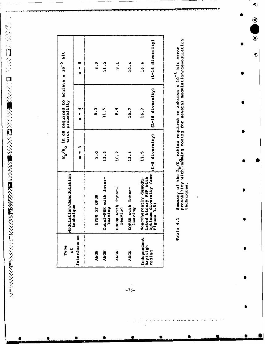
$4 " 4
.IJ 0 S144
040
.0 A
-440, >9 w C~
0 >a 41
Q 4 l0
$4 C6
c~ 144 Va4-.4 0a41
3.0 11 a>1 0-4a
bp%14A 1.40Zk74a -4 ý0-4 c
a,4 -. A C
A1 A . %
0 co 01ac4. ..0 "0 Q@4 31 31 Uý
. . .-4 4 1a0 V04 a~ 4 0 U) 4 Q W 0 J 0
a- 4 4 as-4 as4 c4 Sj *a
C6 604 W .
"4 ~C :9 0441 Vc m 6 6c oc >
C 0
-76- 44u

of the code from 7 to 8 and produces a rate 1/2 code
"which is easier to work with than the rate 12/23 of the
(23,12) code.
k Extended Golay codes are considerably more
powcrful than the Hamming codes of the previous section.
The price for the improved performance is a more complex
decoder and a lower zate, and hence a larger bandwidth
expansion. Decoding algorithm which make use of soft
decision demodulator outputs have also been proposed
for these codes (11,12). When such soft decision decoding
* algorithms are used the performance of the extended Golay
code is similar to that of a simple Viterbi-decoded con-
p volutional coding system of constraint length about 5 (see
Section 5.1.10). While it is difficult to compare the im-
plementation complexity of two different coding systems, it
can be concluded that when only hard decision demodulator
outputs are available, extended Golay coding systems are
of the same approximate complexity as similar performance
convolutional coding systems. However, when soft decisions
are available convolutional coding is superior.
The hard-decision block and bit error probability
expressions of Section 4.0 assumed that the decoder was
capable of correcting any combination of E or fewer errors
and no combination of more than E errors. With perfect
codes, such as the Hamming codes, with E - [(d-l)/'21]
-77-
I
• • • , , , e . •e,, , ,L•.-- * S

A
this is always the case. However, with an extended lolay I1 code the decoder could be designed to correct some but
"not all 4-error patterns. Usually, in order to simplifythe decoder implementation the decoder is imp:emented
0in such a way that these 4-error patterns cannert be cor-rocted. Since for extended Golay codes only 19% of týe4-error patterns car. be corrected we will assume the
decoder cannot correct these 4-error patterns. Then theblock, bit, and undetected error probabilities for hard-"decision decoding can be determined from (4.2), (4.3) and
S(4.5). The results are 0
24
P E a4 (24). pi/_PZ4 -i24J "P~lP (4.17)
"" Pu " ( - 4 pand
u) (4.18)
where the B0 coefficients and the coefficients of theweight enumerator polynomial, A, are given in Table 4.2.
"Figure 4.5 gives tJese probabilities versus thechannel error rate. As in the previous section the channel
-78-

0
A- Number of Code Words of
0 0
1-3 0 0
4 0 4S
50
6 120/19
7 0 8
8 759 8
9 0 2637/323
10 0 3256/323
11 0 3656/323 1s
.1
12 2576 12
13 0 4096/323
14 0 4496/323
15 0 5115/323
i5 759 16
17 a 16
18 0 336/19
19 0 16
20 0 20 .
21-23 0 24
24 1 24
Table 4.2 Weight enumerator and B. coefficientsfor the extended Golay 6ode (12).
-79-
.
0 0 S 00 90
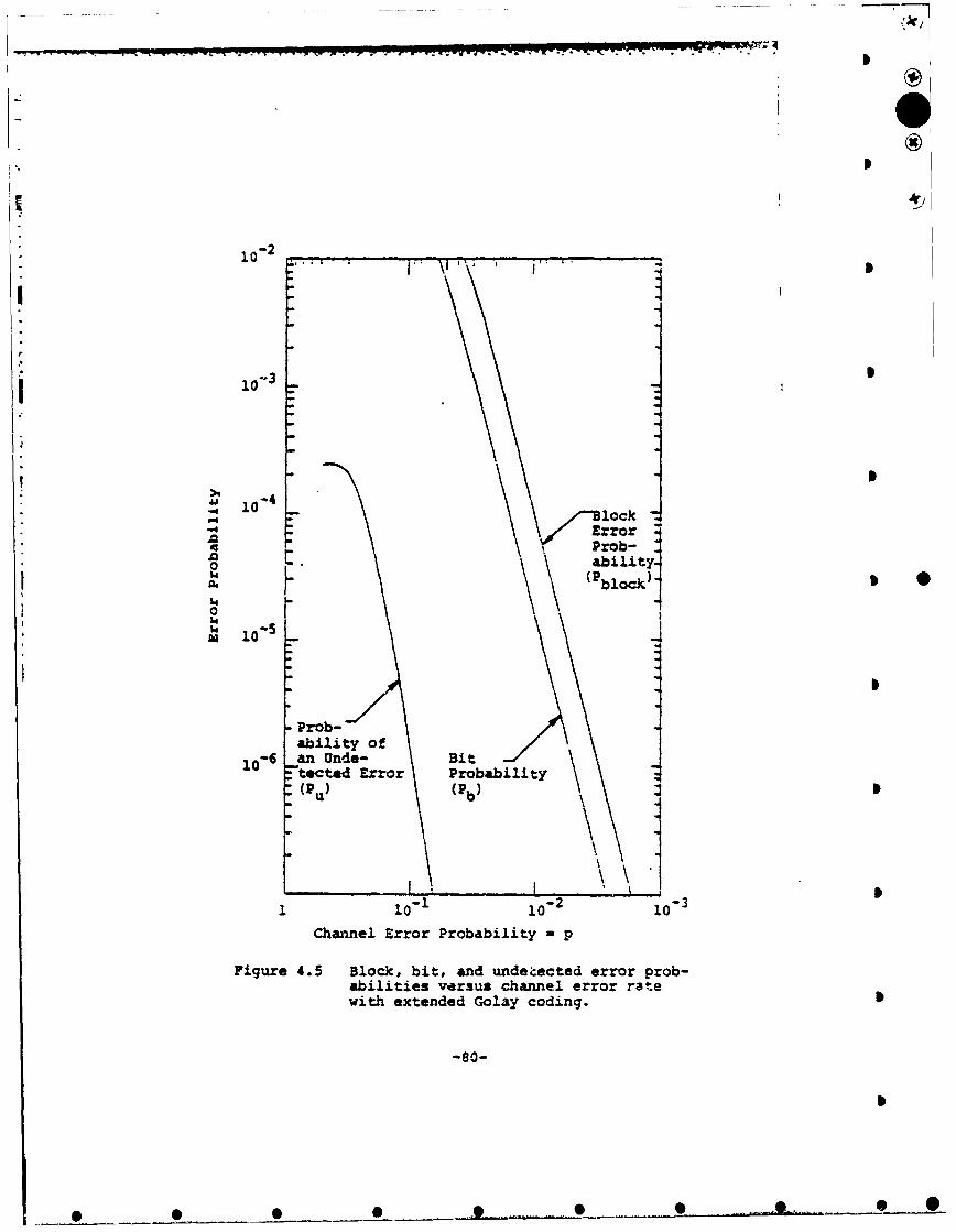
I 'r
010
Lp
S10~ Rlc4- 4
"4 1014 Error
.0 Prob-L.- I' ability-S" (P~block)I
0a.
24 10"
Prob-ability of
16an Cnde- Bittected Error Probability(P U) (Pb) D
L i10-I 10_2 10- 3
Channel Error Probability - p
Figure 4.5 Block, bit, and undeCected error prob-abilities versus channel error ratewith extended Golay coding.
-80-
S.... • ... . . .. .... .• ... ... • . ... .. •.-... • . • • .. .... . • . .. ....... • -. _ •-dp

* (g
.1
error rate can be determined from the results of Section
3.1. Using these results the hard-decision coding perfor-
mance for coherently demodulated BPSK or QPSK on an AWGN
channel are given in Figure 4.6. Figu:e 4.6 also shows the
bit error probability obtained with a soft-decision decoding
algorithm proposed in (111. The soft-decision algorithm jis seen to recover most of the 2 dB hard quantization loss
* determined in Section 3.2.2.
Table 4.3 gives the Eb/NO ratios required to obtain
a 10- bit error rate with the extended Golay coding and Nseveral alfferent .odulation/demodulation techniques for
AWGN and Rayleigh fading channels.
4.3 BCH Codes
Bose-Chaudhuri-Hocquenghem (BCH) codes are a powerful
class of codes which havy well defined decoding algorithms.
A large selection of block lengths, code rates, alphabet
sizes, and code minimum distances are possible. The most
common codes use a binary alphabet, an encoder output
block length of n - 2m-1 (m a positive integer), and, of
course, the largest possible code minimum distance.
A detailed description of BCH codes requires ela- Nborate algebraic developments and is beyond the scope of
this report. The main point is that while a description
of these codes and their decodirg algoritnms is somewhat
-81-1
0 S S 0 I

2I
102
10- , .1o 2
iy
10 Sof Rceive H4ard Receiv
Quatiztio ,:O' eRceve uanazaLot IzC
(12 ti
o 10
WIBoit Errrrr
ProbaPobbil dUindetected Erto (PHorrd Recitv
10- Sot Recverive Quant ion o ioQAun ihatinne
1--7i
vesu Eo5 ~ b~ IN o0o Ko Kmdltoa
-82
ONOW

a 0
444
0 41
41.
00 049 0. 0
P4 a
-.4 '
.0 0 0 0C 40
-4 Z= 0'
a 4 4 -4 tr 41.0 %
1. - % ,~
44 0- a 0 0
V v A
0 0 0 -A 3t0
0 '0 C4 0 c~ 0 U,
V0- C c 14
a 0 CL >910
>1lZ 0 Vm ( t toc oc A PC 14.
P-40
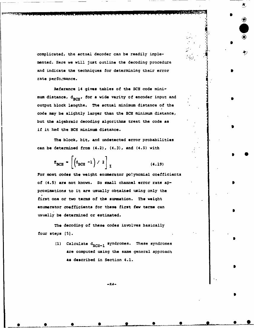
""4 .
'"4
.. .
complicated, the actual decoder can be readily imple- .:' "
mented. Here we will just outline the decoding procedure
and indicate the techniques for determining their error S
rate perfo.-mance.
Reference 14 gives tables of the BCH code mini-
mum distance, dcs, for a wide varity of encoder input and
output block lengths. The actual minimum distance of the
code may be slightly larger than the BCH minimum distance,
but the algebraic decoding algorithms treat the code as
if it had the BCH minimum distance.
The block, bit, and undetected error probabilities
can be determined from (4.2), (4.3), and (4.5) with
E . [(d.CH 1i 2j (4.19)
For most codes the weight enumerator po!ynomial coefficients
of (4.5) are not known. So small channel error rate ap- S
proximations to it are usually obtained using only the
first one or two terms of the suunation. The weight
enumerator coefficients for these first few terms can Iusually be determined or estimated.
The decoding of these codes involves basically
four steps (5].I
(1) Calculate dBCH-1 syndromes. These syndromes
are computed using the same general approach
as described in Section 4.1.
-AA-
I
* _ O __ ,_ •O _, __

(2) Find the coefficients for an e-degree error
locator polynomial where e, < E~ is
the number of channel errors. The technique
for doing this is referred to as the Berlekamp
Algorithm. This polynomial has the significance
that its roots give the locations of the channel
errors in the received block of symbols.
(3) Find the roots, and thus the locations of the
errors, of the error locator polynomial. The
usual technLque for doing this is referred
to as the Chien Search (5].
It involves checking each of the a code symbol
locations to see if that location corresponds • 0to a root of the error locator polynomial. -.
(4) Find the values of the errors. With binary
codes the errors can be corrected by comple- -
menting the present symbol. With nonbinary
symbols a simple formula is available [5].
This algebraic decoding procedure uses hard quantized
demodulator outputs and thus gives up some potential coding
gain on channels where soft decisions are available. While
extension to soft decision is possible, with the same tech-
niques used for Golay codes, the complexity increases sub- '
stantially..8..
S.5
• °S.2 .
o°-

Figure 4.7 illustrates the bit error probability
versus channel bit error rate performances that can be
achieved trith block length n1 127 codes capable of cor-
recting 5, 10, and 15 channel errors. The results were
obtained using (4.3) with - i. The largest possible
number of information bits per block for the 5, 10, and
15 error-correcting BCH codes of Figure 4.7 are k - 92,
64, and 36, respectively (411.
One special type of BCH code worthy of further
note is the class of Reed-Solomon codes discussed in the
next section.
4.4. Reed-Solomon Codes
Reed-Solomon Codes are a particularly interesting
and useful class of nonbinary BCH codes which achieve the
largest pos:sible codet minimum distance for any linear code
with the same encoder input and output block lengths. For
nonbinary codes the distance between two code words is
defined as the number of nonbinary symbols in which the
sequences differ. For Reed-Solomon codes the code minimum
distance is given by (5)
d = n+l-k (4.20)
An E-error-correcting Reed-Solomon code with an alphabet
of 2m symbols has
n - 2 m-i (4.21)
All
••

II
1*'06
•'LI . ,o2
10"3
41 t- I>, 10. .--3 "
10-. 4\~.~k921
Ii.o k -64
S- k 361
414
S~L
,10 6
10 0- 10
-7- ~Channel Error Rate
• ,! Figure 4.7 Bit error probability versus chan•nel? error rate performance of several-. " block lex~qth 127, BCE codes.
t -87-

and
k 2m-l-2E (4.22)
These codes are particularly good as outer codes
in concatenated coding systems (see Section 7.0). In such
a system the inner code provides some error control by
operating on soft-decision demodulator outputs and then
presents hard-decision data to the outer decoder which
"reduces the error rate to the desired level. Binary inner
code symbols are grouped to form the 2m-ary Reed-Solomon
code symbols. These codes are also sometimes used on jamming
or Wding channels with nonroherent demodulation and 2m -
orthogonal-signal modulation.
The performance of a system with this type of coding
on a memoryless channel can be specified in terms of the *channel symbol error probability ps. If the channel is not
memoryless, it is usually best to provide some interleaving
to break up any bursts. In general, the performance of a
coding system not specificially designed for channels with
"memory is degraded by channel memory. Even channels spec-
-' ifically designed for a channel with memory will be degraded"•-•" if the memory is different than expected. Usually since
the characteristics of channels with memory are difficult
.. to measure, interleaving is a wise approach. Only a rough
•. .idea of the channel memory length and any periodic proper-
"ties of the channel are required to build the interleaver.
3%
iL* IL
* 00.

0*"Also a system with interleaving is very effective with
random errors.
A code which achieven the minimum distace of (4.20)
is called a maximum distance spearable code (151 and the
weight enumerator polynomial coefficients for these codes
"have been determined [161.. The result is21•, k-22-1
-(2m kk-) (2m - 1)1 (limk i ..2E
"for k - 2E+1 (4.23)
of courseA -1 and A - 0 for I < k < E.
"From (4.2), (4.3) and (4.5) the block, symbol,
and undetected a@ror pxzbabilitieu areS2k-i -.1 1 m..±
' Pblock " (z P.'p (4.24)
[•1 -E+1P~ (2*-)i Ps P --
-2-l1 i-E+l
(4425)
and 2 M-1
P A -P 2m-l-iiu " Ai P (4.26)
w e ( )uE+l a
j where (4.25) uses the Bi - i approximation for i ) E.
"4-
I.
P•I
0 099
The bit error probability can be upper bounded
"by the symbol error probability or for specific channels
expressions relating the two probabilities can be obtained.
"For 2m- orthogonal-signal modulation, the relationmhip is
.-'. [1]
P 2 P (4.27) 9.. b• 2M_ sym
Figure 4.8 shows the bit error probability versus
channel symbol error probability obtained using (4.25)
and (4.27) for a n - 31 code capable of correcting various
numbers of channel errors. Figure 4.9 shows the bit error
probability performances of the same codes versus E/No for
.'..* a system with 32-ary MFSK modulation and noncoherent demo- p•--•.O dulation. Results on the performance of concatenated coding
systems which use a Reed-Solomon outer code are given in
Section 7.0.
.9.,
I n
0D

•'2%
100
10-3
44-° 0-
-A
E .1
. -
105
E
E a10"6 7
NN tE '
"101 10-2 10 IChannel Symbol Error Probability - p
Figure 4.8 Bit error probability versus channelsymbol error probability for 32-crthogonal-signal modulation and n-31, E-error-cor-rocting Reed-Solomon coding.
-91-
%i S 0-0g0-

JAN 02 '96 11:19AM TITAN LINKABIT P.3/4
I®
E 4ic EI
m \ I
° o -4,\710 E 2
10-4
-\i I,i0-5
o10 -6
3.5 4.0 4.5 5.0 5.5 6.0 6.5 7.0
Eb/IN° in dBFigure 4.9 P~it error probability versus Eb/INO0 perform-
ance of several n= 31, E-er-or-correctingReed-Solcmon coding systems with 32-aryMFSK modulation on an AWGN channel.
-92- p
• • • 1. _m .... • • , . .. 1 .... • , ,• •

JAN 02 '96 11:20ANI TITAN LINKABIT P.4/4
I 0*
m 5.0. Binary Convolutional Codes
p A rate b/v, constraint length K, binary convolutional
encoder is a b-input v-output linear finite-state device
which can be implemented with K binary register stages and
linear logic as shown in Fiqure 5.1. Each set of v Outputs
depends on K variables of which b are the current inputs and
K-b are state variables. So there are 2K-b different states.
N The constraint length K is defined as the total number of
binary register stages in the encoder. Sometimes the con-
straint length is also defined as the number of state vari-
n able v where
V = K-b (5.1)
Here the first constraint length K definition will be
used.
To make some of the convolutional coding concepts
easier to understand we will describe some of their pro-
perties for the rate R=1/2 constraint length K=3 encoder of
Figure 5.2 and then extend the results to the more general
encoder of Figure 5.1. Figure 5.2 indicates the outputs
for a particular binary input sequence assuming the state
(i.e., the previous two data bits into the shift register)
were zero. Modulo-2 addition (i.e., 0 * 0 = 0, 0 * 1 = 1,
m 1 * 0 = 1, 10 1 = 0) is used. with the input and output
sequences defined from right-to-left the first three input bits
0, 1, and i, generate the code outputs 00, 11, and 01, res-
pectively.
mUm -93- S
S 0 _ .. . 0 9 0 0 _b 0

•J
®Kl-stac. • fe•!s•er 0.: I : i J
:I [ t... €
"..
K 2-stage . "-." "e lS•e. 4 i i I J"" h L•ne •r
:•.:-• < ! '- , Ou•uts 0• i, oc•.€ •
"°t •
:-: °
4
• , i i , i
2- - 1•"
.%' •i .e.
m_
": D2' Constraint Length : K - KI * K2 +...+Kbt
.i
,%
%
,• Figure 5.1 Rate b/v, constraint length K,• convolutional encoder.
|
-94-
S......................... .t ....... ...... ............... ._t .....

p 010001 ...
*~Modu1o-2 addi-tion
p 301O10O1001o*- IV\
C o9- Data SeouaenciSSeq3eflce
Register-
<-ozl- ad,-it-*on
011100"-
Figure 51.2 Rate 1/2 constraint lengthl 3 convolutionalencoder.
-95-

a-x
The outputs are shown demultip3.exed into a single code
sequence. Of course, the code sequence has twice the bit 71
rate as the data sequence. We shall pursue this example
to develop various representations of convolutional codes
and the~r properties. The techniques thus developed will
ithen be shown to generalize directly to any convolutional
code.
it is taditional and instruictive to exhibit a
convolutional code by means of a tret di&gram as shown in
Figure 5.3.
If the first input bit is a zero,tho code symbols
a--* those shown on the first upper branch, while if it is
a one, the output code symbols are those shown on the first
lower branch. Similarly, if the second input bit is a zero,
we trace the tree diagram to the nxt upper branch, while
if it is a one, we trace the diagram downward. In this manner
all thirty-two possibles outputs for the first five inputs
may be traced.
From the diagram it also becomes clear that after
the first three branches the structure becomes repetitive.
"In fact, we readily recsgnize that beyond the third branch
the code symbols on branches emanating from the two nodes
labelled an are identical, and similarly for all the
similarly labeled pairs of nodei The reason for this is
obvious from examination of the encoder. As the fiurth
input bit enters the coder at the right, the first data bitlablld a"ar ienicl, ndsiilrl fr llth
siial*aeldpiso od*Terao for _hi 0is-*

00.00 1
10
O010
01 01010•
I oo I
10 cC O - N
101
00I O1 d Ol
Of$111 a
10 01
10 1
ol0 1
.10
i0 d O! i00
Figure 5.3 Tree code representation for coder ofFigure 5.2.
-97- I
I
S.. . .. 0 1 0 ,
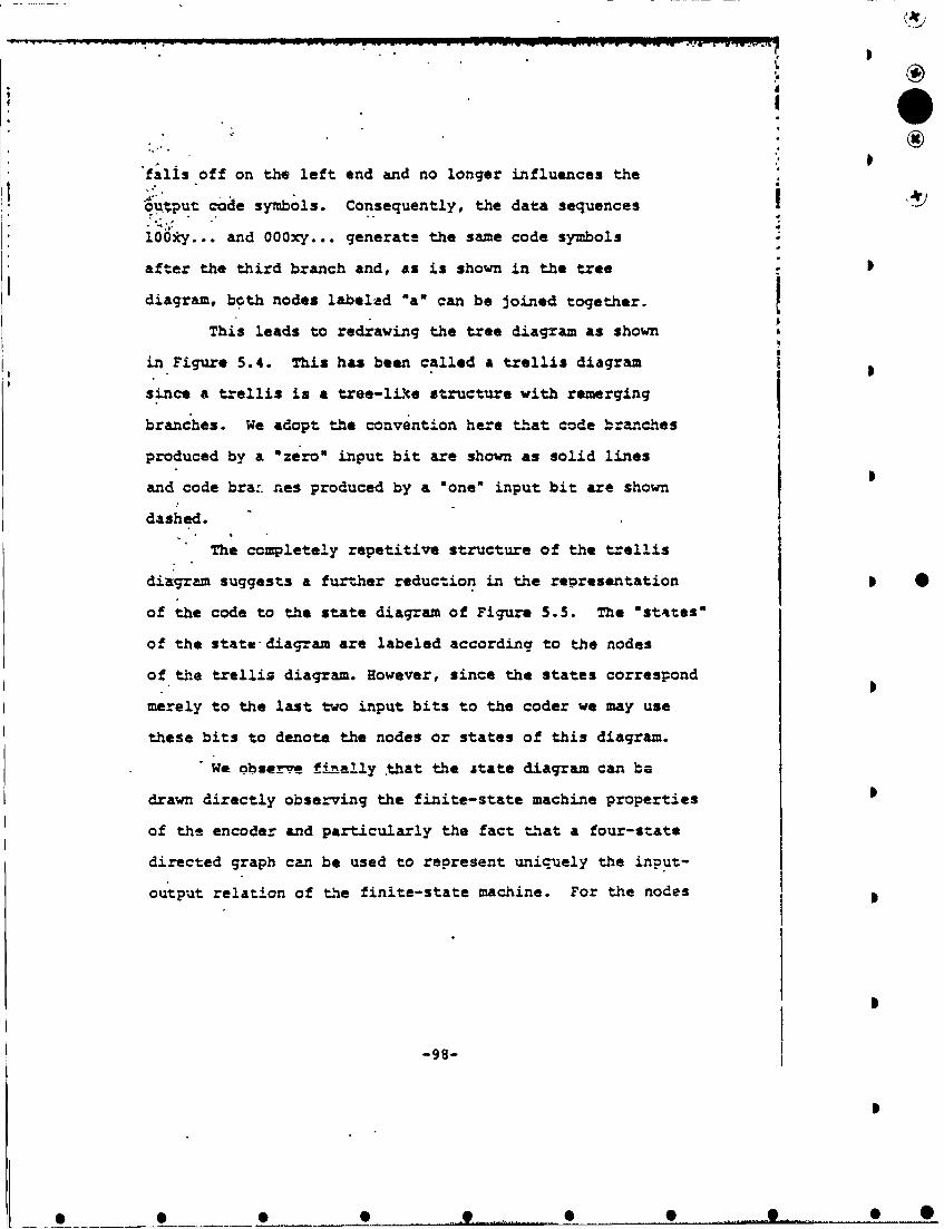
6
falis off on the left end and no longer influences the
Oustput code symbols. Consequently, the data sequences
106xy... and 000xy... generate the same code symbols4
after the third branch and, as is shown in the tree
diagram, both nodes labeltd *a" can be joined together.
This leads to redrawing the tree diagram as shown a
in Figure 5.4. This has been called a trellis diagramI
since a trellis is a tree-i~ke structure with remerging
branches. We adopt the convention here that code branches
produced by a "zero" input bit are shown as solid lines
and code bra.. nes produced by a "one" input bit are shown
dashed.
The completely repetitive structure of the trellis
diagram suggests a further reduction in the representation I0
of the code to the state diagram of Figure 5.5. The "states"
of the state diagram are labeled according to the nodes
of the trellis diagram. However, since the states correspond
merely to the last two input bits to the coder we may use
these bits to denote the nodes or states of this diagram.
We ob_.'rve finally that the 5tate diagram can be
drawn directly observing the finite-state machine properties 0
of the encoder and particularly the fact that a four-state
directed graph can be used to represent uniquely the input-
output relation of the finite-state machine. For the nodes
-98-
I

T iIe
ý 0 h
®
Tin 'AJ
10110 1 2 30
o'o\
I0.0o IO
Figure 5.4 Trellis code representation for coderof Figure 5.2
9.
-99-';hI
K'
O • • eO 0 . ....... •l •
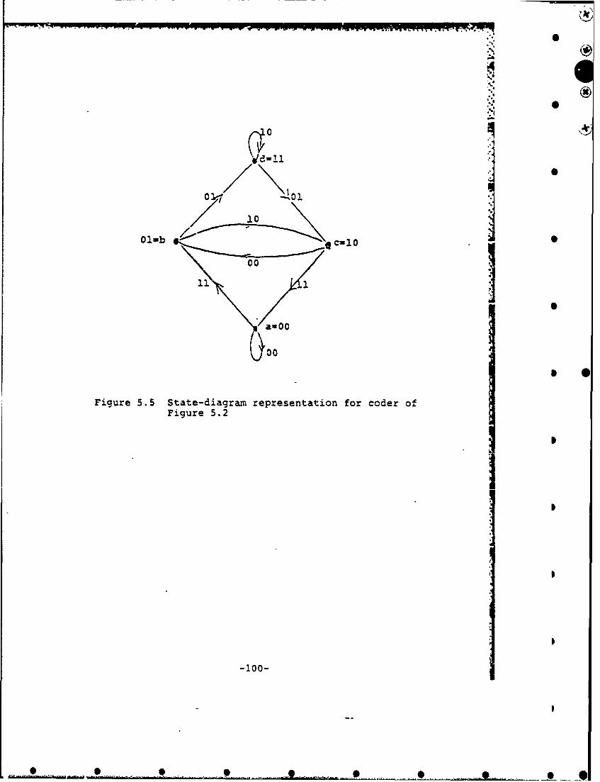
00
1000
011 1o~
a--0
01-b -*cu10
00
0400
Figure 5.5 State-diagram representation for coder ofFigure 5.2
-100-
S, • ,- .. •
0*I
represent the previous two bits while the present bit
is indicated by the transitioa branch; for example, if
the encoder (machine) contains 011, this is represented
in the diagram by the transition from state b-01 to
state d-11 and the corresponding branch indicates the code
symbol outputs 01.
In the following sections we will use these
representations to describe the three main types of deco-
ders for convolutional codes: Viterbi, sequential and
feedback.
5.1 Viterbi Decoded Convolutional Codes
The Viterbi decoding algorithm (20] is a path
maxim,'=-likelihood decoding algorithm which takes advantage
of the remerging path structure (see Figure 5.4) of con-
volutional codes. By pati- maximum-likelihood decoding
algorithm, we mean that of all the possible paths tnrough
the trellis, a Viterbi decoder chooses the path, or one
of the pAths, most likely in the probabilistic senso to have
been transmitted. To simplify the Viterbi decoder descrip-
tion we will describe it first for a hard quantized channel
and then generalize the description to a soft-quantizeO
channel.
5.1.1 The Viterbi Decoding Algorithm for the Binary Sym-
metric Channel
On a binary symmetric channel, errors which trans-
-101-
S S 0 0 * L •.. .. ...

I I P.
form a channel code symbol 0 to 1 or I to 0 are assumed
to occur independently from symbol to symb..! with prob-
ability p. If all input (message) sequences are equally
likely, the decoder which minimizes the overall path N'
error probability for any code, block or convolutional,
is one which examines the error-corrupted received sequence
yj y2 .... yj ... and chooses the data sequence corresponding
to the transmitted code sequence x1 x2 .... x j... which is
closest to the received sequence in the sense of Namming
distance; that is the transmitted sequence which differs
from the received sequence in the minimum number of symbols.
Referring first to the tree diagram, this implies
that we should choose that path in the tree whose code se-
quence differs in the minimum number of symbols from the
received sequence. However, recognizing that the transmitted
code branches remerge continually, we may equally limit our
choice to the possible paths in the trellis diagram of Figure
5.4. Examination of this diagram indicates that it is un.-
necessary to consider the entire received sequence (which
conceivably could be thousands or millions of symbols in
length) at one time in deciding upon the most likely (mini-
mum distance) transmitted sequence. In particular, immediately
after the third branch we may determine which of the two-
paths leading to node or state "a" is more likely to have
been sent. For example, if 010001 is received, it is clear
that this is at distance 2 from 000000 while it is at dis-
0 0 0 0 _ ... 0
tance 3 from lll01i and consequently we may exclude the lV: lower path into node "a". For, no matter what the sub-
. seq.uant received symbols will be, they will affect the dCs-
tances only over subsequent branches after these two paths
".-. have remerged and consequently in exactly the same way.
The same can be said for pairs of paths merging at the other
three nodes after the third branch. We shall refer to the
minimum distance path of the two paths merging at a given
"node as the "survivvr". Thus it is necessary only to
remember which was the minimum distance path from the re-
ceived sequence (or survivor) at each node, as well as the
value of that minimum distance. This is necessary because
*:• at the next node level we must compare the two branches
merging at each node level, which were survivors at the pre-
vious level for different nodes; e.g., the comparison at
node 'a" after the fourth branch is among the survivors
of compar'tson at nodes "a" and *c* after the third branch.
For example, if the received sequence over the first four
branches is 01000111, the survivor at the third node level
for node "a" is 000000 with distance 2 and at node "c" it
is 110101, also with distance 2. In going from the third
node level to the fourth the received sequence agrees pre-
cisely with the survivor from "c" but has distance 2 from
the survivor from "a". Hence the survivor at node "a" of
the fourth level is the data sequence 1100 which produced
( -103-
0 0 0.0
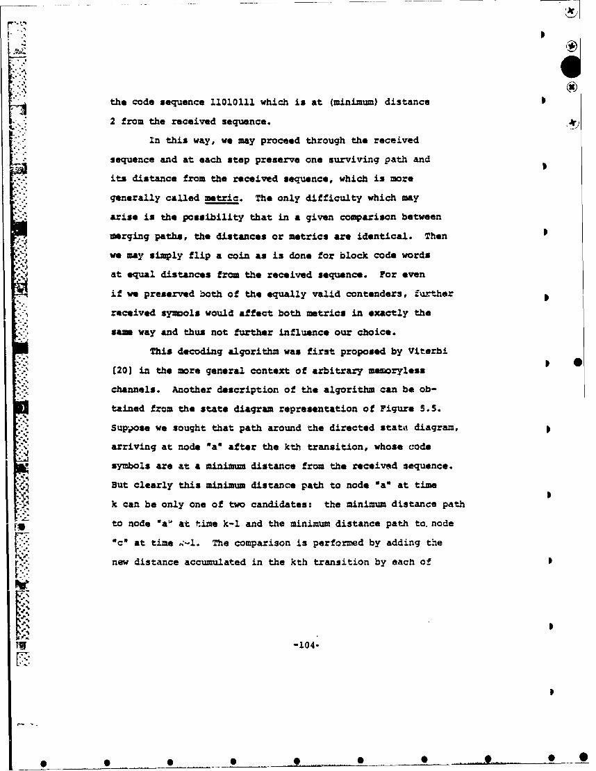
K (X
i' the code sequence 11010111 which is at (minimum) distance
2 from the received sequence.
In this way, we may proceed through the receivedsequence and at each step preserve one surviving path and
its distance from the received sequence, which is more
generally called metric. The only difficulty which may
arise is the possibility that in a given comparison between
merging paths, the distances or metrics are identical. Then
we may simply flip a coin as is done for block code words
at equal distances from the received sequence. For even
if we preserved both of the equally valid contenders, further
received symools would affect both metrics in exactly the
same way and thus not further influence our choice.
This decoding algorithm was first proposed by Viterbi
""20] in the more general context of arbitrary memoryless
channels. Another description of the algorithm can be ob-
tained from the state diagram representation of Figure 5.
SuFpose we sought that path around the directed stat&o diagram,
arriving at node *a* after the kth transition, whose code
symbols are at a minimum distance from the received sequence.
But clearly this minimum distance path to node "a" at time
- ~ k can be only one of two candidates: the minimum distance path
to node *a' at time k-i and the minimum distance path to. node
*c* at time ý-1. The comparison is performed by adding the
r.'. new distance accumulated in the kth transition by each of
-104-
0 O S S 0 0 0p I

these paths to their minimum distances (metrics) at time
k-i.
It appears thus th--t the state-diagram also re-
presents a system diagram for this decoder. With each
"node or state, we associate a storage register which
remembers the minimum distance path into the state after
each transition as well as a metric register which remembers
its (minimum) distance from the received sequence. Further-
more, comparisons are made at each step between the two
paths which lead into each node. Thus four comparators
must also be provided.
We deaer tho question of truncating the trellis and
thereby making a final decision on all bits beyond L branches
prior to the given branch until we have some additional pro-
porties of convolutional codes.
5.1.2 Distance Properties of Convolutional Codes
We continue to pursue the example of Fig•ure 5.2
for the sake of clarity; in the next section, we shall
Seasily generalize res-alts. As with linear block codes
there is no loss in generality in computing the distance
from the all zeros code word to all the other code words,
for this set of distances is the same as the set of distances
from any specific codeword to all the others.
Si For this purpose, we umay again use either the trellis
diagram or the state diagram. We first of all redraw the
71
'•' -l0S-
'.
S
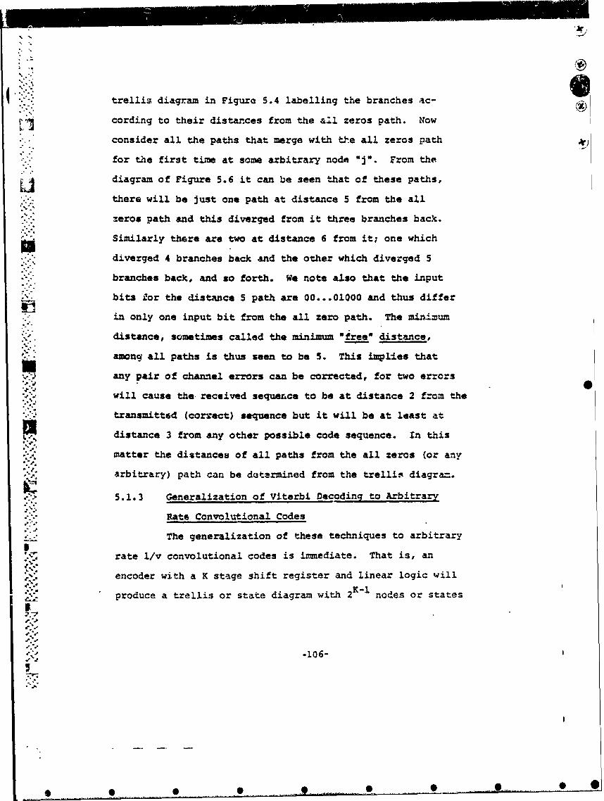
4 tr el elis diagram in Figure 5.4 labelling the branches ac-
cording to their distances from the all zeros path. Now
consider all the paths that merge with the all zeros path V
for the first time at some arbitrary node "j". From the
diagram of Figure 5.6 it can be seen that of these paths,
there will be just one path at distance 5 from the all
"zeros path and this diverged from it three branches back.
Similarly there are two at distance 6 from it; one which
diverged 4 branches back and the other which diverged 5
branches back, and so forth. We note also that the input
bits Zor the distance 5 path are 00...01000 and thus differ
in only one input bit from the all zero path. The min.imum
"distance, sometimes called the minimum *free* distance,
"among all paths is thus seen to be 5. This imptles that
any pair of channel errors can be corrected, for two errors
will cause the- received sequernce to be at distance 2 from the
"transmitted (correct) sequence but it will be at least at
distance 3 from any other possible code sequence. In this
matter the distances of all paths from the all zeros (or any
arbitrary) path can be detarmined from the trellis diagra=.
5.1.3 Generalization of Viterbi Decoding to Arbitrary
Rate Convolutional Codes
The generalization of these techniques to arbitrary
.• .rate 1/v convolutional codes is immediate. That is, an
encoder with a K stage shift register and linear logic will
produce a trellis or state diagram with 2 K- nodes or states
S""1-106-
F77 09.

Tine~0 °
' 2:...2
-
"0 0
10
Figure 5.6 Trellis diac~rarm labelled with distan.ces,on he all ----- s =ath.
S1%
.4..-
: .
"-'.:-
.--" " -I"
""" 107 " /I
-,2 " 2 .,
0• 0 0.0

and each branch will contain v code symbols. The rate
of this code is then
•" 1 bits,�v code symbol
The example pursued in the previous sections had rate
"R-1/2. The primary characteristic of rate 1/v codes is that
I only two branches exit from and enter each node.
-If rates other than I/v are desired, we must make b
greater than 1 where b is the number of bits shifted Lnto the
encoder at one time. An example for R-4 and rate R-2/3 is Shown
in Fiqure 5.7. its state diagram is shown in Figure 5.8.
It difiers from the binary-tree (b-1) representation
I. only in that each node is coign-cted to four other nodes,
and for general Ob, it will be connected r-c 2b nodes. Stilt
all the preceding techniques including the trellis and state
* diagram analysis are still applicable. it must be noted,
however, that the minimum distance decoder must make com-
parisons among all the paths entering each node at each
Slevel of the trellis and select one survivor out of 2
An interesting class of, in general, nonbLnary-tree
1 (b#l) convolutional codes is the unit-memory codes of Lee(21]. The memory of a convolutional code is defined as the
number of b-bit input groups from the last input group to
the oldest group that contributes to the present v outputs.S
.5
0 0 _ 00-0 0-

REPRODMJCFD AT GOVE RJ;A`T EXP.NSE
0®
.1
%4
S1•~Mdulo-2 Pdditio• Used •
o. ~Figure S. 7 K-4, R-2/3 encoder.
II
' -109"
! • .. . .. • .. .. . .• . . .. e .. . • . -• • .... . • . .. . .• ._ ... • .I

7 ------wo9w •.v, ,--s•z-
1 0
I@
IOI®
oco
I Figure 5.8 State diagram for code of Figure 5.7
... -110-
"0
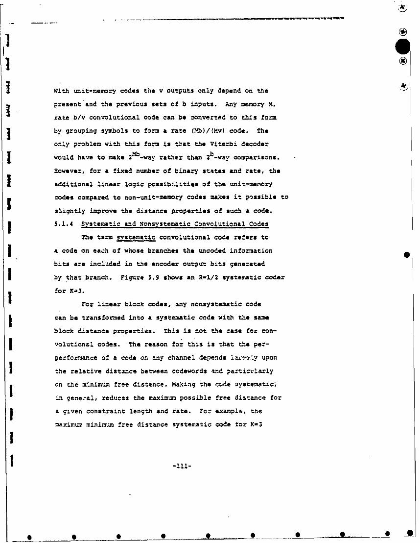
t0
With unit-memory codes the v outputs only depend on the
present and the previous sets of b inputs. Any memory M,
rate b/v convolutional code can be converted to this form
j by grouping symbols to form a rate (b)/(Mv) code. The
only problem with this form is that the Viterbi decoder
would have to make 2Mb-way rather than 2b-way comparisons.
However, for a fixed number of binary states and rate, the
I additional linear logic possibilities of the unit-memory
codes compared to non-unit-memory codes makes it possible to
slightly improve the distance properties of such a code.
1 5.1.4 Systematic and Nonsystematic Convolutional Codes
The term systematic convolutional code refers to
I a code on each of whose branches the uncoded information
bits are included in the encoder output bits generated
I by that branch. Figure 5.9 shows an R-1/2 systematic coder
I for K-3.
For linear block codes, any nonsystematic code
can be transformed into a systematic code with the same
block distance properties. This is not the case for con-
volutional codes. The reason for this is that the per-
performance of a code on any channel depends i-y upon
Sthe relative distance between codewords and paticvlarly
on the e.nimu- free distance. Making the code systematic>
in gene.al, reduces the maximum possible free distance for
a given constraint length and rate. For example, the
maximum minimum free distance systematic code for K-3I1 -111-
* . . e . . .. _ _. .. .. • .. 0.

-- I
p
It S
otput Input
_• • modulo-2
Addition
* 0
Figure 5.9 Systematic convolutional encoderfor K 3, R 1/2.
S
S
-112-
• • • • . • . . b• . ... .. • ... . _
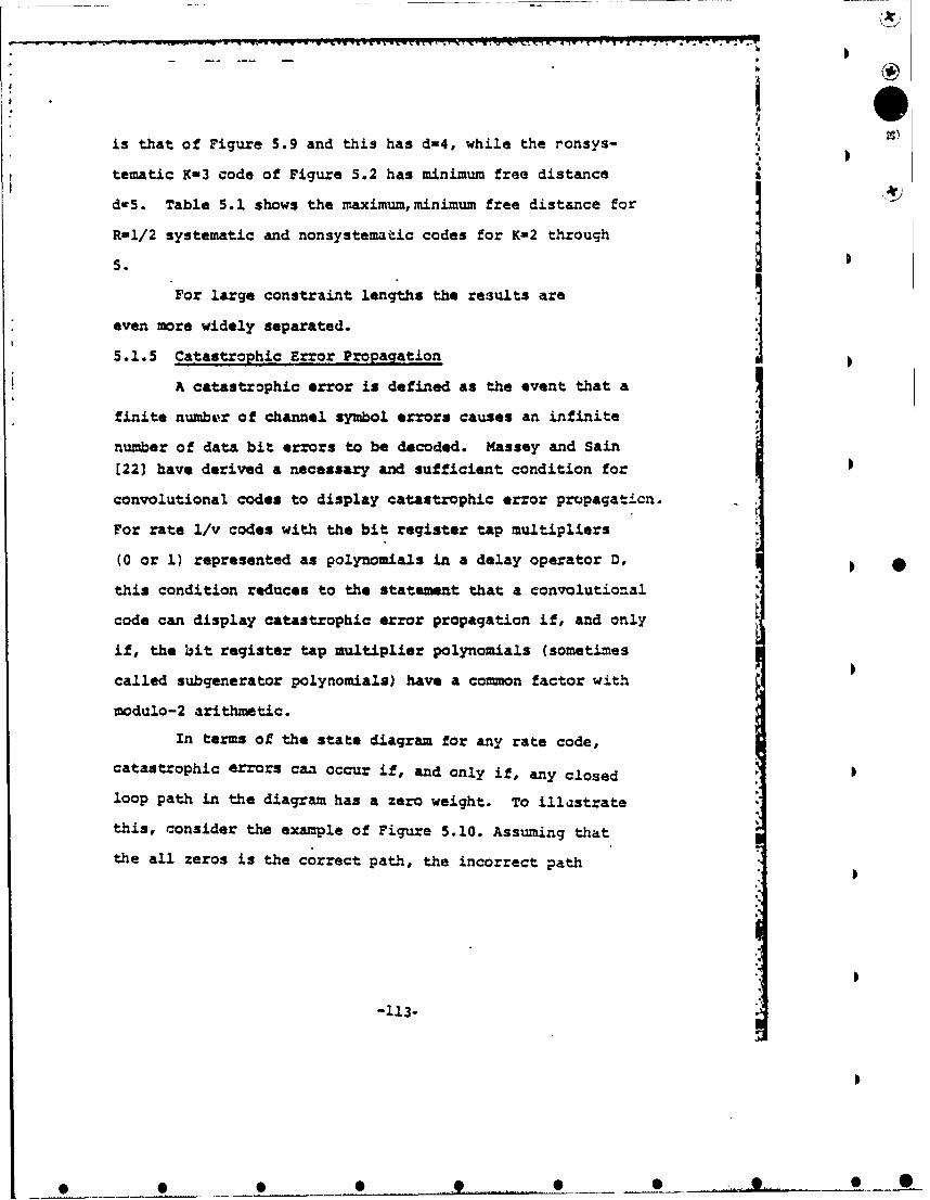
-' r-- .. w w~rrwrr- - -~------ * * I I *. . . * *.
O
is that of Figure 5.9 and this has d-4, while the ronsys-
tematic K-3 code of Figure 5.2 has minimum free distance
d-5. Table 5.1 shows the maximum,minimum free distance for
R-1/2 systematic and nonsystematic codes for K-2 through
5.
For large constraint lengths the results are
even more widely separated.
5.1.5 Catastrophic Error Propagation
A catastrophic error is defined as the event that a
finite numbier of channel symbol errors causes an infinite
number of data bit errors to be decoded. Massey and Sain[22] have derived a necessary and sufficient condition for
convolutional codes to display catastrophic e*or propagaticn.
For rate 1/v codes with the bit register tap multipliers
(0 or 1) represented as polynomials in a delay operator D,
this condition reduces to the statement that a convolutional
code can display catastrophic error propagation if, and only
if, the bit register tap multiplier polynomials (sometimes
called subgenerator polynomials) have a common factor with
modulo-2 arithmetic.
In terms of the state diagram for any rate code,
catastrophic errors caa occur if, and only if, any closed
loop path in the diagram has a zero weight. To illustrate
this, consider the example of Figure 5.10. Assuming that
the all zeros is the correct path, the incorrect path
-113-
• • • •

Maximum, Minimum Free Distance 1
K Systematic Nonsystematic
2 3 3
3 4 5
4 4 6
5 5 7
.able 5.1. Comparison of systematic and 5 0nonsystematic R-1/2 code distances.
1
S
IS•.. • . .5 . ..__ 0. .. . ... . . . ..

a- ,V.•
'0Input 00
01 1d
<-ouo!11 la1 01a I
Ezicod~0- Sae tiagram
b."
S':.
Figure 5.10 Coder dirplaying catastrophicerror propagation.
S.•
,a.
o'.5
•-.
-115-. ,

a b d d d c a has exactly 6 ones, no matter how many
times we go around the self.dioop d.• Thus, for a binary
"symmetric channel, for exampl*:",. four channel errors may
"cause us to choose this incorrect path or consequently make
an arbitrarily large number of bit errors (equal to two*-.• plus the number of times the self loop is traversed).
The necessary and sufficient condition of Massey and
Sain can also be used to show that the codA of Figure 5.10"
displays' catastrophxc error *propagation. The subgenerator
polynomials for this code are 0+1 and D2+1. Since
D2+1 - (D+l) (D+L) with modulo-2 arithmetic, both subgenerator
- polynomials have a comn factor of D+1. Therefore the code
displays catastrophic error propagation.
We observe also that for binary-tree (R-l/v) codes, 0
if each adder of the coder has an even number of connections,"then the self loop corresponding to the -all ones (data)
state will have zero weight and consequently the code will
be catastrophic.
The only advantage of.a systematic code is that it
can never be catastropaic, since each closed loop must
A,. contain at least one branch generated by a nonzero data bit
*5.* and thus have a nonzero code symbol. Still, it can be
"-116-
* * * * ..... e .. ..... . • ... .,.......

S shown that only a small fraction of nonsystematic codes
are catastrophic (231. We note further that if catastrophic *rj
- errors are ignored, nonsystematic codes with even larger
free distance than those of Table 5.1 exist.
5.1.6 Generalization of Viterbi Decoding to Soft Quan-
"Ky• tized Channels.
To describ3 how the Viterbi decoding algorithm
operates with soft quantization consider the biphase (00 or
180") modulated additive white Gaussian noise channel.
Then in addition to the sign of the demodulator output an
indication of its magnitude is provided. The first step
"is to assign metri(. values to each of the possible outpit
"intervals under the hypothesis that the 0 phase was used
and that the 1800 phase was used. A comn choice is to
use integer metric* which for a positive (0").hypothesisassigns a 00 symbol metric value to the most negative
demodulator output interval and unity increasing metric
values to the progressively more positive demodulator inter-vals. For 3-bit quantization the metrics would go from
0 to 7. With the negative (180*) hypothesis metrics
decreasing from 7 to 0 are used.
The metrics for any branch or path are computed by
summing the corresponding symbol metrics with the set of'
"metrics to use (positive or negative hypothesis) det.ermined
-117-
• . ,. _
r
by the polarity of the test channel symbol. Then the metrics
of remerging paths are compared and the path with the small-
est metric is eliminated.
Note that the path metrics as described he:e would 0
"-- continually increase. Hbwever, since the metrics are used
in comparison, only their relative differences are required.
So some amount can be occasionally subtracted from all of
the path metrics to keep them within a certain range.
"Computer simulations and measurements of hardware
systems for a wide variety of codes and channels have
shown that the differences in the-Eb/No ratios required to"achieve a given error rate for various numbers of quan-
tization intervals with the integer metrics described here
(and in fact most reasonable metric choices) are almost S 0
exactly as estimateA in Section 3.2 based on operation at,-.-.R
5.1.7 Path Mowry Truncation"Another problem which arises in the implementation
oZ a Viterbi decoder is the length of the path history
which must be stored. In our previous discussion we
ignored this important point and therefore Lmplicitly
assumed that all past data would be stored. A final
decision can be made by forcing the coder into a known
IFI
P'... -118-
°° A

(all zeros) state, but this is totally impractical for
long data sequences, for it requires storage of the entire
trellis memory for each state. Suppose we truncate the
path memories after L bits (branches) have been accumulated,
by comparing all 2 metrics for a maximum and deciding
"on the bit corresponding to that path (out of 2) with the
highest metric L branches forward. If L is several times
as large as K, the additional bit errors introduced in this
way are very few. It can be shown that the additional error
"probability due to path truncation, based on the largest
"path metric L branches beyond where the decision is to be
made, is of the order of a block coding error for a code of
w block length L bits. Both theory and simulation have shown
that by making L four to five times as large as the codt
constraint length K, we can ensure that such additional
errors have only a slight affect on the overall bit error
probability.
Of course, basing the decision upon the maximum
metric L branches forward may require a costly im-plemen-
tation to compare all 2 state metrics. Other decision
techniques, based on majority polling and metric overflow
monitoring, are much less costly and yield the same or
better performance when L is increased slightly.
0-119-
• • .. . . . ...

0O
5.1.8 Code Selection
The linear logic for a convolutional code isI0
usually selected based on the code distance properties
as discussed in Section 5.1.2. The first criterion is to
select a code (linear logic) that does not have catastro-
phic error propagation (see Section 5.1.5) and that has
t-he maximum possible free distance for the given rate and
constraint length. Then the number of paths or dyer- S
saries at the free distance or if the bit error prob-
ability in the performance measure, the total number of
information bit errors represented by the adversaries at 0
the free distance should be minimized. This selection pro-
cedure can be further refined by considering the number of
adversaries or information bit errors at the free distance
plus 1, plus 2, etc. until only one code or class of codes
remains. A listing of R-1/2 1-3 to 9 and R-1/3 K-3, to 8codes selected based on this criterion is given in Table
5.2, (Reference 24, but note K-7, R- 1/3 correction).. 0
The R-l/v constraint length T codes in this table are
specified in terms of v K-digit sequences. The i th
digit (0 or 1) in the j th sequlance specifies the tapmultiplier in determining the contribution to the j th
branch output due to the symbol in the i th encoder re-
gister stage. The total j th output is the modulo-2 sum
of the v individual contributions. P
-120- 0
0

I 'A
"Rate Constraint Length Code
1/2 3 111101
S1/2 4 11111/21101
1/2 5 1110110011
1/2 6 111101101011
1/2 7 11110011011011
1/2 8 1111100110100111
"91/ 9 111101011"101110001
1/3 3 1il111
S~1101• 1011
1/3 111111101110010101
1/3 a 111101.[ 101011! 100111
1I/3 7 11110011110101
1/3 1111011111011001
S~10010101
Table S.2 Optimum short constraint lengthR-II/-2 and 1/3 convolutional codes.
-121.

Other codes which achieve the maximum free distance
but do not necessarily have the minimum number of bit errors
as described above, are given in Reference 25 for R-1/2, 1/3
and 1/4 ccdes and in Reference 26 for R-2/3 and 3/4 codes.
5.1.9 Computer Simulation Performance Results
One of the main methods of determining the per-
formance of convolutional coding systems is by computer
simulation. Such simulations are especially helpful in
determining the error rate performance at higher error rates
where analytical bounding techniques are not very tight and
where the error probabilities can be estimated with a reason-
"able amounu of computer time.
Sometimes the all zero information input sequence
is assumed, but when only a few quantization intervals ) •
are used it is best to use random data to avoid biasing the
results due to the method of resolving metric comparison
ties. The advantage of using the all zuro sequence is that
no encoder is necessary since the encoded sequence will
still be all zeros and determining the error rate reducesto determining the fraction of nonzero decoder outputs.
The quantized received data sequence is generated bymodifying the enccded sequence according to the channel
S~transition probability diagram (see Figure 3.6 and 3.9).
Once the quantized received sequence is generated a Viterbi
-122-
0 0 0 0 • --

". decoder identical to a hardware implementation can be
programed. The error rate is determined by comparing
-' tb. Viterbi decoder output with the delayed information
sequence.
Figures 5.11, 5.12, and 5.13 show the bit error
probability performance of K-7 R- 1/2, K-7 R- 1/3, and
K-9 R- 3/4 convolutional coding systems on an additive
white Gaussian noise channel with hard and 3-bit soft
quantization. These simulation results have also been
verified by measurements on hardware systems. The upper
bounds shown in these figures are discussed in the next
two sections. Figures 5.11 through 5.13 again illustrate
the advantages of soft quantization discussed in Section
3.2. The K-7 R- 1/2 code used for Figure 5.11. is the
optimum code given in Table 5.2 and the K-7 R- 1/3 •
code used for Figure 5.12, while not optimum in the dis-
tance sense used in Table 5.2, achieves a bit error prob-
ability virtually equivalent to (in fact slightly better
than) the code of [25] in the range of error probabilities
shown.
The R- 3/4 code used for Figure 5.13 is not the best
possible code. At a bit error probability of 10-5 ocher
codes superior (i.e., with smaller bit error probability)
to this code and the code of (261 can achieve about .4 dB
E./No improvement over that shown in Figure 5.13. The 0
-123--

10-1
10-2
\Hard Quan-> 91 0 "
t i z a t i o n
- Bound
\ \ tization0o4 1 Simulation
04 No Quark-
LI tization Bound'a3-Bit 5 0
QuantizationSimulation3-Bit (T-.S)QuantizationBound
10%
I x
\I-I
10-61
1 2 3 4 5 6 7 8Eb/N 0in dB
Figure 5.11 Bit error probability versus E /Nperformance of a K=7, R- 1/2 cn-volutional coding system with BPSKmodulation and an AWGN channel.
-124-
0I

10-2
', 'I I
I --
' ®
Hard10-"
"4 ~Bound
$4 zationSlimu-
I lation10W - No Quanti-a 1 zation Bound\
3-it 5)\Quantization Slimu-
S\ \ .'- zaation
3-Bit (T-.5)Quantization Bound
10 6t
0 1 2 3 4
Eb/No in dB;
Figure 5.12 Bit error probability versus E /Noperformance of a K-7, R- 1/3\volutional coding system with BPSKodulation and an AWGN channel.
-125-
10-5 • \
\ \ \~ 0
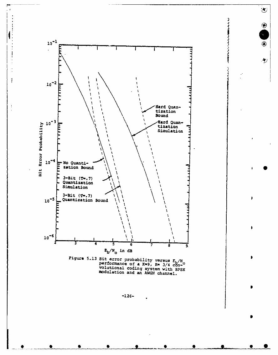
10-2 ==_ _•__I I
-\e t12ation
Bound
1 10,,,,-Hard Quan-.0 j tization
Simulation
.0
.0o4 10 1-N-uni
0 zation Bound \-4
3-Bit (Ta.7)Quantization I ~Simulationk
3-Bit (Tw. 7)10-5 Quantization Boud X k
1 -A
40- \ \ 7 9
Eb/No in dFigur-e 5.13 Bit error Drobability versus F IN
performance of a Ka9, Ru 3/4 cAn-°Volutional coding system with SPSKmodulation and an AWGN channel.
-126-

reason for giving the performance of this particular code as
is th5 . the encoder/decoder for this K-9 R- 3/4 code
and the K-7 R- 1/2 code have been implemented as a switch-
selectable, option in A single unit with only a few more
standard integrated circuit chips than are required for
the single KX7 R- 1/2 encoder/decoder.
Simulation results have also been obtainer
many other codes on the additive white Gaussian noise
chaanel [271. The results show that for rate 1/2 codes Cl
each increment increase in the constraint length in the
range K-3 to 8 provides an approximate .4 to .5 dB E /%
improvement at a bit error rate of 10.
The coding gain is just the difference between
the Eb/NO required for a particular error rate without I.
coding and with coding. Figure 5.14 shows the 3-bit quan-
tization coding gain for the codes of Figure 5.11. 5.12,
and 5.13.
The hard quantization curves of Figure 5.11, 5.12,
and 5.13 can also be expressed in terms of the channel
error rate. The results are given in Figure 5.15. This
figure can be used to obtain the performance of these hard Kquantized coding systems for different memoryless modu- LV
lation and channel types using the bit error prcbabtlity.
curves of Section 3.1. Just treat the curves of Section
r.1
-127- •
• • qp • • -. .•• •
• .. .. . 0.. . . . . ...

41 44
V r.
0i
I= 4
-4
r-44
Aj $4
M~44
'44
.ý4
0n
9P UT .4V! BUTO
-128-

102
I
102 # -
10-4
So~0
10-51.4
10" - 2 10-310
Channel Error Probability
Figure 5.15 Bit error probability versus -channel error rate performanceof several convolutional coding 0systems.
-12p-129-

3.1 as the channel symbol error probability versus the
channel symbol energy-to-noise ratio. The coded system
information bit energy-to-noise ratio is then
(5.2)N R N
0 0
As mentioned previously, interleaving can be used to make
the channel appear to be memoryless.
For example, on an independent Rayleigh fading
channel with binary FSI a X-7, R- 1/2, L-4 diversity sys-
tem with hard quantization requires %/NO - 15.1 dB for
l ab 10"5. This is 2.8 d.B better than the optimi-m di--.
versity (L=16) uncoded system (see Figure 3.5)
for this channel and 3.8 dB better than an uncoded system
with the same 8 channel bits per information bit.
Figure 5.16 shows the 2imulated additive white Gaus-
sian noise channel performance of a Viterbi-decoded con-
volutional codin. 3ystem ideally suited for bandlimited
"situations (36]. This system consists of a K-8, R- 2/3
convolutional code with an octal-PSI modem. This system
'-- has the same bandwidth requirements for a given data rate
as an uncoded QPSK system. Such a 3ystam is sometim:
referred to as a *unity bandwidth expansion. ceding system".
Figure 5.16 also shows the effects of Viterbi decoder
path memory truncation for this system.
-130-
40- .

", "-1
" ,-""• 10 3 I i
0Er. ,1
inma y 32 bi:.,
I'bm..N~oxy - 64 bit.s
• • 10"-
3-. 4 . 1
I -4
,°~
E I.No in d
0
•'•Figure 5.16 Perfs.,rmance of the modulation and•'.'-coding system wioth a rate 2/3, con-i",". traint length 8, Viterbi-decodedi•contolutional code and anoctal-PSK.'. modem for several path length memories.
14131-
AS

D
Figure 5.17 gives the simulation bit error probability
performance of a K-7 R- 1/2 convolutional coding system
with DBPSK modulation on an additive white Gaussian noise 4
channel. As expected from the results of Section 3.2.2.3
•i. ~ the performance of this system is considerably inferior
"to the same coding system and channel with BPSK modulation.
Sometimes the message rather than thi bit error
- probability is the performance measure. A simple upperSI
"bound on the message error probability for an M-bit message
e-? is Just N times the bit error probability. However, since
the output errors in an Viterbi-decoded convolutional coding
system tend to occur in bursts, this bound is somewhat
pessimistic. To characterize the bursts out of a Viterbi-
decoder, define an error burst to be the sequence of in-
formation symbols from the first error to the last error
"during which the path choosen by the Viterbi decoder through
"- the trellis is not merged with the correct path. During
this burst some of the symbols may be correct, but for R- 1/v
codes the correct subsequeiices in the burst are less thanK-i bits in length because longer sequence would cause
.1 the path to remerge with the correct path. Note that since
the last K-i bits of the unmerged span must be correct
for the path to remerge with the correct path, the burst"",3.
'.-,- 32
-t2
• • •• • •• •

10
x
"C..
.0 Hard Quazntii.ation.0
10
4". nW3".-. (T7)
"4 Quantizationi
4
)-:.-
10-2
3 4 5 6 7 8 9 10
Figutre 5.17 Bit error prob)biity"I versus 111/4 performance of a
a K-7, R1/9 convolutional
P""
coding system with DBPSKmodulation and an AWGN channel.
-133-
_ * 0,...,0lO- _ !_____!_!_

length is K-I luss than the length of the unmerged span.
"Tables 5.3 and 5.4 give error burst statistics for the
K-7 R- 1/2 system with 3-bit and hard quantization, res-
pectively. The event error probability (i.e., the event
of the start of an error burst) is the bit error prob-
abi-lity divided by the average number of bit errors per
bust. Then a better upper bound on the 1-bit message
error. probability is 4 times the event error probability5.1.10 Analytical Performance TechniqugRi with No Quan-
tization
"The basic method of analytically determining the
performance of noncatastrophic Viterbi-decoded convolutional
coding systems is with the generating function approach of
Viterbi [281. With this technique the first step is to
determine a generating function T(D,N,L) which d'escribes
all the different paths which could be compared with the
correct path assuming the all zeros message is used. In the 0
infinite expansion o! T(D,N,L) the power of D in the terms
represents the number of channel symbols in which the path
differs from the correct (all zero) path, the power of N
represents the number of information bit errors in the path,
-134-
II
* _

I
/
Uw
Average Error Burst Average Number of
"Eb/No Length in Bits Errors per Burst
1.0 17.3 12.1
2.0 10.9 5.9
3.0 7.6 4.3
4.0 6.2 3.8
Table 5,3 Error burst statistics for K-7 R- 1/2system with 3-bit quantization.
-135-
. • .. .. ...... • .. . . . 0 . . . . 0 . .. . .• .. 0 . . .. . .. .. 0- b .. .. .. 0 .. .

E"/No Average Error Burst Average Number of
b o Length in Bits Errors per Burst
4.0 13.3 7.8
5.0 9.9 5.5
6.0 7.9 4.5
Table 5.4 Error burst statistics for a --7 R- 1/2sy. .em with hard quantiation.
-136-
• 9 o ._O
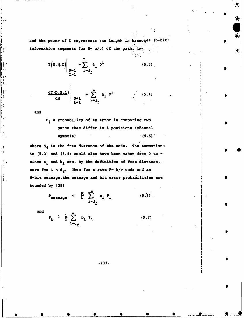
and the power of L reprosents the length in branches (b-bit) 0
information segments for R- b/v) of the path'-' Let ..
N-i i-drL-1
VdT(D,NeL) - b Di (3.4) K10- i-df
and
P i Probability of an error in comparing two
paths that differ in i positions (channel
symbols) (5.5)'
where df is the free distance of the code. The. summations
in (5.3) and (5.4) could also have been taken from 0 to *
since ai and bi ara, by the definition of free distance,.
zero for i < d . Then for a rate R- b/v code and an
1-bit message,tht message and bit error probabilities are
bounded by [281
Pmessage < a Pi (5.6)imdf
and
P b bi Pi(S7
i-dff
D
-137-

To illustrate this technique and to provide some
rational for (5.6) and (5.7) consider te K-3, R- 1/2 codea
of Figure 5.2. The first step is to determine the generating
function. To do this refer to the modified state diagram
of Figure 5.18. This modified state diagram was obtained
from the state diagram of Figure 5.5 with the all zero
state split into an initial and final state, the all zero
state self loop omitted, and the branches marked with the
branch generating functions. The path generating functions
of all the paths that can be compared with the correct
(zero) path are represented in this diagram by all the
possible paths from the initial all zero state to the final
all zero state. These paths can be expressed as the trans-
fer function of the diagram. For this example the result
is
D5N 3
T(D,N,L - NL3l"-1NLDNLZ (5.8)
D 5 NL 3+06 2(45) +07N31 L542L 6 +L 7) +..
Equation 5.8 shows that among the adversaries to the
correct (all zero) path there is one path of weight 5, and
it is three branches long and results in one bit error.
There are two paths of weight 6, one of length 4 and one of
length 5, and both result in two bit errors, etc. The
message error probability can then be bounded by the prob-
baility of an error in any set of ccmparisons times the
-13I
-13 8-
I
0 0 0 0. 0 . . • . .. 0 .. . • . ... . . . . •

DND I S®
i6\*
DNLOWL I
O2NL
Figure 5.18 Modified state diagram for the K-3,R-1/2 convolutional code of Figure 5.2.
-139-
___________ e
t•. . . . .. •0
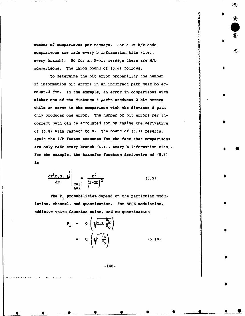
-I
lox
number of comparisons per message. For a R- b/v code qcompax-ions are made every b information bits (i.e.,
every branch). So for ai M-bit message there are M/b
comparisons. The union bound of (5.6) follows.
To determine the bit error probability the number
of information bit errors in an incorrect path must be ac-
countra fnr. In the example, an error in comparisons with
either one of the t.istance 6 pzthq produces 2 bit errors
while an error in the comparison with the distance 5 pcL
only produces one error. The number of bit errors per in-
correct path can be accounted for by taking the derivative
of (5.8) with respect to N. The bound of (5.7) results.
Again the 1/b factor accounts for the fact that comparisons
are only made every branch (i.e., every b information bits). * *For the example, the transfer function derivative of (5.4)
is
dT(D,N, L) D-dN N_ " '2DI 2(5.9)
The Pi probabilities depend on the particular modu-
lation, channel, and quantization. For BPSK modulation, P
additive white Gaussian noise, and no quantization
p-i-140-
(5.10)
-140-

If~r this R- 1/2 example where
2L
x)p f')dy (5.11)
Using the bound
, i > df (5.12)
the message and bit error probability bounds for this
example become
P MQ 0~Pmessage 1- x (5. 13)
and
P - 2(5.14)
for Zb/No ratios large enough so that the denominator of
(5.13) is positive.
This example illustrates the two main problems
with this technique: that of determining the generating
function and that of computing or bounding Pi. For small
error rates only the first few terms in the summations
of (5.6) and (5.7) contribute significantly to the bounds.
So a good method of using this technique is to use exact
14
-141-

00
expresaions or tight bounds for the P of the first ,)
few terms and then to b6und th., remaining Pi by bounds
of the form
Pi CODoi (5.15)
where C0 and Da re quantities which do not depend on
i. In the ezample above we used
C0- dfR 17- (5.1d)
and
for i '_df + .1.
With bounds of the form of (5.15) the transfer
function only has to be evaluated for a particular D-D0 .
This can be accomplished with a computer using the state
equations [291.
S- A S +_ (B.18)
T (DI,,L) - C S (5.19)
where S is a column vector whose components are equal
to the branch transfer functions from the all zero-state
to each of the nonzero states, A is a matrix whose com-
-142-
SAt..

ponenta aij are :he branch transfer functions from the
j th to the i th nonzero state, B is a column vector
whose components are the branch transfer functions fromthe initial zero state to the i th nonzero state, and
C is a row vector whose components are the branch transfer
Eunctions from the i th nonzero state to the final zero
state.
A computer program has bee3n written (29] to compute
(5.7) for specific D values. This no-quantization bound
is compared with simulation results in Figures 5.11, 5.12,
izd 5.13.
Figures 5.19, 5.20, 5.21, 5.22 and 5.23 give this bit
error probability bound verss Eb/No for R- 1/2, 1/3, 1/4, 2/3
and 3/4 codes, respectively, of (251, and [26] with biphase
BPSK modulation, additive white Gaussian noise and no
quantization. With 3-bit quantization an additional .25 d3
is required and with hard quantization an additional 2 dB
is required.
The somewhat poor peformance of the K-7, R-1/4
code of Figure 5.21 is due to the large leading b, coef-
ficient (i.e., bd in Equation 5.4) of that code. A
K-7, R-1/4 code with a smaller leading coefficient and
the same maximum free distance can probably be found.
5.1.11 Analytical Performance Techniques with Quantization
The bounding technique of Section 5.1.10 can als:ý be
used on quantized channels. Let D(Z) be a polynomial des-I-
crJbing the metric differences that could occur in com-
paring an incorrect path with the correct (zero) path.
-143-
___ S0 0 ___

K-3 to 9 codes IromTable 5.2
10 b10 code from Refe-
10 -4 ,-,dw Ir6, d f UL
10\
I.\ P4
S10
0
K-7, d f 10
I-I
K0ing, d flO 10
K=9, df=12
AX-10, df-42
3.0 3.5 4.0 4.5 5.0 5.5 6.0 6.5
Eb/No in dB;
Figure 5.19 Bit *rr-.r probability versus EF/Nperform.once bat'nds for several 1NR-'1/2 Vitirbi-decoded convolutionalcc;ding systems with no quantization.
-144-

I - I
Ký3, d as8
r-?•10-3
,"."K-4, d -10
SK -5, d f-12
•. //Ka6 d df-13
10-4
10
• Li
0 14Sl°'e K-:e, d.l is\
1-1 X., af2n0
-K3,4,5,6 and 8 codefrom Table 5.2
K-7,9 and 10 codes10" . from Reference 25
io
2.5 3.0 3.5 4.0 4.5 S.0 5.5 6.0
Figure 5.20 Bit error probability versus Eb/Noperformance bounds for several"R-1/3 Viterbi-decoded convolutional'-oding systems with no quantization.
-145-
• • . .. • . .. • .... e . ... . •.. ••. .. .. . ..
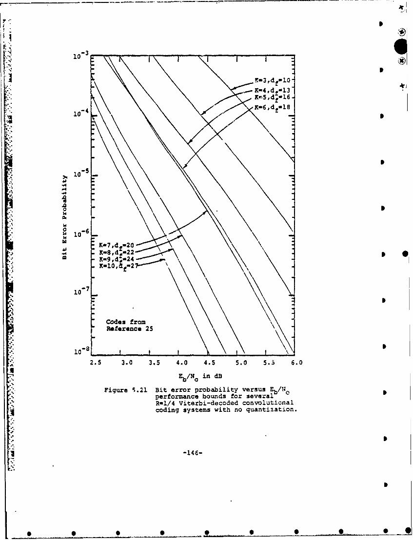
3-3,d 010i-N;
-4, d df=13K-5 1df01 6
• -i • " K67,d-18
0 \
10-4 fV.4
10
"4Codes fro22
10 .-7m2-~
4 ~Codes fromReference 25
II 108
A2.5 3.0 3.5 4.0 4.5 5.0 5.3 6.0
-b/No in dB
Figure 5.21 Bit error probability versus Eb/Noperformance bounds for severalR-1/4 Viterbi-decoded convolutionalcoding systems with no quantization.
U• -146-
%"I
0 0 00 __0 0

3I
10 a
X-4, d =3
5II
10" a
•-4" "K -6, df=S
">4
-.. 10 -
-- * IA K-6, dr= US
-4.4 J 4I•- - f
K-8, d =7
-7.. K =-8,. d f=710N X-9, d f 8 -
Codes fromReference 26
10"4.0 4.5 5.0 5.5 6.0 6.5 7.0 7.5
Figure 5.22 Bit error probability versus ,/N_performance bounds for severalR-2/3 Viterbi-decoded convolutionalcoding systems with no quantization.
-147-

3I
Snun milm IIii lllIIlnl
10
p 106, d f=4 I
-4- K-8, dfin5
P" f
.0
* I
S10-5 f "
ihu"l \ -, ,7r-
1=I12, df=8
Codes fromReference 26 \,
a. - ,i ~ __'____._. I
4.0 4.5 5.0 5.5 6.0 6.5 7.0 7.5iI
Lb/No in dB
Figure 5.23 Bit error probabi:ity versus Eb/N 0performance bounds for several R-'3/4Vitecbi-decoded convolutional codingsystems with no quantization.
-148-
-0S

N!
In particular let the powers of Z represent the possible
branch metric differences between the incorrect and the
correct branch metrics and the coefficient of that term
the probability of that metric diffe:ence. With n quan-
tization Jntervals
D(Z) -PiJ zMPj Mj (5. 20)i=O j-0
where pLj is the probability that the incorrect channel symbol
mettric is M~)and the correct channel symbol mnetric is M
If two paths differsed in only one channel symbol,
a Viterbi decoder would make an error in compariag the
two if the incorrect path metric exceed the correct path
metric. So
P1 " (15.21
where
S=m of the coefficients of the
tU(z)1t (positive power terms of OIWZ)
+ 1 (oefficient of the zero power)term of D(Z) (5.22)
The 1/2 factor for the coefficient of the zero power term
i is to resolve ties randomly. If the paths being compared
-149-
0 0 09 S ___
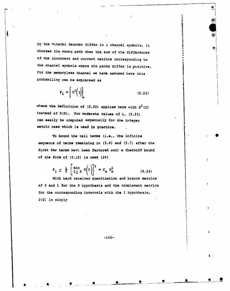
4 Iby the Viterbi decoder differ in i channel symbols, it
chooses the wrong path when the sum of the differences
of the incorrect and correct metrics corresponding to
the channel symbols where the paths differ is pcsitive.For the memoryless channel we have assumed here this
probability can be expreised as
P f iZ)}4 (5.23)
where the definition of (5.22) applies here with D()
instead of D(Z). For moderate values ofti, (5.23)
can easily be computed especially for the i.teger
metric case which is used iA practice.
To bound the tail terms (i.e., the infinite •
sequence of terms remaining in (5.6) and (5.7) after the
first few terms hav-- been factored out) a Chernoff bound
of the form of (5.15) is used 1291
P I [ ra~~in \1i - C-- O (5.24)
With hard receiver quantization and branch metrics
of 0 and 1 for the 0 hypothesis and the complement metrics
for the corresponding intervals with the 1 hypothesis,
D(Z) is simply
-150-

A(z) -(l-P) Z- pZ (5.25)
"" where p is the probability of a channel symbol error.
* The bound of (5.24) becomes
IiPi -- (5.26)
This bound is compa.ve; with simulated results with
" 3-bit quantization in Figures 5.11 5.12, and 5.13.
These figures show that, as expected, at high error rates
this union bounding technique is not useful, but for small
error rates it is vary tight. Similar Fesults have been
observed for 6thee codes.
The first few coefficients of the bounds of (5.6) and
(5.7) for the codes of Figures 5.11, 5.12 and 5.13 are
given in Table 5.5 [24].
5.1.12 Node Synchronization and Phase Ambiguity Resolution
-ecause of the inherent continuity involved in
convolutional coding, code synchronization at the receiver
is usual17' much simpler than in the case of block codes.
For convolutional decoding techniques involving a fixed
number of computations per bit decoded, such as Viterbi
decoding, the decoder initially makes an arbitrary guess
of the encoder state to start decoding. If the guess is
incorrect, the decoder will output several bits or, at
most, tens of bits of unreliable data before assuming
-151-

iI
K-7, R- 1/2 K-7, R- 1/3 K-9, R- 3/4df- 10 code of dr- 14 code of d US code ofFigure 5.11 Figure 3.12 Figure 5.1J3Distance
ai bi ai . bi ai bi
5 0 0 0 0 8 426 0 0 0 0 201
7 0 0 0 0
8 0 0o0 0
9 0 0 0 0
10 11 36 0 0
11 0 0 0 0
12 38 211 0 0
13 0 0 0 0
14 193 1404 1 1
15 0 0 0 0
16 1331 L1633 7 20
17 0 0 0 0
18 11 5319 0 0
20 3S 184
21 0 0
.IITable 5.5 Upper bound coefficients of (5.6) and
(5.7).
-±52-

II
steady state reliable operation. Thus, the block syn-
chronization problem does not really exist. There remains jthe problem of node synchronization and, depending upon
the mod'ilation-demodulation technique used, the problem
of phase ambiguity resolution. For a rate b/v code, there
are v code symbols on each branch in the code tree. Node
synchronization is obtained when the decoder has knowledge
of which sets of v symbols in the received symbol st:eam
belonq to the same branch. In a purely serial received
stream, this is a I in v ambiguity.
In addition, modems using biphase or quadriphase
PSK with suppressed carriers derive a phase reference for
coherent demodulation from a squaring or fourth power
phase lock loop or its equivalent. This Litroduces am- -
biguities in that the squaring loop is stable .-n the
in-phase and 1800 out of phase positions, and the 4th
power lomp is, in addition, stable at + 901 from the
in-phase position.
Viterbi decoders have been implemented which
maintain node and biphase or quadriphase PSK phase syn-
chronization completely within the decoder. One way to
resolve 1800 phase ambiguities is to use a code which is
transparent to 1800 phase flips, precode the data dif-
ferentially and lise differential decoding. A transparent
code has the property that the bit-by-bit complem-ent of
-153-

0*
a codeword is also a codeword. Such a code must have an
odd number of taps on each of its encoder rnod-2 adders.
This insures that if a given data sequence genezates a
certain codeword, its complement will generate the comple-
mentary code word.
If the received data is complemented due to a 1800
phase reversal, it will still look like a codeword to the
decoder, and will likely be decoded into the complement
of the correct data sequence. Now decoding to the com-
plement of the sequence input to the encoder is no pro-
blem if the data was precoded differentially. This
means thaý. information is contained in the occurrence *or non-occurrence of transitions in the encoded output
sequence rather than the absolute sequence itself. These
transitions occur in the same places even if the decodad
sequence is complemented.
The major fault with this scheme is that when
an isolated bit error occurs in the decoder output, it
causes two differentially deco'ed errors, since two trans-
itions are changed. At first glance, this would seem to
indicate a doubling of the output bit error rate. In fact,
I
.154-
S.. . 0 . .. .... • . . . .. . O . . . . •. * . ..... • • • .. . • . .. ...... qb• . . ......... • ... .

0
this doubling does not occur because errors typically oc-
cut in shdrt bursts. Two adjacent bit errors, for instance
cause only two differentially decoded bit errors. This
indicates the possibility of only a small increase in bit
exror rate with diffarential encoding-decoding.
In practice this is the case. For the K-7, R-1/2
transparent code of Figure 5.11, using differential encoding-
decoding causes an Eb/NO loss of less than .1 dB for bit
error probabilities in the range from 10- to 10-6.
Another method of resolving node or phase ambiguities
is to monitor the metrics and to change the node or phase
reference when unsatisfactory (very noisy channel) operation
is detected. This and the preceeding technique have been N 0implemented in hardware systems.
5.1.13 Quantization Threshold Levels
With soft receiver quantization the receiver must
have an automatic gain control (AGC) circuit to maintain
the best quantization threshold levels. Throughout this
report we use a uniform quantization. With 0° or 180*
biphase modulation and N-bit quantization the quantization 0
threshold levels are at 0, + T, :t 2T, ... , # (2 l-l)T. 0-
With additive white Gaussian noise, rate 1/2 coding,
and 3-bit quantization (N-3) the best choice of T is about
.5 times the standard deviation of the random variable to
¶0
-155-
J ,
• • • • 9 • ~ ~ ~ ~~ •_.... 0............•.... O

* *
be quantized, i.e., .5 Ni,/2. So an estimate of the
noise level is required.
Figure 5.24 shows the decradation resulting
from an error in-the measureiaent of N for the XQ-7, R- 1/2
convolutional code at a bit error 'ate oZ 2X10 5 . This
figure shows that this system is not every sensitive to
small AGC variations. For bit err-... rates of from 10"1
to 10-5 less than a .1 dB larger Eb/No ratio is required
to maintain the error rate performance due to up to + 3 dB
errors in the measurement of N0 for this code. Similar re-
sults have also been obtained for other Viterbi-decoded
convolutional coding systems.
5.1.14 Implementation Considerations
The main factors governing the implementation
complexity of a Viterbi decoder are the number of state
variables (i.e., K-b for R- b/v) and the speed. The
K-7, Ra 1/2 encoder/dacoder with internal node and phase
ambiguity synchronization has been implemented with 55 T.L
IC chips. This implementation performs the Viterbi decoder
comparisons mostly in serial and is capable of operating
at any information bit rate up to 100 Kbps. Eigher data
rates can be obtained by performing the comparisons in
parallel. Using such a parallel implementation the same
K-7, R- 1/2 encoder/decoder with synchronization capable D
of operating at information bit rates of up to 10 Mbps
has been implemented with about 250 IC chips.
-
-156-
0 __ _ - - - -- ' - -

1.0-
-4
*' 0.5"
O-4
S0.0C
-9 -6 -3 0 +3 +6 +9
Erzro in AGC Measurement of NO in dB
Figure S.24 Increa._ in Eb/N 0 .required to maintain a2 X 10 bit error rate versu.v error in AGCmeasurement of Eb/"o for a i0h7, R-1/2 code.
!I
-157-
imI
9 __
In -T.neral, increasing the number of state variables
by one ap~roximately doubles the implementation complexity
of a Viterbi decoder that purforms comparisons in parallel
and increases the implementation complexity of a serial
type decoder by somewhat less than a factor of two.
At low data rates Viterbi decoders can be implemented
"with microprocessors. However, unless the microprocessor
is also required for other funct..ons, a single decoder of
the comoiex~ty of a K-7, R- 1/2 code can presently be
implemented morn economically in hardiare. One application
• .'where a microprocessor irplementation may be preferable tc
"a hardware implementation is where several slow speed, short
constraint length deccders are r"qui'ed, such as in some
multiple acceas systems.
Other factors that effect Viterbi decoder implemen-
tation complexity are:
(1) The choice of metrics
(2) The method of storing state metrics
(3) The design of the path memory and the selecticn
of the :utput bit
(4) The mathod cf sharing the state metric calcu-
-' lation
(5) The choice of log4.c family
(6) The code rate
5158
• I -.. ... ..

Comparing the implementation complexity of diff.-rtnt
coding techniques is difficult. However, when soft d,ac "•.oni
are available the implementacion. complexity of a convolutional
coding system is,in general, less than that of a block coding
system that achieves the same error rate performance, The
main advantages of Viterbi-decoded convolutional coding
systems are that they can easily take advantage of soft de-
cision data and that node ana phase ambiguity resolution
can be resolved internal to the decoder.
The performance of a 3-b-.t soft decision extended
"Golay code (see Figure 4.8) is comparable to that of a K-5,
R- 1/2 convolutional coding system at bit error rates of
about 10-5. While we do not have an accurate chip count
for a soft decision Golay decoder implementation, the
complete encoder/decoder with synchronization would certainly
require more than the 55 chips of the more powerful K-7,
R- 1/2, en-oder/decoder with synchronization for data rates
up to 100 Kbps. In fact, the 100 Kbps, K-7, R- 1/2 imple-
mentation has been refined and the chip count reduced to
the point that there seems little sense in settl.ng for a
shorter constraint length, poorer perfonnance, system
just to save a few chips.
When interleavers are used with ViterbL-decoded
convolutional coding systems to break up channel noise P
•-.
-159-
_ A 0°

A:J
bursuts, it is usually sufficient for the interleavers tobe large enough such that any cwo symbols in the samechannel noise burzt are separated by about 5 constraint
lengths of information bits, i.e., SK v channel bits.
AA
? 0
.• -. "
I..,
S= -160-
9 0

5.2 Sequential Decoded Convolutional Codes
"Sequential decoding is a procedure for systematically
searching through a code tree, using received information
as a guide, with the objective of eventually tracing out
"th" path representing the actually Lransmitted information
sequence.
?most sequential decoder implementations to data have
used some modification of the Pano algorithm. Briefly,
Sthe operation of the Fano algorithm is as follows. Star-
ting at the first node in the code tree, a path is traced P
through the tree by moving ahead one node 2t a time. At
each node encountered, the decoder evaluates a branch metric
for each branch stemming from that node. The branch metric
is a function of the transition probabilities between the
received symbols and the transmitted symbols along the
hypothesized branch.
KI The decoder will initally choose the branch with
the largest metric value (correspor.ding to the closest
fit to the received symbols). The metric is than added
Sto a path metric, which is the running sum of branch
metrics along the path presently being followed. Along
with the path metric, the decoder keeps track of the
running threshold T. As long as the path. metric keeps
increasing, the decoder assumes it is on the right track
*.and keeps moving forward, 4sing T to lie within a fixed
-161-
S -e • _ • ... .. . .. . . .. . . . . . . . . . . . .. . .. . .. .

constant, S,. below the path metric. If, on the other
hi-ad, the path metric decreases at a particular node,
such that it becomes less than T, the decoder assumes it
may have made a mistake and backs up. It will then sys-
tematically search nodes at which the path metric is
greater than T until it finds a path th.at starts increasing
again, or until it exhausts all nodes lying above T. At
this point it in forced to loer T, and search again.
Eventually it will find a path that appears to have an
increasing path metric.
Even when the data is not segmented into blocks,
the decoder will eventually penetzate sufficiently deep
into the tree, that with high probability Zhe first few •
Vbranches followed are correct, and will not be returned to
by the decoder in a backward search. At this point, the
information bits corresponding to these branches can be
considered decoded and the decoder may erase received data
pertaining to these branches.
A major problem with sequential decoding is the vari-
ability in the number of computations required per infor- 0
mation digit decoded. The number of computations is a
measure of the time required to decode, for a fixed
7-.. decoding speed in computations per second. A computation
is defined, as either looking forward or backward ore
S""branch ana blaluating and testing the metric involved.
-162-"- ... - _-- - - .-- -.

Upper and lower bounds on the pebbability that the number
of computations performed per digit decoded exceeds a vari-
able L have been derived (4]. For large constraint length.,,%
these bounds show that for the average number of computatiorno
per digit decoded to remain finite the code rate must be
less than the computational cutoff rate of Section 3.2,
i.e., R < RO. Actually for finite constraint lengths the
average amount of computation remains finite but large forR > RO•
Because of the variability of the amount of computation 9
required, there is a non-zero probability that incoming
received data will fill up the decoder menoory faster than
old outgoing data can be processed., If the decoder trias to * *search a node for which received data has passed out of buf-
fer memory, ar. overflow is said to occur. When an overflow
occurs, the decoder must have some mechanism for moving
forward to new data, reacquiring code synchronization, and
starting to dacode again. There are presently two techniques
for doing this. One involves segmentinrg the data into blocks.
After each block, a fixed constraint length loig sequence
is inserted. Should the decoder buffer overflow while
decoding a given block, it can sirqply give up decoding that
block and jump to the beginning of the next block to resume
decoding. Code sync is immediately attained through know- 0
ledge of the fixed data sequence preceding a block..
I
-163-
--------------

Another overflow recovery technique does away
with data blocking. When an overflow occurs, the decodi:
jumps ahead to new data, and guesses the coder state at that
point based upon received data.
For the blocked data case, the probability of
failure to decode an L-branch (Lb-data bits for R-b/v) •
can be expreseed as (4)
P D - U (1uTc) (5.27)
where k is a constant usually in the range 1 l k d 10,c
m is the computational rate in branches/second, and
a is the so-called Pareto exponent determined by the re-
lationship. - ' *R (5.28
Here 2o (a) is a convex function of a which is determined
by the channel transition probabilities (5]. This func-
tion has the properties that Eo(0) - 0 and Zo(1) - Ro.
Figures S.25 and 5.26 show this Pareto exponent versus E/NO
for several code rates for 3-bit (Ts .58) soft quantized
and hard quantized additive white Gaussian noise channels, P
respectively.
The undetected error probability with sequential
decoding (as opposed to the failure to decode discussed P
above) cin be made as small as desired by increasing the
code constraint length. Long constraint lengths are prac-
tical for sequ•ntlal decoding becauue decoder complexity
-164-

4.0
3.5
3.0R - 1/3
"R - 1/2GR - 2/3
R a- 3/4X
0
A 2.0
1.5
1.0-- --- -
1 2 3 4 5 6
Eb/NO in dB
Figure 5.25 Pareto exponent versus EI/Nfor an AWGN channel with 3-Sit(T-.58) quantization.
-
-165-
* ____ 0_-_i-.•

6
I
4.0
J/3.5 /
I
R - 1/33.0-R - 1/2
A I
R - 3/4
2.5 S/ Io
4 2.0
i, /
1.5 o --
: // /
1.0 1/.. _•__ _ I_
4 5 6 7 a 9
Z/oinl dB
Figure 5.26 Pareto exponent versus %I/N for-an AWGN channel with hare q8iantization.
I
*..O ... .~. 'J W .Wt . .a . . o ... ... ta ., .-. .. •. -- ....-... . . . ... -o . .. -• .. ... . ...

is only a weak function of the constraint length, unlike
Viterbi decoding. This undetected error probability
can be determined using the simulation and analysis tech-
niques discussed in the previous section for Viterbi-
decoded convolutional codes.
5.2.1 Code Selection
Choosing codes is not as critical for sequential
as it is for Viterbi decoding. Decoder complexity is not
a strong function of code constraint length; so, the unde-
tected error performance of a code can be improved by
incriasing K rather than trying to optimize a code for
a given value of A. Still there are several reasons for
having as 7ood a code as possible. D
(1) The constant, k, in (5.27) is somewhat sensitive
to the code. Good code distance properties will
result in smaller k values.
(2) The encoder replicas in the decoder do grow
linearly with K, resultIng in some additional
cost and complexity.
(3) The guess and restart overflow technique per-
formanct, degrades with increasing constraint
length.
Good long constraint length codes for sequential de-
coding are given in [30,31).
5.2.2 Performance Results
To illustrate the performance which can be achieved1
-167-
i .... ... .. . • . . .. • . . . O o. • - , .. .. . • O . . . • ..... .•" .. . ..... ... e _

with � sequandtial-decoded convolutional coding system,
this section gives some performance curves for the
comercially available LINKABIT LS4816 decoder with
BPSK modulation and an additive white Gaussian noise
channel. The LS4816 is a high speed, flexible decoder
based on the Fano sequential decoding algorithm. The
unit operates.v'wth rate 1/2 systematic or non-systertatic
convolutional codes of constraint length selectable between
8 and 48. Hard-or soft-(3 bit) quantized date formatted
into frames of from 512 to 4096 code symbols can be pro-
cessed.
Figures 5.27 and 5S. 28 show the measured probability of
a failure to decode a block (or frame) versus the maximim
tioi allowed for decoding for soft and hard quantization,
respectively. The curves in these figures are Zor the
constraint length 24 ncn-systomatic code and a frame length
of 1000 information bits. The coded frame format consists
of 2000 code symbols plus a terminating sequence o2 one
constraint length of branches (48 code symbols for K=24)
The Eb/NO values given here include the .1 dB loss encountered
in adding this terminating sequence. For large maximum
allowed decoding times (Tc) the curves in these figures are
approximately straight lines with a slope equal in magnitude
to the Pareto exponent (a) of (5.27). The information bit
rate is the number of information bits per fraxW (1000 here)
divided by Tc-
"When the decoder failz to decode a frame and no means
-168-
•0 0 - ----.. 0 .

S
4 6I -I I fi l 11111
AA4
"" 1
Sb"
.0
•4 .d2
"is
, r
Ic
* 0m
1om3Ad
0J
kaxiLmu kloalove Doe•odinq• Time W rrza=e (T,:) in. msoc
Fiqura 5.27 P/bablito££y of a U•lure -0 ,;eCodG & 1000-
informatio-n-bit frame for a Xm,24, R-1L/2
sequential decoder" with 3-bit quantiLzationD
(Sismati~con).a
-169-
II. SiS. . . . . . o. . . . . . .. . • . . . • , . . . . •__ . . .. .... ..• . .. .._ l

10-0
3.6 d8 -
is-
U* u t ILLII1 i?
( 14
T'28fiSlkt
4cd oo
'0" t=bi zw.C -4,911
o IIIT aild cdrwt edqat2tQ
V30 ' .tionl
3I170-

I
I •of telling the transmitter to retransmit that frame is
available, it may be desirable to have some estimate of the
data in that frame. For the systematic code choice the p ILS 4816 decoder usos the-raw undecoded received data bits
as the decoder output. For the non-sl.stematic code choice
a *quick-lookO code (321 is used. The *quick-look"
codes have the property that the information sequence can
be easily derived from the undecoded received data bits with
an error rata which is increased by a minimum amount
(^bout a factor of 2) over the channel error rate. P
FiguLe 5.29 shows the measured bit error probability
due to deco=ding failures versus E/N for the LS 4816 decoder
wit' the non-systematic, K-24, R- 1/2, 1000-JIformat.ion-bit
frame cnoice on an Piditive white Gaussian noise channel
at a 20 Kbps information bit rate (i.e., Tc- 50 m sec). Bit
errors result from the alternate *quick-look" decoding of
data when a frame fails to decode in 50 m see. Since the
probability of &n undetected error is small, the curves
of Figure 5.29 also give the total bit error rate versus
Eb/NO performance.
One poasible application of sequential decoded con-
volutional. codes is in a packet satellite communication sys--
teem. Packet covuunication involves the transmission of
blocks or packets of bits (usually on the order of 1000 bits)
over a network withl automatic store-anc 'orward and repeat
request (AR0) -apabilities. Table 5.6 shows the pt formance
-171-
L
0 0 0. q•••• , .a '

::-T
3-bit soft -Quoantization
Sat is
10-I
".0 I •tL d2
-_- 3- t ord
- "-Y
I.0- ' * i
Zm4 "12 .o-ytai eqeta eoe
c u -i .,. (\ . onM
181
*" \S-5
"'-3.0 3.3 4.0 4.5 3.0 5.5 6.0
.. a~o-it •ae Lnt aoejn50afra
." Tl•,,•e 5 29 4 *=zo: :.a/2 • no-s at fematiesqee.aJd.• deoded0
covjain. oii;sse S:itc)
r'
fI
!,
• • • •• • • •

5
PROBABILITY OF NOT DECODING PACKETflFORMATION BIT ENERGY- WITH N-PACKET CODING DELAY AND BtJF-
TO-NOISE RATIO FER SIZE
Eb/NOPROBABILITY OF NOTN DECODING
32d;0.5 7.4 X 1031. 2.9 X 1-
2 1
3 4.5 X 1-
3.7 dB 0.5 7.4 X 10⁻⁴'
12.4 X 10⁻⁴S7.4
X1 5
3 ~ 2.5 X 10 5
4.2 dB; 0.5 6.2 X 10 7
1 1.8 /o 10-. 5,
2 5.0 x 10"3
3 1.4 X 10-'
Table 5.6 Meastxed performance of LS 4816 con-volutional encoder-sequential decoder withdata rate - 50 ps, packet size - 1000-"bits, constraint and tail length - 48, .
code rate 1/2, and undetected error rate
< 10
14
0
dat rte 5 K0s pake sie,00 0.',0

of the LS 4816 decoder for this purpose at a 50 Kbps
data rate.
5.2.3 Implementation and Application Considerations
Sequential decoded convolutional coding systems
"are characterized by the fact that their performance is
dependent on the data rate and that the error probability..,
vesusb/No curves tend to be very steep. For this
"reason such a system is especially useful in slow to mo-
"derate speed applications where very small error rates
are required. Another characteristic of sequential decoded.
systems which influences their application is that the errors
tend to occur in long bursts and an indication of the oc-
curence of these bursts can be provided if desired. This R
characteristic makes this type of system good for applica-
"tions where the data is blocked and retransmission of un-
reliable blocks is possible. The large buffers, and thus .
large decoding delay, required by sequential decoders must
also be considered. While Viterbi decoders only have a
n ,.decoding delay in information bits of about five constraint
lengths, sequential decoders will usually have a delay of
over 200 bits.
Unlike a Viterbi decoder the implementation complexity
,6 of a sequential decoder is only weakly dependent on the
constraint length. However, since a sequential decoder must
store many branches of received data, the amount of storage
required for these branches is a significant factor in the
: p
! 000

S
implementation of such a system. Since low data rate
codes and soft quantization require more storage per
branch these choices increase the implementation complexity S
of a sequential decoding system.
The LS4816 convolutional encoder-sequential decoder
whose performance was given in the previous section is im-
plemented with about 75 standard TTL integrated circuits
exclussiva of the buffer. For a buffer size of N K bits
the buffer requires in addition approximately 5N 2K-bit
RAMOS.
* .@
!
p1
D
I
-17•-

S
* ~I
5.3 Feedback Decoded Convolutional Codes
The Viterbi and sequential decoding methods of the
previous two sections are effective ways of achieving Ismall error rates for a variety of channels especially
when soft receiver quantization is used. Feedback decoding
is a means of achieving more modest coding gains using
hard quantized received symbol data. The main advantages
of feedback decoding are that the decoder is simple to
implement and that interleaving/deinterleaving can easily
be included as part of the encoder/decoder. 5
A feedback decoder traces its way through the
code tree by examining a few, say L, branches of data at
a time. Initially the decoder examines all possible * *L-branch-long paths from the initial node end selects as
the first branch of decoded data the information symbols
corresponding to the first branch on the path most nearly
the same as the bard quantized receive- sequence. Then the
decoder shifts one branch, examines all the L-branch-long
paths from the terminal node cf the first decoded branch,
and makes a decision on the second branch of data. This
procedure is continued shifting one branch at a time until
the received sequence is decoded.
This decoding procedure is called *feedbac-k decoding"
because decoding decisions at any given time affect decisions
in the future. No feedback channel is used with this type
-176-
• • ....... • •% . •
4 Ip
T. ~II
of decoding.
In practice a more algebraic approach to the
description given above is usally implemented. An outline 0
of this approach for a systematic rate 1/2 convolutional
code is a follows (331:
(1) Use the hard quantized received symbols to
compute a syndrome sequence. This syndrome
sequence is similar to the syndrome for block
codes except that here it is an arbitrarily
long sequence [331.
(2) After each new syndrome bit is computed (i.e.,
one syndrome bit per branch in this case), a
fixed n'jmber of syndrome bits (say L) are used *to decide if the oldest symbol in the received
L-bit information symbol register is correct or
not. This decision is performed with a table
look-up (i.e., a read only memory integrated
circuit chip). If an error is determined, the
oldest stored information symbol is corrected
(complemented) and provided as the decoder output. 9
Also when an error is determined its effect on
the stored syndrome bits is removed by comple-
menting the appropriate syndrome symbols.p
Ftedback decoding can conceptually be applied to any
convolutional code of any rate, systematic or nonsy.tematic.
The main limitation on the implementation complexity is the
-177-
-
0 0 00 0 _
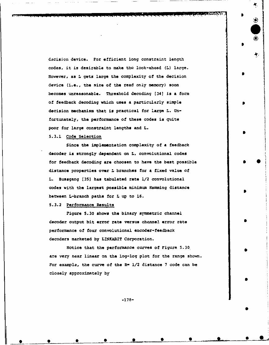
#1
30®
I
dacisicn device. For efficient long constraint length
codes, it is desirable to make the look-ahead (L) large.
However, as L gets large the complexity of the decision
device (i.e., the size of the read only memory) soon
becomes unreasonable. Threshold decoding (34] is a form
of feedback decoding which uses a particularly simple
decision mechanism that is practical for large L. Un-
fortunately, the performance of these codes is quite
poor for large constraint lengths and L.
5.3.1 Code Selection
Since the implementation complexity of a feedback
decoder is strongly dependent on L, convolutional codes
for feedback decoding are choosen to have the best possible S 0distance properties over L branches for a fixed value of
L. Bussgang [351 has tabulated rate 1/2 convolutional
codes with the largest possible minimum Hamming distance
between L-branch paths for L up to 16.
5.3.2 Performance Results
7igure 5.30 shows the binary symmetric channel
decoder output bit error rate versus channel error rate 5
performance of four convolutional encoder-feedback
decoders marketed by LINKABIT Corporation.
Notice that the performance curves of Figure 5.30.
are very near linear on the log-log plot for the range shown.
For example, the curve of the R- 1/2 distance 7 code can be
closely approximately by
-178-
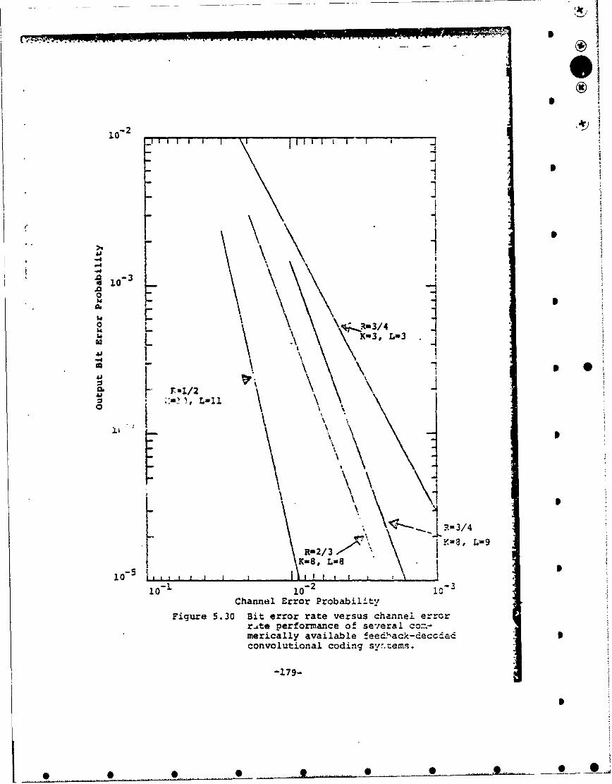
/
O
0- 2.I I I
j
-11
-3•
tjF--1
0
-, - 3 "L\-01
i0"• O"2 i-3/
1 . 0 -s -8, L=8
110-2
Channel Error Probability
Figure 5.30 Bit error rate versus channel errorrAte performance of se-:eral co..-merically available feedYack-decodedconvolutional coding syr.cems.
-179-
I
S • . . . . . . o _ 0 .. . . 0 _ _ 0,

4*
Pb '2000 p4 (5.29)
Figure 5.31 gives the 375-bit message error prob-
ability versus channel error rate performarce of the LINKABIT
R- 1/2 distance 7 code. As expected, since the output
errors tend to occur in bursts, Figure 5. 31 3hows that
the M-bit message error probability bound of MPb is •
somewhat pessimistic.
5.3.3 Implementation and Application Considerations
One advantage of feedback-decoded convolutional
coding is that interleaving/deinterleaving can be easily
implemented within the encoder/decoder. N-level inter-
leaving can be implemented by inserting N-bit shift
registers between every pair of register stages in the 5
encoder and in the syndrome generator of the decoder.
Then the decoder actually decodes N data streams inde-
pendently. This internal interleaving feature makes
feedback decoding attractive for burst error channels such
as the HP, troposcatter, and some telephone channels.
As with any rate b/v convolutional code, there
exists at the decoder a v-way ambiguity for serial input
sequences (i.e., node synchronization is required). This
ambiguity can be resolved by observing the rate at which
the decoder makes corrections and changing the synchro- S
nization position if too many errors seem to be occurring.
The encoder/decoders with node synchronization and
256-way internal interleaving/deinterleaving for the codes
S

"".I I I I
10-
10
-2%-
u 10 1
• ° I
• o..
Channel Error Probability
Figure 5.31 Message error probability Jversus channel error rate fora K-10, L-11, R-1/2-feedback-decoded convolutional codingsystem.
-1.1- .. . • I I Ir
i-.'
0•B
""_*"_ ' * _ __ __ _

of Figure 5.30 have all been implemented with less than 40
TTL integrated circuit chips.p
* .1
I
p
S _ __ 00 __ ____

6.0 Nonbinary Modulation Convolutional Codes
While Section 5 was concerned with binary con-
volutional codes, nonbinary convolutional codes can easily
be defined by replacing the binary symbols and modulo-2
arithmetic by symbols and arithmetic over a nonbinary
finite field. Such nonbinary coding systems are especially
useful with nonbinary modulation systems in which the mod-
ulation symbols are matched to the code symbols. For
example, a system with 2-ary orthogonal signal modulation
is ideally suited to a coding system with 2k-ary symbols.
One class of nonbinary convolutional codes which
has proved effective in obtaining small error rates on
channels with fading and non-Gaussian interference is that
of Viterbi-decoded dual-k convolutional codes. These codes
operate with 2k-ary symbols and are for channels with 2 k-ary
orthogonal signal modulation (e.g., MFSK).
Figure 6.1 shows the encoder for a R - 1/2, dual-3
code which has been implemented. The encoder shifts in one
k-bit (kM3 here) information symbol at a time and for each
k-bit input, two 2 -ary output symbols are generated. Each
2 k-ary output is used to select an orthogonal modulator
signal. A rate i/v encoder would, in general, use different
linear combinations of the present and past information sym-
bols to produce v, 2 k-ary outputs. Fiqure 6.2 shows a general
2 k-element finite field representation of a rate l/v, dual-k
convolutional encoder.
0 0 •• .wq. 0

K..° "'"" • ••FirstS• Output
iModu1e'-2 Addition rts(j
Figure 6.1 Rate 1/2, dual-3 convolutional encoder.
-1.8
Io-
bI
".•"I
&-°84
.5 ."•
,"% !
9 . 0.°0

OF (2) register stages
F g10 1F (2
942
w 1 2 -
0*
h'.L.
~k(j}c GF (2 )
Figure 6.2 Finite field representation of a rate ll/vdual-k convolutional encoder.
.- ..
%-.
,,.. , :~~. ! -~

S
* The demodulator consists of 2filters matched to
the0 orthogonal signals. So for each channel symbol,
quantized demodulator outputs are generated.
The Viterbi decoder for these codes must make 2
2 -way comparisons every v channel symbols. That is, after
each new branch of data is received the decoder comparesk*Uthe metrics of the 2paths entering each node (state)
kand eliminates all but the best. These 2 -way comparisons
are more difficult to implement than the binary comparisons
of rate 1/v codes, but for moderate values of kc reasonable
* implementations are possible. For example, a R - 1/2, dual-3
encoder/decoder with node synchronization and capable ofAoperating at i'formation bit rates of up to 100 Kbps has
* 0
been implemented by LINKABIT Corporation with about SO stand-
ard TTL integrated circuit chips. These codes have also
"I,"." ..
been implemented in software with a microprocessor.
The error rate performance of these codes can be
.. 2-,
determined using the simulation or analysis techniques des-
NIcribd in Sections S.1.9 and 5.1.10. The basic simulation
79 procedure is a straightforward modification of the binary
codes are usually used on channels with fading and non-Gaus-
S sian interference which are harder to model than the additi.ve
It ahite Gaussian noise channel commonly used with binary codes.
wh The transfer function error rate analysis technique
0o -1r6-
%>'-
*> 0 noedcdrwt noe 0nh nzain n 0aal of0

:,,. ® .n rr.- .t-'sr .. - u - ~-
for this class of codes is simplified by the fact that
the code transfer function for the codes in this class
with the best distance properties has been determined in
~ a closed form [37, 381. For a R - 1/v dual-k code the
"result is
T (INL T ( 2 1 ) D2 2Dv 61
In this nonbinary case the distance between two code
words is the numker of symbols in which the code words
I are different and the powers of D and N refer to the number
"of channel and infQrmation symbol, rather than bit, errors.
As in Section 5.1.10 let
N i.i-2v
r. - re.( kv)DV 2k V D
( 1 (6.2)
B Then the bit error probability can be upper bounded by
2k-1"' ~Pb a. Pi 6
21 i-2v
where P. is the probability of an error in comparint two
k-i ksequences which differ in i symbols. The 2 /(2 -1)
factor converts the k-bit symbol error probability to bit
-137-
* .. .. . . _ . . . . O .. . . . 9 . .. . . .. 0 .. . . . . 0 . . •0... .. . . ..

T~o ilutat h application of this bounding
technique for dual-k codes, consider a R - 1/2, dual-3
code with 8-ary orthogonal signal modulation (MFSX) and
noncoherent (square-law) demodulation on an independent
Rayleigh fading channel with no quant~ization. Then from
I Section 3.2.3
.- +J (1 '( .
oi -
where
p1-2u k (6) o
Using (6.4) for tho first two terms of (6.3) and the
bound [38]
P 1_< p4 (1-p)] + > 6 (6.6)I52I1-2p1 L '
for higher order terms (i !. 6) yields the results of
Figure 6.3. Figure 6.3 also shows the uncoded bound of
(3.11) for L-2 and 4 way diversity.
Comparing the curves in Figure 6.3 it can be seen
that the coded system is much better than the uncoded L-2
system with the same number of channel symbols per informationst
S~symbol and about 3 dB better than the uncoded L=4 system
"* __ 0-

L 3
S.L Order of Diversity -
Unccded L-22 Channel Symbols/
S L Information Symbol 0
-44
N- Uncoded L-4-W\ 4 Channel Symbols/V- Information Symbol 0
.0
OA
°
2R-1/2 Dual-310o6 2 Chnel, Symols/\\ __SfI.nformation Symbol
12 4 16 18 20 22 24 2,3
rb/No in dB 0
Figure 6.3 Performance of a R-i/2, dual-3 convolutionalcoding system with noncoherently demodulated8-ary MFSK on an independent Rayleigh fadingchannel with no quantization.
1
i .i139°
Se . . ..... • .. .• . ...... • . .... .• ,.. . _ • . . . .. .. .. ,, . ._ _O_

1
which has twice as many channel symbols per information
Symbol.
i I
* I
-190-
• • • S -- ... .. • I

7.0 Concatenated Codes IConcatenated coding is a technique which uses
two levels of coding as shown in Figure 7.1. Typically,
the inner code, i.e., the code that interfaces with
the channel, corrects most of the channel errors and
then a higher rate (lower redmudancy) outsr code reduces
the error rate to the desired level. The purpose of
concatenated coding is either to obtain a small error
rate with an overall encoder/decoder implementation com-
plexi-y which is less than that which would be required
by a single coding operation or to improve the error rate
performance of an existing coding system. Figure 7.1
also shows interleaving between the coding operations. * *This is usually required to breakup the error bursts out
of the inner coding operation.
7.1 Viterbi-Decoded Convolutional Inner Code and Reed-
Solo---t 01t.- M"
One of the most successful concatenated coding
systems is a system with a Viterbi-decoded conrolutional
inner code and a Reed-Solomon outer code with interleaving
(24,39,401. The Viterbi decoder in such a system takes
maximum advantage of soft quantized demodulator outputs to
improve the channel seen by the outer code by as much asp
possible. The outer code ~sees a channel, sometimes called
I
-121-
I
0 0 S 0_______

* .* .*�q�I S
Ii Io48
C1 48
S
6U
* p.Id 0*
4,Ido 4'U 0
C S- Ii
0UC
0� 05' U2 0
I.. 0'4 5 0
*4* 0- -414U V48
GFill -4 ci S-4L4J L�J-4
'4 00
Id '4U Ide* U'- .45'*48 0C
I
'I*
48
�1 O'��
S
0 S 0 __ 0 0

0
"- a superchannel, consisting of the inner encoder, the
true -.hannel, and the inner decoder which presents hard
quantized bursty data with a bit error rate typically
around 10" 2 . While an outer convolutional code could be
used, the bursty nature of the errors, the fact that only
hard quantized data is available, and the desirability of
a high rate code make a Reed-Solomon code, whose symbols
are formed from m-bit segments of the binary stream, a good
choice for the outer code. Since the performance of a Reed-
Solomon code only depends on the number of symbol errors in
the block, such a code is undisturbed by burst errors within
a it-bit symbol. But the concatenated system performance is
severely degraded by highly correlated errors among several
successive symbols. Hence the need for symbol (not bit)
interleaving between coding operations.
The performance of this concatenated coding system
can be determined by measuring the symbol error probability
out of the Viterbi decoder by simulation and then, assuming
the interleaving makes the symbol errors independent of each
other, using binomial type expressions to determine the
overall error probability. For example, given the symbol
error probability, p , versus inner code Eb/No for the inner
coding system alone, the overall symbol error probability
versus total Eb/No can be determined from (4.3) with
-193-
I

otal - nner _) (7.1)Router
where Router is the outer code rate. The bit error prob-
ability can be upper bounded by the symbol error prob-
ability (i.e., by assuming that any symbol in error has
all the bits in that symbol in error). If in addition, the 0
Bi of (4.3) are upper bounded by (4.4), then the total bit
error probability for the concatencated coding system ,ith
an m-bit per symbol Reed-Solomon outer code is bounded byI
i 2m1lk
2b < k-+ " ) (7.2)kZE+l 2m--
where E is the number of symbol errors the Reed-Solomon
decoder is capable of correcting and 2m-1 is the Reed-Solomon
symbol block length. The total code rate is the rate of the
inner code times the (2 -l-2E)/(2 -1) rate of the outer Reed-
Solomon code.
Figure 7.2 shows the bit errqr probability bound of
(7.2) versus I/No performance of this concatenated coding
system with a K-7, R-1/2 inner code and an m-8 bit/symbol
Reed-Solomon (R-S) outer code with various error correcting
capabilities. Additive white Gaussian noise and BPSK or QPSK
modulation are assumed. These curves show that for any error
rate there is an optimum number of errors that the R-S de-
coder should be designed to correct. This results
--I CIA
-A-Ai
• • •. • •aD• •

-gj
>1
0 .. . . .Nu be of. .... ..
.0 errors that theR-S decoder is ca-
1O~ pable of correctin~g.
Li
'A
10*
2.0 2.5 2.6 2.7 2.8 2.9 3.0 3.1.
in dBFigure 7.2 Concatenated code bit error probability perform~ance
with a K=7, R-1/2 convolutional inner code and an8-bit/sYmbol R-S outer code.
S ____ *eof ore•.tn
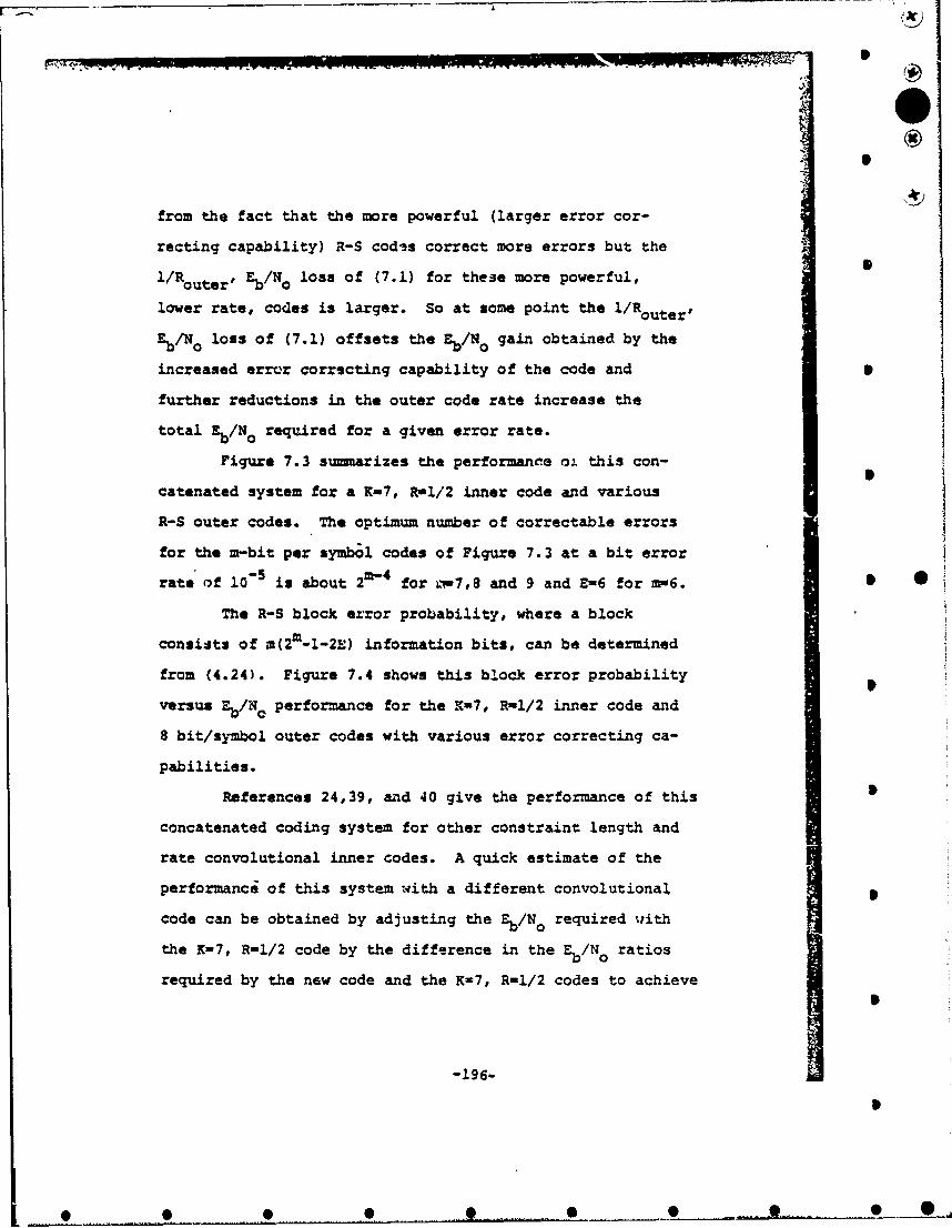
from the fact that the more powerful (larger error cor-
recting capability) R-S codss correct more errors but the
'/Router' E./NO loss of (7.1) for these more powerful,
lower rate, codes is larger. So at some point the l/Router,
b/No loss of (7.1) offsets the Eb/NO gain obtained by the
increased error correcting capability of the code and 9
further reductions in the outer code rate increase the
total Eb/No required for a given error rate.
Figure 7.3 summarizes the performance at this con-
catenated system for a K-7, R=1/2 inner code and various
R-S outer codes. The optimum number of correctable errors
for the m-bit per symbol codas of Figure 7.3 at a bit error
rate of 10- is about 2 for Lw7,8 and 9 and E-6 for m=6. S 0The R-S block error probability, where a block
consists of m(2m-l-2E) information bits, can be determined
from (4.24). Figure 7.4 shows this block error probability
versus E/Nc performance for the X-7, R-1/2 inner code and
8 bit/symbol outer codes with various error correcting ca-
pabilities.
References 24,39, and 40 give the performance of this 5
concatenated coding system for other constraint length and
rate convolutional inner codes. A quick estimate of the
performance of this system with a different convolutional
code can be obtained by adjusting the Eb/No required with
the K-7, R-1/2 code by the difference in the Eb/No ratios
required by the new code and the K-7, R-1/2 codes to achieve
1
-196-
S
S 5. 0-00 _• 0.

-"- " " - w - w ®
--
E- Number of symbolerrors that the R-Sdeioder is capableof correcting.
10"
>4
-4
Jka-s Symbol7 Utt Per zoo
*-I Symbol.Z41-4
2 1it. Pe2. .4
cod ands vaiusR oue1cds
m-,SydOJ10 Symb.....
-" •a~1-b"•k"
2.4 2.6 2.8 3.0 3.2 3.4 3.6 3t'
b/oin dB a
Figure 7.3 •uzmmary of concatenated coding b~t error p-.obab~.lity iiperformance with a K=7, R=l/2 convolutional. l.nercode and various R-S outer codes.
I]
S S S0 ~ 0* .Ii
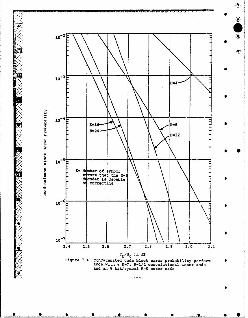
_ _ _ _ __
E-4
NS
"-24--
00
0 -
"1. E-24
10
£6610.
- 10-7
-2'.4 2 . 2 .2. . . . .
e rsthaitheaK-7,R12cnouinlinrcd
"co er is"ap bl
io6 -
"'- in dBn/i•.•ype~ •m.
and an 8 bit/symbol a-S outer code
IAM
• • • •• • ... ,, • • ,

A
some small inner code, nonconcaienated, error rntd,,r -2• . ~say Pb " 10"2
"The implementation and synchronization of tnis
concatenated coding system are discussed in (S9ý401. Re-
"ference 40 also investigates the sensitivity of this system
to nonideal receiver operating conditions such as pha e
and AGC errors and shows that it is not overly sensitive
"to these nonideal operating conditions. In [393 it is
estimated that a system with an mwS, E-l( R-S encoder/decoder
an inter!eae-er/4einterleaver suitable for operation with a
K-7, Ral/2 couvoltitional inner .-ode, And a block synchronizer
.! •all capable of operating at up to 100 Kbps could be imple-
ment*d with a total of about 220 integrated circuit chips.
-" 7.2 Viterbi-Decoded Convolutional Inner Code and Feedback-
Decoded Convolutional Outer Code
Another concatenated coding system which achieves a
more modest coding gain is a system with a Viterbi-decoded
convolutional inner code and a feedback-decoded convolutional
outer code with internal interleaving/deinterleaving. The
nice feature of this system is that the interleaving and de-
coding are simple to implemer.Figure 7.5 shows the bit error probability performance
of such a system with a K-7, R-1/3 inner code and the K-8,
V.h R-3/4, distance 5 code of Figure 5.30 as the outer code.
" This figure also shows the performance of the K-7, R-1/3 code
-199-
• O •• ,, . • O •• O

V ... . .
.0"5
.'K ; . ... : . •.....
"""-K-7, RI•-/3 Convolutional
10-6 Coding System
Concatenated Coding SystemSo4 with a K-7, R-l/3 Viterbi-Sdecoded Convolutional inner
"7, Code and a K-S, Rn3/4 Con-0A 0 volutional Outer Code
A.
5.4
l0NI3
4 5 6 7
EbNinne cde a 6
Figure 7.5- Performance of a concatenatedcoding system
Viterbi-decoded convolutionalinnercodeand a Kin8, .R-3/4
convolutional outer code.
r .20
"I i°'i°
-'. -200-
.. " ••o •
_ ; 0 . *'.. •

by itself. This concatenated coding system is seen to
improve the bit error rate versus Eb/NX performance of
the inner code when the bit error rate is less than about
105
• I
1201
-. O
L..-
P..
P*. p
I -01
. __00
-' W". T- 77
Appendix A. Glossary of Coding Terminoloy
1. Addition Modulo-2
Addition defined for a field with two elements(0 and 1) where 0+0 -0, 0+1 - 1, 1+0 - 1, and1+1 - 0. Somnetimzs denoted by 0.
2. AWGN
Additive White Gaussian Noise. Noise with a Gaussian.U Zplitude-proba~ility distribution and a constant
. power spectral density for all frequency ranges.- which is added to the received signal. In practice
as long as the noise power spectral density isconstant over the passband of the system, it isconsidered to be white noise. If the power spectral pdensity of the noise is not constant, the noise iscalled colored noise.
3. AGC
Automatic Gain Control.
4. Alphabet
The set of all possible distinct symbols that asource can generate.
Automatic Repeat Request. A feature which allowsfor requesting the retransmission of blocks, segments,or packets of data in which errors ray have been de-tected.
6. Bandwidth Expansion
The ratio of the bandwidth required by a system"relative to the bandwidth of some reference system.With coding the bandwidth expansion relative to an"uncoded system with the same modulation is the inverseof the code rate.
7. Binary CodeV..
A code in which the code symbols are from an alphabat-with two symbols.
k7.
-202-
.•

"8. Bit
A binary digit and a unit of information in,. ,Cinformation theory.9.• BSC
Binary Symetric Channel. A binary input and binary.output channel in-which the probability of an erroris constant independent of the transmitted symbol.
10. BPSK
Binary Phase-Shift Keying. A type of modulation ingnich t;wo phaies (usually 00 and 1800) are used toconvey information.
11. QPSK
Quaternary Phase-Shift Keying. A type of modulation1 In which four phases are used to convey information.
.. 12. PSK
.1 Phase-Shift Keying. A modulation technique that usesphase shifts-of a carrier to convey information.
a13. FSK
Frequency-Shift Keying. A modulation technique thatuses frequency shifts of a carrier to convey infor-
P imaticn.
14. Block Code
A code in which blockA of information or datasymbols uniquely specify blocks of encoded symbols.An (n,k) block code refers to a code with n codesymbols for every k information symbols.
15. Branch
In a convolutional code, the set of coded symbolsgenerated for a set of information or data symbols.For a rate R- b/v code a branch has v symbols. Abranch also describes the transitions for each setof data symbols in the tree, trellis, and statediagram representations of a convolutional code.
16. Bursts of Errors
In general terms, a sequence of data symbols witha higher than average error rate.
-203-
0 0 0 0_~9!

e" 1,911C T CITZZ'IL I"T
* 17. Channel
The media over which data are transmitted. Withcoding the channel can be viewed as a device that"transforms the encoded symbols at the transmitting"station into the decoder inputs at the receivingstation.
18. Encoder
A device that maps information or data symbolsinto coded symbols.
19. Decoder
A device that attempts to recover the transmittingstation information or data symbols from noisy
* receiving station data.
20. Channel Capacity (C)
The maximum rate at which information can be trans-mitted over a channel (in bits per binary channelsymbol) with an arbitrarily small probability oferror. •
21. Computational Cutoff Rate (RM)
With arbitrarily large constraint length sequential-decoded convolutional codes, the maximum rate forwhich the average amount of computation required todecode one bit of data is finite. Also a good limiton the rate of practical coding systems.
22. Code Rate (R)
The ratio of the number of information symbols to
the number of encoded symbols.
23. Codeword
An encoded sequence or block of symbols.
24. Codeword Weight
The number of nonzero symbols in a codeword.
25. Coherent Detection
A demodulation technique that requires knowledge ofthe phase and frequency of the received signal.
-204-
* * ~ *
i 0lS
26. Con-traint Length (K)
With convolutional codes, the total number ofbinary register stages in the encoder.
27. Convolutional Code 0
A coding technique in which the encoded sequenceis the convolution of the information sequenceand the code impulse response.
28. Free Dist&nce (df) •
r For a convolutional code, the minimum number ofencoded symbols in which any two arbitrarilylong encoded sequences differ.
29. Code Distance (d)
For block codes, the minimum number of symbolsin which any two codewords differ.
30. Diversity.
A technique in which two or more independentrealizations of a signal are obtained. It is used 0to combat fading and non-Gaussian interference.
31. Eb
Received energy per information bit.
32. S
Ratio of information bit energy to white noisesingle-sided (positive frequence only) powerspectral density.
33. FEC
Forward Error Correcting. A type of coding whereZhe decoder obtains an estimate of the informationsequence without the aid of a feedback channel.
34. Generator Matrix (G)
A matrix mapping of information symbols into encoded 0symbols in which the codewords are linear combinationsof the rows of the matrix.
35. Golay Code
A (23,12) block code with a code distance of 7.
-205-
. .......

(AD
36. Extended Golay Code
A (24,12) block code with a code distance of 8.
37. lazmming Codes
- m -
A class of single-error-correcting (2 m-1 , 2m-l-m)block codes.
38. Interleaving
The technique ol scrambling or changing the timesequence of codeword symbols. 5
39. Metric.
A goodness measure used in decoding algorit.hms.
40. Modem
Modulator and Demodulator41. Node.
For convoiutional codes, the junction of branchesin the tree or trellis representations. * •
42. Moncoherent Demodulation
A type of demodulation in which knowledge of thecarrier phase is not required.
43. Orthogonal Signals 0
Two signals s (t) and si(t) of duration T aredefined as or&ogonal i T~S i•jTS(t) sl(t) dt -0.
44. Soft QuantizationI
A technique of quantizing a demodulator output, definedover a continuum, such that in addition to a decisionas to which symbol was transmitted some quality infor-mation concerning the confidence we have in that de-cision is also provided.
45. Systematic Code 0A code in which the information symbols appear in thecodeword or encoded sequence in unaltered form.
46. Transparent CodeA code for which the complement of any codeword is
-
-206-

also a codeword. ;*
47. Tree Diagram
A representation of convolutional codes, usefulwith sequential or feedback decoding.
48. Trellis Diagram
A representatior of convolutional codes usefulwith Viterbi decoding.
49. Viterbi Decoding
A maximum-likelihood decoding tecrhniaue used for shortconstraint length convolutional codes.
50. Reed-Solomon CR-S) Codes
A class of (2m-l, 2m-l-2) E-erroi-correctingblock codes with symbolz from a 2 -ary alphabet.
51. DCI
Bose, _Chaudhuri, and Hodquengham Codes. A class3f blo~k codes with well-defined algebraic decoding | *algorithms.
52. Concatenated Coding
A technique of coding which uses more than one levelof coding. For eramle, with two levels of codingthe inner encoder and decoder operate over the truechannel while the outer encoder and decoder operateover a channel consisting of the inner encoder, thetrue channel and the inner decoder.
53. Catastrophic Error Propagation.
With cenvolutional codes, the oracerty of some codesthat with an arbitrarily lonc c.2!ýca sequence a finitenumber of channel errors can cause an arbitxaril,large number of decoded bit errors. This con-dition can be avoided by proper code selection.
54. Secuential Decoding
A decoding technique for convolutional codes whichinvolves searching through the code tree represen-tation. The search or computation time is a randomvariable depending on the noise statistics.
-207-
O . .... .......... .. . . . ••'• • ,,....... . •• S
0• _ . .. . . .. . . .. .. . .... . .

55. Feedback Decoding
A decoding technique for convolutional codes inwhich decoding decisions at any given time affectdecisions in the future. No feedback channelis used.
56. Differentially Coherent
A type of demodulation ia which the reference signalfor demodulation is derived from the receiver inputover the previous input symbol.
57. DBPSK or DPSK
Differentially Coherent Binary Phase-Shift Keying.
sq. DQPS
Differentially Coherent uatoernary Phase-Shiftleying.
* .
*

O
APPENDIX B. GLOSSARY OF SYMBOLS
C Channel capacity
d Code distance
df Free distance
Eb/NO Information bit energy-to-noise ratio
E INO Channel symbol energy-to-noise ratio
G Generator matrix of a linear block code
K Convolutional code constraint length
L Order of diversity or look-ahead distance of
a feedback-decoded convolutional decoder.
R Code rate •
RO Computational cutoff rate
0 Modulo-2 addition
2
,*
II
*

0*®
REFERENCES
1. A. J. Viterbi, Principles of Coherent CommunicationNew York: McGraw-Hill, 1966.
2. S. W. Golomb (ed.), Digital Communications with SpaceAeplications. Englewood Clilfts, N.J: Prentice-Hall,
3. C. E. Shannon, 'A Mathematical Theory of Communic.2tion,"Bell System Technical Journal, Vol. 27, pp. 379-423,1948.
4. J. 4 Wozencraft and I. M. Jacobs, Principles of Commu-nication Engineering. New York: Wiley, 1965.
5. R. G. Gallager, Information Th-.ary and Reliable Commu-nication. New York: Wiley, 1968.
6. L. E. Miller and J. S. Lee, "Th Probability DensityFunction for the Output of an Analog Cross-Correlatorwith Correlated Bandpass Inputs," IEEE Trans. Inform.Theory, Vol. IT-20, pp. 433-440, July 1974. * .•
7. A. Kohlenberg and G. D. Forney, Jr., "ConvolutionalCoding for Channels with Memory," IEEE Trans. Inform.Theory, Vol. IT-14, pp. 618-626, September 1963.
8. 1. Y. Tong, "Burst-Trapping Techniques for a CompoundChannel," IEEE Trans. Inform. Theory, Vol. IT-15, pp.710-715, November 1969.
9. S. Y. Tong, "Performance of Burst-Trapping Codes,"Bell System Tech. J., Vol. 49, pp. 477-491, April1970.
10. H. 0. Burton, D.D. Sullivan, and S. Y. Tong, *GeneralizedBurst-Trapping Codes," IEEE Trans. Inform. Theory,Vol. IT-17, pp. 736-742, November 1971.
11. D. Chase, wA Class of Algorithms for Decoding BlockCodes with Channel Measurement Information, "IEEETrans. Inform. Theory, Vol. IT-18, pp. 170-182,7Janua ry r97§
12. "Troposcatter Interleaver Study Report," CNR, Inc.,Report Number RADC-TR-75-19 for Rome Air Dev. Center,Air Force Systems Command, Griffiss AFB, N.Y.,February 1975.
I
I'I9 9

(D
13. S. K. Leung-..au:-Cheong and M.E. Hellman, "Concerninga Bound on Undetected Error Probability,* IEEE Trans.Inform. Theory, Vol. IT-22, pp. 235-237, Mirch 1976.
14. W. W. Peterson, Error Correcting Codes. Cambridge,Mass.: MIT Press, -191.
15. E. R. Berlekamp, Algebraic Coding Theory. New York:ifcGraw-Hill, 1968.
16. G. D. Forney, Concatenated Codes. Cambridge, Mass.:MIT Press, 1966.
17. C. C-ihn, "Performance of a Digital Phase ModulationComi.unications Sys'ý-em," Ramo-Wooldridge Reportt4i/0-905, April 1951.
18. R. W. Moss and R. D. Wetherington, "Sensitivity Analysi3of Link Transmissions Study," Vol. 1, Georgia instituteOf Tech., Eng. Experiment Station Report prepared forElectronics Systems Division, Air Force Systems Com-mand, Belford, Mass. under Contract F19628-74-C-0180,December 1974.
19. A. J. Viterbi and I. M. Jacobs, "Advancea in Codingand Modulation for Noncoherent Channels Affected byFading, Partial Band, and Multiple-Access Interference,"in Advances in Communication Systems, Vol. 4, A. J.Viterbi, Ed. Nett York: Academic Press, pp. 279-308,1975.
20. A. J. Viterbi, "Error Bounds for Convolutional Codesand an Asymptotically Optimum Decoding Algorithm,*IEEE Trans. Inform. Theory, Vol. IT-13, pp. 260-269,"April 1967.
21. L. Lee, "Concatenated Coding Syetems Employing Unit-Memory Convolutional Codes and Symbol-Oriented OptimalDecoding Algorithms," Ph. D. dissertation, University 0of Notre Dame, Notre Dame, Indiana, May 1976.
22. J. L. Massey end M. K. Sain, "Inverses of LinearSequential Circuits, "IEBE Trans. Computers, Vol. C-17,pp. 330-337, Apcil 1968.
23. W. J. Rosenberg, "Structural Properties of Convolutional 0Codes," Ph. 'issertation, School Eng. and Appl.Science, Uni,- k: ity of California, Los Angeles, 1971.
24. J. P. Odenwalder, "Optimal Decoding of Convolutional Codes,"
2
-211-
S

0
Ph.* D. dissertation, School Eng. and Appi. Science,University of California, Los Angeles, 1970.
25. K. G. Larsen, *Short Convolutional ---odes with MaximalFree Di.stance for Rate 1/2, 1/3 and 1/4,0 IEEE Trans.Inform. Theory, Vol. !T-19, pp. 371-372, May 193. ~ 0
26. E. Paasko, *Short Binary Convolutional Codes withJ ~~Maximal Pree Distance for Rates 2/3 and 3/4,"IETrans. Inform. heo , Vol. IT-2O, pp. 683-689',September1974.
27. -). A...Hller and 1. M. Jacobs, "Viterbi-Decoding forSatellite and Space Communication," IZEE Trans.Commun. Technol., Vol. COH-19, pp.835-847, October 1971.
28. A.'J. Vitembi, wCon~volutiona3. Codes and Their Per-Formance in Communication Systes, " IEEE Trans.Commun. Technol., Vol. COM.19, pp. 751772, Otober 1971.
29. A. J. Viterbi, "Convolutional Codes and Their Per-formance in Communication Systems," LINKABIT Corp-oration, San Diego, Calif., Seminar Notes, 1970.
30. G. 0. Forney, Jr., "Tise of a Sequential Decoderto Analyze Convolutional Code Structure,* IEEE Trans.*Inform. Theory, Vol. IT-16, pp. 793-795, November 1970.0
.°
:4 31. R. Johannesson, e Robustly Optimal Rate One-SialfBinary C.nvolutional Codes," IEEE Trans. Inform.Theory, Vol. IT-21, pp. 464-468, July 1975.
32. J. L. Massey and 0. J. Costello, Jr., *NonsystematicConvolutional Codes for Sequential Decoding in SpaceApplications," IEEE Trans. CoTmun. Technol., Vol.COM-19, pp. 806-813, October 1971.
33. J. A. Hoeller, "Fedback Decoding of ConvolutionalCodes," in Advances in Communication Systems, Vol. 4,A. J. ViteAci, Edoneo rkn cademic Press, pp. 2e1-278, 1975.
34. J. L. Massey, Threshold Decodin . Cambridge, Mass.:
FIT Press, 1;63.~
35 J. J. Bussgang, "Some Properties of Binary Convolutional"Code Generators," IEEE Trans. Inform. Theory, Vol.IT-ho, pp. 90-100, January 1965.
-212-
32. . .asean .. otl, .,Nosys9ea.j

S'., •
w A
36. wStudy of Information Trans for Optimizatio~a toz'Communication SatelI ites," LINKABIT Corporation,"San Diego, CaliforT, .a, Final Peport under ContractNAS2-6810 for NASA Ames Res. Center, Moffett FieldCalifornia, NASA Report CR 114561, January 1973.
37. "Verdin Mode Improvement Task,O LINKABIT Corporation,San Diego, California, Final Report for Navy ElectronicLab. Center, San Diego, California, (Confidential),April 1975.
I. 38. J. P. Odenwalder, 'Dual-k Convolutional Codes forNoncoherently Dozodulated Channels," to be published Sin Proceeding of the 1976 Int:rnational TelemeteringCon-., October 1976.
39. *Hybrid Ceding System Study," LINKABIT Corporation,San Diego, CAlifornia, Final Reporc under ContrrctNAS2-6722 for NASA Ames Res. Canter, Moffett Field,California., NASA Report CR 114486, September 1972.
- 40. wConcatenated Read-Solomon/Viterbi Channel Codingfor Advanced Planetary Missions: Analys.is, Simulations,and Test,* LnqKABIT Corporation, San Diego, California,"Final Report undre Contract 953866 for Jet PropulsionLab., Pasadena, California, December 1974. *
41. "*Zror Protection wAnual,u Computer Sciences Corporation,Falls ýhurch, Va., Report prepared for Rome Air Dev."Center, Air Force Systems Command, Griffiss AFB, N.Y.,1972.
%.p
S2'
:2'_
t"F -:13-
I