Embed Size (px)
Citation preview

39
BoundedQuery Rewriting Using Views
YANG CAO, University of Edinburgh
WENFEI FAN, University of Edinburgh and Beihang University
FLORIS GEERTS, University of Antwerp
PING LU∗, Beihang University
A query Q in a language L has a bounded rewriting using a set of L-definable views if there exists a query Q ′
in L such that given any dataset D,Q(D) can be computed byQ ′that accesses only cached views and a small
fraction DQ of D. We consider datasets D that satisfy a set of access constraints, which are a combination of
simple cardinality constraints and associated indices, such that the size |DQ | of DQ and the time to identify
DQ are independent of |D|, no matter how big D is.
In this paper we study the problem for deciding whether a query has a bounded rewriting given a setV
of views and a set A of access constraints. We establish the complexity of the problem for various query
languages L, from Σp3-complete for conjunctive queries (CQ), to undecidable for relational algebra (FO). We
show that the intractability for CQ is rather robust even for acyclic CQ with fixedV and A, and characterize
when the problem is in PTIME. To make practical use of bounded rewriting, we provide an effective syntax for
FO queries that have a bounded rewriting. The syntax characterizes a key subclass of such queries without
sacrificing the expressive power, and can be checked in PTIME. Finally, we investigate L1-to-L2 bounded
rewriting, when Q in L1 is allowed to be rewritten into a query Q ′in another language L2. We show that
this relaxation does not simplify the analysis of bounded query rewriting using views.
CCS Concepts: • Information systems→ Database query processing;
Additional Key Words and Phrases: Bounded rewriting; big data; complexity
ACM Reference format:Yang Cao, Wenfei Fan, Floris Geerts, and Ping Lu. 2017. Bounded Query Rewriting Using Views. ACM Trans.Datab. Syst. 9, 4, Article 39 (December 2017), 60 pages.
https://doi.org/0000001.0000001
1 INTRODUCTIONTo make query answering feasible in big datasets, practitioners have been studying scale indepen-
dence [5–7]. The idea is to compute the answers Q(D) to a query Q in a dataset D by accessing a
bounded amount of data in D, no matter how big the underlying D is.
This idea was formalized in [25, 26]. As suggested in [26], nontrivial queries can be scale
independent under a set A of access constraints, a form of cardinality constraints with associated
indices. A query Q is boundedly evaluable [25] if for all datasets D that satisfy A, Q(D) can be
computed from a fractionDQ ofD, and the time for identifying and fetchingDQ , and hence the size
∗Corresponding author
Permission to make digital or hard copies of all or part of this work for personal or classroom use is granted without fee
provided that copies are not made or distributed for profit or commercial advantage and that copies bear this notice and the
full citation on the first page. Copyrights for components of this work owned by others than the author(s) must be honored.
Abstracting with credit is permitted. To copy otherwise, or republish, to post on servers or to redistribute to lists, requires
prior specific permission and/or a fee. Request permissions from [email protected].
© 2017 Copyright held by the owner/author(s). Publication rights licensed to Association for Computing Machinery.
0362-5915/2017/12-ART39 $15.00
https://doi.org/0000001.0000001
ACM Transactions on Database Systems, Vol. 9, No. 4, Article 39. Publication date: December 2017.

39:2 Yang Cao, Wenfei Fan, Floris Geerts, and Ping Lu
|DQ | of DQ are independent of |D|. We identify DQ by reasoning about the cardinality constraints
in A, and fetch DQ by using the indices of A.
Bounded evaluation has proven useful [11, 14, 16]. Experimenting with several real-life datasets,
it was shown that under a couple of hundreds of access constraints, 77% of randomly generated
conjunctive queries (a.k.a. SPC queries) [16], 67% of relational algebra queries [11], and 60% of graph
pattern queries [14] are boundedly evaluable on average. Query plans for boundedly evaluable
queries outperform commercial query engines by 3 orders of magnitude, and the gap gets larger
on bigger data.
As an example of bounded evaluability, consider a Graph Search query of Facebook [23]: find meall restaurants in NYC which I have not been to, but in which my friends have dined in May 2015. Acardinality constraint imposed by Facebook is that a person can have at most 5000 friends [24].
Another one is that one dines at most once per day. Given these and another two similar constraints,
the query can be answered by accessing 470000 tuples [11], as opposed to billions of user tuples
and trillions of friend tuples in the Facebook dataset [31].
Still, many queries are not boundedly evaluable. Can we do better for such queries? An approach
that has proven effective by practitioners is by making use of views [7]. The idea is to select and
materialize a set V of small views, and answer Q on a dataset D by using views V(D) and an
additional small fraction of D. That is, we cache V(D) with fast access, and compute Q(D) by
using V(D) and by restricting costly I/O operations to (possibly big) D. Many real-life queries
that are not boundedly evaluable can be efficiently answered by using small views and by accessing
a bounded amount of additional data in D [7].
Example 1.1. Consider a Graph Search queryQ0: findmovies that were released by Universal Studiosin 2014, liked by people at NASA, and were rated 5. The query is defined over a relational schema R0
consisting of four relations: (a) person(pid, name, affiliation), (b)movie(mid,mname, studio, release),(c) rating(mid, rank) for ranks of movies, and (d) like(pid, id, type), indicating that person pid likes
item id of type, including but not limited to movies. Over R0, Q0 is written as a conjunctive query:
Q0(mid) = ∃xp ,x ′p ,ym
(person(xp ,x ′
p , “NASA”) ∧ movie(mid,ym , “Universal”, “2014”)
∧ like(xp ,mid, “movie”) ∧ rating(mid, “5”)).
Consider a setA0 of two access constraints: (a) φ1 = movie((studio, release)→ mid, N0), stating that
each studio releases at most N0 movies each year, where N0 is obtained by aggregating R0 instances;
an index is built on movie relation such that given any (studio, release) value, it returns (at most N0)
corresponding mids; we find that typically N0 ≤ 100 in practice; and (b) φ2 = rating(mid → rank,1), stating that each movie has a unique rating; an index is built on rating to fetch rank as above.
Under A0, query Q0 is not boundedly evaluable. Indeed, an instance D0 of R0 may have billions
of person and like tuples [31], and no constraints in A0 can help us identify a bounded fraction
of these tuples to answer Q0.
Nonetheless, suppose that we are given a view that collects movies liked by NASA folks, defined
as the following conjunctive query:
V1(mid) = ∃xp ,x ′p ,y
′m , z1, z2
(person(xp ,x ′
p , “NASA”) ∧ movie(mid,y ′m , z1, z2)
∧ like(xp ,mid, “movie”)).
As will be seen later, Q0 can be rewritten into a conjunctive query Qξ using V1, such that for all
instances D0 of R that satisfy A0, Q0(D0) can be computed by Qξ that accesses only V1(D0) and
an additional 2N0 tuples from D0, no matter how big D0 grows. Here V1(D0) is a small set, much
smaller than D0. □
ACM Transactions on Database Systems, Vol. 9, No. 4, Article 39. Publication date: December 2017.

BoundedQuery Rewriting Using Views 39:3
To support scale independence using views, practitioners have developed techniques for selecting
views, indexing the views for fast access and for incrementally maintaining the views [7]. However,
there are still fundamental issues that call for a full treatment. How should we characterize scale
independence using views? What is the complexity for deciding whether a query is scale indepen-
dent given a set of views and access constraints? If the complexity of the problem is high, is there
any systematic way that helps us make practical use of cached views for querying big data?
Contributions. This paper tackles these questions.
(1) Bounded rewriting. We formalize scale independence using views, referred to as bounded rewrit-ing (Section 2). Consider a query language L, a set V of L-definable views and a database schema
R. Informally, under a set A of access constraints, we say that a query Q ∈ L has a boundedrewriting Q ′
in the same L using V if for each instance D of R that satisfies A, there exists a
fraction DQ of D such that
• Q(D) = Q ′(DQ ,V(D)), and
• the time for identifying DQ and hence the size |DQ | of DQ are independent of |D|.
That is, we compute the exact answers Q(D) via Q ′by accessing cached V(D) and a bounded
fraction DQ of D. While V(D) may not be bounded, we can select small views following the
methods of [7], which are cached with fast access. We formalize the notion in terms of query plans
in a form of query trees commonly used in database systems [42], which have a bounded sizeMdetermined by our resources such as available processors and time.
(2) Complexity. We study the bounded rewriting problem (Section 3), referred to as VBRP(L) for a
query language L. Given a set A of access constraints, a query Q ∈ L and a set V of L-definable
views, all defined on the same database schema R, and a boundM , VBRP(L) is to decide whether
under A, Q has a bounded rewriting in L using V with a query plan of size no larger than M ,
referred to as anM-bounded query plan.The need for studying VBRP(L) is evident: if Q has a bounded rewriting, then we can find
efficient query plans to answer Q on possibly big datasets D. We investigate VBRP(L) when L
ranges over conjunctive queries (CQ , i.e., SPC), unions of conjunctive queries (UCQ , i.e., SPCU),positive FO queries (∃FO+, select-project-join-union queries) and first-order logic queries (FO, the
full relational algebra). We show that VBRP is Σp3-complete for CQ , UCQ and ∃FO+, but it becomes
undecidable for FO. In addition, we explore the impact of various parameters (R,M , A and V) of
VBRP on its complexity.
(3) Acyclic conjunctive queries. Worse still, we show that the intractability of VBRP is quite robust
(Section 4). It remains intractable for acyclic conjunctive queries (denoted by ACQ), when all
parametersM , R, A and V are fixed, and even when access constraints in the fixed A have quite
restricted forms. In light of this, we give a characterization for VBRP(ACQ) to be in PTIME, andidentify several sub-classes of ACQ and CQ for which VBRP is tractable under fixedM ,R,A andV .
(4) Effective syntax. To cope with the undecidability of VBRP(FO) and the robust intractability of
VBRP(CQ), we develop an effective syntax for FO queries that have a bounded rewriting (Section 5).
For any R,V,A and M , we show that there exists a class of FO queries, referred to as queriestopped by (R,V,A,M), such that under A,
(a) every FO query that has anM-bounded rewriting usingV is equivalent to a query topped
by (R,V,A,M);
(b) every query topped by (R,V,A,M) has anM-bounded rewriting in FO usingV that can
be identified in PTIME; and
ACM Transactions on Database Systems, Vol. 9, No. 4, Article 39. Publication date: December 2017.

39:4 Yang Cao, Wenfei Fan, Floris Geerts, and Ping Lu
(c) it takes PTIME inM, |Q |, |V|, |R |, |A| to check whether Q is topped by (R,V,A,M), using
an oracle to check whether views inV have bounded output (see below).
That is, topped queries make a key subclass of FO queries with a bounded rewriting using V ,
without sacrificing their expressive power, along the same lines as safe-range queries for safe
relational calculus (see, e.g., [1]). This allows us to reduce VBRP to syntactic checking of topped
queries. Given a query Q , we can check syntactically whether Q is topped by (R,V,A,M) in
PTIME, by condition (c) above; if so, we can find a bounded rewriting in PTIME as warranted by
condition (b); moreover, ifQ has a bounded rewriting, then it can be transformed to a topped query
by condition (a).
To check topped queries, we need to determine whether some views of V have bounded outputV(D) over all datasets D that satisfy A, i.e., the size |V(D)| is bounded by a constant. This is to
ensure bounded accesses to D, since a query plan may filter and fetch data from D by using values
from some views in V(D). This problem is, not surprisingly, undecidable for FO (Section 3). In
light of this, we develop an effective syntax for FO queries with bounded output. That is, given A
and R, we identify a class of FO queries, referred to as size-bounded queries, such that under A,
an FO view (query) over R has bounded output if and only if it is equivalent to a size-bounded
FO query, and it is in PTIME to check whether a query is size-bounded. We use this as a PTIMEoracle when checking topped queries (condition (c)) above.
Experimenting with CDR (call detail record) data and queries from one of our industry collabo-
rators, we find that bounded query rewriting using views improves more than 90% of their queries
from 25 times to 5 orders of magnitude [15].
(4) Rewriting in another language. Finally, we study L1-to-L2 bounded rewriting, when we are
allowed to rewrite a query Q ∈ L1 into a query Q ′in another query language L2 (Section 6).
We reinvestigate the bounded rewriting problem in this setting, denoted by VBRP+(L1,L2). It
is the problem for deciding, given a set A of access constraints, a query Q ∈ L1, a set V of
L1-definable views, and a bound M , whether under A, Q has a rewriting Q ′ ∈ L2 using V that
has anM-bounded query plan.
One might be tempted to think that this relaxation would make our lives easier. However,
we show that VBRP+ remains Σp3-hard for CQ-to-L2 when L2 ranges over UCQ , ∃FO+and FO;
similarly when L1 is UCQ or ∃FO+.This work is an effort to give a formal treatment of scale independence with views, an approach
that has been put in action by practitioners. The complexity bounds reveal the inherent difficulty
of the problem. The effective syntax, however, suggests a promising direction for making use
of bounded rewriting. Various techniques are used in the proofs, including characterizations,
algorithms and a wide range of reductions.
2 BOUNDED QUERY REWRITINGIn this section we formalize bounded query plans and bounded query rewriting using views under
access constraints. We start with a review of basic notions.
Database schema. A relational (database) schema R consists of a collection of relation schemas
(R1, . . . ,Rn), where each Ri has a fixed set of attributes. We assume a countably infinite domain U of
data values, on which instances D of R are defined. We use |D| to denote the size of D, measured
as the total number of tuples in D. Instances of a single relation schema R are denoted by D.
Access schema. Following [25], we define an access schema A over a database schema R as a
set of access constraints φ = R(X → Y ,N ), where R is a relation schema in R, X and Y are sets of
attributes of R, and N is a natural number.
ACM Transactions on Database Systems, Vol. 9, No. 4, Article 39. Publication date: December 2017.

BoundedQuery Rewriting Using Views 39:5
For an instance D of R and an X -value a in D, we denote by DR:Y (X = a) the set{t[Y ] | t ∈
D, t[X ] = a}, and write it as DY (X = a) when R is clear in the context. An instance D of R satisfies
access constraint φ if
• for any X -value a in D, |DR:Y (X = a)| ≤ N ; and
• there exists a function (referred to as an index) that given anX -value a, returns DR:XY (X = a)(i.e.,
{t[XY ] | t ∈ D, t[X ] = a
}) from D in O(N ) time.
Intuitively, an access constraint is a combination of a cardinality constraint and an index on X forY (i.e., the function). It tells us that given any X -value, there exist at most N distinct corresponding
Y -values, and theseY values can be efficiently fetched by using the index. For instance,A0 described
in Example 1.1 is an access schema.
Note that functional dependencies (FDs) are a special case R(X → Y , 1) of access constraints, i.e.,when bound N = 1, provided that an index is built from X to Y .
An instanceD of R = {R1, . . . ,Rn} satisfies access schemaA, denoted byD |= A, if the instance
of Ri in D satisfies all the access constraints φ = Ri (X → Y ,N ) in A.
Query classes. We express queries and views in the same language L.
Following [1], we consider atomic formulas that are either relation atoms R(x) for R ∈ R, or
equality atoms x = y or x = c , where x , x and y variables and c is a constant. We consider the
following classes L of queries built up from atomic formulas.
• Queries in first-order logic (FO) are inductively defined as follows: (a) atomic formulas are
FO queries, and (b) if Q , Q1 and Q2 are FO queries, then so are Q1 ∧Q2, Q1 ∨Q2, ¬Q , ∃x Qand ∀x Q (see Chapter 5 of [1] for details).
• Positive existential FO queries (∃FO+) are FO queries in which negation (¬) and universal
quantification (∀) are disallowed.• Conjunctive queries (CQ) are ∃FO+queries in which disjunction (∨) is disallowed. A CQquery can bewritten asQ(x) = ∃x ′ϕ(x , x ′), whereϕ(x , x ′) is a conjunction of atomic formulas
(see Chapter 4 of [1]).
• Unions of conjunctive queries (UCQ) are of the formQ(x) =Q1(x)∪ · · · ∪Qk (x), whereQi (x)is a CQ for i ∈ [1,k]. It is known that each ∃FO+query Q can be written as a UCQ , which
may possibly result in exponential increase in size |Q | [43].
Bounded query rewriting. To simplify the definition, we present bounded query rewriting in
terms of the relational algebra with projection π , selection σ , Cartesian product ×, union ∪, set
difference \ and renaming ρ. Consider an access schema A and a setV of views, both defined over
the same database schema R. We first extend the relational algebra under A withV , denoted by
RAA,V , as follows:
Q ::= c | fetch(X ∈ Q,R,Y ) | V | πY (Q) | σC (Q) | Q ×Q | Q ∪Q | Q \Q | ρx→yQ,
where c is a constant, x and y are variables, V is a view inV , πY (Q),σC (Q),Q ×Q,Q ∪Q , Q \Qand ρx→yQ denote projection, selection, Cartesian product, union, set difference and renaming
as in the relational algebra, respectively; fetch(X ∈ Q,R,Y ) requires that φ = R(X → Y ,N ) is an
access constraint in A and that Q(D) returns a set of X -attributes of R given an instance D of
R; for each a in Q(D), it retrieves DR:XY (X = a) in the instance D of R in D by using the index
associated with φ. Similarly, we also define LA,V for fragment L of RAA,V that corresponds to
CQ , UCQ or ∃FO+.Intuitively, RAA,V revises the relational algebra by replacing direct access to relation R with
fetch(X ∈ Q,R,Y ), i.e., it accesses instances of R only via the indices of access constraints in A
only. It also allows accesses to cached views of V .
ACM Transactions on Database Systems, Vol. 9, No. 4, Article 39. Publication date: December 2017.

39:6 Yang Cao, Wenfei Fan, Floris Geerts, and Ping Lu
Consider a query Q in a language L. For a natural numberM , we say that Q has anM-boundedrewriting in L usingV under A, or simply a bounded rewriting usingV whenM and A are clear
from the context, if there exists a query Q ′ ∈ LA,V such that (a) all constants in Q ′are taken from
Q , (b) for all instances D of R satisfying A, Q(D) = Q ′(D), and (c) there are at mostM constants
and operations (fetch,V ,π ,σ ,×,∪, \, ρ) in Q ′.
Intuitively, under A, query Q is equivalent to Q ′, i.e., Q ′
is a rewriting of Q using V . Moreover,
whileQ ′can retrieve entire cached views, its access to the underlyingD must be via fetch operations
only, by using the indices in the access constraints of A. Hence only a bounded amount of data is
fetched from D. HereM is a threshold picked by users and is determined by available resources.
The less resources we have, the smallerM we can afford. Without the boundM , we find that the
query Q ′is often of exponential length when experimenting with real-life data, which are not very
practical; indeed, it would be EXPSPACE-hard to decide whether there exists a bounded rewriting
even for CQ , by reduction from the problem for deciding bounded evaluability for CQ [25]. Hence
we opt to let users specifyM based on their resources.
We next give an “operational semantics” of rewritings, by means of query plans.
Query plans. Following [42], we define a query plan using V , denoted by ξ (V,R), as a tree Tξ that
satisfies the following two conditions.
(1) Each node u of Tξ is labeled Si = δi , where Si denotes a relation for partial results, and δi is asfollows:
(a) {c} for a constant c , if u is a leaf of Tξ ;(b) a view V for V ∈ V , if u is a leaf of Tξ ;(c) fetch(X ∈ S j ,R,Y ) if u has a single child v labeled with S j = δ j , and S j has attributes X ; Here
X and Y are attributes in R and X can possibly be empty;
(d) πY (S j ), σC (S j ) or ρ(S j ), ifu has a single childv labeled with S j = δ j ; hereY is a set of attributes
in S j , and C is a condition defined on S j ; or(e) S j × Sl , S j ∪ Sl or S j \ Sl , if u has two children v and v ′
labeled with S j = δ j and Sl = δl ,respectively.
Intuitively, given an instance D of R, relations Si ’s are computed by δi , bottom up inTξ [42]. More
specifically, δi may (a) extract constant values, (b) access cached views V (D), and (c) access D via
a fetch operation, which, for each a ∈ S j , retrieves DR:XY (X = a) from the instance D of R in D on
which the fetch operator is defined; it may also be a relational operation ((d) and (e) above).
(2) For each instance D of R, the result ξ (D) of applying ξ (V,R) to D is the relation Sn at root of
Tξ computed as above.
The size of plan ξ is the number of nodes inTξ . We use Dξ to denote the bag of all tuples fetched
for computing ξ (D), i.e., the multiset that collects tuples in DR:XY (X = a) for all fetch(X ∈ S j ,R,Y ).Intuitively, it measures the amount of I/O operations used to access D. Note that tuples retrieved
from the cached views do not incur any I/O.
Example 2.1. A plan ξ0(V1,R0) using view V1 is depicted in Fig. 1. Given an instance D of R0, (a)
it fetches the set S4 of mids of all movies released by Universal Studios in 2014; (b) filters S4 with
mids in V1(D) via join, to get a subset S8 of S4 of movies liked by NASA folks; (c) fetches ratingtuples using the mids of S8; and (d) finds the set S11 of mids. One can verify that ξ0(D) = Q0(D)
for Q0 given in Example 1.1. □
Bounded plans. Consider an access schema A over R. A query plan ξ (V,R) is said to conform toA if (a) for each fetch(X ∈ S j ,R,Y ) operation in ξ , there exists an access constraint R(X → Y ′,N )
ACM Transactions on Database Systems, Vol. 9, No. 4, Article 39. Publication date: December 2017.
BoundedQuery Rewriting Using Views 39:7
S11 = πmid(S10)
S10 = σrank=5(S9)
S9 = fetch(mid ∈ S8, rating, (mid, rank))
S8 = πmid(S7)
S7 = σS4 .mid=V1 .mid(S6)
S6 = S4 × S5
S4 = fetch((studio, release) ∈ S3,movie,mid)
S3 = S1 × S2
S1 = “Universal” S2 = “2014”
S5 = V1
Fig. 1. A query plan ξ0 using view V1.
in A such that Y ⊆ X ∪Y ′, and (b) there exists a constant Nξ such that for all instances D |= A of
R, |Dξ | ≤ Nξ .
That is, ξ can access cached views, and fetch Dξ from D controlled by access schema A. Plan ξtells us how to retrieve Dξ such that ξ (D) is computed by using the data in Dξ and V(D) only.
Better still, Dξ is bounded: |Dξ | is decided by Q and constants N in A only, and is independent of
possibly big |D|. The time for identifying and fetching Dξ is also independent of |D| (assuming
that given an X -value a, it takes O(N ) time to fetch DR:XY (X = a) from the instance D of R in D,
via the index for R(X → Y ,N )).
Given a natural number M , we say that ξ (V,R) is M-bounded for query Q using V under Aif (a) ξ conforms to A, (b) the size of ξ is at most M , (c) for all D |= A, Q(D) = ξ (D),i.e., Q is
equivalent to ξ on all instances D |= A, and (d) ξ only uses constants from Q . If these hold, thenwe write ξ (Q,V,R) to indicate that ξ answers Q .
If ξ (Q,V,R) isM-bounded under A, then for all datasets D that satisfy A, we can efficiently
answer Q in D by carrying out ξ and accessing a bounded amount of data from D in addition to
cached views V(D), as opposed to Q(D) that accesses D only.
Example 2.2. Plan ξ0 shown in Fig. 1 is 11-bounded for Q0 using V1 under A0. Indeed, (a) both
fetch operations (S4 and S9) are controlled by the access constraints of A0, and (b) for any instance
D |= A0 of R0, ξ0 accesses at most 2N0 tuples from D, where N0 is the constant in φ1 of A0,
since |S4 | ≤ N0 by φ1, and |S9 | ≤ N0 by S8 ⊆ S4 and constraint φ2 on rating in A0; and (c) eleven
operations are conducted in total.
Observe that rating tuples inD are fetched by using S8, which is obtained by relational operations
on V1(D) and S4. While V1 is not boundedly evaluable under A0, the amount of data fetched from
D is independent of |D|. □
Bounded query rewriting (revisited). We conclude this section by rephrasing bounded query rewrit-
ing in terms of query plans. Consider a query Q in a language L, a set V of L-definable views,
and an access schema A, all defined over the same database schema R. For a boundM , it is readily
verified that Q has anM-bounded rewriting in L using V under A if it has anM-bounded query
plan ξ (Q,V,R) under A such that ξ is a query plan in L, i.e., in each label Si = δi of ξ ,
• if L is CQ , then δi is a fetch, π , σ , × or ρ operation;
• if L is UCQ , δi can be fetch, π , σ , ×, ρ or ∪, and for any node labeled ∪, all its ancestors in
the tree Tξ of ξ are also labeled with ∪; that is, ∪ is at “the top level” only;
ACM Transactions on Database Systems, Vol. 9, No. 4, Article 39. Publication date: December 2017.

39:8 Yang Cao, Wenfei Fan, Floris Geerts, and Ping Lu
• if L is ∃FO+, then δi is fetch, π , σ , ×, ∪ or ρ; and• if L is FO, δi can be fetch, π , σ , ×, ∪, \ or ρ.
One can verify that if ξ is a plan in L, then there exists a queryQξ in L such that for all instances
D of R, ξ (D) = Qξ (D), and the size |Qξ | of Qξ is linear in the size of ξ . Such query Qξ is unique
up to equivalence. We refer to Qξ as the query expressed by ξ . Both ξ and Qξ may accessV(D),
and ξ (D) = Qξ (D) for all D, either D |= A or not.
Example 2.3. The CQ Q0 of Example 1.1 has an 11-bounded rewriting in CQ using V1 under A0.
Indeed, ξ0 of Fig. 1 is such a bounded plan, which expresses
Qξ (mid) = ∃ym (movie(mid,ym , “Universal”, “2014”) ∧V1(mid) ∧ rating(mid, “5”)
).
It is a rewriting of Q0 using V1 in CQ . □
For the converse, if Q is a query in L using L-definable views V , then syntactic safety con-
ditions on Q are required to ensure that there is a query plan ξQ in L such that ξQ (D,V(D)) =
Q(D,V(D)). We refer to Chapter 5 of [1] for details on safety. We will come back to this issue in
Section 5 when we present a syntactic fragment for bounded rewriting of FO queries using views
under access constraints.
Notations used in this paper are summarized in Table 2 in the electronic appendix.
3 DECIDING BOUNDED REWRITINGTomake effective use of bounded rewriting, we need to settle the bounded rewriting problem, denoted
by VBRP(L) for a query language L and stated as follows.
• INPUT: A database schema R, a natural numberM (in unary), an access schema A, a query
Q ∈ L and a set V of L-definable views all defined on R.
• QUESTION: Under A, does Q have anM-bounded rewriting in L using V?
The problem VBRP(L) has, however, high complexity and can be even undecidable.
Theorem 3.1. Problem VBRP(L) is(1) Σ
p3-complete when L is CQ , UCQ or ∃FO+; and
(2) undecidable when L is FO. □
Below we first reveal the inherent complexity of VBRP(L) by studying problems embedded in it,
and prove Theorem 3.1 for various L (Section 3.1). We then investigate the impact of parameters
R, A, V andM on the complexity of VBRP(L) (Section 3.2).
3.1 The Bounded Rewriting ProblemTo understand where the complexity of VBRP(L) arises, consider a problem embedded in it. Given
an access schema A, a query Q , a setV of views, and a query plan ξ of lengthM , it is to decide
whether ξ is a bounded plan forQ usingV under A. This requires that we check the following: (a)
Is the query Qξ expressed by ξ equivalent to Q under A? (b) Does ξ conform to A? None of these
questions is trivial. To simplify the discussion, we focus on CQ for our examples.
A-equivalence. Consider a database schema R and two queries Q1 and Q2 defined over R. Under
an access schema A over R, we say that Q1 is A-contained in Q2, denoted by Q1 ⊑A Q2, if for
all instances D of R that satisfy A, Q1(D) ⊆ Q2(D). We say that Q1 and Q2 are A-equivalent,denoted by Q1 ≡A Q2, if Q1 ⊑A Q2 and Q2 ⊑A Q1.
This is a notion weaker than the conventional notion of query equivalenceQ1 ≡ Q2. The latter is
to decide whether for all instancesD of R,Q1(D) = Q2(D), regardless of whether D |= A. Indeed,
if Q1 ≡ Q2 then Q1 ≡A Q2, but the converse does not hold. It is known that query equivalence for
ACM Transactions on Database Systems, Vol. 9, No. 4, Article 39. Publication date: December 2017.

BoundedQuery Rewriting Using Views 39:9
CQ is NP-complete [17]. In contrast, it has been shown that A-equivalence is Πp2-complete for
CQ [25]. We show below that the upper bound remains valid for ∃FO+.
lemma 3.2 [25]: Given access schema A, it is Πp2-complete to decide whether Q1 ≡A Q2 and
Q1 ⊑A Q2, for queries Q1 and Q2 in CQ , UCQ or ∃FO+. □
Proof. Since it has been proven that it is Πp2-hard to decide whetherQ1 ≡A Q2 andQ1 ⊑A Q2 for
CQ in [25], we only need to give an Σp2algorithm to check whether Q1 .A Q2 for ∃FO+(similarly
for Q1 @A Q2). The algorithm works as follows.
(1) guess a disjunctionQ1
1ofQ1, a disjunctionQ
1
2ofQ2, a valuationν1 of the tableau representation
(TQ1
1
, u) of Q1
1, and a valuation ν2 of the tableau (TQ1
2
, u) of Q1
2;
(2) check whether ν1(TQ1
1
) |= A or ν2(TQ1
2
) |= A; if so, reject the current guess; otherwise,
continue;
(3) check for all disjunctions Q2
2of Q2, whether ν1(u) < Q
2
2(ν1(TQ1
1
)); if so, return true;(4) check for all disjunctions Q2
1of Q1, whether ν2(u) < Q
2
1(ν2(TQ1
2
)); if so, return true.
The tableau representation of a CQ Q(x) is of the form (TQ , u), where TQ is an “instance” of R
obtained by taking all relation atoms in Q and (transitively) equating variables and constants as
specified in the equality atoms in Q ; the summary u of the tableau is obtained from x by equating
variables and constants as described.
The correctness of the algorithm follows from the semantics of Q1 ≡A Q2. For the complexity
of the algorithm, step (2) is in PTIME, which follows from the definition of the access schema.
Step (3) is in coNP, since we can check whether there exists a disjunction Q2
2of Q2 such that
ν1(u) ∈ Q2
2(ν1(TQ1
1
)) as follows: guess a disjunction Q2
2of Q2 and a homomorphism h from Q2
2
to ν1(TQ1
1
), and check whether ν1(u) ∈ Q2
2(ν1(TQ1
1
)); if so, return true; otherwise, reject the guess.Similarly, step (4) is also in coNP. Hence the algorithm is in NPcoNP
. That is, checking whether
Q1 ≡A Q2 is in Πp2for ∃FO+. □
Coming back to VBRP, for a query plan ξ and a query Q , we need to check whether ξ is a query
plan for Q , i.e., whether Qξ ≡A Q , where Qξ is the query expressed by ξ . This step is Πp2-hard for
CQ , and is undecidable when it comes to FO.
Bounded output. Another complication is introduced by views. To decide whether a query plan ξis bounded for a query Q using V under A, we need to verify that ξ conforms to A. This mayrequire to check whether a view V ∈ V has “bounded output”.
Example 3.3. Recall schema R0, query Q0, and access schema A0 of Example 1.1.
(a) Suppose that instead of V1, a CQ view V2 is given:
V2(pid) = ∃x ′p person(pid,x ′
p , “NASA”).
Given an instance D of R0, V2(D) consists of people who work at NASA. Extend A0 to A1 by
including φ3 = like((pid, id)→ (pid, id, type), 1), i.e., (pid, id) is a key of relation like. Then Q0 has a
rewriting Q2 using V2:
Q2(mid) = ∃xp ,ym (V2(xp ) ∧ like(xp ,mid, “movie”)
∧ movie(mid,ym , “Universal”, “2014”) ∧ rating(mid, “5”)).
One can verify that Q2 is a bounded rewriting of Q0 using V2 under A1 if and only if there exists
a constant N1 such that for all instances D of R, if D |= A1, then |V2(D)| ≤ N1; that is, NASA
ACM Transactions on Database Systems, Vol. 9, No. 4, Article 39. Publication date: December 2017.

39:10 Yang Cao, Wenfei Fan, Floris Geerts, and Ping Lu
has at most N1 employees. For if it holds, then we can extract a set S of at most N0 mids by using
constraint φ1 ofA1 on movie, and select pairs (pid,mid) fromV2(D)×S that are in a tuple (pid,mid,“movie”) in the like relation, by making use of access constraint φ3 given above. For each mid that
passes the test, we check its rating via the index in φ2, by accessing at most 1 tuple in rating. Puttingthese together, we access at most N1 · N0 + 2 · N0 tuples from D. Conversely, if the output ofV2(D)
is not bounded, then Q has no bounded rewriting using V2 under A1.
(b) In contrast, when rewriting some queries, we do not always have to check whether a view
has bounded output. As an example, consider a rewriting Q(x) = Q3(x) ∧V3(x) of query Q over a
database schema R, where V3 is a view, and Q3 has a bounded query plan under an access schema
A and does not use any view. ThenQ has a bounded rewriting underA no matter whether |V3(D)|
is bounded or not for instances D of R. Indeed, all fetching operations are conducted by Q3; for
each x-value a computed byQ3(x), we only need to validate whether a ∈ V3(D). This involves only
cached V3(D), without accessing D, and hence, |V3(D)| does not need to be bounded. □
To check whether views have a bounded output when it is necessary, we study the boundedoutput problem, denoted by BOP(L) and stated as follows:
• INPUT: A database schema R, an access schema A and a query V ∈ L, both over R.
• QUESTION: Is there a constant N such that for all instances D |= A of R, |V (D)| ≤ N ?
The analysis of the bounded output problem is also nontrivial.
Theorem 3.4. Problem BOP(L) is
(1) coNP-complete when L is CQ , UCQ or ∃FO+; and(2) undecidable when L is FO.
When database schema R and access schema A are both fixed, BOP remains coNP-hard for CQ ,UCQ and ∃FO+, and is still undecidable for FO.
Proof. We first show that BOP is coNP-complete for CQ , UCQ and ∃FO+, and then prove that
it is undecidable for FO.
(1)CQ,UCQ and∃FO+.We show thatBOP is coNP-hard forCQ and is in coNP for∃FO+. The proofis based on a characterization of bounded-output ∃FO+queries, i.e., a query Q in ∃FO+for whichthere exists a constant N such that |Q(D)| ⩽ N for any D |= A. To introduce the characterization,
we first present two notations.
Notations. When considering a CQ Q posed on instances that satisfy a set A of access constraints,
it will often be convenient to regard Q as an UCQ consisting of special CQ’s Qe , referred to as
the element queries of Q under A. The idea of element queries was mentioned in [25] but was not
explored there. To define element queries we use the tableau formalism of CQ (cf. [1], Chapter 4).
As remarked earlier, the tableau representation of a CQ Q(x) is of the form (TQ , u).Consider an instance D of R such that D |= A. Let a ∈ Q(D). This implies that there exists
a homomorphism h : TQ → D such that h(u) = a and h(TQ ) |= A. It is easy to verify that
there is a conjunction ψ of equality conditions among variables and constants in Q such that
when considering Qe = Q ∧ψ , we have that for the tableau (TQe , u′) of Qe , (i) h : TQe → D is a
homomorphism such that h(u ′) = a; and (ii) TQe |= A, where we view TQe as an instance of R,
by treating variables as constants. We call such Qe ’s element queries and say that Qe satisfies AbecauseTQe |= A. In general, we say that a CQ Q satisfiesA if its tableau satisfiesA. Observe that
any element queryQe ofQ is contained inQ . Indeed, anyQe is obtained fromQ by adding equality
conditions and Qe is therefore more specific than Q . Conversely, Q is A-contained in the union of
ACM Transactions on Database Systems, Vol. 9, No. 4, Article 39. Publication date: December 2017.

BoundedQuery Rewriting Using Views 39:11
all of its element queries. That is, Q ⊑A Qe1∪ · · · ∪Qen . Indeed, given an instance D of R, for any
a ∈ Q(D) there exists an element query Qe such that a ∈ Qe (D). Hence, Q ≡A Qe1∪ · · · ∪Qen .
Note that Q has at most exponentially many element queries under A, since there are O(2 |Q |)
possibleψ . Furthermore, an element query may not be satisfiable. Indeed, this happens when the
conditions inψ equate two different constants inQe = Q∧ψ . The satisfiability of element queries can
be checked in PTIME. Therefore, in the sequel we consider w.l.o.g. only satisfiable element queries.
For instance, considerR with a single relationR(X ,Y ), queryQ(x) = R(y,x1)∧R(y,x2)∧R(y,x3)∧
R(x3,x) ∧ (x1 = 1) ∧ (x2 = 2) ∧ (y = k), for a constant k and access schema A = {R(X → Y , 2)}.Example element queries of Q include Q1(x) = Q(x) ∧ (x1 = x2), Q2(x) = Q(x) ∧ (x2 = x3),
Q3(x) = Q(x) ∧ (x1 = x3) and Q4(x) = Q(x) ∧ ((x1 = x3) ∧ (x1 = x2) ∧ (x2 = x3) ∧ (x3 = x)). Notethat Q1 and Q4 are not satisfiable.
As we will show below, element queries also make the bounded output analysis easier. When the
tableau of Q does not satisfy A, it is unclear what variables in Q have a bound on their valuations.
Taking Q(x) above as an example, we do not know whether there exists a bound on the valuation
of x3. Indeed, the access constraints only bound variables in atoms that occur in the Y attributes
of R. In contrast, when considering element queries Q2(x) and Q3(x), we can easily see the bounds
on valuations of x3. Indeed, x3 is bound to constant “2” in Q2 and to constant “1” in Q3.
Let Q be a CQ that satisfies A. For example, Q could be an element query. To simplify the dis-
cussion, we assume w.l.o.g. that relation atoms in Q do not contain constants. Instead, all constants
appear in equality conditions of the form x = a for some variable x and constant a. We denote by
cvars(Q) the set of constant variables in Q that are (transitively) equal to some constant due to the
equality conditions in Q , and by vars(Q) the set of remaining variables in Q , i.e., those that are notequal to some constant.
We also need a notion of covered variables [25]. We define the set of covered variables of Q underA, denoted by cov(Q,A), and computed as follows:
(1) cov0(Q,A) := ∅;
(2) For i > 0, do the following steps until no further variables in vars(Q) can be added:
• covi (Q,A) := covi−1(Q,A);
• if there exist an atom R(x , y, z) in Q and an access constraint R(X → Y ,N ) in A, where
x corresponds to X and y corresponds to Y , and if all non-constant variables in x are in
covi−1(Q,A), then covi (Q,A) is expanded by including all the non-constant variables in
y that are not already in covi−1(Q,A).
We denote by cov(Q,A) the result set of the process. Note that cov(Q,A) consists of non-constant
variables only. Indeed, constant variables have bounded output (as they equal some constant) and
hence do not affect the boundedness of a query.
Example 3.5. Consider the above element queryQ2(x) = Q(x)∧ (x2 = x3). The constant variables
in cvars(Q2) arey,x1,x2,x3. The only non-constant variable is x , i.e., vars(Q2) = {x}. Let us compute
cov(Q2,A). Initially, cov0(Q2,A) := ∅. The only atom inQ2 that contains the non-constant variable
x is R(x3,x). If we consider access constraint R(X → Y , 2) ∈ A, all non-constant variables in
R(x3,x) corresponding to the X -attribute belong to cov0(Q2,A). Indeed, no non-constant variables
are present in the X -attribute of atom R(x3,x). Hence, cov1(Q2,A) = {x}, i.e., the non-constantvariable x is added. Since x is the only variable in vars(Q2), cov(Q2,A) = cov1(Q2,A) = {x}. □
Characterizations. Given these, we start with bounded-output queries that satisfy A.
Lemma 3.6. A CQ query Q(v) that satisfies A has bounded output if and only if all non-constantvariables in v belong to cov(Q,A).
ACM Transactions on Database Systems, Vol. 9, No. 4, Article 39. Publication date: December 2017.

39:12 Yang Cao, Wenfei Fan, Floris Geerts, and Ping Lu
Proof. (⇐) First assume that all non-constant variables in v belong to cov(Q,A). Let Q ′(u) betheCQ obtained fromQ(v) by removing all existential quantifiers, i.e.,Q(v) = ∃z Q ′(u), where z con-sists of all variables (constant or non-constant) in u \v . It is easy to see that cov(Q,A) = cov(Q ′,A).
Indeed, no distinction is made between free and quantified variables in the definition of covered
variables of a query under access constraints. We show that for all variables x ∈ cov(Q ′,A),
Q ′′x (x) = ∃u \ {x}Q ′(u) has bounded output, by induction on the computation of cov(Q ′,A). This
suffices, for if the statement holds, then Q(v) has bounded output, since Q(v) = ∃z Q ′(u) and Q ′(u)is contained in Q ′′
u1
(u1) ∧ · · · ∧Q ′′uk (uk ) ∧ uk+1 = ck+1 ∧ . . . ∧ un = cn , where (u1, . . . ,uk ) are non-
constant variables in u, “specialized query” Q ′′uj (uj ) takes parameter uj , and for each i ∈ [k + 1,n],
ui is a constant variable in u that is equal to constant ci .For the base case, i = 0 and cov0(Q
′,A) = ∅. Clearly, ∃u Q ′(u) is a Boolean query and hence has
bounded output.
Assume that the induction hypothesis holds for any j ∈ [0, i − 1]. That is, for any variable
y ∈ covi−1(Q′,A), Q ′′
y (y) = ∃u \ {y}Q ′(u) has bounded output.
We next show that the statement holds for each variable in covi (Q ′,A). Let y be a variable in
covi (Q ′,A) \ covi−1(Q′,A). Suppose that y is added to covi (Q ′,A) via access constraint R(X →
Y ,N ) ∈ A and atom R(x , y, z) in Q ′. Then y ∈ y, and any (non-constant) variable x ∈ x must
be in covi−1(Q′,A). From the induction hypothesis we know that Q ′′
x (x) = ∃u \ {x}Q ′(u) hasbounded output. That is, there exists a natural number Nx such that for any instance D satisfying
A, |Q ′′x (D)| ⩽ Nx . Moreover, since ∃u \ x Q ′(u) is contained in Q ′′′(x) =
∧xi ∈x Q
′′xi (xi ), and for
any D |= A, |Q ′′′(D)| ⩽ M =∏
xi ∈x Nxi , we can see that ∃u \ x Q ′(u) also has bounded output.
From the definition of access constraints, we can further deduce that ∃u \ yQ ′(u) generates at most
M × N tuples when evaluated on D. In particular, this holds for Q ′′y (y) = ∃u \ {y}Q ′(u); thus the
statement also holds for y. The argument works for any y in covi (Q ′,A) \ covi−1(Q′,A). Hence
for any y ∈ covi (Q ′,A), Q ′′y (y) = ∃u \ {y}Q ′(u) has bounded output.
(⇒) Conversely, assume that there exists a (non-constant) variable v ∈ v such that v < cov(Q,A).
Note thatv is a free variable inQ ′(v). LetQ ′(v) = ∃v \ {v}Q(v). It suffices to show thatQ ′does not
have bounded output. We have that (v) ∈ Q ′(TQ ), where (TQ , uQ ) is the tableau representation of
Q . We next construct instances DK of R for all natural numbers K > 0 such that |Q ′(TQ ∪ DK )| >K × |Q ′(TQ )| and TQ ∪ DK |= A. Hence, Q ′
(and thus also Q) does not have bounded output.
We illustrate the construction of DK for K = 1. Let D1 consist of a copy of TQ . That is, D1 is TQexcept that every variable z that is not in cov(Q,A) is replaced by a primed copy z ′. Note that whenconsidering tableaux, we do not need to differentiate between constant and non-constant variables,
since constant variables correspond to constants in the tableau representation. We can show that
{(v), (v ′)} ⊆ Q ′(TQ ∪ D1), since (v) ∈ Q ′(TQ ) and v < cov(Q,A). Indeed, because (v) ∈ Q ′(TQ ),there exists a homomorphism h fromQ ′
toTQ . Then we can obtain a homomorphism h1 fromQ ′to
D1 as follows: for each variable x inQ ′, if h(x) ∈ cov(Q,A) or h(x) is a constant, then h1(x) = h(x);
otherwise h(x) is a variable z such that z < cov(Q,A), and we define h1(x) = z ′, the primed copy
of z. We can verify that h1 is a homomorphism of Q ′to D1. Since (v) ∈ Q ′(TQ ) and v < cov(Q,A),
we know that (v ′) ∈ Q ′(D1). By the monotonicity of CQ , we have that {(v), (v ′)} ⊆ Q ′(TQ ∪ D1).
Thus |Q ′(TQ ∪ D1)| > |Q ′(TQ )|.
It remains to show thatTQ∪D1 satisfiesA. We show this by contradiction. Suppose that (TQ∪D1) |=
R(X → Y ,N ) for some access constraint R(X → Y ,N ) in A. This means that there exist N + 1
tuples t1, . . . , tN+1 in TQ ∪ D1 such that t1[X ] = · · · = tN+1[X ], but ti [Y ] , tj [Y ] for all i , j,i, j ∈ [1,N + 1]. We distinguish the following three cases:
ACM Transactions on Database Systems, Vol. 9, No. 4, Article 39. Publication date: December 2017.

BoundedQuery Rewriting Using Views 39:13
(a) When t1[X ] consists of constants and variables in cov(Q,A). In this case, each ti [Y ] alsoconsists of constants and variables in cov(Q,A) by the access constraint R(X → Y ,N ) and
the computation of cov(Q,A). Since all variables in ti [X ∪ Y ] (i ∈ [1,N + 1]) are contained
in cov(Q,A), these variables are also in TQ . By the construction of TQ ∪ D1, there must exist
N +1 tuples s1, . . . , sN+1 inTQ such that si [X ∪Y ] = ti [X ∪Y ] for i ∈ [1,N +1]. This, however,
contradicts the assumption that TQ |= A. Note that by the construction of D1, there also
exist N + 1 tuples s ′1, . . . , s ′N+1
in D1 such that s ′i [X ∪ Y ] = ti [X ∪ Y ] for i ∈ [1,N + 1]. For
example, consider database schema R = {R(X ,Y ,Z )}, access schema A = {R((X ,Y ) →
Z , 1)}, and Q = R(1, 1, z1) ∧ R(1, z1, z2) ∧ R(1, z3, z4). Then cov(Q,A) = {z1, z2}, D1 =
{R(1, 1, z1),R(1, z1, z2),R(1, z′3, z ′
4)}, andTQ ∪D1 = {R(1, 1, z1),R(1, z1, z2),R(1, z3, z4),R(1, z
′3,
z ′4)}. Since all variables in R(1, z1, z2) are in cov(Q,A), TQ contains the tuple R(1, z1, z2), and
D1 also contains R(1, z1, z2).
(b) When t1[X ] consists of constants and variables inTQ , but at least one of these variables is notin cov(Q,A).By the construction of TQ ∪ D1, only tuples in TQ can contain variables, which
are in TQ , but are not in cov(Q,A), then t1, . . . , tN+1 are tuples in TQ . This contradicts againthe assumption that TQ |= A. For the example in case (a), since z3, z4 < cov(Q,A), only TQcontains the tuple R(1, z3, z4).
(c) When t1[X ] contains a primed copy x ′of a variable x in TQ . In this case, t1, . . . , tN+1 are
tuples in D1. Similar to case (a), we can prove that D1 |= A. But since D1 is a copy of TQ ,where every variable z that is not in cov(Q,A) is replaced by a primed copy z ′, we have thatD1 |= A, a contradiction. For the example in case (a), since the primed variables z ′
3and z ′
4
can only appear in D1, R(1, z′3, z ′
4) only exists in D1.
Putting these together, we can conclude that TQ ∪ D1 |= A.
ForK > 1,DK is defined to consist ofK distinct copies ofTQ . Along the same lines, one can verify
that Q ′(TQ ∪ DK ) contains at least K distinct copies of v , and thus |Q ′(TQ ∪ DK )| > K × |Q ′(TQ )|.Moreover, TQ ∪ DK |= A.
Hence, ifQ(u) has bounded output, then each variableu ∈ u must be in cov(Q,A). This concludes
the proof of Lemma 3.6. □
From Lemma 3.6 it follows that we can characterize bounded-output queries in ∃FO+even when
they do not necessarily satisfy A. Indeed, recall from Section 2 that every ∃FO+query Q is equiva-
lent to a UCQ queryQ1 ∪ · · · ∪Qn . Furthermore, each CQ Qi isA-equivalent to a UCQ consisting
of Qi ’s element queries. That is, Q ≡A
⋃i ∈[1,n](Q
ei,1 ∪ · · · ∪Qe
i,ni ) where Qi ≡A Qei,1 ∪ · · · ∪Qe
i,niand each Qe
i, j (j ∈ [1,ni ]) is an element query of Qi under A. Obviously, Q has bounded output if
and only if each element query Qei, j has bounded output. Furthermore, by definition, each element
query Qei, j is a CQ that satisfies A. Thus the characterization below is immediate.
Lemma 3.7. For a query Q(x) in CQ (UCQ , ∃FO+) and an access schema A, Q(x) has boundedoutput if and only if for every element query Qe (x
′) of Q(x), all (non-constant) variables in x ′ belongto cov(Qe ,A). □
We are now ready to show the first item in Theorem 3.4, i.e., that BOP is coNP-hard for CQ and
is in coNP for ∃FO+.
Lower bound. We show that BOP is coNP-hard for CQ by reduction from the complement of the
3SAT problem. The 3SAT problem is to decide, given a propositional formula ψ = C1 ∧ · · · ∧ Crdefined over variablesX = { x1, . . . ,xm }, whether there exists a truth assignment forX that satisfies
ψ . Here for each i ∈ [1, r ], clause Ci is of the form ℓi1∨ ℓi
2∨ ℓi
3, and for each j ∈ [1, 3], literal ℓij is
either a variable xl in X or the negation ¬xl of xl . It is known that 3SAT is NP-complete (cf. [27]).
ACM Transactions on Database Systems, Vol. 9, No. 4, Article 39. Publication date: December 2017.

39:14 Yang Cao, Wenfei Fan, Floris Geerts, and Ping Lu
I01 =
A1
0
I∨ =
B A1 A2
0 0 0
1 0 1
1 1 0
1 1 1
I∧ =
B A1 A2
0 0 0
0 0 1
0 1 0
1 1 1
I¬ =A A0 1
1 0
Fig. 2. Relation instances used in the proof of Theorem 3.4.
Given an instanceψ of 3SAT, we define a relational schema R, an access schema A, and a CQquery Q(w) such that Q(w) has bounded output if and only ifψ is false.
(a) The database schema R contains the following two kinds of relation schemas: (i) R01(A),R∨(B,A1,A2), R∧(B,A1,A2), and R¬(A, A), to store constant relations encoding truth values, dis-
junction, conjunction and negation of variables, respectively, as shown in Figure 2; and (ii) Ro(I ,X )
to constrain the output.
(b) The access schema A contains (i) four constraints to ensure valid instances of Figure 2:
R01(∅ → A, 2), R∨(∅ → (B,A1,A2), 4), R∧(∅ → (B,A1,A2), 4), R¬(∅ → (A, A), 2); intuitively, theyconstrain the number of tuples in the corresponding instances; and (ii) one access constraint
Ro(I → X , 2) to bound the output.
(c) The query Q in CQ is defined as follows:
Q(w) = ∃x ,w1,k(Qc () ∧QX (x) ∧Qψ (x ,w1) ∧ R01(w1) ∧ Ro(k, 1) ∧ Ro(k,w1) ∧ Ro(k,w)
),
where Qc ,QX , and Qψ are in CQ . Query Qc is to ensure that the instances of R01, R∨, R∧, and R¬
contain all the tuples shown in Figure 2. For example, to include the two tuples in I01, Qc contains
R01(0) ∧ R01(1). Together with the constraints of A, this implies that whenever Q(D) , ∅ for an
instance D |= A, Qc (D) = {()} and hence D consists of the instances I01, I∨, I∧, I¬ of Figure 2,
and a non-empty instance Io of Ro .Query QX (x) is to ensure that x is a truth-assignment of X . From the definition of Qc and the
constraint R01(∅ → A, 2), QX (x) can be defined as
∧1≤i≤m
R01(xi ).
Query Qψ (x ,w1) is defined such that when given a truth-assignment µX encoded by x , it setsw1 = 1 ifψ (µX ) is true and setsw1 = 0 otherwise. It is easily verified that Qψ can be expressed in
CQ by leveraging R01, R∨, R∧ and R¬.
Finally, consider the sub-query Ro(k, 1) ∧ Ro(k,w1) ∧ Ro(k,w). If Qψ setsw1 = 1 then we know
from Ro(I → X , 2) ∈ A that w can be any value. In contrast, if Qψ sets w1 = 0, then w can only
be 0 or 1. In other words,w is bounded if and only ifw1 = 0.
The correctness of the reduction follows from Lemmas 3.6 and 3.7. More specifically, we show
that the variablew is constant in every element query Qe (w) of Q(w) if and only ifψ is not satis-
fiable. To see this, we need to inspect element queries of Q(w). First, observe that for the sub-query
R01(0) ∧ R01(1) ∧∧
1≤i≤mR01(xi ) to satisfy R01(∅ → A, 2), every element queryQe ofQ must set each
xi either to 0 or 1. That is, every element query Qe encodes a truth assignment µX of X . Similarly,
by the access constraints on R∨, R∧ and R¬ and the presence of Qc , in every element query Qe ,
Qψ correctly evaluates ψ for the truth assignment µX encoded in Qe . Moreover, Ro(I → X , 2)cannot be used to put w in cov(Qe ,A), since the variable k cannot be in cov(Qe ,A) given the
access constraints. However, in Qe either Ro(k, 1) and Ro(k,w) co-occur (whenw1 = 1) or Ro(k, 1)and Ro(k, 0) co-occur (when w1 = 0). In the latter case, w has become a constant variable; thus
ACM Transactions on Database Systems, Vol. 9, No. 4, Article 39. Publication date: December 2017.

BoundedQuery Rewriting Using Views 39:15
Lemma 3.6 applies and Qe (w) has bounded output. In the former case,w remains a non-constant
variable that is not in cov(Qe ,A). Hence, when w1 = 1 is in Qe , Qe is not bounded. Thus Qe (w)
has bounded output if and only if the truth assignment µX encoded in Qe makes ψ false. As aconsequence, Q has bounded output if and only ifψ is not satisfiable.
Note that in the reduction above, R and A are fixed, i.e., they do not depend onψ .
Upper bound. We give an NP algorithm to check the complement of BOP for ∃FO+. From Lemma 3.7,
we know that given a query Q(x) in ∃FO+, to check whether Q(x) does not have bounded output,
we only need to guess an element query Qe (x′) of Q in which there is a variable x in x ′
that does
not belong to cov(Qe ,A). Note that Q is equivalent to a UCQ Q∨, and an element query Qe (x′) of
Q is an element query of a disjunct ofQ∨. The NP algorithm thus (i) guesses disjunctions inQ(x) toobtain a CQ queryQ ′(x); and (ii) guesses a valuation ν ofQ ′
to get a candidate element query ν (Q ′).
It then checks whether ν (Q ′) |= A and whether there exists a variable x such that x ∈ ν (x) but x <cov(ν (Q ′),A). It is easy to show that all element queries can be obtained in this way and that comput-
ing cov(ν (Q ′),A) is in PTIME. If the guesses pass this test then we have found a counterexample for
Q to be of bounded output. Otherwise, we reject the guess. Hence, this algorithm decides whetherQhas no bounded output and it is in NP. We can thus conclude that deciding BOP is in coNP for ∃FO+.
(2) FO. We next show the second item in Theorem 3.4, i.e., we show that BOP is undecidable for FOqueries. We do this by reduction from the complement of the satisfiability problem for FO queries,
which is undecidable (cf. [22]). The satisfiability problem for FO is to decide, given an FO query
Q , whether there exists a database D such that Q(D) , ∅.
Given an FO query Q1, we construct a relational schema R, an access schema A, and an FOqueryQ such thatQ1 is not satisfiable if and only ifQ has bounded output. More specifically, (1) the
relational schema R contains all relation names used by Q1, and one new unary relation schema
R(X ); (2) A = ∅; and (3) query Q is defined as Q(x) = R(x) ∧Q1(). Then Q1 is not satisfiable if and
only if there exists a constant N such that over instances D of R, |Q(D)| ≤ N . Indeed, since R(x)is not bounded, Q(x) is bounded only when Q1() returns empty, i.e., when Q1 is not satisfiable.
The undecidability remains intact when R and A are fixed. Indeed, the satisfiability problem
for FO queries over a fixed relational schema is still undecidable. It is verified by reduction from
the Post Correspondence Problem, and the reduction uses a database schema consisting of two
fixed relation schemas (Proof of Theorem 6.3.1 in [1]). Hence the proof for BOP(FO) remains valid
under fixed R and A = ∅.
This concludes the proof of Theorem 3.4. □
Using Lemma 3.2 and Theorem 3.4, we are ready to prove Theorem 3.1.
Proof of Theorem 3.1. We first study VBRP for CQ , UCQ and ∃FO+, and then for FO.
(1) When L is CQ, UCQ, or ∃FO+. It suffices to show that VBRP is Σp3-hard for CQ , and that
VBRP is in Σp3for ∃FO+.
Lower bound. We show that VBRP(CQ) is Σp3-hard by reduction from the ∃∗∀∗∃∗
3CNF problem,
which is Σp3-complete [44]. The latter problem is to decide, given a sentenceϕ = ∃X∀Y∃Z ψ (X ,Y ,Z ),
whether ϕ is true, where X = {x1, . . . ,xm}, Y = {y1, . . . ,yn}, Z = {z1, . . . , zp }, and ψ is a 3SATinstance. Assume w.l.o.g. thatm ≥ 2.
Given an instance ϕ = ∃X∀Y∃Z ψ (X ,Y ,Z ), we define a relational schema R, an access schema
A, a CQ query Q , a setV of CQ views, and a natural numberM , such that Q has anM-bounded
rewriting in CQ usingV under A if and only if ϕ is true.
(1) The relational schema R consists of the following relation schemas: (a) R01(A), R∨(B,A1,A2),
ACM Transactions on Database Systems, Vol. 9, No. 4, Article 39. Publication date: December 2017.

39:16 Yang Cao, Wenfei Fan, Floris Geerts, and Ping Lu
R∧(B,A1,A2), and R¬(A, A) are to encode the Boolean domain and operations, which we have seen
in the proof of Theorem 3.4, with intended instances shown in Figure 2; (b) RY (I1, I2,Y ) is to store
one truth-assignment of Y ; (c) Ro(I ,Y ) is to store a particular tuple, which the query plans can
check only via fetch operations; and (d) RI (I ,K) is to store the keys for the relation Ro .
(2) The access schema A consists of (a) four access constraints, similar to those used in the
proof of Theorem 3.4, to ensure that R01, R∨, R∧ and R¬ encode Boolean domain and relations:
R01(∅ → A, 2),R∨(A1 → (A2,B), 2),R∧((A1,A2) → B, 1), and R¬(A → A, 1); (b) an access constraint
RY ((I1, I2) → Y , 1) to ensure that we only handle one truth-assignment of Y at a time; and (c) two
access constraints Ro(I → Y , 1) and RI (I → K , 1) for Ro and RI , respectively, stating that I is a keyfor Ro and RI .It should be noted that the access constraints for R∨ and R∧ are different. In R∨, we require
that when the values corresponding to A1 are bounded, the values corresponding to A2 and B are
bounded. While in R∧, we require that only when both of the values corresponding to A1 and A2
are bounded, the values corresponding to B are bounded. As will be elaborated shortly, this subtle
difference is important for our construction.
(3) The query Q in CQ is defined as follows:
Q() = ∃y,k (Qc () ∧QY (y) ∧ (∧
1≤j≤n
RY (j, 1,yj )) ∧ RI (y1,k) ∧ Ro(k, 1)).
Here Qc is the same CQ as its counterpart given in the proof of Theorem 3.4, to ensure that the
instances of R01, R∨, R∧ and R¬ contain all the tuples shown in Figure 2. Query QY (y) is defined as∧1≤i≤n
R01(yi ). It is easy to see that for all D |= A, if Q(D) , ∅, then the tuples in D corresponding
to RY encode a valid truth-assignment of Y .
(4) The set V of CQ views consists of a single view V :
V (x ,k) = ∃w, x ′, y, z(Qc () ∧Q2(w, x , x
′) ∧Q3(w, y, z) ∧Q4(y,w,k) ∧Q5(x ,w) ∧Qψ (x′, y, z, 1)
).
Intuitively, the view is defined in such a way that if a query plan ξ that uses V does not “fix” the
values of x , then ξ will not conform to A, since the values that k can take will not be bounded.
Here by fixing values we mean that V appears in the query plan in the form of σX=c (V ), where Xare the attributes corresponding to x and c is a constant tuple. Furthermore, we will see that c must
consist of Boolean values for σX=c (V ) to be of use for answering Q . In other words, c encodes atruth-assignment of X .
To constructV in this way, we separate the values of x from k by using a new copy x ′of x , which
are used in the component queries of V . Moreover, we link the possible values for k to those of a
variable y1, and connect the possible values of y1 to the values that variablew can take. The latter
is shown to be unbounded when x is not fixed. Hence, when x is not fixed, k will be unbounded.
We next show how this is achieved by detailing each of the sub-queries in V .
(a) Query Qc () is the same as the one in Q (see the proof of Theorem 3.4 for details).
(b) We define Q2(w, x , x′) =
∧1≤i≤m
R∧(x′i ,w,xi ). It is to ensure that if the values of x are Boolean,
then x ′and x take the same values. By inspecting instance I∧ of R∧ (shown in Figure 2), this only
holds whenw = 1. Indeed, ifw = 1, by the access constraint on R∧ and the presence of Qc () in V ,we have that for anyD |= A, ifQc (D) , ∅ then σA=1(Q2(D)) consists of tuples of the form (1, x , x),provided that x takes Boolean values. Here A denotes the first attribute in the result schema of
ACM Transactions on Database Systems, Vol. 9, No. 4, Article 39. Publication date: December 2017.
BoundedQuery Rewriting Using Views 39:17
Q2. When either w = 0 or w and x do not take Boolean values, the access constraint on R∧ only
imposes a cardinality restriction, and the values in x ′and x are not necessarily the same.
(c) We define Q3(w, y, z) = ∃y ′, z ′ ( ∧1≤k≤n
R∨(y′k ,w,yk ) ∧
∧1≤k≤p
R∨(z′k ,w, zk )
).
This query is to ensure that ifw = 0 orw = 1 then the values of y and z must be Boolean values
as well. As before this is due to the presence of R∨(A1 → (A2,B), 2) and Qc (). In other words, for
any D |= A such that Qc (D) , ∅, σA=0/1(Q3(D)) consists of tuples of the form (0/1, y, z), y and zare tuples of Boolean values, and A denotes the first attribute in the result schema of Q3. Ifw can
take arbitrary values, however, then the values for y and z are not constrained.
(d) We define Q4(y,w,k) = (∧
1≤j≤nRY (j,w,yj )) ∧ RI (y1,k).
This is to fetch the truth-assignment ofY and the value of k . Since the y values have to agree with
their counterparts in Q3, as argued before for Q3, these values will be Boolean only whenw = 0 or
w = 1.Thus only in these cases Q4(D) , ∅ implies that a truth assignment of Y is embedded in D.
(e) Query Qψ (x′, y, z, 1) is to check whetherψ is true given the values x ′
, y, and z. It makes use of
R01, R∨, R∧ and R¬, and is expressed in CQ (see the proof of Theorem 3.4). It is only when x ′, y and
z take Boolean values that this query correctly encodesψ .
(f) The last query Q5(x ,w) is to ensure that if V (x ,k) is used in a query plan for Q and conforms
to A, then it can only be used when all variables in x are assigned a constant Boolean value.
Furthermore, when this is the case, w must be 1. As described above, this implies that x ′ = x , yand z take Boolean values, and Qψ correctly evaluates ψ . It is to encode this that we make use
of the difference of the access constraints on R∨ and R∧. Intuitively, the constraint on R∨ is used
to check whether each variable in x takes a constant value, since it only takes the attribute A1
as input. In contrast, since the access constraint on R∧ takes both A1 and A2 as input, we use it
to encode the conjunction of the results of checking each variable in x . Query Q5 encodes the
tautology
∧1≤k≤m
(xk ∨ x ′′k ∨ ¬x ′′
k ). That is,
Q5(x ,w) = ∃x ′′, v, v ′, v ′′, v ′′′( ∧1≤k≤m
(R∨(vk ,xk ,x′′k ) ∧ R∨(v
′′k ,vk ,v
′k ) ∧ R¬(x
′′k ,v
′k ))
∧ R∧(v′′′2,v ′′
1,v ′′
2) ∧ (
∧2≤k≤m−2
R∧(v′′′k+1,v ′′′
k ,v′′k+1
)) ∧ R∧(w,v′′′m−1,v ′′
m)).
In particular, it encodes the truth value of the tautology inw . Hence, when all variables involved
are Boolean, we necessarily have thatw = 1. We argue next that when considering query plans for
Q that involve V (x ,k), we must call Q5(x ,w) with Boolean values for the variables in x .Indeed, first consider D |= A such that Qc (D) , ∅ and consider σX=µX (Q5(D)), where X
consists of attributes corresponding to x , and µX is a truth-assignment of X . In this case, the access
constraint R∨(A1 → (A2,B), 2) ensures that all the values of x′′, v , v ′
, and v ′′are Boolean. Similarly,
R∧((A1,A2) → B, 1) ensures that all values of var(v)′′′ are Boolean. Moreover, by Qc (D) , ∅,
the Boolean operations are correctly encoded in D. Hence, Q5 correctly evaluates the tautology∧1≤k≤m
(xk ∨x′′k ∨¬x ′′
k ) and assignsw = 1. In other words, when all x values are fixed Boolean values
in Q5, all previous queries in V work as desired as these required Boolean values for x andw = 1.
Suppose next that we still fix all x values, but not all of them take Boolean values. In this case,
Q5 requires the existence of certain tuples in the instances of R∨, R∧ or R¬ that are not required by
Q . That is, there exists D |= A for which Q(D) , ∅ but Q5(D) = ∅ (and thus V (D) = ∅). Clearly,
ACM Transactions on Database Systems, Vol. 9, No. 4, Article 39. Publication date: December 2017.

39:18 Yang Cao, Wenfei Fan, Floris Geerts, and Ping Lu
using V in this way does not help us answer Q . Hence when all variables in x are fixed, we may
assume that these values are Boolean.
It remains to rule out the case when some variables in x are not fixed. Suppose that we set
all variables in x to a Boolean value, except for x1. Let X′ = X \ {x1} and consider an instance
D |= A and σX ′=µX ′ (Q5)(D) for some truth-assignment µX ′ ofX ′. Clearly, the query result contains
tuples of the form (a, µX ′,w) for constants a and w . Since a can be arbitrary, access constraint
R∨(A1 → (A2,B), 2) only implies that at most two tuples s and t in D exist and are associated to
R∨ such that s[A1] = t[A1] = a. However, it does not impose any restrictions on the other values in
these two tuples. These values can thus be non-Boolean. Similarly, R¬(A → A, 1) does not impose
value restrictions (except for a cardinality constraint) when R¬(x′′1,v ′
1) can bind x ′′
1and v ′
1with
arbitrary values. The same holds for R∧((A1,A2) → B, 1) and R∧(v′′′2,v ′′
1,v ′′
2). Although v ′′
2takes
only Boolean values (recall that we fixed x2 to a Boolean value), v ′′1can be arbitrary and so can be
v ′′′2. A similar argument shows that all v ′′′
i can be arbitrary and so can be w . It should be noted
thatw can take an arbitrary value for any possible binding of x1 to the underlying database. Hence,
σX ′=µX ′ (Q5) does not have bounded output.
For example, for x = (x1,x2),Q5(x ,w) = ∃x ′′1,x ′′
2,v1,v2,v
′1,v ′
2,v ′′
1,v ′′
2R∨(v1,x1,x
′′1) ∧ R∨(v
′′1,v1,
v ′1)∧R¬(x
′′1,v ′
1)∧R∨(v2,x2,x
′′2)∧R∨(v
′′2,v2,v
′2)∧R¬(x
′′2,v ′
2)∧R∧(v
′′′2,v ′′
1,v ′′
2)∧R∧(w,v
′′′1,v ′′
2). When
x1 = 1 and x2 is not fixed, we can verify thatw is unbounded as follows. We insert the following
tuples into the instanceD of R: we add tuples (a1,a1,a1), . . . , (an ,an ,an) to I∨, (a1,a1), . . . , (an ,an)to I¬, and (a1, 1,a1), . . . , (an , 1,an) to I∧. Note that we still have that D |= A and moreover,
{(1,a1,a1), . . . , (1,an ,an)} ⊆ Q5(D). Hence the possible values of w are unbounded. Along the
same lines, one can see that σX ′=µX ′ (V ) does not have bounded output either and hence, cannot be
used in a query plan that conforms to A. Indeed, this readily follows from Q4, which now can bind
y1 with arbitrary values since RY (1,w,y1) can be mapped to various tuples with distinctw-values;
and similarly RI (y1,k) can be mapped to various tuples, resulting in an unbounded number of kvalues.
In summary, Q5 ensures that whenever V appears in a query plan that conforms to A, it must
have all of its x values fixed to some Boolean values.
(5) We setM = 6, i.e., we only allow query plan trees with at most six nodes.
To show the correctness of the reduction, we first argue that if Q has anM-bounded rewriting
using V under A, then this rewriting can only be of a very specific form. Indeed, since Q(D)
depends on the instance D (i.e., for some D,Q(D) = ∅, while for othersQ(D) , ∅), the query plan
ξ cannot be one of the two trivial plans that always return ∅ or (). Suppose that the query plan does
not use V , then the query plan can only access the database via fetch operations. However, since Quses all 7 relation atoms in R, the query plan must contain at least 7 fetch operations, which exceed
the boundM . Therefore, the query plan has to use V . Furthermore, since V does not contain Ro ,whereasQ(D) depends on the tuples in D corresponding to Ro , the plan ξ needs to fetch data from
Ro . Consider such a fetch operation fetch(I ∈ S j ,Ro ,Y ). We distinguish between the following two
cases: (i) S j is equal to a constant c; or (ii) S j is the result of some more complex query plan. Note
that case (i) is not helpful for answering Q as the value k used in the atom Ro(k, 1) in Q is arbitrary
and may thus be distinct from the constant c . We can thus assume that we are in case (ii). Moreover,
the atom Ro(k, 1) in Q asks for a tuple with its second attribute to be set to 1. This requirement
needs to be encoded in plan ξ as well, e.g., by means of a constant selection condition σY=1. This
selection must occur after the fetch operation. Observe also that since Q is Boolean, whereas the
fetch operation, the constant selection, and V are not, ξ must contain a projection of the form
ACM Transactions on Database Systems, Vol. 9, No. 4, Article 39. Publication date: December 2017.

BoundedQuery Rewriting Using Views 39:19
π∅. This projection clearly must come after the selection operation in ξ . From this we know that
fetch(I ∈ S j ,Ro ,Y ) has at least one selection and projection as ancestor in the query plan tree.
We next analyze the query plan ξ j for S j . Consider two options: (a) S j takes V as a descendant in
the query plan tree; and (b) S j does not have V as a descendant.
In case (a) the plan ξ j for S j must contain a projection πA so that S j is unary. Indeed, recall thatRo is binary and the access constraint takes the first attribute of Ro as input, while V is not unary.
Moreover, as argued above, the only way that V can be used in ξ j that conforms to A is when it
occurs as σX=µ0
X(V ), i.e., all its x-values are fixed Boolean values by means of a truth-assignment
µ0
X of X . This selection condition needs to be accounted for in ξ j . Note also that this constant
selection should not be expanded to include the last attribute in V . Indeed, this would make Siequal to a constant (case (i) above), which is not helpful in answering Q . From this we know that
fetch(I ∈ S j ,Ro ,Y ) has at least V , a selection and a projection as descendants. Put together with
our earlier observation, these account for the six possible nodes in ξ j . In fact, this completely
fixes possible query plans. Indeed, the plan ξ j must be of the form S1 = π∅(S2); S2 = σY=1(S3);
S3 = fetch(I ∈ S4,Ro ,Y ); S4 = πA(S5); S5 = σX=µ0
X(S6) and S6 = V , for some truth-assignment µ0
Xof X . Furthermore, as argued above, S4 should not just be a constant value, and the projection πAshould be imposed on the last attribute of V (the other ones are fixed by means of the selection
condition in S5).
In case (b), observe that the overall query plan must use V . Here this implies that V must occur
in a subtree of the query plan different from the subtree rooted at fetch(I ∈ S j ,Ro ,Y ). At least onenode is required to glue these subtrees together. For the query plan ξ j for S j , since S j is not equalto a constant, we still need to distinguish the following two cases: (b1) S j is fetch(∅,R01,A), i.e., theonly possible query plan of size 1 that does not use V ; (b2) the size of the query plan ξ j for S j is atleast 2. For case (b1), similar to case (i) above, we can show that it is not helpful for answering Q .Then we only need to consider case (b2). However, we have at least two nodes in the query plan
tree for S j , one for V , and at least one to glue the subtrees together (as argued above), accounting
for four nodes. Combined with the (minimal) three nodes needed for fetch(I ∈ S j ,Ro ,Y ) and its
ancestors, this results in a query plan of at least seven nodes, exceeding the boundM = 6. Hence,
case (b2) cannot occur.
As a consequence, the only possible query plans are of the form as given in case (a).
We can thus conclude that if Q has a 6-bounded query plan ξ in CQ using V under A, then ξis A-equivalent to Q ′
µ0
X= π∅
(σx=µ0
X(V (x ,k)) ▷◁ Ro(k, 1)
)for some truth-assignment µ0
X of X . We
next show that Q ≡A Q ′
µ0
Xfor some µ0
X if and only if ϕ is true. For convenience, we express Q ′
µ0
Xas
CQ Q ′
µ0
X= ∃k (V (µ0
X ,k) ∧ Ro(k, 1)).
(⇐) Suppose that ϕ is true and let µ0
X be a truth-assignment ofX such that ∀Y∃Zψ (µ0
X ,Y ,Z ) = true.Consider Q ′
µ0
X= ∃k (V (µ0
X ,k) ∧ Ro(k, 1)) and its unfolding
∃k (∃w, x ′, y, z(Qc ()∧
∧1≤k≤m
R∧(x′i ,w, µ
0
X (xi ))∧∃y ′, z ′ ( ∧1≤k≤n
R∨(y′k ,w,yk )∧
∧1≤k≤p
R∨(z′k ,w, zk )
)∧( ∧
1≤j≤n
RY (j,w,yj ))∧ RI (y1,k) ∧Q5(µ
0
X ,w) ∧Qψ (x′, y, z, 1)
)∧ Ro(k, 1)
).
ACM Transactions on Database Systems, Vol. 9, No. 4, Article 39. Publication date: December 2017.

39:20 Yang Cao, Wenfei Fan, Floris Geerts, and Ping Lu
Since µ0
X is a truth-assignment of X , Q5(µ0
X ,w) will assignw = 1. As a consequence x ′ = µ0
X , y and
z take Boolean values, and the unfolding of Q ′
µ0
Xis A-equivalent to
∃k (y, z (Qc () ∧QY (y) ∧QZ (z) ∧( ∧
1≤j≤n
RY (j, 1,yj ))∧ RI (y1,k) ∧Qψ (µ
0
X , y, z, 1))∧ Ro(k, 1)
), (†)
where QY (y) and QZ (z) encode that y and z take Boolean values, just as in Q .Consider an instance D |= A such that Q(D) , ∅. As remarked earlier, this implies that the
tuples inD corresponding toRY encode a truth assignment µY ofY . Moreover, tuples (µY (y1),k) and(k, 1) are present in D (for relations RI and Ro , respectively). Hence, ifQ(D) , ∅ thenQ ′
µ0
X(D) , ∅
if and only if ∃z Qψ (µ0
X , µY , z, 1) evaluates to true. Since ∀Y∃Zψ (µ0
X ,Y ,Z ) is true, we know that
∃Zψ (µ0
X , µY ,Z ) is true. Hence, Q(D) , ∅ implies that Q ′
µ0
X(D) , ∅. In other words, Q ⊑A Qµ0
X.
For the converse, Qµ0
X⊑A Q , note that if Q(D) = ∅, then so is Q ′
µ0
X(D). Indeed, the query shown
in (†) is just like Q but with some additional restrictions (QZ (z) and Qψ (µ0
X , y, z, 1)). Hence, we canconclude that Q ≡A Q ′
µ0
X, and thus Q has a 6-bounded query rewriting using V under A.
(⇒) Suppose that ϕ is false, but by contradiction Q has a 6-bounded rewriting ξ using V under A.
As argued above, ξ ≡A Q ′
µ0
Xfor some truth-assignment µ0
X of X . Since ϕ is false, there must exist a
truth-assignment µ0
Y of Y such that ∃Zψ (µ0
X , µ0
Y ,Z ) = false. Let D be an instance of R such that
D |= A,Q(D) , ∅, and the tuples inD corresponding to RY encode µ0
Y . By ∃Zψ (µ0
X , µ0
Y ,Z ) = false,Qψ (µ
0
X , µ0
Y , z, 1)(D) = ∅. Then Q ′
µ0
X(D) = ∅, and hence, Q .A Q ′
µ0
X. Since this argument works for
any truth-assignment µX of X ,Q is notA-equivalent to anyQ ′µX for µX of X . As these are the only
possible 6-bounded rewritings, Q does not have a 6-bounded rewriting using V under A.
Upper bound. We next provide an Σp3algorithm for VBRP(∃FO+), as follows:
(1) guess a query plan ξ such that |ξ | ≤ M ;
(2) check whether ξ conforms to A; if not, then reject the guess; otherwise continue;
(3) rewrite ξ into a query Q ′in ∃FO+by substituting the view definition for each view used in ξ ;
(4) check whether Q ′ ≡A Q . If so, then return true; otherwise, return reject the guess.
It is easy to see the correctness of the algorithm. For its complexity, we will show that step
(2) can be done in PNP. Moreover, step (3) can be done in PTIME since ξ is a tree, and |Q ′ | is
bounded by O(|ξ | · |V|). Step (4) requires checking whether Q ′ ≡A Q . This was shown to be in
Πp2(Lemma 3.2). Putting these together, the algorithm is in Σ
p3.This concludes the proof of the first
item in Theorem 3.1, modulo the proof that step (2) can be done in PNP. This is shown below.
It should be remarked that the non-deterministic algorithm given above just aims to prove the
upper bound of VBRP(∃FO+). More practical algorithms for bounded rewriting using views can
be developed along the same lines as the bounded plan generation algorithm of [11], possibly
collaborating with a DBMS optimizer.
To finish the proof of the first item in Theorem 3.1, we show that step (2) can be done in PNP.
Lemma 3.8. Given a query plan ξ , it is in PNP to decide whether ξ conforms to A.
Proof. To check whether ξ conforms to A, it suffices to verify that for each fetch(X ∈ S j ,R,Y )operation in ξ , the following conditions hold: (a) there exists an access constraint R(X → Y ′,N ) in
A such that Y ⊆ X ∪ Y ′; and (b) there exists a constant N1 such that for all instances D of R that
satisfy A, |S j | ≤ N1 in the computation of ξ (D).
For each fetch(X ∈ S j ,R,Y ) operation, it is in PTIME to check condition (a). We use the following
algorithm to check condition (b). Let ξ ′ be the sub-tree of ξ rooted at S j ,
ACM Transactions on Database Systems, Vol. 9, No. 4, Article 39. Publication date: December 2017.

BoundedQuery Rewriting Using Views 39:21
(1) express ξ ′ as an equivalent query Q j in ∃FO+;(2) unfold Q j by replacing each view with its definition, yielding Q ′
j in ∃FO+;(3) check whether Q ′
j has bounded output; if so, return true; otherwise, return false.
The correctness of the algorithm is immediate. For its complexity, observe that steps (1) and (2) are
in PTIME, and step (3) is in coNP by Theorem 3.4. Since there are at most O(|ξ |) fetch operations
in ξ , the algorithm is in PNP. This concludes the proof of Lemma 3.8. □
(2) When L is FO. We next show the second item in Theorem 3.1, i.e., that VBRP is undecidable
for FO queries. We do this by reduction from the complement of the satisfiability problem for FOqueries, just like BOP for FO (see the proof of Theorem 3.4 for the satisfiability problem).
Given an FO query Q1, we construct a relational schema R, an access schema A, an FO query
Q , a set V of FO views, and a natural numberM , such that Q has anM-bounded rewriting in FOusing V under A if and only if there exists no database D such that Q1(D) , ∅. More specifically,
(1) R contains all relation names used by Q1, and one new unary relation schema R(X ); (2) A = ∅;
(3) Q(x) = R(x) ∧Q1(); these are the same as their counterparts in the proof of Theorem 3.4; (4)
V = ∅; and (5)M = 1.
SinceV = ∅, A = ∅, andM = 1, the only possible 1-bounded rewritings of Q are the constant
query Q∅, which returns ∅ on all databases, or Qc for some constant c , which returns {(c)} on all
databases. If the query plan is Qc , then for all instances D of R, we have that Qc (D) = {(c)}. Thenwe can construct a database D1 such that the instance of relation schema R does not contain the
constant c . However, by the definition of Q we know that (c) < Q(D1), which is a contradiction.
Hence the only possible 1-bounded rewriting of Q is Q∅. It is easy to verify that Q(x) ≡A Q∅ if and
only if Q(x) ≡ Q∅ if and only if for any instance D of R, Q1(D) = ∅, i.e., when Q1 is not satisfiable.
This concludes the proof of Theorem 3.1. □
3.2 The Impact of Various ParametersOne might think that fixing some parameters of VBRP would simplify the analysis. As will be seen
in Section 4, in practice we often have predefined database schema R, access schema A, boundMand views V , while queries and instances of R vary.
Unfortunately, fixing R, A,M andV does not simplify the analysis of VBRP for FO.
Corollary 3.9. There exist fixed R, A,M and V such that it is undecidable to decide, whether anFO query Q has anM-bounded rewriting in FO using V under A.
Proof. Recall that VBRP(FO) is shown undecidable by reduction from the complement of the
satisfiability problem for FO (see the proof of Theorem 3.1), using fixed V = ∅, A = ∅ andM = 1.
As argued in the proof of Theorem 3.4, the reduction remains valid when R is also fixed. From this
Corollary 3.9 follows. □
We now study the impact of parameters on VBRP for CQ , UCQ and ∃FO+. Our main conclusion
is that fixing R, A andM does not simplify the analysis of VBRP. When the set V of views is also
fixed, VBRP is simpler for these positive queries, to an extent.
Fixing R,A andM . Fixing database schema, access schema and plan size does not help us. Indeed,
the Σp3lower bound for CQ is verified by using fixed R, A and M (Theorem 3.1). From this the
corollary below follows.
Corollary 3.10. There exist fixed R, A andM such that it is Σp3-complete to decide, given a query
Q in L and a set V of L-definable views over R, whether Q has anM-bounded rewriting in L usingV under A when L is one of CQ , UCQ and ∃FO+. □
ACM Transactions on Database Systems, Vol. 9, No. 4, Article 39. Publication date: December 2017.
39:22 Yang Cao, Wenfei Fan, Floris Geerts, and Ping Lu
Fixing R, A, M and V . Suppose that besides R, A and M , the set V of views is also fixed.
This puts VBRP in Cp2k+1
for CQ , UCQ and ∃FO+, where Cp2k+1
is the complexity class defined as
coNP∨∨k
i=1(NP∧ coNP) [47]. Here NP∧ coNP is also known as Dp
, where a languages L′ is in Dp
if and only if there exist two languages L′1∈ NP and L′
2∈ coNP such that L′ = L′
1∩ L′
2. A language
L′ is in C1 ∨ C2 for complexity classes C1 and C2 if there exist two languages L′1∈ C1 and L
′2∈ C2
such that L′ = L′1∪ L′
2. Hence, Cp
2k+1consists of languages that can be written as the union of k
Dplanguages and a coNP language. It resides in the Boolean NP-hierarchy and is contained in
∆p2= PNP
.
Note that the membership of VBRP in Cp2k+1
, when R, A, M and V are fixed, provides an
interesting insight. It reveals how NP and coNP oracles can be combined to decide VBRP. Bycontrast, if only a ∆
p2upper bound had been provided, one could only get that polynomially many
calls to NP oracles suffice to decide VBRP.
Theorem 3.11. For each natural number k , there exist fixed R, A, M , V such that it is Cp2k+1
-complete to decide, given a query Q in L over R, whether Q has anM-bounded rewriting in L usingV under A, when L is CQ , UCQ or ∃FO+.
To show Theorem 3.11 we need some notations, which will also be used in Section 4.
(a) For a query Q , denote by QPQ the set of all candidate query plans usingV that are no larger
thanM (see Section 2).
(b) For ξ ∈ QPQ , we write ξ ⊑A Q if Qξ ⊑A Q , where Qξ denotes the query expressed by ξ (seeSection 2); similarly we write Q ⊑A ξ if Q ⊑A Qξ , and ξ ⊑A ξ ′ for ξ ′ ∈ QPQ if Qξ ⊑A Qξ ′ . We
write ξ ≡A ξ ′ if ξ ⊑A ξ ′ and ξ ′ ⊑A ξ , and ξ ⊏A ξ ′ if ξ ⊑A ξ ′ but ξ .A ξ ′.
Proof. We show that VBRP is Cp2k+1
-hard for CQ and in Cp2k+1
for ∃FO+in this setting.
Lower bound. The lower bound proof is based on a characterization of Cp2k+1
given in [47], stated
as follows: a language L is in Cp2k+1
if and only if there exist 2k + 1 languages L0,L1, . . . ,L2k , each
of which is in NP, such that L0 ⊇ L1 ⊇ L2 ⊇ · · · ⊇ L2k and L = L0 ∪⋃k
i=1(L2i−1 ∩ L2i ). We show
that every such language can be reduced to an instance of VBRP(CQ), establishing hereby its
Cp2k+1
-hardness.
To start the reduction, take any L in Cp2k+1
and write it as L0 ∪⋃k
i=1(L2i−1 ∩ L2i ). Since for each
i ∈ [0, 2k], Li is in NP, we have reductions fi from Li to 3SAT. In other words, for each string
σ ∈ Σ∗, σ ∈ Li if and only if fi (σ ) is a satisfiable 3SAT instance. Note that Li ⊇ Li+1 implies that
whenever fi+1(σ ) is satisfiable, then so is fi (σ ). We use this in the proof below to ensure that only
k + 1 possible query plans need to be considered. Following [47], it can be verified that σ ∈ L if and
only if
|{i | fi (σ ) is satisfiable, i ∈ [0, 2k]}| is even.
By L0 ⊇ L1 ⊇ · · · ⊇ L2k , |{i | fi (σ ) is satisfiable, i ∈ [0, 2k]}| is an even number only either when
f0(σ ) is unsatisfiable, or when the largest index that corresponds to a satisfiable 3SAT instance is
of the form f2ℓ−1(σ ) for some ℓ. In the latter case, all 3SAT instances corresponding to fi (σ ), for0 ⩽ i ⩽ 2ℓ − 1, are satisfiable, yielding an even number (2ℓ) of satisfiable instances. Conversely,if f2ℓ(σ ) is satisfiable then so are all fi (σ ) for 0 ⩽ i ⩽ 2ℓ, yielding an odd number (2ℓ + 1) of
satisfiable instances. One can see that σ < L0 iff |{i | fi (σ ) is satisfiable, i ∈ [0, 2k]}| is zero; andσ ∈ L2ℓ−1 ∩ L2ℓ iff |{i | fi (σ ) is satisfiable, i ∈ [0, 2k]}| is equal to 2ℓ. Thus deciding whether σ ∈ Lreduces to checking whether |{i | fi (σ ) is satisfiable, i ∈ [0, 2k]}| is even, and vice versa.
ACM Transactions on Database Systems, Vol. 9, No. 4, Article 39. Publication date: December 2017.

BoundedQuery Rewriting Using Views 39:23
We next show that deciding whether “|{i | fi (σ ) is satisfiable, i ∈ [0, 2k]}| is even” can be reducedto checking whether a CQ query Q has an 1-bounded rewriting usingV under A. Given 2k + 1
3SAT instances Θ = { fi (σ ) | i ∈ [0, 2k]}, we define a CQ query QΘ that depends on the 3SATinstances, a fixed database schema R, M = 1, k views V = {V1, . . . ,Vk }, each of which is fixed,
and a fixed access schema A such that QΘ has an 1-bounded rewriting usingV under A if and
only if |{i | fi (σ ) is satisfiable, i ∈ [0, 2k]}| is even. We assume w.l.o.g. that the 3SAT instances
have the same number of variables, n, and that each instance has a disjoint set of variables. Let
Xi = {x i1, . . . ,x in} be the set of variables used by the 3SAT instance fi (σ ), for i ∈ [0, 2k].
(1) The database schema R consists of R01(B), R∨(B,A1,A2) R∧(B,A1,A2), R¬(A, A), and Rs (V0, . . . ,V2k ,U ). The first four relations are to encode Boolean operations and domain with intended
instances shown in Figure 2. The last relation is to hold instances indicating which 3SAT instances
are satisfiable, as will become clear shortly.
(2) We next define the CQ query QΘ. We first encode all 3SAT instances in Θ:
Q3SATΘ (v) = ∃x0, x1 . . . , x2k
( 2k∧i=0
Qfi (σ )(xi ,vi )),
where xi = (x i1, . . . ,x in), v = (v0,v1, . . . ,v2k ) and Qfi (σ ) encodes fi (σ ) by leveraging conjunction,
disjunction, negation and Boolean domain encoded by instances of R∧, R∨, R¬ and R01, respectively.
Given a truth-assignment µXi ofXi ,Qfi (µXi ,vi ) setsvi = 0 if µXi is not a witness of the satisfiability
of fi (σ ), and sets vi = 1 otherwise.
To ensure that the Boolean operations and domain are properly encoded by instances of R∧, R∨,
R¬ and R01, we consider Qc , the same CQ as its counterpart given in the proof of Theorem 3.4. In
addition, we define a Boolean query Qs which demands the existence of the following(2k+1)(2k+2)
2
atoms:
Rs (1, 0, 0, . . . , 0, i) for i = 0 (f0(σ ) is satisfiable)Rs (1, 1, 0, . . . , 0, i) for i = 0, 1 (f1(σ ) and f0(σ ) are satisfiable)Rs (1, 1, 1, . . . , 0, i) for i = 0, 1, 2 (f2(σ ), f1(σ ) and f0(σ ) are satisfiable)
......
...Rs (1, 1, 1, . . . , 1, i) for i = 0, 1, . . . , 2k (all instances in Θ are satisfiable)
The semantics of these atoms is as follows. A constant 1 (resp. 0) in attribute Vi of Rs , for i ∈
[0, 2k], indicates that fi (σ ) is satisfiable (resp. unsatisfiable), and the last attribute indicates the
corresponding indices of instances in Θ that are satisfiable. Finally, we define
QΘ(u) = ∃v (Q3SATΘ (v) ∧ Rs (v,u) ∧Qc ∧Qs
).
(3) The access schema A consists of one constraint on each relation such that the instances of R∧,
R∨, R¬, R01 and Rs contain the number of tuples required by Qc and Qs , respectively (see, e.g., thecounterpart for R01 in the proof of Theorem 3.4).
As a consequence, for any instanceD |= A we can distinguish the following three cases: (i)QΘ(D) =
∅ becauseD |= Qc∧Qs ; (ii)QΘ(D) = ∅ butD |= Qc∧Qs ; or (iii)QΘ(D) , ∅ andD |= Qc∧Qs . Note
that in cases (ii) and (iii), D = (I∧, I∨, I¬, I01, Is ), where I∧, I∨, I¬, I01 are as shown in Figure 2, and Isconsists of the
(2k+1)(2k+2)
2tuples enumerated in Qs . Moreover, in case (ii) we have that QΘ(D) = ∅
if and only if none of the 3SAT instances in Θ is satisfiable. In case (iii), QΘ(D) = {0, 1, . . . , ℓ},where ℓ denotes the largest index taken from [0, 2k] corresponding to a satisfiable instance fℓ(σ )in Θ.
ACM Transactions on Database Systems, Vol. 9, No. 4, Article 39. Publication date: December 2017.

39:24 Yang Cao, Wenfei Fan, Floris Geerts, and Ping Lu
(4) Finally, V consists of the following k views. For i ∈ [1,k] we define
Vi (u) = Rs (1, . . . , 1︸ ︷︷ ︸2i times
, 0, . . . , 0,u) ∧Qc ∧Qs .
In other words, for D |= A, either Vi (D) is empty or Vi (D) = {0, 1, . . . , 2i − 1}. As a consequence,
whenever Vi (D) is non-empty, QΘ(D) ≡A Vi (D) if and only if ℓ = 2i − 1 is the largest index for
which fℓ(σ ) is satisfiable. Note that apart from Q∅, no other 1-bounded rewriting for QΘ exists that
does not use views. Indeed, the only other possible such 1-bounded rewriting is of the form Qcfor some constant c , which returns {(c)} on all databases. However, when D |= Qc ∧Qs , QΘ(D) is
empty and hence QΘ(D) , Qc (D). Therefore, the only possible 1-bounded rewriting for QΘ is Q∅,
V1, V2, . . . , or Vk .For the correctness of the reduction, observe that σ ∈ L if and only if QΘ has an 1-bounded
rewriting using V under A, where Θ = { fi (σ ) | i ∈ [0, 2k]}. Indeed, σ ∈ L if and only if
|{i | fi (σ ) is satisfiable, i ∈ [0, 2k]}| is even if and only if for any instance D of R, if D |= A then
either (a) QΘ(D) = ∅ or (b) QΘ(D) = {0, 1, . . . , 2i − 1} for some i ∈ [1,k] if and only if either
(a) QΘ ≡A Q∅ (empty query) or (b) QΘ ≡A Vi .
Upper bound. Let Q be an ∃FO+query and consider fixed R,V , A andM . Observe that there are
only a constant number of possible query plans for Q with size bounded byM . Furthermore, for
each constant-size plan ξ , it is in PTIME to check whether ξ conforms to A. Indeed, from the proof
of Lemma 3.8 we know that this is in PTIME as long as ξ has bounded output. By Lemma 3.7, when
ξ has a constant size, checking bounded output of ξ is in PTIME since there are a constant number
of element queries of ξ and checking the condition on covered variables (as stated in Lemma 3.7) is
in PTIME.Denote by QPQ the set of candidate query plans of length at mostM . Remove from QPQ all plans
that do not conform to A, and denote the set of remaining plans also as QPQ ; as argued above, thiscan be done in PTIME. Note that the empty query plan ξ∅ is in QPQ . Hence, Q has anM-bounded
rewriting usingV under A if and only if either (a) Q is not satisfiable, in which case Q ≡A ξ∅, or(b) Q is satisfiable and Q ≡A ξ for some non-empty ξ ∈ QPQ . We next show that case (a) can be
decided in coNP and (b) decidingQ ≡A ξ is in Dp = NP∧ coNP for a given ξ . Hence, we can decide
whether Q has anM-bounded rewriting usingV under A in coNP ∨∨k
i=1(NP ∧ coNP) = Cp
2k+1,
where k denotes the number of non-empty query plans in QPQ that conform to A.
We first verify that deciding whether Q is not satisfiable is in coNP. Indeed, the complement
problem that decides whether Q is satisfiable is in NP: simply guess disjuncts in Q , resulting in a
CQ query Q ′and guess a valuation ν of the tableau representation (TQ ′, u) of Q ′
. If ν (TQ ′) |= A
then Q is satisfiable. Otherwise, reject the guess.
To show that ξ ⊑A Q is in NP, for each element query Qξe of Qξ , guess disjuncts in Q , resulting
in a CQ queryQe , and guess a candidate homomorphism fromQe toQξe . There are only a constant
number of such element queries; so we can guess candidate homomorphism from Q to all Qξe in
one guess. It remains to verify whether the candidate mappings are homomorphism from Qe to
each element query Qξe . If so, Qξe ⊑ Qe and hence ξ ⊑A Q . If not, we reject the guess. This isclearly an NP process.
Furthermore, Q ⊑A ξ can be decided in coNP, since its complement problem to decide Q @A ξis in NP. Indeed, guess disjuncts in Q , resulting in a CQ query Q ′
, and a valuation ν of the tableau
representation (TQ ′, u) of Q ′. Next, verify whether ν (TQ ′) |= A but ν (u) < ξ (ν (TQ ′)). The latter step
can be done in PTIME because ξ is of constant size. If successful, we have guessed a counterexample
ACM Transactions on Database Systems, Vol. 9, No. 4, Article 39. Publication date: December 2017.

BoundedQuery Rewriting Using Views 39:25
forQ ⊑A ξ . Hence,Q ⊑A ξ can be decided in coNP and deciding whetherQ ≡A ξ is in NP∧ coNP,as desired. □
A simple characterization. We next give a sufficient and necessary condition for queryQ to have
a bounded rewriting. This condition is generic: Q is not necessarily a CQ , and R,M,A and V do
not have to be fixed. We use the following notations. For candidate plan ξ ∈ QPQ , we say that ξ is
a maximum plan with (A,V) if (a) ξ ⊑A Q , and (b) there exists no ξ ′ ∈ QPQ such that ξ ′ ⊑A Qand ξ ⊏A ξ ′. We say that ξ is unique in QPQ if there exists no another maximum plan ξ ′ ∈ QPQsuch that ξ .A ξ ′.
Lemma 3.12. A query Q has anM-bounded rewriting under A usingV if and only if there exists aunique maximum plan ξ ∈ QPQ up to A-equivalence such that Q ⊑A ξ .
Proof. First assume that there exists a maximum candidate plan ξ ∈ QPQ with (A,V), and
Q ⊑A ξ . Then ξ ≡A Q . Hence Q has anM-bounded rewriting under A using V by the definition
of maximum plans. Conversely, assume that Q has an M-bounded rewriting under A using V .
Then there exists a query plan ξ ∈ QPQ such that ξ ≡A Q . We show that ξ is maximum and
unique. Suppose by contradiction that ξ is not maximum. Then there exists another plan ξ ′ ∈ QPQsuch that ξ ′ ⊑A Q and ξ ⊏A ξ ′. Then ξ ⊏A ξ ′ ⊑A Q , contradicting the assumption that ξ ≡A Q .Similarly, if ξ is not unique, then there exists another maximum plan ξ1 such that ξ .A ξ1, Then by
the definition of maximum plans, ξ1 ⊑A Q . Since ξ ≡A Q , ξ1 ⊑A ξ ; hence ξ1 ⊏A ξ since ξ .A ξ1;
this contradicts to the assumption that ξ1 is maximum. □
4 BOUNDED REWRITING FOR ACQTo further understand the inherent complexity of VBRP, in this section we study VBRP under the
following two practical conditions.
(1) Acyclic conjunctive queries, denoted by ACQ . A CQ Q is acyclic if its hypergraph has hypertree-
width 1 [30]. The hypergraph of Q is a hypergraph (Vh ,Eh) in which Vh consists of variables in Qand Eh has an edge for each set of variables that occur together in a relation atom in Q . Acyclicconjunctive queries are commonly used in practice since query evaluation and containment for
ACQ are in PTIME (see [1] about ACQ). As an example, query Q0 of Example 1.1 is an ACQ .
(2) Fixed R,A,M and V . We consider predefined database schema R, access schema A, boundM
and viewsV . After all, for an application, R is designed first, M is determined by our resources
(e.g., available processors and time constraints), access constraints are discovered from sample
instances of R, and views are selected based on the application [7]. These are determined before
we start answering queries. Thus it is practical to assume fixed R, A,M , and V .
In this setting, we study bounded rewriting of ACQ . Given an ACQ Q , we want to find an
M-bounded query plan ξ (Q,V,R) underA in CQ (see Section 2) such that the queryQξ expressed
by ξ is an ACQ . Our main conclusion is that the intractability of VBRP is rather robust, even for
ACQ under fixed R,A,M andV . Nonetheless, we characterize when VBRP(ACQ) is tractable and
identify tractable special cases.
Intractability. One might think that VBRP would become simpler for ACQ , since query evaluation
and containment for ACQ are in PTIME, not to mention fixed R, A,M and V . Unfortunately,
VBRP remains intractable for ACQ under fixed R, A,M andV , even under quite restrictive access
constraints in a fixed A.
Theorem 4.1. Given fixed R, A, M and V , VBRP(ACQ) is coNP-hard when A has one of thefollowing forms:
ACM Transactions on Database Systems, Vol. 9, No. 4, Article 39. Publication date: December 2017.
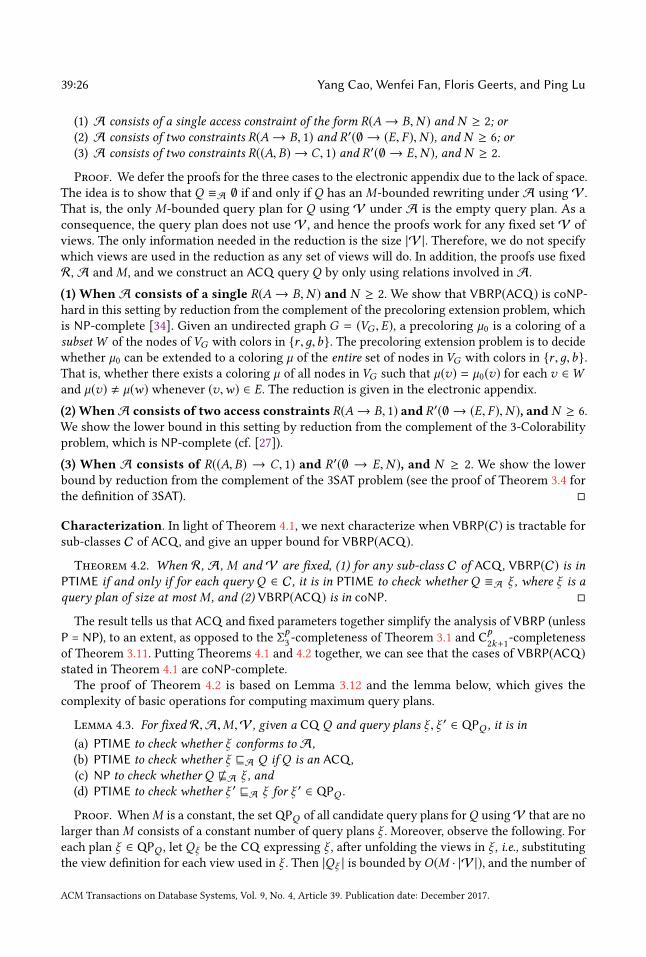
39:26 Yang Cao, Wenfei Fan, Floris Geerts, and Ping Lu
(1) A consists of a single access constraint of the form R(A → B,N ) and N ≥ 2; or(2) A consists of two constraints R(A → B, 1) and R′(∅ → (E, F ),N ), and N ≥ 6; or(3) A consists of two constraints R((A,B) → C, 1) and R′(∅ → E,N ), and N ≥ 2.
Proof. We defer the proofs for the three cases to the electronic appendix due to the lack of space.
The idea is to show that Q ≡A ∅ if and only if Q has anM-bounded rewriting under A usingV .
That is, the only M-bounded query plan for Q using V under A is the empty query plan. As a
consequence, the query plan does not use V , and hence the proofs work for any fixed set V of
views. The only information needed in the reduction is the size |V|. Therefore, we do not specify
which views are used in the reduction as any set of views will do. In addition, the proofs use fixed
R, A andM , and we construct an ACQ query Q by only using relations involved in A.
(1) When A consists of a single R(A → B,N ) and N ≥ 2. We show that VBRP(ACQ) is coNP-hard in this setting by reduction from the complement of the precoloring extension problem, which
is NP-complete [34]. Given an undirected graph G = (VG ,E), a precoloring µ0 is a coloring of a
subsetW of the nodes ofVG with colors in {r ,д,b}. The precoloring extension problem is to decide
whether µ0 can be extended to a coloring µ of the entire set of nodes in VG with colors in {r ,д,b}.That is, whether there exists a coloring µ of all nodes in VG such that µ(v) = µ0(v) for each v ∈Wand µ(v) , µ(w) whenever (v,w) ∈ E. The reduction is given in the electronic appendix.
(2) WhenA consists of two access constraints R(A → B, 1) and R′(∅ → (E, F ),N ), and N ≥ 6.
We show the lower bound in this setting by reduction from the complement of the 3-Colorability
problem, which is NP-complete (cf. [27]).
(3) When A consists of R((A,B) → C, 1) and R′(∅ → E,N ), and N ≥ 2. We show the lower
bound by reduction from the complement of the 3SAT problem (see the proof of Theorem 3.4 for
the definition of 3SAT). □
Characterization. In light of Theorem 4.1, we next characterize when VBRP(C) is tractable forsub-classes C of ACQ , and give an upper bound for VBRP(ACQ).
Theorem 4.2. When R, A, M and V are fixed, (1) for any sub-class C of ACQ , VBRP(C) is inPTIME if and only if for each query Q ∈ C, it is in PTIME to check whether Q ≡A ξ , where ξ is aquery plan of size at mostM , and (2) VBRP(ACQ) is in coNP. □
The result tells us that ACQ and fixed parameters together simplify the analysis of VBRP (unless
P = NP), to an extent, as opposed to the Σp3-completeness of Theorem 3.1 and Cp
2k+1-completeness
of Theorem 3.11. Putting Theorems 4.1 and 4.2 together, we can see that the cases of VBRP(ACQ)
stated in Theorem 4.1 are coNP-complete.
The proof of Theorem 4.2 is based on Lemma 3.12 and the lemma below, which gives the
complexity of basic operations for computing maximum query plans.
Lemma 4.3. For fixed R,A,M,V , given a CQ Q and query plans ξ , ξ ′ ∈ QPQ , it is in(a) PTIME to check whether ξ conforms to A,(b) PTIME to check whether ξ ⊑A Q if Q is an ACQ ,(c) NP to check whether Q @A ξ , and(d) PTIME to check whether ξ ′ ⊑A ξ for ξ ′ ∈ QPQ .
Proof. WhenM is a constant, the set QPQ of all candidate query plans forQ usingV that are no
larger thanM consists of a constant number of query plans ξ . Moreover, observe the following. For
each plan ξ ∈ QPQ , let Qξ be the CQ expressing ξ , after unfolding the views in ξ , i.e., substitutingthe view definition for each view used in ξ . Then |Qξ | is bounded byO(M · |V|), and the number of
ACM Transactions on Database Systems, Vol. 9, No. 4, Article 39. Publication date: December 2017.

BoundedQuery Rewriting Using Views 39:27
variables inQξ is at mostO(M · |V| · |R|). Recall that each element query ofQξ can be represented
asQξ ∧ϕ, where ϕ is a conjunction of equality atoms between variables used inQξ (see the proof of
Theorem 3.4). HenceQξ has 2O ((M · |V | · |R |)2)
many element queries. When R,A,M andV are fixed,
O(M · |V| · |R|) and 2O ((M · |V | · |R |)2)
are bounded by constants. Hence the size of Qξ is a constant,
and Qξ has a constant number of element queries. Similarly, we can show that Q has 2O ( |Q |2)
many
element queries, i.e., exponentially many.
We next verify the claims of Lemma 4.3 one by one.
(a) We use the algorithm given in the proof of Lemma 3.8 to check whether ξ conforms to A. We
show that the algorithm is in PTIME for CQ in this setting. It suffices to show that its step (3) is
in PTIME here instead of coNP. For each fetch(X ∈ S j ,R,Y ) operation in ξ , let ξ1 be the sub-tree
of ξ rooted at S j , and rewrite ξ1 into a CQ Q1 by unfolding views in ξ1. As shown above, Q1 has a
constant number of element queries, and the size of each element query is bounded by a constant.
Then by Lemma 3.7, step (3) of the algorithm can be done in PTIME. Thus checking whether ξconforms to A is in PTIME.
(b) It is easy to show that ξ ⊑A Q if and only if for each element query Qe of Qξ , Qe ⊑ Q (see the
proof of Theorem 3.4). Since Q is an ACQ , one can check whether Qe ⊑ Q in O(|Q | · |Qe |2) time,
by using the Acyclic Containment algorithm from [18]. As Qξ has a constant number of element
queries, checking whether ξ ⊑A Q is in PTIME. Note that if Q is a CQ instead of an ACQ , this is
not in PTIME.
(c) In contrast, Q has 2O ( |Q |2)
element queries, and checking whether Q @A ξ is in NP, rather thanin PTIME as in (b). This can be done as follows: guess an element queryQe ofQ , and check whether
Qe @ ξ . As remarked earlier, ξ can be expressed by a CQ Qξ of size bounded by a constant. Thus
the number of candidate homomorphic mappings from Qξ to Qe is at most O(|Qe ||Qξ |), which is a
polynomial. Thus we can check Qe @ Qξ in PTIME by enumerating all candidate mappings and
verifying whether one of them is indeed a homomorphism from Qξ to Qe . Hence it is in NP to
check whether Q @A ξ .
(d) For any ξ ′ ∈ QPQ , we first rewrite ξ ′ into a query Qξ ′ in CQ by unfolding views in ξ ′. Thenξ ′ ⊑A ξ if and only if Qξ ′ ⊑A Qξ . As argued above, Qξ ′ has a constant number of element queries,
andQξ and all element queries ofQξ ′ have a constant size. Hence checkingQξ ′ ⊑A Qξ is in PTIME,and so is checking ξ ′ ⊑A ξ . □
Proof of Theorem 4.2. Based on the lemmas, we prove Theorem 4.2. We first present an algorithm,
denoted by AlgACQ , to check whether an ACQ Q has anM-bounded rewriting. For fixed R, A,Mand V , we show that the algorithm is in coNP for general ACQ queries. However, when we focus
on specific sub-classes C of ACQ , the algorithm runs in PTIME. More specifically, classes C have
the following property: for each query Q ∈ C, it is in PTIME to check whether Q ≡A ξ . Here, ξ is
a query plan of size at mostM .
From Lemma 3.12, we know that a query Q has anM-bounded rewriting under A usingV if
and only if there exists a unique maximum query plan ξ ∈ QPQ (up to A-equivalence) such that
Q ⊑A ξ . To develop AlgACQ , we first show that given any ACQ Q , its unique maximum plan ξ (up
to A-equivalence) can be computed in PTIME, if it exists. It is computed by the algorithm given
below, denoted by AlgMP:
(1) generate the set QPQ of all candidate query plans for Q of length at mostM , using relation
atoms in R and views in V;
ACM Transactions on Database Systems, Vol. 9, No. 4, Article 39. Publication date: December 2017.

39:28 Yang Cao, Wenfei Fan, Floris Geerts, and Ping Lu
(2) remove from QPQ all plans ξ ∈ QPQ such that its CQ query Qξ is not acyclic;
(3) remove from QPQ all ξ ∈ QPQ such that ξ @A Q or ξ does not conform to A;
(4) remove from QPQ all query plans ξ ∈ QPQ such that there exists another query plan ξ1
satisfying ξ1 ⊑A Q and ξ ⊏A ξ1;
(5) if QPQ is nonempty and all remaining plans in QPQ are A-equivalent to each other, return a
plan ξ in QPQ ; otherwise return “no”.
The correctness of algorithm is obvious. For its complexity, step (1) is in PTIME since there exist
a constant number of plans in QPQ , and each of them has size bounded by a constant. Step (2) is in
PTIME since checking whether a CQ query is acyclic can be done in PTIME by using, e.g., GYOalgorithm [48]). Step (3) consists of (i) checking whether ξ conforms toA; and (ii) checking whether
ξ @A Q . These are in PTIME by Lemma 4.3(a) and (b). Step (4) checks A-containment between
query plans and A-containment of queries plans in Q . These are in PTIME by Lemma 4.3(b) and
(d). In contrast, when Q is CQ , steps (3) and (4) have to call an NP oracle for a constant number
of times. This explains why VBRP(ACQ) differs from VBRP(CQ) (Theorem 3.11) unless P = NP.Step (5) checks A-containment of query plans, in PTIME by Lemma 4.3(d). Putting these together,
algorithm AlgMP is in PTIME.Capitalizing on AlgMP, algorithm AlgACQ works as follows. Given an ACQ Q , it first checks
whether Q has a unique maximum plan ξ in QPQ , by invoking AlgMP. If such a query plan does
not exist, then Q does not have anM-bounded query rewriting by Lemma 3.12, and hence AlgACQreturns false. Otherwise, it checks whether Q ≡A ξ ; it returns true if so, and false otherwise.
We now prove the two statements of Theorem 4.2 by analyzing AlgACQ .
(1) Sub-classes C. Consider a sub-class C of ACQ such that for each Q ∈ C, checking whether
Q ≡A ξ is in PTIME. As argued above, AlgMP is in PTIME. Then AlgACQ is in PTIME, and hence so
is VBRP(C). Conversely, givenQ ∈ C and ξ , we can check whetherQ ≡A ξ as follows: (1) compute
a unique maximum plan ξQ ∈ QPQ ; (2) check whether ξQ ≡A ξ andQ has anM-bounded rewriting;
return true if so, and false otherwise. The correctness and time complexity follow from Lemmas 3.12,
4.3(c), (d), and the assumption that VBRP(C) is in PTIME. In fact, to ensure that VBRP(C) is inPTIME, we only need to show that deciding Q ⊑A ξ is in PTIME. Indeed, by Lemma 4.3, checking
ξ ⊑A Q is in PTIME, and hence we also have that deciding Q ≡A ξ is in PTIME. However, theconverse does not hold. That is, when VBRP(C) is in PTIME, it is not necessary that deciding
Q ⊑A ξ is in PTIME. In particular, if ξ @A Q and ifQ has noM-bounded rewriting, then we cannot
further infer that Q ⊑A ξ .
(2) ACQ . For a general query Q in ACQ , checking whether Q ⊑A ξ is in coNP by Lemma 4.3(c).
Since AlgMP is in PTIME, AlgACQ is in coNP, and so is VBRP(ACQ).
This concludes the proof of Theorem 4.2. □
Theorem 4.2 helps us identify sub-classes of ACQ for which VBRP is tractable, such as ACQunder “FDs”, i.e., when all the access constraints in A are of the form R(X → Y , 1). As remarked
earlier, FDs with associated indices are common access constraints, and can be discovered by using
existing tools for mining FDs (e.g., [33]).
Corollary 4.4. When R,A,M andV are fixed, VBRP is in PTIME for ACQ if A consists of FDsonly.
Proof. By Theorem 4.2, it suffices to show that checking whether Q ⊑A ξ is in PTIME, where ξdenotes the unique maximum query plan, if it exists.
Given a set A of access constraints of the FD form and an ACQ Q , we chase the tableau T of Qby A as follows [4]: for each R(X → Y , 1) ∈ A, if there exist tuples R(x , y1, z1) and R(x , y2, z2) in
T such that (a) x corresponds to X , and (b) y1 and y2 correspond to Y , and y1 , y2, then we unify
ACM Transactions on Database Systems, Vol. 9, No. 4, Article 39. Publication date: December 2017.

BoundedQuery Rewriting Using Views 39:29
y1 = y2 in T . These yield a tableau TA satisfying A. Let QAbe the query expressed by TA . One
can see that QAis unique up to homomorphism [38], QA ≡A Q and QA
satisfies A.
Observe the following: (a)Q ⊑A ξ is equivalent toQA ⊑ ξ ; the latter is in terms of conventional
query containment ⊑; and (b) QA ⊑ ξ can be checked in PTIME since ξ is of constant size. Indeed,
at mostO(|QA | |ξ |) homomorphic mappings need to be checked. From these it follows that whether
Q ⊑A ξ can be checked in PTIME. □
In contrast to Corollary 4.4, VBRP remains intractable for CQ under FDs, although the analysis
is simpler compared with Theorem 3.11 (unless P = NP).
Proposition 4.5. For fixed R,A,M andV , VBRP(CQ) is NP-complete even when A consists ofFDs only. It remains NP-complete when none of R,A,M and V is fixed.
Proof. We first show the lower bound, followed by the upper bound.
Lower bound. We show that in this setting, VBRP(CQ) is NP-hard by reduction from the 3SATproblem (see the proof of Theorem 3.4 for 3SAT). Given an instance ψ of 3SAT, we define a CQQ , an access schema A of the FD form, a boundM , and a setV of CQ views, such that Q has an
M-bounded rewriting in CQ using V under A if and only ifψ is satisfiable. We ensure thatM,A,
R andV do not depend onψ , i.e., they are fixed.
(1) The database schema R consists of R∨(B,A1,A2), R∧(B,A1,A2) and R¬(A, A) to encode the
Boolean operations, as in the proof of Theorem 3.4 (see Figure 2). Observe that we do not include
R01 in R. The reason is that we cannot enforce instances of R01 to coincide with I01 (see Figure 2)
using access constraints of the FD form.
(2) The access schema A contains the following three constraints to ensure that R∨, R∧, R¬ can
be used to encode the Boolean operations: R∨((A1,A2) → B, 1),R∧((A1,A2) → B, 1),R¬(A → A, 1).All these constraints have the form of R(X → Y , 1).
(3) The query Q is defined as Q() = Qc () ∧Qψ (x , 1), where (a) Qc () is the same as its counterpart
given in the proof of Theorem 3.4, except for the sub-query in Qc related to R01. It is to ensure that
the instances of R∨, R∧, and R¬ contain all the tuples shown in Figure 2, and (b) Qψ (x , 1) is similar
to its counterpart given in the proof of Theorem 3.4, to encode all truth assignments µ of x such
thatψ (µ(x)) = true, expressed in terms of R∨, R∧ and R¬. In contrast to the query used in the proof
of Theorem 3.4, Qψ extracts the Boolean domain from R¬ rather than R01. Note that if an instance
D of R is equal to the instances shown in Figure 2 (excluding I01), then Q(D) is nonempty if and
only ifψ is satisfiable. Of course, when D is an instance of R that satisfies A but it contains more
tuples than those shown in Figure 2, Qc (D) , ∅ and Q(D) = ∅ still ensure thatψ is unsatisfiable,
butQc (D) , ∅ andQ(D) , ∅ do not imply thatψ is satisfiable. Indeed, x may be non-Boolean, and
Qψ does not correctly evaluateψ in this case.
(4) The set V consists of a single CQ view: V () = Qc (), which is the same as the one given in Q .Finally, we letM = 1.
Since all access constraints in A are FDs andM = 1, the only possible query plans are ∅ and V .
One can verify that Q has an 1-bounded rewriting in CQ using V under A if and only if V ≡A Qif and only ifψ is true. Note thatM,A, R andV are fixed.
Upper bound. We give the following NP algorithm to check VBRP(CQ) when none of R,A,V and
M is fixed, and when A consists of FD-like access constraints only:
ACM Transactions on Database Systems, Vol. 9, No. 4, Article 39. Publication date: December 2017.

39:30 Yang Cao, Wenfei Fan, Floris Geerts, and Ping Lu
(1) chase the tableau TQ of Q by A as described in the proof of Corollary 4.4; this yields tableau
TQ1that satisfies A; let Q1 be the CQ represented by TQ1
;
(2) guess a query plan ξ such that |ξ | ≤ M , a CQ query Q2 such that the tableau of Q2 satisfies
A and |Q2 | ≤ M · |V | · |R |, a homomorphism h1 from Q1 to Q2, and a homomorphism h2
from Q2 to Q1;
(3) check whether ξ conforms to A; if not, then reject the guess; otherwise, continue;
(4) rewrite ξ into a CQ query Q ′by unfolding views in ξ ;
(5) chase the tableau TQ ′ of Q ′by A, which yields TQ ′
1
that satisfies A;
(6) syntactically check whether the tableauTQ2of Q2 is the same asTQ ′
1
, i.e., a tuple template t isin TQ2
if and only if t is in TQ ′1
; if not, then reject the guess; otherwise, continue;
(7) check whether h1 and h2 are homomorphic mappings, and whether h1 witnesses Q2 ⊑ Q1
and h2 witnesses Q1 ⊑ Q2; if so, return true; otherwise reject the guess.
The algorithm is obviously correct. For its complexity, we need the following Lemma.
Lemma 4.6. If A consists of FDs only, it is in PTIME to decide whether a plan ξ ∈ QPQ conformsto A. □
Using the lemma, we show that the algorithm for VBRP(CQ) is in NP. Since the chase can be
done in PTIME, steps (1) and (5) are in PTIME. By Lemma 4.6, step (3) can be done in PTIME. Step(4) is in PTIME. Step (6) does syntactic checking and is in PTIME. Because homomorphic mappings
can be verified in PTIME, step (7) is also in PTIME.This concludes the proof of Proposition 4.5, modulo the proof of Lemma 4.6. □
We next verify Lemma 4.6.
Proof of Lemma 4.6. To check whether ξ conforms to A, we check whether for each fetch(X ∈
S j ,R,Y ) operation in ξ , the following conditions hold: (a) there is an access constraint R(X → Y ′, 1)in A such that Y ⊆ X ∪ Y ′
; and (b) there exists a constant N such that for all instances D of R
that satisfy A, |S j | ≤ N in the computation of ξ (D).
For each fetch(X ∈ S j ,R,Y ) operation, it is in PTIME to check condition (a). We use the following
algorithm to check condition (b). Let ξ j be the sub-tree of ξ rooted at S j , and Q j be the query
expressed by ξ j . The algorithm works as follows:
(1) unfold Q j by replacing each view with its definition, yielding Q ′j in CQ;
(2) chase the tableauTQ ′jofQ ′
j byA as described in the proof of Corollary 4.4; this yields tableau
TQ ′′jthat satisfies A; let Q ′′
j be the CQ represented by TQ ′′j;
(3) check whether Q ′′j has bounded output; if so, return true; otherwise, return false.
From the proof of Corollary 4.4, we can see that Q ′′j ≡A Q j . Then the correctness of the algorithm
follows. For its complexity, observe that step (1) is in PTIME. Since the chase can be done in PTIME,step (2) is in PTIME. Because the tableau TQ ′′
jsatisfies A, and computing cov(Q ′′
j ,A) is in PTIME,step (3) is in PTIME by Lemma 3.6. Since there are at mostO(|ξ |) fetch operations in ξ , the algorithmis in PTIME. □Along the same lines as Corollary 4.4, one can verify that for fixed R,A,M and V , VBRP is
in PTIME for the sub-class of ACQ queries such that their tableau representations satisfy the
cardinality constraints in A. A special case of this is when A = ∅, e.g., the setting of [7], when
access constraints are not employed at all.
Theorem 4.2 remains intact on any class C of queries as long as it is in PTIME to compute a
maximum plan in QPQ for all queries in C. Examples include
(1) self-join-free CQ , i.e., the class of CQ queries that contain no repeated relation names, and
ACM Transactions on Database Systems, Vol. 9, No. 4, Article 39. Publication date: December 2017.
BoundedQuery Rewriting Using Views 39:31
(2) CQ with a fixed number of variables, i.e., for each constant k , the class of CQ queries that
have at most k free variables.
By Theorem 4.2 and Lemma 4.3, VBRP is also in PTIME in these two cases.
The results of the section tell us that the intractability of VBRP(ACQ) is robust. The proof of
Theorem 4.1 shows that A is the crucial parameter here, while V and M could be empty and 0,
respectively. Not all is lost. There are practical cases when VBRP(ACQ) and even VBRP(CQ) are
tractable. Moreover, we can cope with the hardness by means of effective syntax (Section 5) and
approximate query answering (Section 8).
5 AN EFFECTIVE SYNTAXWe have seen that the undecidability of VBRP for FO and the intractability for CQ are rather robust.
Can we still make practical use of bounded rewriting analysis when querying big data? We next
show that the answer is affirmative.
We develop effective syntax for FO queries that have a bounded rewriting, to syntactically
check the existence of bounded rewriting in PTIME without sacrificing the expressive power. More
specifically, for any database schema R, views V , access schema A and bound M , we identify two
classes of FO queries, (a) a class of queries topped by (R,V,A,M), which “covers” all FO queries
over R that have anM-bounded rewriting using V under A, up to A-equivalence, and (b) a class
of size-bounded queries, which “covers” all the views of V in FO that have bounded output for all
instances D |= A of R. The second class is to effectively check bounded output (see Section 3.1).
We show that it is in PTIME to syntactically check whether a query is topped or size-bounded.
Below we first present the main results of the section in Section 5.1. We then define topped
queries and size-bounded queries in Sections 5.2 and 5.3, respectively.
5.1 Practical Use of Bounded RewritingThe main results of the section are as follows.
Theorem 5.1. For any R,V andM , and under any A,
(a) each FO query Q with anM-bounded rewriting using V is A-equivalent to a query topped by(R,V,A,M);
(b) every FO query topped by (R,V,A,M) has anM-bounded rewriting in FO using V under A,which can be identified in PTIME inM , |Q |, |V| and |A|; and
(c) it takes PTIME in M, |R |, |Q |, |V| and |A| to check whether an FO query Q is topped by(R,V,A,M), which uses an oracle that checks whether FO views inV have bounded outputin PTIME in |Q |.
Here A, Q and V are all defined over the same R. □
That is, topped queries are a key sub-class of FO queries with a bounded rewriting, and can
be efficiently checked. Moreover, the bounded rewriting can also be efficiently generated. For the
existence of the oracle, we show the following.
Theorem 5.2. For any R and under any A,
(a) each FO query Q over R that has bounded output is A-equivalent to a size-bounded queryunder A;
(b) each size-bounded query has bounded output under A; and(c) it takes PTIME in |Q | to check whether an FO query Q is a size-bounded query.
Here A and Q are defined over the same R. □
ACM Transactions on Database Systems, Vol. 9, No. 4, Article 39. Publication date: December 2017.
39:32 Yang Cao, Wenfei Fan, Floris Geerts, and Ping Lu
Before we define topped and size-bounded queries, we remark the following. (1) Theorems 5.1
and 5.2 just aim to demonstrate the existence of effective syntax for FO queries with bounded
rewriting. There are other forms of effective syntax for such FO queries. (2) Theorem 5.1 does not
contradict to Corollary 3.9 due to the requirement of A-equivalence in its condition (a), which is
undecidable for FO.
Practical use of bounded query rewriting. Capitalizing on the effective syntax, we can develop
algorithms (a) to check whether a given FO query Q is topped by (R,V,A,M) in PTIME; and if
so, (b) to generate a bounded query plan ξ for Q using V . The existence of these algorithms is
warranted by Theorems 5.1 and 5.2.
We can then support bounded rewriting on top of commercial DBMS as follows. Given an
application, a database schema R and a resource bound M are first determined, based on the
application and available resources, respectively. Then, a setV of views can be selected following [7],
and a set A of access constraints can be discovered. After these are in place, given an FO query Qposed on an instance D of R that satisfiesA, we check whetherQ is topped by (R,V,A,M). If so,
we generate a bounded query plan ξ forQ usingV , by using the algorithms described above. Then
we can compute Q(D) by executing ξ with the existing DBMS. Since a commercial DBMS may not
execute ξ directly, this can be carried out by translating ξ into an equivalent SQL query Qξ , which
is passed to the underlying DBMS, as suggested in [11]. By “implementing” fetch operations in
terms of index joins and using join hints or virtual views to enforce the join orders, we can enforce
DBMS to evaluate Qξ by exactly following ξ . Moreover, incremental methods for maintaining the
views [7] and the indices of A [11] have already been developed, in response to updates to D.
Putting these together, we can expect to efficiently answer a number of FO queries in (possibly big)
D by leveraging bounded rewriting.
5.2 ToppedQueries for Bounded RewritingWe next define topped queries and outline a proof of Theorem 5.1.
It is nontrivial to define an effective syntax, as shown below.
Example 5.3. Consider a database schema R1 with two relations R(A,B) and T (C,E), an access
schema A2 consisting of R(A → B,N ) and T (C → E,N ), and V3 with a single view V3(x ,y) =R(y,y) ∧T (x ,y). Given a value for x , V3 returns a bounded number of y values due to the access
constraint on T . Consider FO query: q3(z) = q4(z) ∧ ¬∃w R(z,w), where q4(z) = ∃x∃y ((R(y,y) ∧T (x ,y)) ∧ (x = 1)) ∧ R(y, z). Then q3 has a 13-bounded rewriting as in Fig. 3, which is for an
A-equivalent query:
q′3(z) = q4(z) ∧ ¬(q4(z) ∧ ∃w R(z,w)).
Observe the following. (1) Query q′3becomes bounded because it propagates z-values from q4 to
“¬∃w R(z,w)”. (2) Such propagated values allow us to fetch bounded data for relation atoms, i.e.,R(z,w). (3) The part of the plan for a sub-query of q3 may have to embed the part of the plan for
another sub-query. For instance, (i) q4 has a 5-bounded rewriting in q3 (the left part of Fig. 3); (ii)
∃w R(z,w) has a 7-bounded rewriting in q3 (the right part of Fig. 3), which embeds the 5-bounded
plan for q4; and (iii) the size of the plan for q3 is the sum of the sizes of plans for q4 and ∃w R(z,w),
i.e., 5 + 7 + 1 = 13.
This shows that to cover queries such as q3, topped queries have to support value propagation
among sub-queries, and keep track of the sizes of plans for sub-queries. □
Topped queries. This observation motivates us to define topped queries by characterizing value
propagation among their sub-queries. To do this, we define topped queries with two binary functions
covq(Qs (x),Q(z)) and size((Qs (x),Q(z)) that take two queries Qs (x) and Q(z) as input parameters.
ACM Transactions on Database Systems, Vol. 9, No. 4, Article 39. Publication date: December 2017.

BoundedQuery Rewriting Using Views 39:33
S13 = S5 \ S12
S5 = πB (S4)
S4 = fetch(A ∈ S3,R,B)
S3 = πE (S2)
S2 = σC=1(S1)
S1 = V3
S12 = πB (S11)
S11 = fetch(A ∈ S10,R,B)
S10 = πB (S9)
S9 = fetch(A ∈ S8,R,B)
S8 = πE (S7)
S7 = σC=1(S6)
S6 = V3
Fig. 3. A bounded plan for q3 of Example 5.3.
Below we first provide intuition behind covq(Qs (x),Q(z)) and size((Qs (x),Q(z)). Using the func-
tions, we then define topped queries, and complete the definition by giving the syntactic form of
the two functions.
(1) Boolean function covq(Qs (x),Q(z)) returns true if the following condition holds: if covq(Qs (x),Q(z)) = true and Qs (x) has a bounded rewriting, then Qs (x) ∧Q(z) also has a bounded rewriting.
Intuitively, Q(z) is a (sub-)query we are inspecting, and Qs (x) keeps track of sub-queries from
which values are propagated to Q(z).We use covq(Qs (x),Q(z)) to check whether we can propagate values from Qs to Q , and get
a bounded rewriting of Q in Qs ∧ Q . For instance, by covq(q4(z),∃w R(z,w)) = true for q3(z) inExample 5.3, in which q4(z) isQs and ∃w R(z,w) isQ , it indicates that if q4 has a bounded rewriting,
then by propagating values to free variable z of q4, we can have a bounded rewriting for sub-query
∃w R(z,w) in q4(z) ∧ ∃w R(z,w).
Note that only values of the free variables of Qs (x) can be propagated to Q(z), and Q(z) can only
take values for its free variables as input from Qs (x). In other words, Q(z) only takes values of the
variables in x ∩ z from Qs (x).In particular, Qs may include views from V . As will be shown shortly, function covq(Qs ,Q)
distinguishes views that need to have bounded output from those that do not have to, to ensure
that a bounded number of values are propagated from Qs to Q over any instance D |= A, i.e., Qdoes have a bounded rewriting sub-plan in Qs ∧Q .
(2) Function size((Qs (x),Q(z)) is a natural number that maintains an upper bound of the size of
minimum sub-plans for sub-query Q(z) in Qs (x) ∧Q(z). We will use size(Qs ,Q) to ensure that our
query plans do not exceed a given boundM .
For instance, in Example 5.3, size(q4,∃w R(z,w)) = 7, which is the size of the sub-plan for
evaluating ∃w R(z,w) in q4 ∧ ∃wR(z,w) by using values propagated from q4.
We now define topped queries using the two functions. An FO query Q over R is topped by (R,V,A,M) if (1) covq(Qϵ ,Q) = true; and (2) size(Qϵ ,Q) ≤ M . Here Qϵ is a “tautology query” such
that for anyQ ,Qϵ ∧Q =Q andQϵ has a 0-bounded plan. It is an extension of functions covq(Qs ,Q)and size(Qs ,Q) for function parameter Qs .
Intuitively, we compute covq(Qs ,Q) and size(Qs ,Q) starting with Qs = Qϵ , and conclude that Qis topped by (R,V,A,M) if the two conditions above are satisfied.
Functions covq(·, ·) and size(·, ·). We next define the functions inductively based on the structure
of FO queryQ . In the process, we also give a bounded query plan. We will ensure that if covq(Qs (x),
ACM Transactions on Database Systems, Vol. 9, No. 4, Article 39. Publication date: December 2017.

39:34 Yang Cao, Wenfei Fan, Floris Geerts, and Ping Lu
Q(z)) = covq(Qϵ ,Qs (x)) = true and Qs (x) has a size(Qϵ ,Qs (x))-bounded rewriting, then Qs (x) ∧Q(z) has a size(Qϵ ,Qs (x) ∧Q(z))-bounded rewriting.
The definition of covq(Qs (x),Q(z)) and size(Qs (x),Q(z)) is separated into 7 cases below. In
particular, we define covq(Qs (x),Qϵ ) = true, size(Qs (x),Qϵ ) = 0.
(1) Q(z) is z = c . We define covq(Qs (x),Q(z)) = true and size(Qs (x),Q(z)) = 1.
(2) Q(z) is V (z).We can access cached views; thus, we define covq(Qs (x),Q(z)) = true and size(Qs (x),
Q(z)) = 1. That is, constant queries and views have 1-bounded rewriting and therefore, are taken as
topped queries.
(3) Q(z) is Q ′(z) ∧C , where C is one of (x = y), (x , y), (x = c) and(x , c). We define covq(Qs (x),
Q(z)) = covq(Qs (x),Q′(z)); and size(Qs (x),Q(z)) = size(Qs (x),Q
′(z)) + 1 when covq(Qs (x),Q′(z))
= true, and as size(Qs (x),Q(z)) = +∞ otherwise. Given a bounded plan ξ ′ for Q ′, a bounded plan
for Q is (T = ξ ′,σC (ξ′)), increasing the size of ξ ′ by 1.
(4) Q(z) is Q1(z1) ∧Q2(z2), where Q2 is not an (in)equality. Here, let µi = covq(Qs (x),Qi (zi )), si =
size(Qs (x),Qi (zi )), s = size(Qϵ ,Qs (x)), µ′ = covq(Qs (x) ∧Q1(z1),Q2(z2)), s
′ = size(Qs (x) ∧Q1(z2),Q2(z2)) (i ∈ {1, 2}). We distinguish the following cases:
(a) if µ1 = true,Q2(z2) is of the form ∃w R(z1, z′2, w), there exists access constraint R(Z1 → Z ′
2,N )
is in A with Z1 ∪ Z ′2= Z2 and if Qs (x) ∧Q1(z1) has bounded output under A, then we define
covq(Qs (x),Q(z)) = true and size(Qs (x),Q(z)) = s1 + 1; otherwise
(b) if µ1 = µ2 = true, then covq(Qs (x),Q(z)) = true, size(Qs (x),Q(z)) = 2s + s1 + s2 + λ(z1, z2),
where λ(z1, z2) is 1 (resp. 4) if z1 ∩ z2 is empty (resp. not empty); otherwise
(c) if µ1 = µ′ = true and |Q2 | ≤ K for some predefined constant K (here |Q2 | is the size of Q2),
then covq(Qs (x),Q(z)) = true and size(Qs (x),Q(z)) = s1 + s′.
(d) otherwise we define covq(Qs (x),Q(z)) = false and size(Qs (x),Q(z)) = +∞.
In case (4) we characterize value propagation via conjunction in the queries. More specifically,
when covq(Qs (x),Q(z)) = true, we have three cases below.
(a) If Q1 has a bounded plan ξ1 with Qs , and if Q2 is (a projection of) a relation atom covered by an
access constraint R(Z1 → Z ′2,N ) in A, then Q(z) also has a bounded plan with Qs (x) and Q1(z1),
as long as Qs (x) ∧Q1(z1) has bounded output. Indeed, a plan for Q2 is (T = ξ1, fetch(X ∈ T ,R,Z ′2))
of size |ξ1 | + 1. We instantiate the Z1 attributes of R with the output of Q1(z1), and ensure that the
input T of fetch, i.e., the output of Qs (x) ∧Q1(z1), has bounded size. This case requires bounded
output analysis.
For instance, consider q2 = ∃x ((R(y,y) ∧T (x ,y)) ∧ (x = 1)) and R(y, z) in sub-query q4 of q3 of
Example 5.3. The y-values from q2 are propagated to R(y, z) in this case.
By cases (2), (3) and (7c) (will be seen shortly), one can verify that covq(Qϵ ,q2) = true and
size(Qϵ ,q2) = 2 under A2 and V3 of Example 5.3. Now consider query q′2= q2 ∧ R(y, z). By case
(4a), we have that covq(Qϵ ,q′2) = covq(Qϵ ,q2) = true and size(Qϵ ,q
′2) = size(Qϵ ,q2) + 1 = 3. Thus
q′2is topped by (R1,V3,A2, 3) (recall R1, V3 and A2 from Example 5.3).
(b) If both Q1 and Q2 have bounded sub-plans with Qs , e.g., ξ1 and ξ2, respectively, then Q also
has a bounded plan with Qs , whose size depends on the forms of Q1(z1) and Q2(z2), as reflected in
different values of λ(z1, z2). More specifically, if z1 and z2 are disjoint, then Q is a production of Q1
and Q2 and thus has a query plan (T1 = ξ1, T2 = ξ2, T3 = T1 ×T2), of size |ξ1 | + |ξ2 | + 1. Otherwise,
i.e., if z1 ∩ z2 , ∅, then Q is a join of Q1 and Q2 and thus has a plan (T1 = ξ1, T2 = ξ2, T3 = ρ(T2),
T4 = T1 ×T2, T5 = σZ1∩Z2=ρ(Z1∩Z2)(T4)), of size |ξ1 | + |ξ2 | + 4. Here ρ renames attributes in Z1 ∩ Z2.
Note that ξ1 and ξ2 are sub-plans of Q1 and Q2 with Qs , respectively, which use the output of Qs to
ACM Transactions on Database Systems, Vol. 9, No. 4, Article 39. Publication date: December 2017.

BoundedQuery Rewriting Using Views 39:35
computeQ1 andQ2. Hence, |ξ1 | and |ξ2 | are characterized by s +s1 and s +s2, respectively, including
the size of the plan for Qs .
For example, consider Qs = S(x), Q1 = R(x ,y) and Q2 = R(x , z) over relation schemas S(C) and
R(A,B) with access constraints S(∅ → C,N ) and R(A → B,N ). Then covq(Qs ,Q1 ∧ Q2) = truesince covq(Qs ,Q1) = covq(Qs ,Q2) = true (by cases (7a) and (7b), which will be discussed shortly);
size(Qs ,Q1 ∧ Q2) = B1 + B2 + 4, where Bi = size(Qϵ ,Qs ) + size(Qs ,Qi ) (for i = 1, 2) is an upper
bound of the size of the sub-plan for Qi with Qs that will be used by the plan for Q with Qs ; and 4
is the number of steps to join sub-plans for Q1 and Q2 with Qs together. Note that size(Qϵ ,Qs ) is
counted twice as it will be used by the sub-plans for both Q1 and Q2 with Qs .
(c) If Q1 has a bounded plan with Qs while Q2 has a bounded plan with Qs ∧ Q1 instead of Qsalone, e.g., plans ξ1 and ξ
′2, respectively, then Q has a bounded query plan of size |ξ1 | + |ξ ′
2|, where
|ξ1 | = size(Qs (x),Q1(z1)) and |ξ ′2| = size(Qs ∧Q1(x),Q2(z2)). Note that we extendQs (x)withQ1(z1)
only if Q1(z1) has a bounded plan usingV with Qs (i.e., covq(Qs ,Q1) = true). One can verify that
this expansion policy assures that Qs always has a bounded plan since we start with a tautology
query Qs = Qϵ .
Observe the following. (1) Qs is expanded in case (c) above to propagate z1 from Q1 ∧Qs to Q2
there. More specifically, if sub-query Q2(z2) of Q does not have a bounded rewriting with Qs (x)(i.e., when µ2 = false), we may extend Qs (x) with Q1(z1) to make Q2(z2) bounded when µ ′ = true.(2) We also restrict the size |Q2 | for case (c) to ensure both functions covq(·, ·) and size(·, ·) arein PTIME. Indeed, to compute covq(Qs ,Q), we need to expand Qs with various conjuncts of Q2
if Q2 is also a conjunction, by applying case (4b) or (4c) alternatively. For example, when Q2 is
Q21 ∧Q22, to compute covq(Qs ,Q) via cases (4b) and (4c), we may need to compute covq(Qs ,Q22),
covq(Qs ∧Q1,Q22), covq(Qs ∧Q21,Q22) and covq(Qs ∧Q1 ∧Q21,Q22). In the worst case, we may
test 2|Q2 |
many difference cases. Hence we restrict the size of Q2 by a predefined constant K , tobound the number of expansions ofQs when computing covq(Qϵ ,Q) and ensure that it is in PTIME.We remark that this restriction has no impact on the expressive power of topped queries up to
equivalence, even when K = 1 (see the proof of Theorem 5.1 in the electronic appendix for more
details).
(5) Q(z) is Q1(z1) ∨Q2(z2). If z1 , z or z2 , z, we let covq(Qs (x),Q(z)) = false and size(Qs (x),
Q(z)) = +∞. Otherwise, let µi = covq(Qs (x),Qi (z)) and si = size(Qs (x),Qi (z)) for i ∈ {1, 2}. Definecovq(Qs (x),Q(z)) = µ1 ∧ µ2, and size(Qs (x),Q(z)) = s1 + s2 + 1 if covq(Qs (x),Q(z)) = true and
size(Qs (x),Q(z)) = +∞ otherwise.
Intuitively, if Q1 and Q2 have bounded plans ξ1 and ξ2, respectively, then Q(z) has a boundedplan (T1 = ξ1,T2 = ξ2,T1 ∪T2), of size |ξ1 | + |ξ2 | + 1.
Note that when Q1 and Q2 do not share the same free variables z, Q1 ∨Q2 can never be topped
queries since covq(Qs ,Q1 ∨Q2) = false. This is to ensure that topped queries are safe-range and
hence are “safe”, i.e., domain-independent (only domain-independent calculus queries are well-
defined queries, i.e., queries have determined query answers on every database instance, and have
equivalent algebra forms and query plans [28]). For example, this will exclude “unsafe” queries like
Q(x ,y) = ∃w1,w2 R(w1,x) ∨ R(w2,y) from the class of topped queries.
(6) Q(z) is Q1(z1) ∧ ¬Q2(z2). If z1 , z or z2 , z, we define covq(Qs (x),Q(z)) = false and size(Qs (x),
Q(z)) = +∞. Otherwise, let µi = covq(Qs (x),Qi (z)), si = size(Qs (x),Qi (z)), µ12 = covq(Qs (x),Q1(z)∧Q2(z)), and s12 = size(Qs (x),Q1(z) ∧Q2(z)). Then we define
(a) if µ1∧ µ2= true, covq(Qs (x),Q(z)) = true and size(Qs (x),Q(z))=s1+s2+1; otherwise
ACM Transactions on Database Systems, Vol. 9, No. 4, Article 39. Publication date: December 2017.

39:36 Yang Cao, Wenfei Fan, Floris Geerts, and Ping Lu
(b) if µ1∧ µ12 = true and |Q2 | ≤ K for some predefined constant K , covq(Qs (x),Q(z)) = true and
size(Qs (x),Q(z)) = s1 + s12 + 1; otherwise
(c) we define covq(Qs (x),Q(z) = false and size(Qs (x),Q(z)) = +∞.
It is case (6) that captures how sub-query Q4 of Q3 is propagated to ∃w R(z,w) in Example 5.3.
When covq(Qs (x),Q(z)) = true, we have one of the following three cases.
(a) When µ1 = µ2 = true, it is similar to case (5) above.
(b) If µ1 = µ12 = true, let ξ1 and ξ12 be the plans forQ1(z) andQ1(z)∧Q2(z), respectively, withQs (x).SinceQ1(z)∧¬Q2(z) =Q1(z)∧¬(Q1(z)∧Q2(z)),Q(z) has bounded plan (T1 = ξ1,T2 = ξ12,T3 = T1−T2),
of size |ξ1 | + |ξ12 | + 1. For the same reason as the one given in case 4(c) above, we also require
|Q2 | ≤ K here.
(c) Otherwise, covq(Qs (x),Q(z)) = false, and thus size(Qs (x),Q(z)) = +∞, i.e., Q has no bounded
rewriting.
For the same reason as (5), we only allow cases when Q1 and Q2 have the same free variables to
be topped queries, to ensure that every topped query is safe-range.
(7) Q(z) is ∃w Q ′(w, z) (w is possibly empty). Let µ ′ = covq(Qs (x),Q′(w, z)) and s ′ = size(Qs (x),Q
′(w,
z)). Then we consider the following three cases:
(a) if Q ′is R(w, z) and there exists access constraint R(∅ → Z ,N ) ∈ A, then we define
covq(Qs (x),Q(z)) = true and size(Qs (x),Q(z)) = 1;
(b) if Q ′is R(w, z), R(X → Z ′,N ) ∈ A, X ∪ Z ′ = Z and if Qs (x) has bounded output under A,
then covq(Qs (x),Q(z))=true, size(Qs (x),Q(z)) = s′ + 1;
(c) otherwise, covq(Qs (x),Q(z)) = covq(Qs (x),Q′(w, z)) and size(Qs (x),Q(z)) = size(Qs (x),Q
′(w,z)) + 1 if covq(Qs (x),Q(z)) = true, and size(Qs (x),Q(z)) = +∞ otherwise.
Observe that Qs (x) may not have bounded output even when it has a bounded rewriting. There-
fore, in case (b) above we have to ensure that Qs (x) has bounded output in order to propagate
x-value from Qs (x) to R(z), for a fetch operation to use the x-value.Moreover, observe the following about case (7).
(a) When Q(z) is a projection of a relation atom ∃w R(w, z), if it is covered by R(∅ → Z ,N ) in A,
then fetch(∅,R,Z ) is an 1-bounded plan for Q(z).
(b) If Q(z) is ∃w R(w, z) and is covered by R(X → Z ′,N ), and Qs (x) has bounded output, then
Qs ∧Q has a plan (T1 = ξs ,T2 = fetch(X ∈ T1,R,Z′)), where ξs is the plan for Qs . And this is also a
plan for Q with Qs .
(c) Otherwise, Q(z) has a bounded plan if Q ′(w, z) has one. Let ξ ′ be the plan for Q ′with Qs . Then
(T1 = ξ′,T2 = πZ (T1)) of size |ξ
′ | + 1 is a plan for Q(z) with Qs (x).
Example 5.4. We next show that q3 of Example 5.3 is topped by (R1,A2,V3, 13). Denote the
sub-queries of q3 as follows:
q1 = V3(x ,y) ∧ (x = 1) q2 = ∃x q1 q′2= q2 ∧ R(y, z) (thus q4 = ∃y q′
2) q′
4= ∃w R(z,w).
ACM Transactions on Database Systems, Vol. 9, No. 4, Article 39. Publication date: December 2017.

BoundedQuery Rewriting Using Views 39:37
Then one can easily verify the following:
(a) covq(Qϵ ,q3) = (covq(Qϵ ,q4) ∧ covq(Qϵ ,q′4)) ∨ (covq(Qϵ ,q4) ∧ covq(Qϵ ,q4 ∧ q′
4)),
(b) covq(Qϵ ,q4) = covq(Qϵ ,q′2) = (covq(Qϵ ,q2) ∧ covq(Qϵ ,R(y, z))
∨ (covq(Qϵ ,q2) ∧ covq(q2,R(y, z)),(c) covq(Qϵ ,q2) = covq(Qϵ ,q1) = true,(d) covq(q2,R(y, z)) = true (since q2 has bounded output: |q2(D)| ≤ N for any D |= A),(e) from these it follows that covq(Qϵ ,q4) = true,(f) covq(q4,q
′4) = true (since q4 has bounded output: |q4(D)| ≤ N 2
for any D |= A),(g) covq(Qϵ ,q4 ∧ q′
4) = (covq(Qϵ ,q4) ∧ covq(Qϵ ,q
′4)) ∨ (covq(Qϵ ,q4) ∧ covq(q4,q
′4)) = true.
Thus covq(Qϵ ,q3) = true. Along the same lines, one can verify that size(Qϵ ,q3) = 13. Thus q3 is
topped by (R1,A2,V3, 13). □
Proof sketch of Theorem 5.1. Having defined topped queries, we now outline a proof of Theo-
rem 5.1 (we defer the details to the electronic appendix for the lack of space).
(a) Suppose that Q is an FO query with anM-bounded rewriting, i.e., Q has anM-bounded query
plan ξ (Q,V,R) under A. We show that there exists a query Qξ topped by (R,V,A,M) such that
ξ ≡A Qξ , by induction onM , verifying each step (case) of ξ .
(b) We show that every queryQ topped by (R,V,A,M) has a size(Qϵ ,Q)-bounded rewriting usingV under A. The proof needs the following lemma: if covq(Qs ,Q) = covq(Qϵ ,Qs ) = true, and if Qshas a size(Qϵ ,Qs )-bounded plan, then Qs ∧Q has a size(Qϵ ,Qs ∧Q)-bounded plan. This is verified
by induction on the structure of Q .For instance, whenQ(z) isQ1(z1)∧Q2(z2), covq(Qs ,Q(z)) and covq(Qϵ ,Qs ) are true andQs has a
size(Qϵ ,Qs )-bounded plan, we know that covq(Qs ,Q1(z1)) is also true. By the induction hypothesis
we have thatQs∧Q1(z1) has a size(Qϵ ,Qs∧Q1(z1))-bounded plan. Moreover, either covq(Qs ,Q2(z2))
or covq(Qs ∧Q1(z1),Q2(z2)) is true. In both cases, by the induction hypothesis, Qs ∧Q1 ∧Q2 has a
size(Qϵ ,Qs ∧Q1 ∧Q2)-bounded plan.
(c) It takes PTIME in |R |, |Q |, |V|, |A| and M to check whether an FO query is topped by
(R,V,A,M). Indeed, we show that both covq(Qϵ ,Q) and size(Qϵ ,Q) are PTIME functions, which
invoke a PTIME oracle to check bounded output for cases (4a) and (7b) of topped queries given
above. Moreover, we show that it takes PTIME to generate anM-bounded rewriting usingV for
each query topped by (R,V,A,M). □
Remark. (a) To prove Theorem 5.1(1), it suffices to use Qs = Qϵ , which yields a simpler form of
effective syntax for bounded rewriting. We allow value propagation in cases (4c) and (6b) in order
to cover queries that are commonly used in practice, which, nonetheless, leads to an effective
syntax that is a little complicated. (b) The class of topped queries is quite different from the rules for
x-controllability ( [26]; see Section 7) and the syntactic rules for bounded evaluability of CQ [25]
and for FO [11], particularly in the use of Qs to check bounded output of views and the function
size(Qs (x), Q(z)) to ensure the bounded size of query plans.
5.3 Size BoundedQueriesWe next define size-bounded queries and prove Theorem 5.2. We remark that there are other forms
of effective syntax for FO queries with bounded output. To simplify the discussion, below we
present a straightforward one.
ACM Transactions on Database Systems, Vol. 9, No. 4, Article 39. Publication date: December 2017.

39:38 Yang Cao, Wenfei Fan, Floris Geerts, and Ping Lu
Size-bounded queries. An FO query Q(x) is size-bounded under an access schema A if it is of
the following form:
Q(x) = Q ′(x) ∧ ∀x1, . . . , xK+1
(Q ′(x1) ∧ · · · ∧Q ′(xK+1) →
∨i, j ∈[1,K+1],i,j
xi = x j),
where K is a natural number, and Q ′is an FO query.
Intuitively, for any FO query Q ′, if Q ′
has output size bounded by K , then the Boolean conjunct
∀x1, . . . , xK+1
(Q ′(x1) ∧ · · · ∧Q ′(xK+1) →
∨i, j ∈[1,K+1],i,j xi = x j
)of Q is true. Hence, Q = Q ′
and
Q also has output bounded by K . When Q ′does not have output size bounded by K , the Boolean
conjunct is false. Hence Q = false, and Q also has output size bounded by K in this case. The class
of size-bounded queries includes all queries of such form, which obviously have bounded output
size. Indeed, this is an effective syntax of queries with bounded output, verifying Theorem 5.2, as
proved below. Note that we do not fix the number K , i.e., queries with arbitrary natural number Kare included in the class of size-bounded queries, as long as K is a natural number.
Proof of Theorem 5.2. This class of size-bounded queries suffices for Theorem 5.2.
(a) Consider an FO query Q(x) having bounded output under A. By the definition of queries with
bounded-output (Section 3.1), there exists a natural number K such that for any instance D of R, if
D |= A, then |Q(D)| ≤ K . Construct Q ′(x) from Q(x) as
Q ′(x) = Q(x) ∧ ∀x1, . . . , xK+1
(Q(x1) ∧ · · · ∧Q(xK+1) →
∨i, j ∈[1,K+1],i,j
(xi = x j )).
Obviously,Q ′(x) is a size-bounded query. Moreover,Q ′(x) ≡A Q(x), sinceQ(x) has output boundedby K , and hence, for any D |= A, it is easy to see that Q(D) = Q ′(D).
(b) Consider a size-bounded queryQ(x) of the form above. For any D, ifQ ′(D) contains more than
K answer tuples, then Q(D) = ∅. Otherwise, Q(D) = Q ′(D) and Q(D) includes at most K tuples.
Hence |Q(D)| ≤ K . That is, Q has bounded output.
(c) By the definition of size-bounded queries, it is immediate to syntactically check whether an FOquery Q is size-bounded. It takes PTIME in the size |Q | of Q . □
6 BOUNDED L1-TO-L2 QUERY REWRITING USING VIEWSOne might be tempted to think that it would be simpler to find a bounded rewriting of a query Qof L1 in another language L2 that is more expressive than L1. In this section, we formalize and
study L1-to-L2 bounded rewriting using views.
More specifically, consider query languages L1 and L2, where L1 ⊆ L2, i.e., for all queriesQ ∈ L1, Q ∈ L2. We study the problem of L1-to-L2 bounded rewriting using views, denoted by
VBRP+(L1,L2) and stated as follows.
• INPUT: A database schema R, a natural numberM (in unary), an access schema A, a query
Q ∈ L1, and a set V of L1-definable views, all defined on R.
• QUESTION: Under A, does Q have anM-bounded rewriting in L2 usingV?
That is, VBRP+(L1,L2) is to decide whether Q has a query plan ξ such that (a) ξ is in L2, i.e.,Qξ ∈ L2 for the query Qξ expressed by ξ , (b) ξ conforms to A, and (c) the size of ξ is at mostM(see Section 2). Observe that VBRP(L1) is a special case of VBRP+(L1,L2), i.e., VBRP+(L1,L1),
when L1 and L2 are required to be the same query language. We thus only need to consider cases
when L1 ⊊ L2, since we have already covered the cases when L1 = L2 in the previous sections.
ACM Transactions on Database Systems, Vol. 9, No. 4, Article 39. Publication date: December 2017.

BoundedQuery Rewriting Using Views 39:39
We show that VBRP+(L1,L2)makes our lives no easier than VBRP(L1). Indeed, its lower bound
gets no better than its counterpart given in Theorem 3.1.
Theorem 6.1. VBRP+(L1,L2) is Σp3-hard
• when L1 is CQ and L2 is one of UCQ , ∃FO+or FO;• when L1 is UCQ and L2 is ∃FO+or FO; and• when L1 is ∃FO+and L2 is FO.
Proof. (1) Observe thatVBRP+(CQ,L2) is a special case ofVBRP+(UCQ,L2) andVBRP+(∃FO+,L2) since CQ ⊆ UCQ and CQ ⊆ ∃FO+. Thus it suffices to show that VBRP+(CQ,L2) is Σ
p3-hard
when L2 is UCQ , ∃FO+or FO, from which it follows that VBRP+(UCQ , ∃FO+), VBRP+(UCQ, FO)
and VBRP+(∃FO+, FO) are also Σp3-hard.
We show that VBRP+(CQ,L2) is Σp3-hard by reduction from the ∃∗∀∗∃∗
3CNF problem, which is
Σp3-complete [44] (see the proof of Theorem 3.1 for ∃∗∀∗∃∗
3CNF). We adopt the reduction given
for VBRP(CQ) in the proof of Theorem 3.1. That is, given a sentence ϕ = ∃X∀Y∃Z ψ (X ,Y ,Z ), wedefine the same database schema R, access schema A, CQ Q , and views V for VBRP+(CQ,L2).
We also setM = 6.
To verify that this makes a reduction for CQ-to-L2 rewriting, we show the following.
Lemma 6.2. For R,A,V,Q andM given in the proof of Theorem 3.1,Q has anM-bounded rewritingin L2 usingV under A if and only ifQ has anM-bounded rewriting in CQ usingV under A, whereL2 ranges over UCQ , ∃FO+and FO. □
This suffices. For if it holds, the problem for deciding whether the query Q has anM-bounded
rewriting in L2 is equivalent to deciding whether Q has anM-bounded rewriting in CQ . Then the
construction given in the proof of Theorem 3.1 is a reduction from the ∃∗∀∗∃∗3CNF problem to the
latter problem. Hence VBRP+(CQ,L2) is Σp3-hard. □
Proof of Lemma6.2.Obviously, ifQ has anM-bounded rewriting inCQ , thenQ has anM-bounded
rewriting in L2. Conversely, assume by contradiction that Q has anM-bounded rewriting ξ (i.e.,query plan) in L2 but does not have an M-bounded rewriting in CQ , when L2 is UCQ , ∃FO+orFO. We show that it is impossible that ξ includes either union ∪ or set difference \ operations,
contradicting the assumption.
We start with the following observation. Since ξ is a query plan for Q , we have that ξ ≡A Q (see
Section 2). Then ξ must contain the following operations:
• either a set union operation ∪ or a set difference \ operation as assumed;
• the view V ; by the definition of Q and V , for ξ to cover all relations needed to answer Q , ξhas to use V given the constraint imposed by boundM = 6;
• a fetch operation for Ro , because V does not contain relation Ro needed by Q ;• a constant selection σY=1 on the relation atom Ro(k, 1) in Q ; and• a projection of the form π∅(S) for a relation S ; this is because Q is a Boolean query, while the
view V , the constant selection, and the fetch operation are not.
These five operations must appear in ξ . GivenM = 6, anM-bounded plan ξ can contain at most
one additional operation. We next show that this is impossible for ξ .Consider the fetch operation in ξ : fetch(I ∈ S j ,Ro ,Y ), where S j is the result of a previous
operation in ξ , computed by a “query plan” ξSj (see Section 2). To retrieve data from Ro , S j cannotbe empty. We show that ξSj needs at least two more operations that are not among the five
operations described above. That is, ξ needs at least 7 operations, exceeding the boundM = 6 and
hence leading to a contradiction.
ACM Transactions on Database Systems, Vol. 9, No. 4, Article 39. Publication date: December 2017.

39:40 Yang Cao, Wenfei Fan, Floris Geerts, and Ping Lu
More specifically, consider the following cases of ξSj (see Section 2 for query plans).
(a) If ξSj is a constant c , it does not help us answer Q because the value k used in the atom
Ro(k, 1) in Q is arbitrary, and may not match the constant c .(b) Now suppose that ξSj is defined in terms of other five operations allowed in a query plan
(see Section 2). We distinguish the following two cases:
• Assume that ξSj does not have V as a descendant. Then as only one additional operation is
allowed, fetch(∅,R01,A) is the only possible plan of size 1 that does not use V . Similar to
case (a), one can verify that it does not help us answer Q .• If ξSj takesV as a descendant, then ξSj also needs a projection πA so that S j is unary. Recallthat the access constraint on Ro takes the first attribute of Ro as input, whileV is not unary.
Meanwhile, as argued in the proof of Theorem 3.1, the only way that V can be used in a
query plan that conforms to A is when it occurs as σX=µ0
X(V ), i.e., when all its x-values
are fixed Boolean values by means of a truth-assignment µ0
X . Hence ξSj also needs an
additional selection operation on V . Therefore, when ξSj has V as a descendant, ξSj needsat least two more operations: one projection πA and one selection on V .
Putting these together, we can conclude that if ξ is a 6-bounded query plan for Q , then ξSjincludes at least two operations, a contradiction to the size of ξ . Hence if ξ is a 6-bounded query
plan for Q usingV under A, then ξ must be in CQ . This concludes the proof of Lemma 6.2. □One may wonder whether UCQ is “complete” for CQ-to-FO bounded rewriting using views.
That is, for any natural numberM , any setV of CQ views, and any CQ Q , if Q has anM-bounded
rewriting in FO usingV , then Q has anM-bounded rewriting in UCQ usingV . Below we show
that this is not the case, by giving a counterexample.
Example 6.3. Consider a database schema R consisting of six relations: R(X ,Y ,Z ), T (X ,Y ),K1(X ,Y ), K2(X ,Y ), K3(X ,Y ),K4(X ,Y ); an access schema A consisting of five constraints: T (X →
Y , 3), K1(X → Y , 1), K2(X → Y , 1), K3(X → Y , 1), K4(X → Y , 1); and a Boolean CQ Q defined as
follows:
Q() = ∃x ,y, z1, z2
(R(x ,y, z1) ∧ R(x ,y, z2) ∧Q ′(y, z1,y, z2)
), where
Q ′(x1,x2,x3,x4) = ∃y ′ (T (y ′,x1) ∧T (y ′,x2) ∧T (y ′,x3) ∧T (y ′,x4) ∧ K1(x1, 1) ∧ K1(x2, 2)
∧ K2(x3, 1) ∧ K2(x4, 2) ∧ K3(x1, 1) ∧ K3(x4, 2) ∧ K4(x2, 1) ∧ K4(x3, 2)).
We use a set V of three Boolean CQ views defined as follows:
V1() = ∃x ,y, z1, z2
(R(x , z1,y) ∧ R(x , z2,y) ∧Q ′(z1,y, z2,y)
);
V2() = ∃x ,y1, z1, z2,x1,y2, z3, z4
(R(x ,y1, z1) ∧ R(x ,y1, z2) ∧Q ′(y1, z1,y1, z2)
)∧(R(x1, z3,y2) ∧ R(x1, z4,y2) ∧Q ′(z3,y2, z4,y2)
);
V3() = ∃x ,y1,y2, z1, z2
(R(x ,y1, z1) ∧ R(x ,y2, z2) ∧Q ′(y1, z1,y2, z2)
).
One can verify that Q @A V1, V1 @A Q , V2 ≡A (V1 ∧Q) and V3 ≡A (V1 ∪Q). These can be verified
by observing the following properties: A and Q ensure that for any instance D of R, if D |= A,
Q ′(D) , ∅, and suppose that ν is a valuation of the variables of Q ′to values in D, then we have
that either ν (x1) = ν (x3) or ν (x2) = ν (x4). Indeed, by T (X → Y , 3) ∈ A, one can verify that one
of the following holds: ν (x1) = ν (x2), ν (x1) = ν (x3), ν (x1) = ν (x4), ν (x2) = ν (x3), ν (x2) = ν (x4),
or ν (x3) = ν (x4). However, by K1(X → Y , 1) ∈ A, we have that ν (x1) , ν (x2). Similarly, from
K2(X → Y , 1), K3(X → Y , 1) and K4(X → Y , 1) in A, one can conclude that ν (x3) , ν (x4),
ν (x1) , ν (x4) and ν (x2) , ν (x3). From these it follows that either ν (x1) = ν (x3) or ν (x2) = ν (x4). By
ACM Transactions on Database Systems, Vol. 9, No. 4, Article 39. Publication date: December 2017.

BoundedQuery Rewriting Using Views 39:41
this property, we can verify V3 ≡A (V1 ∪Q) as follows. From the definition of V1, Q and V3, it is
easy to see that (V1 ∪Q) ⊑A V3. It remains to show V3 ⊑A (V1 ∪Q). For any instance D of R, if
D |= A, V3(D) , ∅, and suppose that ν is a valuation of the variables of V3 to values in D, then
by the property above we have that either ν (y1) = ν (y2) or ν (z1) = ν (z2). If ν (y1) = ν (y2), we can
construct the following valuation ν1 of the variables ofQ to values inD: ν1(x) = ν (x), ν1(y) = ν (y1),
ν1(z1) = ν (z1), ν1(z2) = ν (z2), ν1(y′) = ν (y ′), and ν1(xi ) = ν (xi ) (i ∈ [1, 4]). Thus Q(D) , ∅. If
ν (z1) = ν (z2), we can similarly show that V1(D) , ∅. Putting all these together, we have that
V3 ⊑A (V1 ∪Q), and then V3 ≡A (V1 ∪Q). The other relations can be verified in a similar manner.
We show the following: using V under A, query Q (a) has a 5-bounded rewriting in FO, but
(b) it does not have a 5-bounded rewriting in UCQ . Here we setM = 5.
Rewriting in FO. We show that Q has a rewriting QFO() = (V3 \V1) ∪V2 in FO. Obviously, QFO()
has a 5-bounded query plan. It thus suffices to show that QFO ≡A Q .We first show that Q ⊑A QFO. Let TQ be the tableau representation of Q . It is easy to verify that
TQ |= A and Q(TQ ) = true. Moreover, by Q @A V1, we have that V1(TQ ) = false. By Q(TQ ) = true,V2 ≡A (V1 ∧ Q) and V3 ≡A (V1 ∪ Q), we have that V2(TQ ) = false and V3(TQ ) = true. ThusQFO(TQ ) = true. This actually shows that for any instanceD of R, ifD |= A andQ(D) = true , ∅,
then QFO(D) = true. Thus Q ⊑A QFO.
We next show thatQFO ⊑A Q . For any instance D |= A of R such thatQFO(D) = true, we needto show that Q(D) = true, by considering the following two cases:
• If V2(D) = true, then Q(D) = true since V2 ≡A (V1 ∧Q).• If V2(D) = false, then (V3 \ V1)(D) = true since QFO(D) = true, i.e., V3(D) = true and
V1(D) = false. Moreover, from V3 ≡A (V1 ∪ Q), V3(D) = true and V1(D) = false, we candeduce that Q(D) = true.
Rewriting in UCQ . In contrast, Q has no 5-bounded rewriting in UCQ usingV under A. We show
that all possible 5-bounded rewritings of Q in UCQ cannot use fetch operations.
Indeed, since V1,V2, and V3 are Boolean queries, we cannot use the output of these views or
constants to fetch data of T , K1, K2, K3 and K4. In addition, observe that any rewriting of Q cannot
impose selection and projection operations on the Boolean views. Moreover, for atoms in Q , values
in the first attributes are not fixed. If any rewriting Qξ uses a constant c1 to fetch values, by the
definition of A, we know that there exists an atom in Qξ such that c1 appears in its first attribute.
Then we can construct an instance D such that Q(D) , ∅, and the first attributes of all instances
do not contain the constant c1. However, we have that Qξ (D) = ∅, which is a contradiction. These
leave us a small number of possible 5-bounded rewritings of Q in UCQ . Examining these possible
rewritings will reveal that none of them makes a 5-bounded rewriting of Q using V under A. As
an example, consider a possible rewriting Q1 = (V1 ∪V2) ×V1. One can easily verify that Q .A Q1.
To see this, it suffices to consider the tableau representation of V1, denoted by T1. It is easy to
verify that T1 |= A and V1(T1) = true. Then by Q1 = (V1 ∪V2) ×V1 and V1(T1) = true, we have thatQ1(T1) = true. However, from V1 @A Q it follows that Q(T1) = false. Hence Q1 .A Q . □
7 RELATEDWORKThis paper extends its conference version [13] by including the detailed proofs of all results, which
were not given in [13]. Some of the proofs are nontrivial and are interesting in their own right. In
addition, we study L1-to-L2 bounded rewriting (Section 6), a topic not considered in [13].
We classify the other related work as follows.
ACM Transactions on Database Systems, Vol. 9, No. 4, Article 39. Publication date: December 2017.
39:42 Yang Cao, Wenfei Fan, Floris Geerts, and Ping Lu
Scale independence. The idea of scale independence originated from [6], which is to execute the
workload in an application by doing a bounded amount of work, regardless of the size of datasets
used. The idea was incorporated into PIQL [5], an extension of SQL by allowing users to specify
bounds on the amount of data accessed. As pointed out by [7], to make complex PIQL queries scale
independent, precomputed views and query rewriting using views should be employed. Techniques
for view selection, indexing and incremental maintenance were also developed there.
The idea of scale independencewas formalized in [26]. A queryQ is defined to be scale independentin a dataset D w.r.t. a bound Θ if there exists a fraction DQ ⊆ D such that Q(D) = Q(DQ ) and
|DQ | ≤ Θ. Access constraints, a notion of x-controllability (the bounded evaluability of a query
Q(x , y) when provided with a value of x), and a set of rules were also introduced in [26], to
deduce dependencies on attributes needed for computing Q(D); these yield a sufficient condition
to determine the scale independence of FO queries when variables x are instantiated. In addition,
[26] considered the problem of deciding whether for all instances D of a relational schema, we can
computeQ(D) by accessing cached views and at most Θ tuples, in the absence of access constraints.
It was shown there that the problem is NP-complete for CQ , and undecidable for FO. The notion
of x-controllability was extended to views, giving two simple sufficient conditions to decide the
scale independence of query rewriting under access constraints.
This work differs from the prior work in the following. (a) We formalize bounded rewriting
using views in terms of query plans subject to a boundM determined by available resources. This
formulation is quite different from the notion of x-controllability [26]. (b) We incorporate access
constraints to make the notion more practical; without such constraints, few queries have a bounded
rewriting. Under the constraints, however, the analysis of bounded rewriting is more intriguing. For
instance, VBRP(CQ) is Σp3-complete, in contrast to NP-complete [26]. (c) We provide an effective
syntax for FO queries with a bounded rewriting using views under access constraints, a sufficient
and necessary condition. In contrast, the conditions of [26] via x-controllability are sufficient but
not necessary. Moreover, the rules of [26] do not distinguish whether views are used to just validate
data or to fetch data from underlying datasets; this is critical for VBRP, and demands the bounded
output analysis of views. Effective syntax, VBRP and VBRP+ were not studied in [5–7].
Bounded evaluability. The notion of bounded evaluability was proposed in [25], based on a form
of query plans that conform to access constraints. The problem for deciding whether a query is
boundedly evaluable under access constraints is decidable but EXPSPACE-hard for CQ , and is
undecidable for FO [25]. A notion of effective boundedness was studied for CQ [16], based on a
restricted form of query plans that conduct all data fetching before any relational operations start.
It was shown [16] that effective boundedness is in PTIME for CQ . It was also studied for graph
pattern queries via simulation and subgraph isomorphism [14], which are quite different from
relational queries.
Bounded rewriting is more challenging than bounded evaluability. (a) With views comes the
need for reasoning about their output size |V(D)| (Section 3). (b) We adopt query plans in a form of
query trees as commonly used in database systems, and allow users to specify a bound on the size of
the plans based on their available resources (Section 2). In contrast, [25] considers query plans that
are a sequence of relational and data fetching operations, of length possibly exponential in the sizes
of queries and constraints. After experimenting with real-life data, we find that the plans of [25]
are not very realistic, and worse yet, their CQ plans may actually encode non-recursive datalog
queries without union, which yield exponential-size queries when expressed in CQ . It is because
of the different notions of query plans adopted in this work and [25] that VBRP is Σp3-complete for
CQ , while bounded evaluability is EXPSPACE-hard [25].
ACM Transactions on Database Systems, Vol. 9, No. 4, Article 39. Publication date: December 2017.
BoundedQuery Rewriting Using Views 39:43
Effective syntax. There has been a host of work on effective syntax (e.g., [28, 45, 46]), which started
decades ago to characterize safe relational queries up to equivalence. For bounded query evaluation,
an effective syntax was proposed for CQ [25], and another one for FO [11]. In contrast, this
work develops an effective syntax for bounded rewriting of FO queries using views under access
constraints (Section 5). Such a syntax has not been studied before, and is quite different from their
counterparts for bounded evaluability. (a) It is in PTIME to check whether an FO query is topped for
rewriting, while for bounded evaluability, the syntactic condition of [25] is in PTIME to check for
CQ , but Πp2-complete for UCQ , and is not defined for FO. (b) Effective syntax for query rewriting
is more intriguing than its counterpart for bounded evaluability [11]. As remarked earlier, we have
to reason about the size |V(D)| of cached views. It is further complicated by user-imposed bound
on the size of query plans, which was not considered in [11]. (c) The class of effectively bounded
queries of [16] does not make an effective syntax: not every boundedly evaluable CQ is necessarily
equivalent to an effectively bounded CQ .
Query rewriting using views. Query rewriting using views has been extensively studied (e.g., [2, 3,19, 36, 40, 41]; see [32, 35] for surveys). In contrast to conventional query rewriting using views,
bounded rewriting requires controlled access to the underlying dataset D under access schema,
in addition to cachedV(D) (Section 2). This makes the analysis more challenging. For instance,
it is Σp3-complete to decide whether there exists a bounded rewriting for CQ with CQ views, as
opposed to NP-complete in the conventional setting [36].
Related toL1-to-L2 bounded rewriting (Section 6) is the study of view determinacy (e.g., [29, 40]),which studies complete rewriting languages. A language L is complete for L1-to-L2 rewritings if
L can be used to rewrite a query Q ∈ L1 using views V in L2 whenever V determines Q [40].
As remarked above, we adopt a different semantics of query rewriting using views, by allowing
controlled access to the underlying data under access schema, Moreover, we focus on VBRP+
instead of complete languages. The results of view determinacy do not carry over to L1-to-L2
bounded rewriting and vice versa.
Access patterns. Related to the work is also query answering under access patterns, which require a
relation to be only accessed by providing certain combinations of attributes [9, 10, 21, 37, 39, 41]
(see [8] for a survey). Query rewriting using views under access patterns has been studied for
CQ [41], and for UCQ and UCQ¬(with negated relation atoms) under fixed views and integrity
constraints [21]. This work differs from the prior work in the following. (a) Unlike access patterns,
access constraints impose cardinality constraints and controlled data accesses via indices. (b)
Moreover, in an access constraint R(X → Y ,N ), X ∪Y may account for a small set of the attributes
of R, while an access pattern has to cover all the attributes of R. As a result, we can fetch partial
tuples from the underlying dataset via an access constraint, as opposed to access patterns that are
to fetch entire tuples. This complicates the proofs of bounded rewriting. (c) Bounded rewriting
allows access to the underlying data with controlled I/O, which is prohibited in [21, 41]. As an
evidence of the difference, bounded CQ rewriting using fixed views is Cp2k+1
-complete under fixed
access constraints (Section 3), as opposed to NP-complete for rewriting using fixed views under
access patterns [21, 37]. (d) To the best of our knowledge, no prior work has studied effective syntax
for bounded FO rewriting.
8 CONCLUSIONWe have formalized bounded query rewriting using views under access constraints, studied the
bounded rewriting problem VBRP(L) when L is ACQ , CQ , UCQ , ∃FO+or FO, and established
their upper and lower bounds, all matching, when M,R,A and V are fixed or not. The main
ACM Transactions on Database Systems, Vol. 9, No. 4, Article 39. Publication date: December 2017.

39:44 Yang Cao, Wenfei Fan, Floris Geerts, and Ping Lu
Table 1. Complexity of VBRP(L)
Queries Complexity Condition
FO undecidable (Theorem 3.1)
CQ , UCQ , ∃FO+ Σp3-complete (Theorem 3.1)
CQ , UCQ , ∃FO+ Σp3-complete (Corollary 3.10) fixed R,A,M
CQ NP-complete (Proposition 4.5) only FDs in A
Fixed R,A,M andV for the following
FO undecidable (Corollary 3.9)
CQ , UCQ , ∃FO+ Cp2k+1
-complete (Theorem 3.11)
CQ NP-complete (Proposition 4.5) only FDs in A
ACQ coNP (Theorem 4.2)
ACQ coNP-complete (Theorem 4.1) restricted A
ACQ PTIME (Corollary 4.4) only FDs in A
complexity results are summarized in Table 1, annotated with their corresponding theorems. We
have also provided an effective syntax for FO queries with a bounded rewriting, along with an
effective syntax for FO queries with bounded output. Moreover, we have shown that bounded
query rewriting does not get simpler when we allow a query in L to be rewritten into a query in
another language L ′.
One topic for future work is to study bounded rewriting when we allow the amount of data
accessed from the underlying dataset D to be an α-fraction of D, for a small “resource ratio” α in
the range of [0, 1], rather than to be bounded by a constant. Intuitively, α indicates the amount
of data we can afford to access under our resource budget. Similarly, we may allow M to be a
function of resources and workload, instead of a constant. Another topic is to study bounded view
maintenance, to incrementally maintainV(D) by accessing a bounded amount of data in D, in
response to changes to D. The third topic is to study top-k (diversified) query rewriting using
views, which is to find top-k answers that differ sufficiently from each other [20], by accessing
cached views and a bounded amount of underlying data.
A fourth topic is to study approximate query answering. Given a possibly big dataset D, a query
Q and a resource ratio α ∈ [0, 1], it is to compute approximate answers Q(DQ ) to Q in D by (a)
accessing a bounded DQ such that |DQ | ≤ α |D|, and (b) with accuracy above a deterministic bound
η, i.e., for any approximate answer s ∈ Q(DQ ), there exists an exact answer t ∈ Q(D) such that the
distance between s and t is at most η, and conversely, for any t ∈ Q(D), there exists s ∈ Q(DQ )
such that s “covers” t with distance at most η. Preliminary work in this direction has been reported
in [12]. We aim to extend the approximation framework by incorporating bounded query rewriting.
ACKNOWLEDGMENTSCao is supported in part by NSFC 61602023. Cao, Fan and Lu are supported in part by ERC 652976,
973 Program 2014CB340302, NSFC 61421003, EPSRC EP/M025268/1, Shenzhen Peacock Program
1105100030834361, Beijing Advanced Innovation Center for Big Data and Brain Computing, the
Foundation for Innovative Research Groups of NSFC, and two Innovative Research Grants from
Huawei Technologies.
REFERENCES[1] Serge Abiteboul, Richard Hull, and Victor Vianu. 1995. Foundations of Databases. Addison-Wesley.
ACM Transactions on Database Systems, Vol. 9, No. 4, Article 39. Publication date: December 2017.

BoundedQuery Rewriting Using Views 39:45
[2] Foto N. Afrati. 2011. Determinacy and query rewriting for conjunctive queries and views. Theor. Comput. Sci. 412, 11(2011), 1005–1021.
[3] Foto N. Afrati, Chen Li, and Jeffrey D. Ullman. 2007. Using views to generate efficient evaluation plans for queries. J.Comp. Syst. Sci 73, 5 (2007), 703–724.
[4] Alfred V. Aho, Yehoshua Sagiv, and Jeffrey D. Ullman. 1979. Equivalences among relational expressions. SIAM J.Comput. 8, 2 (1979), 218–246.
[5] Michael Armbrust, Kristal Curtis, Tim Kraska, Armando Fox, Michael J. Franklin, and David A. Patterson. 2011. PIQL:
Success-Tolerant Query Processing in the Cloud. PVLDB 5, 3 (2011), 181–192.
[6] Michael Armbrust, Armando Fox, David A. Patterson, Nick Lanham, Beth Trushkowsky, Jesse Trutna, and Haruki
Oh. 2009. SCADS: Scale-Independent Storage for Social Computing Applications. In Proceedings of the 4th BiennialConference on Innovative Data Systems Research (CIDR). Online Proceedings.
[7] Michael Armbrust, Eric Liang, Tim Kraska, Armando Fox, Michael J. Franklin, and David Patterson. 2013. Generalized
scale independence through incremental precomputation. In Proceedings of the 2013 International Conference onManagement of Data (SIGMOD). 625–636.
[8] Michael Benedikt, Julien Leblay, Balder ten Cate, and Efthymia Tsamoura. 2016. Generating Plans from Proofs: TheInterpolation-based Approach to Query Reformulation. Morgan & Claypool Publishers.
[9] Michael Benedikt, Balder Ten Cate, and Efthymia Tsamoura. 2016. Generating Plans from Proofs. ACM Trans. onDatabase Systems 40, 4 (2016), 22:1–22:45.
[10] Andrea Calì and Davide Martinenghi. 2008. Querying Data under Access Limitations. In Proceedings of the 24thInternational Conference on Data Engineering (ICDE). 50–59.
[11] Yang Cao and Wenfei Fan. 2016. An Effective Syntax for Bounded Relational Queries. In Proceedings of the 2016International Conference on Management of Data (SIGMOD). 599–614.
[12] Yang Cao and Wenfei Fan. 2017. Data Driven Approximation with Bounded Resources. PVLDB 10, 9 (2017), 973–984.
[13] Yang Cao, Wenfei Fan, Floris Geerts, and Ping Lu. 2016. Bounded Query Rewriting Using Views. In Proceedings of the35th ACM SIGMOD-SIGACT-SIGAI Symposium on Principles of Database Systems (PODS). 107–119.
[14] Yang Cao, Wenfei Fan, Jinpeng Huai, and Ruizhe Huang. 2015. Making Pattern Queries Bounded in Big Graphs. In
Proceedings of the 31st IEEE International Conference on Data Engineering (ICDE). 161–172.[15] Yang Cao, Wenfei Fan, Chao Tian, and Yanghao Wang. 2015. Effective Techniques for CDR queries: Technical Report
for Huawei Technologies. (2015).
[16] Yang Cao, Wenfei Fan, Tianyu Wo, and Wenyuan Yu. 2014. Bounded Conjunctive Queries. PVLDB 7, 12 (2014),
1231–1242.
[17] Ashok K. Chandra and Philip M. Merlin. 1977. Optimal Implementation of Conjunctive Queries in Relational Data
Bases. In Proceedings of the 9th Annual ACM Symposium on Theory of Computing (STOC). 77–90.[18] Chandra Chekuri and Anand Rajaraman. 2000. Conjunctive query containment revisited. Theor. Comput. Sci. 239, 2
(2000), 211–229.
[19] Sara Cohen, Werner Nutt, and Alexander Serebrenik. 1999. Rewriting Aggregate Queries Using Views. In Proceedingsof the 18th ACM SIGACT-SIGMOD-SIGART Symposium on Principles of Database Systems (PODS). 155–166.
[20] Ting Deng and Wenfei Fan. 2014. On the Complexity of Query Result Diversification. ACM Trans. Database Syst. 39, 2(2014), 15:1–15:46.
[21] Alin Deutsch, Bertram Ludäscher, and Alan Nash. 2007. Rewriting queries using views with access patterns under
integrity constraints. Theor. Comput. Sci. 371, 3 (2007), 200–226.[22] Robert A. Di Paola. 1969. The Recursive Unsolvability of the Decision Problem for the Class of Definite Formulas. J.
ACM 16, 2 (1969), 324–327.
[23] Facebook. 2013. Introducing Graph Search. https://en-gb.facebook.com/about/graphsearch. (2013).[24] Facebook. 2014. Constraints on the number of photos, friends and tags. https://www.facebook.com/help. (2014).[25] Wenfei Fan, Floris Geerts, Yang Cao, Ting Deng, and Ping Lu. 2015. Querying Big Data by Accessing Small Data. In
Proceedings of the 34th ACM SIGACT-SIGMOD-SIGAI Symposium on Principles of Database Systems (PODS). 173–184.[26] Wenfei Fan, Floris Geerts, and Leonid Libkin. 2014. On scale independence for querying big data. In Proceedings of the
33rd ACM SIGMOD-SIGACT-SIGART Symposium on Principles of Database Systems (PODS). 51–62.[27] Michael Garey and David Johnson. 1979. Computers and Intractability: A Guide to the Theory of NP-Completeness. W.
H. Freeman and Company.
[28] Allen Van Gelder and Rodney W. Topor. 1991. Safety and Translation of Relational Calculus Queries. ACM Trans. onDatabase Systems 16, 2 (1991), 235–278.
[29] Tomasz Gogacz and Jerzy Marcinkowski. 2016. Red Spider Meets a Rainworm: Conjunctive Query Finite Determinacy
Is Undecidable. In Proceedings of the 35th ACM SIGMOD-SIGACT-SIGAI Symposium on Principles of Database Systems,(PODS). 121–134.
ACM Transactions on Database Systems, Vol. 9, No. 4, Article 39. Publication date: December 2017.

39:46 Yang Cao, Wenfei Fan, Floris Geerts, and Ping Lu
[30] Georg Gottlob, Nicola Leone, and Francesco Scarcello. 1999. Hypertree decompositions and tractable queries. In
Proceedings of the 18th ACM SIGACT-SIGMOD-SIGART Symposium on Principles of Database Systems (PODS). 21–32.[31] Ivana Grujic, Sanja Bogdanovic-Dinic, and Leonid Stoimenov. 2014. Collecting and Analyzing Data from E-Government
Facebook Pages. In ICT Innovations. Online Proceedings, 86–96.[32] Alon Y. Halevy. 2001. Answering queries using views: A survey. VLDB J. 10, 4 (2001), 270–294.[33] Ykä Huhtala, Juha Kärkkäinen, Pasi Porkka, and Hannu Toivonen. 1999. TANE: An Efficient Algorithm for Discovering
Functional and Approximate Dependencies. Comput. J. 42, 2 (1999), 100–111.[34] Jan Kratochvíl. 1993. Precoloring extension with fixed color bound. Acta Math. Univ. Comen 62 (1993), 139–153.
[35] Maurizio Lenzerini. 2002. Data Integration: A Theoretical Perspective. In Proceedings of the 21st ACM SIGACT-SIGMOD-SIGART Symposium on Principles of Database Systems (PODS). 233–246.
[36] Alon Y. Levy, Alberto O. Mendelzon, Yehoshua Sagiv, and Divesh Srivastava. 1995. Answering Queries Using Views. In
Proceedings of the14th ACM SIGACT-SIGMOD-SIGART Symposium on Principles of Database Systems (PODS). 95–104.[37] Chen Li. 2003. Computing complete answers to queries in the presence of limited access patterns. VLDB J. 12, 3 (2003),
211–227.
[38] David Maier, Alberto O Mendelzon, and Yehoshua Sagiv. 1979. Testing implications of data dependencies. ACM Trans.on Database Systems (TODS) 4, 4 (1979), 455–469.
[39] Alan Nash and Bertram Ludäscher. 2004. Processing First-Order Queries under Limited Access Patterns. In Proceedingsof the 23rd ACM SIGACT-SIGMOD-SIGART Symposium on Principles of Database Systems (PODS). 307–318.
[40] Alan Nash, Luc Segoufin, and Victor Vianu. 2010. Views and queries: Determinacy and rewriting. ACM Trans. onDatabase Systems 35, 3 (2010), 21:1–21:41.
[41] Anand Rajaraman, Yehoshua Sagiv, and Jeffrey D. Ullman. 1995. Answering Queries Using Templates with Binding Pat-
terns. In Proceedings of the 14th ACM SIGACT-SIGMOD-SIGART Symposium on Principles of Database Systems (PODS).105–112.
[42] Raghu Ramakrishnan and Johannes Gehrke. 2000. Database Management Systems. McGraw Hill.
[43] Yehoshua Sagiv and Mihalis Yannakakis. 1980. Equivalences Among Relational Expressions with the Union and
Difference Operators. J. ACM 27, 4 (1980), 633–655.
[44] Larry J. Stockmeyer. 1976. The Polynomial-Time Hierarchy. Theor. Comput. Sci. 3, 1 (1976), 1–22.[45] Alexei P. Stolboushkin and Michael A. Taitslin. 1999. Finite Queries Do Not Have Effective Syntax. Inf. Comput. 153, 1,
99–116.
[46] Jeffrey D. Ullman. 1982. Principles of Database Systems, 2nd Edition. Computer Science Press.
[47] Klaus W. Wagner. 1987. More complicated questions about maxima and minima, and some closures of NP. Theor.Comput. Sci. 51, 1-2 (1987), 53–80.
[48] C. T. Yu and M. Z. Özsoyoğlu. 1979. An algorithm for tree-query membership of a distributed query. In Proceedings ofthe IEEE Computer Society’s 3rd International Computer Software and Applications Conference (COMPSAC). 306–312.
ACM Transactions on Database Systems, Vol. 9, No. 4, Article 39. Publication date: December 2017.
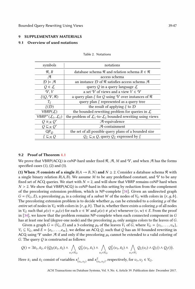
BoundedQuery Rewriting Using Views 39:47
9 SUPPLEMENTARY MATERIALS9.1 Overview of used notations
Table 2. Notations
symbols notations
R, R database schema R and relation schema R ∈ R
A access schema
D |= A an instance D of R satisfies access schema A
Q ∈ L query Q in a query language L
V , V a setV of views and a view V ∈ V
ξ (Q,V,R) a query plan ξ for Q usingV over instances of R
Tξ query plan ξ represented as a query tree
ξ (D) the result of applying ξ to D
VBRP(L) the bounded rewriting problem for queries in L
VBRP+(L1,L2) the problem of L1-to-L2 bounded rewriting using views
Q ≡A Q ′ A-equivalence
Q ⊑A Q ′ A-containment
QPQ the set of all possible query plans of a bounded size
ξ ⊑A Q Qξ ⊑A Q , query Qξ expressed by ξ
9.2 Proof of Theorem 4.1We prove that VBRP(ACQ) is coNP-hard under fixed R, A,M and V , and when A has the forms
specified cases (1), (2) and (3).
(1) When A consists of a single R(A → B,N ) and N ≥ 2. Consider a database schema R with
a single binary relation R(A,B). We assume M to be any predefined constant, and V to be any
fixed set of ACQ queries. We start with N = 2, and will show that VBRP remains coNP hard when
N > 2. We show that VBRP(ACQ) is coNP-hard in this setting by reduction from the complement
of the precoloring extension problem, which is NP-complete [34]. Given an undirected graph
G = (VG ,E), a precoloring µ0 is a coloring of a subsetW of the nodes of VG with colors in {r ,д,b}.The precoloring extension problem is to decide whether µ0 can be extended to a coloring µ of theentire set of nodes inVG with colors in {r ,д,b}. That is, whether there exists a coloring µ of all nodesin VG such that µ(v) = µ0(v) for each v ∈W and µ(v) , µ(w) whenever (v,w) ∈ E. From the proof
in [34], we know that the problem remains NP-complete when each connected component in Ghas at least one leaf (degree-one node) and the precoloring µ0 only assigns colors to the leaves ofG .Given a graph G = (VG ,E) and a 3-coloring µ0 of the leaves V1 of G, where VG = {v1, . . . ,vn},
V1 ⊆ VG , and E = {e1, . . . , em}, we define an ACQ Q , such that Q has anM-bounded rewriting in
ACQ using V under A if and only if the precoloring µ0 cannot be extended to a valid coloring of
G. The query Q is constructed as follows:
Q() = ∃x1, x2, v(QE (x1, x2) ∧
∧vi ∈VG
Q1
V (vi , x1) ∧∧
vi ∈VG
Q2
V (vi , x2) ∧∧vi ∈V1
QL(vi ) ∧Q1() ∧Qf ()).
Here x1 and x2 consist of variables x1
(vi ,vj )and x2
(vi ,vj ), respectively, for vi ,vj ∈ VG .
ACM Transactions on Database Systems, Vol. 9, No. 4, Article 39. Publication date: December 2017.

39:48 Yang Cao, Wenfei Fan, Floris Geerts, and Ping Lu
Intuitively, QE , Q1
V and Q2
V encode graphG , QL(vi ) enforces the precoloring, Q1 checks whether
G is 3-colored, andQf controlsM , as will be elaborated shortly. The challenge arises from encoding
a cyclic graph G in ACQ . We approach this as follows. We first replace two vertices of any edge in
G with two distinct new variables, and then use the fixed access constraint to recover the originalG .For example, a cycle (v1,v2), (v2,v3), (v3,v1) inG is represented by the following set of atoms inQE :
R(x1
(v1,v2),x2
(v1,v2)), R(x1
(v2,v3),x2
(v2,v3)) and R(x1
(v3,v1),x2
(v3,v1)), where x1
(v1,v2)∈ x1 and x2
(v1,v2)∈ x2;
similarly for the other variables. Although these seem like disconnected edges, we will ensure that
v1 = x1
(v1,v2)= x2
(v3,v1), v2 = x2
(v1,v2)= x1
(v2,v3)and v3 = x2
(v2,v3)= x1
(v3,v1)by means of the access
constraint and queries Q1
V and Q2
V . This allows us to recover the cycle in G, and encode cyclic
graphs in an acyclic CQ query.
We will use relation R to encode edges in E as well as coloring of vertices in VG .Queries QE ,Q
1
V ,Q2
V ,QL,Q1 and Qf are in ACQ , and are given as follows.
− The following sub-query renames the nodes of each edge in G.
QE (x1, x2) =∧
(vi ,vj )∈E
(R(x1
(vi ,vj ),x2
(vi ,vj )) ∧ R(x2
(vi ,vj ),x1
(vi ,vj ))).
We use two directed edges to encode one edge inG so that the access constraint R(A → B, 2)can be used to recover variables x1
(vi ,vj )and x2
(vi ,vj ).
− The following sub-query ensures that each variable x1
ej = x1
(vi ,vj )in x1 denotes node vi by
enforcing that x1
ej = vi .
Q1
V (vi , x1) =∧
ej=(vi ,vj )∈E
((R(i, 1) ∧ R(i,vi ) ∧ R(i,x1
ej )︸ ︷︷ ︸Qe1
j
) ∧
(R(i + n, 2) ∧ R(i + n,vi ) ∧ R(i + n,x1
ej )︸ ︷︷ ︸Qe2
j
(R(i + 2 ∗ n, 3) ∧ R(i + 2 ∗ n,vi ) ∧ R(i + 2 ∗ n,x1
ej )︸ ︷︷ ︸Qe3
j
)).
Indeed, suppose that x1
ej , vi . Then by the access constraint R(A → B, 2) ∈ A, from Qe1
j
(marked underlying Q1
V ) we know that vi = 1 ∨ x1
ej = 1. Similarly, vi = 2 ∨ x1
ej = 2 or
vi = 3 ∨ x1
ej = 3 by Qe2
jand Qe3
j. That is, {vi ,x
1
ej } = {1, 2, 3}, a contradiction. Hence x1
ej = vi .
− Similarly, the following sub-query ensures that each variable x2
ej in x2 corresponding to visatisfies x2
ej = vi .
Q2
V (vi , x2) =∧
ej=(vj ,vi )∈E
((R(i, 1) ∧ R(i,vi ) ∧ R(i,x2
ej )︸ ︷︷ ︸Qe1
j
) ∧
(R(i + n, 2) ∧ R(i + n,vi ) ∧ R(i + n,x2
ej )︸ ︷︷ ︸Qe2
j
) ∧ (R(i + 2 ∗ n, 3) ∧ R(i + 2 ∗ n,vi ) ∧ R(i + 2 ∗ n,x2
ej )︸ ︷︷ ︸Qe3
j
)).
− The following sub-query ensures that for each vertex v ∈ V1, v = µ0(v), i.e., the coloringpreserves the precoloring µ0 of the leaves, making use of R to encode the coloring.
ACM Transactions on Database Systems, Vol. 9, No. 4, Article 39. Publication date: December 2017.

BoundedQuery Rewriting Using Views 39:49
QL(vi ) = (R(i, 1) ∧ R(i,vi ) ∧ R(i, µ0(vi ))︸ ︷︷ ︸Q1
vi
) ∧ (R(i + n, 2) ∧ R(i + n,vi ) ∧ R(i + n, µ0(vi ))︸ ︷︷ ︸Q2
vi
)
∧ (R(i + 2 ∗ n, 3) ∧ R(i + 2 ∗ n,vi ) ∧ R(i + 2 ∗ n, µ0(vi ))︸ ︷︷ ︸Q3
vi
).
− The following sub-query is to ensure that graph G is colored with {r ,д,b}. Q1() = R(r ,д) ∧R(r ,b) ∧ R(д, r ) ∧ R(д,b) ∧ R(b, r ) ∧ R(b,д). More specifically, consider any instance D |= A
of R such that Q(D) , ∅. Suppose that ν is a valuation of the variables of Q to vertices in
D. We next show that for each vertex v ∈ VG , ν (v) ∈ {r ,д,b}, i.e., G is colored with {r ,д,b},and for any edge (v,v ′) ∈ E, µ(v) , µ(v ′). Let v be any vertex in VG . Since we assume that
each connected component of G has at least one leaf and each edge of G is represented by
two directed edges in GE , there exist a leaf v1 ∈ V1 and a path v1,v′1,v ′
2, . . . ,v ′
t ,v from v1
to v . Hence, there exist tuples R(ν (v1),ν (v′1)),R(ν (v ′
1),ν (v ′
2)), . . . ,R(ν (v ′
t ),ν (v)) in D. Sincev1 is a leaf, we know that v1 = µ0(v1) and ν (v1) ∈ {r ,д,b}. Suppose w.l.o.g. that ν (v1) = r .Since Q1(D) , ∅, there exist two tuples R(r ,д) and R(r ,b) in D. By the access constraint
R(A → B, 2), we have that ν (v ′1) ∈ {д,b}. Similarly, we can show that ν (v) ∈ {r ,д,b} and
hence the coloring is valid (see details below).
− Finally, we consider sub-query Qf () = ∃Y ( ∧i≤(M×|V |×|R |)
R(yi , i)). It is to fill Q with M ×
|V| × |R| constants. Since there are already another three constants r , д, and b in Q , if Q is
satisfiable, then each element query ofQ contains at leastM×|V|×|R|+3 constants. However,
eachM-bounded rewriting can only have at mostM × |V| × |R| constants. Indeed, such an
M-bounded rewriting can have at mostM × |V| atoms, and thus has at mostM × |V| × |R|
distinct constants. Therefore, Q has an M-bounded rewriting in ACQ usingV under A if
and only if Q ≡A ∅.
Obviously, Q is an ACQ . By the definition of Qf , we can see that Q has anM-bounded rewriting
in ACQ using V under A if and only if Q ≡A ∅. Thus it suffices to show that Q ≡A ∅ if and only
if the precoloring µ0 cannot be extended to a valid coloring of G.
(⇐) Suppose that µ0 cannot be extended to a valid coloring ofG . We show thatQ ≡A ∅ by contradic-
tion. Suppose thatQ .A ∅. Then there existsD |= A such thatQ(D) , ∅. Let ν be a valuation of vari-ables inQ . Clearly,QE (D) , ∅,QL(D) , ∅, andQ1(D) , ∅. FromQL(D) , ∅, we know that for each
leaf v ∈ V1, ν (v) = µ0(v). Since Q1(D) , ∅, there are tuples R(r ,д),R(r ,b),R(д, r ),R(д,b),R(b, r ),R(b,д) in D. Putting these together, by the argument about Q1 we can conclude that G is colored
with {r ,д,b}. Since QE (D) , ∅ and R(A → B, 2), for every edge (vi ,vj ) ∈ E, ν (vi ) , ν (vj ). Indeed,suppose otherwise that ν (vi ) = ν (vj ) = r , then there will be a tuple R(r , r ) in D. Now there are
three tuples R(r ,д),R(r ,b) and R(r , r ) in D, contradicting that D |= A. Therefore, there exists a
valid 3-coloring of G extending µ0, a contradiction. Hence Q ≡A ∅.
(⇒) Suppose that Q ≡A ∅. We show that µ0 cannot be extended to a valid coloring of G. Supposeby contradiction that µ is a valid 3-coloring of G that extends the precoloring µ0. We construct
below an instance D of R such that D |= A and Q(D) , ∅, which will contradict to that Q ≡A ∅.
The database D consists of the following tuples.
(1) The 6 tuples demanded by Q1: R(r ,д),R(r ,b),R(д, r ),R(д,b),R(b, r ),R(b,д).(2) For each vertex vi ∈ VG , 6 tuples corresponding to the queries Q1
V and Q2
V :
R(i, 1),R(i + n, 2),R(i + 2n, 3),R(i, µ(vi )),R(i + n, µ(vi )),R(i + 2n, µ(vi )).
ACM Transactions on Database Systems, Vol. 9, No. 4, Article 39. Publication date: December 2017.

39:50 Yang Cao, Wenfei Fan, Floris Geerts, and Ping Lu
(3) For each natural number i ≤ (M × |V| × |R|), one tuple R(ci , i), where ci ’s are distinct newconstants.
It is easy to verify that D |= A. We next show that Q(D) , ∅. Since Q1
V and Q2
V ensure that each
variable in x1 or x2 equals the corresponding variable in VG , we know that Q can be simplified to
the following query:
Q2() = ∃v (Q ′E (v) ∧
∧vi ∈VG
Q ′V (vi ) ∧
∧vi ∈VG
Q ′′V (vi ) ∧
∧vi ∈V1
QL(vi ) ∧Q1() ∧Qf ()).
Here QL,Q1() and Qf are sub-queries Q , and Q ′E , Q
′V , and Q
′′V are defined as follows:
− Q ′E (v) =
∧(vi ,vj )∈E
(R(vi ,vj ) ∧ R(vj ,vi )
);
− Q ′V (vi ) =
∧ej=(vi ,vj )∈E
((R(i, 1) ∧ R(i,vi )︸ ︷︷ ︸
Qe1
j
) ∧ (R(i + n, 2) ∧ R(i + n,vi )︸ ︷︷ ︸Qe2
j
)
∧ (R(i + 2 ∗ n, 3) ∧ R(i + 2 ∗ n,vi )︸ ︷︷ ︸Qe3
j
));
− Q ′′V (vi ) =
∧ej=(vj ,vi )∈E
((R(i, 1) ∧ R(i,vi )︸ ︷︷ ︸
Qe1
j
) ∧ (R(i + n, 2) ∧ R(i + n,vi )︸ ︷︷ ︸Qe2
j
)
∧ (R(i + 2 ∗ n, 3) ∧ R(i + 2 ∗ n,vi )︸ ︷︷ ︸Qe3
j
)).
Since Q2 is obtained from Q by simply replacing equivalent variables in Q , Q2 ≡A Q . Since thevariables in Q2 occur in either v or Y (Y is used in Qf ), we can construct a valuation ν of variables
of Q2 as follows: for each i ≤ (M × |V| × |R|), ν (yi ) = ci ; and for each vertex v ∈ VG , ν (v) = µ(v).One can verify that ν satisfies ν (Q2) ⊆ D and henceQ .A ∅, contradictingQ ≡A ∅. Thus µ0 cannot
be extended to a valid coloring of G.When N > 2, we only need to fill the relation R with some constants and use the same reduction.
For example, when N = 3, let c1, c2 and c3 be distinct new constants. Then Q1 can be rewritten
as Q1() = R(r ,д) ∧ R(r ,b) ∧ R(д, r ) ∧ R(д,b) ∧ R(b, r ) ∧ R(b,д) ∧ R(r , c1) ∧ R(д, c2) ∧ R(b, c3). This
revised Q1 also ensures that G is colored by {r ,д,b}. Indeed, consider any D |= A such that
Q(D) , ∅. Suppose that ν is a valuation of variables of Q . We show that for each vertex v ∈ VG ,ν (v) ∈ {r ,д,b}. Let v be any vertex in VG . Similar to the argument above, we can show that
there exist a leaf v1 ∈ V1 and a path v1,v′1,v ′
2, . . . ,v ′
t ,v from v1 to v . Hence, there exist tuplesR(ν (v1),ν (v
′1)),R(ν (v ′
1),ν (v ′
2)), . . . ,R(ν (v ′
t ),ν (v)) inD. Becausev1 is a leaf, we know thatv1 = µ0(v1)
and ν (v1) ∈ {r ,д,b}. Suppose that ν (v1) = r . Since Q1(D) , ∅, there are three tuples R(r ,д), R(r ,b),and R(r , c1) in D. By constraint R(A → B, 3), we have that ν (v ′
1) ∈ {д,b, c1}. However, by the
construction of QE , tuple R(ν (v′1),ν (v1)) is also in D. Hence, ν (v ′
1) also appears in the first column
of R. But c1 only appears in the second column of R. Hence ν (v ′1) , c1 and ν (v
′1) ∈ {д,b}. Using the
same argument, we can show that ν (v) ∈ {r ,д,b}. The other queries can be revised similarly. For
other values of N , we can verify the coNP hardness along the same lines.
(2) WhenA consists of two access constraints R(A → B, 1) and R′(∅ → (E, F ),N ), and N ≥ 6.
We will only use the binary relations R(A,B) and R′(E, F ) in our proof. We take any predefined
constant asM , andV to be any fixed set of ACQ queries.
We start with N = 6 and then extend the proof to N > 6. We show that VBRP(ACQ) is
coNP-hard in this setting by reduction from the complement of the 3-Colorability problem, which
ACM Transactions on Database Systems, Vol. 9, No. 4, Article 39. Publication date: December 2017.

BoundedQuery Rewriting Using Views 39:51
is NP-complete (cf. [27]). The 3-Colorability problem is to decide, given an undirected graph
G = (VG ,E), whether there exists a 3-coloring µ : VG → {r ,д,b} such that for every edge (vi ,vj ) ∈ E,µ(vi ) , µ(vj ).Given G = (VG ,E) with VG = {v1, . . . ,vn}, we define an ACQ Q such that Q has anM-bounded
rewriting in ACQ usingV under A if and only if G is not 3-colorable:
Q() = ∃v, x1, x2
(QE (x1, x2) ∧QV (v, x1, x2) ∧Q1() ∧Qf ()
).
Here QE ,QV ,Q1, and Qf are similar to their counterparts in case (1), as follows:
− QE (x1, x2) =∧
(vi ,vj )∈E
(R′(x1
(vi ,vj ),x2
(vi ,vj )) ∧ R′(x2
(vi ,vj ),x1
(vi ,vj ))), where x1
(vi ,vj )∈ x1 and
x2
(vi ,vj )∈ x2. It renames the nodes of each edge in G as in case (1).
− QV (v, x1, x2) =∧
vi ∈VG
(R(i,vi ) ∧
∧(vi ,v2)∈E
R(i,x1
(vi ,v2)) ∧
∧(v1,vi )∈E
R(i,x2
(v1,vi ))). It is to recover
the original G. Indeed, constraint R(A → B, 1) ensures that the variables vi , x1
(vi ,v2)and
x2
(v2,vi )are “equivalent”, i.e., they always take the same value.
− We define Q1() = R′(r ,д) ∧ R′(r ,b) ∧ R′(д, r ) ∧ R′(д,b) ∧ R′(b, r ) ∧ R′(b,д). Since R′(∅ →
(E, F ), 6) ∈ A, Q1 ensures that if Q() is satisfiable, then there exists a valid 3-coloring of
G. Consider any D |= A such that Q(D) , ∅, and let ν be a valuation of variables of Qin D. Then QE (D) , ∅, QV (D) , ∅, and Q1(D) , ∅. From QE (D) , ∅, we know that for
each edge (vi ,vj ) ∈ E, there exists a tuple R′(ν (x1
(vi ,vj )),ν (x2
(vi ,vj )) in D. By QV (D) , ∅ and
constraint R(A → B, 1), we have that ν (vi ) = ν (x1
(vi ,vj )) and ν (vj ) = ν (x
2
(vi ,vj )). Hence, there
exists a tuple R′(ν (vi ),ν (vj )) in D. On the other hand, since Q1(D) , ∅, there are six tuples
R′(r ,д),R′(r ,b),R′(д, r ),R′(д,b),R′(b, r ),R′(b,д) in D. By R′(∅ → (E, F ), 6) ∈ A, for each
vertex v ∈ VG , ν (v) ∈ {r ,д,b}, and for each edge (vi ,vj ) ∈ E, ν (vi ) , ν (vj ). Indeed, therelation R′
must otherwise have more than six tuples and D |= A does not hold. Therefore,
if Q() is satisfiable, then there exists a correct 3-coloring of G.− Qf () = ∃Y ∧
i≤(M×|V |×|R |)
R(yi , i). It fills Q with sufficiently many constants such that if Q is
satisfiable, then Q does not have anM-bounded rewriting in ACQ .
It can be verified that Q is in ACQ along the same lines as in case (1).
From the definition of Qf , we can conclude that Q has anM-bounded rewriting in ACQ using
V under A if and only if Q ≡A ∅. Indeed, from the argument above, we can see that if Q .A ∅,
then G is 3-colorable. Hence we only need to show that if Q ≡A ∅, then G is not 3-colorable. We
show this by contradiction. Let µ be a valid 3-coloring of G. We construct a database D such that
D |= A and Q(D) , ∅, which contradict to the assumption that Q ≡A ∅. The database D consists
of the following tuples:
(1) the 6 tuples in Q1: R′(r ,д),R′(r ,b),R′(д, r ),R′(д,b),R′(b, r ),R′(b,д);
(2) for each vertex vi ∈ VG , one tuple encoding the 3-coloring of G: R(i, µ(vi )); and(3) for each natural number i ≤ (M × |V| × |R|), one tuple R(ci , i), where ci ’s are distinct new
constants.
It is easy to verify that D |= A. We next show that Q(D) , ∅. Since QV ensures that each
variable in X 1or X 2
is equal to the corresponding variable inVG , we know thatQ can be simplified
to the following query:
Q2() = ∃v (Q ′E (v) ∧Q ′
V (v) ∧Q1() ∧Qc ()).
Here Q1() and Qc are the queries already defined in Q , and Q ′E , and Q
′V are defined as:
ACM Transactions on Database Systems, Vol. 9, No. 4, Article 39. Publication date: December 2017.
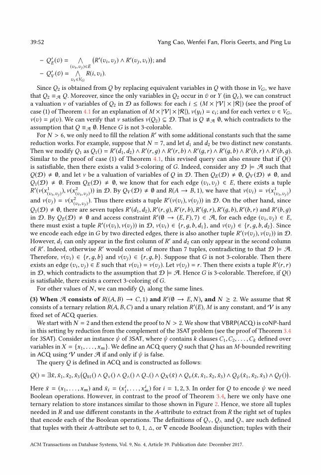
39:52 Yang Cao, Wenfei Fan, Floris Geerts, and Ping Lu
− Q ′E (v) =
∧(vi ,vj )∈E
(R′(vi ,vj ) ∧ R′(vj ,vi )
); and
− Q ′V (v) =
∧vi ∈VG
R(i,vi ).
Since Q2 is obtained from Q by replacing equivalent variables in Q with those in VG , we havethat Q2 ≡A Q . Moreover, since the only variables in Q2 occur in v or Y (in Qc ), we can construct
a valuation ν of variables of Q2 in D as follows: for each i ≤ (M × |V| × |R|) (see the proof of
case (1) of Theorem 4.1 for an explanation ofM × |V| × |R|), ν (yi ) = ci ; and for each vertex v ∈ VG ,ν (v) = µ(v). We can verify that ν satisfies ν (Q2) ⊆ D. That is Q .A ∅, which contradicts to the
assumption that Q ≡A ∅. Hence G is not 3-colorable.
For N > 6, we only need to fill the relation R′with some additional constants such that the same
reduction works. For example, suppose that N = 7, and let d1 and d2 be two distinct new constants.
Then we modify Q1 as Q1() = R′(d1,d2) ∧ R′(r ,д) ∧ R′(r ,b) ∧ R′(д, r ) ∧ R′(д,b) ∧ R′(b, r ) ∧ R′(b,д).Similar to the proof of case (1) of Theorem 4.1, this revised query can also ensure that if Q()is satisfiable, then there exists a valid 3-coloring of G. Indeed, consider any D |= A such that
Q(D) , ∅, and let ν be a valuation of variables of Q in D. Then QE (D) , ∅, QV (D) , ∅, and
Q1(D) , ∅. From QE (D) , ∅, we know that for each edge (vi ,vj ) ∈ E, there exists a tuple
R′(ν (x1
(vi ,vj )),ν (x2
(vi ,vj ))) in D. By QV (D) , ∅ and R(A → B, 1), we have that ν (vi ) = ν (x
1
(vi ,vj ))
and ν (vj ) = ν (x2
(vi ,vj )). Thus there exists a tuple R′(ν (vi ),ν (vj )) in D. On the other hand, since
Q1(D) , ∅, there are seven tuples R′(d1,d2),R′(r ,д),R′(r ,b),R′(д, r ),R′(д,b),R′(b, r ) and R′(b,д)
in D. By QE (D) , ∅ and access constraint R′(∅ → (E, F ), 7) ∈ A, for each edge (vi ,vj ) ∈ E,there must exist a tuple R′(ν (vi ),ν (vj )) in D, ν (vi ) ∈ {r ,д,b,d1}, and ν (vj ) ∈ {r ,д,b,d2}. Since
we encode each edge in G by two directed edges, there is also another tuple R′(ν (vj ),ν (vi )) in D.
However, d1 can only appear in the first column of R′and d2 can only appear in the second column
of R′. Indeed, otherwise R′
would consist of more than 7 tuples, contradicting to that D |= A.
Therefore, ν (vi ) ∈ {r ,д,b} and ν (vj ) ∈ {r ,д,b}. Suppose that G is not 3-colorable. Then there
exists an edge (vi ,vj ) ∈ E such that ν (vi ) = ν (vj ). Let ν (vj ) = r . Then there exists a tuple R′(r , r )in D, which contradicts to the assumption that D |= A. Hence G is 3-colorable. Therefore, if Q()is satisfiable, there exists a correct 3-coloring of G.For other values of N , we can modify Q1 along the same lines.
(3) When A consists of R((A,B) → C, 1) and R′(∅ → E,N ), and N ≥ 2. We assume that R
consists of a ternary relation R(A,B,C) and a unary relation R′(E),M is any constant, andV is any
fixed set of ACQ queries.
We start withN = 2 and then extend the proof toN > 2. We show that VBRP(ACQ) is coNP-hardin this setting by reduction from the complement of the 3SAT problem (see the proof of Theorem 3.4
for 3SAT). Consider an instanceψ of 3SAT, whereψ contains k clauses C1,C2, . . . ,Ck defined over
variables inX = {x1, . . . ,xm}. We define an ACQ queryQ such thatQ has anM-bounded rewriting
in ACQ usingV under A if and only ifψ is false.The query Q is defined in ACQ and is constructed as follows:
Q() = ∃x , x1, x2, x3
(Q01() ∧Q∨() ∧Q∧() ∧Q¬() ∧QX (x) ∧Qv (x , x1, x2, x3) ∧Qψ (x1, x2, x3) ∧Qf ()
).
Here x = (x1, . . . ,xm) and xi = (x i1, . . . ,x im) for i = 1, 2, 3. In order for Q to encode ψ we need
Boolean operations. However, in contrast to the proof of Theorem 3.4, here we only have one
ternary relation to store instances similar to those shown in Figure 2. Hence, we store all tuples
needed in R and use different constants in the A-attribute to extract from R the right set of tuples
that encode each of the Boolean operations. The definitions of Q∨, Q∧ and Q¬ are such defined
that tuples with their A-attribute set to 0, 1, △, or ∇ encode Boolean disjunction; tuples with their
ACM Transactions on Database Systems, Vol. 9, No. 4, Article 39. Publication date: December 2017.

BoundedQuery Rewriting Using Views 39:53
A-attribute set to ⊥ or ⊤ encode Boolean conjunction; and tuples with their A-attribute set to ⋆encode Boolean negation. More specifically, Q∧,Q∨, and Q¬ are defined as follows:
- Q∨() =(R(0, 0,△)∧R(0, 1,∇)∧R(1, 0,∇)∧R(1, 1,∇)
)∧(R(△, 0,⊥)∧R(△, 1,⊤)∧R(∇, 0,⊤)∧
R(∇, 1,⊤));
- Q∧() = R(⊥,⊥,⊥) ∧ R(⊥,⊤,⊥) ∧ R(⊤,⊥,⊥) ∧ R(⊤,⊤,⊤);- Q¬() = R(⋆, 0, 1) ∧ R(⋆, 1, 0); and
where ∇,△,⊥,⊤ and ⋆ are new constants. The constants △,⊥ and ∇,⊤ represent false and true,respectively. Sub-queries Q01 and QX are defined as follows:
- Q01() = R′(0) ∧ R′(1) ∧ R(▶, 0, 0) ∧ R(▶, 1, 1) is used to encode the Boolean values false and
true; here ▶ is a new constant; and
- QX (x) =∧
1≤i≤m(R′(xi ) ∧ R(▶,xi ,xi )) ensures that x is a truth assignment of X . Indeed,
constraint R′(∅ → E, 2) together with Q01 ensures that each xi is mapped to {0, 1} when QXis evaluated on instances D such that D |= A and Q01(D) , ∅.
It should be remarked that even without using the relation R, Q01() and QX (x) can also ensure that
x is a truth assignment of X . However, we will use these atoms to handle the cases when N > 2, as
will become clear shortly.
Furthermore, Qv ,Qψ and Qf are defined as follows:
- Qv (x , x1, x2, x3) =( ∧
1≤i≤mR(i + 2, •,xi )
)∧( ∧
1≤i≤kR(f1(Ci ) + 2, •,x1
i ) ∧ R(f2(Ci ) + 2, •,x2
i ) ∧
R(f3(Ci ) + 2, •,x3
i )), where • is a new constant and for j = 1, 2, 3, fj (Ci ) = ℓ if xℓ is the jth
variable in clause Ci .
This query is used to rename the variables in x such that each clause has a new copy of
the variables in x , represented by x1, x2, and x3, one copy for each of the three literals in
a clause. Moreover, if fj (Ci ) = ℓ then x ji and xℓ are equivalent due to access constraint
R((A,B) → C, 1), i.e., these variables take the same values in instances D |= A of R. This
allows us to encodeψ by using distinct variables to ensure acyclicity, as will be elaborated
shortly.
- Query Qψ (x1, x2, x3) is to check whetherψ is true given a truth assignment µX encoded in
x (and thus also in x1, x2, x3 since they carry the same values as x) by query Qv . We first
explain how clauses Cj in ψ are encoded. Consider, e.g., Cj = x1 ∨ x2 ∨ x3. We construct a
query Q j (x1, x2, x3,yj ) such that yj holds the truth value of Cj given µX . More specifically,
Q j (x2, x2, x3,yj ) = ∃x ′2,y ′ R(x1
j ,x′2,y ′) ∧ R(y ′,x3
j ,yj ) ∧ R(⋆,x2
j ,x′2). Note that x1
j , x2
j and x3
jtake Boolean values as specified by x1, x2 and x3, respectively, as argued earlier. Hence, by
the definitions of Q∨ and Q¬, Q j correctly encodes Cj . Moreover, observe that yj is either ⊥(when Cj is false under µX ) or ⊤ (when Cj is true under µX ). In the context of acyclicity, it is
also important to observe that the variables x1
j , x2
j and x3
j are only used in Q j (x1, x2, x3,yj )
and in Qv (x , x1, x2, x3), where they occur together with constants. The construction of Q j is
similar for clauses of another form. We now define
Qψ (x1, x2, x3) = ∃y ( ∧1≤j≤k
Q j (x1, x2, x3,yj ))∧Q ′(y1,y2, . . . ,yk ),
where Q ′(y1,y2, . . . ,yk ) checks whether y1 ∧ y2 ∧ · · · ∧ yk evaluates to true, i.e., whetherall clauses in ψ are satisfied. In particular, Q ′(y) = ∃v R(y1,y2,v2) ∧ R(v2,y3,v3) ∧ · · · ∧
R(vk−1,yk ,⊤). Since the yi ’s take values from {⊥,⊤}, by the definition ofQ∧,Q′encodes the
required conjunction and enforces all yi ’s to be ⊤ (due to the last atom). The acyclicity of Qψ
ACM Transactions on Database Systems, Vol. 9, No. 4, Article 39. Publication date: December 2017.
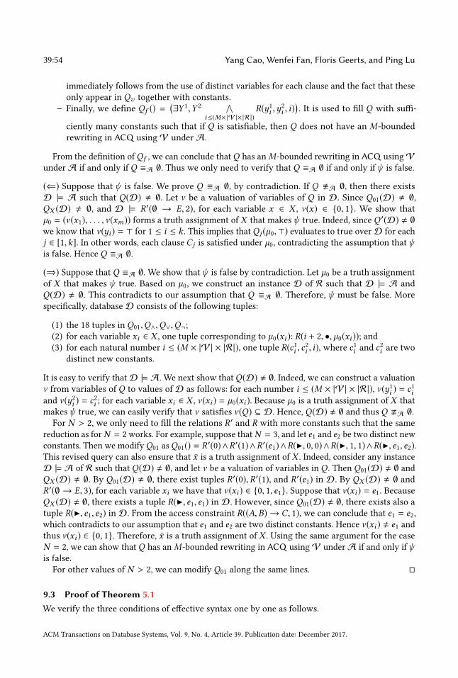
39:54 Yang Cao, Wenfei Fan, Floris Geerts, and Ping Lu
immediately follows from the use of distinct variables for each clause and the fact that these
only appear in Qv together with constants.
− Finally, we define Qf () =(∃Y 1,Y 2
∧i≤(M×|V |×|R |)
R(y1
i ,y2
i , i)). It is used to fill Q with suffi-
ciently many constants such that if Q is satisfiable, then Q does not have an M-bounded
rewriting in ACQ using V under A.
From the definition ofQf , we can conclude thatQ has anM-bounded rewriting in ACQ usingV
under A if and only if Q ≡A ∅. Thus we only need to verify that Q ≡A ∅ if and only ifψ is false.
(⇐) Suppose that ψ is false. We prove Q ≡A ∅, by contradiction. If Q .A ∅, then there exists
D |= A such that Q(D) , ∅. Let ν be a valuation of variables of Q in D. Since Q01(D) , ∅,
QX (D) , ∅, and D |= R′(∅ → E, 2), for each variable x ∈ X , ν (x) ∈ {0, 1}. We show that
µ0 = (ν (x1), . . . ,ν (xm)) forms a truth assignment of X that makesψ true. Indeed, since Q ′(D) , ∅
we know that ν (yi ) = ⊤ for 1 ≤ i ≤ k . This implies thatQ j (µ0,⊤) evaluates to true over D for each
j ∈ [1,k]. In other words, each clause Cj is satisfied under µ0, contradicting the assumption thatψis false. Hence Q ≡A ∅.
(⇒) Suppose that Q ≡A ∅. We show thatψ is false by contradiction. Let µ0 be a truth assignment
of X that makes ψ true. Based on µ0, we construct an instance D of R such that D |= A and
Q(D) , ∅. This contradicts to our assumption that Q ≡A ∅. Therefore, ψ must be false. More
specifically, database D consists of the following tuples:
(1) the 18 tuples in Q01,Q∧,Q∨,Q¬;
(2) for each variable xi ∈ X , one tuple corresponding to µ0(xi ): R(i + 2, •, µ0(xi )); and(3) for each natural number i ≤ (M × |V| × |R|), one tuple R(c1
i , c2
i , i), where c1
i and c2
i are two
distinct new constants.
It is easy to verify that D |= A. We next show thatQ(D) , ∅. Indeed, we can construct a valuation
ν from variables of Q to values of D as follows: for each number i ≤ (M × |V| × |R|), ν (y1
i ) = c1
iand ν (y2
i ) = c2
i ; for each variable xi ∈ X , ν (xi ) = µ0(xi ). Because µ0 is a truth assignment of X that
makesψ true, we can easily verify that ν satisfies ν (Q) ⊆ D. Hence, Q(D) , ∅ and thus Q .A ∅.
For N > 2, we only need to fill the relations R′and R with more constants such that the same
reduction as for N = 2 works. For example, suppose that N = 3, and let e1 and e2 be two distinct new
constants. Then we modifyQ01 asQ01() = R′(0)∧R′(1)∧R′(e1)∧R(▶, 0, 0)∧R(▶, 1, 1)∧R(▶, e1, e2).
This revised query can also ensure that x is a truth assignment of X . Indeed, consider any instance
D |= A of R such that Q(D) , ∅, and let ν be a valuation of variables in Q . Then Q01(D) , ∅ and
QX (D) , ∅. By Q01(D) , ∅, there exist tuples R′(0),R′(1), and R′(e1) in D. By QX (D) , ∅ and
R′(∅ → E, 3), for each variable xi we have that ν (xi ) ∈ {0, 1, e1}. Suppose that ν (xi ) = e1. Because
QX (D) , ∅, there exists a tuple R(▶, e1, e1) in D. However, since Q01(D) , ∅, there exists also a
tuple R(▶, e1, e2) in D. From the access constraint R((A,B) → C, 1), we can conclude that e1 = e2,
which contradicts to our assumption that e1 and e2 are two distinct constants. Hence ν (xi ) , e1 and
thus ν (xi ) ∈ {0, 1}. Therefore, x is a truth assignment of X . Using the same argument for the case
N = 2, we can show thatQ has anM-bounded rewriting in ACQ usingV under A if and only ifψis false.For other values of N > 2, we can modify Q01 along the same lines. □
9.3 Proof of Theorem 5.1We verify the three conditions of effective syntax one by one as follows.
ACM Transactions on Database Systems, Vol. 9, No. 4, Article 39. Publication date: December 2017.
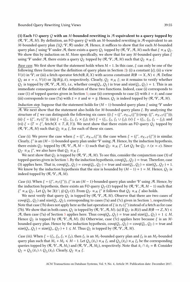
BoundedQuery Rewriting Using Views 39:55
(1) Each FO query Q with an M-bounded rewriting is A-equivalent to a query topped by(R,V,A,M). By definition, an FO query Q with anM-bounded rewriting is A-equivalent to an
M-bounded query plan ξ (Q,V,R) under A. Hence, it suffices to show that for eachM-bounded
query plan ξ usingV underA, there exists a queryQξ topped by (R,V,A,M) such that ξ ≡A Qξ .
We show this by induction onM . More specifically, we show that for anyM-bounded query plan ξusingV under A, there exists a query Qξ topped by (R,V,A,M) such that Qξ ≡A ξ .
Base case. We first show that the statement holds when M = 1. In this case, ξ can only be one of the
following three forms (see the definition of query plans in Section 2): (i) a constant {c}; (ii) a viewV (x) in V; or (iii) a fetch operator fetch(∅,R,X ) with access constraint R(∅ → X ,N ) ∈ A. Define
Qξ as x = c , V (x) or ∃y R(y, x), respectively. Clearly, Qξ ≡A ξ ; so it remains to verify whether
Qξ is topped by (R,V,A,M), i.e., whether covq(Qϵ ,Qξ ) is true and size(Qϵ ,Qξ ) = 1. This is an
immediate consequence of the definition of these two functions. Indeed, case (i) corresponds to
case (1) of topped queries given in Section 5; case (ii) corresponds to case (2) with z = x ; and case
(iii) corresponds to case (7a) with z = x and w = y. Hence, Qξ is indeed topped by (R,V,A,M).
Induction step. Suppose that the statement holds for (M − 1)-bounded query plans ξ usingV under
A. We next show that the statement also holds for M-bounded query plans ξ . By analyzing the
structure of ξ we can distinguish the following six cases: (i) ξ = (ξ ′, σX=c (ξ′)) (resp. (ξ ′, σX=Y (ξ
′)));
(ii) ξ = (ξ ′, πY (ξ′)); (iii) ξ = (ξ1, ξ2, ξ1 × ξ2); (iv) ξ = (ξ1, ξ2, ξ1 ∪ ξ2); (v) ξ = (ξ1, ξ2, ξ1 − ξ2); and
(vi) ξ = (T = ξ ′, fetch(X ∈ T ,R,Y )). We next show that there exists an FO query Qξ topped by
(R,V,A,M) such that Qξ ≡A ξ , for each of these six cases.
Case (i). We prove the case when ξ = (ξ ′, σX=c (ξ′)); the case when ξ = (ξ ′, σX=Y (ξ
′)) is similar.
Clearly, ξ ′ is an (M − 1)-bounded query plan underV usingA. Hence, by the induction hypothesis,
there exists Qξ ′ topped by (R,V,A,M − 1) such that Qξ ′ ≡A ξ ′. Let Qξ be Qξ ′ ∧ (x = c). SinceQξ ′ ≡A ξ ′, we also have that Qξ ≡A ξ .
We next show thatQξ is topped by (R,V,A,M). To see this, consider the conjunction case (3) of
topped queries given in Section 5. By the induction hypothesis, covq(Qϵ ,Qξ ′) = true. Therefore, case(3) applies here. That is, covq(Qϵ ,Qξ ) = covq(Qϵ ,Qξ ′) = true and size(Qϵ ,Qξ ) = size(Qϵ ,Qξ ′) + 1.
We know by the induction hypothesis that the size is bounded by (M − 1) + 1 = M . Hence, Qξ is
indeed topped by (R,V,A,M).
Case (ii). When ξ = (ξ ′,πY (ξ′)), ξ ′ is an (M − 1)-bounded query plan under V using A. Hence, by
the induction hypothesis, there exists an FO query Qξ ′(z) topped by (R,V,A,M − 1) such that
ξ ′ ≡A Qξ ′ . Let Qξ be ∃(z \ y)Qξ ′(z). From Qξ ′ ≡A ξ ′ it follows that Qξ ≡A ξ also holds.
We next verify that query Qξ is topped by (R,V,A,M). Observe that there are two cases of
covq(Qϵ ,Qξ ) and size(Qϵ ,Qξ ), corresponding to cases (7a) and (7c) given in Section 5, respectively.
Note that case (7b) does not apply here as the last operation of ξ is πY (ξ′) instead of a fetch as for case
(7b). We show that in both cases,Qξ is topped by (R,V,A,M). (a) IfQξ ′ is R(z) and R(∅ → Z ,N ) ∈
A, then case (7a) of Section 5 applies here. Thus covq(Qϵ ,Qξ ) = true and size(Qϵ ,Qξ ) = 1 ≤ M .
Hence Qξ is topped by (R,V,A,M). (b) Otherwise, case (7c) applies here because ξ is an M-
bounded query plan. Hence by the induction hypothesis, covq(Qϵ ,Qξ ) = covq(Qϵ ,Qξ ′) = true and
size(Qϵ ,Qξ ) = size(Qϵ ,Qξ ′) + 1 ≤ M . Thus Qξ is topped by (R,V,A,M).
Case (iii). When ξ = (ξ1, ξ2, ξ1 × ξ2), then ξ1 is anM1-bounded query plan and ξ2 is anM2-bounded
query plan such thatM1 +M2 ⩽ M − 1. LetQξ1(x1) ≡A ξ1 andQξ2
(x2) ≡A ξ2 be the corresponding
queries topped by (R,V,A,M1) and (R,V,A,M2), respectively. Note that x1 ∩ x2 = ∅. Consider
Qξ = Qξ1(x1) ∧Qξ2
(x2). Clearly, Qξ ≡A ξ .
ACM Transactions on Database Systems, Vol. 9, No. 4, Article 39. Publication date: December 2017.

39:56 Yang Cao, Wenfei Fan, Floris Geerts, and Ping Lu
We show that query Qξ is topped by (R,V,A,M). Since covq(Qϵ ,Qξ1) and covq(Qϵ ,Qξ2
) are
both true, we know from the conjunction case (4b) of topped queries given in Section 5 that
covq(Qϵ ,Qξ ) = true as well. Furthermore, since x1 ∩ x2 = ∅, size(Qϵ ,Qξ ) is defined in case (4b) as
2 · size(Qϵ ,Qϵ )+ size(Qϵ ,Qξ1)+ size(Qϵ ,Qξ2
)+ 1, which is bounded byM1 +M2 + 1 ⩽ M . Therefore,
query Qξ is topped by (R,V,A,M).
Case (iv). The case when ξ = (ξ1, ξ2, ξ1 ∪ ξ2) is verified in the same way as the previous case, by
using the disjunction case (5) of topped queries specified in Section 5.
Case (v). When ξ = (ξ1, ξ2, ξ1 \ ξ2), the case is handled in the same way as case (iii), by using the
negation case (6a) given in Section 5.
Case (vi). When ξ = (S = ξ ′, fetch(X ∈ S,R,Z )), since ξ is an M-bounded query plan using V
under A, we know that there exists an access constraint R(X → Z ′,N ) in A such that Z ⊆ X ∪Z ′
and as before, ξ ′ is an (M − 1)-bounded query plan usingV under A. In addition, ξ ′ must have
bounded output. Hence, the induction hypothesis applies here. Let Qξ ′(x) be a query topped by
(R,V,A,M − 1) such that Qξ ′(x) ≡A ξ ′ and consider Qξ (x , z) = Qξ ′(x) ∧ ∃u R(x , z, u). Clearly,Qξ (x , z) ≡A ξ .
We next verify that query Qξ is topped by (R,V,A,M). This follows from the conjunction case
(4a) given in Section 5. Indeed, by the induction hypothesis we have that covq(Qϵ ,Qξ ′) = true.Furthermore, Qξ ′(x) has bounded output. Thus by the definition of topped queries in case 4(a), we
have that covq(Qϵ ,Qξ ) = true and size(Qϵ ,Qξ ) = size(Qϵ ,Qξ ′) + 1 bounded by M . Hence Qξ is
topped by (R,V,A,M).
(2) Every query topped by (R,V,A,M) has anM-bounded rewriting usingV underA. We
show that every queryQ topped by (R,V,A,M) indeed has a size(Qϵ ,Q)-bounded rewriting usingV under A. The statement we will prove is as follows:
if covq(Qϵ ,Qs ) = covq(Qs ,Q) = true and Qs has a size(Qϵ ,Qs )-bounded plan, thencovq(Qϵ ,Qs ∧Q) = true and Qs ∧Q has a size(Qϵ ,Qs ∧Q)-bounded plan.
For if this holds, then Q has anM-bounded plan if it is topped by (R,V,A,M). Indeed, when
Q is topped by (R,V,A,M), covq(Qϵ ,Q) = true and size(Qϵ ,Q) ≤ M . Since covq(Qϵ ,Qϵ ) = trueand Qϵ has a 0-bounded plan, by the statement, Qϵ ∧Q = Q has a size(Qϵ ,Qϵ ∧Q) = size(Qϵ ,Q)-bounded plan, i.e., anM-bounded plan. That is,Q has anM-bounded rewriting usingV under A if
Q is topped by (R,V,A,M).
Below we prove the statement by induction on the structure of Q . In the sequel, for a tuple x of
variable, we denote by X its corresponding set of attributes, and vice versa.
Base case. We first show that the statement holds whenQ has one of the following forms: (b1) z = c ;(b2) a view V (z) inV; or (b3) a relation ∃w R(w, z).
Case (b1). For base case (b1), i.e., when Q is z = c , if covq(Qϵ ,Qs ) = covq(Qs ,Q) = true and Qs has
a size(Qϵ ,Qs )-bounded plan (say ξs ), then consider plan ξ = (ξs , σz=c (ξs )). SinceQs ≡A ξs , we havethat Qs ∧ Q ≡A ξ . Since covq(Qs ,Q) = true, we know that case (3) of topped queries specified
in Section 5 can apply to Qs ∧Q . Hence covq(Qϵ ,Qs ∧Q) = covq(Qϵ ,Qs ) = true and Qs ∧Q has
a (|ξs | + 1)-bounded plan, where |ξs | + 1 ≤ size(Qϵ ,Qs ) + 1 = size(Qϵ ,Qs ∧ (z = c)). That is, thestatement holds for case (b1).
Case (b2). For base case (b2), i.e., when Q is a view V (z), if covq(Qϵ ,Qs ) = covq(Qs ,Q) = true and
Qs has a size(Qϵ ,Qs )-bounded plan (say ξs ), then we have the following plans for Qs ∧ Q . ForQs (x) and V (z), (i) if x ∩ z = ∅, then let plan ξ be (T1 = ξs , T2 = V (z), T3 = T1 × T2); and (ii) if
ACM Transactions on Database Systems, Vol. 9, No. 4, Article 39. Publication date: December 2017.

BoundedQuery Rewriting Using Views 39:57
x ∩ z = w , ∅, then let plan ξ be (T1 = ξs ,T2 = V (z),T3 = ρ(T2),T4 = T1 ×T3,T5 = σT1[W ]=T3[W ](T4),
T6 = πT1[X ],T3[Z \W ](T5)). In both cases, ξ ≡A Qs ∧Q when ξs ≡A Qs . Moreover, note that by case
(2) of Section 5 we have that covq(Qϵ ,V (z)) = true, since covq(Qϵ ,Qs ) = true following case (4b)
of Section 5 we also have that covq(Qϵ ,Qs ∧V (z)) = true and size(Qϵ ,Qs ∧V (z)) = size(Qϵ ,Qϵ ) +
size(Qϵ ,Qs ) + size(Qϵ ,V (z)) + λ(x, z) ≥ |ξ | in both cases (i) and (ii) (recall λ(x, z) from case (4b); note
that λ(x, z) = 1 for case (i) and λ(x, z) = 4 for case (ii)). Therefore, the statement holds for case (b2).
Case (b3). For base case (b3), i.e., when Q is ∃wR(w, z), if covq(Qϵ ,Qs ) = covq(Qs ,Q) = true and
Qs has a size(Qϵ ,Qs )-bounded plan ξs , observe the following. Given that covq(Qs ,Q) = true, fromcases (7a-7b) of Section 5, we know that either (i) R(∅ → Z ,N ) ∈ A or (ii) R(X → Z ′,N ) ∈ A,
X ∪ Z ′= Z and Qs (x) has bounded output under A.
First consider case (i). We distinguish two cases: x ∩ z = ∅, and x ∩ z = w ′ , ∅. When x ∩ z = ∅,
let ξ = (T1 = ξs , T2 = fetch(∅,R,Z ), T3 = T1 × T2). Since ξs ≡A Qs , we have that ξ ≡A Q .Observe that by case (7a) of Section 5, covq(Qϵ ,Q) = true. In addition, covq(Qϵ ,Qs ) = true by the
condition of the statement. Therefore, case (4b) specified in Section 5 applies to Qs ∧ Q . Hencecovq(Qϵ ,Qs ∧Q) = true, size(Qϵ ,Qs ∧Q) = size(Qϵ ,Qs ) + size(Qϵ ,Q) + 1 = size(Qϵ ,Qs ) + 2 ≥ |ξ |.That is, Qs ∧Q has a size(Qϵ ,Qs ∧Q)-bounded plan. For the case when x ∩ z = w ′ , ∅, one can
verify that Qs (x) ∧Q(z) has a size(Qϵ ,Qs ∧Q)-bounded plan along the same lines as above.
Next consider case (ii). Since Qs has bounded output under A and covq(Qϵ ,Qs ) = true, case (4a)given in Section 5 applies to covq(Qϵ ,Qs ∧ Q) here. Hence covq(Qϵ ,Qs ∧ Q) = true. Consider aplan ξ = (T1 = ξs , T2 = fetch(X ∈ T1,R,Z
′)). Since ξs ≡A Qs , we have that ξ ≡A Qs ∧ Q . Hence|ξ | = |ξs | + 1 ≤ size(Qϵ ,Qs ) + 1 = size(Qϵ ,Qs ∧Q) by case (4a) of Section 5. That is, Qs ∧Q has a
size(Qϵ ,Qs ∧Q)-bounded plan.
Induction step. Assume that the statement holds for sub-queries of a topped query Q . Below we
show that the statement also holds for Q itself, by analyzing the structure of Q(z) as follows,corresponding to the different cases presented in Section 5. We number the cases accordingly in
the proof below.
(3) Q(z) is Q ′(z) ∧ (x = c). Since covq(Qs ,Q) = true, we know that covq(Qs ,Q′) = true as well.
Since covq(Qϵ ,Qs ) = true and Qs has a size(Qϵ ,Qs )-bounded plan, by the induction hypothesis,
covq(Qϵ ,Qs∧Q′) = true andQs∧Q
′has a size(Qϵ ,Qs∧Q
′)-bounded plan ξ ′. Thus, by the definitionof covq(·, ·) in case (3) in Section 5, we know that covq(Qϵ ,Qs ∧ (Q ′ ∧ (x = c))) = true. Moreover,
Qs ∧Q has a bounded plan ξ = (T1 = ξ′, T2 = σX=cT1) and |ξ | = |ξ ′ | + 1 ≤ size(Qϵ ,Qs ∧Q ′) + 1 =
size(Qϵ ,Qs ∧Q). That is, the statement holds forQ(z). The cases whenQ isQ ′∧(x = y),Q ′∧(x , y)or Q ′ ∧ (x , c) can be verified in the same way.
(4) Q(z) is Q1(z1) ∧ Q2(z2). There are three cases (4a), (4b) and (4c) of topped queries given in
Section 5 when covq(Qs ,Q(z)) = true. We verify these cases one by one below.
Case (4a). For case (4a) of topped queries specified in Section 5, when covq(Qs ,Q) = true, wehave that covq(Qs ,Q1(z1)) = true, Q2(z2) is a relation ∃w R(z1, z
′2, w), R(Z1 → Z ′
2,N ) ∈ A with
Z1 ∪ Z ′2= Z2, and Qs ∧Q1 has bounded output under A. Now consider Qs ∧Q = Qs ∧ (Q1 ∧Q2).
Since covq(Qs ,Q1) = covq(Qϵ ,Qs ) = true andQs has a size(Qϵ ,Qs )-bounded plan, by the induction
hypothesis we know that covq(Qϵ ,Qs ∧Q1) = true and Qs ∧Q1 has a size(Qϵ ,Qs ∧Q1)-bounded
plan ξs1. In addition, ξs1 has bounded output. Now case (4c) in Section 5 applies toQs ∧ (Q1 ∧Q2) to
handle multiple conjuncts. Thus covq(Qϵ ,Qs ∧(Q1 ∧Q2)) = covq(Qϵ ,Qs )∧covq(Qs ,Q1 ∧Q2) = true.Consider plan ξ = (T1 = ξs1, T2 = fetch(T1,R,Z
′2)). Note that ξ ≡A Qs ∧Q because ξs1 ≡A Qs ∧Q1.
SinceTs1 is of bounded size, ξ is a (|ξs1 |+1)-bounded plan, where (|ξs1 |+1) ≤ size(Qϵ ,Qs ∧Q1)+1 =
ACM Transactions on Database Systems, Vol. 9, No. 4, Article 39. Publication date: December 2017.

39:58 Yang Cao, Wenfei Fan, Floris Geerts, and Ping Lu
size(Qϵ , (Qs ∧Q1) ∧Q2) ≤ size(Qϵ ,Qs ∧Q). That is, the statement holds forQ whenQ falls in case
(4a).
Case (4b). For case (4b) of topped queries of Section 5, when covq(Qs ,Q) = true, we have thatcovq(Qs ,Q1) = covq(Qs ,Q2) = true. To be more specific, we distinguish four cases: (i) covq(Qϵ ,Q1)
= covq(Qϵ ,Q2) = true, (ii) covq(Qϵ ,Q1) = true and covq(Qϵ ,Q2) = false, (iii) covq(Qϵ ,Q1) = false andcovq(Qϵ ,Q2) = true, and (iv) covq(Qϵ ,Q1) = covq(Qϵ ,Q2) = false. Assume z1 ∧ z2 = ∅. For case (i),
since covq(Qϵ ,Qi ) = true(i ∈ {1, 2}), by the induction hypothesis, there are size(Qϵ ,Qi )-bounded
plans ξi forQi . Let ξs be the size(Qϵ ,Qs )-bounded plan forQs Now consider plan ξ = (T1 = ξ1,T2 =
ξ2,T3 = T1 × T2,T4 = ξs ,T5 = T3 × T4). Then ξ ≡A ξ . Note that |ξ | = |ξ1 | + |ξ2 | + |ξs | + 2 ≤
size(Qϵ ,Q1) + size(Qϵ ,Q2) + size(Qϵ ,Qs ) + 2. Hence size(Qϵ ,Qs ∧ (Q1 ∧ Q2)) = size(Qϵ ,Qs ) +
size(Qϵ ,Q1 ∧Q2) + 1 = size(Qϵ ,Qs ) + size(Qϵ ,Q1) + size(Qϵ ,Q2) + 1 + 1 ≥ |ξ |. For case (ii), sincecovq(Qϵ ,Q1) = true and covq(Qs ,Q2) = true, by the induction hypothesis, we know that Q1 has
a size(Qϵ ,Q1)-bounded plan ξ1 and Qs ∧ Q2 has a size(Qϵ ,Qs ∧ Q2)-bounded plan ξs2 (note that
covq(Qϵ ,Qs ∧Q2) = covq(Qϵ ,Qs )∧covq(Qs ,Q2) = true). Consider plan ξ = (T1 = ξ1,T2 = ξs2,T3 =
T1 × T2). Then ξ ≡A Q1 ∧ (Qs ∧ Q2) = Qs ∧ Q and |ξ | ≤ size(Qϵ ,Q1) + size(Qϵ ,Qs ∧ Q2) + 1 =
size(Qϵ ,Q1) + size(Qϵ ,Qs ) + size(Qs ,Q2) + 1. Note that size(Qϵ ,Qs ∧ (Q1 ∧Q2)) = size(Qϵ ,Qs ) +
size(Qs ,Q1 ∧ Q2) = 3 ∗ size(Qϵ ,Qs ) + size(Qs ,Q1) + size(Qs ,Q2) + 1. In addition, one can easily
verify that, when covq(Qϵ ,Q) = covq(Qs ,Q) = true, size(Qϵ ,Q) ≤ size(Qs ,Q), by induction on Q .Hence size(Qϵ ,Qs ∧Q) ≥ |ξ |. Similarly for case (iii). For case (iv), from covq(Qϵ ,Qi ) , true and
covq(Qs ,Qi ) = true and the induction hypothesis we know that Qs ∧Qi has a size(Qϵ ,Qs ∧Qi )-
bounded plan ξsi , for i ∈ {1, 2}. Consider plan ξ = (T1 = ξs1,T2 = ξs2,T3 = T1 × T2). Then
ξ ≡A (Qs ∧Q1) ∧ (Qs ∧Q2) = Qs ∧Q . Note that |ξ | ≤ size(Qϵ ,Qs ∧Q1) + size(Qϵ ,Qs ∧Q2) + 1 =
2∗size(Qϵ ,Qs )+size(Qs ,Q1)+size(Qs ,Q2)+1. Hence size(Qϵ ,Qs ∧Q) = size(Qϵ ,Qs )+size(Qs ,Q1∧
Q2) = size(Qϵ ,Qs )+2size(Qϵ ,Qs )+size(Qs ,Q1)+size(Qs ,Q2)+1 ≥ |ξ |. Similarly, one can verify the
case when z1∩z2 , ∅. Furthermore,covq(Qϵ ,Qs∧Q) = true since covq(Qϵ ,Qs )∧covq(Qs ,Q) = true.Therefore, we have that the statement holds on Q in case (4b).
Case (4c). When Q falls in case (4c) of topped queries in Section 5, from covq(Qs ,Q1 ∧Q2) = truewe know that covq(Qϵ ,Qs ∧Q1) = true and covq(Qs ∧Q1,Q2) = true. By the induction hypothesis,
from covq(Qϵ ,Qs ∧ Q1) = true we have that Qs ∧ Q1 has a size(Qϵ ,Qs ∧ Q1)-bounded plan ξs1.
Hence, further by the induction hypothesis, from covq(Qϵ ,Qs ∧Q1) = covq(Qs ∧Q1,Q2) = true andthatQs ∧Q1 has plan ξs1, we have that (Qs ∧Q1)∧Q2 has a size(Qϵ , (Qs ∧Q1)∧Q2)-bounded plan ξ ,by treating (Qs ∧Q1) as a “newQs ”. Note that ξ is also a plan forQs ∧ (Q1 ∧Q2). Observe that |ξ | ≤size(Qϵ , (Qs∧Q1)∧Q2) = size(Qϵ ,Qs∧Q1)+size(Qs∧Q1,Q2) = size(Qϵ ,Qs )+size(Qs ,Q1)+size(Qs∧
Q1,Q2) (by case (4c)). Therefore, by case (4c) size(Qϵ ,Qs∧(Q1∧Q2)) = size(Qϵ ,Qs )+size(Qs ,Q1∧Q2)
= size(Qϵ ,Qs )+size(Qs ,Q1)+size(Qs∧Q1,Q2) ≥ |ξ |. Since covq(Qϵ ,Qs∧(Q1∧Q2)) = covq(Qϵ ,Qs )∧
covq(Qs ,Q1 ∧Q2) = true, the statement holds on Q when Q is in case (4c).
A size(Qϵ ,Qs ∧ Q)-bounded plan in this case can be constructed along the same lines as its
counterpart for (4b) above, distinguishing the case when there exist common variables in Qs ∧Q1
and Q2 from the case when they contain disjoint variables.
Remark. Note that whenQ =Q1∧Q2, to compute covq(Qs ,Q), we need to compute both covq(Qs ,Q2)
(case (4b)) and covq(Qs∧Q1,Q2) (case (4c)). WhenQ2 isQ21∧Q22, we need to compute covq(Qs ,Q22),
covq(Qs ∧Q1,Q22), covq(Qs ∧Q21, Q22) and covq(Qs ∧Q1 ∧Q21, Q22). In the worst case, we test
2|Q2 |
many different cases. Hence we restrict the size of Q2 to bound the number of expansions of
Qs when computing covq(Qϵ ,Q) to ensure that covq(·, ·) is computable in PTIME (statement (3) of
Theorem 5.1), although this has no impact on the statement we are proving now.
ACM Transactions on Database Systems, Vol. 9, No. 4, Article 39. Publication date: December 2017.
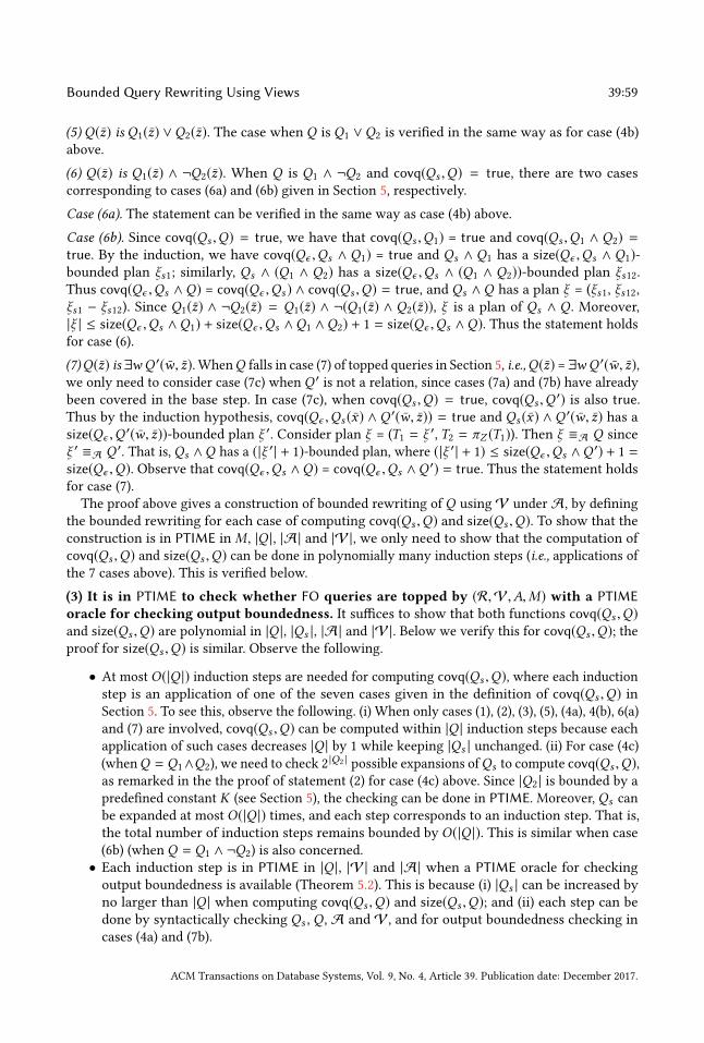
BoundedQuery Rewriting Using Views 39:59
(5) Q(z) is Q1(z) ∨Q2(z). The case when Q is Q1 ∨Q2 is verified in the same way as for case (4b)
above.
(6) Q(z) is Q1(z) ∧ ¬Q2(z). When Q is Q1 ∧ ¬Q2 and covq(Qs ,Q) = true, there are two cases
corresponding to cases (6a) and (6b) given in Section 5, respectively.
Case (6a). The statement can be verified in the same way as case (4b) above.
Case (6b). Since covq(Qs ,Q) = true, we have that covq(Qs ,Q1) = true and covq(Qs ,Q1 ∧ Q2) =
true. By the induction, we have covq(Qϵ ,Qs ∧ Q1) = true and Qs ∧ Q1 has a size(Qϵ ,Qs ∧ Q1)-
bounded plan ξs1; similarly, Qs ∧ (Q1 ∧ Q2) has a size(Qϵ ,Qs ∧ (Q1 ∧ Q2))-bounded plan ξs12.
Thus covq(Qϵ ,Qs ∧Q) = covq(Qϵ ,Qs ) ∧ covq(Qs ,Q) = true, and Qs ∧Q has a plan ξ = (ξs1, ξs12,
ξs1 − ξs12). Since Q1(z) ∧ ¬Q2(z) = Q1(z) ∧ ¬(Q1(z) ∧ Q2(z)), ξ is a plan of Qs ∧ Q . Moreover,
|ξ | ≤ size(Qϵ ,Qs ∧Q1) + size(Qϵ ,Qs ∧Q1 ∧Q2) + 1 = size(Qϵ ,Qs ∧Q). Thus the statement holds
for case (6).
(7)Q(z) is ∃w Q ′(w, z). WhenQ falls in case (7) of topped queries in Section 5, i.e.,Q(z) = ∃w Q ′(w, z),we only need to consider case (7c) when Q ′
is not a relation, since cases (7a) and (7b) have already
been covered in the base step. In case (7c), when covq(Qs ,Q) = true, covq(Qs ,Q′) is also true.
Thus by the induction hypothesis, covq(Qϵ ,Qs (x) ∧ Q ′(w, z)) = true and Qs (x) ∧ Q ′(w, z) has asize(Qϵ ,Q
′(w, z))-bounded plan ξ ′. Consider plan ξ = (T1 = ξ′, T2 = πZ (T1)). Then ξ ≡A Q since
ξ ′ ≡A Q ′. That is, Qs ∧Q has a (|ξ ′ | + 1)-bounded plan, where (|ξ ′ | + 1) ≤ size(Qϵ ,Qs ∧Q ′) + 1 =
size(Qϵ ,Q). Observe that covq(Qϵ ,Qs ∧Q) = covq(Qϵ ,Qs ∧Q ′) = true. Thus the statement holds
for case (7).
The proof above gives a construction of bounded rewriting of Q using V under A, by defining
the bounded rewriting for each case of computing covq(Qs ,Q) and size(Qs ,Q). To show that the
construction is in PTIME in M , |Q |, |A| and |V|, we only need to show that the computation of
covq(Qs ,Q) and size(Qs ,Q) can be done in polynomially many induction steps (i.e., applications ofthe 7 cases above). This is verified below.
(3) It is in PTIME to check whether FO queries are topped by (R,V,A,M) with a PTIMEoracle for checking output boundedness. It suffices to show that both functions covq(Qs ,Q)and size(Qs ,Q) are polynomial in |Q |, |Qs |, |A| and |V|. Below we verify this for covq(Qs ,Q); theproof for size(Qs ,Q) is similar. Observe the following.
• At most O(|Q |) induction steps are needed for computing covq(Qs ,Q), where each induction
step is an application of one of the seven cases given in the definition of covq(Qs ,Q) inSection 5. To see this, observe the following. (i) When only cases (1), (2), (3), (5), (4a), 4(b), 6(a)
and (7) are involved, covq(Qs ,Q) can be computed within |Q | induction steps because each
application of such cases decreases |Q | by 1 while keeping |Qs | unchanged. (ii) For case (4c)
(whenQ = Q1∧Q2), we need to check 2|Q2 |
possible expansions ofQs to compute covq(Qs ,Q),as remarked in the the proof of statement (2) for case (4c) above. Since |Q2 | is bounded by a
predefined constant K (see Section 5), the checking can be done in PTIME. Moreover, Qs can
be expanded at most O(|Q |) times, and each step corresponds to an induction step. That is,
the total number of induction steps remains bounded by O(|Q |). This is similar when case
(6b) (when Q = Q1 ∧ ¬Q2) is also concerned.
• Each induction step is in PTIME in |Q |, |V| and |A| when a PTIME oracle for checking
output boundedness is available (Theorem 5.2). This is because (i) |Qs | can be increased by
no larger than |Q | when computing covq(Qs ,Q) and size(Qs ,Q); and (ii) each step can be
done by syntactically checking Qs , Q , A and V , and for output boundedness checking in
cases (4a) and (7b).
ACM Transactions on Database Systems, Vol. 9, No. 4, Article 39. Publication date: December 2017.

39:60 Yang Cao, Wenfei Fan, Floris Geerts, and Ping Lu
Thus it is in PTIME in |Q |, |A| and |V| to decide whether covq(Qϵ ,Q) = true. Similarly, it
takes PTIME in M , |Q |, |A| and |V| to check whether size(Qϵ ,Q) ≤ M . Taken together with the
constructive proof given in (2) above, these show that it takes PTIME to generate anM-bounded
rewriting using V for each query topped by (R,V,A,M). □
Received February 2007; revised March 2009; accepted June 2009
ACM Transactions on Database Systems, Vol. 9, No. 4, Article 39. Publication date: December 2017.