Boundary Perturbation Methods for Water Wavesnicholls/papers/Final/bpww.gamm.pdf · GAMM-Mitt. 30, No. 1, 44–74 (2007) Boundary Perturbation Methods for Water Waves David P. Nicholls

GAMM-Mitt. 30, No. 1, 44 – 74 (2007)

Boundary Perturbation Methods for Water Waves

David P. Nicholls ∗

Department of Mathematics, Statistics, and Computer Science,851 South Morgan StreetUniversity of Illinois at ChicagoChicago, IL 60607

Key words Water waves, free–surface fluid flows, ideal fluid flows, boundary perturbationmethods, spectral methods.MSC (2000) 76B15, 76B07, 65M70, 65N35, 35Q35, 35J05

The most successful equations for the modeling of ocean wave phenomena are the free–surface Euler equations. Their solutions accurately approximate a wide range of physicalproblems from open–ocean transport of pollutants, to the forces exerted upon oil platformsby rogue waves, to shoaling and breaking of waves in nearshore regions. These equationsprovide numerous challenges for theoreticians and practitioners alike as they couple the dif-ficulties of a free boundary problem with the subtle balancing of nonlinearity and dispersionin the absence of dissipation. In this paper we give an overview of, what we term, “BoundaryPerturbation” methods for the analysis and numerical simulation of this “water wave prob-lem.” Due to our own research interests this review is focused upon the numerical simulationof traveling water waves, however, the extensive literature on the initial value problem andadditional theoretical developments are also briefly discussed.

c© 2007 WILEY-VCH Verlag GmbH & Co. KGaA, Weinheim

1 Introduction

The most successful equations for the modeling of ocean wave phenomena are the free–surface Euler equations. Their solutions accurately approximate a wide range of physicalproblems from open–ocean transport of pollutants, to the forces exerted upon oil platformsby rogue waves, to shoaling and breaking of waves in nearshore regions. These equationsprovide numerous challenges for theoreticians and practitioners alike as they couple the dif-ficulties of a free boundary problem with the subtle balancing of nonlinearity and dispersionin the absence of dissipation. In this paper we give an overview of, what we term, “BoundaryPerturbation” methods for the analysis and numerical simulation of this “water wave prob-lem.” Due to our own research interests this review is focused upon the numerical simulationof traveling water waves, however, the extensive literature on the initial value problem andadditional theoretical developments are also briefly discussed.

In addition to Boundary Perturbation (BP) methods, a wide array of other techniques havebeen applied to the analysis of the Euler equations. After the early work on the linearizedproblem (see Lamb [43] for a complete discussion), the first successful and sustained effort to

∗ Corresponding author: e-mail: [email protected], Phone: (312) 413-1641, Fax: (312) 996-1491


GAMM-Mitt. 30, No. 1 (2007) 45

capture nonlinear effects was probably the derivation and analysis of the long–wave Boussi-nesq and Korteweg–de Vries (KdV) equations for the two dimensional (one vertical and onehorizontal) problem. For a complete history of the derivation of these and other equations, andfor a detailed account of the Inverse Scattering method for the solution of these completelyintegrable equations, see, e.g., the monograph of Ablowitz & Segur [1]. Another avenue of re-search on water waves has been built upon the close connection between the two–dimensionalEuler equations and complex analysis [43]. Subsequently, the tools of harmonic analysis anddynamical systems have been brought to bear on the problem for both theoretical analysis andnumerical simulations.

Regarding numerical simulation, there is a vast literature concerning free–surface fluidflows. For these flows, attention has focused on boundary integral/element methods (BIM/BEM) and “high–order spectral” (HOS) methods. Both approaches posit unknown surfacequantities and, due to this reduction in dimension, they are generally preferred to volumetricmethods. In fact, for the two–dimensional problem almost all research has been focused onBIM due to this dimension–reducing property coupled with the convenient complex variablesformulation and the availability of spectrally accurate quadrature rules. However, in threedimensions, the lack of a complex variables analogy and the difficulty of devising high–orderquadratures has meant that a wide variety of methods have been analyzed. A comprehensiveoverview of the field up to the mid–1990’s is given in Tsai & Yue [80]; notable among recentcontributions are the BIM/BEM of Beale [4]; Grilli, Guyenne, and Dias [35]; Xue, Xu, Liu,and Yue [85]; and Liu, Xue, and Yue [46].

For traveling free–surface flows, Dias and Kharif [30] provide a thorough overview ofmuch of the current theory and numerics. Of particular interest for the simulation of the fullEuler equations are: Schwartz [75] who studied two–dimensional traveling patterns via com-plex variable theory, the BIM of Schwartz & Vanden-Broeck [76], and the three–dimensionalHOS simulations of Rienecker and Fenton [69]; Meiron, Saffman, and Yuen [48]; Robertsand Schwartz [72]; Saffman and Yuen [73]; and Bryant [11].

Regarding Boundary Perturbation methods, they typically fall into one of two categories:Those that directly simulate the Euler equations (where the irregular, moving boundary isviewed as a perturbation of the quiescent state), and those that consider the Hamiltonian re-formulation of Zakharov [86] (and perturb surface integral operators such as the “Dirichlet–Neumann operator,” see § 2.3). Among the former are the traveling wave computations ofRoberts, Schwartz, & Marchant [72, 70, 71, 47], and Nicholls & Reitich [60, 61]. Among thelatter, the initial value problem has been studied by Watson & West [81]; West, Brueckner,Janda, Milder, & Milton [82]; and Milder [49] using surface integral operators related to theDirichlet–Neumann operator. On the other hand, Craig & Sulem [26]; Craig, Schanz, & Sulem[74, 25]; de la Llave & Panayotaros [29]; Guyenne & Nicholls [36]; and Craig, Guyenne,Hammack, Henderson, & Sulem [20] used the Dirichlet–Neumann operator directly. Regard-ing traveling waves, Zakharov’s formulation has received the attention of Nicholls [51, 52],and Craig & Nicholls [24] who wished to model waveforms displayed in, e.g., the wave–tankexperiments of Hammack, Henderson, and Segur [37, 38].

Regarding theoretical developments with Boundary Perturbations, Reeder & Shinbrot [64,65, 68]; Craig & Nicholls [23]; and Nicholls & Reitich [60] have shown existence and analyt-icity properties of branches and surfaces of traveling wave solutions. For the initial value prob-lem, Boundary Perturbations applied to the formulation of Zakharov have been very fruitfulin the derivation of long–wave approximations of the Euler equations (Craig, Sulem, & Sulem


46 D.P. Nicholls: Boundary Perturbation Methods for Water Waves

[15]; Craig & Groves [18]; Craig, Guyenne, Nicholls, & Sulem [22]; and Craig, Guyenne, &Kalisch [21]), and the examination of integrability properties of the Euler equations (Craig &Worfolk [27]; Craig & Groves [19]; and Craig [17]).

The organization of the paper is as follows: In § 2 we recall the Euler equations of free–surface ideal fluid mechanics and, in particular, in § 2.1 the equations for the initial valueproblem and in § 2.2 the equations for the traveling wave problem. In § 2.3 we present thesurface integral formulation of Zakharov [86], and, following Craig & Sulem [26], introducethe Dirichlet–Neumann operator to the water wave equations. In sections § 2.4, § 2.5, and§ 2.6 we recall the “Operator Expansions,” “Field Expansions,” and “Transformed Field Ex-pansions” Boundary Perturbation methods for computing the Dirichlet–Neumann operator.In § 3 we discuss Boundary Perturbation techniques and results for the initial value problem,while in § 4 we do the same for the traveling wave problem. Finally, in § 5 we present anovel, rapid and stable method for the computation of Dirichlet–Neumann operators whichwe advocate as a new and important direction in the development of Boundary Perturbationmethods for not only the Euler equations, but also other free boundary and boundary valueproblems. In § 5.3 we present some preliminary numerical results to substantiate our claims.

2 Governing Equations

The Euler equations of free–surface fluid mechanics [43] constitute a highly successful modelfor ocean wave phenomena. In this section we state these equations, both for evolving andtraveling waveforms, and recall their reformulation, due to Zakharov [86], as a Hamiltoniansystem in terms of boundary quantities. We follow Craig & Sulem’s [26] observation that tomake this formulation completely explicit one can introduce a “Dirichlet–Neumann operator,”and then we describe three Boundary Perturbation algorithms for the numerical simulation ofthis operator.

2.1 The Initial Value Problem

Consider a d–dimensional (d = 2, 3) ideal (inviscid, irrotational, incompressible) fluid occu-pying the domain

Sh,η := {(x, y) ∈ Rd−1 × R | − h < y < η(x, t)},

meant to represent a fluid of mean depth h (which can be infinite) with time dependent freesurface η. The irrotational and incompressible nature of the flow dictates that the fluid velocityinside Sh,η can be expressed as the gradient of a potential, u = ∇ϕ. The Euler equationsgovern the evolution of the potential and the surface shape under the effects of gravity andsurface tension by:

∆ϕ = 0 in Sh,η (1a)∂yϕ = 0 at y = −h (1b)

∂tϕ +12|∇ϕ|2 + gη − σκ(η) = 0 at y = η (1c)

− ∂tη + ∂yϕ −∇xη · ∇xϕ = 0 at y = η, (1d)


GAMM-Mitt. 30, No. 1 (2007) 47

where g and σ are the constants of gravity and capillarity, respectively, and κ is the curvature:

κ(η) := divx

⎡⎣ ∇xη√

1 + |∇xη|2

⎤⎦ .

The well–posedness theory of these equations is highly non–trivial which can be demonstratedby an inspection of the linearization of (1) about the quiescent state (η = ϕ = 0). Thelinearized solutions satisfy

∆ϕ = 0 in Sh,0

∂yϕ = 0 at y = −h

∂tϕ + [g − σ∆x]η = 0 at y = 0− ∂tη + ∂yϕ = 0 at y = 0.

Consider the classical, horizontally periodic boundary conditions (characterized by periodlattice Γ ⊂ Rd−1 and conjugate lattice Γ′, i.e. wavenumbers), then the solutions can bewritten as

ϕ(x, y, t) =∑k∈Γ′

ak(t)cosh(|k| (y + h))

cosh(|k|h)eik·x, η(x, t) =

∑k∈Γ′

dk(t)eik·x,

where

(ak(t)dk(t)

)= Φk(t)

(ak(0)dk(0)

),

and the k–th block of the semi–group, Φ, is given, for k �= 0, by

Φk(t) :=(

cos(ωkt) αk sin(ωkt)−(1/αk) sin(ωkt) cos(ωkt)

),

ωk :=√

(g + σ |k|2) |k| tanh(h |k|), αk := (g + σ |k|2)/ωk.

The weakly dispersive nature of the operator Φ, particularly acute when σ = 0, coupled to thedifficulties of the free–boundary formulation of (1) are precisely why its well–posedness the-ory is so challenging. However, significant progress has been made using the tools of integralequations and complex analysis by Reeder & Shinbrot [77, 66, 67], Kano & Nishida [40, 41],Craig [16], and Wu [83, 84]. To the author’s knowledge the most general and complete resulton well–posedness for the water wave problem is that of Lannes [44] who shows, for arbitrarydepth and dimension (using the same method of proof), that the problem is well–posed forinitial data in the Sobolev class Hs for s > M , M = M(d).



2.2 Traveling Waves

A distinguished class of solutions to (1) are those translating without change in form withvelocity c ∈ Rd−1, i.e. the traveling waves. Traveling wave solutions of (1) must satisfy

∆ϕ = 0 in Sh,η (2a)∂yϕ = 0 at y = −h (2b)

[c · ∇x]ϕ +12|∇ϕ|2 + gη − σκ(η) = 0 at y = η (2c)

− [c · ∇x]η + ∂yϕ −∇xη · ∇xϕ = 0 at y = η. (2d)

Using bifurcation theory, several general theorems on existence and smoothness of travelingwave solutions can be proven with the velocity c as the bifurcation parameter(s). Again,solutions of the linearized equations give valuable insights into both the character of solutionsand the challenges present in establishing rigorous theorems. The linearized version of (2) is:

∆ϕ = 0 in Sh,0 (3a)∂yϕ = 0 at y = −h (3b)

[c · ∇x]ϕ + (g − σ∆x)η = 0 at y = 0 (3c)

− [c · ∇x]η + ∂yϕ = 0 at y = 0. (3d)

Solutions of (3a) & (3b) can be written, again for periodic boundary conditions, as

ϕ(x, y) =∑k∈Γ′

akcosh(|k| (y + h))

cosh(|k|h)eik·x, η(x) =

∑k∈Γ′

dkeik·x,

while (3c) & (3d) mandate that, for k �= 0,

Ak

(ak

dk

):=

(ic · k g + σ |k|2

|k| tanh(h |k|) −ic · k) (

ak

dk

)= 0.

Clearly, the determinant function

Λσ(c, k) := (c · k)2 − (g + σ |k|2) |k| tanh(h |k|) = (c · k)2 − ω2k

plays a crucial role in the analysis, and for c and k such that Λσ(c, k) �= 0, only trivialsolutions, ak = dk = 0, exist. To find non–trivial solutions bifurcating from this trivialbranch of solutions we select, for each k1 ∈ Γ′, the unique (up to sign) velocity c1 such that

Λσ(c1, k1) = 0,

which gives rise to solutions of (3) of the form

η(x) = ρ1(c1k1) cos(k1x + θ1) (4a)

ϕ(x, y) = ρ1(g + σk21)

cosh(|k1| (y + h))cosh(|k1|h)

sin(k1x + θ1), (4b)


GAMM-Mitt. 30, No. 1 (2007) 49

where, after a suitable translation, we can set θ1 = 0.The bifurcation theoretic strategy to finding solutions of (2) is to seek nonlinear solutions

near these linear solutions, (4). These results depend crucially on the dimension, d, and thepresence or absence of surface tension, σ. For two–dimensional configurations (d = 2) thereis a unique (up to sign) c1 for each k1 ∈ Γ′ such that Λσ(c1, k1) = 0. Without surface tensionthis is a problem of simple bifurcation [28] and was resolved in the pioneering papers ofLevi–Civita [45] (infinite depth) and Struik [79] (finite depth). For two dimensional problemswith surface tension this is, again, typically simple bifurcation, however, the phenomenon ofresonance can arise if, for a fixed c1, another wavenumber, k2 ∈ Γ′, satisfies Λσ(c1, k2) = 0.For these “Wilton ripples” the analysis of Reeder & Shinbrot has been developed [68, 64].

The three–dimensional case is more complicated and, consequently, more interesting. Firstof all, the solution set Λσ(c1, k1) = 0 for a given k1 ∈ Γ′ is now a line (up to sign) in thespace of velocities so that the null space is infinite dimensional, though characterized by asingle parameter. To identify a single solution from which to bifurcate, we choose a second,linearly independent, wavenumber k2 ∈ Γ′ and find the unique (up to sign) velocity c0 suchthat

Λσ(c0, k1) = 0, Λσ(c0, k2) = 0. (5)

From this velocity bifurcates a surface of solutions with linear behavior

η(x) = ρ1(c0 · k1) cos(k1 · x + θ1) + ρ2(c0 · k2) cos(k2 · x + θ2) (6a)

ϕ(x, y) = ρ1(g + σ |k1|2)cosh(|k1| (y + h))cosh(|k1|h)

sin(k1 · x + θ1)+

+ ρ2(g + σ |k2|2)cosh(|k2| (y + h))cosh(|k2|h)

sin(k2 · x + θ2), (6b)

where we can, once again, set θ1 = θ2 = 0 upon a suitable translation. Generically, for ac0 which solves (5), if k ∈ Γ′ is not equal to a multiple of k1 or k2, then Λσ(c0, k) �= 0and we have a (straightforward but non–trivial) generalization of simple bifurcation [65, 23,60]. However, for any value of σ ≥ 0 there is the possibility of additional wavenumbersk3, . . . , kp such that Λσ(c0, kj) = 0. Again, this is a phenomenon of resonance which greatlycomplicates theoretical results and, in three dimensions, is potentially stronger without surfacetension than with it. By this we mean that, for σ > 0, p must be finite, while for σ = 0 wemay encounter p = ∞ or, equally badly, Λσ � 1 for infinitely many kj . Please see [23] for acomplete discussion of these issues involving “small divisors.”

From the solutions (6) the analysis of Reeder & Shinbrot [65], Craig & Nicholls [23], andNicholls & Reitich [60] all proceed. Reeder & Shinbrot [65] demonstrated the existence andparametric analyticity of branches of capillary–gravity waves in the absence of resonance,while Craig & Nicholls [23] constructed bifurcation surfaces in the presence of “finite” res-onance (p < ∞) with capillarity. Nicholls & Reitich [60] also investigated capillary–gravitywaves (without resonance) to show joint parametric and spatial analyticity of wave profilesusing a method which suggests a rapid, high–order, stable numerical method; this method wasimplemented and discussed in [61].



2.3 A Surface Integral Formulation and the Dirichlet–Neumann Operator

A simplification and reduction in dimension can be achieved for the water wave problemupon the realization that, given the surface deformation η(x, t) and the Dirichlet trace of thepotential at the surface ξ(x, t), the full potential, ϕ(x, y, t), can be recovered anywhere insidethe domain Sh,η via an appropriate integral formula [32]. Of course other surface quantitiescould be used, however, the Dirichlet data is distinguished by the discovery of Zakharov [86]that the pair (η, ξ) are, in fact, canonical variables in a Hamiltonian formulation of the waterwave problem. The Hamiltonian presented by Zakharov is somewhat implicit in nature as thequantity ξ does not make an explicit appearance, however, this was rectified by Craig & Sulem[26] with the introduction of the Dirichlet–Neumann operator (DNO) to the formulation.

Of course DNO arise in a large number of diverse contexts (e.g. electromagnetics andacoustics, solid mechanics, very viscous flows, etc.). For this reason we keep the presentationquite general and note that advances and discoveries made in the context of water wavestypically have implications for a wide range of fields. The “DNO Problem” which arises inideal free–surface fluid mechanics is:

∆v = 0 y < η(x) (7a)

v(x, η(x)) = ξ(x) (7b)∂yv → 0 y → −∞, (7c)

for a fluid of infinite depth. The case of finite depth is easily considered by replacing (7c) with

∂yv(x,−h) = 0, (7d)

and we will, for simplicity, consider periodic boundary conditions. From this, the DNO, whichmaps Dirichlet data ξ to an (unnormalized) normal derivative of v at η, is defined by

G(η)[ξ] := [∇v · Nη]y=η = [∂yv −∇xη · ∇xv]y=η , (8)

where Nη := (−∇xη, 1)T . The choice of this particular normal is two–fold: First, as weshall see, it accommodates a particularly simple restatement of the water wave problem. Sec-ond, and more importantly, this DNO (with normal Nη) is self–adjoint which permits theimplementation of a rapid Boundary Perturbation scheme for its numerical simulation.

In terms of this DNO the Hamiltonian for the water wave problem can be written [26]:

H(η, ξ) :=12

∫P (Γ)

ξ G(η)[ξ] + gη2 + 2σ

(√1 + |∇xη|2 − 1

)dx. (9)

Zakharov [86] showed that the initial value problem (1) can be written equivalently as

∂tη = δξH(η, ξ), ∂tξ = −δηH(η, ξ),


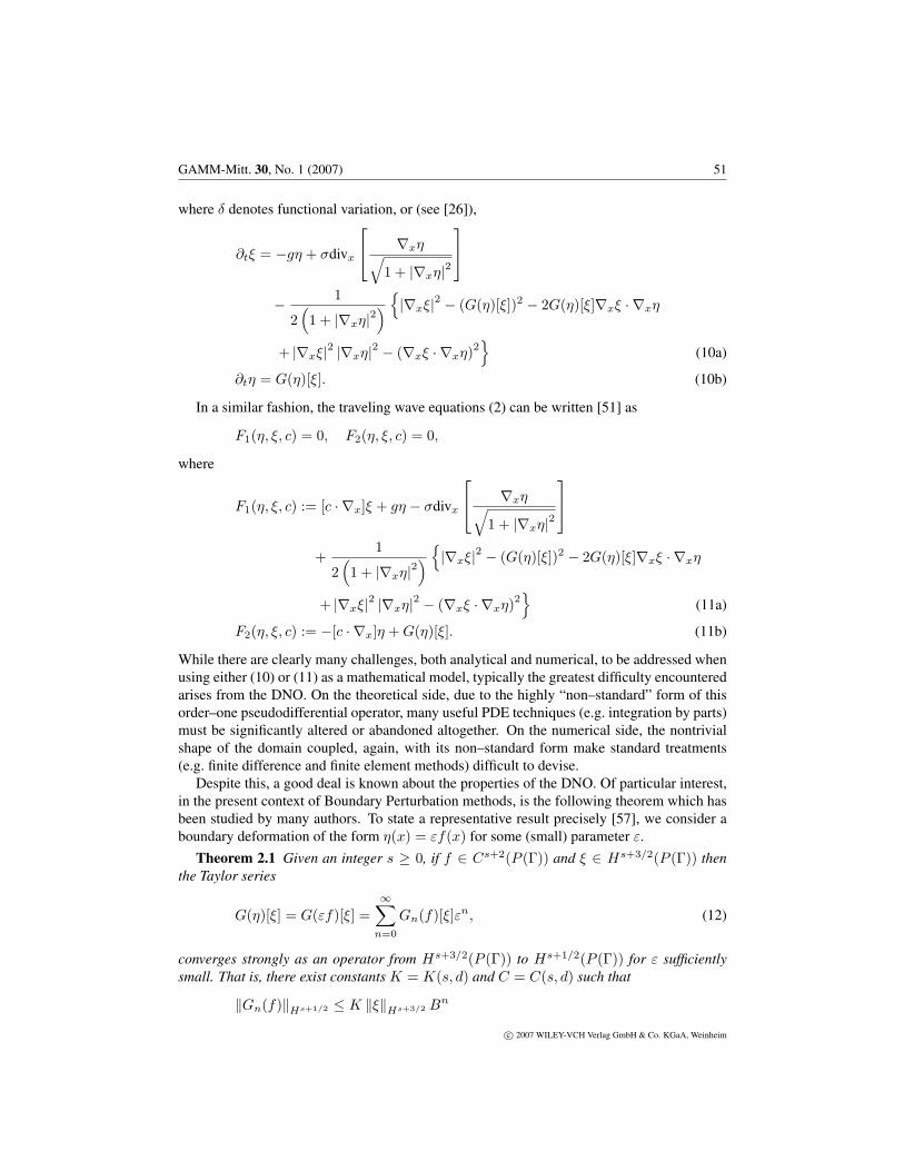
GAMM-Mitt. 30, No. 1 (2007) 51

where δ denotes functional variation, or (see [26]),

∂tξ = −gη + σdivx

⎡⎣ ∇xη√

1 + |∇xη|2

⎤⎦

− 1

2(1 + |∇xη|2

) {|∇xξ|2 − (G(η)[ξ])2 − 2G(η)[ξ]∇xξ · ∇xη

+ |∇xξ|2 |∇xη|2 − (∇xξ · ∇xη)2}

(10a)

∂tη = G(η)[ξ]. (10b)

In a similar fashion, the traveling wave equations (2) can be written [51] as

F1(η, ξ, c) = 0, F2(η, ξ, c) = 0,

where

F1(η, ξ, c) := [c · ∇x]ξ + gη − σdivx

⎡⎣ ∇xη√

1 + |∇xη|2

⎤⎦

+1

2(1 + |∇xη|2

) {|∇xξ|2 − (G(η)[ξ])2 − 2G(η)[ξ]∇xξ · ∇xη

+ |∇xξ|2 |∇xη|2 − (∇xξ · ∇xη)2}

(11a)

F2(η, ξ, c) := −[c · ∇x]η + G(η)[ξ]. (11b)

While there are clearly many challenges, both analytical and numerical, to be addressed whenusing either (10) or (11) as a mathematical model, typically the greatest difficulty encounteredarises from the DNO. On the theoretical side, due to the highly “non–standard” form of thisorder–one pseudodifferential operator, many useful PDE techniques (e.g. integration by parts)must be significantly altered or abandoned altogether. On the numerical side, the nontrivialshape of the domain coupled, again, with its non–standard form make standard treatments(e.g. finite difference and finite element methods) difficult to devise.

Despite this, a good deal is known about the properties of the DNO. Of particular interest,in the present context of Boundary Perturbation methods, is the following theorem which hasbeen studied by many authors. To state a representative result precisely [57], we consider aboundary deformation of the form η(x) = εf(x) for some (small) parameter ε.

Theorem 2.1 Given an integer s ≥ 0, if f ∈ Cs+2(P (Γ)) and ξ ∈ Hs+3/2(P (Γ)) thenthe Taylor series

G(η)[ξ] = G(εf)[ξ] =∞∑

n=0

Gn(f)[ξ]εn, (12)

converges strongly as an operator from Hs+3/2(P (Γ)) to Hs+1/2(P (Γ)) for ε sufficientlysmall. That is, there exist constants K = K(s, d) and C = C(s, d) such that

‖Gn(f)‖Hs+1/2 ≤ K ‖ξ‖Hs+3/2 Bn



for B > C |f |Cs+2 .

This result was first proven by Coifman & Meyer [14], using the theory of Calderon[12],for the case d = 2 when f is merely Lipschitz. This integral equation based approach wasextended to three dimensions (for f ∈ C1) by Craig, Schanz, and Sulem [25], and to arbitrarydimensions by Craig and Nicholls [23, 50]. Theorem 2.1 was proven by Nicholls & Reitich[55, 57] using a quite different method, based upon domain transformation, which inspiredthe numerical algorithm outlined in § 2.6. This method has been subsequently generalized tothe Helmholtz equation by Nicholls & Nigam [53, 54] for applications arising in electromag-netics, and refined by Hu & Nicholls [39] to admit Lipschitz profiles in arbitrary dimensions,thereby extending the original result of Coifman & Meyer to higher dimension.

For numerical simulations the importance of the expansion (12) and Theorem 2.1 goesbeyond the theoretical, and has quite important practical implications as they form the theo-retical foundation for “Boundary Perturbation” (BP) techniques for computing DNO. In § 2.4,§ 2.5, and § 2.6 we outline three algorithms for computing the Gn from (12), and we recallthat these three BP algorithms for the computation of DNO have quite different propertiesin regard to numerical conditioning and computational complexity [56]. In § 5 we demon-strate how these can be combined into a new algorithm which possesses the strengths of bothwhile ameliorating their weaknesses. Clearly, such an advance will have a huge impact onthe numerical simulation of water waves in specific, and boundary value and free boundaryproblems in general.

2.4 Computation of Dirichlet–Neumann Operators: Operator Expansions

In the current exposition of Boundary Perturbation (BP) methods for computing DNO we willrestrict ourselves to the setting of an ocean of infinite depth (h = ∞) and periodic boundaryconditions. Of course formulas for the finite depth case (h < ∞) can also be derived (pleasesee, e.g., [26, 55, 56]), but are somewhat more cumbersome.

The “Operator Expansions” (OE) strategy [82, 49, 26] to approximating DNO deals exclu-sively with the operator, G, and seeks its action on the basis functions eip·x. The OE approachbegins with the observation that

ϕp(x, y) := eip·x+|p|y (13)

satisfies (7a) & (7c). We now insert this “test function” into the definition of the DNO, (8),

G(η)[eip·x+|p|η

]= [|p| − ∇xη · (ip)] eip·x+|p|η.

Recalling that we have set η = εf , and expanding the DNO and exponentials in powers of ε,we find: ( ∞∑

n=0

Gn(f)εn

) [ ∞∑n=0

fn

n!|p|n eip·x

]= [|p| − ε∇xf · (ip)]

[ ∞∑n=0

fn

n!|p|n eip·x

].

At order zero in ε we discover that

G0

[eip·x]

= |p| eip·x,


GAMM-Mitt. 30, No. 1 (2007) 53

and, provided that ξ can be represented by its Fourier series,

ξ(x) =∑p∈Γ′

ξpeip·x, (14)

define the following order–one Fourier multiplier

G0[ξ] = G0

⎡⎣∑

p∈Γ′ξpe

ip·x

⎤⎦ =

∑p∈Γ′

ξpG0

[eip·x]

=∑p∈Γ′

|p| ξpeip·x =: |D| ξ,

where D := (1/i)∇x. Equating at order n in ε we obtain

Gn(f)[eip·x]

=fn

n!|p|n+1

eip·x − fn−1

(n − 1)!∇xf · (ip) |p|n−1

eip·x

−n−1∑l=0

Gl(f)[

fn−l

(n − l)!|p|n−l

eip·x]

.

Using the Fourier multiplier notation |D| and the fact that any sufficiently smooth ξ can berepresented as a sum of complex exponentials we derive

Gn(f)[ξ] =fn

n!|D|n+1

ξ − fn−1

(n − 1)!∇xf · ∇x |D|n−1

ξ

−n−1∑l=0

Gl(f)[

fn−l

(n − l)!|D|n−l

ξ

].

Finally, |D|2 = D · D so that the first two terms can be combined to yield

Gn(f)[ξ] = D ·[fn

n!D |D|n−1

ξ

]−

n−1∑l=0

Gl(f)[

fn−l

(n − l)!|D|n−l

ξ

]. (15)

Now (15) specifies a numerical algorithm once we define how the convolution products arecomputed; this, of course, is done via Fast Fourier Transform (FFT) acceleration. We nowtake up a careful accounting of the computational complexity of this method, and, for this, letus consider the d = 2 dimensional case with Nx Fourier modes and N perturbation orders.Clearly, the bottleneck in the computation of (15) is the term

Xn,l := Gl(f) [Yn,l] ,

Yn,l :=fn−l

(n − l)!|D|n−l

ξ.

Of course, the cost of computing Yn,l (for (n, l) fixed) is O(Nx log(Nx)). However, the naiveapproach to forming the Xn,l is to apply Gl to Yn,l from (15), and involves computing Gm forall 0 ≤ m < l. This scheme will have computational complexity O(N !), however, this enor-mous cost can be greatly reduced by storing the Gl as matrices (which act upon discretized



complex exponentials) and simply performing a matrix–vector product to find Xn,l. The costof computing Gn[eip·x], given all Gl as matrices, is O(nN2

x); this must be completed for Nx

discrete complex exponentials and 0 ≤ n ≤ N orders so the total computational complexityis O(N2N3

x) while the storage is O(NN2x).

However, dramatic computational savings can be realized upon utilization of the self–adjointness property of the DNO. Noting the self–adjointness of D and |D|, we computeG∗

n, which equals Gn,

Gn(f)[ξ] = G∗n(f)[ξ]

= (|D|n−1)∗D∗ ·[fn

n!D∗ξ

]−

n−1∑l=0

(|D|n−l)∗fn−l

(n − l)!G∗

l (f) [ξ]

= |D|n−1D ·

[fn

n!Dξ

]−

n−1∑l=0

|D|n−l fn−l

(n − l)!Gl(f) [ξ] . (16)

Here we notice that the operator Gl always acts upon the same argument, ξ, thus we canstore Gl(f)[ξ], rather than the entire operator Gl, and compute Gn in time proportionalto O(nNx log(Nx)). Consequently the total complexity for all orders 0 ≤ n ≤ N isO(N2Nx log(Nx)), while the storage is merely O(NNx).

2.5 Computation of Dirichlet–Neumann Operators: Field Expansions

In contrast to the Operator Expansions method, which works directly with the operator G, the“Field Expansions” (FE) approach [5, 31] begins with an expansion of the field v, which alsodepends analytically on ε [55, 57], and then produces the Gn from the expansion terms, vn.To start,

v = v(x, y; ε) =∞∑

n=0

vn(x, y)εn,

which, upon insertion into (7), demands that

∆vn = 0 y < 0 (17a)

vn(x, 0) = Hn(x) (17b)∂yvn → 0 y → −∞, (17c)

at every order n where

Hn(x) = δn,0ξ(x) −n−1∑l=0

fn−l

(n − l)!∂n−l

y vl(x, 0),

and δn,k is the Kronecker delta. We recall that solutions vn of (17a) & (17c) can be written as

vn(x, y) =∑p∈Γ′

ap,neip·x+|p|y. (18)


GAMM-Mitt. 30, No. 1 (2007) 55

Given that ξ(x) can be expressed by its Fourier series (14), (17b) delivers a recursion formulafor the ap,n:

ap,n = δn,0ξp −n−1∑l=0

∑q∈Γ′

Cn−l,p−q |q|n−laq,l, (19)

where the Cl,p are defined by

f(x)l

l!=:

∑p∈Γ′

Cl,peip·x.

Simply stated, the FE algorithm is (19) from which velocity potential information can berecovered, in particular the normal derivative at the surface, i.e. the DNO.

To compute the DNO we note that

∞∑n=0

Gn(f)[ξ]εn = G(εf)[ξ] = [∂yv − (ε∇xf)∇xv]y=εf

=∞∑

n=0

∑p∈Γ′

(|p| − (ε∇xf) · (ip))ap,neip·x+|p|εf .

From this we deduce that

Gn(f) =n∑

l=0

fn−l

(n − l)!

∑p∈Γ′

|p|n−l+1ap,le

ip·x

−n−1∑l=0

fn−l−1

(n − l − 1)!∇xf ·

∑p∈Γ′

(ip) |p|n−l−1ap,le

ip·x. (20)

In using (19) & (20) for the numerical simulation of DNO the algorithm is completely deter-mined once we specify that the convolutions are computed by FFT acceleration. Thus, for asimulation in d = 2 dimensions using Nx collocation points and N perturbation orders, thecomputational complexity both for (19) and (20) is O(N2Nx log(Nx)) while the storage isO(NNx).

2.6 Computation of Dirichlet–Neumann Operators: Transformed Field Ex-pansions

While the Operator Expansions (16) and Field Expansions (19) & (20) algorithms each pro-vide a rapid, easily implemented scheme for the simulation of DNO, they do have shortcom-ings. For a wide range of profiles, f , and sizes, ε, both algorithms provide robust, high–orderresults (see, e.g., [26, 5, 6, 7, 8, 9, 10]), however, as the roughness of f and/or the magnitudeof ε is increased subtle cancellations in the OE and FE formalisms become apparent. This hasbeen studied in great detail in the work of Nicholls & Reitich [55, 56, 57, 58, 59, 60, 61] andwe recall some results and consequences of these studies in this section.

We note that neither the OE nor FE algorithms can be used to construct an analyticityproof for the DNO; as we have shown [55], such a strategy is thwarted by the cancellations



mentioned above which are destroyed upon use of standard PDE tools such as the triangleinequality in a Sobolev space. To overcome this numerical ill–conditioning we [55] soughtout a direct, Boundary Perturbation proof for the analyticity of the DNO. We identified sucha method by augmenting the FE approach with a preliminary transformation, producing the“Transformed Field Expansion” (TFE) algorithm. Before discussing the details, we restatethe problem (7) on a truncated domain which not only allows for a unified statement of resultsfor finite and infinite depth, but also delivers a much faster numerical algorithm.

Consider a hyperplane y = −a strictly below the surface of the ocean (a > |η|L∞ ), yetabove the bottom of the ocean (a < h). Our goal is to equivalently state (7) on the truncateddomain Sa,η. With this in mind we consider the augmented DNO problem

∆v = 0 − a < y < η(x) (21a)

v(x, η(x)) = ξ(x) (21b)

∂yv(x,−a) = ∂yw(x,−a) (21c)

v(x,−a) = w(x,−a) (21d)∆w = 0 − h < y < −a (21e)

∂yw(x,−h) = 0, (21f)

where, clearly, the solutions (v, w) of (21) “match” those of (7) in that the v are equal on Sa,η,while v = w on −h < y < −a. We now gather (21d)–(21f) as

∆w = 0 − h < y < −a

w(x,−a) = ζ(x)

∂yw(x,−h) = 0,

where ζ(x) stands for v(x,−a), and notice that these equations have the exact solution

w(x, y) =∑p∈Γ′

ζpcosh(|p| (y + h))cosh(|p| (h − a))

eip·x.

Equation (21c) requires the normal derivative ∂yw thus we construct a second DNO:

T [ζ] : = ∂yw(x,−a)

=∑p∈Γ′

|p| tanh(|p| (h − a))ζpeip·x

= |D| tanh((h − a) |D|)ζ,

and (21a)–(21c) can now be stated entirely in terms of v as

∆v = 0 − a < y < η(x) (22a)

v(x, η(x)) = ξ(x) (22b)

∂yv(x,−a) − T [v(x,−a)] = 0. (22c)


GAMM-Mitt. 30, No. 1 (2007) 57

Equation (22) now provides the restatement of (7) on the truncated domain Sa,η via a “trans-parent boundary condition” at y = −a [60, 61].

We now discuss the TFE method for computing the Gn in the Taylor expansion of theDNO. Consider the (non–conformal) change of variables,

x′ = x, y′ = a

(y − η

a + η

), (23)

which maps Sa,η to Sa,0. We find that the transformed potential

u(x′, y′) = v(x′, ((a + η(x′))/a)y′ + η(x′)),

must satisfy

∆′u = F (x′, y′; u) − a < y′ < 0

u(x′, 0) = ξ(x′)

∂y′u(x′,−a) − T [u(x′,−a)] = Q(x′; u),

where the precise forms of F and Q are given in [55, 56, 57]. In these papers it was shownthat the transformed potential, u, is also analytic in ε so that we may make, upon droppingprimes, the expansion

u(x, y; ε) =∞∑

n=0

un(x, y)εn.

It is not hard to show that the un must satisfy

∆un = Fn(x, y) − a < y < 0 (24a)

un(x, 0) = δn,0ξ(x) (24b)

∂yun(x,−a) − T [un(x,−a)] = Qn(x), (24c)

where the Fn and Qn are again given in [55, 56, 57]. From this the n–th term in the expansionof the DNO can be found from

Gn(f)[ξ] = ∂yun(x, 0) − f

hGn−1(f)[ξ] −∇xf · ∇xun−1(x, 0)

− f

h∇xf · ∇xun−2(x, 0) + |∇xf |2 ∂yun−2(x, 0).

Complete details with a full discussion of implementation issues and numerical results canbe found in [56]. From this we recall that, in contrast to the OE and FE procedures, anddue to the inhomogeneous nature of the Poisson equation (24a), we are unable to solve (24)without a discretization of the y–variable. We can partially ameliorate this difficulty with theuse of a fast, Chebyshev spectral method [34, 13] at a cost O(Ny log(Ny)) per order n andwavenumber k, where Ny is the number of Chebyshev polynomials utilized. Also, with thedomain truncated at y = −a we can choose a quite small in the hope that Ny need not bechosen very large. However, the total execution time is O(NNx log(Nx)Ny log(Ny)) and thetotal storage is O(NNxNy).



Despite this disadvantaged operation count, as compared with other BP methods, the in-creased accuracy and stability of the TFE method renders it the most compelling option inmany applications. We will return to these points in § 5 as they provide the impetus for one“future direction” we foresee in BP methods for water waves and other boundary value andfree boundary problems: The combination of the FE and TFE algorithms to produce a rapidand stable high–order method.

3 Boundary Perturbation Methods for the Initial Value Problem

Several authors have investigated Boundary Perturbation techniques for the approximation ofthe water wave initial value problem (1). These generally fall into one of the two categories:Those that deal directly with the full Euler equations (1), and those that approximate thesurface formulation (10) of Zakharov [86] and Craig & Sulem [26].

Examples of Boundary Perturbation approaches to (1) are the work of Fenton & Rienecker[33] who studied solitary wave interactions of the full Euler equations, and Dommermuth &Yue [31]. In these methods one assumes that the quantities η and ϕ depend analytically on thesmall parameter ε (representing the height/slope of the wave) and insert the Taylor expansions

η(x, t; ε) =∞∑

n=1

ηn(x, t)εn, ϕ(x, y, t; ε) =∞∑

n=1

ϕn(x, y, t)εn,

directly into (1). These are then equated at orders of ε, and a modal expansion of the ηj andϕj results in a set of time–dependent coefficients that must be evolved. For derivatives ofηj and tangential derivatives of ϕj this is straightforward, however, for normal derivatives ofthe velocity potential the modes are coupled in a complicated way. Of course this is to beexpected as this operation is simply the DNO discussed in § 2.3.

Zakharov’s Hamiltonian formulation of the water wave problem [86] was pursued by Wat-son & West [81], and West, Brueckner, Janda, Milder, and Milton [82] to produce a numericalalgorithm based upon Boundary Perturbation of the Hamiltonian (9). While the languageof the DNO was not used, the operators |D| and convolutions (written as commutators) areclearly evident. Craig & Sulem [26], Schanz [74], and Guyenne & Nicholls [36] all use (10)as their starting point and approximate the DNO, rather than the Hamiltonian, by its truncation

GN (η)[ξ] :=N∑

n=0

Gn(η)[ξ].

Craig & Sulem [26] considered the two–dimensional case in the absence of capillarity, whileSchanz [74] generalized to three dimensions in the presence of surface tension. Guyenne &Nicholls [36] studied two–dimensional gravity waves over plane slopes (bathymetry) whichrequired a generalization of the DNO to include bottom topography. Please see Smith [78];Craig, Guyenne, Nicholls, and Sulem [22]; and Nicholls and Taber [63] for more details onthis extension. Recently, Craig, Guyenne, Hammack, Henderson, and Sulem [20] used thisapproach to revisit the problem of solitary wave interactions and compared the results withthose of wave–tank experiments. Finally, we point out the work of de la Llave & Panayotaros[29] on the simulation of gravity waves on the sphere. Of course, the water wave equationsdo not provide a useful model for the ocean on the surface of the earth, however, it is aninteresting and non–trivial extension of this approach to spherical geometries.


GAMM-Mitt. 30, No. 1 (2007) 59

4 Boundary Perturbation Methods for Traveling Waves

As we mentioned in the Introduction, with the availability of convenient and spectrally accu-rate integral equations methods, little effort has been expended upon the investigation of trav-eling two–dimensional water waves using Boundary Perturbation techniques (however, see[24] for some two–dimensional BP results). For this reason we will focus, for the rest of thissection, upon the problem of simulating genuinely three–dimensional traveling waveforms. Inthis setting Boundary Perturbation methods have been applied to not only the original Eulerequations (2), but also the surface formulation (11) and the transformed Euler equations (26).

In the case of the original Euler equations (2) the work of Roberts [70], Roberts & Pere-grine [71], and Marchant & Roberts [47] is definitive in the absence of surface tension (itappears, however, that the subtleties of the existence theory for pure gravity waves in three di-mensions was not properly appreciated by these authors, see § 2.2). We also note the closelyrelated work of Roberts & Schwartz [72] which also considered the computation of three–dimensional traveling waves, but did not utilize a BP approach. All of these BP methodspostulate Taylor expansions of the form

η(x; ε) =∞∑

n=1

ηn(x)εn, ϕ(x, y; ε) =∞∑

n=1

ϕn(x, y)εn, c(ε) =∞∑

n=0

cnεn (25)

and insert these directly into (2). Equating at orders of ε one recovers, at order one, the lin-ear solutions (6) provided that c0 satisfies (5) for two wavenumbers k1 and k2. At higherorders, the perturbative procedure delivers a linear inhomogeneous PDE to be solved for theunknowns (ηn, ϕn, cn−1). The linear operator in this PDE is (3) which is, of course, singu-lar precisely by the choice of c0; however, the parameter cn−1 can be chosen to verify theassociated solvability condition, and several parameterizations of the bifurcation curve areavailable which select a unique solution. We refer the interested reader to [60] for a completespecification of this method using the particular notations used in the present paper. Onceagain, the real issue with this method is the evaluation of normal derivatives of the velocitypotential at the free surface. Roberts et al chose to implement an algorithm similar to that ofthe FE method presented in § 2.5, however, the details are complicated by the fact that onemust evaluate these quantities not simply at a profile which depends linearly on ε (η = εf )but rather in a nonlinear, though analytic, fashion, c.f. (25). Consequently, this algorithm hascomputational complexity O(N3N2

1 N22 ) for a simulation involving N perturbation orders and

N1 × N2 spatial collocation points. In addition, this method, much like the FE algorithm, isseverely ill–conditioned for N large (please see [60, 61] for demonstrations).

Of course the conditioning properties of methods based on (11) depend strongly upon theimplementation of the DNO: High–order numerics based upon OE and FE implementationswill be rather unstable, while those using the TFE method will enjoy much greater stability,at perhaps a slightly higher computational cost (see § 2.4, § 2.5, and § 2.6). The computationsof Nicholls [50, 51], and Craig & Nicholls [24] were based on an OE implementation of theDNO, but were performed at a relatively low perturbation order, N = 5. These simulationsutilized Boundary Perturbations solely in the computation of the DNO and otherwise usednumerical continuation [42, 2] to find solutions of (11) along the branch using a predictor–corrector algorithm.

In quite recent work, Nicholls & Reitich [61] numerically approximated the transformed re-cursions for traveling water waves derived in [60] using a Fourier/Chebyshev spectral method.



The derivation of these equations is quite similar to that presented in § 2.6 and, in fact, thechange of variables (23) is identical. This transformation is applied to (2) (modified to in-clude a “transparent boundary condition,” c.f. (22)) and results, for the unknowns η, c, andthe transformed potential

u(x′, y′) = ϕ(x′, (a + η(x′))y′/a + η(x′)),

in the following system of equations (upon dropping primes):

∆u = F (x, y; u) − a < y < 0 (26a)

∂yu(x,−a) − Tu(x,−a) = J(x; u) (26b)

[c0 · ∇x] u + [g − σ∆x] η = Q(x; u) at y = 0 (26c)

− [c0 · ∇x] η + ∂yu = R(x; u) at y = 0, (26d)

where the forms of F , J , Q, and R are given in [61].Following the Field Expansions philosophy we posit the expansions

η(x; ε) =∞∑

n=1

ηn(x)εn, ϕ(x, y; ε) =∞∑

n=1

ϕn(x, y)εn, c(ε) =∞∑

n=0

cnεn.

These (ηn, un, cn−1) are governed by

∆un = Fn(x, y) − a < y < 0 (27a)

∂yun(x,−a) − Tun(x,−a) = Jn(x) (27b)

[c0 · ∇x] un + [g − σ∆x] ηn = Qn(x) − [cn−1 · ∇x] u1 at y = 0 (27c)

− [c0 · ∇x] ηn + ∂yun = Rn(x) + [cn−1 · ∇x] η1 at y = 0, (27d)

where the Fn, Jn, Qn, and Rn can be found in [61]. Here η1 and u1 are linear solutions (c.f.(6)) provided c0 satisfies (5) and, again, the linear operator (3) appears on the left–hand sideof (27). As with the approach of Roberts et al [70, 47], the velocity cn−1 is used to satisfythe solvability condition required by the singular nature of the system (27), while severalparameterizations of the bifurcation curve can be given which produce a unique solution atevery order; please see [61] for details.

On the theoretical side, Reeder & Shinbrot [68] proved the existence of solution branchesto (26) and parametric (i.e. with respect to ε) analyticity using the perturbative approachoutlined above. Their strategy required that not only σ > 0 but also the absence of resonance(see § 2.2). Craig & Nicholls [23] extended these results with an application of the Lyapunov–Schmidt theory to (11) and noted that solutions come in surfaces rather than simply branches.Their analysis still required σ > 0 but permitted “finite” resonance (provided that p < ∞,see § 2.2). Nicholls & Reitich [60] extended the method of Reeder & Shinbrot by not onlyverifying, quite directly, that solutions do come in surfaces, by making expansions of the form

η(x; ε1, ε2) =∑

n1+n2≥1

ηn1,n2(x)εn11 εn2

2 ,

but also by showing that the velocity potential and traveling wave surface are jointly analyticwith respect to both parameters (ε1, ε2) and spatial variables (x, y).


GAMM-Mitt. 30, No. 1 (2007) 61

On the computational side, Nicholls & Reitich [61] showed that the TFE recursions forwater waves (27) could be converted into a rapid, high–order, stable numerical method forcomputing traveling water waves. Not only does this method enjoy the stability properties ofthe TFE method for DNO (as compared to the OE and FE implementations), but also, andin contrast to the situation for computing DNO, it has a greatly reduced operation count incomparison to the Roberts algorithm. In fact, we showed that the computational complexityis

O(NN1N2 log(Ny)Ny + N2N1N2Ny)

to be compared with O(N3N21 N2

2 ) for Roberts [70] and Marchant & Roberts [47]. With thisefficiency and high–order stability we are now able to produce extremely accurate simulationsof highly nonlinear waveforms as we now demonstrate.

For this we revisit the calculations of Nicholls & Reitich [61] and specialize to the geometryof the “short–crested waves” (SCW) [70]. A short–crested wave is a traveling waveform that isnot only periodic in the direction of propagation, but also periodic in the orthogonal horizontaldirection. The period in the propagation direction is set to L/ sin(θ) while the period in theorthogonal direction is L/ cos(θ). If we choose the x1–axis as the direction of propagationand non–dimensionalize by setting L = 2π, the solutions will be periodic with respect to thelattice

Γθ = {γ = j1a + j2b | a = (2π)/ sin(θ), b = (2π)/ cos(θ); j1, j2 ∈ Z}, (28)

i.e. η(x + γ) = η(x) for all γ ∈ Γθ. We also consider the case of water of infinite depth(h = ∞), and in all calculations the numerical parameters were set to N1 = N2 = 64(Fourier modes in the horizontal directions), Ny = 48 (Chebyshev coefficients in the verticaldirection), and N = 31 (perturbation orders).

For each of three values of θ = 45o, 60o, 75o we selected two values of the parameterε which were meant to prescribe “moderately nonlinear,” and “highly nonlinear” profiles.We summarize these choices and our results in Table 1. Furthermore, in Figures 1–12 wereproduce plots of these solutions from [61]. From this it is easy to see how the waves becomemore nonlinear (with sharper, narrower crests and wider, shallower troughs) as ε is increased.Also, notice how the “shape” of the wave deforms from diamond–like to rectangular as θis increased, in nice agreement with the experimental results of Hammack, Henderson, andSegur [37, 38].

5 Future Directions: Rapid and Stable High–Order Methods

As we have seen, Boundary Perturbation methods provide a fast, stable, and highly accuratemethod for the simulation of water waves. However, the stabilized methods we advocate herecan be slightly disadvantaged in terms of computational complexity in comparison with otherschemes (e.g. for the computation of DNO). One direction of future research is to address thisconcern with the development of methods with the speed of the FE recursions which retainthe stability and accuracy properties of the TFE procedure. We now present a novel algorithmbased upon the FE philosophy, but inspired by the success of the TFE scheme, to achieveprecisely these requirements. For this discussion of “future directions” we restrict ourselvesto the computation of DNO, however, it should be clear how to extend these ideas to moregeneral situations.



Table 1 Summary of traveling wave calculations.

Figure θ ε |η(x; ε)|L∞ Plot Type

Figure 1 45o 0.21 0.224997 Surface


Figure 3 45o 0.21 0.224997 Contour










Fig. 1 Surface plot of ocean profile withθ = 45o and ε = 0.21.


5.1 Stabilized Field Expansions

The success of the TFE method for computing DNO in a stable, high–order fashion is thatthe change of variables enforces that all derivatives be taken inside the problem domain. Bycontrast, the FE recursions require the differentiation of the field at y = 0 which is sometimesacross the boundary of the problem domain. With this in mind we consider a number b >|η|L∞ and the family of surfaces which are strictly interior to the domain,

σδ(x; b) := (1 − δ)(−b) + δη(x) = −b + δ(η(x) + b);


GAMM-Mitt. 30, No. 1 (2007) 63

0 5 10 15 200

2

4

6

8

10

12

14

16

Fig. 3 Contour plot of ocean profile withθ = 45o and ε = 0.21.

0 5 10 15 200

2

4

6

8

10

12

14

16




−5 0 5 10 15 200

5

10

15

20

25


−5 0 5 10 15 200

5

10

15

20

25


note that σ0 = −b and σ1 = g(x), i.e. σδ provides a homotopy from the hyperplane y = −bto the ocean surface y = η. We will now consider δ as our expansion parameter and expand





−20 −10 0 10 20 300

5

10

15

20

25

30

35

40

45


−20 −10 0 10 20 300

5

10

15

20

25

30

35

40

45


the field

v = v(x, y; δ) =∞∑

n=0

vn(x, y)δn,

where, to find quantities at the ocean surface, we evaluate at δ = 1. To find the vn we lookto (7) and note that v satisfies both Laplace’s equation for y < σδ , and equation (7c). The


GAMM-Mitt. 30, No. 1 (2007) 65

Dirichlet condition (7b) implies

ξ(x) = v(x, σδ; δ)|δ=1

=

[ ∞∑n=0

vn(x, σδ)δn

]δ=1

=

[ ∞∑n=0

vn(x,−b + δ(η + b))δn

]δ=1

=

[ ∞∑n=0

( ∞∑m=0

(η + b)m

m!∂m

y vn(x,−b)δm

)δn

]δ=1

=

[ ∞∑n=0

δnn∑

l=0

(η + b)n−l

(n − l)!∂n−l

y vl(x,−b)

]δ=1

.

Therefore we can write the analogue of (17b):

vn(x,−b) = δn,0ξ(x) −n−1∑l=0

(η + b)n−l

(n − l)!∂n−l

y vl(x,−b).

Since vn can be expressed as

vn(x, y) =∑p∈Γ′

dp,neip·x+|p|y,

c.f. (18), it is easy to show that

dp,n = e|p|b

⎧⎨⎩δn,0ξp −

n−1∑l=0

∑q∈Γ′

Kn−l,p−qe−|q|b |q|n−l

dq,l

⎫⎬⎭ , (29)

where the Kl,p are defined by

(η + b)l

l!=:

∑p∈Γ′

Kl,peip·x.

Defining the pseudodifferential operator SD as

SD[ψ] :=∑p∈Γ′

Spψpeip·x =

∑p∈Γ′

e−|p|bψpeip·x,

and identifying its inverse

S−1D [ψ] =

∑p∈Γ′

S−1p ψpe

ip·x =∑p∈Γ′

e|p|bψpeip·x,

we rewrite (29) as

dp,n = S−1p

⎧⎨⎩δn,0ξp −

n−1∑l=0

∑q∈Γ′

Kn−l,p−qSq |q|n−ldq,l

⎫⎬⎭ . (30)



With this notation we point out some of the advantages and shortcomings of this “modified”Field Expansions method,(30). Clearly, the operator SD is “infinitely smoothing” (mapping,for instance, L2 functions to the class of real analytic functions) and we can hope that thisoperator will “smooth away” errors magnified by the order (n− l) pseudodifferential operator|D|n−l. However, the operator S−1

D must also be applied and this will, at all scales, exponen-tially amplify truncation errors. To ameliorate this effect we introduce the modified operatorBF

D:

BFD[ψ] :=

∑p∈Γ′

BFp ψpe

ip·x, BFp :=

{e|p|b |p| ≤ F

0 |p| > F,

and now define the Stabilized Field Expansions (SFE) method as

dp,n = BFp

⎧⎨⎩δn,0ξp −

n−1∑l=0

∑q∈Γ′

Kn−l,p−qSq |q|n−ldq,l

⎫⎬⎭ . (31)

In § 5.3 we will present some preliminary numerical results showing how this algorithm,combined with the ideas of § 5.2 on Dirichlet–Interior Derivative Operators, can give greatlyenhanced numerical results, as compared to an FE implementation, with the same computa-tional complexity.

5.2 Dirichlet–Interior Derivative Operators

Following the philosophy of [59], to compute the DNO we consider a family of “Dirichlet–Interior Derivative Operators” (DIDO) which evaluate the “normal derivative,” ∇v ·Nη, at theinterior surface σδ introduced above. As discussed in [59], this operation should be largelyfree from the severe cancellations present in formulas (19) & (20) since no derivatives of thefield are taken across the boundary y = η(x). Of course, to compute the actual DNO we mustevaluate at the surface y = η(x), i.e. at δ = 1.

We define our family of DIDO as

G(δ)[ξ] := [∇v · Nη]y=σδ= [∂yv −∇xη · ∇xv]y=σδ

,

for every 0 ≤ δ ≤ 1. To compute these DIDO we expand

G(δ)[ξ] =∞∑

n=0

Gn[ξ]δn,

and, using the SFE computations above, equate

∞∑n=0

Gn[ξ]δn = [∂yv −∇xη · ∇xv]y=σδ

=∞∑

n=0

∑p∈Γ′

(|p| − ∇xη · (ip))dp,neip·x−|p|b+|p|δ(η+b)δn.


GAMM-Mitt. 30, No. 1 (2007) 67

From this we deduce that

Gn =∑p∈Γ′

n∑l=0

Kn−l(|p| − ∇xη · (ip))e−b|p| |p|n−ldp,l, (32)

where

Kl :=(η(x) + b)l

l!.

Notice that in this computation there is never a need to apply the operator S−1D and, thus, no

need to use the approximating operator BFD.

So, our new computational strategy of Stabilized Field Expansions and Dirichlet–InteriorDerivative Operators (SFE/DIDO) for computing Dirichlet–Neumann operators amounts tousing (31) to compute the coefficients dp,n followed by the utilization of (32) to recover thenormal derivative. The computational complexity of these two steps is identical to that of theoriginal FE method (19) & (20), namely O(N2Nx), while the storage is merely O(NNx). Ofcourse there are two parameters to choose, b and F , which will greatly affect the performanceof this new method. For instance, if b is chosen too close to zero then the method will behavemuch like the FE algorithm and we have achieved nothing new. If b is chosen too large then the“base” for our homotopy will be too far from the surface and we cannot expect good results. Itis the subject of current research by Nicholls & Reitich [62], in the setting of electromagneticand acoustic scattering, to provide guiding principles for the choice of these parameters.

5.3 Numerical Results

In this section we will show some preliminary results to illustrate the effectiveness of our newSFE/DIDO algorithm (§ 5.1 and § 5.2) for computing DNO. For simplicity we will restrictourselves to the two dimensional setting (periodic on the interval [0, 2π]) for an ocean ofinfinite depth (h = ∞). For this we will take advantage of a family of exact solutions of theelliptic problem (7) which, for an arbitrary profile η = εf , can be used to specify Dirichletdata and produces exact Neumann data. This family of solutions is

vp(x, y) := eip·x+|p|y,

for p ∈ Γ′, c.f. (13), which, given Dirichlet data,

ξp(x) := vp(x, η(x)) = eip·x+|p|η(x),

produces Neumann data

νp(x) := (∂y −∇xη · ∇x)vp(x, η(x)) = (|p| − ∇xη · (ip))eip·x+|p|η(x). (33)

For all results presented in this section we have set p = 3.We now consider numerical implementations of (19) & (20), which we term the FE method,

and (31) & (32), which we denote the SFE/DIDO procedure. For each we will retain Nx

Fourier modes and N Taylor coefficients. For each mode k ∈ Γ′ in our computation, anyTaylor polynomials, e.g.

τk(ε) :=N∑

n=0

dk,nεn,



are summed either directly (Taylor summation) or using Pade approximation (Pade summa-tion) [3, 6, 7, 56].

In these experiments we will consider two interfaces, a “smooth” profile fs (sinusoidal),and a “rough” profile fr which is C4 but not C5 [58, 59]:

fs(x) = cos(x), (34a)

fr(x) = (2 × 10−4)x4(2π − x)4 − c0, , (34b)

where c0 is chosen so that fr has zero mean. The second of these profiles has an infiniteFourier series representation

fr(x) =∞∑

k=1

96(2k2π2 − 1)125k8

cos(kx),

and, in order to minimize the effects of aliasing, we approximate it by its truncated Fourierseries:

fr,P (x) :=P∑

k=1

96(2k2π2 − 1)125k8

cos(kx). (35)

For the smooth profile fs, in Figures 13–14 we display the relative error, measured inL∞, in computing the normal derivative of the field at the boundary, i.e. the DNO, versusperturbation order N . In these simulations we chose ε = 0.7, while the numerical parameterswere Nx = 256, N = 60, b = 0.0001, 0.01, 1, and F = 16 (Figure 13) or F = 4 (Figure 14).

First, we point out the remarkable stabilizing properties which the SFE/DIDO algorithm

0 10 20 30 40 50 6010

−5

100

105

1010

1015

1020

1025

1030

1035

1040

N

L∞ E

rror

Error (Taylor)

FESFE (b=0.01)SFE (b=0.0001)SFE (b=1)

0 10 20 30 40 50 6010

−8

10−7

10−6

10−5

10−4

10−3

10−2

10−1

100

N

L∞ E

rror

Error (Pade)

FESFE (b=0.01)SFE (b=0.0001)SFE (b=1)

Fig. 13 Relative L∞ error in FE and SFE/DIDO computations of normal derivative at the boundaryfor the smooth profile fs, (34a). Numerical parameters are Nx = 256, N = 60, b = 0.0001, 0.01, 1,F = 16. For the calculation depicted on the left Taylor summation is utilized, while for that on the rightPade summation is used.

possesses: The FE algorithm begins to diverge at N = 9 while the enhanced summation ofPade approximation can only ever deliver accuracy of 10−4. However, our new SFE/DIDOprocedure produces solutions which are increasingly more accurate throughout all orders,though they can be disadvantaged when b is chosen as large as one. Interestingly, the reduction


GAMM-Mitt. 30, No. 1 (2007) 69

0 10 20 30 40 50 6010

−20

10−10

100

1010

1020

1030

1040

N

L∞ E

rror

Error (Taylor)

0 10 20 30 40 50 6010

−15

10−10

10−5

100

N

L∞ E

rror

Error (Pade)

FESFE (b=0.01)SFE (b=0.0001)SFE (b=1)

FESFE (b=0.01)SFE (b=0.0001)SFE (b=1)

Fig. 14 Relative L∞ error in FE and SFE/DIDO computations of normal derivative at the boundaryfor the smooth profile fs, (34a). Numerical parameters are Nx = 256, N = 60, b = 0.0001, 0.01, 1,F = 4. For the calculation depicted on the left Taylor summation is utilized, while for that on the rightPade summation is used.

in the “operator filter” F has the effect of producing slightly worse results for N small, whileproducing results which are drastically better for N large; for instance, SFE/DIDO reachesonly 10−8 accuracy when F = 16, while it achieves full double precision accuracy whenF = 4 (provided, in these experiments, that b < 1).

Finally, for the rough profile fPr , we display in Figures 15–16 the relative error, measured in

L∞, in computing the DNO versus perturbation order N . In this simulation we again chooseε = 0.7, while the numerical parameters were Nx = 256, N = 60, b = 0.0001, 0.01, 1,P = 40, and F = 16 (Figure 15) or F = 4 (Figure 16). Again, we point out the stable

0 10 20 30 40 50 6010

−5

100

105

1010

1015

1020

1025

1030

1035

1040

N

L∞ E

rror

Error (Taylor)

0 10 20 30 40 50 6010

−7

10−6

10−5

10−4

10−3

10−2

10−1

100

N

L∞ E

rror

Error (Pade)

FESFE (b=0.01)SFE (b=0.0001)SFE (b=1)

FESFE (b=0.01)SFE (b=0.0001)SFE (b=1)

Fig. 15 Relative L∞ error in FE and SFE/DIDO computations of normal derivative at the boundaryfor the rough profile f40

r , (35). Numerical parameters are Nx = 256, N = 60, b = 0.0001, 0.01, 1,F = 16. For the calculation depicted on the left Taylor summation is utilized, while for that on the rightPade summation is used.

nature of the SFE/DIDO method, which produces consistently improved answers throughoutall perturbation orders. Again, this effect is largely independent of the parameter b, thoughb = 1 is clearly disadvantaged in this case. Again, the role of F is significant and it is clear



0 10 20 30 40 50 6010

−20

10−10

100

1010

1020

1030

1040

N

L∞ E

rror

Error (Taylor)

0 10 20 30 40 50 6010

−15

10−10

10−5

100

N

L∞ E

rror

Error (Pade)

FESFE (b=0.01)SFE (b=0.0001)SFE (b=1)

FESFE (b=0.01)SFE (b=0.0001)SFE (b=1)

Fig. 16 Relative L∞ error in FE and SFE/DIDO computations of normal derivative at the boundaryfor the rough profile f40

r , (35). Numerical parameters are Nx = 256, N = 60, b = 0.0001, 0.01, 1,F = 4. For the calculation depicted on the left Taylor summation is utilized, while for that on the rightPade summation is used.

that future research [62] is necessary to not only provide guidance on the choice of b and F ,but also give an explanation for the behavior of this new algorithm.

Acknowledgements The author gratefully acknowledges support from the NSF through grant No. DMS–0537511.

References

[1] Mark J. Ablowitz and Harvey Segur. Solitons and the inverse scattering transform, volume 4 ofSIAM Studies in Applied Mathematics. Society for Industrial and Applied Mathematics (SIAM),Philadelphia, Pa., 1981.

[2] Eugene L. Allgower and Kurt Georg. Numerical continuation methods. Springer-Verlag, Berlin,1990.

[3] George A. Baker, Jr. and Peter Graves-Morris. Pade approximants. Cambridge University Press,Cambridge, second edition, 1996.

[4] J. Thomas Beale. A convergent boundary integral method for three-dimensional water waves.Math. Comp., 70(235):977–1029, 2001.

[5] Oscar P. Bruno and Fernando Reitich. Numerical solution of diffraction problems: A method ofvariation of boundaries. J. Opt. Soc. Am. A, 10(6):1168–1175, 1993.

[6] Oscar P. Bruno and Fernando Reitich. Numerical solution of diffraction problems: A method ofvariation of boundaries. II. Finitely conducting gratings, Pade approximants, and singularities. J.Opt. Soc. Am. A, 10(11):2307–2316, 1993.

[7] Oscar P. Bruno and Fernando Reitich. Numerical solution of diffraction problems: A methodof variation of boundaries. III. Doubly periodic gratings. J. Opt. Soc. Am. A, 10(12):2551–2562,1993.

[8] Oscar P. Bruno and Fernando Reitich. Calculation of electromagnetic scattering via boundaryvariations and analytic continuation. Appl. Comput. Electromagn. Soc. J., 11(1):17–31, 1996.

[9] Oscar P. Bruno and Fernando Reitich. Boundary–variation solutions for bounded–obstacle scatter-ing problems in three dimensions. J. Acoust. Soc. Am., 104(5):2579–2583, 1998.


GAMM-Mitt. 30, No. 1 (2007) 71

[10] Oscar P. Bruno and Fernando Reitich. High-order boundary perturbation methods. In Mathe-matical Modeling in Optical Science, volume 22, pages 71–109. SIAM, Philadelphia, PA, 2001.Frontiers in Applied Mathematics Series.

[11] P. J. Bryant. Doubly periodic progressive permanent waves in deep water. J. Fluid Mech., 161:27–42, 1985.

[12] A. P. Calderon. Cauchy integrals on Lipschitz curves and related operators. Proc. Nat. Acad. Sci.USA, 75:1324–1327, 1977.

[13] Claudio Canuto, M. Yousuff Hussaini, Alfio Quarteroni, and Thomas A. Zang. Spectral methodsin fluid dynamics. Springer-Verlag, New York, 1988.

[14] R. Coifman and Y. Meyer. Nonlinear harmonic analysis and analytic dependence. In Pseudod-ifferential operators and applications (Notre Dame, Ind., 1984), pages 71–78. Amer. Math. Soc.,1985.

[15] W. Craig, C. Sulem, and P.-L. Sulem. Nonlinear modulation of gravity waves: a rigorous approach.Nonlinearity, 5(2):497–522, 1992.

[16] Walter Craig. An existence theory for water waves and the Boussinesq and Korteweg-de Vriesscaling limits. Comm. Partial Differential Equations, 10(8):787–1003, 1985.

[17] Walter Craig. Birkhoff normal forms for water waves. In Mathematical problems in the theoryof water waves (Luminy, 1995), volume 200 of Contemp. Math., pages 57–74. Amer. Math. Soc.,Providence, RI, 1996.

[18] Walter Craig and Mark D. Groves. Hamiltonian long-wave approximations to the water-waveproblem. Wave Motion, 19(4):367–389, 1994.

[19] Walter Craig and Mark D. Groves. Normal forms for wave motion in fluid interfaces. Wave Motion,31(1):21–41, 2000.

[20] Walter Craig, Philippe Guyenne, Joe Hammack, Diane Henderson, and Catherine Sulem. Solitarywave interactions. Phys. Fluids, 18:057106, 2006.

[21] Walter Craig, Philippe Guyenne, and Henrik Kalisch. Hamiltonian long-wave expansions for freesurfaces and interfaces. Comm. Pure Appl. Math., 58(12):1587–1641, 2005.

[22] Walter Craig, Philippe Guyenne, David P. Nicholls, and Catherine Sulem. Hamiltonian long waveexpansions for water waves over a rough bottom. Proc. Roy. Soc. Lond., A, 461(2055):839–873,2005.

[23] Walter Craig and David P. Nicholls. Traveling two and three dimensional capillary gravity waterwaves. SIAM J. Math. Anal., 32(2):323–359, 2000.

[24] Walter Craig and David P. Nicholls. Traveling gravity water waves in two and three dimensions.Eur. J. Mech. B Fluids, 21(6):615–641, 2002.

[25] Walter Craig, Ulrich Schanz, and Catherine Sulem. The modulation regime of three-dimensionalwater waves and the Davey-Stewartson system. Ann. Inst. Henri Poincare, 14:615–667, 1997.

[26] Walter Craig and Catherine Sulem. Numerical simulation of gravity waves. Journal of Computa-tional Physics, 108:73–83, 1993.

[27] Walter Craig and Patrick A. Worfolk. An integrable normal form for water waves in infinite depth.Phys. D, 84(3-4):513–531, 1995.

[28] Michael G. Crandall and Paul H. Rabinowitz. Bifurcation from simple eigenvalues. J. FunctionalAnalysis, 8:321–340, 1971.

[29] R. de la Llave and P. Panayotaros. Gravity waves on the surface of the sphere. J. Nonlinear Sci.,6(2):147–167, 1996.

[30] Frederic Dias and Christian Kharif. Nonlinear gravity and capillary-gravity waves. In Annualreview of fluid mechanics, Vol. 31, pages 301–346. Annual Reviews, Palo Alto, CA, 1999.

[31] Douglas G. Dommermuth and Dick K. P. Yue. A high-order spectral method for the study ofnonlinear gravity waves. Journal of Fluid Mechanics, 184:267–288, 1987.

[32] Lawrence C. Evans. Partial differential equations. American Mathematical Society, Providence,RI, 1998.

[33] J. D. Fenton and M. M. Rienecker. A Fourier method for solving nonlinear water-wave problems:application to solitary-wave interactions. J. Fluid Mech., 118:411–443, 1982.



[34] David Gottlieb and Steven A. Orszag. Numerical analysis of spectral methods: theory and ap-plications. Society for Industrial and Applied Mathematics, Philadelphia, Pa., 1977. CBMS-NSFRegional Conference Series in Applied Mathematics, No. 26.

[35] S.T. Grilli, P. Guyenne, and F. Dias. A fully nonlinear model for three-dimensional overturningwaves over an arbitrary bottom. Int. J. Numer. Meth. Fluids, 35:829–867, 2001.

[36] Philippe Guyenne and David P. Nicholls. Numerical simulation of solitary waves on plane slopes.Math. Comput. Simul. 69:269–281,2005.

[37] Joe Hammack and Diane Henderson. Experiments on deep–water waves with two–dimensionalsurface patterns. In Proceedings of the 21st International Conference on Offshore Mechanics andArctic Engineering, Oslo, Norway, 23-28 June 2002, 2002.

[38] Joe Hammack, Diane Henderson, and Harvey Segur. Progressive–water waves with persistenttwo–dimensional surface patterns. J. Fluid. Mech., 532:1–52, 2005.

[39] Bei Hu and David P. Nicholls. Analyticity of Dirichlet–Neumann operators on Holder and Lips-chitz domains. SIAM J. Math. Anal., 37(1):302–320, 2005.

[40] Tadayoshi Kano and Takaaki Nishida. Une justification mathematique pour l’equation deKorteweg-de Vries approchant des ondes longues de surface de l’eau. Proc. Japan Acad. Ser.A Math. Sci., 61(10):345–348, 1985.

[41] Tadayoshi Kano and Takaaki Nishida. A mathematical justification for Korteweg-de Vries equationand Boussinesq equation of water surface waves. Osaka J. Math., 23(2):389–413, 1986.

[42] H. B. Keller. Lectures on numerical methods in bifurcation problems. Published for the TataInstitute of Fundamental Research, Bombay, 1987.

[43] Horace Lamb. Hydrodynamics. Cambridge University Press, Cambridge, sixth edition, 1993.[44] David Lannes. Well-posedness of the water-waves equations. J. Amer. Math. Soc., 18(3):605–654

(electronic), 2005.[45] T. Levi-Civita. Determination rigoureuse des ondes permanentes d’ampleur finie. Math. Ann.,

93:264–314, 1925.[46] Yuming Liu, Ming Xue, and Dick K. P. Yue. Computations of fully nonlinear three-dimensional

wave-wave and wave-body interactions. II. Nonlinear waves and forces on a body. J. Fluid Mech.,438:41–66, 2001.

[47] T. R. Marchant and A. J. Roberts. Properties of short-crested waves in water of finite depth. J.Austral. Math. Soc. Ser. B, 29(1):103–125, 1987.

[48] D. Meiron, P. Saffman, and H. Yuen. Calculation of steady three-dimensional deep-water waves.Journal of Fluid Mechanics, 124:109+, 1982.

[49] D. Michael Milder. The effects of truncation on surface-wave Hamiltonians. J. Fluid Mech.,217:249–262, 1990.

[50] David P. Nicholls. Traveling Gravity Water Waves in Two and Three Dimensions. PhD thesis,Brown University, 1998.

[51] David P. Nicholls. Traveling water waves: Spectral continuation methods with parallel implemen-tation. J. Comput. Phys., 143(1):224–240, 1998.

[52] David P. Nicholls. On hexagonal gravity water waves. Math. Comput. Simul., 55(4–6):567–575,2001.

[53] David P. Nicholls and Nilima Nigam. Exact non-reflecting boundary conditions on general do-mains. J. Comput. Phys., 194(1):278–303, 2004.

[54] David P. Nicholls and Nilima Nigam. Error analysis of an enhanced DtN-FE method for exteriorscattering problems. Numerische Mathematik, 105(2):267–298, 2006.

[55] David P. Nicholls and Fernando Reitich. A new approach to analyticity of Dirichlet-Neumannoperators. Proc. Roy. Soc. Edinburgh Sect. A, 131(6):1411–1433, 2001.

[56] David P. Nicholls and Fernando Reitich. Stability of high-order perturbative methods for the com-putation of Dirichlet-Neumann operators. J. Comput. Phys., 170(1):276–298, 2001.

[57] David P. Nicholls and Fernando Reitich. Analytic continuation of Dirichlet-Neumann operators.Numer. Math., 94(1):107–146, 2003.


GAMM-Mitt. 30, No. 1 (2007) 73

[58] David P. Nicholls and Fernando Reitich. Shape deformations in rough surface scattering: Cancel-lations, conditioning, and convergence. J. Opt. Soc. Am. A, 21(4):590–605, 2004.

[59] David P. Nicholls and Fernando Reitich. Shape deformations in rough surface scattering: Improvedalgorithms. J. Opt. Soc. Am. A, 21(4):606–621, 2004.

[60] David P. Nicholls and Fernando Reitich. On analyticity of traveling water waves. Proc. Roy. Soc.Lond., A, 461(2057):1283–1309, 2005.

[61] David P. Nicholls and Fernando Reitich. Rapid, stable, high–order computation of traveling waterwaves in three dimensions. Eur. J. Mech. B Fluids, 25(4):406–424, 2006.

[62] David P. Nicholls and Fernando Reitich. Stable, rapid boundary perturbation algorithms for directscattering: The two dimensional case. in preparation, 2006.

[63] David P. Nicholls and Mark Taber. Joint analyticity and analytic continuation for Dirichlet–Neumann operators on doubly perturbed domains. J. Fluid Mech. (to appear), 2007.

[64] J. Reeder and M. Shinbrot. On Wilton ripples II: Rigorous results. Arch. Rat. Mech. Anal., 77:321–347, 1981.

[65] J. Reeder and M. Shinbrot. Three dimensional nonlinear wave interaction in water of constantdepth. Nonlinear Analysis, 5:303–323, 1981.

[66] John Reeder and Marvin Shinbrot. The initial value problem for surface waves under gravity. II.The simplest 3-dimensional case. Indiana Univ. Math. J., 25(11):1049–1071, 1976.

[67] John Reeder and Marvin Shinbrot. The initial value problem for surface waves under gravity. III.Uniformly analytic initial domains. J. Math. Anal. Appl., 67(2):340–391, 1979.

[68] John Reeder and Marvin Shinbrot. On Wilton ripples. I. Formal derivation of the phenomenon.Wave Motion, 3(2):115–135, 1981.

[69] M. M. Rienecker and J. D. Fenton. A Fourier approximation method for steady water waves. J.Fluid Mech., 104:119–137, 1981.

[70] A. J. Roberts. Highly nonlinear short-crested water waves. J. Fluid Mech., 135:301–321, 1983.[71] A. J. Roberts and D. H. Peregrine. Notes on long-crested water waves. J. Fluid Mech., 135:323–

335, 1983.[72] A. J. Roberts and L. W. Schwartz. The calculation of nonlinear short-crested gravity waves. Phys.

Fluids, 26:2388–2392, 1983.[73] P. G. Saffman and H. C. Yuen. Three-dimensional waves on deep water. In Advances in nonlinear

waves, Vol. II, pages 1–30. Pitman, Boston, Mass., 1985.[74] Ulrich Schanz. On the Evolution of Gravity-Capillary Waves in Three Dimensions. PhD thesis,

University of Toronto, 1997.[75] L. W. Schwartz. Computer extension and analytic continuation of Stokes’ expansion for gravity

waves. J. Fluid Mech., 62:553–578, 1974.[76] Leonard W. Schwartz and Jean-Marc Vanden-Broeck. Numerical solution of the exact equations

for capillary-gravity waves. J. Fluid Mech., 95(1):119–139, 1979.[77] Marvin Shinbrot. The initial value problem for surface waves under gravity. I. The simplest case.

Indiana Univ. Math. J., 25(3):281–300, 1976.[78] Ralph A. Smith. An operator expansion formalism for nonlinear surface waves over variable depth.

J. Fluid Mech., 363:333–347, 1998.[79] D. Struik. Determination rigoureuse des ondes irrotationnelles periodiques dans un canal a pro-

fondeur finie. Math. Ann., 95:595–634, 1926.[80] Wu-Ting Tsai and Dick K. P. Yue. Computation of nonlinear free-surface flows. In Annual review

of fluid mechanics, Vol. 28, pages 249–278. Annual Reviews, Palo Alto, CA, 1996.[81] Kenneth M. Watson and Bruce J. West. A transport–equation description of nonlinear ocean sur-

face wave interactions. Journal of Fluid Mechanics, 70:815–826, 1975.[82] B. J. West, K. A. Brueckner, R. S. Janda, D. M. Milder, and R. L. Milton. A new numerical method

for surface hydrodynamics. J. Geophys. Res., 92:11803–11824, 1987.[83] Sijue Wu. Well-posedness in Sobolev spaces of the full water wave problem in 2-D. Invent. Math.,

130(1):39–72, 1997.



[84] Sijue Wu. Well-posedness in Sobolev spaces of the full water wave problem in 3-D. J. Amer. Math.Soc., 12(2):445–495, 1999.

[85] Ming Xue, Hongbo Xu, Yuming Liu, and Dick K. P. Yue. Computations of fully nonlinearthree-dimensional wave-wave and wave-body interactions. I. Dynamics of steep three-dimensionalwaves. J. Fluid Mech., 438:11–39, 2001.

[86] Vladimir Zakharov. Stability of periodic waves of finite amplitude on the surface of a deep fluid.Journal of Applied Mechanics and Technical Physics, 9:190–194, 1968.


Documents

Boundary Perturbation Methods for Water Wavesnicholls/papers/Final/bpww.gamm.pdf · GAMM-Mitt. 30, No. 1, 44–74 (2007) Boundary Perturbation Methods for Water Waves David P. Nicholls