Carlos III University

Boundary layer mitigation by means of

plasma actuators

by

Lorena del Amo Martin

Supervised by

Yacine Babou, Oscar Flores

A thesis submitted for the

Degree of Aerospace Engineering

in the

Leganes Technical College

Aerospace Engineering Department

September 2015

Acknowledgements

This work started in the Aerospace Engineering Department with my two supervisors

Yacine Babou and Oscar Flores. I would like to express my gratitude to both professors

for encouraging me to select the topic of this present paper as Final Thesis of the Degree.

I would like to offer my special thanks to Yacine Babou for initiating me in the investi-

gation labour and teaching me not only theoretical knowledge about the topic, but also

to develop new skills as student. I am particularly grateful for his full availability to

help me out anytime, even in the summer days or Sunday evenings.

Furthermore, I wish to acknowledge the help provided by Oscar Flores and Pablo Fajardo

in all the Fluent simulation carried out with fluent. Thanks for their dedication and

effort, and for their quick answers to any particular doubt during the time of this work.

Finally, thanks to my family and friends that have supported me since the beginning of

this work, facilitating the investigation labor and encouraging me the whole adventure.

ii

Contents

Acknowledgements ii

List of Figures iv

List of Tables vi

Abbreviations vii

1 Introduction 1

2 SDBD models of force 5

2.1 Description of the model . . . . . . . . . . . . . . . . . . . . . . . . . . . . 5

2.2 Global thrust model . . . . . . . . . . . . . . . . . . . . . . . . . . . . . . 7

2.3 Local thrust model . . . . . . . . . . . . . . . . . . . . . . . . . . . . . . . 9

2.4 Thrust-Voltage force model . . . . . . . . . . . . . . . . . . . . . . . . . . 11

3 Assessment in CFD solver: Fluent 14

3.1 Fluent framework . . . . . . . . . . . . . . . . . . . . . . . . . . . . . . . . 14

3.2 Global thrust model assessment . . . . . . . . . . . . . . . . . . . . . . . . 17

3.3 Local thrust model assessment . . . . . . . . . . . . . . . . . . . . . . . . 22

3.4 Thrust-Voltage force model assessment . . . . . . . . . . . . . . . . . . . . 23

4 Voltage-Thrust force model results 29

5 Socio-economic framework 34

6 Conclusions 36

6.1 Future lines . . . . . . . . . . . . . . . . . . . . . . . . . . . . . . . . . . . 37

A Normalization of the local thrust model 38

Bibliography 42

iii

List of Figures

1.1 Plasma actuator over an airfoil . . . . . . . . . . . . . . . . . . . . . . . . 2

1.2 Plasma actuator over a cylinder . . . . . . . . . . . . . . . . . . . . . . . . 2

1.3 SDBD configuration . . . . . . . . . . . . . . . . . . . . . . . . . . . . . . 3

2.1 Asymmetric SDBD schematic . . . . . . . . . . . . . . . . . . . . . . . . . 5

2.2 Momentum tranfer . . . . . . . . . . . . . . . . . . . . . . . . . . . . . . . 6

2.3 Steady thrust approximation . . . . . . . . . . . . . . . . . . . . . . . . . 6

2.4 Theoretical estimation of Thrust per unit electrode length for differentdielectric materials and variable dielectric thickness ( Vrms = V0/1.7 ) . . 8

2.5 2D and XY plots of the distributed force. Left figures for the Fx compo-nent and right figures for Fy component of the force. . . . . . . . . . . . . 10

2.6 Effect of βx on Fx0 . . . . . . . . . . . . . . . . . . . . . . . . . . . . . 12

2.7 Effect of βy on Fy0 . . . . . . . . . . . . . . . . . . . . . . . . . . . . . . 13

3.1 Grid points . . . . . . . . . . . . . . . . . . . . . . . . . . . . . . . . . . . 14

3.2 Mesh dimensions . . . . . . . . . . . . . . . . . . . . . . . . . . . . . . . . 16

3.3 2D Gaussian distribution. Left plot σx = 0.001 , σy = 0.001 and rightplot σx = 0.0005 , σy = 0.0005 . . . . . . . . . . . . . . . . . . . . . . . 18

3.4 The velocity vectors for T= 0.01 N/m in m/s of the 2D Gaussian ( σx =0.001 , σy = 0.001) . . . . . . . . . . . . . . . . . . . . . . . . . . . . . . 18

3.5 The velocity vector profiles for different x positions, as a function of y forT= 0.01 N/m ( σx = 0.001 , σy = 0.001) . . . . . . . . . . . . . . . . . 19

3.6 The velocity vectors for T= 0.01 N/m in m/s of the 2D Gaussian ( σx =0.0005 , σy = 0.0005) . . . . . . . . . . . . . . . . . . . . . . . . . . . . . 19

3.7 The velocity vector profiles for different x positions, as a function of y forT= 0.01 N/m ( σx = 0.0005 , σy = 0.0005) . . . . . . . . . . . . . . . . 20

3.8 The velocity vectors for T= 0.01 N/m in m/s, of the rectangular distribution 20

3.9 The velocity vector profiles for three x positions, as a function of y forT= 0.01 N/m, of the rectangular distribution . . . . . . . . . . . . . . . . 21

3.10 The velocity vectors of the local thrust model. In the upper plot velocityvectors for f =5 kHz and 1000 V retrieved in [1], lower plot velocity vectorsfor 1 V . . . . . . . . . . . . . . . . . . . . . . . . . . . . . . . . . . . . . . 22

3.11 The normalized velocity components as a function of y for different lo-cations of x, in the upper plot velocity vectors for f =5 kHz and 1000 Vretrieved in [1], lower plot velocity vectors for 1 V . . . . . . . . . . . . . 23

3.12 The velocity vectors for T= 0.05 N/m in m/s . . . . . . . . . . . . . . . . 24

3.13 The velocity vector profiles for three x positions, as a function of y forT= 0.05 N/m . . . . . . . . . . . . . . . . . . . . . . . . . . . . . . . . . . 24

3.14 Velocity vectors for T= 0.1 N/m in m/s . . . . . . . . . . . . . . . . . . . 25

iv

List of Figures v

3.15 The velocity vector profiles for three x positions, as a function of y forT= 0.1 N/m . . . . . . . . . . . . . . . . . . . . . . . . . . . . . . . . . . . 25

3.16 Velocity vectors for T= 0.15 N/m in m/s . . . . . . . . . . . . . . . . . . 26

3.17 The velocity vector profiles for three x positions, as a function of y forT=0.15 N/m . . . . . . . . . . . . . . . . . . . . . . . . . . . . . . . . . . 26

3.18 Velocity vectors for T= 0.2 N/m in m/s . . . . . . . . . . . . . . . . . . . 27

3.19 The velocity vector profiles for three x positions, as a function of y forT= 0.2 N/m . . . . . . . . . . . . . . . . . . . . . . . . . . . . . . . . . . . 27

4.1 Thrust versus maximum velocity . . . . . . . . . . . . . . . . . . . . . . . 29

4.2 Voltage to maximum velocity of Teflon, Derlin and Quartz . . . . . . . . . 30

4.3 Voltage to maximum velocity of Teflon and Macor . . . . . . . . . . . . . 30

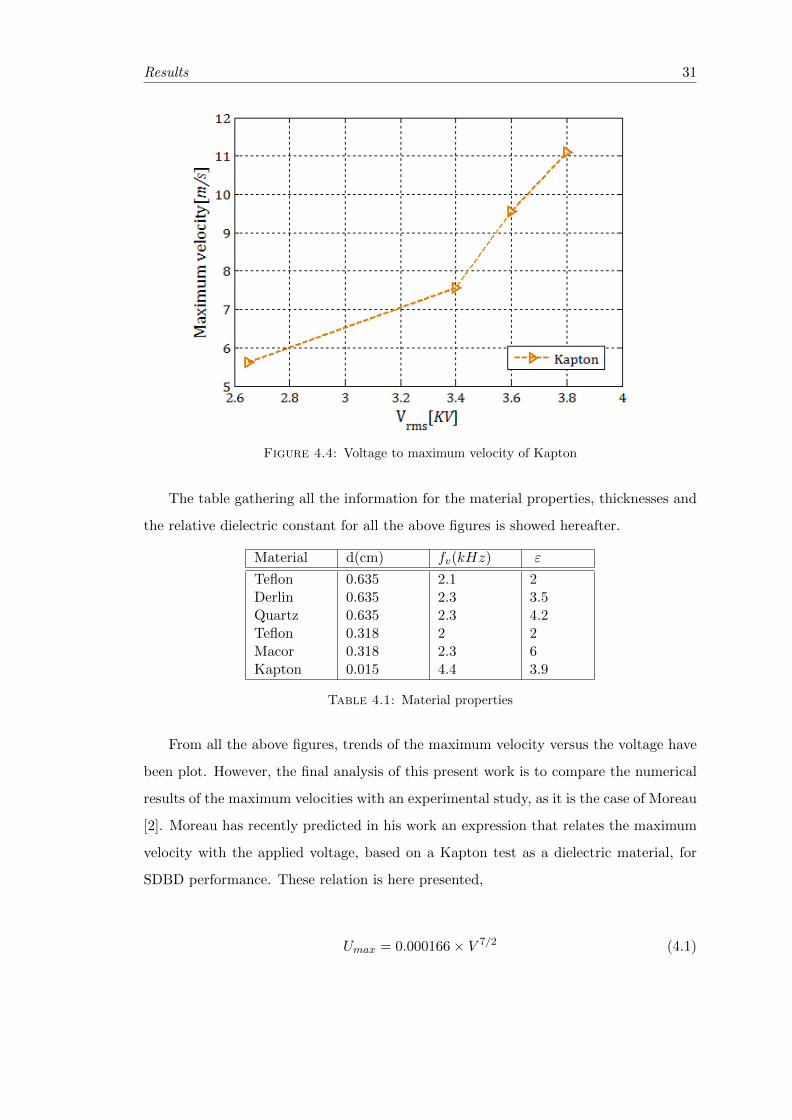
4.4 Voltage to maximum velocity of Kapton . . . . . . . . . . . . . . . . . . . 31

4.5 Moreau estimation of the Vmax relation with voltage applied using Kap-ton as dielectric material [2] . . . . . . . . . . . . . . . . . . . . . . . . . . 32

4.6 Experimental data versus numerical data for Kapton . . . . . . . . . . . . 32

A.1 Integration limits . . . . . . . . . . . . . . . . . . . . . . . . . . . . . . . . 39

A.2 Integration limits . . . . . . . . . . . . . . . . . . . . . . . . . . . . . . . . 39

List of Tables

2.1 Material properties . . . . . . . . . . . . . . . . . . . . . . . . . . . . . . . 8

4.1 Material properties . . . . . . . . . . . . . . . . . . . . . . . . . . . . . . . 31

5.1 Cost estimation . . . . . . . . . . . . . . . . . . . . . . . . . . . . . . . . . 35

A.1 Force values . . . . . . . . . . . . . . . . . . . . . . . . . . . . . . . . . . . 39

vi

Abbreviations

AC Alternate Current

CFD Computational Fluid Dynamics

DBD Dielectric Barrier Discharge

EHD Electro Hydrodimanic Dynamic

MAV User Arial Vehicle

RF Radio Frequency

SDBD Surface Dielectric Barrier Discharge

UAV Unnamed Arial Vehicle

UDF User Define Function

vii

Chapter 1

Introduction

Boundary layer control has led to several discussions within the aerodynamic scope.

Many related issues regarding flow separation are of interest due to its detrimental

consequences. Well-known associated problems such as buffet have to do with this

phenomenon. Nevertheless, flow control extents not only to airfoil flow control but also

to any airflow in general such as internal aerodynamics (ducts or diffusers), internal and

external blades or other flying bodies, UAV and MAV, among others.

Todays methods for airfoil boundary layer control can be divided in two main cat-

egories of solutions. The first category corresponds to the group that gathers passive

methods, whereas the second category deals with active methods, like flapping wings or

methods based on Micro Electro Mechanical Systems and Electrohydronamic Actuators

(EHD), which transform electrical into mechanical power. These kind of actuators built

on this principle are the so-called plasma actuators, ranging from corona discharges and

electric barrier discharges (DBDs), glow discharges and arc discharges.

The most employed active controls in the Aeronautical Industry are typically parts

integrated into the airfoil, modifying the lifting surface. The moving mechanical parts

are known as flaps and slats. Moving parts are the main cause of vibrational and acoustic

problems, such as control reversals, divergence or flutter; severe aeroeleastic problems

associated to the controls of the lifting surfaces.

An alternative to moving mechanisms is the use of active controls based on plasma

actuators, which have been tremendously investigated during the last decade. Plasma

actuators demonstrate their potential for flow control at the leading edge or centre of

1

Introduction 2

the airfoil, inducing significant the attachment and detachment of the boundary layer,

without the addition of mechanical parts. The application of DBD on other bodies such

as cylinders have led to the suppression of the global instability and the vortex shedding

for different Reynolds range.

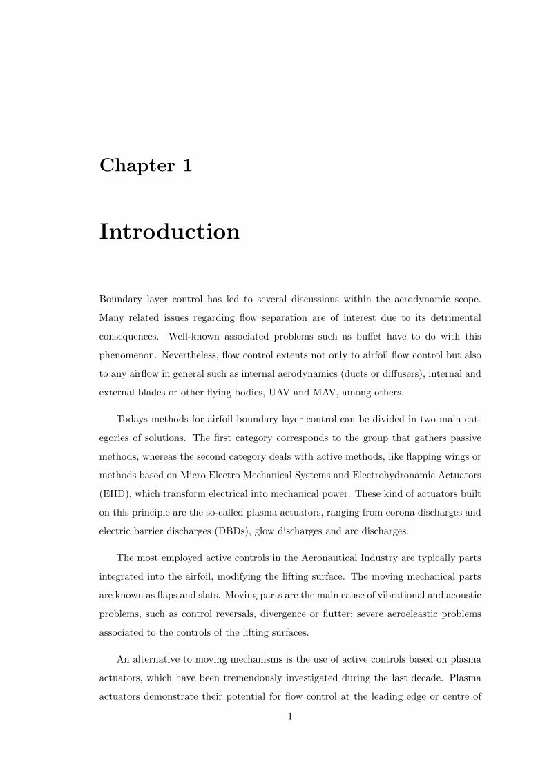
Several experimental tests have been performed over these bodies with smoke visu-

alizations providing a better physical understanding of the plasma effect on boundary

layer mitigation [2] [3]. The reader is encouraged to see the addressed references in the

literature.

Figure 1.1: Plasma actuator over an airfoil

Figure 1.2: Plasma actuator over a cylinder

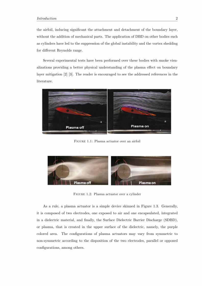
As a rule, a plasma actuator is a simple device skinned in Figure 1.3. Generally,

it is composed of two electrodes, one exposed to air and one encapsulated, integrated

in a dielectric material, and finally, the Surface Dielectric Barrier Discharge (SDBD),

or plasma, that is created in the upper surface of the dielectric, namely, the purple

colored area. The configurations of plasma actuators may vary from symmetric to

non-symmetric according to the disposition of the two electrodes, parallel or opposed

configurations, among others.

Introduction 3

Figure 1.3: SDBD configuration

Plasma airflow actuation mechanism is based on momentum transfer to the sur-

rounding air by means of collisions of the produced ions during the electrical discharges

(plasma) with the surrounding air particles. The result is an electrodynamic force,

thrust, that pushes the fluid in the neighborhood of the discharged region.

The advantages of Plasma Actuators for airflow control are the suppression of moving

mechanical parts and the high time response. Several experiments, [4], have shown

its efficient performance to reattachment at high angles of attack; yet, limited by the

Reynolds number. Besides, the cost of the setting is low due to the easy schematic and

the materials required that lead to an easy manufacturing.

Surface Dielectric Barrier Discharge (SDBD), or plasma, is a complex medium con-

taining neutral spices electron and ion interaction through collision and with a self-

consistent electric field. Because the prediction of the thrust generated by a DBD and

its effect on airflow is far from trivial (necessity of coupling the Navier-Stokes equations

with Poisson equations and the kinematics) for systematic calculations, it is better to

model the effect of the DBD actuator in a simple body source term that can be eas-

ily implemented into commercial CFD solver. With this simple model, engineers can

play with the source term for the study of the aerodynamic performance of different

applications, such as boundary control.

All in all, the primary objective of this paper is to represent the thrust generated

by a surface dielectric barrier discharge (SDBD) in a new force model form, in order to

implement it in a CFD solver, as it is the case of Fluent. The heritage of this paper is two

main studies where the distribution of the force of a plasma actuator is approximated,

and a second one, where the absolute value of the thrust of plasma actuators has been

calculated.

Introduction 4

Starting from scratch, this paper is divided in different chapters. Initially the state of

the art and the selected geometry of the plasma actuator is specifically defined, followed

by the description of the two models of interest that are the bases to build the new model

of force. Once the third model of force is built, a preliminary assessment on a CFD solver,

Fluent, will be performed for the three addressed models. The numerical assessment

has been the main task of the project in order to provide an accurate simulation of the

velocity vector profiles and velocity magnitude for the force models, lasting two months

for the developments of all the calculations. Finally, analysis of the results is gathered

at the end.

Two-dimensional modeling is assumed to be a good approach for all the forces,

as long as, it perfectly allows the simulation of the SDBD evolution, as well as, the

simplifications in calculations that it entails. The work is modeled to a mechanical point

of view, neglecting the complexity of the physics of the plasma, yet with a formulation

compliant with the plasma physics.

Chapter 2

SDBD models of force

2.1 Description of the model

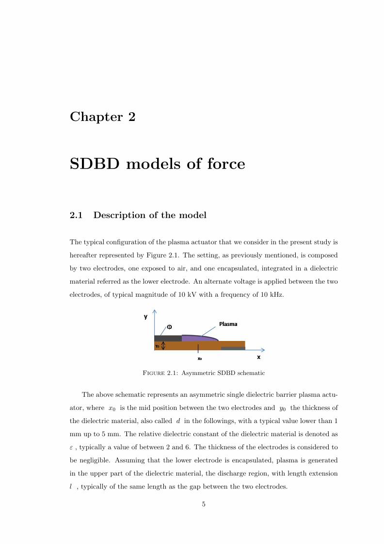
The typical configuration of the plasma actuator that we consider in the present study is

hereafter represented by Figure 2.1. The setting, as previously mentioned, is composed

by two electrodes, one exposed to air, and one encapsulated, integrated in a dielectric

material referred as the lower electrode. An alternate voltage is applied between the two

electrodes, of typical magnitude of 10 kV with a frequency of 10 kHz.

Figure 2.1: Asymmetric SDBD schematic

The above schematic represents an asymmetric single dielectric barrier plasma actu-

ator, where x0 is the mid position between the two electrodes and y0 the thickness of

the dielectric material, also called d in the followings, with a typical value lower than 1

mm up to 5 mm. The relative dielectric constant of the dielectric material is denoted as

ε , typically a value of between 2 and 6. The thickness of the electrodes is considered to

be negligible. Assuming that the lower electrode is encapsulated, plasma is generated

in the upper part of the dielectric material, the discharge region, with length extension

l , typically of the same length as the gap between the two electrodes.

5

Models of force 6

Rigorously, the momentum transfer from the plasma to the surrounding air is due

to the acceleration of ions in both directions depending on the applied voltage. The

generation of thrust with DBD plasma actuator is a complex phenomena that involves

momentum transfers at microscopic scale that can be schematized as following:

The electron accelerated in the electric field dissociate and ionize the neutral species

of air (O2, N2), then positive ions are accelerated in the electric field and collides with

neutral species (which are insensitive to the electric field), and transfers their kinetic en-

ergy through individual collisions leading to the generation of directed thrust observable

at macroscopic scale.

For the proper modeling of plasma actuators, continuity equations need to be solved

for different species, Poissons Equation, and Navier-Stokes equations self-consistently.

Previous studies solving these equations have lead to different formulations (see [1],

Section I. This procedure is a time consuming task and rather expensive.

Figure 2.2: Momentum tranfer

From an engineering point of view, the generated thrust can be approximated as a

steady momentum force, where a thrust pushes the air in one direction, depending on

the configuration of the actuator, which for the schematic in 2.1. pushes the fluid to the

right. In this way, the plasma physics are reduced to a mechanical problem, effective

for the methodology of this study. In the followings, the plasma actuator is operating

in atmospheric air.

Figure 2.3: Steady thrust approximation

Focusing on the methodologies of this work, the heritage of this study is two ap-

proximated models of force: the global thrust model by by V R Soloviev [5] and local

Models of force 7

thrust model by Singh et al. [1]. The former model predicts the total amount of gen-

erated thrust by the actuator [5] whereas the latter describes the local thrust density

distribution generated by the actuator.

Each model will be explained in the forthcoming sections and the third model will

be built at the end on the bases of the two addressed models.

2.2 Global thrust model

V R Soloviev [5] has recently obtained an analytical estimation of the integral value of

the body force (thrust) of a SDBD. His main driver to work on it was the understanding

of the saturation effect that is produced in the actuator. Additionally, the expression

obtained by V R Soloviev provides a direct relation between the voltage parameter and

the dielectric material properties on the performance of the plasma actuator.

The integration of the body force over space and its averaging over time, give thrust

per unit electrode length equal to:

Thrust =1

TV

∫ Tv

0

∫ −∞∞

∫ ∞0

f(t, x, y)dtdxdy (2.1)

Where TV is the period of the applied voltage.

By substituting and integrating this last expression the final thrust generated by

SDBD is retrieved. Nevertheless, a thorough substitution of the value of each parameter

that composes the integral is carried out in [5]. The final expression is showed and

hereafter plotted.

Tsol = 2.4× 10−10αl4 fV (cm)

d(kHz)

(9V0

4∆Vc

)4(1− 7∆Vc

6V0

)4(1− exp

(− 1

4fv∆τq

))(2.2)

Where αl = 1,∆Vc = 0.6kV,∆τq = 100 × 10−6 seconds, values taken from [5],

following his recommendations. Moreover fV is the frequency, d corresponds to the

thickness of the material and V0 is the voltage applied.

Models of force 8

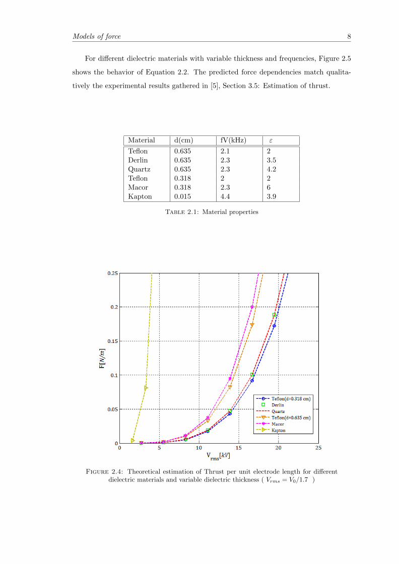
For different dielectric materials with variable thickness and frequencies, Figure 2.5

shows the behavior of Equation 2.2. The predicted force dependencies match qualita-

tively the experimental results gathered in [5], Section 3.5: Estimation of thrust.

Material d(cm) fV(kHz) ε

Teflon 0.635 2.1 2Derlin 0.635 2.3 3.5Quartz 0.635 2.3 4.2Teflon 0.318 2 2Macor 0.318 2.3 6Kapton 0.015 4.4 3.9

Table 2.1: Material properties

Figure 2.4: Theoretical estimation of Thrust per unit electrode length for differentdielectric materials and variable dielectric thickness ( Vrms = V0/1.7 )

Models of force 9

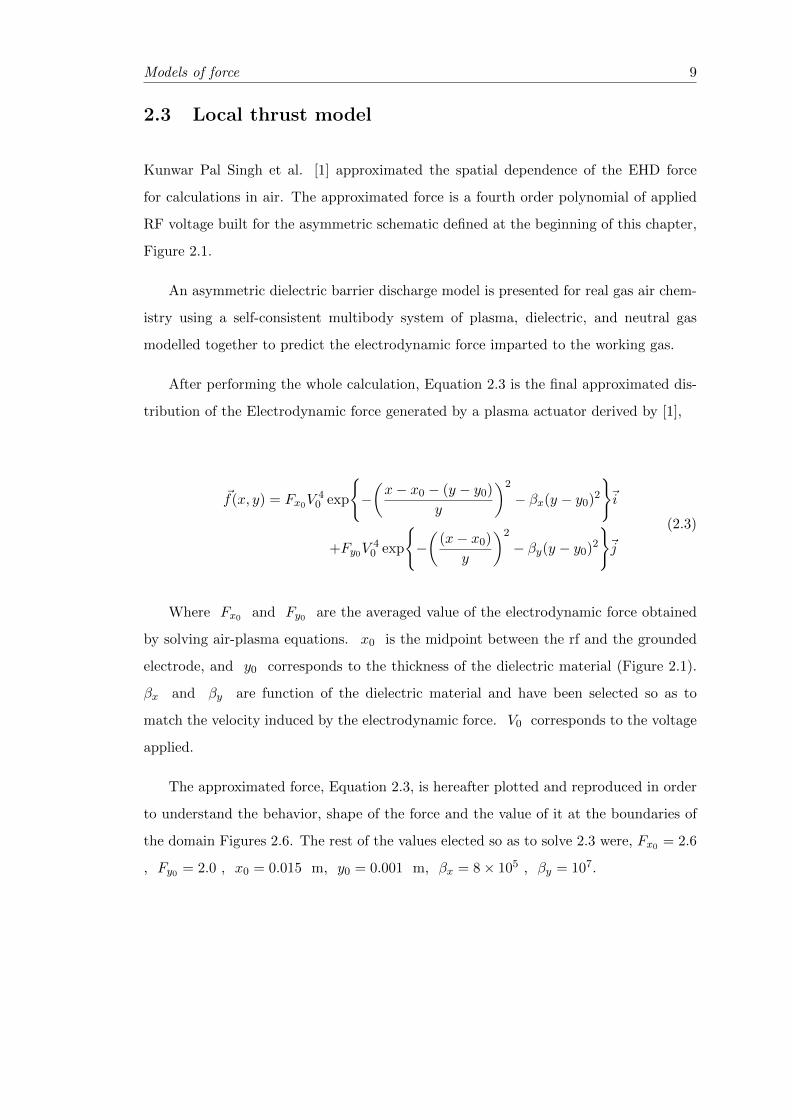
2.3 Local thrust model

Kunwar Pal Singh et al. [1] approximated the spatial dependence of the EHD force

for calculations in air. The approximated force is a fourth order polynomial of applied

RF voltage built for the asymmetric schematic defined at the beginning of this chapter,

Figure 2.1.

An asymmetric dielectric barrier discharge model is presented for real gas air chem-

istry using a self-consistent multibody system of plasma, dielectric, and neutral gas

modelled together to predict the electrodynamic force imparted to the working gas.

After performing the whole calculation, Equation 2.3 is the final approximated dis-

tribution of the Electrodynamic force generated by a plasma actuator derived by [1],

~f(x, y) = Fx0V40 exp

{−(x− x0 − (y − y0)

y

)2

− βx(y − y0)2}~i

+Fy0V40 exp

{−(

(x− x0)y

)2

− βy(y − y0)2}~j

(2.3)

Where Fx0 and Fy0 are the averaged value of the electrodynamic force obtained

by solving air-plasma equations. x0 is the midpoint between the rf and the grounded

electrode, and y0 corresponds to the thickness of the dielectric material (Figure 2.1).

βx and βy are function of the dielectric material and have been selected so as to

match the velocity induced by the electrodynamic force. V0 corresponds to the voltage

applied.

The approximated force, Equation 2.3, is hereafter plotted and reproduced in order

to understand the behavior, shape of the force and the value of it at the boundaries of

the domain Figures 2.6. The rest of the values elected so as to solve 2.3 were, Fx0 = 2.6

, Fy0 = 2.0 , x0 = 0.015 m, y0 = 0.001 m, βx = 8× 105 , βy = 107.

Models of force 10

Figure 2.5: 2D and XY plots of the distributed force. Left figures for the Fx compo-nent and right figures for Fy component of the force.

The force is concentrated in the reference point of the actuator, for the plotted figures

at 0.015 m in the x-axis, tending to zero for the limits of the domain. According to this,

the pressure at those limits is equal to the ambient pressure. The air is stationary,

quiescent, with density of 1.225 Kg/m3.

Models of force 11

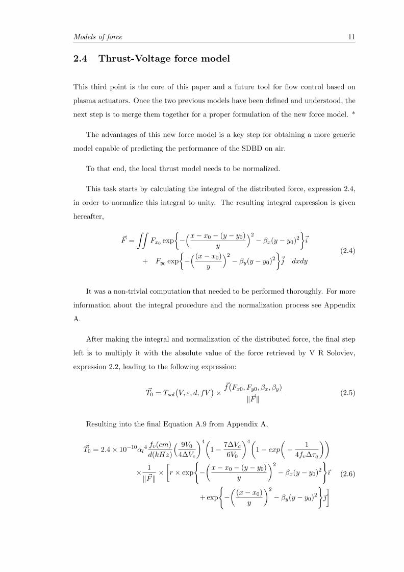
2.4 Thrust-Voltage force model

This third point is the core of this paper and a future tool for flow control based on

plasma actuators. Once the two previous models have been defined and understood, the

next step is to merge them together for a proper formulation of the new force model. *

The advantages of this new force model is a key step for obtaining a more generic

model capable of predicting the performance of the SDBD on air.

To that end, the local thrust model needs to be normalized.

This task starts by calculating the integral of the distributed force, expression 2.4,

in order to normalize this integral to unity. The resulting integral expression is given

hereafter,

~F =

∫∫Fx0 exp

{−(x− x0 − (y − y0)

y

)2− βx(y − y0)2

}~i

+ Fy0 exp

{−((x− x0)

y

)2− βy(y − y0)2

}~j dxdy

(2.4)

It was a non-trivial computation that needed to be performed thoroughly. For more

information about the integral procedure and the normalization process see Appendix

A.

After making the integral and normalization of the distributed force, the final step

left is to multiply it with the absolute value of the force retrieved by V R Soloviev,

expression 2.2, leading to the following expression:

~T0 = Tsol(V, ε, d, fV

)×~f(Fx0, Fy0, βx, βy)

‖~F‖(2.5)

Resulting into the final Equation A.9 from Appendix A,

~T0 = 2.4× 10−10αl4 fv(cm)

d(kHz)

( 9V04∆Vc

)4(1− 7∆Vc

6V0

)4(1− exp

(− 1

4fv∆τq

))× 1

‖~F‖×[r × exp

{−(x− x0 − (y − y0)

y

)2

− βx(y − y0)2}~ı

+ exp

{−(

(x− x0)y

)2

− βy(y − y0)2}~

] (2.6)

Models of force 12

Clearly, the advantages of this new model outweigh the disadvantages of the other

two, as it is the combination of both in order to provide an improved version. The

new expression of force depends only on the voltage applied, the dielectric material, and

thickness of the dielectric material, and frequency which allows an easy configuration

and parametric study.

F (V, ε, d, fV )

On the other hand, the integral expression still contains two more variables coming

from the local thrust model, βx, βy, Fx0 , Fy0 . The last two terms appear also in form

of a ratio, namely, r :

r =Fx0

Fy0

(2.7)

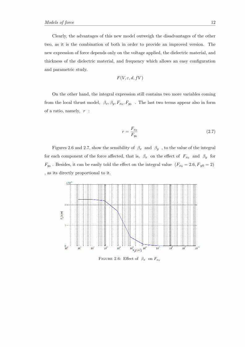
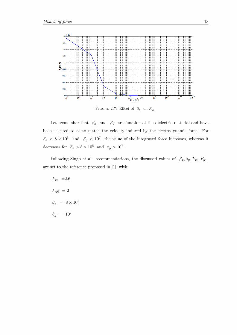
Figures 2.6 and 2.7, show the sensibility of βx and βy , to the value of the integral

for each component of the force affected, that is, βx on the effect of Fx0 and βy for

Fy0 . Besides, it can be easily told the effect on the integral value (Fx0 = 2.6, F y0 = 2)

, as its directly proportional to it.

Figure 2.6: Effect of βx on Fx0

Models of force 13

Figure 2.7: Effect of βy on Fy0

Lets remember that βx and βy are function of the dielectric material and have

been selected so as to match the velocity induced by the electrodynamic force. For

βx < 8 × 105 and βy < 107 the value of the integrated force increases, whereas it

decreases for βx > 8× 105 and βy > 107 .

Following Singh et al. recommendations, the discussed values of βx, βy, Fx0 , Fy0

are set to the reference proposed in [1], with:

Fx0 =2.6

F y0 = 2

βx = 8× 105

βy = 107

Chapter 3

Assessment in CFD solver: Fluent

3.1 Fluent framework

Computational Fluid Dynamics programs have the characteristic of solving Naiver-

Stokes equations for any kind of fluid flow in a quantitative version of the results,

namely, a numerical solution. The great advantage of CFD is that they can handle

any kind of continuity, momentum and energy equation for several problems limited for

the analytical scope.

The working principle of CFD is that the continuity, momentum, and energy equa-

tions are discretized. In order to do so, the flow domain is divided into a number of

discrete points. A grid is generated and the discrete points are converted into grid

points. There are many basis for dicretization, however, the basic principle is showed

below, where the scripts of the grid points are defined:

Figure 3.1: Grid points

14

Assessment in CFD solver 15

For any differential or integral form, the equations are substituted and calculated

iteratively for each point by means of substituting the points with the subscripts. For

more information about the discretization process see [6], Chapter 2, section 17.

For the purpose of this paper, Fluent has been the computational software selected

due to its availability at the Aerospace Engineering Department of Carlos III University.

Fluent, among other features, allows the direct implementation of a source term in the

Navier-Stokes momentum equations.

As regarded in Chapter 2, three models of force have been addressed; models, that

indeed, need to be implemented in the momentum equations in order to solve the inter-

actions between the plasma physics and the quiescent air, which surrounds the plasma.

From a mathematical point of view, the force models are implemented with an specific

User Define Function (UDF), programed in C, into Fluent, adding the corresponding

source term into the Navier-Sotkes Equations:

∂ρ

∂t+∂(ρui)

∂xi= 0 (3.1)

∂(ρui)

∂t+∂(ρuiuj)

∂xj= − ∂p

∂xi+∂τij∂xj

+ ρfi (3.2)

∂(ρe)

∂t+ (ρe+ p)

∂ui∂xi

=∂(τijuj)

∂xi+ ρfiui +

∂(qi)

∂xi+ r (3.3)

In classic notation,

~∇ · (ρ~u) = 0 (3.4)

∂(ρ~u)

∂t+ ~∇ · ρ~u⊗ ~u = − ~∇p+ ~∇ · ¯τ + ρ~f (3.5)

∂(ρe)

∂t+ ~∇ · (ρe+ p)~u = ~∇ · (¯τ · ~u) + ρ~f~u+ ~∇ · ~q + r (3.6)

In the momentum equations, 3.2 and 3.5, the source terms are defined and imple-

mented in the fi or, in the classic notation, ~f , components.

As far as the aim of this paper is concerned, a variety of simulations in Fluent of

the models of force is performed in order to obtain the velocity vector profiles of the

surrounding air when plasma is activated.

Assessment in CFD solver 16

On top of that, the general Fluent methodology is hereafter introduced:

• Preprocessing

1. A geometry domain is set with the tool Design Modeler. The selected domain is

a rectangular, two dimensional. The dimensions of the domain are 0.03 m long and 0.01

m high.

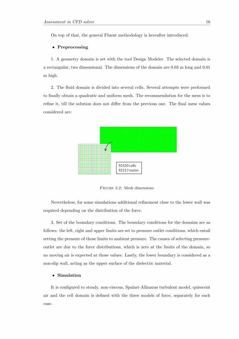
2. The fluid domain is divided into several cells. Several attempts were performed

to finally obtain a quadratic and uniform mesh. The recommendation for the mess is to

refine it, till the solution does not differ from the previous one. The final mess values

considered are:

Figure 3.2: Mesh dimensions

Nevertheless, for some simulations additional refinement close to the lower wall was

required depending on the distribution of the force.

3. Set of the boundary conditions. The boundary conditions for the domains are as

follows: the left, right and upper limits are set to pressure outlet conditions, which entail

setting the pressure of those limits to ambient pressure. The causes of selecting pressure-

outlet are due to the force distributions, which is zero at the limits of the domain, so

no moving air is expected at those values. Lastly, the lower boundary is considered as a

non-slip wall, acting as the upper surface of the dielectric material.

• Simulation

It is configured to steady, non-viscous, Spalart-Allmaras turbulent model, quiescent

air and the cell domain is defined with the three models of force, separately for each

case.

Assessment in CFD solver 17

Preliminary simulations were performed in laminar flow, with no success in terms of

convergence of the solution. This led to the use of the Spalart-Allmaras model, which

is a turbulent viscous model specifically recommended for wall-bounded flows. It is

generally use for aerospace applications, and it worked for the simulations carried out

in the current paper.

The simulation is solved iteratively till the solution is converged. After each iteration,

the residual sum of each variable is calculated and stored, so it is created and recorded

a convergence history, which can be visualized in the monitors.

• Post-processing

The post-processing allows displaying the results. Vectors, contours, XY plots are

configured to visualize the outcome of the simulation.

3.2 Global thrust model assessment

Reproduction of the V. R. Soloviev, [5], global thrust model in a Fluent simulation is

performed. To that end, arbitrary body force distributions are selected, on intuition

of the local distribution of the EHD force. The two distributions are two Gaussian

distributions and one rectangular distribution.

The arbitrary distributions times the thrust defined in Equation 2.2 is implemented

in fluent. The total thrust selected for the calculation is 0.1 N/m, from the global thrust

model, Figure 2.5.

a) 2D Gaussian distribution, of the form:

g(x, y) = A× exp[−(

(x− x0)2

2σ2x+

(y − y0)2

2σ2y

)](3.7)

where x0 = 0.015 m and y0 = 0.001 m. A is the normalization factor,

A =1

πσxσy(3.8)

and σx and σy determine the shape to the Gaussian distribution. Two different sigma

values, shapes of the Gaussian, are considered:

Assessment in CFD solver 18

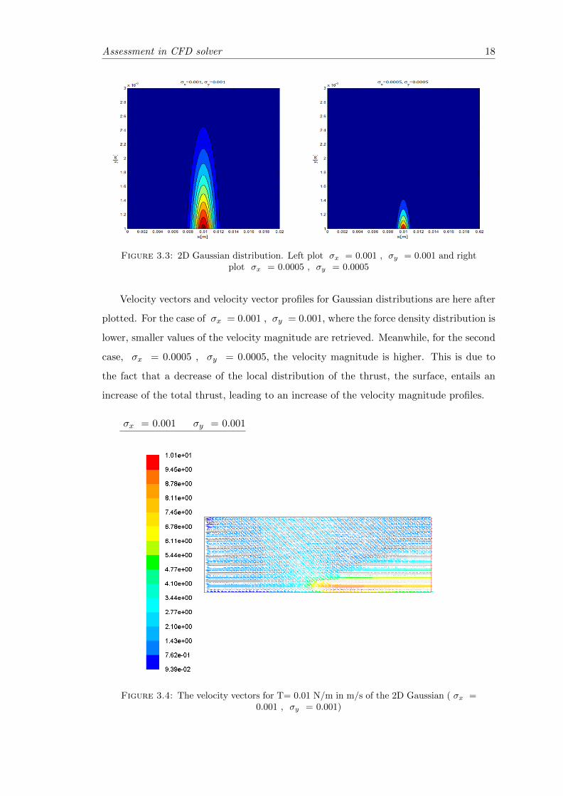
Figure 3.3: 2D Gaussian distribution. Left plot σx = 0.001 , σy = 0.001 and rightplot σx = 0.0005 , σy = 0.0005

Velocity vectors and velocity vector profiles for Gaussian distributions are here after

plotted. For the case of σx = 0.001 , σy = 0.001, where the force density distribution is

lower, smaller values of the velocity magnitude are retrieved. Meanwhile, for the second

case, σx = 0.0005 , σy = 0.0005, the velocity magnitude is higher. This is due to

the fact that a decrease of the local distribution of the thrust, the surface, entails an

increase of the total thrust, leading to an increase of the velocity magnitude profiles.

σx = 0.001 σy = 0.001

Figure 3.4: The velocity vectors for T= 0.01 N/m in m/s of the 2D Gaussian ( σx =0.001 , σy = 0.001)

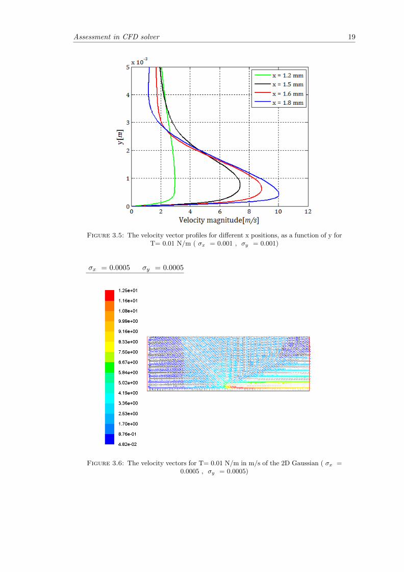
Assessment in CFD solver 19

Figure 3.5: The velocity vector profiles for different x positions, as a function of y forT= 0.01 N/m ( σx = 0.001 , σy = 0.001)

σx = 0.0005 σy = 0.0005

Figure 3.6: The velocity vectors for T= 0.01 N/m in m/s of the 2D Gaussian ( σx =0.0005 , σy = 0.0005)

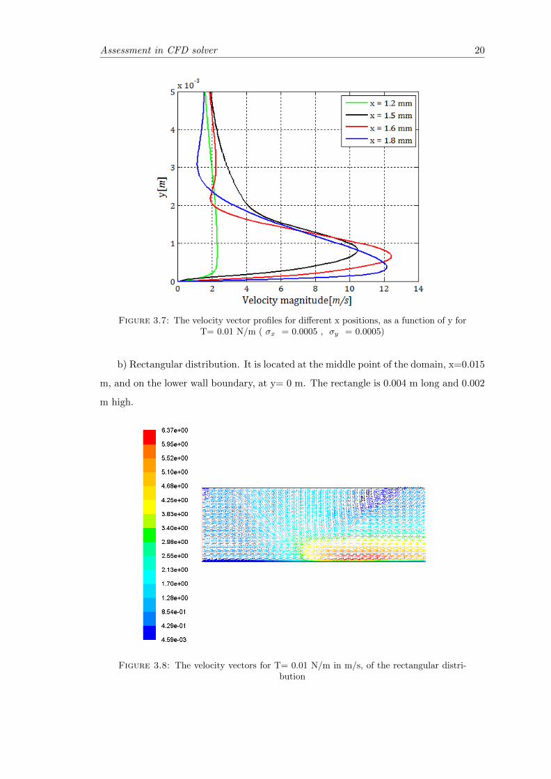
Assessment in CFD solver 20

Figure 3.7: The velocity vector profiles for different x positions, as a function of y forT= 0.01 N/m ( σx = 0.0005 , σy = 0.0005)

b) Rectangular distribution. It is located at the middle point of the domain, x=0.015

m, and on the lower wall boundary, at y= 0 m. The rectangle is 0.004 m long and 0.002

m high.

Figure 3.8: The velocity vectors for T= 0.01 N/m in m/s, of the rectangular distri-bution

Assessment in CFD solver 21

Figure 3.9: The velocity vector profiles for three x positions, as a function of y forT= 0.01 N/m, of the rectangular distribution

Comparing the velocity vector profiles of the rectangular distribution with those of

the Gaussian distributions, it can be directly noticed that the resulting velocity profiles in

terms of morphology are strongly different from the ones reproduced with the Gaussian.

On the other hand, differences in the velocity magnitude can be found, yet with similar

order of magnitude close to the experimental values for SDBD.

These results lead to an important fact that should be pointed out. The work re-

produced by Soloviev [5] provides a valuable numerical estimation of the total thrust,

however, there is no information about the distribution of the local EHD. Therefore,

a model with the distribution of the local force is required in order to provide a com-

plete force model. Otherwise, random distributions can be sketched following intuition.

However, as we have shown for the square and the Gaussian distributions, the resulting

velocity profiles can vary from 6 to 12 m/s.

The same remark can be done regarding the model of Singh [1] which predicts the

distribution but does not predict the total thrust.

Assessment in CFD solver 22

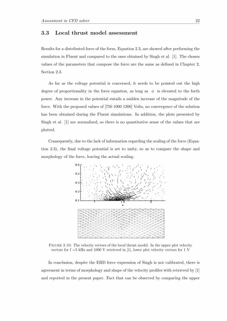
3.3 Local thrust model assessment

Results for a distributed force of the form, Equation 2.3, are showed after performing the

simulation in Fluent and compared to the ones obtained by Singh et al. [1]. The chosen

values of the parameters that compose the force are the same as defined in Chapter 2,

Section 2.3.

As far as the voltage potential is concerned, it needs to be pointed out the high

degree of proportionality in the force equation, as long as φ is elevated to the forth

power. Any increase in the potential entails a sudden increase of the magnitude of the

force. With the proposed values of [750 1000 1200] Volts, no convergence of the solution

has been obtained during the Fluent simulations. In addition, the plots presented by

Singh et al. [1] are normalized, so there is no quantitative sense of the values that are

plotted.

Consequently, due to the lack of information regarding the scaling of the force (Equa-

tion 2.3), the final voltage potential is set to unity, so as to compare the shape and

morphology of the force, leaving the actual scaling.

Figure 3.10: The velocity vectors of the local thrust model. In the upper plot velocityvectors for f =5 kHz and 1000 V retrieved in [1], lower plot velocity vectors for 1 V

In conclusion, despite the EHD force expression of Singh is not calibrated, there is

agreement in terms of morphology and shape of the velocity profiles with retrieved by [1]

and reported in the present paper. Fact that can be observed by comparing the upper

Assessment in CFD solver 23

plots of Singh et al. [1] of Figure 3.10 and Figure 3.11, with the lower plots retrieved in

the present work of the same figures for 1V.

Figure 3.11: The normalized velocity components as a function of y for differentlocations of x, in the upper plot velocity vectors for f =5 kHz and 1000 V retrieved in

[1], lower plot velocity vectors for 1 V

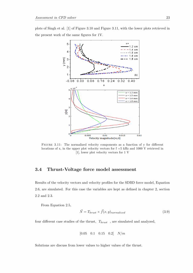
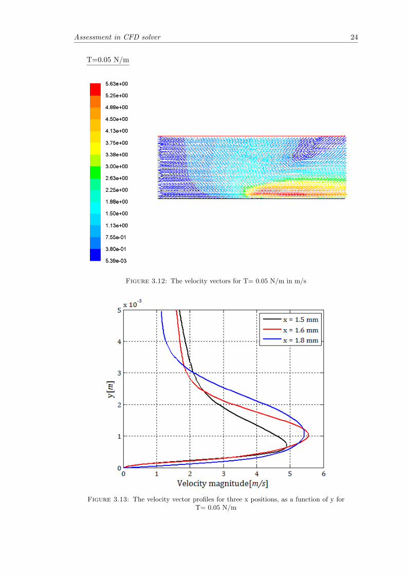
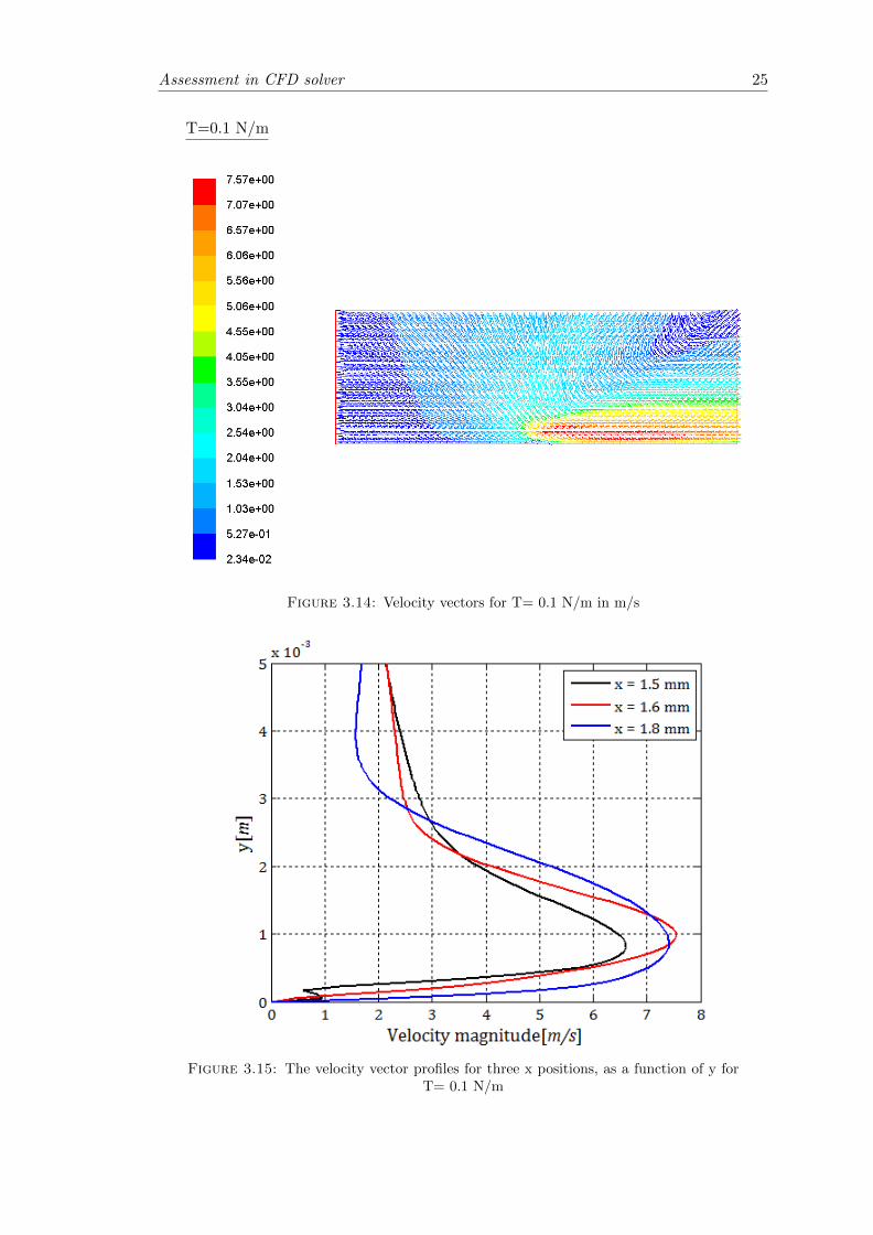
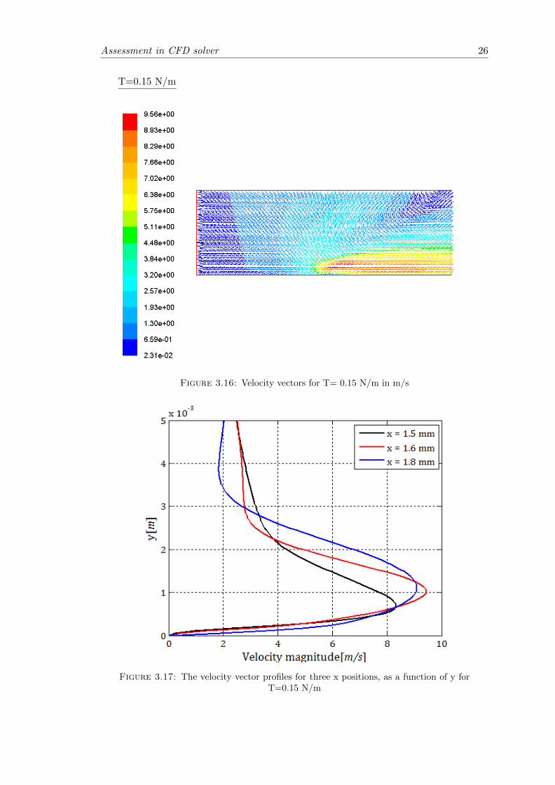
3.4 Thrust-Voltage force model assessment

Results of the velocity vectors and velocity profiles for the SDBD force model, Equation

2.6, are simulated. For this case the variables are kept as defined in chapter 2, section

2.2 and 2.3.

From Equation 2.5,

~N = Thrust × ~f(x, y)normalized (3.9)

four different case studies of the thrust, Thrust , are simulated and analyzed,

[0.05 0.1 0.15 0.2] N/m

Solutions are discuss from lower values to higher values of the thrust.

Assessment in CFD solver 24

T=0.05 N/m

Figure 3.12: The velocity vectors for T= 0.05 N/m in m/s

Figure 3.13: The velocity vector profiles for three x positions, as a function of y forT= 0.05 N/m

Assessment in CFD solver 25

T=0.1 N/m

Figure 3.14: Velocity vectors for T= 0.1 N/m in m/s

Figure 3.15: The velocity vector profiles for three x positions, as a function of y forT= 0.1 N/m

Assessment in CFD solver 26

T=0.15 N/m

Figure 3.16: Velocity vectors for T= 0.15 N/m in m/s

Figure 3.17: The velocity vector profiles for three x positions, as a function of y forT=0.15 N/m

Assessment in CFD solver 27

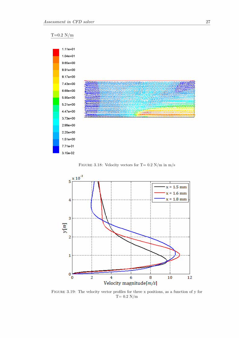
T=0.2 N/m

Figure 3.18: Velocity vectors for T= 0.2 N/m in m/s

Figure 3.19: The velocity vector profiles for three x positions, as a function of y forT= 0.2 N/m

Assessment in CFD solver 28

Linear trend of the above solutions is observed. For increasing thrust, the maximum

velocity increases too. In addition, there is concordance between the velocity profiles

retrieved for the Thrust-Voltage model and the Singh et al. [1] plots, Figure 3.11.

Two agreements can be stated:

• Morphologically agreement with Singh, [1].

• Quantitative agreement of the velocity magnitude with experimental data of [2].

Chapter 4

Voltage-Thrust force model

results

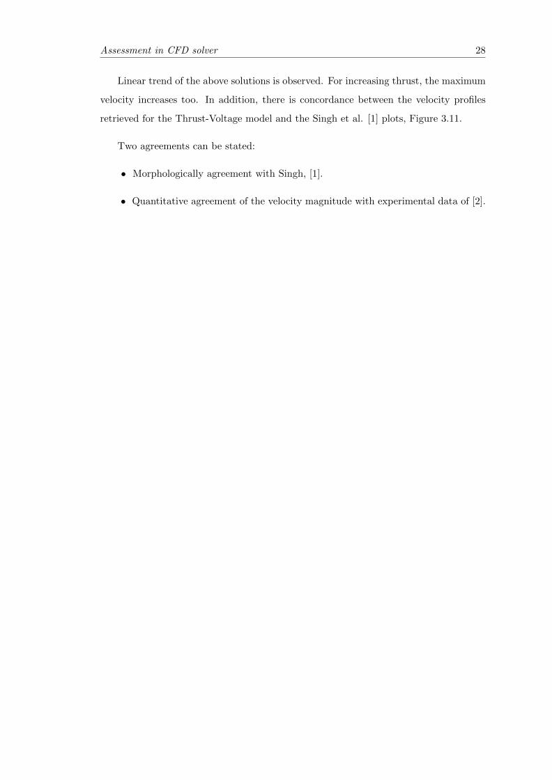
Section 3.4 gives a nice relationship between the voltage applied to an SDBD and the

velocity magnitude ranges of the surrounding air.

The linear trend noticed in the above section can be sketched resulting into Figure

4.1,

Figure 4.1: Thrust versus maximum velocity

In the light of the obtained results, not only the thrust-voltage relation can be

sketched, but also the relation between the voltage V0 and the maximum velocity that

can be achieved by an SDBD depending on the material properties and thicknesses.

29

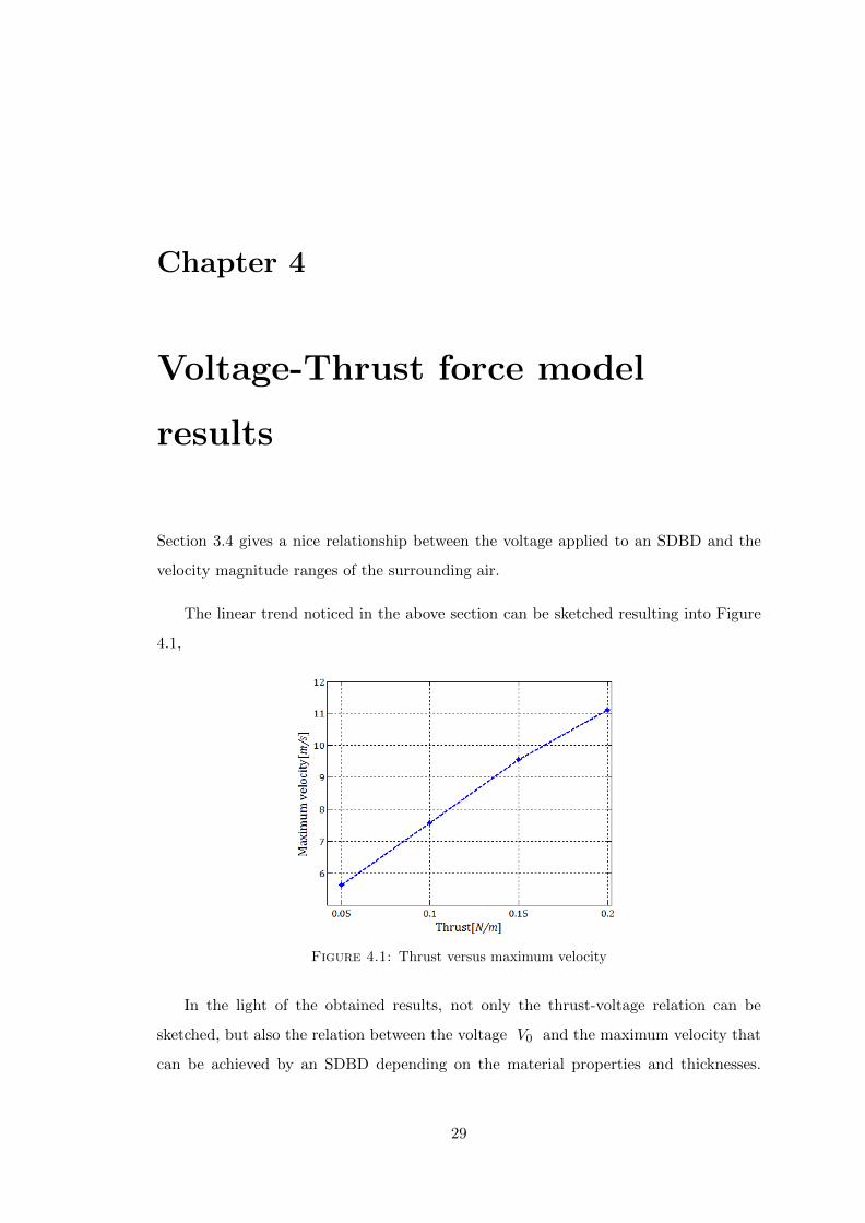
Results 30

This last relation comes from combining the Global Thrust model of V R soloviev [5],

Figure 2.5, with Figure 4.1, SDBD force model.

Figure 4.2: Voltage to maximum velocity of Teflon, Derlin and Quartz

Figure 4.3: Voltage to maximum velocity of Teflon and Macor

Results 31

Figure 4.4: Voltage to maximum velocity of Kapton

The table gathering all the information for the material properties, thicknesses and

the relative dielectric constant for all the above figures is showed hereafter.

Material d(cm) fv(kHz) ε

Teflon 0.635 2.1 2Derlin 0.635 2.3 3.5Quartz 0.635 2.3 4.2Teflon 0.318 2 2Macor 0.318 2.3 6Kapton 0.015 4.4 3.9

Table 4.1: Material properties

From all the above figures, trends of the maximum velocity versus the voltage have

been plot. However, the final analysis of this present work is to compare the numerical

results of the maximum velocities with an experimental study, as it is the case of Moreau

[2]. Moreau has recently predicted in his work an expression that relates the maximum

velocity with the applied voltage, based on a Kapton test as a dielectric material, for

SDBD performance. These relation is here presented,

Umax = 0.000166× V 7/2 (4.1)

Results 32

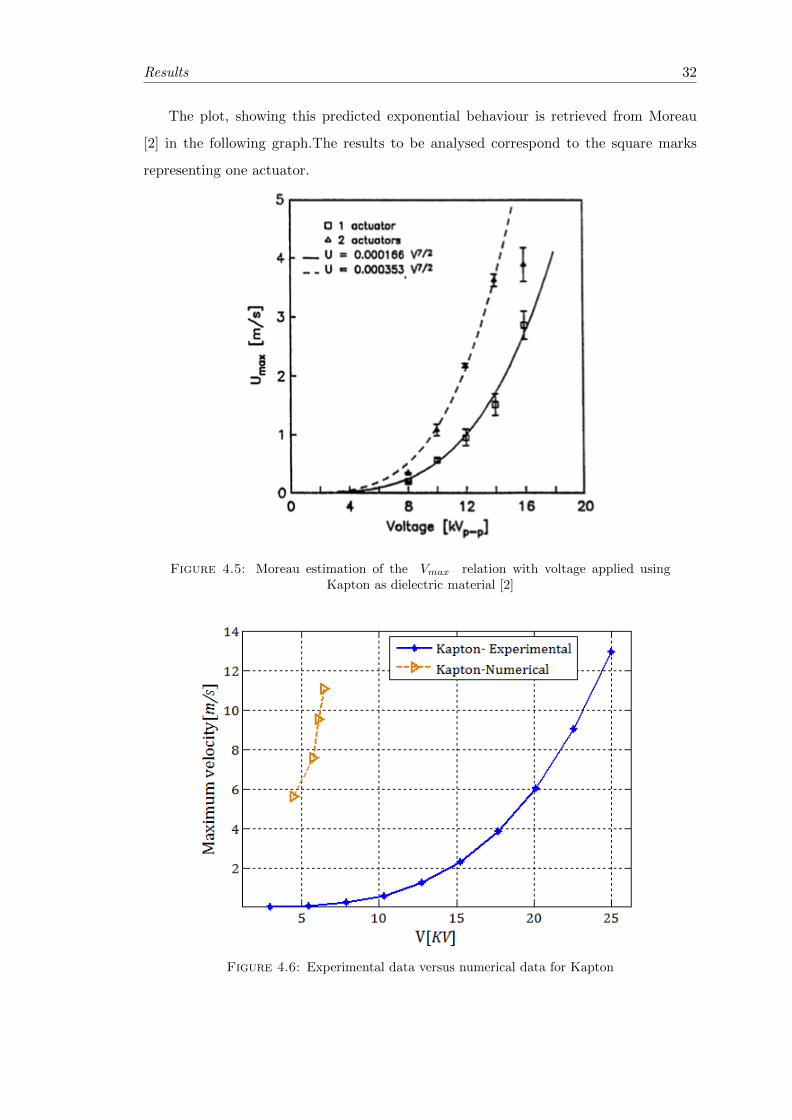
The plot, showing this predicted exponential behaviour is retrieved from Moreau

[2] in the following graph.The results to be analysed correspond to the square marks

representing one actuator.

Figure 4.5: Moreau estimation of the Vmax relation with voltage applied usingKapton as dielectric material [2]

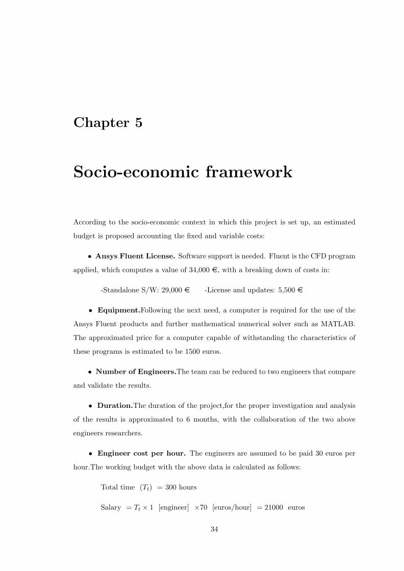
Figure 4.6: Experimental data versus numerical data for Kapton

Results 33

Comparison of the experimental results versus the numerical results of Kapton,

Figure 4.6, leads to a concordance in terms of trends of the relation Maximum velocity-

Voltage: increasing values of the maximum velocity for higher values of the voltage.

However, quantitatively speaking there is no agreement observed, yet within the same

order of magnitude. Some of the aspects that should be borne in mind for the differences

in the velocity magnitude is that Moreau does not specify the frequency used or the

voltage specification: V0 versus Vrms Moreover, in the Thrust- Voltage force model

negligible thickness of the electrodes is considered, whereas in [2] plays an important

role.

Chapter 5

Socio-economic framework

According to the socio-economic context in which this project is set up, an estimated

budget is proposed accounting the fixed and variable costs:

• Ansys Fluent License. Software support is needed. Fluent is the CFD program

applied, which computes a value of 34,000 e, with a breaking down of costs in:

-Standalone S/W: 29,000 e -License and updates: 5,500 e

• Equipment.Following the next need, a computer is required for the use of the

Ansys Fluent products and further mathematical numerical solver such as MATLAB.

The approximated price for a computer capable of withstanding the characteristics of

these programs is estimated to be 1500 euros.

• Number of Engineers.The team can be reduced to two engineers that compare

and validate the results.

• Duration.The duration of the project,for the proper investigation and analysis

of the results is approximated to 6 months, with the collaboration of the two above

engineers researchers.

• Engineer cost per hour. The engineers are assumed to be paid 30 euros per

hour.The working budget with the above data is calculated as follows:

Total time (Tt) = 300 hours

Salary = Tt × 1 [engineer] ×70 [euros/hour] = 21000 euros

34

Budget 35

• Expenditure. It amounts the variable costs of the electricity among others.

Finally,

Concept Amount (e)

Ansys Fluent package 34,000Equipment 1,500Salary 21,000Expenditure 300

TOTAL 56,800 e

Table 5.1: Cost estimation

On the other hand, the present project is in modeling phase therefore, no related

regulations should be addressed till the experimental set up is initiated. Nevertheless,

as far as future plasma complications are concerned, it is remarked the main issues that

should be taken into account:

• High voltage. High voltage operations need to be carefully controlled.

• Rf unsteady electromagnetic radiation. It can have a detrimental effect on the

near communication devices.

• Ozone production. This factor is important in the case the plasma actuator is

activated in a close room, as long as ozone is produced in a small proportion during the

electrical discharges.

Chapter 6

Conclusions

In the present work the force generated by an SDBD is modeled in to a body source

term that can be easily implemented into commercial CFD solver. The motivation

of this study is the complexity of the prediction of the thrust generated by a SDBD

and its effect on airflow (necessity of coupling the Navier-Stokes equations with Poisson

equations and the kinematics) for systematic calculations.

The performed theoretical and numerical calculations with two models of force:

global thrust model and local thrust model of a SDBD actuator has led to an interesting

force modeling, Thrust-Voltage force model , from an engineering point of view.

The main conclusions regarding the study performed in the present paper are here-

after drawn:

1. Final successful merge of the Soloviev [5] Global thrust model estimation and the

Singh et al.[1] Local thrust approximated model. The Thrust-Voltage model provides a

full description of the EHD force phenomena, from a qualitatively point of view, in terms

of morphology of the velocity profiles, with a proper prediction of the velocity vector

profiles, and from a quantitatively point view, in terms of magnitude of the velocity,

matching the same order of magnitude of the experimental results.

2. The direct relation between the thrust and the voltage of final SDBD body force

expression allows an easy study of the active parameters affecting the plasma actuator.

Nevertheless, it is recommended for future lines of study a deeper analysis of the variables

coming from the Singh force model, ~f(Fx0, Fy0, βx, βy) .

36

Conclusions 37

3. The Thrust-Voltage results on the effect of the maximum velocity have been

compared with experimental data of the same dielectric material (Kapton), provided in

[2], leading to two main conclusions. The magnitude of the maximum velocity retrieved

is higher, yet of the same order of magnitude. Further investigation on this difference

can be promising for approaching the model to more realistic data. Nevertheless, there

is concordance in terms of the trend of the plotted relation, with increasing velocity for

higher voltage.

4. The Voltage-Thrust model allows an easy implementation of the body force into

commercial CFD solver, providing time-cost saving in the resolution of problems with

SDBD involvement. The decrease of costs comes from the no need of manufacturing an

experimental set up for SDBD applications.

6.1 Future lines

Apart from the before mentioned improvements that can be performed to the Thrust-

Voltage model in order to approximate it to more realistic data, from this point, many

possibilities of study are opened within the aerodynamic scope.

The main driver to keep on working is for boundary layer control of aerodynamic

bodies such as UAV, MAV, blades, or airfoils, among others. Which will allow in the

future the removal of mechanical moving parts, main cause of vibrational and acoustic

problems.

It is left as a future case study, to perform a boundary layer detachment in a numer-

ical simulation and activate the plasma actuator, by means of implementing the body

force of the Thrust-Voltage model. Many geometries can be considered from flat plates

to NACA airfoil profiles.

Appendix A

Normalization of the local thrust

model

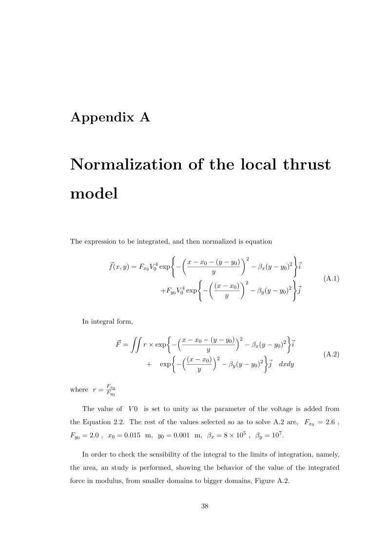
The expression to be integrated, and then normalized is equation

~f(x, y) = Fx0V40 exp

{−(x− x0 − (y − y0)

y

)2

− βx(y − y0)2}~i

+Fy0V40 exp

{−(

(x− x0)y

)2

− βy(y − y0)2}~j

(A.1)

In integral form,

~F =

∫∫r × exp

{−(x− x0 − (y − y0)

y

)2− βx(y − y0)2

}~i

+ exp

{−((x− x0)

y

)2− βy(y − y0)2

}~j dxdy

(A.2)

where r =Fx0Fy0

The value of V 0 is set to unity as the parameter of the voltage is added from

the Equation 2.2. The rest of the values selected so as to solve A.2 are, Fx0 = 2.6 ,

Fy0 = 2.0 , x0 = 0.015 m, y0 = 0.001 m, βx = 8× 105 , βy = 107.

In order to check the sensibility of the integral to the limits of integration, namely,

the area, an study is performed, showing the behavior of the value of the integrated

force in modulus, from smaller domains to bigger domains, Figure A.2.

38

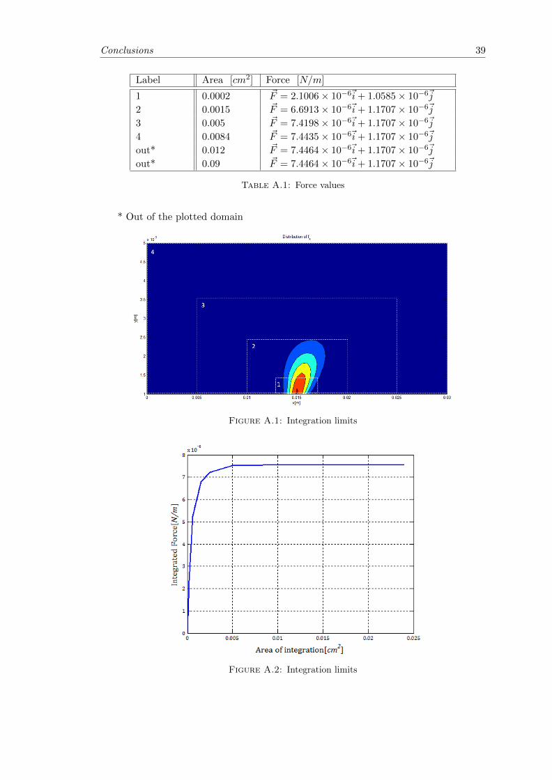
Conclusions 39

Label Area [cm2] Force [N/m]

1 0.0002 ~F = 2.1006× 10−6~i+ 1.0585× 10−6~j

2 0.0015 ~F = 6.6913× 10−6~i+ 1.1707× 10−6~j

3 0.005 ~F = 7.4198× 10−6~i+ 1.1707× 10−6~j

4 0.0084 ~F = 7.4435× 10−6~i+ 1.1707× 10−6~j

out* 0.012 ~F = 7.4464× 10−6~i+ 1.1707× 10−6~j

out* 0.09 ~F = 7.4464× 10−6~i+ 1.1707× 10−6~j

Table A.1: Force values

* Out of the plotted domain

Figure A.1: Integration limits

Figure A.2: Integration limits

Conclusions 40

Figures A.1 and A.2 sketch some of the selected areas, from lower rectangles to

higher rectangles. Up to the point of 0.01 cm2 the value where the integral keeps

constant.

Then, the final value of the integral taken from the previous results is,

~F = 7.4464× 10−6~i+ 1.1707× 10−6~j (A.3)

From this point, it remains the task of normalization, consisting in obtaining an expres-

sion that fulfills, ∫∫~f(x, y)dxdy

K= 1 (A.4)

According to the expression A.4, it can be stated that K = ‖~F‖ . Consequently, K is

obtained by means of calculating the modulus of the final value of the integrated force.

k = ‖~F‖ =√

(7.4464× 10−6)2 + (1.1707× 10−6)2 = 7.5359× 10−6 (A.5)

Finally, the distributed force is normalize with respect to K,

~f(x, y)normalize =~f(Fx0, Fy0, βx, βy)

‖~F‖(A.6)

Equation A.6, is the normalized expression of A.1. In order to obtain a final value

for the new force model, it is necessary to multiply, the quantitative value of the thrust,

namely, the expression of Soloviev [5], equation A.7,

Tsol = 2.4× 10−10αl4 fV (cm)

d(kHz)

(9V0

4∆Vc

)4(1− 7∆Vc

6V0

)4(1− exp

(− 1

4fv∆τq

))(A.7)

with the expression of the normalized distributed force, equation A.6

~T0 = Tsol(V, ε, d, fV

)×~f(Fx0, Fy0, βx, βy)

‖~F‖(A.8)

Conclusions 41

resulting into the final expression A.9,

~T0 = 2.4× 10−10αl4 fv(cm)

d(kHz)

( 9V04∆Vc

)4(1− 7∆Vc

6V0

)4(1− exp

(− 1

4fv∆τq

))× 1

‖~F‖×[r × exp

{−(x− x0 − (y − y0)

y

)2

− βx(y − y0)2}~ı

+ exp

{−(

(x− x0)y

)2

− βy(y − y0)2}~

] (A.9)

Bibliography

[1] Kunwar Pal Singh and Subrata Roy. Force approximation for a plasma actuator

operating in atmospheric air. Journal of Applied Physics, 103(1), January 2008.

URL http://scitation.aip.org/content/aip/journal/jap/103/1/10.1063/1.

2827484.

[2] Eric Moreau. Airflow control by non-thermal plasma actuators. Journal of Physics

D: Applied Physics, 40(3), 2007. URL http://stacks.iop.org/0022-3727/40/i=

3/a=S01.

[3] Y. Babou P. Rocandio, G. Paniagua. Airfoil wake flow modification by means of

dielectric barrier discharge. (1), June 2012.

[4] Luigi Barbato. Flow control using dbd plasma actuators: experimental investigation.

Review of Scientific Instruments, (1), June 2011.

[5] V R Soloviev. Analytical estimation of the thrust generated by a surface dielectric

barrier discharge. Journal of Applied Physics, 45(2), December 2011. URL http:

//stacks.iop.org/0022-3727/45/i=2/a=025205.

[6] Jr. Jonh D. Anderson. Fundamentals of aerodynamics. Boston: McGraw-Hill, (5th

Edition), January 2001.

43