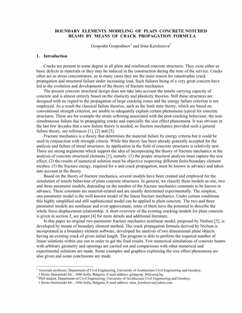
BOUNDARY ELEMENTS MODELING OF PLAIN CONCRETE NOTCHED BEAMS BY MEANS OF CRACK PROPAGATION FORMULA

Gospodin Gospodinov1 and Irina Kerelezova2

1. Introduction

Cracks are present to some degree in all plain and reinforced concrete structures. They exist either as basic defects in materials or they may be induced in the construction during the time of the service. Cracks often act as stress concentrators, so in many cases they are the main reason for catastrophic crack propagation and structural failure under increasing load. Such failures being of a very great concern have led to the evolution and development of the theory of fracture mechanics.

The present concrete structural design does not take into account the tensile carrying capacity of concrete and is almost entirely based on the elasticity and plasticity theories. Still these structures are designed with no regard to the propagation of large cracking zones and the energy failure criterion is not employed. As a result the classical failure theories, such as the limit state theory, which are based on conventional strength criterion, are unable to adequately explain certain phenomena typical for concrete structures. These are for example the strain softening associated with the post-cracking behaviour, the non-simultaneous failure due to propagating cracks and especially the size effect phenomena. It was obvious in the last few decades that a new failure theory is needed, so fracture mechanics provided such a general failure theory, see references [1], [2] and [3].

Fracture mechanics is a theory that determines the material failure by energy criteria but it could be used in conjunction with strength criteria. While this theory has been already generally accepted for the analysis and failure of metal structures, its application in the field of concrete structures is relatively new. There are strong arguments which support the idea of incorporating the theory of fracture mechanics in the analysis of concrete structural elements [1], namely: (1) the proper structural analysis must capture the size effect; (2) the results of numerical solution must be objective respecting different finite/boundary element meshes; (3) the fracture energy, required for a unit crack propagation, must be known in advance and taken into account in the theory.

Based on the theory of fracture mechanics, several models have been created and employed for the simulation of tensile behaviour of plain concrete structures. In general, we classify these models as one, two and three parameter models, depending on the number of the fracture mechanics constants to be known in advance. These constants are material-related and are usually determined experimentally. The simplest, one-parameter model is the well-known model of the linear fracture mechanics. Under certain conditions this highly simplified and still sophisticated model can be applied to plain concrete. The two and three parameter models are nonlinear and even approximate, some of them have the potential to describe the whole force-displacement relationship. A short overview of the existing cracking models for plain concrete is given in section 2, see paper [4] for more details and additional literature.

In this paper an original two-parameter fracture mechanics nonlinear model, proposed by Nielsen [5], is developed by means of boundary element method. The crack propagation formula derived by Nielsen is incorporated in a boundary element software, developed for analysis of two dimensional plane objects having an existing crack of given initial length. The program is able to perform the required number of linear solutions within one run in order to get the final results. Few numerical simulations of concrete beams with arbitrary geometry and openings are carried out and comparisons with other numerical and experimental solutions are made. Some examples and graphics explaining the size effect phenomena are also given and some conclusions are made.

1 Associate professor, Department of Civil Engineering, University of Architecture Civil Engineering and Geodesy, 1 Hristo Smirnenski blv., 1046 Sofia, Bulgaria, E-mail address: gospgosp_frf@uacg.bg 2 PhD student, Department of Civil Engineering, University of Architecture Civil Engineering and Geodesy, 1 Hristo Smirnenski blv., 1046 Sofia, Bulgaria, E-mail address: irina_kerelezova@yahoo.com

2

εf =w/hc

u displacement

w

σE w=hcεf

σE

FF

band with "smeared" crackshc

ε

σ/Eδ functionε deformation

σ/E

line crack

smooth functions u, ε

F

u displacement

deformation

(a)

(b) and (c)

Figure 2 Kinematic description of the fracture process zone: (a) strong discontinuity; (b) weak discontinuity;(c) no discontinuity

(c) "smeared" model(a) real crack in a body (b) discrete model

Figure 1 Discrete and smeared (band) modeling of fracture zone

2. An overview of the existing cracking models for concrete

The mechanical behaviour of quasibrittle materials, such as concrete, rock etc., is mainly characterized by the localization of strain and damage in a relatively narrow zone (fracture process zone), where a macroscopic stress-free crack is gradually developed, see Figure 1 (a). The mathematical modeling of such a zone of highly concentrated microcracks is the key issue in the numerical simulation, therefore it is usually used as a basis of classification of the cracking models.

Discrete and smeared types of modeling of the “fracture process” zone

Two different approaches are available for the proper simulation of the tensile cracking of concrete in the fracture process zone. These are discrete and smeared crack models, see Figure 1 (b) and (c). In its earliest applications , see reference [6], the cracks in concrete were modelled discretely. The discrete crack is usually formed by separation of previously defined finite element edges, if the finite element method is used in the analysis. The nonlinear process is lumped into a line and nonlinear translational springs are usually employed. The symmetric mode I is assumed for simplicity, therefore the crack path is known in advance. The discrete crack approach is very attractive from physical point of view as it reflects the localised nature of the tensile cracking and associated displacement discontinuity. Some drawbacks are however inherent for this approach, namely: the constraint that the crack trajectory must follow the predefined element boundaries and the increasing cost of the computer time because of the additional DOF.

That was the reason for researchers to search for another method and they introduced the smeared crack approach, see references [7] and [8], where the nonlinear strain is smeared over a finite area or band with given thickness. Before going further, it is worth considering the mentioned models from the point of view of the kinematic description of the fracture process zone. Consider a simple homogeneous bar with linear, one-dimensional behaviour, until the fracture process zone develops, Figure 2. Then, following references [1] and [9], we distinguish three types of kinematic descriptions, depending on the regularity of the displacement field u(x). The first one, see Figure 2 (a), incorporates strong discontinuity, i.e. jump in displacement w and strain field ε(x), which consists of a regular part, obtained by differentiation of the displacement function u(x), and a singular part, which can be expressed by Dirac delta function. It is very natural therefore, to relate the kinematic description of Figure 2 (a) to discrete crack approach. At this stage we do not discuss the material model, that is (σ−w) or (σ−ε) constitutive relationship,

3

or mathematical difficulties associated with discrete cracks upon application of kinematic model with strong discontinuity.

The mathematical problem can be regularized by employing another type of kinematic description, given in Figure 2 (b), which corresponds to smeared crack model of Figure 1 (c). That is a continuum model very similar to plasticity models, but when the crack propagation process is continuously developing, the stress-strain relation exhibits softening, instead of hardening. From kinematic point of view, it represents the region of localized deformation by a band of a small but finite thickness hc, separated from the remaining part of the body by two weak discontinuities. The displacement field remains continuous but the strain components experience a jump, so if we assume that the nonlinear (due to cracks) strain is uniformly distributed over the band, we find εf=hcw, where w is easily calculated from the FE/BE solution. We shall leave the question for the choice of band thickness hc open for further discussion.

In its pioneer’s paper [7], Rashid did not employ properly the constitutive (σ - w ) relation, so the numerical solution was mesh dependent. The method was therefore reformulated in paper [8] by including an energy criteria and fracture mechanics principles in it. Fixed and rotational smeared crack versions were developed in [10] and [11], suitable for FE program implementation. Although after 1970’s the smeared crack approach was continuously implemented and used in the general-purpose programs like ANSYS, ABAQUS, DIANA etc., it has not escaped criticism. The principle objection against was that it would tend to spread the crack formation over the entire structure, so it was incapable to predict the real strain localisation and local fracture. As a result a new return to the discrete cracks is noted in recent time using different numerical methods plus interactive-adaptive computer graphics techniques [12[, as an integral part of the analysis process.

Finally, we can explore the most regular description - see Figure 2 (c) with smooth functions u(x) and ε(x), where the displacement field is continuously differentiable and the strain field remains continuous. These are the so-called non-local, gradient or "enhanced strain" models [1], [9], [13] and [14], but we shall not make comments on these methods in the present paper. One-parameter model of Linear Elastic Fracture Mechanics (LEFM)

We begin with the introduction of the simplest model of the linear elastic fracture mechanics called one-parameter model. Consider a specimen made of ideally brittle material (for example glass), having a crack of length a. When a load is applied, the structure can supply a potential energy U at the rate dU/da=G, termed as an energy release rate. On the other hand, the crack propagation at the crack tip needs to consume some energy, which we denote as W at the rate dW/da=R, termed as a fracture resistance. Consequently, the linear elastic fracture mechanics criterion for crack growth is defined as follows:

G=R , (1)

In the LEFM, R is a material constant and is denoted sometimes as Gc , whereas G is a function of the structural geometry and applied loads. The latter can be easily obtained by performing a linear elastic solution using a certain numerical method such as FEM or BEM. The energy-based criterion (1) can be also written in terms of stress intensity factor (SIF) K, using the relation:

G=K2/E’ , (2) where E’=E for plane stress, and E’=E/(1-ν2) for the plane strain, and E and ν are the elastic modulus and the Poisson’s ratio of the material.

As well known SIF K relates the intensity of the crack-tip stresses and deformations to the imposed loading. Therefore, the criterion (1) can be alternatively written as:

K=Kc , (3) where as known from LEFM theory Kc=(E’.R)1/2 is termed as the critical stress intensity factor and is considered to be a material constant, obtained through an experiment.

4

Figure 3 Brittle to ductile transitional behaviour of TPB test made fromquasibrittle material due to change of dimensions

Deflection

Load Brittle behaviour

Ductile-brittle behaviour

Ductile behaviour

It should be also mentioned that according to LEFM principles, the supplied energy during fracture is dissipated only at one point – that is the crack tip. We classify this approach of LEFM as one-parameter model, since the only new material constant related to fracture is R or Kc and the only equation, postulating the beginning of the crack propagation is equation (1) or its equivalent equation (3).

The main problem for the direct application of the LEFM to the concrete structures, having an initial crack, is the fact that the concrete is a typical quasibrittle material. We specify as quasibrittle those materials that exhibit moderate strain hardening prior to the attainment of ultimate tensile strength and tension softening thereafter. It is quite clear today that the principal reason for the deviation of the fracture behavior of concrete and other quasibrittle materials from LEFM is the existence of a fracture process zone ahead of the crack tip, which is not small enough compared to the structure dimensions. That is the consequence of the progressive softening of the material due to microcracking.

The LEFM, even the one-parameter model, could be applied for concrete provided we have to analyse a large–sized concrete element. In the literature that is called structural size-effect phenomenon and is a matter of great amount of scientific publications [1], [2]. The size of the concrete element (in most cases we use the height of the beam D, as a characteristic size) is closely related to its behaviour and the mode of fracture, see Figure 3, where three typical failure modes are shown, depending on the size of the concrete beam.

An assessment is made in reference [15] on the influence of the dimensions of the concrete beam to the type of behaviour and the mode of the structural failure. A special “spring” FE cohesive crack model is employed, and the fracture mechanics data is specially adjusted in the spring’s constants, bearing in mind the size of the FE mesh. A number of numerical solutions are performed on a three-point concrete bend beam, loaded with a concentrated force F at the middle, having an initial crack of length a0=D/2 and it is proven that the model is able to successfully analyse the whole range of beams having different dimensions. It is shown when the methods of LEFM could be applied to concrete and how that relates the beam dimensions and other FM parameters. In [15] the performance of the LEFM model is improved by using the Irwin’s idea of “small but non zero” fracture process zone, taking into account first and second order estimate of the nonlinear zone ahead of crack tip. In general, that is the simplest application of the idea of the effective elastic crack approach involving an iterative procedure in solution and we call it an enhanced Irwin’s approach.

Finally, it is worth to note that the only output result from a LEFM solution, using one-parameter model, is the value of peak (maximum, critical) load Fcr. Two-parameter model of Jenq and Shah

It belongs to the class of effective crack or two-parameter models, and can be classified as to Griffith-Irwin model, see references [1], [2], [3]. Sometimes in the literature they are called equivalent elastic crack methods and they belong to the class of approximate nonlinear fracture mechanics models. The principal idea is that the actual crack is replaced by an effective elastic crack substitute, governed by LEFM criteria. The equivalence between the actual and the corresponding effective crack is prescribed explicitly in the model and it usually involves an element of nonlinear behaviour. Those type of models are able to predict, in principle, peak loads only of pre-cracked specimens of any geometry and size, but they have no potential (unlike cohesive models) to describe the full force-displacement relationship.

Jenq and Shah [16], proposed a two-parameter fracture model shown, in Figure 4. In their approach, the independent material fracture properties are the critical stress intensity factor Ks

Ic and the critical crack tip

5

opening displacement (CTOD)c , which are defined in terms of the effective crack. The fracture criteria for an unstable crack are:

KI=KsIc ,

CTOD=(CTOD)c , (4) where KI is the stress intensity factor, calculated for the given load at the tip of the assumed effective crack of length aeff=a0+∆a, and (CTOD) is the crack tip opening displacement, calculated at the initial crack tip.

In this model, the effective crack exhibits compliance equal to the unloading compliance of the actual

structure, see the Figure 4 (b). It is measured from the test of a three point bending specimen, so the nonlinear effect is included in the solution by experimentally obtained material parameters of the method. The procedure for obtaining experimentally the parameters of the Jenq and Shah method is given in the 1990 RILEM recommendation. As shown in Figure 4, a three-point bend fracture specimen is tested under the crack mouth opening displacement (CMOD). After the peak, within 95% of the peak load Fmax the unloading compliance Cu is measured. Using Cu and the initial compliance C0 along with LEFM equation, the corresponding critical effective crack length aeff can be determined. Consequently, again using the given LEFM relations, Ks

Ic and (CTOD)c of the material can be obtained at the critical load Fmax [1], [3]. This approach is proven to yield size-independent values for the two material constants and for any other geometry as well, [3].

Another well-known two-parameter model is proposed by Karihaloo [2]. However, the effective crack length aeff is calculated not from the unloading compliance, but from secant stiffness of the real concrete specimen at a peak load. The suggested fracture criteria are very similar to equations (4) and the procedure for obtaining the two material parameters is explained in details in reference [2].

The class of effective crack, two-parameter models (such as: the size effect model; the R curve concept; elastic equivalence methods etc) take advantage of the well-documented pre-peak nonlinear behaviour of concrete. They are able to give a good estimate of the critical (peak) load, but in order to obtain a complete description of the response past the peak load, using these models, additional assumptions have to be invoked. The answer is either development of the class of three-parameter models or the enhanced, two-parameter model of Nielsen, which will be given a special attention in this paper.

Fmax

F

Cu

C0

1

1

KI=K sIc

CTOP=(CTOD )c

ac

a0 ∆ac

a0

∆ac

ac

F

notch

CTOP

CTOPelCTOPcr

unloadingat peak load

Figure 4 Jenq and Shah two-parameter model: (a) Fracture criteria: KI=KsIc and

CTOP= (CTOD )c ; (b) Determination of KsIc and (CTOD) c from C0 and Cu

(a) C0 and Cu are the initial compliance and theunloading compliance at the peak load

(b)

6

Three-parameter models of fracture mechanics (cohesive type models) The first three-parameter nonlinear theory of fracture mechanics of concrete was proposed by

Hilleborg et al., [17], and it was named fictitious crack method. It originated from the idea of the cohesive approach due to Dugdale-Barenblatt. Distributed cohesive forces, along the crack faces, which tend to close the crack, simulate the toughening effect of the fracture process zone (FPZ). Therefore, there is no singularity at the crack tip unlike in LEFM and stresses there have finite values.

Hilleborg assumes that the stress-strain constitutive relation is not a unique material property due to the

localization of the deformation in the FPZ. Instead, two separate constitutive relations, inside and outside the fracture zone, are needed for describing the material response, see Figure 5 (a) for the two dissipation mechanisms proposed. The thickness of the fracture zone (the fictitious crack) is zero and the constitutive relation representing the FPZ must include, in addition to continuous displacements, the displacements due to cracking. It is important also to point out that the distribution of the closing stresses σ(w), is a function which depends on the opening of the crack faces, w. The area GF under the curve in the Figure 5 (a) is termed fracture energy and that is the energy consumed in increasing the width of the crack from zero to wc. The fracture energy GF is considered to be a material property and its value can be calculated from the following integral:

)(,)( 5dwwfGcw

0F ∫=

where wc is the critical crack separation corresponding to σ(w)=0. We consider the cohesive approach of Hilleborg as a three-parameter model. Two of them are defined

as material constants, say tensile strength ft and critical separation wc, so the third parameter is usually geometrical, e.g. the type of f(w) function. In the numerical simulation we choose either linear or bilinear form of f(w) function, therefore in this case the fracture energy GF is "adjusted" to the model being calculated from equation (5). Any other combination of parameters GF, ft and wc is possible, provided the form of f(w) function is known (or accepted) in advance.

The idea of Hilleborg was first used in the context of the discrete crack approach having the kinematic description of Figure 2 (a). As a result the mesh dependency, as one of the drawbacks of the analysis of concrete structures, was removed. A similar approach, proposed by Bažant and Oh [18], is the crack band model, see Figure 5 (b). In this model, a crack band zone of thickness hc is introduced to represent the FPZ. In contrast to Hilleborg's approach, the crack band is treated as a continuum described by a stress-strain relation reflecting both: the localized deformation and the continuous deformation. Naturally Bažant's approach turns out to have a kinematic description, shown in Figure 2 (b). It is also considered to be a three-

F F FF

ft

w

σ

ε

σft

areaGF

wc

σ(w)= f(w)

εε

σ

areaGF/hc

wc/hc

ε(w)ft

σ

(a) cohesive method of Hilleborg (a) "band" method of Bažant

Figure 5 Relationship between constitutive curves of cohesive and smeared (band) methods

crackline

band of thickness hcft

7

n-1

FnF2

F1

Ω1

Y

X

Γ

n 321

bΩ2

interface line

two crack facesΓ1

X

FnF2

F1

Y

Γb Ω

aΓ1

opening

(a) (b)

Figure 6 (a) Plane body with initial crack subjected to arbitrary loading; (b) Thestructure discretized with boundary elements divided into two sub-regions Ω1and Ω2

parameter model, where the third parameter is of geometrical type and that is the band width hc. It is proven in references [10] and [11], that the two models, given in Figure 5, are equivalent under certain conditions and this relationship is also shown in the figure. In the same references another variant of the "band" model is developed (fixed and rotational smeared crack models), which seems to be more convenient for a finite element implementation. 3. The BEM applied to crack problems using multi-domain formulation approach

The boundary element method (BEM) is already well established and powerful numerical technique, which is a good alternative of the finite element method. Its main advantages are the higher accuracy of the solution and the fact that the discretization is only on the boundary of the investigated body. Therefore, the number of the unknowns is very small when compared with FEM, which makes the method very efficient. The application of the boundary element method in fracture mechanics and crack propagation analysis has been given a growing attention recently, see references [15] and [19], but when compare with FEM fracture mechanics applications, it is still in a premature state.

In this paper we develop a multi-domain variant of BEM, which means that the crack path is known in advance. Decomposition is made of the plane body into sub-regions with a line boundary between, containing the crack to be eventually developed. A short description of the theory follows.

Consider a two dimensional domain Ω with an opening under plane stress or plane strain condition. It is subjected to distributed load b in the domain and concentrated forces F1, F2,.. Fn on its boundary Γ , see Figure 6 (a). The plane body has an arbitrary shape of the contour and contains an initial crack of length a plus an opening with contour Γ1. There are some supporting links on the boundary or it could be continuously supported. Part of the boundary can be subjected to external tractions. It is well known that starting from Betti's reciprocal theorem the integral equation of the problem may be derived, from where the boundary integral equation may be formulated, [20]. Without going into details, using tensor notation for simplicity and disregarding the effect of the concentrated forces for clarity of the equation, we write the following boundary integral equation:

( ) ( ) ( ) ( ) ( ) ( ) ( ) ( ) ( ) ( ) ( )∫∫∫ΩΓΓ

Ω+Γ=Γ+ xdxbxuxdxpxuxdxuxpuc jijjijjijjij ,,, *** ξξξξξ , (6)

where i, j =1,2 ; ξ and x are the observation and source points, respectively; uj(ξ) is the displacement at ξ; Γ represents the boundary of the body and includes the boundary of the opening Γ1; Ω represents the domain of the body; bj(x) is the intensity of the body forces at x; uj (x) is the displacement at x; pj (x) is the traction at x; and the function

−Γ∈

Ω∈=

.,

,,)(

nodesboundartysmoothfor21c

ij

ij

ij ξδ

ξδξ (7)

The well-known Kelvin fundamental solutions ),(),( ** xpandxu ijij ξξ are given by:

8

typical corner pointwith incompatibleelements

Figure7 Three types of linear boundary elements- compatible, right and left incompatible

x

the real boundary 2

1 ξ=1

ξ

ξ= -1

compatible linear boundary element

y

incompatible right linear boundary element

incompatible left linear boundary element

a

[ ] ,))(()()(

,ln)()(

,,,,*

,,*

−−−+−

−−

=

+

−

−=

ijjijiijij

jiijij

nrnr21nrrr221

r141p

rrr143

G181u

ν∂∂δν

νπ

δννπ

(8)

where ν is the Poisson's ratio; G is the shear modulus; r is the distance between the point ξ and the point x; nj is the direction cosines of the outward normal to the boundary; δij is the Kronecker delta symbol.

In order to solve numerically the integral equation (6), we make discretization on the boundary (including Γ1) dividing it to n linear segment and introducing four boundary discrete values - two displacements and two tractions at each boundary node, see Figure 6 (b). Two of these are known and two unknown, so they should be obtained from the numerical solution. If a loading in the domain Ω b is given, a discretization in the domain is also needed using two dimensional elements but with no new unknowns introduced. Note, that in order to consider properly the stresses around the crack tip we divide the body Ω into two sub-regions Ω1 and Ω2. We choose appropriate shape functions for representing the boundary displacements and tractions. In order to obtain convergence in the solution the minimum order of approximation is linear for this type of problems [20], so linear boundary shape functions are used for representing the displacement and traction functions within the linear type boundary elements, see Figure 7.

In local coordinate ξ (-1 to 1 variation within the element) we make the following approximation for the vectors of boundary displacement and traction functions ue, pe:

ue(ξ)=Ne(ξ)ue, pe(ξ)=Ne(ξ)pe, (9) where ue=(ux uy)T is the vector of displacement functions for the element, pe=(px py)T is the vector of traction functions for the element, ue=(u1x u1y u2x u2y)T is the vector of discrete values of displacements of local points 1 and 2 for the element, pe=(p1x p1y p2x p2y)T is the vector of discrete values of tractions of local points 1 and 2 for the element, Ne(ξ) is matrix of shape functions for compatible element, which has the form:

( ) ( )( ) ( ) .)(

+−

+−=

ξξξξ

ξ1010

010121N e (10)

Dealing with corner points of the plane body is one of the most laborious problem to be resolved in

BEM. In the present work we use the idea, developed in reference [20], where so called "incompatible" left and right linear boundary elements are introduced, see figure 7. The corner point is not treated directly, but the nodal point of the element is moved to a small distance a (in our case we take a= 1/3), therefore it is not necessary to satisfy the integral equation at the corner point, because sometimes the boundary conditions are different at both sides of the corner. The matrix of shape functions Ne(ξ) for a left incompatible element is:

( ) ( )( ) ( ) ,)(

+−

+−=

230130023013

51N e

ξξξξ

ξ (11)

9

and for the right incompatible element we have:

( ) ( )( ) ( ) .)(

+−

+−=

ξξξξ

ξ130320

01303251N e (12)

It is well known that the calculation of the stress intensity factors (SIF) of the LEFM requires very

accurate results for the displacement and stress fields around the crack tip. On the other hand the stresses at the crack tip are singular, which makes the task very complex. We use the so-called "singular" displacement boundary elements, derived for first time in reference [15], which put at the crack tip, will lead to considerable improvement of the numerical results for a relatively coarse mesh. The corresponding displacement shape functions are of such a type, that the first derivative with respect to local coordinate ξ has singularity of order O(r−1/2), which is in accordance with the required stress singularity.

In order to get the discretized analog of the boundary integral equation (6) we put equation (9) into (6) and do the integration. Usually a numerical integration is performed (in this case we use 10 points Gaussion quadratures) and this leads to the following system of matrix equation:

HU+B=GP, (13) where U is the vector of all nodal boundary displacements, P is the vector of all nodal boundary tractions, B is calculated vector, representing the effect of the external loads, H and G matrices are calculated using the numerical evaluation of the boundary integrals, which contain the fundamental solutions and shape functions.

After the boundary conditions are satisfied in equations (13), we obtain and solve the final system of linear algebraic equation and get the numerical set of boundary displacements and tractions. Once we have the boundary data available, we go further and obtain the displacements and stresses at a given point from the domain Ω , using again equation (6) for displacements and the following integral equation for stresses:

( ) ( ) ( ) ( ) ( ) ( ) ( ) ( ) ( ) ( )∫∫∫

ΩΓΓ

Ω+Γ−Γ= xdxbxuxdxuxpxdxpxu kijkkijkkijkij ,,, *** ξξξξσ , (14)

where the tensors uijk* and pijk

* can be found elsewhere [19]. In order to check the LEFM criterion for crack propagation, we have to calculate the SIF or the energy

release rate, if necessary. In the next section the numerical procedures adopted will be explained. 4. Crack propagation formula and its incorporation in the boundary element code

In the theoretical paper [5], Nielsen proposes a simplified fracture mechanics model for crack growth

of quasibrittle materials, based on an energy balance equation. The newly developed formula was evaluated by Olsen [21], for studying the crack propagation in three point bending concrete beams. The numerical procedure requires determination in advance of the change of the elastic strain energy with crack length a (i.e. dW/da function), which can be done by a simple FEM calculation. We begin with short presentation of the main points of the theory and the assumptions made.

Consider a plane body with an internal crack of length a, subjected to load, applied at the boundary. At the critical moment, when the crack is on the verge of extension, the following energy balance equation is valid, as stipulated by Griffith, [21]:

dW/da+GFb=0, (15) where W the strain energy stored in the body of width b, GF is the fracture energy and for the sake of simplicity only the case of displacement controlled systems will be examined in this paper.

As stated above, the first term of equation (15) is called driving force, whereas the fracture energy GF can be viewed as a crack resisting, material parameter. Using Irwin's idea for introducing a small, but

10

w0/2

leff

w0/2

a'pa

ap

x

ft

proposed stress distributionof cohesive forces

σ

elastic

x

the tip of the effective crack

the real stress distribution

Figure 8 The stress field for concrete around crack tip and ope-ning displacements with and without cohesive stresses

finite nonlinear zone in the crack tip [1], and making some approximate energy consideration, Nielsen suggests the following equations, [5]:

2t

2I

p fK1a

π=′ , (16)

2t

2I

peff fK40a40l

π.. =′= . (17)

where ap' is the length of the fracture process zone of the model, leff is the effective crack length term, KI is the stress intensity factor and ft is tensile strength the concrete, see figure 8.

The length of the fracture zone ap' is obtained by the well known Irwin's equilibrium conditions, see [5] and [21], under the following two simplifying assumtions: (1) the type of (σ−w) relation for the softening curve is not taken into account; (2) in considering an elastic-brittle material, the real distribution of the cohesive stresses is presented as rectangular along a part ap' of the actual fracture zone ap. Therefore, as seen from equation (16), we get an Irwin type approximation for ap'. As for is the effective crack length term leff , an assumption is made to take into account the work of cohesive stresses by using a simplified crack opening displacements formula, according to LEFM (see reference [5], equation (3.8)).

Now, having the effective crack length term leff , obtained by this extremely simplified analysis, Nielsen suggests to consider the energy available on the basis of an effective crack length aeff=a+ leff , instead of the real crack length a. Bearing in mind that for the possible crack growth the increment ∆leff is a positive function of both crack length and displacement u, starting from equation (15) and after some alterations, we get the following final equation:

∂

∂+

∂∂

−

∂

∂

∂∂

−=

al

1aWbG2

ul

aW

duda

effF

eff

. (18)

Equation (18) is the Energy Balance Crack Propagation formula for a displacement controlled system.

In fact, that is a first order differential equation with respect to the crack length function a, where the derivative ∂W/∂a is taken at a+ leff, while ∂leff/∂a may be taken at a. It is impossible to solve the differential equation (18) analytically, so as in reference [21], we explore the fourth order Runge Kutta method. It is very important to note, that the crack propagation formula takes into account the plastic behaviour near the crack tip by putting (17) in it, although it is based on the calculation of elastic energy W (u,a) and its derivative ∂W/∂a. The latter term is used for the calculation of the stress intensity factor in (17) by exploring the well known LEFM relation, see also equation (2). The accuracy of the adopted numerical procedure for the solution of (18) depends on the number of "loading" steps, which is actually the number of divisions of

11

the imposed displacement u from its initial value u0 to its final one umax. After the current solution step is performed, having the increment of the real crack length ∆a, we calculate the effective crack length aeff as:

aeff=a+leff+∆a, (19) where a includes the initial crack length plus sum of increments ∆a, as calculated in the previous steps.

Within every step, using the current value of displacement u , the calculated value of W and updated

aeff, we calculate the force response F from the relation W=Fu/2. It is presumed in this paper, that only one boundary link is moving and the crack path is known in advance (symmetric fracture mode I). In such a way we are able to obtain the force-displacement curve for the whole (u0 - umax) interval.

The described numerical procedure is implemented into a boundary element program called BEPLANE. To be more readable, the relevant flow chart given in Figure 9, is supplied with some equations.

START: u = uo; a =aoLinear Solution (LS) – KI =..

effeff laa +=

u = u; a =aeff determination of F = F(u,aeff)

Runge Kutta method

∂

∂+

∂∂

+

∂

∂

∂∂

−=

al

1aW

bG

ul

aW

duda

effF

eff

aaanew ∆+=

maxuu >

STOPYes

BEPLANE LS – KI=..u = u + du; a = anew

32 LS for 1 loading step

j = 1,4 calculation of kj

( )4321 kk2k2k61a +++=∆

2t

2I

eff fK40l

π,=

No

Figure 9 The flow chartfor theimplementednumericalprocedure

12

To perform a full, fourth order Runge Kutta procedure within one displacement step, 32 linear elastic solutions are needed for different values of arguments a and u. Full details of methods and procedures for calculation of derivatives within BEPLANE can be found in reference [15].

As a first illustration of the potential of the theoretical model and the boundary element program, we

do a numerical simulation on a three point bending concrete beam. The input data is taken from reference [21] and is given in the Table 1. A vertical displacement at the middle of the beam (0 ÷ 2 mm) is imposed to Table 1

E = 42210 N/mm2; ν = 0,2; GF = 0,0957 N/mm; ft = 6,86 N/mm2; L=8D; D = 100 mm; ao = 50 mm

Point u [mm] F [N] a + ∆a [mm] leff = 0,4 pa′ [mm] pa′ [mm] aeff=a + ∆a + pa′ [mm]

A 0.08 1066.85 50.146 1.746 4.3646 54.510

B 0.15 1572.95 52.280 6.0816 15.203 67.482

C 0.19 1349.97 57.285 9.3906 23.476 80.761 simulate the behaviour of the displacement controlled system. The main purpose of this numerical test is to show and estimate the continuous change of few important geometrical parameters for the three "state"

points A, B and C. That is why only the middle part of the beam is shown in Figure 10 (a) and the parameters plotted in a real scale are as follows: areal=acur+∆a, (fourth column); leff = 0,4a'p (fifth column); a'p (sixth column) and aeff=a + ∆a + a'p , (last column). The force-displacement relationship is presented in Figure 10 (b) and the state points A, B and C are shown in order to make some conclusions. Point A indicates the end of elastic behaviour and the beginning of the pre-critical process zone development. The length of the real crack is 50.146 mm and the effective crack length - 54.51 mm. The length of the fracture zone is just 4.3646 mm which takes about 9 % of the ligament. The critical state, corresponding to Fmax, is

C

B

A

0200400600800

10001200140016001800

0 0.05 0.1 0.15 0.2

Displacement [mm]

Force [N]

Figure 10 (a) Real scale graphical presentation for areal, leff and a'p for state points A, B and C of the three point bend speciment; (b) Force-displacement diagram illustrating points A, B and C

(b)

A B C

leffpa′

a + da

leff

a + da

Dleff

a + da

pa′

pa′

13

Geometry and material dataE = 42210 N/mm2

ν = 0.2D = 100 mmb = 100 mmGF = 0.0957 N/mmft = 6,86 N/mm2

D

Figure 11 A three-point bend specimen loaded symmetrically

F

0,5D

b

L=8D

reached at point B. The a'p zone is spread over 1/3 of the ligament (15.203 of 50 mm) and the crack extension as already 2.28 mm. C is considered as the failure point for the theoretical model. If we continue the numerical process applying the next increment of displacement, the results received are meaningless, because the length of effective crack will "jump" over the ligament. We conclude therefore, that the theoretical model and the proposed numerical solution have the potential to describe the entire pre-critical nonlinear zone and part of the post-critical branch (strain softening zone). The critical force Fmax can be obtained within the solution as well. How far are these quantities from the reality will be a matter of discussion in section 5.

It is now time to pose the important question: where can one place the model, proposed by Nielsen in reference [5], in the context of the review made in section 2. In our view that is an enhanced two-parameter model. The motivation is as follows: (1) the fracture mechanics parameters employed are two, namely: tensile strength ft and the fracture energy GF; (2) The form of σ(w) relation in the softening branch is ignored for the sake of simplicity, therefore the usual geometric parameter in the three-parameter models is missing. Why enhanced? Because: (1) "in a way" the contribution of cohesive forces is taken into account; (2) the model has the potential to completely describe the pre-peak force-displacement nonlinear relationship, and partly the post-peak force-displacement relationship. 5. Numerical results and comparisons

Comparison with experimental results and other numerical solutions

The aim of this numerical test is make a comparison of the load-deflection curve we get from the present numerical solution with the experimental test and other available numerical results. Consider the concrete beam shown in Figure 11. The geometry and material data are taken from reference [21], where an experimental test on this beam (named A-B100.3) has been performed. The boundary element model takes only half of the beam due to symmetry. Two sub-domains are discretized in order to get better results and a singular incompatible boundary element is placed at the tip of the crack. The BE mesh consists of 90 boundary elements (about 200 DOF), this number is changing dynamically during the process of crack propagation. A refined BE mesh around the crack tip and corner points is envisaged. A vertical displacement at the point in the middle of the beam is performed incrementally and the relevant reaction force F is calculated.

The load-deflection curve from the numerical solution is shown in Figure 12. The same relation, taken from the experiment, is also enclosed for comparison. Another, cohesive type numerical solution for the same concrete beam is also given for completeness. A discrete crack approach is employed using two-dimensional finite elements for representing the concrete plus nonlinear translational springs for simulation of the crack development. To complete the model a simple procedure was implemented in the general purpose software system ANSYS, see reference [15] for details.

On examination of the three graphics from Figure 12, it could be concluded that the two numerical solutions are giving quite reasonable results as far as the peak force Fmax is concerned. The pre-critical nonlinear part of the curves are also very close, although the displacements are bigger compared with the experiment. In the post-critical zone a different picture is observed. The FEM cohesive solution behaves well covering the whole softening branch of the F-u relation. The present BEM crack growth formula solution stops at value of displacement u=0.20 mm, as expected from the theory. Therefore, the proposed

14

fracture mechanics theoretical model has the potential to simulate the behaviour of concrete beam within the framework of the limitations, already mentioned.

Analysis of a concrete beam with complex geometry and openings

The objective of the next numerical test is to demonstrate the versatility of the BE approach. The program is able to solve plane objects having arbitrary contour geometry including openings. By using the multi-domain techniques approach, different material properties can be considered. A symmetrical concrete beam with four openings is drawn in Figure 13. Geometrical and material data are also enclosed.

Due to symmetry half of the beam is considered. In addition, the beam is divided into two sub-domains. The boundary element mesh, which includes the contours of the openings, the boundary conditions symbols and the deformed shape (for a certain solution step) are shown in Figure 14, in the manner they are displayed in the postprocessor of BEPLANE. Again a vertical displacement of the middle point is performed.

Beam and Fracture data:E = 30000 N/mm2; ν = 0,2; ft = 3,3 N/mm2; GF = 0,1 N/mm; b=50 mm

400400 mm

75

125

25

25

50

25

25

50 150 50 75 200 100 100

75

Figure 13 A three-point beam loaded symmetrically having an initial crack of length a0 =0,25D

A - B100.3

0

250

500

750

1000

1250

1500

1750

0 0.15 0.3 0.45 0.6 0.75

Force

BEM - Crack Growth formula FEM - cohesion solution Experiment

Figure 12 Comparison of results for load-deflection curves for beam A-B100.3

Displacement

15

Other graphics, taken from the BEPLANE postprocessor are given in Figure 15. We call it "monitor

process" window, and it is specially designed for the program user to follow the computational process on-line. It consists of four windows, as follows:

Figure 14 The BE mesh and the deformed shape of the beam as displayed in BEPLANE

Figure 15 The BEPLANE on-line "monitor process" window

16

(1) BEPLANE logo and some input data; (2) On-line appearing plot of the force-displacement curve. From this curve the consumed fracture

energy is calculated as follows, [21]: Gcalc=∆A /b/∆a , (20)

where ∆A is the external energy supplied, which can be calculated from the area under force-displacement curve, b is the thickness of the body and ∆a is the length of the fully developed part of the crack;

(3) G-verification window where on-line calculated values of fracture parameter GcalcF are plotted against the input parameter GF. During the computational process the two current values are displayed on the right side of the monitor;

(4) A graphic of the real crack growth a against the corresponding displacement value u. As seen from the particular graphic, in the displacement range between (0 ÷ 1 mm) no substantial crack growth is observed. As the load approaches its critical (peak) value, the gradient of the crack growth function has gradually increased. Additional useful data appears on the right side of the monitor to help the user, such as the current stress intensity factor KI and others.

The force-displacement relation graphic for the beam into consideration is shown in Figure 16. Another solution for the same beam is made using ANSYS cohesive model and the relevant curve is also plotted in the figure with thinner line. It can be seen (assuming the cohesive solution is reliable enough) that the crack propagation formula applied in conjunction with boundary elements is able to predict the peak load (the difference is within 4 %) and the ascending branch of the curve. As in the case of the previous example, the theory is only able to predict a part of the descending branch of the load deflection curve.

It should be mentioned however, that the particular beam geometry was especially chosen as a purely "academic" test. In reality, the onset of crack propagation in such a concrete beam is likely to develop at the corner points of the openings in line with the development of the major crack. The present approach considers the development of one crack only.

E = 30000; G f = 0.1; ft = 3.3; ν

= 0.2; b = 50 mm

1014.987

1061.27

0

200

400

600

800

1000

1200

0 0.05 0.1 0.15 0.2 0.25 0.3

Displacement

Force

BEPLANEANSYS

Figure 16 Force-displacement curves from present method and ANSYS cohesive approach

17

Size effect prediction numerical test Since the presented theory determines the load carrying capacity (Fmax) of the concrete structures upon

the conditions and limitations described, it should be able to predict the size effect, i.e. it should be able to give the load carrying capacity as a function of absolute values of a chosen geometrical parameter (that could be D dimension in our case), characterizing the size of the structure. As in reference [21], it is convenient to use a common value B, as a measure of brittleness of the structure:

EGDf

BF

2t= , (21)

where the parameters in the right side of equation (21) are already defined. Table 2

The size effect is rigorously defined through comparison of geometrically similar structures of different

D sizes, provided all other dimensions keep the proportions. The same effect might be achieved by using the B parameter (or any component of B) instead of D. We consider again the concrete beam from Figure 13 and keeping the standard values of the parameters D, ft and modulus E, we vary Gf from 10000 to 0.01.

10000 3.30 30000 25 100 3.63E-06 1197.260318 1.547973 plastic100 3.30 30000 25 100 0.000363 1196.946628 1.547567 plastic10 3.30 30000 25 100 0.00363 1194.613960 1.544551 plastic1 3.30 30000 25 100 0.0363 1171.497187 1.514663 quasibrittle

0.5 3.30 30000 25 100 0.0726 1148.687751 1.485172 quasibrittle0.2 3.30 30000 25 100 0.1815 1089.848953 1.409098 quasibrittle0.1 3.30 30000 25 100 0.363 1014.986815 1.312306 quasibrittle

0.05 3.30 30000 25 100 0.726 913.432510 1.181004 quasibrittle0.02 3.30 30000 25 100 1.815 735.105509 0.950439 brittle0.01 3.30 30000 25 100 3.63 599.736424 0.775417 brittle

GF ft E ao Fmax σ/ftD B Type of behaviour

-0.12

-0.08

-0.04

0

0.04

0.08

0.12

0.16

0.2

-5.6 -4.8 -4 -3.2 -2.4 -1.6 -0.8 0

Log (B)

Log

(/f t

)

LEFM

plastic

quasibrittle

Figure 17 Structural size effect represented by failure load versus brittelness number B

18

A set of ten numerical solutions is performed with the present theory for different values of Gf and the load carrying capacity Fmax is obtained, see Table 2. The results are also depicted in Figure 17, where brittleness number B versus (σ/ft) in a logarithmic scale is shown. Note that following [21], Fmax has been given a dimensionless form as a Navier stress along the depth (D-a0).

Before making comments on the results from Table 2 and Figure 17, it is instructive to plot and

examine the force-displacement graphics for the same concrete beam. That is done in the Figure 18 from where the different modes of failure are clearly indicated.

Let us first consider the two solutions corresponding to smallest values of fracture energy, GF=0.01and GF=0.02, see the last two rows of the Table 2, the respective points from Figure 17 and relevant curves from Figure 18. The failure modes are typical for a perfectly brittle structure and it can be easily proven that the values of Fmax can be simply related to the SIF, calculated by using principles of the LEFM, [21]. Note also, that the two points from the Figure 17 are placed on the inclined straight line of slope -1/2, which is a well-known fact from the size effect theory of LEFM, [1]. Therefore, concrete structures having parameters within the same range, can be classified as brittle, i.e. they experience a brittle type of behaviour. Absolutely the same situation will apply for concrete structures with big D dimension, but having the same B parameter. The simplified methods of LEFM can be applied in such a case and the size effect law is valid. The presented theory is able to easily cover this type of behaviour.

On the other hand it could be noted from Table 2 that for the first three solutions the Fmax values are almost equal and the respective failure modes are typical for plastic type of behaviour. That corresponds to big values of fracture energy (GF=10,100, 10000 ) or smaller absolute values of characteristic dimension D. No size effect is observed in this case, so any nonlinear classical failure theory, which uses some type of strength limit or failure surface in terms of strain or stress, may be applied. Therefore, the nominal strength for these type of structures is independent from the structural size and we classify them as plastic structures.

E = 30000; ft = 3.3; ν = 0.2; b =50

0

200

400

600

800

1000

1200

1400

0 0.05 0.1 0.15 0.2 0.25 0.3

Displacement

Force

GF = 10000GF = 100GF = 10GF = 1GF = 0.5GF = 0.2GF = 0.1GF = 0.05GF = 0.02GF = 0.01

Figure 18 Force-displacement curves for the beam of figure 13 varying the fracture energy GF

brittle

plastic

quasibrittle

19

It is clear from the above discussion that for concrete structures with small absolute dimensions (plastic type of behaviour) plasticity methods can be applied, whereas for concrete structures with big dimensions (brittle type of behaviour) the LEFM methods are more appropriate. Therefore, between those two extremes when a concrete structures of a medium size is to be analyzed, a transitional behaviour should be expected. That is illustrated as a solid curve in Figure 17. We classify this type of behaviour as quasibrittle. The nonlinear methods of fracture mechanics are applied in this case and they give best results. For values of GF between 0.05 ÷ 1, the present solutions clearly show this tendency. There is no size effect observed but the nominal strength varies with the change of parameter B through changes of GF or D .

The conclusion, made from the results of this numerical test, is that the present theoretical model is able to perform analysis of concrete structures for the whole range of fracture mechanics parameters and structural sizes. 6. Concluding remarks

In this paper the simplified fracture mechanics theoretical model of Nielsen is implemented in the boundary element program BEPLANE. The numerical procedure is integrated in the software program in such a way that the final solution is obtained in one run and there is no need for calculations in advance. The model has shown to be promising for mode I fracture analysis of unreinforced concrete. For a variety of example problems reasonable agreement with the experimental data has been found, not only for the peak load but also in the pre-peak nonlinear zone. The numerical approach allows considering plane concrete structures with arbitrary contour geometry and openings. It was demonstrated that by means of the present approach any type of structural behaviour might be considered starting from ideally brittle through quasibrittle and plastic. A general deficiency of the approach is that only a part of the post-peak softening branch is covered by the solution. Also at present, the method does not include treatment of more then one discrete crack, which can be a topic of future work.

REFERENCES [1] Bažant, Z., J. Planas, “Fracture and Size Effect in Concrete and Other QuasibrittleMaterials”, CRC Press, LLC, (1998). [2] Karihaloo B. L., “Fracture mechanics & structural concrete”, Longman Scientific & Technical, (1995). [3] Shah, S., Swartz, S., and Ouyang., C., “Fracture Mechanics of Concrete: Applications of Fracture Mechanics to concrete, Rock, and Other Quasibrittle Materials” , John Wiley & Sons, Inc, (1995). [4] Gospodinov, Gospodin, "Review of the Computational Models for Cracking of Quasibrittle Materials",(in Bulgarian), Annuaire de l’Universite d’Architecture, de Genie Civil et de Geodesie, Sofia, Jubilee Session, (2002). [5] Nielsen, M. P.: An Energy Balance Crack Growth Formula, Bygningsstatiske Meddelelserm Edited by Danish Society for Structural Science and Engineering, Volume 61, No 3-4, pp. 1-125, (1990). [6] Ngo, D., and Scordelis, A. C., “Finite Element Analysis of Reinforced Concrete Beams”, Journal of the American Concrete Institute, Vol. 64, No 3, pp.152-163, March (1967). [7] Rashid, Y. R., “Analysis if Prestressed Concrete Pressure Vessels, Nuclear Engineering and Design, Vol. 5, No 4, pp. 334-344, (1968). [8] Bažant, Z. P., and Cedolin, L., “Blunt Crack Band Propagation in Finite Element Analysis”, Journal of the Eng. Mechanics Division. ASSCE, Vol. 105, No EM2, pp. 297-315, (1979). [9] M. Jirásek and B. Patzák, Models for quasibrittle failure: Theoretical and computational aspects, Second European Conference on Computational Mechanics,(ECCM), Cracow, Poland, June (2001). [10] Rots, J. G. and Blaauwendraad, J., Crack modeling for concrete: Discrete or smeared? Fixed, multi-directional or rotating? HERON, vol. 34, No 1, Delft UT, (1989). [11] Rots, J. G. et al., Smeared crack approach and fracture localization in concrete, HERON, vol. 30, No 1, Delft UT, (1985).

20

[12] Ingraffea, A. R., and Saouma, V., Numerical modeling of discrete crack propagation in reinforced and plain concrete, in Fracture Mechanics of Concrete, EAFM, eds. G. Sih and A. diTommaso, (1985). [13] de Borst, R., and Muhlhaus, H., Continuum models for discontinuous media, in: Fracture Processes in Concrete, Rock and Ceramics, van Mier, J. and al. eds., RILEM, E&FN Spon, 1991. [14] Akesson, Magnus, Implementation and Application of Fracture Mechanics Models for Concrete Structures, PhD thesis, Chalmers UT, Goteborg, Sweden, (1996). [15] Kerelezova, Irina, Numerical Modeling of Quasibrittle Materials by Means of Fracture Mechanics Approach, PhD thesis, University of Arch., Civil Eng. & Geodesy, Depart. of Civil Eng., Sofia, (2002). [16] Jenq, Y., and Shah, S., A Two Parameter Fracture Model for Concrete, J. Eng. Mech., Vol. 111, No 4, pp 1227-41, (1985). [17] Hilleborg, A., Modeer, M. and Petersson, P. E. Analysis of crack formation and crack growth by means of fracture mechanics and finite elements. Magazine of Concrete Research, Vol. 6, (1976). [18] Bažant, Z. P., and Oh B., Crack band theory for fracture of concrete, RILEM Mat. Struct., 16(93); 155-177, (1983). [19] Aliabadi, M. and D. Rooke, Numerical Fracture Mechanics. Kluwer Academic Publishers, (1991). [20] Gospodinov, G., and P. Drakaliev, On the application of the boundary element method in the plane problems of the theory of elasticity, Journal of theoretical and applied mechanics, Sofia, vol. 2, (1990). [21] Olsen, D. H., Concrete fracture and cracks growth- a fracture mechanics approach, PhD thesis, Department of Structural Engineering, DTU, Series R, No 42, (1998). Acknowledgment: The authors would like to express their gratitude to Professor M. P. Nielsen and Dr. T. C. Hansen for their support and useful discussions during the course of this work.