Bootstrapping high-frequency jump tests:

Supplementary Appendix∗

Prosper DovononConcordia University

Sılvia GoncalvesMcGill University

Ulrich HounyoUniversity at Albany, SUNY and CREATES

Nour MeddahiToulouse School of Economics

November 15, 2017

This supplementary appendix is organized as follows. In Section S1, we first provide an auxiliarylemma and then provide proofs of the general bootstrap results appearing in Section 3 of the mainpaper. In Section S2, we establish the results appearing in Section 4 of the main paper. In particular,this section contains the asymptotic expansion of the cumulants of the asymptotic test statistic Tnand its bootstrap versions T ∗n and T ∗n . The limits of these cumulants are derived by relying on someauxiliary lemmas that are introduced and proved in this section of the appendix. Detailed formulasuseful for the implementation of the log version of our tests are provided in Appendix S3. Finally,Section S4 presents the theoretical justification for the local Gaussian bootstrap when applied to twoalternative jump tests: the test of Podolskij and Ziggel (2010) and the big jumps test of Lee andHannig (2010).

Appendix S1: Proofs of results in Section 3

We first derive the first and second order bootstrap moments of (RV ∗n , BV∗n )′ . Note that since r∗i =√

vni · ηi, we can write

RV ∗n =n∑i=1

vni · ui and BV ∗n =1

k21

n∑i=2

(vni−1

)1/2(vni )1/2 · wi

where ui ≡ η2i and wi ≡ |ηi−1| |ηi|, with ηi ∼ i.i.d. N (0, 1). The bootstrap moments of (RV ∗n , BV

∗n )′

depend on the moments and dependence properties of (ui, wi) . The proof is trivial and is omitted forbrevity.

Lemma S1.1 If r∗i =√vni · ηi, i = 1, . . . , n, where ηi ∼ i.i.d. N (0, 1), then

(a1) E∗ (RV ∗n ) =n∑i=1

vni .

∗We are grateful for comments from participants at the SoFie Annual Conference in Toronto, June 2014, and at theIAAE 2014 Annual Conference, Queen Mary, University of London, June 2014. We are also grateful to two anonymousreferees and an associate editor for many valuable suggestions. Dovonon, Goncalves and Meddahi acknowledge financialsupport from a ANR-FQRSC grant. In addition, Ulrich Hounyo acknowledges support from CREATES - Center forResearch in Econometric Analysis of Time Series (DNRF78), funded by the Danish National Research Foundation, aswell as support from the Oxford-Man Institute of Quantitative Finance.

1

(a2) E∗ (BV ∗n ) =n∑i=2

(vni−1

)1/2(vni )1/2 .

(a3) V ar∗ (√nRV ∗n ) = 2n

n∑i=1

(vni )2 .

(a4) V ar∗ (√nBV ∗n ) =

(k−4

1 − 1)n

n∑i=2

(vni )(vni−1

)+ 2

(k−2

1 − 1)n

n∑i=3

(vni )1/2 (vni−1

) (vni−2

)1/2.

(a5) Cov∗ (√nRV ∗n ,

√nBV ∗n ) = n

n∑i=2

(vni )3/2 (vni−1

)1/2+ n

n∑i=2

(vni )1/2 (vni−1

)3/2.

Proof of Theorem 3.1. We first show that

Z∗n ≡ Σ∗−1/2

n

√n

(RV ∗n − E∗ (RV ∗n )BV ∗n − E∗ (BV ∗n )

)d∗−→ N (0, I2) , (S1.1)

in prob-P . Write

Z∗n = Σ∗−1/2

n

√n

n∑i=1

Die∗i =√n

n∑i=1

z∗i ,

with z∗i = Σ∗−1/2n Die

∗i , and

Di =

(vni 0

0 1k2

1(vni )1/2 (vni−1

)1/2 ) , and e∗i =

(ui − E∗(ui)wi − E∗(wi)

),

where we set vn0 = 0 and where ui = η2i and wi = |ηi| |ηi−1| and ηi ∼ i.i.d. N (0, 1). Note that e∗i is a

zero mean vector that is lag-1-dependent. We follow Pauly (2011) and rely on a modified Cramer-Wolddevice to establish the bootstrap CLT. Let D = λk : k ∈ N be a countable dense subset of the unit

circle of R2. We have to show that for any λ ∈ D, λ′Z∗nd∗→ N(0, 1), in prob-P , as n→∞.

From Lemma 3.1, we have V ar∗(λ′Z∗n) = 1 for all n. Hence, to conclude, it remains to establish thatλ′Z∗n is asymptotically normally distributed, conditionally on the original sample and with probabilityP approaching one. Since z∗i ’s are lag-1-dependent, we adopt the large-block-small-block type ofargument to prove this central limit result (see Shao (2010) for an example of this idea). The largeblocks are made of Ln successive observations followed by a small block that is made of a singleelement.

Let `n =[

nLn+1

]. Define the (large) blocks Lj = i ∈ N : (j − 1)(Ln + 1) + 1 ≤ i ≤ j (Ln + 1)− 1,

where 1 ≤ j ≤ `n and L`n+1 = i ∈ N : `n(Ln+1)+1 ≤ i ≤ n. Let U∗j =∑

i∈Lj λ′z∗i , j = 1, . . . , `n+1.

Clearly,

λ′Z∗n =√n

`n+1∑j=1

U∗j +√n

`n∑j=1

λ′z∗j(Ln+1).

Next, we show that under Condition A,(i)√n∑`n

j=1 λ′z∗j(Ln+1) = oP ∗(1), in prob-P ; and

(ii) for some δ > 0,`n+1∑j=1

E∗∣∣√nU∗j ∣∣2+δ P→ 0.

This latter is sufficient to deduce that√n∑`n+1

j=1 U∗jd∗→ N (0, 1), in prob-P , since Uj form an

independent array, conditionally on the sample. The expected result then follows from (i). Let us

2

establish (i). Since E∗(z∗i ) = 0 for all i, it suffices to show that V ar∗(√

n∑`n

j=1 λ′z∗j(Ln+1)

)= oP (1).

Letting Ω∗n ≡ V ar∗(√

n∑`n

j=1Dj(Ln+1)e∗j(Ln+1)

), by the Cauchy-Schwarz inequality, we have:∥∥∥∥∥∥V ar∗

√n `n∑j=1

z∗j(Ln+1)

∥∥∥∥∥∥ =∥∥∥λ′Σ∗−1/2

n Ω∗nΣ∗−1/2

n λ∥∥∥ ≤ ∥∥∥Σ∗−1/2

n

∥∥∥2‖Ω∗n‖ .

Condition A and Lemma 3.1 ensure that Σ∗nP→(

2 22 θ

)IQ which is positive definite almost

surely. Hence Σ∗−1/2

n = OP (1). Turning to Ω∗n, since Ln ≥ 1 for n large enough, z∗j(Ln+1)’s areindependent along j conditionally on the sample so that

Ω∗n = n

`n∑j=1

Dj(Ln+1)E∗(e∗j(Ln+1)e

∗′j(Ln+1)

)D′j(Ln+1).

By the triangle and the Cauchy-Schwarz inequalities, we have:

‖Ω∗n‖ ≤ n`n∑j=1

∥∥Dj(Ln+1)

∥∥2∥∥∥E∗ (e∗j(Ln+1)e

∗′j(Ln+1)

)∥∥∥ ≤ Cn `n∑j=1

∥∥Dj(Ln+1)

∥∥2,

where C is a generic constant. Hence,

‖Ω∗n‖ ≤ Cn`n∑j=1

((vnj(Ln+1)

)2+ 1

k41

(vnj(Ln+1)

)(vnj(Ln+1)−1

))≤ Cn

`n∑j=1

(vnj(Ln+1)

)2+ C

(n

`n∑j=1

(vnj(Ln+1)

)2)1/2(

nn∑i=1

(vni )2

)1/2

= oP (1) + oP (1)OP (1) = oP (1)

with the equalities following from Condition A. Next, we verify (ii). Let δ > 0. For any 1 ≤ j ≤ `n+1,we have ∣∣U∗j ∣∣2+δ

=

∣∣∣∣∣∣∑i∈Lj

λ′z∗i

∣∣∣∣∣∣2+δ

≤ L1+δn

∥∥∥Σ∗−1/2n

∥∥∥2+δ ∑i∈Lj

‖Di‖2+δ ‖e∗i ‖2+δ

where the inequality follows from the Jensen’s and the Cauchy-Schwarz inequalities. It follows that

E∗∣∣U∗j ∣∣2+δ ≤ L1+δ

n

∥∥∥Σ∗−1/2n

∥∥∥2+δ ∑i∈Lj

‖Di‖2+δ E∗ ‖e∗i ‖2+δ ≤ CL1+δ

n

∥∥∥Σ∗−1/2n

∥∥∥2+δ ∑i∈Lj

‖Di‖2+δ ,

implying that

`n+1∑j=1

E∗∣∣√nU∗j ∣∣2+δ ≤ Cn1+δ/2L1+δ

n

∥∥∥Σ∗−1/2n

∥∥∥2+δ`n+1∑j=1

∑i∈Lj

‖Di‖2+δ

≤ Cn1+δ/2L1+δn

∥∥∥Σ∗−1/2n

∥∥∥2+δ`n+1∑j=1

∑i∈Lj

((vni )(2+δ) + (vni )

2+δ2(vni−1

) 2+δ2

)

≤ Cn1+δ/2L1+δn

∥∥∥Σ∗−1/2n

∥∥∥2+δn∑i=1

((vni )(2+δ) + (vni )

2+δ2(vni−1

) 2+δ2

)

≤ C∥∥∥Σ∗−1/2

n

∥∥∥2+δnα(1+δ)−δ/2

(n1+δ

n∑i=1

(vni )(2+δ)

)= OP

(nα(1+δ)−δ/2

),

3

where the second inequality follows from the Jensen’s inequality (recall that C is generic constant)and the last one follows from the Cauchy-Schwarz inequality, given that Ln = Cnα. Since α ∈ [0, 3

7),2α

1−2α ∈ [0, 6). Choosing any δ ∈(

2α1−2α , 6

)ensures the last equality, given Condition A(i)) and (ii).

This establishes (S1.1).

By the delta method, we can claim that√n(RV ∗n −BV ∗n −E∗(RV ∗n −BV ∗n ))/

√V ∗n

d∗−→ N(0, 1) in

prob-P , with V ∗n = V ar∗(√n(RV ∗n −BV ∗n )). Therefore, to conclude, it suffices to show that V ∗n −V ∗n =

oP ∗(1), in prob-P . From Lemma 3.1 and Condition A(i), V ∗nP−→ τIQ. Hence, it suffices to show that

IQ∗n = IQ + oP ∗(1), in prob-P . We can claim this by observing that E∗

(IQ∗n

)= IQ + oP (1) and

V ar∗(IQ∗n

)= oP (1). Indeed, it is not hard to obtain that E∗

(IQ∗n

)= n

∑ni=3(vni )2/3(vni−1)2/3(vni−2)2/3

and that

V ar∗(IQ∗n

)= C

(n2

n∑i=3

(vni )4/3 (vni−1

)4/3 (vni−2

)4/3+n2

n∑i=4

(vni )2/3 (vni−1

)4/3 (vni−2

)4/3 (vni−3

)2/3+ n2

n∑i=5

(vni )2/3 (vni−1

)2/3 (vni−2

)4/3 (vni−3

)2/3 (vni−4

)2/3),

for some constant C that does not depend on n. The desired result follows from Condition A(i).

Proof of Theorem 3.2. Strong asymptotic size control: Since Tnst−→ N(0, 1), in restriction to Ω0,

for all measurable subsets S of Ω0, we have P (Tn ≤ x|S) → Φ(x), as n → ∞, where Φ(x) is thecumulative distribution function of the standard normal random variable. Also, since the bootstrap

is valid on Ω0, in restriction to this set, we have P ∗(T ∗n ≤ x)P→ Φ(x). Thus, by continuity of Φ(·),

supx∈R |P ∗(T ∗n ≤ x) − P (Tn ≤ x|S)| P→ 0. As a result, letting q∗n,1−α denote the bootstrap (1 − α)-

quantile, we have P (Tn > q∗n,1−α|S)P→ α. This establishes that the bootstrap test controls the strong

asymptotic size.

Alternative-consistency: Since in restriction to Ω1 we still have under Condition A that T ∗nd∗→

N(0, 1), in prob-P , we have T ∗n = OP ∗(1), in prob-P . As a result, we can claim that q∗n,1−α = OP (1).

Since TnP→ +∞ on Ω1, it is clear that P (

Tn ≤ q∗n,1−α

∩Ω1)→ 0 as n→∞. This establishes the

alternative-consistency of the bootstrap test.

To prove Lemma 3.2, we rely on the following auxiliary result, the proof of which is omitted sinceit follows from simple algebra.

Lemma S1.2 Let ai : i = 1, . . . , n be any sequence such that for i = 1, . . . , n/M, aj+(i−1)M = ai,

j = 1, . . . ,M . Then, for any (s1, . . . , sK) ∈ RK , letting s =∑K

k=1 sk and sk =∑k

l=1 sl, we have thatfor M ≥ K − 1,

n∑i=1

K∏k=1

aski−k+1 = (M −K + 1)

n/M∑j=1

(aj)s +

K−1∑k=1

n/M∑j=2

(aj)sk (aj−1)s−sk .

Proof of Lemma 3.2. For i = 1, . . . , nkn and j = 1, . . . , kn, let us denote vnj+(i−1)knby vi. For kn

large enough, by Lemma S1.2, we have

n−1+ q2

n∑i=K

K∏k=1

(vni−k+1

) qk2 =

knn

n/kn∑i=1

(nvi)q2 + (1−K)

1

n

n/kn∑i=1

(nvi)q2 +

1

n

K−1∑k=1

n/kn∑i=2

(nvi)qk2 (nvi−1)

q−qk2 .

4

Using the notations of Theorem A.1, note that nvi = ci,n. Hence, by this theorem,

knn

n/kn∑i=1

(nvi)q2 =

knn

n/kn∑i=1

(ci,n)q2

P−→∫ 1

0σqudu.

This also shows that

1

n

n/kn∑i=1

(nvi)q2 = OP (k−1

n ) = oP (1).

Thus, to conclude, it remains to show that, for any k = 1, . . . ,K − 1,

1

n

n/kn∑i=2

(nvi)qk2 (nvi−1)

q−qk2 ≡ 1

n

n/kn∑i=2

(ci,n)qk2 (ci−1,n)

q−qk2 = oP (1).

For x, y ∈ R, let g(x, y) = |x|qk2 |y|

q−qk2 . We have that

|g(x, y)| ≤ max(

1, (|x|+ |y|)q2

)≤ 1 + (|x|+ |y|)

q2 ≤ 1 + Cq

(|x|

q2 + |y|

q2

)≤ Cq

(1 + |x|

q2 + |y|

q2

)for some Cq ≥ 1 where the third inequality follows from the Cr-inequality. Given Theorem A.1,

knn

n/kn∑i=2

g(ci,n, ci−1,n)P−→∫ 1

0σqudu,

hence

1

n

n/kn∑i=2

g(ci,n, ci−1,n) = OP (k−1n ) = oP (1).

Proof of Theorem 3.3. It suffices to verify Condition A(i) and A(ii). Take Condition A(i). IfX is continuous, by Lemma 3.2, A(i) holds for all q ∈ R+ and in particular for q ∈ [0, 8]. If Xis not continuous, let q = 8 and 0 ≤ q ≤ q. If q < 2, the convergence statement in A(i) holds,given Lemma 3.2. If 2 ≤ q ≤ q, since q 7→ (q − 1)/(2q − r) is an increasing function on [2, q],$ ≥ 7

16−r = q−12q−r ≥

q−12q−r , and Lemma 3.2 implies the convergence statement in A(i). Next, consider

Condition A(ii). If X is continuous, given Lemma 1 of Barndorff-Nielsen, Shephard and Winkel (2006),|ri| = OP (

√(log(n))/n), uniformly over i = 1, . . . , n. Thus,

n

[n/(Ln+1)]∑j=1

(vnj(Ln+1)

)2= OP (n−α(log(n))2) = oP (1),

for all α ∈ (0, 37). Hence, A(ii) is fulfilled. If X is not continuous, thanks to the truncation, we have

that

n

[n/(Ln+1)]∑j=1

(vnj(Ln+1)

)2= OP

(n2−αu4

n

)= OP

(n2−α−4$

).

Note that

2− 4$ ≤ 4− 2r

16− r≤ 2

7.

Hence, A(ii) is fulfilled as we can choose α ∈ (27 ,

37).

5

Appendix S2: Asymptotic expansions of the cumulants of Tn, T∗n and

T ∗n

In this section, we provide proofs for the results in Section 4. We start by introducing some notationsand by presenting alternative expressions of Tn, T

∗n and T ∗n that are suitable for higher order expansions.

Then, we provide proofs of the main theorems, followed by useful auxiliary lemmas along with theirproofs.

We let vni =∫ i/n

(i−1)/n σ2udu, σq ≡

1∫0

σqudu and σq,p ≡ σq

(σp)q/p , for any q, p > 0. Throughout

this section, E(·) and V ar(·) denote expectation and variance of the relevant quantities conditionallyon the volatility process σ.

We rely on the following expression of the test statistic Tn:

Tn = (Sn +An)

(VnVn

)−1/2

= (Sn +An)

(1 +

1√n

(Un +Bn)

)−1/2

, (S2.1)

where

Sn = Sn,1 − Sn,2 ≡√n(RVn−E(RVn))√

Vn−√n(BVn−E(BVn))√

Vn

An =√n(E(RVn)−E(BVn))√

Vn=√n√Vn

(n∑i=1

vni −n∑i=2

∣∣vni−1

∣∣1/2 |vni |1/2)

Un =√n(Vn−E(Vn))

Vn

Vn = τ nk3

43

n∑i=3|ri|4/3 |ri−1|4/3 |ri−2|4/3

E(Vn

)= τn

n∑i=3

∣∣vni−2

∣∣2/3 ∣∣vni−1

∣∣2/3 |vni |2/3 ; τ = θ − 2 =(k−4

1 − 1)

+ 2(k−2

1 − 1)− 2

Vn = V ar (√n (RVn −BVn))

= 2nn∑i=1

(vni )2 − 2

[n

n∑i=2

(vni−1

)1/2(vni )3/2 + n

n∑i=2

(vni−1

)3/2(vni )1/2

]+(k−4

1 − 1)n

n∑i=2

(vni−1

)(vni ) + 2

(k−2

1 − 1)n

n∑i=3

(vni−2

)1/2 (vni−1

)(vni )1/2

Bn =√n(E(Vn)−Vn)

Vn= n3/2

Vnτ

n∑i=3

∣∣vni−2

∣∣2/3 ∣∣vni−1

∣∣2/3 |vni |2/3−2n

3/2

Vn

[n∑i=1

(vni )2 −n∑i=2

(vni−1

)1/2(vni )3/2 −

n∑i=2

(vni−1

)3/2(vni )1/2

]−n3/2

Vn

[(k−4

1 − 1) n∑i=2

(vni−1

)(vni ) + 2

(k−2

1 − 1) n∑i=3

(vni−2

)1/2 (vni−1

)(vni )1/2

].

Similarly, for the bootstrap statistics, we have:

T ∗n =

√n (RV ∗n −BV ∗n − E∗ (RV ∗n −BV ∗n ))√

V ∗n

= (S∗n +A∗n)

(1 +

1√n

(U∗n +B∗n)

)−1/2

(S2.2)

6

and

T ∗n =

√n (RV ∗n −BV ∗n − E∗ (RV ∗n −BV ∗n ))√

V ∗n

+1

2

√n (vn1 + vnn)√

V ∗n

=(S∗n + A∗n

)(1 +

1√n

(U∗n +B∗n)

)−1/2

,

(S2.3)where:

S∗n = S∗n,1 − S∗n,2 ≡√n(RV ∗

n−E∗(RV ∗n ))√

V ∗n

−√n(BV ∗

n−E∗(BV ∗n ))√

V ∗n

A∗n = 0

A∗n = 12

√n(vn1 +vnn)√

V ∗n

U∗n =√n(V ∗

n−E∗(V ∗n ))

V ∗n

V ∗n = τ nk3

43

n∑i=3

∣∣r∗i−2

∣∣4/3 ∣∣r∗i−1

∣∣4/3 |r∗i |4/3E∗(V ∗n

)= τn

n∑i=3

(vni−2

)2/3 (vni−1

)2/3(vni )2/3

V ∗n = V ar∗ (√n (RV ∗n −BV ∗n ))

=n∑i=1

(vni )2 + (k−41 − 1)n

n∑i=2

(vni )(vni−1

)+ 2(k−2

1 − 1)nn∑i=3

(vni )1/2 (vni−1

) (vni−2

)1/2−2n

n∑i=2

(vni )3/2 (vni−1

)1/2 − 2nn∑i=2

(vni )1/2 (vni−1

)3/2B∗n =

√n(E∗(V ∗

n )−V ∗n )

V ∗n

= n3/2

V ∗nτ

n∑i=3

∣∣vni−2

∣∣2/3 ∣∣vni−1

∣∣2/3 |vni |2/3−2n

3/2

V ∗n

[n∑i=1

(vni )2 −n∑i=2

(vni−1

)1/2(vni )3/2 −

n∑i=2

(vni−1

)3/2(vni )1/2

]−n3/2

V ∗n

[(k−4

1,1 − 1) n∑i=2

(vni−1

)(vni ) + 2

(k−2

1 − 1) n∑i=3

(vni−2

)1/2 (vni−1

)(vni )1/2

].

S2.1 Proofs of the main results

Proof of Theorem 4.1. The first and third cumulants of Tn are given by

κ1 (Tn) = E (Tn) and κ3 (Tn) = E(T 3n

)− 3E

(T 2n

)E (Tn) + 2 [E (Tn)]3 .

Following Goncalves and Meddahi (2009), provided that these two cumulants exist, we identify theterms of order up to O

(n−1/2

)in their asymptotic expansions. We first derive the first three moments

of Tn up to O(n−1/2

). For a given value k, a first-order Taylor expansion of f (x) = (1 + x)−k/2

around 0 yields f (x) = 1 − k2x + O

(x2). We first derive the moments of Tn up to O

(n−1/2

). Using

Lemmas S2.1 and S2.3, we have An = O(n−1/2

)and Bn = O (1). Thus, using (S2.1), we have:

T kn = (Sn +An)k − k

2√n

(Sn +An)k (Un +Bn) +OP(n−1

)≡ T kn +OP

(n−1

).

7

Hence, for k = 1, 2, 3, the moments of T kn are given by

E(Tn

)= E (Sn +An)− 1

2√nE[(Sn +An) (Un +Bn)]

= E (Sn) +An −1

2√n

[E (SnUn) +BnE (Sn) +AnE (Un) +AnBn]

= −E (SnUn)

2√n

+ An︸︷︷︸≡b1,n

+O(n−1

),

E(T 2n

)= (Sn +An)2 − 1√

nE[(Sn +An)2 (Un +Bn)]

= E(S2n

)+ 2AnE (Sn)− 1√

nE(S2nUn

)− E

(S2n

) Bn√n

+O(n−1

)= 1− 1√

nE(S2nUn

)−Bn√

n︸ ︷︷ ︸≡b2,n

+O(n−1

),

and

E(T 3n

)= E (Sn +An)3 − 3

2√nE[(Sn +An)3 (Un +Bn)]

= E(S3n + 3AnS

2n

)− 3

2√nE[S3

n (Un +Bn)] +O(n−1)

= E(S3n

)− 3

2√nE(S3nUn

)+ 3AnE

(S2n

)− 3

2√nE(BnS

3n

)+O

(n−1

)= E

(S3n

)− 3

2√nE(S3nUn

)+ 3An −

3

2

Bn√nE(S3n

)︸ ︷︷ ︸

≡b3,n

+O(n−1

)

where we used E (Sn) = 0 and E(S2n

)= 1 (see Lemma S2.5 in the next subsection). Below, we let

b1,n = An, b2,n = −Bn√n, and b3,n = 3An −

3

2

Bn√nE(S3n

).

It follows that

κ1 (Tn) = −E (SnUn)

2√n

+ b1,n, (S2.4)

κ3 (Tn) = E(S3n

)− 3

2√nE(S3nUn

)+ b3,n + 2

[b31,n − 3b21,n

E (SnUn)

2√n

+ 3b1,n(E (SnUn))2

4n− (E (SnUn))3

8n3/2

]

−3

[b1,nb2,n − b2,n

E (SnUn)

2√n

− b1,n√nE(S2nUn

)+E (SnUn)E

(S2nUn

)2n

− E (SnUn)

2√n

+ b1,n

]= κ3,1 (Tn) + κ3,2 (Tn) , (S2.5)

8

where

κ3,1 (Tn) = E(S3n

)+

3

2

E (SnUn)√n

− 3

2√nE(S3nUn

)− 3

[E (SnUn)E

(S2nUn

)2n

]− (E (SnUn))3

4n3/2, and

κ3,2 (Tn) = b3,n − 3b1,n − 3

[b1,nb2,n − b2,n

E (SnUn)

2√n

− b1,n√nE(S2nUn

)]+2

[b31,n − 3b21,n

E (SnUn)

2√n

+ 3b1,n(E (SnUn))2

4n

]Therefore, from Lemmas S2.5(a2) and S2.3, we can write

κ1 (Tn) =1√nκ1 + o

(1√n

).

with

κ1 = κ1,1+κ1,2, κ1,1 = limn→∞

√nb1,n =

σ20 + σ2

1

2√τ∫ 1

0 σ4udu

=σ2

0 + σ21

2√τσ4

, κ1,2 = limn→∞

[−E (SnUn)

2

]= −a1

2σ6,4,

where a1 is defined as in Lemma S2.5(a2). Similarly, for the third cumulant, we have

κ3 (Tn) =1√nκ3 + o

(1√n

),

whereκ3 = κ3,1 + κ3,2,

such that

κ3,1 = limn→∞

√nκ3,1 (Tn)

= limn→∞

√nE(S3n

)+

3

2limn→∞

E (SnUn)− 3

2limn→∞

E(S3nUn

)=

[a2 +

3

2(a1 − a3)

]σ6,4,

with a2, a1 and a3 given in Lemma S2.5. The other terms in√nκ3,1 (Tn) have zero limit:

κ3,2 = p limn→∞

√nκ3,2 (Tn) = 3κ1,2 − 3κ1,2 = 0,

where we use in this derivation Lemma S2.5 and the fact that An = O(n−1/2

)and Bn = O (1).

Proof of Theorem 4.2. So long as A∗n = OP (n−1/2) and B∗n = OP (1), we can use the samearguments as in the proof of Theorem 4.1 and claim that

κ∗1 (T ∗n) = −E∗ (S∗nU

∗n)

2√n

+ b∗1,n, (S2.6)

κ∗3 (T ∗n) = κ∗3,1 (T ∗n) + κ∗3,2 (T ∗n) , where (S2.7)

κ∗3,1 (T ∗n) = E∗(S∗3n)

+3

2

E∗(S∗nU∗n)√

n− 3

2√nE∗(S∗3n U

∗n

)− 3

[E∗ (S∗nU

∗n)E∗

(S∗2n U

∗n

)2n

]− (E∗ (S∗nU

∗n))3

4n3/2, and

κ∗3,2 (T ∗n) = b∗3,n − 3b∗1,n − 3

[b∗1,nb

∗2,n − b∗2,n

E∗ (S∗nU∗n)

2√n

−b∗1,n√nE∗(S∗2n U

∗n

)]+2

[b∗31,n − 3b∗21,n

E∗ (S∗nU∗n)

2√n

+ 3b∗1,n(E∗ (S∗nU

∗n))2

4n

],

9

with

b∗1,n = A∗n = 0, b∗2,n = −B∗n√n

and b∗3,n = 3A∗n −3

2

B∗n√nE∗(S∗3n).

We can write:

κ∗1 (T ∗n) =1√nκ∗1 + oP

(1√n

)and κ∗3 (T ∗n) =

1√nκ∗3 + oP

(1√n

).

By Lemma S2.6, we haveκ∗1 = p lim

n→∞

√nκ∗1 (T ∗n) = κ1,2 6= κ1

andκ∗3 = p lim

n→∞

√nκ∗3,1 (T ∗n) + p lim

n→∞

√nκ∗3,2 (T ∗n) = κ3,1 + κ3,2 = κ3.

We recall that A∗n = 0 = OP (n−1/2) and Lemma S2.6(a6) ensures that B∗n = OP (1), which concludesthe proof.Proof of Theorem 4.3. From Theorem 9.3.2 of Jacod and Protter (2012), we have that

p limn→∞

nvn1 = σ20 and p lim

n→∞nvnn = σ2

1

showing that A∗n = OP (n−1/2). Using the same arguments as in the proof of Theorem 4.2, it followsthat κ∗1

(T ∗n)

and κ∗3(T ∗n)

are given as in (S2.6) and (S2.7), respectively, where we now set

b∗1,n = A∗n =1

2

√n (vn1 + vnn)√

V ∗n, b∗2,n = −B

∗n√n

and b∗3,n = 3A∗n −3

2

B∗n√nE∗(S∗3n).

Letting κ∗1 = p limn→∞

√nκ∗1

(T ∗n)

and κ∗3 = p limn→∞

√nκ∗3

(T ∗n)κ∗3n, we have:

κ∗1(T ∗n)

=1√nκ∗1 + oP

(1√n

)and κ∗3

(T ∗n)

=1√nκ∗3 + oP

(1√n

).

Using the expansions in (S2.6) and (S2.7), Lemma S2.6 and the fact that p limn→∞

√nb∗1,n =

σ20+σ2

1

2√τσ4

, we

can conclude thatκ∗1 = κ1,1 + κ1,2 = κ1 and κ∗3 = κ3,1 + κ3,2 = κ3.

S2.2 Auxiliary lemmas

Lemma S2.1 If the volatility process σ is cadlag and locally bounded away from 0 and∫ t

0 σ2udu <∞

for all t <∞, then, for any q1, q2, q3 ≥ 0, we have that

n−1+q1+q2+q3

(n−2∑i=1

(vni )q1(vni+1)q2(vni+2)q3 −n∑i=1

(vni )q1+q2+q3

)= OP (n−1/2).

Lemma S2.2 If the volatility process σ is cadlag bounded away from zero and∫ t

0 σ2udu < ∞ for all

t <∞, then for any q1, q2, q3 ≥ 0, such that q ≡ q1 + q2 + q3 > 0, as n→∞, we have that

n−1+q/2n∑

i=K

K∏k=1

(vni−k+1

)qk/2 p→ σq > 0, (S2.8)

with K ∈ 1, 2, 3 .

10

Lemma S2.3 If Assumption V holds, then, as n→∞,

n

(n∑i=1

vni −n∑i=2

(vni )1/2(vni−1)1/2

)p→ 1

2(σ2

0 + σ21),

with vni =∫ ini−1n

σ2udu.

Lemma S2.4 Let Xt be described as in (10). Then, conditionally on the path of volatility, for i =

1, . . . , n, ri ∼ N (0, vni ) , where vni =∫ i/n

(i−1)/n σ2udu and the following results hold:

(a1)E (Sn,1) = 0 and E (Sn,2) = 0.

(a2)

E (Sn,1Un) =τ(k2

43

k 103− k3

43

)k3

43

V3/2n

n2

∑n

i=3

(vni−2

)2/3 (vni−1

)2/3(vni )5/3

+∑n

i=3

(vni−2

)5/3 (vni−1

)2/3(vni )2/3

+∑n

i=3

(vni−2

)2/3 (vni−1

)5/3(vni )2/3

.(a3)

E (Sn,2Un) =τ(k 4

3k2

73

− k21k

343

)k2

1k343

V3/2n

n2

[ ∑ni=3

(vni−2

)2/3 (vni−1

)7/6(vni )7/6

+∑n

i=3

(vni−2

)7/6 (vni−1

)7/6(vni )2/3

]

+τ(k1k

243

k 73− k2

1k343

)k2

1k343

V3/2n

n2

[ ∑ni=4

(vni−3

)1/2 (vni−2

)7/6 (vni−1

)2/3(vni )2/3

+∑n

i=4

(vni−3

)2/3 (vni−2

)2/3 (vni−1

)7/6(vni )1/2

].

(a4)E(S2n,1Un

)= O(n−1/2).

(a5)E (Sn,1Sn,2Un) = O(n−1/2).

(a6)E(S2n,2Un

)= O(n−1/2).

(a7)

E(S3n,1

)=

(k6 − 3k4 + 2)

V3/2n

n3/2n∑i=1

(vni )3 .

(a8)

E(S2n,1Sn,2

)=

(k1k5 − k2

1k4 − 2k1k3 + 2k21

)k2

1V3/2n

n3/2

[n∑i=2

(vni−1

)1/2(vni )5/2 +

n∑i=2

(vni−1

)5/2(vni )1/2

]

+2

(k2

3 − 2k1k3 + k21

)k2

1V3/2n

n3/2n∑i=2

(vni−1

)3/2(vni )3/2 .

11

(a9)

E(Sn,1S

2n,2

)=

2(1− k3

1k3 + k41

)k4

1V3/2n

n3/2n∑i=2

[(vni−1

)(vni )2 +

(vni−1

)2(vni )

]+

2(k2

1 − k31k3 + k4

1

)k4

1V3/2n

n3/2∑i

[(vni−2

)1/2 (vni−1

)2(vni )1/2 + (vni )2 (vni−1

)1/2 (vni+1

)1/2]+

(k1k3 − k3

1k3 − k21 + k4

1

)k4

1V3/2n

n3/2∑i

[(vni−2

)1/2 (vni−1

)(vni )3/2 +

(vni−2

)3/2 (vni−1

)(vni )1/2

]+

(k4

1 − k21 − k3

1k3 + k1k3

)k4

1V3/2n

n3/2∑i

[(vni−1

)3/2(vni )

(vni+1

)1/2+ (vni )

(vni−1

)1/2 (vni+1

)3/2].

(a10)

E(S3n,2

)=

(k2

3 − 3k21 + 2k6

1

)k6

1V3/2n

n3/2n∑i=2

(vni−1

)3/2(vni )3/2

+2(k1k3 − k2

1 − 2k41 + 2k6

1

)k6

1V3/2n

n3/2n∑i=3

[(vni−2

)1/2 (vni−1

)3/2vni + vni−2

(vni−1

)3/2(vni )1/2

]+

(2k6

1 − 2k41 − k2

1 + k1k3

)k6

1V3/2n

n3/2∑i

[(vni−2

) (vni−1

)3/2(vni )1/2 +

(vni−1

)1/2(vni )3/2 (vni+1

)]+

6(k6

1 − 2k41 + k2

1

)k6

1V3/2n

n3/2∑i

(vni−2

)1/2 (vni−1

)(vni )

(vni+1

)1/2.

(a11)

E(S3n,1Un

)=

τn3

k343

V5/2n

3((k4 − k2)

(∑ni=1(vni )2

)) (k2

43

k 103− k3

43

)×

∑n

i=3

(vni−2

)2/3 (vni−1

)2/3(vni )5/3

+∑n

i=3

(vni−2

)5/3 (vni−1

)2/3(vni )2/3

+∑n

i=3

(vni−2

)2/3 (vni−1

)5/3(vni )2/3

+O(n−1).

(a12)

E(S2n,1Sn,2Un) =

τ

k21k

343

n3

V52n

[(1) + (2)],

where

(1) = (k4 − k2)

(∑i

(vni )2

)×

k 4

3

(k2

73

− k21k

243

)(∑i

(vni )7/6(vni−1)7/6(vni−2)2/3 +∑i

(vni )2/3(vni−1)7/6(vni−2)7/6

)+

k1k243

(k 7

3− k1k 4

3

) ∑i

(vni )2/3(vni−1)2/3(vni−2)7/6(vni−3)1/2

+∑i

(vni+1)1/2(vni )7/6(vni−1)2/3(vni−2)2/3

+O(n−4),

12

and

(2) = 2×k1(k3 − k1k2)

(∑i

(vni )3/2(vni−1)1/2 +∑i

(vni )1/2(vni−1)3/2

)

×k2

43

(k 103− k2k 4

3)

×(∑

i(vni )5/3(vni−1)2/3(vni−2)2/3 +

∑i

(vni )2/3(vni−1)5/3(vni−2)2/3 +∑i

(vni )2/3(vni−1)2/3(vni−2)5/3

)+O(n−4).

(a13)

E(Sn,1S2n,2Un) =

τ

k41k

343

n3

V52n

[(3) + (4)],

where

(3) =(k2

2 − k41

)k2

43

(k 10

3− k2k 4

3

)∑i

vni vni−1

×

(∑i

(vni )5/3(vni−1)2/3(vni−2)2/3 +∑i

(vni )2/3(vni−1)5/3(vni−2)2/3 +∑i

(vni )2/3(vni−1)2/3(vni−2)5/3

)+O(n−4)

and

(4) = 2×(k2

1(k2 − k21)∑i

(vni+1)1/2vni (vni−1)1/2

)×k2

43

(k 103− k2k 4

3)

×(∑

i(vni )5/3(vni−1)2/3(vni−2)2/3 +

∑i

(vni )2/3(vni−1)5/3(vni−2)2/3 +∑i

(vni )2/3(vni−1)2/3(vni−2)5/3

)

+2×k1(k3 − k1k2)

(∑i

(vni )3/2(vni−1)1/2 +∑i

(vni )1/2(vni−1)3/2

)×k 4

3(k2

73

− k21k

243

)

(∑i

(vni )7/6(vni−1)7/6(vni−2)2/3 +∑i

(vni+1)2/3(vni )7/6(vni−1)7/6

)

+k1k243

(k 73− k1k 4

3)

∑i

(vni )1/2(vni−1)7/6(vni−2)2/3(vni−3)2/3

+∑i

(vni )2/3(vni+1)2/3(vni )7/6(vni−1)1/2

.

(a14)

E(S3n,2Un) =

τ

k61k

343

n3

V52n

[(6) + (7)],

13

where

(6) + (7) = 3×

(k22 − k4

1)∑ivni v

ni−1

×

×k 4

3

(k2

73

− k21k

243

)(∑i

(vni )7/6(vni−1)7/6(vni−2)2/3 +∑i

(vni+1)2/3(vni )7/6(vni−1)7/6

)

+k1k243

(k 7

3− k1k 4

3

) ∑i

(vni )1/2(vni−1)7/6(vni−2)2/3(vni−3)2/3

+∑i

(vni+2)2/3(vni+1)2/3(vni )7/6(vni−1)1/2

+O(n−4).

Lemma S2.5 Let Xt be described as in (10). Then, conditionally on the path of volatility, for i =

1, . . . , n, ri ∼ N (0, vni ) , where vni =∫ i/n

(i−1)/n σ2udu and the following results hold:

(a1)E (Sn) = 0 and E

(S2n

)= 1.

(a2)limn→∞

E (SnUn) = a1σ6,4,

where

a1 =1√τ

3k 10

3

k 43

− 2k2

73

k21k

243

− 2k 7

3

k1k 43

+ 1

' −1.792629988661774.

(a3)limn→∞

√nE(S3n

)= a2σ6,4,

where

a2 =1

τ3/2

(k6 + 3k4 − 6

(k5 + 2k3)

k1+ 6

(4− k23)

k21

+ 12k3

k31

+15

k41

− 6k3

k51

− k23

k61

)' 1.958608591285652.

(a4)limn→∞

E(S3nUn

)= a3σ6,4,

with

a3 =1

τ3/2

33 + 27k 10

3

k 43

+3

k41

− 18

k21

− 30k2

73

k21k

243

− 30k 7

3

k1k 43

− 12k3

k1

−6k2

73

k61k

243

− 6k 7

3

k51k 4

3

− 36k3k 10

3

k1k 43

+ 9k 10

3

k41k 4

3

+ 18k 10

3

k21k 4

3

+ 24k3k

273

k31k

243

+ 24k3k 7

3

k21k 4

3

' 33.52851853541578.

(a5) √nE(S2nUn

)= O (1) .

14

Remark 1 The bootstrap analogue of Lemma S2.4 replaces vni with the local measure of volatilityvni and Vn with V ∗n , yielding for example

E(S∗3n,1

)=

(k6 − 3k4 + 2)

V∗3/2n

n3/2n∑i=1

(vni )3 .

Lemma S2.6 Let Xt be described as in (10). Then, conditionally on the path of volatility, the fol-lowing results hold:

(a1)E∗ (S∗n) = 0 and E∗

(S∗2n)

= 1.

(a2)p limn→∞

E∗ (S∗nU∗n) = a1σ6,4,

where a1 is as in part (a2) of Lemma S2.5.

(a3)p limn→∞

[√nE∗

(S∗3n)]

= a2σ6,4,

where a2 is as in part (a3) of Lemma S2.5.

(a4)p limn→∞

E∗(S∗3n U

∗n

)= a3σ6,4,

where a3 is as in part (a4) of Lemma S2.5.

(a5) √nE∗

(S∗2n U

∗n

)= OP (1) .

(a6) If in addition n = O(k2n),

B∗n = OP (1) .

S2.3 Proofs of auxiliary lemmas

Proof of Lemma S2.1. Let σi,n ≡ (vni )1/2. We first show that, for any q1, q2 ≥ 2,

n−1∑i=1

(vni )q1(vni+1)q2 −n∑i=1

(vni )q1+q2 = OP (n12−q1−q2). (S2.9)

We have:∣∣∣∣∣n−1∑i=1

(vni )q1(vni+1)q2 −n∑i=1

(vni )q1+q2

∣∣∣∣∣ =

∣∣∣∣∣n−1∑i=1

σ2q1i,n σ

2q2i+1,n −

n∑i=1

σ2(q1+q2)i,n

∣∣∣∣∣≤

∣∣∣∣∣n−1∑i=1

σ2q1i,n

(σ2q2i+1,n − σ

2q2i,n

)∣∣∣∣∣+ σ2(q1+q2)n,n

≤

(n−1∑i=1

σ4q1i,n

) 12(n−1∑i=1

(σ2q2i+1,n − σ

2q2i,n )2

) 12

+ σ2(q1+q2)n,n .

15

The last inequality follows from Cauchy-Schwarz inequality. Thus, with ψi =√nσi,n, we have:∣∣∣∣∣

n−1∑i=1

(vni )q1(vni+1)q2 −n∑i=1

(vni )q1+q2

∣∣∣∣∣ ≤ n 12−q1−q2

(1

n

n∑i=1

ψ4q1i

) 12(n−1∑i=1

(ψ2q2i+1 − ψ

2q2i

)2) 1

2

+n−q1−q2ψ2(q1+q2)n .

Note that following the same argument as Barndoff-Nielsen and Shephard’s (2004) proof of their Eq.

(14), we have: ψi’s are uniformly bounded by sup1≤s≤t σ(s) <∞ and∑n−1

i=1

(ψ2q2i+1 − ψ

2q2i

)2= OP (1).

This establishes (S2.9).To complete the proof, we have:∣∣∣∣∣

n−2∑i=1

(vni )q1(vni+1)q2(vni+2)q3 −n∑i=1

(vni )q1+q2+q3

∣∣∣∣∣≤

∣∣∣∣∣n−2∑i=1

σ2q1i,n σ

2q2i+1,n

(σ2q3i+2,n − σ

2q3i+1,n

)+

(n−2∑i=1

σ2q1i,n σ

2q2+2q3i+1,n −

n−1∑i=1

σ2(q1+q2+q3)i,n

)∣∣∣∣∣+ σ2(q1+q2+q3)n,n

≡ |an + bn|+ σ2(q1+q2+q3)n,n = |an + bn|+OP (n−q1−q2−q3).

From (S2.9), we can claim that bn = OP (n12−q1−q2−q3). It remains to show that an = OP (n

12−q1−q2−q3).

By the Cauchy-Schwarz inequality, we have:

|an| ≤

(n−2∑i=1

σ4q1i,n σ

4q2i+1,n

) 12(n−2∑i=1

(σ2q3i+2,n − σ

2q3i+1,n

)2) 1

2

≤ n12−q1−q2−q3

(1

n

n−1∑i=1

ψ4q1i ψ4q2

i+1

) 12(n−1∑i=1

(ψ2q3i+1 − ψ

2q3i

)2) 1

2

.

By the same arguments as previously, we conclude that an = OP (n12−q1−q2−q3), which concludes the

proof.Proof of Lemma S2.2. Write:

n−1+q/2n∑

i=K

K∏k=1

(vni−k+1

)qk/2−σq = n−1+q/2

[n∑

i=K

K∏k=1

(vni−k+1

)qk/2 − n∑i=1

(vni )q/2]

+

[n−1+q/2

n∑i=1

(vni )q/2 − σq].

From Lemma S2.1, the first term in the RHS is oP (1) and by Riemann integrability of σt, the secondterm is oP (1) (see Barndorff-Nielsen and Shephard (2004, p.10).Proof of Lemma S2.3. We use a similar expansion to that of Eq. (13) of Barndoff-Nielsen andShephard (2004). Let σi,n = (vni )1/2. Then, Ξn ≡

∑ni=1 σ

2i,n −

∑ni=2 σi,nσi−1,n is equal to

n∑i=2

σi,n(σi,n − σi−1,n) + σ21,n =

n∑i=2

σi,nσi,n + σi−1,n

(σ2i,n − σ2

i−1,n) + σ21,n.

Alternatively, Ξn can also be written as

n∑i=2

σ2i−1,n −

n∑i=2

σi,nσi−1,n + σ2n,n =

n∑i=2

σi−1,n

σi,n + σi−1,n(σ2i−1,n − σ2

i,n) + σ2n,n.

It results that

Ξn =1

2

n∑i=2

σi,n − σi−1,n

σi,n + σi−1,n(σ2i,n−σ2

i−1,n)+1

2(σ2

1,n+σ2n,n) =

1

2

n∑i=2

(σ2i,n − σ2

i−1,n)2

(σi,n + σi−1,n)2+

1

2(σ2

1,n+σ2n,n) ≡ Cn+Dn.

16

We show that nCnp→ 0 and nDn

p→ 12(σ2

0 + σ21) as n → ∞. Since σ2

u is bounded on [0, 1] and away

from 0, we have: σ2 = infu∈[0,1] σ2u > 0 and, for all i = 1, . . . , n, σ2

i,n ≥σ2

n > 0. Thus,

Cn ≤n

8σ2

n∑i=2

(σ2i,n − σi−1,n)2.

Also, by pathwise continuity of σ2u, there exists ξi ∈

[i−1n , in

]such that σ2

i,n ≡∫ ini−1n

σ2udu =

σ2ξin . Hence,

nCn ≤1

8σ2

n∑i=2

(σ2ξi− σ2

ξi−1)2.

The L2(P )-Holder continuity of σ2u implies that, for some K > 0, and for all i = 1, . . . , n,

E(

(σ2ξi− σ2

ξi−1)2)≤ K 22δ

n2δ.

It follows that

E

(n∑i=2

(σ2ξi− σ2

ξi−1)2

)≤ K22δ n− 1

n2δ→ 0,

as n → ∞. We conclude by the Markov inequality that∑n

i=2(σ2ξi− σ2

ξi−1)2 = oP (1). It follows that

nCn = oP (1) since 1/σ2 = OP (1).

Next, using the fact that σ21,n =

σ2ξ1n with ξ1 ∈

[0, 1

n

], we deduce from the right-continuity of σ2

u at

u = 0 that nσ21,n

p→ σ20. We obtain along the same line that nσ2

n,np→ σ2

1 using left continuity at u = 1

establishing that nDnp→ 1

2(σ20 + σ2

1).Proof of Lemma S2.4. In the following recall that k2 = 1, k4 = 3, and k6 = 15. Let

K1n =

√n√Vn, K2n =

√n

k21

√Vn, and K3n =

τn3/2

k343

Vn.

Write

Sn,1 = K1n

n∑i=1

(r2i − E

(r2i

))≡ K1n

n∑i=1

ai,

Sn,2 = K2n

n∑i=2

(|riri−1| − E (|riri−1|)) ≡ K2n

n∑i=1

bi,i−1,

Un = K3n

n∑i=3

(|riri−1ri−2|4/3 − E

(|riri−1ri−2|4/3

))≡ K3n

n∑i=1

ci,i−1,i−2.

(a1) Follows directly given the definition of Sn,1 and Sn,2.

(a2)

E (Sn,1Un) =τn2

k343

V3/2n

n∑i=1

n∑j=3

Ii,j

where

Ii,j = E (aicj,j−1,j−2)

= E[(r2i − vni

) (|rj−2|4/3 |rj−1|4/3 |rj |4/3 − k3

43

(vnj−2

)2/3 (vnj−1

)2/3 (vnj)2/3)]

.

17

The non zero contribution to E (Sn,1Un) are when i = j; i = j − 2 and i = j − 1. In particular,we have∑

i=j

Ii,j =

n∑i=3

E (aici,i−1,i−2)

=n∑i=3

E(|ri−2|4/3 |ri−1|4/3 |ri|10/3 − k3

43

(vni−2

)2/3 (vni−1

)2/3(vni )2/3 r∗2i

)=

(k2

43

k 103− k3

43

) n∑i=3

(vni−2

)2/3 (vni−1

)2/3(vni )5/3 ,

∑i=j−2

Ii,j =n−2∑i=1

E[r2i

(|ri|4/3 |ri+1|4/3 |ri+2|4/3 − k3

43

(vni )2/3 (vni+1

)2/3 (vni+2

)2/3)]

=(k2

43

k 103− k3

43

) n−2∑i=1

(vni )5/3 (vni+1

)2/3 (vni+2

)2/3,

and ∑i=j−1

Ii,j =n−1∑i=2

E[r2i

(|ri−1|4/3 |ri|4/3 |ri+1|4/3 − k3

43

(vni−1

)2/3(vni )2/3 (vni+1

)2/3)]

=(k2

43

k 103− k3

43

) n−1∑i=2

(vni−1

)2/3(vni )5/3 (vni+1

)2/3.

Therefore,

E (Sn,1Un) =τ(k2

43

k 103− k3

43

)k3

43

V3/2n

n2

∑n

i=3

(vni−2

)2/3 (vni−1

)2/3(vni )5/3

+∑n

i=3

(vni−2

)5/3 (vni−1

)2/3(vni )2/3

+∑n

i=3

(vni−2

)2/3 (vni−1

)5/3(vni )2/3

.(a3)

E (Sn,2Un) =τn2

k21k

343

V3/2n

n∑i=2

n∑j=3

Ii,j

where

Ii,j = E (bi,i−1cj,j−1,j−2)

= E[(|ri−1| |ri| − k2

1

√vni−1v

ni

)(|rj−2|4/3 |rj−1|4/3 |rj |4/3 − k3

43

(vnj−2

)2/3 (vnj−1

)2/3 (vnj)2/3)]

.

The non zero contributions to E (Sn,2Un) are when i = j; i = j − 1, i = j − 2; and i = j + 1. Inparticular, we have∑

i=j

Ii,j =n∑i=3

E[|ri−1| |ri|

(|ri−2|4/3 |ri−1|4/3 |ri|4/3 − k3

43

(vni−2

)2/3 (vni−1

)2/3(vni )2/3

)]=

n∑i=3

E(|ri−2|4/3 |ri−1|7/3 |ri|7/3 − k3

43

(vni−2

)2/3 (vni−1

)2/3(vni )2/3 |ri−1| |ri|

)=

(k 4

3k2

73

− k21k

343

) n∑i=3

(vni−2

)2/3 (vni−1

)7/6(vni )7/6 ,

18

∑i=j−1

Ii,j =n−1∑i=2

E[|ri−1| |ri|

(|ri−1|4/3 |ri|4/3 |ri+1|4/3 − k3

43

(vni−1

)2/3(vni )2/3 (vni+1

)2/3)]=

(k 4

3k2

73

− k21k

343

) n∑i=3

(vni−2

)7/6 (vni−1

)7/6(vni )2/3 ,

∑i=j−2

Ii,j =n−2∑i=2

E[|ri−1| |ri|

(|ri|4/3 |ri+1|4/3 |ri+2|4/3 − k3

43

(vni )2/3 (vni+1

)2/3 (vni+2

)2/3)]=

(k1k

243

k 73− k2

1k343

) n∑i=4

(vni−3

)1/2 (vni−2

)7/6 (vni−1

)2/3(vni )2/3 ,

and∑i=j+1

Ii,j =

n∑i=4

E[|ri−1| |ri|

(|ri−3|4/3 |ri−2|4/3 |ri−1|4/3 − k3

43

(vni−3

)2/3 (vni−2

)2/3 (vni−1

)2/3)]=

(k1k

243

k 73− k2

1k343

) n∑i=4

(vni−3

)2/3 (vni−2

)2/3 (vni−1

)7/6(vni )1/2 .

It follows that

E (Sn,2Un) =τ(k 4

3k2

73

− k21k

343

)k2

1k343

V3/2n

n2

[ ∑ni=3

(vni−2

)2/3 (vni−1

)7/6(vni )7/6

+∑n

i=3

(vni−2

)7/6 (vni−1

)7/6(vni )2/3

]

+τ(k1k

243

k 73− k2

1k343

)k2

1k343

V3/2n

n2

[ ∑ni=4

(vni−3

)1/2 (vni−2

)7/6 (vni−1

)2/3(vni )2/3

+∑n

i=4

(vni−3

)2/3 (vni−2

)2/3 (vni−1

)7/6(vni )1/2

].

(a4) We have

E(S2n,1Un

)=τn5/2

k343

V 2n

n∑i=1

n∑j=1

n∑k=2

Ii,j,k,

where

Ii,j,k = E[(r2i − vni

) (r2j − vnj

) (|rk−2|4/3 |rk−1|4/3 |rk|4/3 − k3

43

(vnk−2

)2/3 (vnk−1

)2/3(vnk )2/3

)].

The non zero contributions to E(S2n,1Un

)are from triplets (i, j, k) in

(k − 2, k − 2, k), (k − 2, k − 1, k), (k − 2, k, k), (k − 1, k − 2, k), (k − 1, k − 1, k),(k − 1, k, k), (k, k − 2, k), (k, k − 1, k), (k, k, k) : k = 1, . . . , n

with the convention that out of range terms are set to 0. Tedious but straightforward calculationsshow that the sum of Ii,j,k of each relevant triplet is of order OP (n−3), by Lemma 3.2, completingthe proof.

(a5) We have

E (Sn,1Sn,2Un) =τn5/2

k21k

343

V 2n

n∑i=1

n∑j=2

n∑k=3

Ii,j,k,

19

where

Ii,j,k = E

[(r2i − vni

) (|rj−1| |rj | − k2

1

(vnj−1

)1/2 (vnj)1/2)( |rk−2|4/3 |rk−1|4/3 |rk|4/3

−k343

(vnk−2

)2/3 (vnk−1

)2/3(vnk )2/3

)].

The non zero contributions to E (Sn,1Sn,2Un) are from the triplets (i, j, k) in:

(k − 3, k − 2, k), (k − 2, k − 2, k), (k − 1, k − 2, k), (k, k − 2, k), (k − 2, k − 1, k),(k − 1, k − 1, k), (k, k − 1, k), (k − 2, k, k), (k − 1, k, k), (k, k, k),

(k − 2, k + 1, k), (k − 1, k + 1, k), (k, k + 1, k), (k + 1, k + 1, k) : k = 1, . . . , n

with the convention that out of range terms are set to 0. Tedious but straightforward calculationsshow that the sum of Ii,j,k of each relevant triplet, using Lemma 3.2, is of order OP (n−3) yieldingthe expected result.

(a6) We have

E(S2n,2Un

)=

τn5/2

k41k

343

V 2n

n∑i=1

n∑j=2

n∑k=3

Ii,j,k,

where

Ii,j,k = E

[(|ri−1| |ri|

−k21

(vni−1

)1/2(vni )1/2

)( |rj−1| |rj |

−k21

(vnj−1

)1/2 (vnj

)1/2

)(|rk−2|4/3 |rk−1|4/3 |rk|4/3

−k343

(vnk−2

)2/3 (vnk−1

)2/3(vnk )2/3

)].

The non zero contribution to E(S2n,2Un

)are from the triplets (i, j, k) in:

(k − 3, k − 2, k), (k − 2, k − 3, k), (k − 2, k − 2, k), (k − 2, k − 1, k), (k − 2, k, k),(k − 2, k + 1, k), (k − 1, k − 2, k), (k − 1, k − 1, k), (k − 1, k, k), (k − 1, k + 1, k),(k, k − 2, k), (k, k − 1, k), (k, k, k), (k, k + 1, k), (k + 1, k − 2, k), (k + 1, k − 1, k),(k + 1, k, k), (k + 1, k + 1, k), (k + 1, k + 2, k), (k + 2, k + 1, k) : k = 1, . . . , n ,

once again, with the convention that out of range terms are set to 0. Tedious but straightforwardcalculations show that the sum of Ii,j,k over each relevant triplet, using Lemma 3.2, is of orderOP (n−3), yielding the expected result.

(a7)

E(S3n,1

)=n3/2

V3/2n

n∑i=1

n∑j=1

n∑k=1

E[(r2i − vni

) (r2j − vnj

) (r2k − vnk

)].

The only non zero contribution to E(S3n,1

)is when i = j = k. Then we have

E(S3n,1

)=

n3/2

V∗3/2n

n∑i=1

E(r2i − vni

)3=

n3/2

V3/2n

n∑i=1

E(r6i − 3vni r

4i + 3 (vni )2 r2

i − (vni )3)

=(k6 − 3k4 + 2)

V3/2n

n3/2n∑i=1

(vni )3

20

(a8)

E(S2n,1Sn,2

)=

n3/2

k21V

3/2n

n∑i=1

n∑j=1

n∑k=2

Ii,j,k,

whereIi,j,k = E

[(r2i − vni

) (r2j − vnj

) (|rk−1| |rk| − k2

1

√vnk−1v

nk

)].

The non zero contribution to E(S2n,1Sn,2

)are when i = j = k; i = j, k = i+ 1; i = k, j = i− 1

and i = k − 1, j = k. In particular, we have

∑i=j=k

Ii,j,k =

n∑i=2

E[(r2i − vni

)2 (|ri−1| |ri| − k21

√vni−1v

ni

)]=

n∑i=2

E[(r4i − 2vni r

2i

) (|ri−1| |ri| − k2

1

√vni−1v

ni

)]=

n∑i=2

E[(|ri−1| |ri|5 − k2

1

√vni−1v

ni |ri|

4 − 2vni |ri−1| |ri|3 + 2k21

(vni−1

)1/2(vni )3/2 r2

i

)]=

(k1k5 − k2

1k4 − 2k1k3 + 2k21

) n∑i=2

(vni−1

)1/2(vni )5/2 ,

∑i=j,k=i+1

Ii,j,k =n−1∑i=1

E[(r2i − vni

)2 (|ri| |ri+1| − k21

√vni v

ni+1

)]

=n−1∑i=1

E[(r4i − 2vni r

2i

) (|ri| |ri+1| − k2

1

√vni v

ni+1

)]=

(k1k5 − k2

1k4 − 2k1k3 + 2k21

) n−1∑i=1

(vni )5/2 (vni+1

)1/2,

∑i=k,j=i−1

Ii,j,k =n∑i=2

E[(r2i − vni

) (r2i−1 − vni−1

) (|ri−1| |ri| − k2

1

√vni−1v

ni

)]=

n∑i=2

E[(r2i−1r

2i − vni−1r

2i − vni r2

i−1

) (|ri−1| |ri| − k2

1

√vni−1v

ni

)]=

(k2

3 − 2k1k3 + k21

) n∑i=2

(vni−1

)3/2(vni )3/2 ,

and

∑i=k−1,j=k

Ii,j,k =

n−1∑i=1

E[(r2i − vni

) (r2i+1 − vni+1

) (|ri| |ri+1| − k2

1

√vni v

ni+1

)]

=(k2

3 − 2k1k3 + k21

) n−1∑i=1

(vni )3/2 (vni+1

)3/2.

21

Thus

E(S2n,1Sn,2

)=

(k1k5 − k2

1k4 − 2k1k3 + 2k21

)k2

1V3/2n

n3/2

[n∑i=2

(vni−1

)1/2(vni )5/2 +

n∑i=2

(vni−1

)5/2(vni )1/2

]

+2

(k2

3 − 2k1k3 + k21

)k2

1V∗3/2n

n3/2n∑i=2

(vni−1

)3/2(vni )3/2 .

(a9)

E(Sn,1S

2n,2

)=

n3/2

k41V

3/2n

n∑i=1

n∑j=1

n∑k=1

Ii,j,k,

where

Ii,j,k = E[(r2i − vni

) (|rj−1| |rj | − k2

1

√vnj−1v

nj

)(|rk−1| |rk| − k2

1

√vnk−1v

nk

)].

The non zero contribution to E(Sn,1S

2n,2

)are from the triplets (i, j, k) in:

(k − 2, k − 1, k), (k − 1, k − 1, k), (k, k − 1, k), (k − 1, k, k), (k, k, k),(k − 1, k + 1, k), (k, k + 1, k), (k + 1, k + 1, k) : k = 1, . . . , n .

Some tedious but straightforward calculations yield:

E(Sn,1S

2n,2

)=

2(1− k3

1k3 + k41

)k4

1V3/2n

n3/2n∑i=2

[(vni−1

)(vni )2 +

(vni−1

)2(vni )

]+

2(k2

1 − k31k3 + k4

1

)k4

1V3/2n

n3/2∑i

[(vni−2

)1/2 (vni−1

)2(vni )1/2 + (vni )2 (vni−1

)1/2 (vni+1

)1/2]+

(k1k3 − k3

1k3 − k21 + k4

1

)k4

1V3/2n

n3/2∑i

[(vni−2

)1/2 (vni−1

)(vni )3/2 +

(vni−2

)3/2 (vni−1

)(vni )1/2

]+

(k4

1 − k21 − k3

1k3 + k1k3

)k4

1V3/2n

n3/2∑i

[(vni−1

)3/2(vni )

(vni+1

)1/2+ (vni )

(vni−1

)1/2 (vni+1

)3/2].

(a10)

E(S3n,2

)=

n3/2

k61V

3/2n

n∑i=1

n∑j=1

n∑k=1

Ii,j,k,

where

Ii,j,k = E[(|ri−1| |ri| − k2

1

√vni−1v

ni

)(|rj−1| |rj | − k2

1

√vnj−1v

nj

)(|rk−1| |rk| − k2

1

√vnk−1v

nk

)].

The only non zero contribution to E(S3n,2

)are from the triplets (i, j, k) in:

(k − 2, k − 1, k), (k − 1, k − 2, k), (k − 1, k − 1, k), (k − 1, k, k), (k − 1, k + 1, k),(k, k − 1, k), (k, k, k), (k, k + 1, k), (k + 1, k − 1, k), (k + 1, k, k),

(k + 1, k + 1, k), (k + 1, k + 2, k), (k + 2, k + 1, k) : k = 1, . . . , n .

22

Some tedious but straightforward calculations yield:

E(S3n,2

)=

(k2

3 − 3k21 + 2k6

1

)k6

1V3/2n

n3/2n∑i=2

(vni−1

)3/2(vni )3/2

+2(k1k3 − k2

1 − 2k41 + 2k6

1

)k6

1V3/2n

n3/2n∑i=3

[(vni−2

)1/2 (vni−1

)3/2vni + vni−2

(vni−1

)3/2(vni )1/2

]+

(2k6

1 − 2k41 − k2

1 + k1k3

)k6

1V3/2n

n3/2∑i

[(vni−2

) (vni−1

)3/2(vni )1/2 +

(vni−1

)1/2(vni )3/2 (vni+1

)]+

6(k6

1 − 2k41 + k2

1

)k6

1V3/2n

n3/2∑i

(vni−2

)1/2 (vni−1

)(vni )

(vni+1

)1/2.

(a11)

E(S3n,1Un

)=

τn3

k343

V5/2n

n∑i=1

n∑j=1

n∑k=1

n∑l=3

Ii,j,k,l.

where

Ii,j,k,l = E[(r2i − vni

) (r2j − vnj

) (r2k − vnk

) (|rl−2|4/3 |rl−1|4/3 |rl|4/3 − k3

43

(vnl−2

)2/3 (vnl−1

)2/3(vnl )2/3

)].

The non zero contribution to E(S3n,1Un

)is given as follows

E(S3n,1Un

)=

τn3

k343

V5/2n

[3

(∑i

E(a2i )

)(∑i

E(ai + ai−1 + ai−2)ci,i−1,i−2

)+O(n−4)

].

Hence, we have

E(S3n,1Un

)=

τn3

k343

V5/2n

3((k4 − k2)

(∑ni=1(vni )2

)) (k2

43

k 103− k3

43

)×

∑n

i=3

(vni−2

)2/3 (vni−1

)2/3(vni )5/3

+∑n

i=3

(vni−2

)5/3 (vni−1

)2/3(vni )2/3

+∑n

i=3

(vni−2

)2/3 (vni−1

)5/3(vni )2/3

+O(n−1).

(a12) We can write

E(S2n,1Sn,2Un

)= K2

1nK2nK3nE

[∑i

ai

]2 [∑i

bi,i−1

][∑i

ci,i−1,i−2

]= K2

1nK2nK3nE

∑i

∑j

∑k

∑l

aiajbk,k−1cl,l−1,l−2

= K2

1nK2nK3n

E(∑i

∑k

∑l

a2i bk,k−1cl,l−1,l−2

)+ 2E

∑i<j

∑k

∑l

aiajbk,k−1cl,l−1,l−2

≡ K2

1nK2nK3n [(1) + (2)] .

23

By the independence and mean zero property of ai, aj , bk,k−1 and cl,l−1,l−2, the non zero contri-bution to E

(S2n,1Sn,2Un

)are given by:

(1) =

(∑i

E(a2i )

)(∑i

E[(bi+1,i + bi,i−1 + bi−1,i−2 + bi−2,i−3)ci,i−1,i−2]

)+OP (n−4),

and

(2) = 2×

(∑i

E(aibi,i−1 + ai−1bi,i−1)

)(∑i

E[(ai + ai−1 + ai−2)ci,i−1,i−2]

)+OP (n−4).

By tedious but simple algebra, we have

(1) = (k4 − k2)

(∑i

(vni )2

)×

k 4

3

(k2

73

− k21k

243

)(∑i

(vni )7/6(vni−1)7/6(vni−2)2/3 +∑i

(vni )2/3(vni−1)7/6(vni−2)7/6

)+

k1k243

(k 7

3− k1k 4

3

) ∑i

(vni )2/3(vni−1)2/3(vni−2)7/6(vni−3)1/2

+∑i

(vni+1)1/2(vni )7/6(vni−1)2/3(vni−2)2/3

+O(n−4),

and

(2) = 2×k1(k3 − k1k2)

(∑i

(vni )3/2(vni−1)1/2 +∑i

(vni )1/2(vni−1)3/2

)

×k2

43

(k 103− k2k 4

3)

×(∑

i(vni )5/3(vni−1)2/3(vni−2)2/3 +

∑i

(vni )2/3(vni−1)5/3(vni−2)2/3 +∑i

(vni )2/3(vni−1)2/3(vni−2)5/3

)+O(n−4).

Thus

E(S2n,1Sn,2Un) = K2

1nK2nK3n[(1) + (2)] =τ

k21k

343

n3

V5/2n

[(1) + (2)].

(a13) We have

E(Sn,1S2n,2Un)

= K1nK22nK3nE

[∑i

ai

][∑i

bi,i−1

]2 [∑i

ci,i−1,i−2

]= K1nK

22nK3nE

∑i

∑j

∑k

∑l

bi,i−1bj,j−1akcl,l−1,l−2

= K1nK

22nK3n

E(∑i

∑k

∑l

b2i,i−1akcl,l−1,l−2

)+ 2E

∑i<j

∑k

∑l

bi,i−1bj,j−1akcl,l−1,l−2

≡ K1nK

22nK3n [(3) + (4)] .

24

By the independence and mean zero property of ai, aj , bk,k−1 and cl,l−1,l−2, the non zero contri-bution to E(Sn,1S

2n,2Un) are given by:

(3) =

(∑iE(b2i,i−1)

)(∑iE[(ai + ai−1 + ai−2)ci,i−1,i−2]

)+O(n−4)

and

(4) = 2×(∑

iE[bi,i−1bi+1,i]

)(∑iE[(ai + ai−1 + ai−2)ci,i−1,i−2]

)

+2×(∑

iE[bi,i−1ai + bi,i−1ai−1]

)×

×(∑

iE[bi,i−1(ci−1,i−2,i−3 + ci,i−1,i−2 + ci+1,i,i−1 + ci+2,i+1,i)]

)+O(n−4)

By tedious but simple algebra, we have

(3) =(k2

2 − k41

)k2

43

(k 10

3− k2k 4

3

)∑i

vni vni−1

×

(∑i

(vni )5/3(vni−1)2/3(vni−2)2/3 +∑i

(vni )2/3(vni−1)5/3(vni−2)2/3 +∑i

(vni )2/3(vni−1)2/3(vni−2)5/3

)+O(n−4)

and

(4) = 2×(k2

1(k2 − k21)∑i

(vni+1)1/2vni (vni−1)1/2

)×k2

43

(k 103− k2k 4

3)

×(∑

i(vni )5/3(vni−1)2/3(vni−2)2/3 +

∑i

(vni )2/3(vni−1)5/3(vni−2)2/3 +∑i

(vni )2/3(vni−1)2/3(vni−2)5/3

)

+2×k1(k3 − k1k2)

(∑i

(vni )3/2(vni−1)1/2 +∑i

(vni )1/2(vni−1)3/2

)×k 4

3(k2

73

− k21k

243

)

(∑i

(vni )7/6(vni−1)7/6(vni−2)2/3 +∑i

(vni+1)2/3(vni )7/6(vni−1)7/6

)

+k1k243

(k 73− k1k 4

3)

∑i

(vni )1/2(vni−1)7/6(vni−2)2/3(vni−3)2/3

+∑i

(vni+2)2/3(vni+1)2/3(vni )7/6(vni−1)1/2

.

It follows that

E(Sn,1S2n,2Un) = K1nK

22nK3n [(3) + (4)] =

τ

k41k

343

n3

V5/2n

[(3) + (4)].

25

(a14) We have

E(S3n,2Un)

= K32nK3nE

[∑i

bi,i−1

]3 [∑i

ci,i−1,i−2

]= K3

2nK3nE

∑i

∑j

∑k

∑l

bi,i−1bj,j−1bk,k−1cl,l−1,l−2

= K3

2nK3n

E(∑i

∑l

b3i,i−1cl,l−1,l−2

)+ 3E

∑i<j

∑l

b2i,i−1bj,j−1cl,l−1,l−2

+3E

∑i<j

∑l

bi,i−1b2j,j−1cl,l−1,l−2

+ 6E

∑i<j<k

∑l

bi,i−1bj,j−1bk,k−1cl,l−1,l−2

= K3

2nK3n [(5) + (6) + (7) + (8)] .

It is straightforward to see that

(5) =∑i

E(b3i,i−1[ci+2,i+1,i + ci+1,i,i−1 + ci,i−1,i−2 + ci−1,i−2,i−3]

)= O(n−4),

(8) = O(n−4),

and

(6) + (7)

= 3×

(∑i

E(b2i,i−1)

)(∑i

E[bi,i−1(ci+2,i+1,i + ci+1,i,i−1 + ci,i−1,i−2 + ci−1,i−2,i−3)]

)+O(n−4).

The expansions lead to:

(6) + (7) = 3×

(k22 − k4

1)∑ivni v

ni−1

×

×k 4

3

(k2

73

− k21k

243

)(∑i

(vni )7/6(vni−1)7/6(vni−2)2/3 +∑i

(vni+1)2/3(vni )7/6(vni−1)7/6

)

+k1k243

(k 7

3− k1k 4

3

) ∑i

(vni )1/2(vni−1)7/6(vni−2)2/3(vni−3)2/3

+∑i

(vni+2)2/3(vni+1)2/3(vni )7/6(vni−1)1/2

+O(n−4).

Hence

E(S3n,2Un

)=

τ

k61k

343

n3

V5/2n

[(6) + (7)].

Proof of Lemma S2.5.

(a1) Follows directly given the definition of Sn and Vn.

26

(a2) Follows given parts (a2) and (a3) of Lemma S2.4.

(a3) Note thatE(S3n

)= E

(S3n,1

)− 3E

(S2n,1Sn,2

)+ 3E

(Sn,1S

2n,2

)− E

(S3n,2

).

The result follows by using parts (a7)-(a10) of Lemma S2.4 and (S2.8).

(a4) Write

E(S3nUn

)= E

(S3n,1Un

)− 3E

(S2n,1Sn,2Un

)+ 3E

(Sn,1S

2n,2Un

)− E

(S3n,2Un

).

Then, the result follows by using parts (a11)-(a14) of Lemma S2.4 and (S2.8).

(a5) This follows given parts (a4)-(a6) of Lemma S2.4 and (S2.8).

Proof of Lemma S2.6. Proofs for (a1)-(a5) follow the same lines as in those of Lemma S2.5. Thederivation are the same and we use Lemma 3.2 instead of (S2.8) to obtain the relevant probabilitylimits. It remains to prove (a6). Since V ∗n = OP (1) with positive probability limit, we just have to

show that conditionally on σ, an ≡√n(E∗(V ∗n )− V ∗n

)= OP (1). For this it suffices to show that

E|an| = O(1) conditionally on σ. Using Lemma S1.2, we can see that for kn large enough, we can seeobtain:

an = −(k−41 − 1)n3/2

n/kn∑j=1

(vnj )2 + τ

(n3/2

n/kn∑j=1

(vnj )4/3(vnj−1)2/3 + n3/2n/kn∑j=1

(vnj )2/3(vnj−1)4/3

)

+2(2− k−21 )

(n3/2

n/kn∑j=1

(vnj )1/2(vnj−1)3/2 + n3/2n/kn∑j=1

(vnj )3/2(vnj−1)1/2

)−(k−4

1 − 1)n3/2n/kn∑j=1

(vnj )(vnj−1),

where vnj ’s involve returns in non overlapping blocks j = 1, . . . , n/kn. Hence, to conclude, it is sufficientto show that, conditionally on σ,

E

n3/2

n/kn∑j=1

(vnj )2

= O(1) and E

n3/2

n/kn∑j=1

(vnj )a(vnj−1)b

= O(1),

for a, b > 0 and a+b = 2. By definition, vnj = 1kn

∑kni=1 r

2i+(j−1)kn

and thanks to the Jensen’s inequality,

we have: E(vnj )a ≤ 1kn

∑kni=1E

(|ri+(j−1)kn |2a

), for all a ≥ 1. Using Eq. (2.1.34) of Jacod and Protter

(2012), we can claim that, for all p ≥ 1, E (|ri|p) ≤ Kpnp/2

. Thus, for some constant K2a,

E(vnj )a ≤ K2a

nafor all a ≥ 1. (S2.10)

Also, if 0 < a < 1, the Jensen’s inequality implies that E[(vnj )a] ≤ [E(vnj )]a which, in turn and using

(S2.10), is less or equal toKa

2na , for some constant K2. This means that (S2.10) actually holds for all

a > 0.Since, conditionally on σ, ri’s are pairwise independent with ri ∼ N(0, vni ), vnj ’s are also pairwise

independent conditionally on σ. Hence, conditionally on σ,

E

n3/2

n/kn∑j=1

(vnj )a(vnj−1)b

= n3/2

n/kn∑j=1

E[(vnj )a]E[(vnj−1)b] ≤ Cn3/2 n

kn

1

na1

nb= C

√n

kn= O(1),

for some constant C > 0.

27

Appendix S3: Bootstrap test statistic for the log version of the jumptest

The asymptotic test based on logarithm transformation of the linear version of the jump test as givenby (6) has been proposed by Huang and Tauchen (2005). It follows from (4) and (5) that

√n (logRVn − logBVn)

st→ N

(0, τ

IQ

IV 2

), τ = θ − 2,

and the test statistic of the log version of the jump test is given by

Tlog,n =

√n (logRVn − logBVn)√

τ max(

1, IQnBV 2

n

) .

To derive the bootstrap test statistic T ∗log,n for Tlog,n, we rely on the following result which isestablished as part of the proof of Theorem 3.1:

Σ∗−1/2

n

√n

(RV ∗n − E∗ (RV ∗n )BV ∗n − E∗ (BV ∗n )

)d∗−→ N (0, I2) .

By a Taylor expansion, we have

√n(

log RV ∗n

BV ∗n− log E∗(RV ∗

n )E∗(BV ∗

n )

)=

(1

E∗(RV ∗n ) − 1

E∗(BV ∗n )

)√n

(RV ∗n − E∗(RV ∗n )BV ∗n − E∗(BV ∗n )

)+oP ∗(1), Prob-P.

Conditionally on no jumps, E∗(RV ∗n )P→ IV and E∗ (BV ∗n )

P→ IV . From (S1.1), we conclude that

√n(

log RV ∗n

BV ∗n− log E∗(RV ∗

n )E∗(BV ∗

n )

)√τ IQIV 2

d∗→ N(0, 1), in Prob-P.

The bootstrap test statistic for Tlog,n is given by

T ∗log,n =

√n(

log RV ∗n

BV ∗n− log E∗(RV ∗

n )E∗(BV ∗

n )

)√τ max

(1, IQ

∗n

(BV ∗n )2

) .

Tlog,n satisfies the conditions of Theorem 3.2 and if Condition A holds, this theorem applies and wecan claim that T ∗log,n controls the strong asymptotic size and is alternative consistent.

Appendix S4: Bootstrap consistency for two alternative jump teststatistics

The purpose of this section is to show that the local Gaussian bootstrap can be applied more generallythan just to the BN-S test statistic. Specifically, we consider the jump test of Podolskij and Ziggel(hereafter PZ, 2010) and the jump test of Lee and Hannig (hereafter LH, 2010), which extends thatof Lee and Mykland (2008). We first introduce the test statistics and their bootstrap versions. Wethen give a set of high level conditions on vni under which the bootstrap is asymptotically valid when

28

applied to each of these tests. The main result is Proposition S2.1, whose proof appears at the end ofthis section.

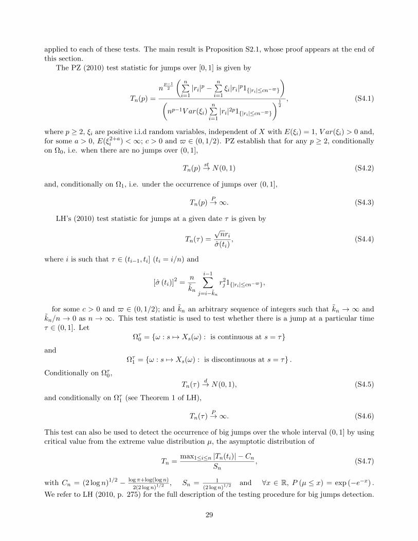
The PZ (2010) test statistic for jumps over [0, 1] is given by

Tn(p) =

np−1

2

(n∑i=1|ri|p −

n∑i=1

ξi|ri|p1|ri|≤cn−$

)(np−1V ar(ξi)

n∑i=1|ri|2p1|ri|≤cn−$

) 12

, (S4.1)

where p ≥ 2, ξi are positive i.i.d random variables, independent of X with E(ξi) = 1, V ar(ξi) > 0 and,for some a > 0, E(ξ2+a

i ) <∞; c > 0 and $ ∈ (0, 1/2). PZ establish that for any p ≥ 2, conditionallyon Ω0, i.e. when there are no jumps over (0, 1],

Tn(p)st→ N(0, 1) (S4.2)

and, conditionally on Ω1, i.e. under the occurrence of jumps over (0, 1],

Tn(p)P→∞. (S4.3)

LH’s (2010) test statistic for jumps at a given date τ is given by

Tn(τ) =

√nri

σ(ti), (S4.4)

where i is such that τ ∈ (ti−1, ti] (ti = i/n) and

[σ (ti)]2 =

n

kn

i−1∑j=i−kn

r2j1|ri|≤cn−$,

for some c > 0 and $ ∈ (0, 1/2); and kn an arbitrary sequence of integers such that kn → ∞ andkn/n → 0 as n → ∞. This test statistic is used to test whether there is a jump at a particular timeτ ∈ (0, 1]. Let

Ωτ0 = ω : s 7→ Xs(ω) : is continuous at s = τ

andΩτ

1 = ω : s 7→ Xs(ω) : is discontinuous at s = τ .

Conditionally on Ωτ0 ,

Tn(τ)d→ N(0, 1), (S4.5)

and conditionally on Ωτ1 (see Theorem 1 of LH),

Tn(τ)P→∞. (S4.6)

This test can also be used to detect the occurrence of big jumps over the whole interval (0, 1] by usingcritical value from the extreme value distribution µ, the asymptotic distribution of

Tn =max1≤i≤n |Tn(ti)| − Cn

Sn, (S4.7)

with Cn = (2 log n)1/2 − log π+log(logn)

2(2 logn)1/2 , Sn = 1

(2 logn)1/2 and ∀x ∈ R, P (µ ≤ x) = exp (−e−x) .

We refer to LH (2010, p. 275) for the full description of the testing procedure for big jumps detection.

29

To define the bootstrap test statistics, let the local Gaussian bootstrap sample be r∗i : i =1, . . . , n, with

r∗i =√vni · ηi,

where ηi is i.i.d N(0, 1) independent of the data and vni is a local volatility estimator. We define thebootstrap version of PZ’s test statistic Tn(p) in (S4.1) by

T ∗n(p) =

np−1

2

(n∑i=1|r∗i |p −

n∑i=1

ζi|r∗i |p1|r∗i |≤cn−$

)(np−1V ar(ζi)

n∑i=1|r∗i |2p1|r∗i |≤cn−$

) 12

, (S4.8)

where ζi is an i.i.d sequence of positive random variables which is independent of the data, ξi and ηi,and has the same distribution as ξi.

The bootstrap version of LH’s test statistic Tn(τ) in (S4.4) for jump at date τ ∈ (ti−1, ti] is

T ∗n(τ) =

√nr∗i

σ∗(ti)=

√nvni

σ∗ (ti)ηi, (S4.9)

where [σ∗ (ti)]2 is the bootstrap analog of [σ (ti)]

2 , obtained by replacing rm by r∗m in [σ (ti)]2 . More

precisely,

[σ∗ (ti)]2 =

n

kn

i−1∑j=i−kn

r∗2

j 1|r∗j |≤cn−$.

We establish the bootstrap validity for the PZ and LH tests under the following Conditions A(PZ-p) and A(LH-τ), respectively. These conditions are the analogue to Condition A in the main textunder which the validity of the local Gaussian bootstrap is established for the BN-S jump test.

Condition A(PZ-p)

(i) There exists δ > p such that,

$ <1

2− 1

2δand ∀` ∈ (0, δ], n−1+`

n∑i=1

(vni )`P→∫ 1

0σ2`u du.

(ii)

n−1+2pn∑i=1

(vni )2p = OP (1).

Condition A(LH-τ)

(i) As n→∞, kn →∞ and kn/n→ 0.

(ii) For j = i− kn, . . . , i− 1, nvnjP→ σ2

τ as n→∞ and 1kn

∑i−1

j=i−kn

(nvnj

)2= Op (1), where i is such

that τ ∈ (ti−1, ti].

Similarly to Condition A, these conditions apply to the sequence of local volatility estimates andso long as these conditions are satisfied both under the null and the alternative, the bootstrap testcontrols size under the null and is consistent under the alternative. The main result is as follows.

Proposition S4.1 Let X be an Ito semimartingale defined by (1) and satisfying Assumption (H-2).

30

(i) If Condition A(PZ-p) holds for some p ≥ 2, then

T ∗n(p)d∗→ N(0, 1),

in probability.

(ii) If Condition A(LH-τ) holds for some τ ∈ (0, 1], then

T ∗n(τ)d∗→ N (0, 1) ,

in probability.

Before providing the proof of this proposition, we make the following remarks.

Remark 1 The bootstrap version T ∗n(τ) of LH’s test statistic can be used to detect the occurrence ofbig jumps over a fixed time interval such as [0, 1]. A sufficient condition is that Condition A(LH-τ)holds for all τ ∈ (0, 1]. Under this condition and because the ηi’s are independent conditionally on thedata, the T ∗n(ti) are also conditionally independent and asymptotically standard normal over the entireinterval. In this case, the bootstrap can be used to compute the critical values of LH’s (2010) big jumptest. In particular, we reject the absence of jumps at any given time ti whenever the absolute value ofTn (ti) exceeds q∗αSn + Cn, where q∗α is the α quantile of the bootstrap distribution of

T ∗n =max1≤i≤n |T ∗n(ti)| − Cn

Sn. (S4.10)

Note that the test statistic Tn can be used directly to test for occurrence of jumps over long timeintervals. This has been highlighted by Aıt-Sahalia and Jacod (2014, Chap. 10). In this case, criticalvalues from the extreme value distribution µ or from the bootstrap distribution of T ∗n can be used.

Remark 2 A bootstrap version of the QQ-plot test for small jumps can also be obtained by com-paring the empirical quantiles of Tn(ti) : i = kn, . . . , n to those of the bootstrap samples T ∗n(ti) :i = kn, . . . , n. The bootstrap samples replace the artificial samples drawn from the standard normaldistribution originally proposed by Lee and Hannig (2010).

Remark 3 If we implement the bootstrap jump tests of PZ and LH with vni based on thresholding (asdiscussed in Section 3.2 for the BN-S test), the truncation parameter, say $′, used for the bootstrapdata generating process need not be equal to $ - the truncation parameter used in the test statistics. Inparticular, to satisfy Condition A(PZ-p), one can first choose $ ∈ (0, 1/2) and then, set $′ such that

max(

2p−14p−r ,

δ−12δ−r

)≤ $′ < 1

2 for some δ > max(p, 1

1−2$

). We can show that under these conditions,

Condition A(PZ-p) holds by Theorem 9.4.1 of Jacod and Protter (2012). While these restrictions on$ and $′ matter for Condition A(PZ-p) to be satisfied under the alternative of occurrence of jumps,they are immaterial under the null of no jumps since this condition is fulfilled for any choice $ and$′ in (0, 1/2) . Given Theorem 9.3.2 of Jacod and Protter (2012) and their comments leading to thattheorem, we can claim that Condition A(LH-τ) is also fulfilled for a local volatility estimate based onthresholding so long as we maintain that the volatility process σ2

s is continuous at s = τ . The validityof the test over the full range [0, 1] is therefore guaranteed under the common assumption that the priceand volatility processes do not jump at the same time.

Remark 4 We have implemented the bootstrap versions of the PZ (2010) and LH (2010) tests inunreported simulation results using the same data generating processes as in the main text. Our findingsare as follows: (1) the PZ (2010) is slightly oversized under the null of no jumps and the local Gaussian

31

bootstrap helps alleviate these finite size distortions without sacrificing power; (2) the bootstrap big-jump LH (2010) test outperforms the original test of LH (2010) by showing a lower probability of globalmisclassification. Specifically, the bootstrap version of the test has a lower probability of global spuriousdetection of jumps than the original test while both tests have the same probability of global failure todetect jumps. (3) the small-jump LH test also has a low probability of global spurious detection ofjumps that ranges between between 3.65% for n = 78 and 3.47% for n = 576, although not as low asthat of the bootstrap big-jump LH (2010). Its probability of global success in detecting actual jumps ismuch smaller than both versions of the big-jump LH test when the alternative is finite activity jumpsbut it dominates any of these two tests when there are infinite activity jumps. This is as expectedsince the small-jump test of LH (2010) is especially designed to detect small jumps; (4) The big-jumptest over long time intervals using directly (S4.7) (Aıt-Sahalia and Jacod (2014, Chap. 10)) has alarge size distortion under the null of no jumps that decays slowly from 63.14% (n = 78) to 58.09%(n = 576). Interestingly, the bootstrap version of this test, with rejection rates under the null from3.14% to 5.56%, corrects this size distortion while showing reasonable power.

Proof of Proposition S4.1: (i) Let

a∗n = np−1

2

(n∑i=1

|r∗i |p −n∑i=1

ζi|r∗i |p1|r∗i |≤cn−$

), d∗n = np−1V ar(ζi)

n∑i=1

|r∗i |2p1|r∗i |≤cn−$,

so that T ∗n(p) = a∗n/√d∗n. Let

a∗1n = np−1

2

n∑i=1

|r∗i |p(1− ζi), a∗2n = np−1

2

n∑i=1

ζi|r∗i |p1|r∗i |≤cn−$.

Clearly, a∗n = a∗1n + a∗2n. We will show that (a) a∗2n = oP ∗(1), in probability, and that d∗n is positivewith probability approaching one so that T ∗n(p) = a∗1n/

√d∗n + oP ∗(1). Let vn = V ar∗(a∗1n) and

S∗n = a∗1n/√vn. We complete the proof of statement (i) by showing that: (b) S∗n

d∗→ N(0, 1), in

probability and (c) d∗n − vnP ∗→ 0, in probability.

(a) We have

|a∗2n| ≤ np−1

2

n∑i=1

|ζi||r∗i |p1|r∗i |≤cn−$ ≤ np−1

2

n∑i=1

ζi|r∗i |p|r∗i |l

cln−$l,

for all l > 0. Hence, using the fact that r∗i =√vni · ηi, ηi ∼ N(0, 1), we have that

E∗|a∗2n| ≤ C · np−1

2+l$

n∑i=1

(vni )p+l2 = C · n

12

+l$− l2 · n−1+ p+l

2

n∑i=1

(vni )p+l2 ,

where C > 0 is a generic constant. Choosing l close enough to δ so that $ < 12 −

12l ensures, using

Condition A(PZ-p)-(i) that a∗2n = oP ∗(1) in probability. The positivity of d∗n is proven in part (c)below.

(b) Simple calculations show that vn = µ2pV ar(ζi)n−1+p

∑ni=1(vni )p which, under Condition

A(PZ-p)-(i) converges in probability to the almost surely positive random variable µ2pV ar(ζi)∫ 1

0 σ2pu du.

We can therefore focus on establishing the conditions that ensure that a∗1n is asymptotically normal.Note that

a∗1n =n∑i=1

np−1

2 |r∗i |p(1− ζi) =n∑i=1

np−1

2 (vni )p2 |ηi|p(1− ζi).

32

By the independence across i of the terms in this summation and the fact that E∗(|ηi|p(1− ζi)) = 0,it suffices to verify the Lyapunov condition to conclude (b). That is, we show that there exists ν > 0such that

n∑i=1

E∗∣∣∣n p−1

2 |r∗i |p(1− ζi)∣∣∣2+ν

= oP ∗(1),

in probability. It is not hard to see that

n∑i=1

E∗∣∣∣n p−1

2 |r∗i |p(1− ζi)∣∣∣2+ν

= C · n−ν/2 · n−1+p(1+ν/2)n∑i=1

(vni )p(1+ν/2).

Again, one can choose ν > 0 so that p < p(1 + ν/2) ≤ δ and use Condition A(PZ-p)-(i) to conclude.(c) Note that

d∗n = np−1V ar(ζi)

n∑i=1

|r∗i |2p − np−1V ar(ζi)

n∑i=1

|r∗i |2p1(|r∗i |>cn−$) ≡ d∗1n + d∗2n.

It is not hard to prove by following similar steps as those in (a) above that d∗2n = oP ∗(1) in probability.

Hence, it suffices to show that d∗1n − vnP ∗→ 0, in probability. Note that E∗(d∗1n) = vn and it suffices to

show that V ar∗(d∗1n) = oP (1) to conclude (d). We have:

V ar∗(d∗1n) = V ar(|ηi|2p

)[V ar(ζi)]

2n−1n−1+2pn∑i=1

(vni )2p = oP (1),

thanks to Condition A(PZ-p)-(ii). The positivity of d∗n also follows.

(ii) Since ηi ∼ N(0, 1) and is independent of the data, it suffices to show that

√nvni

σ∗(ti)

P ∗→ 1 in

probability and, under Condition A(LH-τ), it suffices to show that [σ∗ (ti)]2 P ∗→ σ2

τ , in probability. Forthis, we show that

E∗(

[σ∗ (ti)]2 − σ2

τ

)P→ 0 and V ar∗

([σ∗ (ti)]

2 − σ2τ

)P→ 0.

The following inequality (proven by successive applications of the Holder inequality with Holderconjugates q/p > 1 and q/(q− p)) and the Markov inequality (with exponent 2q) implies that for anyq > p > 0,

E∗(|√nr∗j |2p1|r∗j |≤cn−$

)≤ K

(nvnj

)qn−2(q−p)(1/2−$), (S4.11)

where K is a positive constant. To show that E∗(

[σ∗ (ti)]2)

P→ σ2τ , it suffices to show that

E∗

n

kn

i−1∑j=i−kn

r∗2

j 1|r∗j |≤cn−$

P→ 0,

since

E∗

n

kn

i−1∑j=i−kn

r∗2

j

=1

kn

i−1∑j=i−kn

(nvnj )P→ σ2

τ .

33

Note that

E∗

n

kn

i−1∑j=i−kn

r∗2

j 1|r∗j |≤cn−$

=1

kn

i−1∑j=i−kn

E∗(

(√nr∗j )

21|r∗j |≤cn−$)

≤ K

1

kn

i−1∑j=i−kn

(nvnj

)q︸ ︷︷ ︸

=Op(1)

n−2(q−1)(1/2−$)︸ ︷︷ ︸=o(1)

,

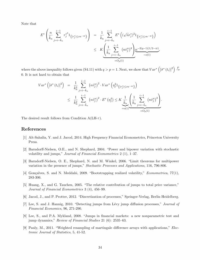
where the above inequality follows given (S4.11) with q > p = 1.Next, we show that V ar∗(

[σ∗ (ti)]2)

P→0. It is not hard to obtain that

V ar∗(

[σ∗ (ti)]2)

=1

k2n

i−1∑j=i−kn

(nvnj

)2 · V ar∗ (η2j 1|r∗j |≤cn−$

)

≤ 1

k2n

i−1∑j=i−kn

(nvnj

)2 · E∗ (η4j

)≤ K 1

kn︸︷︷︸=o(1)

1

kn

i−1∑j=i−kn

(nvnj

)2︸ ︷︷ ︸

=Op(1)

.

The desired result follows from Condition A(LH-τ).

References

[1] Aıt-Sahalia, Y. and J. Jacod, 2014. High Frequency Financial Econometrics, Princeton UniversityPress.

[2] Barndorff-Nielsen, O.E., and N. Shephard, 2004. “Power and bipower variation with stochasticvolatility and jumps,” Journal of Financial Econometrics 2 (1), 1–37.

[3] Barndorff-Nielsen, O. E., Shephard, N. and M. Winkel, 2006. “Limit theorems for multipowervariation in the presence of jumps,” Stochastic Processes and Applications, 116, 796-806.

[4] Goncalves, S. and N. Meddahi, 2009. “Bootstrapping realized volatility,” Econometrica, 77(1),283-306.

[5] Huang, X., and G. Tauchen, 2005. “The relative contribution of jumps to total price variance,”Journal of Financial Econometrics 3 (4), 456–99.

[6] Jacod, J., and P. Protter, 2012. “Discretization of processes,” Springer-Verlag, Berlin Heidelberg.

[7] Lee, S. and J. Hannig, 2010. “Detecting jumps from Levy jump diffusion processes,” Journal ofFinancial Economics, 96, 271-290.

[8] Lee, S., and P.A. Mykland, 2008. “Jumps in financial markets: a new nonparametric test andjump dynamics,” Review of Financial Studies 21 (6): 2535–63.

[9] Pauly, M., 2011. “Weighted resampling of martingale difference arrays with applications,” Elec-tronic Journal of Statistics, 5, 41-52.

34

[10] Podolskij, M., and D. Ziggel, 2010. “New tests for jumps in semimartingale models,”StatisticalInference for Stochastic Processes 13(1), 15-41.

[11] Shao, X., 2010. “The dependent wild bootstrap,” Journal of the American Statistical Association,105, 218-235.

35