Bootstrap and Jackknife - Harvard Universitystat221/spring-2006/intro/bootstrap.pdf · Bootstrap and Jackknife • in Statistics, we deal with the difﬁculty of ﬁnding the distribution

[email protected] Stat221 www.fas.harvard.edu/˜stat221'

&

$

%

Bootstrap and Jackknife

• in Statistics, we deal with the difficulty of finding the distribution /

standard errors of uncommon test statistics

• Bootstrap and Jackknife are general recipes to attack this problem

• Bootstrap offers much more, as we will find out

April 30, 2006 c© 2006 - Gopi Goswami ([email protected] ) Page 1


&

$

%

Plug-in Estimators I

• we have independent observations Xn := (X1, X2, . . . , Xn) from an

unknown density f(·) with c.d.f. F (·)

• want to estimate an interesting feature of the distribution θ = T (F ), where

T (·) is a function of the c.d.f., e.g.,

– mean: if θ = E(X1) =∫xf(x) dx =

∫x dF (x) then T (G) =

∫x dG(x),

where G(·) is any c.d.f.

– median: if θ = F−1(0.5) then T (F ) = G−1(0.5), where G(·) is any c.d.f.

• say Fn(·) is the empirical c.d.f. of the data Xn, i.e., Fn(·) puts mass 1/n on

each of the data points Xi, i = 1, 2, . . . , n

• then one could use the plug-in estimator of θ: θn := T (Fn) = t(Xn), e.g.,

– mean: if T (F ) =∫x dG(x) then

T (Fn) =∫x dFn(x) = 1

n

∑ni=1Xi = Xn = t(Xn), the sample mean

– median: if T (G) = G−1(0.5) then T (Fn) = F−1n (0.5) = t(Xn), the sample

median



&

$

%

Plug-in Estimators II

• plug-in estimator of the variance:

θ = E(X1 − E(X1))2 = E(X2

1 ) − (E(X1))2

=

∫x2 dF (x) −

{∫x dF (x)

}2

= T (F ) and hence

T (Fn) =

∫x2 dFn(x) −

{∫x dFn(x)}

2

}=

1

n

n∑

i=1

X2i −

{1

n

n∑

i=1

Xi

}2

=1

n

n∑

i=1

(Xi − Xn)2 =

n− 1

ns2n

• note here E(T (Fn)) = n−1n E(s2n) = n−1

n θ 6= θ, i.e., the plug-in estimator is

biased



&

$

%

Bootstrap Principle

• inference on θ is usually based on the distribution of T (Fn) = t(Xn) or of

R(Xn, F ) := T ( bFn)−T (F )

S( bFn), where S(·) is a functional, which estimates

V ar(T (Fn)) or for other forms of R(Xn, F )

• both of the above distributions may be intractable and it also may depend

on the unknown F (·)

• bootstrap provides a way out using random bootstrap samples or pseudo-data

sets denoted by X ?n := (X?

1 , X?2 , . . . , X

?n), we’ll see how to generate these in a

bit

• let F ?n(·) be the empirical c.d.f. of the data X ?n , i.e., F ?n(·) puts mass 1/n on

each of the data points X?i , i = 1, 2, . . . , n

• since X ?n is randomly generated, F ?n(·) is a random variable

• now the bootstrap principle says that approximate the distribution of

– T (Fn) = t(Xn) by the bootstrap distribution of T (F ?n) = t(X ?n)

– R(Xn, F ) by the bootstrap distribution of R(X ?n , Fn)



&

$

%

Bootstrap Sample or Pseudo-data Set

• Non-parametric Bootstrap:

data world: Xn := (X1, X2, . . . , Xn), Xii.i.d.∼ F (·), i = 1, 2, . . . , n

bootstrap world: X ?n := (X?

1 , X?2 , . . . , X

?n), X

?ii.i.d.∼ Fn(·), i = 1, 2, . . . , n

here the pseudo-data set is a simple random sample of size n with

replacement from Xn := (X1, X2, . . . , Xn)

• Parametric Bootstrap: let θ and θn be a parameter and it’s reasonable

estimator below (may not necessarily be the plug-in estimator!)

data world: Xn := (X1, X2, . . . , Xn), Xii.i.d.∼ F (·, θ), i = 1, 2, . . . , n

bootstrap world: X ?n := (X?

1 , X?2 , . . . , X

?n), X

?ii.i.d.∼ F (·, θn), i = 1, 2, . . . , n

here the pseudo-data set is a random sample of size n from F (·, θn)



&

$

%

Bootstrap Distribution

• note that both in non-parametric and in parametric bootstrap, the bootstrap

samples are generated “using” the observed data Xn, i.e., conditioned on Xn

• for non-parametric bootstrap the number of possible bootstrap samples is

nn(≈ ∞, for large n)

• for parametric bootstrap the number of possible bootstrap samples is ∞

• since it’s not possible or efficient to consider all possible bootstrap samples

we work with B-many bootstrap samples

X ?n,b = {X?

1,b, X?2,b, . . . , X

?n,b}, b = 1, 2, . . . , B

• then the bootstrap distribution of T (F ?n) = t(X ?n) and of R(X ?

n , Fn) can be

approximated by the following empirical distributions of

G?B,T (·) is the c.d.f. of{T (F ?n,b) = t(X ?

n,b) | b = 1, 2, . . . , B}

and

G?B,R(·) is the c.d.f. of{R(X ?

n,b, Fn) | b = 1, 2, . . . , B}



&

$

%

Bootstrap Standard Error

• let us consider the problem of estimating θ = T (F ) by the plug-in estimator

T (Fn) = t(Xn), say

• interested in the standard error of the estimator T (Fn), i.e., we want to

estimate

√V arF (T (Fn)) =

√V arF (t(Xn))

• use the sample standard deviation of the c.d.f. G?B,T (·) or of the (bootstrap

sample) evaluations {t(X ?n,b) | b = 1, 2, . . . , B} as an estimator of√

V arF (T (Fn)) =√V arF (t(Xn)):

seboot,B(t) =

{1

B − 1

B∑

b=1

(t(X ?

n,b) − t?B)2

}1/2

where t?B =1

B

B∑

b=1

t(X ?n,b)



&

$

%

Non-parametric Bootstrap: Regression I

• the model: Yi = XTi β + εi, i = 1, 2, . . . , n

• want the standard error of βOLS

• define Zi := (XTi , Yi), i = 1, 2, . . . , n

• generate B-many pseudo-data sets Z?n,b = {Z?1,b, Z

?2,b, . . . , Z

?n,b} by sampling

with replacement from {Z1, Z2, . . . , Zn} randomly

• for b = 1, 2, . . . , B, regress (OLS) {Y ?i,b | i = 1, 2, . . . , n} on

{X?Ti,b | i = 1, 2, . . . , n} to get β?b = t(Z?

n,b), say

• now compute bootstrap standard error seboot,B(t), to get the standard error

of βOLS

• this is also called paired bootstrapping



&

$

%

Non-parametric Bootstrap: Regression II

• the model: Yi = XTi β + εi, i = 1, 2, . . . , n

• want standard error of βOLS

• the (OLS) estimated model: Yi = XTi βOLS + εi, i = 1, 2, . . . , n

• generate pseudo-data sets E?n,b = {ε?1,b, ε?2,b, . . . , ε

?n,b} by sampling with

replacement from {ε1, ε2, . . . , εn} randomly

• now define Z?i = (Y ?i := XTi βOLS + ε?i , Xi) and form

Z?n,b = {Z?1,b, Z

?2,b, . . . , Z

?n,b}

• for b = 1, 2, . . . , B, regress (OLS) {Y ?i,b | i = 1, 2, . . . , n} on

{Xi | i = 1, 2, . . . , n} to get β?b = t(Z?n,b), say


of βOLS

• this is also called bootstrapping the residuals



&

$

%

Parametric Bootstrap: Gamma model

• the model: Yii.i.d.∼ Γ(α, 1), i = 1, 2, . . . , n

• want the standard error of αMLE

• note αMLE is gotten by numerically solving the “score equation”

• generate B-many pseudo-data sets Y?n,b = {Y ?1,b, Y?2,b, . . . , Y

?n,b} by drawing

independently from the distribution Γ(αMLE, 1)


of αMLE

• this is preferable than the non-parametric version if we strongly believe that

the data generation process, which is a Γ(·, 1) distribution here



&

$

%

Bootstrap Estimate Of Bias


T (Fn) = t(Xn) = θn

• want to estimate the bias in estimation:

EF (θn) − θ = EF (t(Xn)) − θ = EF (T (Fn)) − T (F ) = R(Xn, F ), say

• we estimate it by:

R(X ?n , Fn) = E bFn

(T (F ?n)) − T (Fn) = E bFn(t(X ?

n)) − t(Xn) = E bFn(θ?n) − θn

• use the c.d.f. G?B,R(·) or the (bootstrap sample) evaluations

{t(X ?n,b) = θ?n,b | b = 1, 2, . . . , B} to approximate by E bFn

(T (F ?n)) − θn

biasboot,B(t) :=1

B

B∑

b=1

t(X ?n,b) − t(Xn) =

1

B

B∑

b=1

θ?n,b − θn



&

$

%

Jackknife I• we have independent observations Xn := (X1, X2, . . . , Xn) from an

unknown density f(·) with c.d.f. F (·),

• consider the problem of estimating θ = T (F ) using θn = t(Xn)

• form the “leave-one” data sets:

X(−i) := {Xj | j = 1, 2, . . . , n, j 6= i}, i = 1, 2, . . . , n

• define θ(−i) = t(X(−i)), i = 1, 2, . . . , n and θ(·) = 1n

∑ni=1 θ(−i)

• then the Jackknife estimate of the bias EF (θn) − θ = EF (t(Xn)) − θ is given

by:

biasjack(t) = (n− 1)(θ(·) − θn)



&

$

%

Jackknife II• then the Jackknife estimate of the standard error√

V arF (θn) =√V arF (t(Xn)) is given by:

sejack(t) =

{n− 1

n

n∑

i=1

(θ(−i) − θ(·)

)2}1/2

• why do the formulas for biasjack(t) and sejack(t) make sense?

– define the pseudo-values θi := nθn − (n− 1)θ(−i), i = 1, 2, . . . , n and their

mean ¯θ = 1

n

∑ni=1 θi

– now note,

biasjack(t) = (n− 1)(θ(·) − θn) = θn −¯θ and

sejack(t) =

{n− 1

n

n∑

i=1

(θ(−i) − θ(·)

)2}1/2

=

{1

n(n− 1)

n∑

i=1

(θi −

¯θ)2

}1/2

(1)



&

$

%

Jackknife III• note if θn = Xn, the sample mean then θi = Xi, i = 1, 2, . . . , n and ¯

θ = Xn

• here the above formulas in equation (1) become

biasjack(t) = θn −¯θ = 0 and

sejack(t) =

{1

n(n− 1)

n∑

i=1

(θi −

¯θ)2

}1/2

=

{1

n(n− 1)

n∑

i=1

(Xi − Xn

)2

}1/2

• thus the formulas in equation (1) “does the right thing” in case of θn = Xn

• hope is they will do a good job for a general statistic θn as well



&

$

%

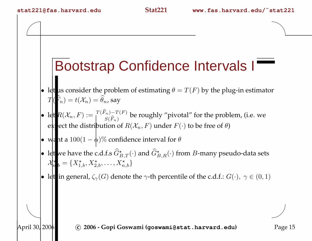
Bootstrap Confidence Intervals I


T (Fn) = t(Xn) = θn, say

• let R(Xn, F ) := T ( bFn)−T (F )

S( bFn)be roughly “pivotal” for the problem, (i.e. we

expect the distribution of R(Xn, F ) under F (·) to be free of θ)

• want a 100(1 − α)% confidence interval for θ

• let we have the c.d.f.s G?B,T (·) and G?B,R(·) from B-many pseudo-data sets

X ?n,b = {X?

1,b, X?2,b, . . . , X

?n,b}

• let, in general, ζγ(G) denote the γ-th percentile of the c.d.f.: G(·), γ ∈ (0, 1)



&

$

%

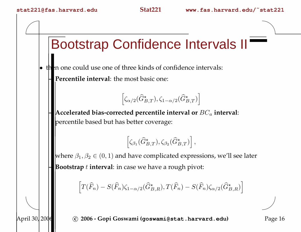
Bootstrap Confidence Intervals II

• then one could use one of three kinds of confidence intervals:

– Percentile interval: the most basic one:

[ζα/2(G

?B,T ), ζ1−α/2(G

?B,T )

]

– Accelerated bias-corrected percentile interval or BCa interval:

percentile based but has better coverage:

[ζβ1

(G?B,T ), ζβ2(G?B,T )

],

where β1, β2 ∈ (0, 1) and have complicated expressions, we’ll see later

– Bootstrap t interval: in case we have a rough pivot:

[T (Fn) − S(Fn)ζ1−α/2(G

?B,R), T (Fn) − S(Fn)ζα/2(G

?B,R)

]



&

$

%

Percentile Interval I• H(·) is a continuous and symmetric (around 0) distribution

• let ψ(·) be a continuous, strictly increasing transformation such that

ψ(θn) − ψ(θ) ∼ H(·), e.g. ψ(·) could be a normalizing transformation

• then we have, by symmetry of H(·):

Phζα/2(H) ≤ ψ(bθn) − ψ(θ) ≤ ζ1−α/2(H)

i= 1 − α (2)

=⇒ Phψ

−1(−ζ1−α/2(H) + ψ(bθn)) ≤ θ ≤ ψ−1(−ζα/2(H) + ψ(bθn))

i= 1 − α

=⇒ Phψ

−1(ζα/2(H) + ψ(bθn)) ≤ θ ≤ ψ−1(ζ1−α/2(H) + ψ(bθn))

i= 1 − α (3)

• using the bootstrap principle on equation (2) we have,

P?

hζα/2(H) ≤ ψ(bθ?

n) − ψ(bθn) ≤ ζ1−α/2(H)i

≈ 1 − α

=⇒ P?

hψ

−1(ζα/2(H) + ψ(bθn)) ≤ bθ?n ≤ ψ

−1(ζ1−α/2(H) + ψ(bθn))i≈ 1 − α (4)



&

$

%

Percentile Interval II• compare equations (3), (4) and note that their upper and lower limits

coincide

• but from equation (4), we can take

ψ−1(ζα/2(H) + ψ(bθn)) ≈ ζα/2( bG?

B,T ) and

ψ−1(ζ1−α/2(H) + ψ(bθn)) ≈ ζ1−α/2( bG?

B,T )

• thus the required interval for 100(1 − α)% confidence interval for θ is

hζα/2( bG?

B,T ), ζ1−α/2( bG?B,T )

i

• note explicit specification of the transformation ψ(·) is not necessary



&

$

%

BCa Interval I

• let ψ(·) be a continuous, strictly increasing transformation and a, b ∈ R1 such

that 1 + aψ(θ) > 0 and

U :=ψ(bθn) − ψ(θ)

1 + aψ(θ)+ b ∼ Normal1(0, 1)

• note a = b = 0 takes us back to the simple percentile method

• with zγ denote the γ-th percentile of the Normal1(0, 1) distribution we

have,

Pˆzα/2 ≤ U ≤ z1−α/2

˜= 1 − α (5)

=⇒ Phk1(a, b, 1 − α/2, bθn) ≤ θ ≤ k1(a, b, α/2, bθn)

i= 1 − α, where (6)

k1(a, b, γ, bθn) = ψ−1

ψ(bθn) +

(b− zγ)[1 + aψ(bθn)]

1 − a(b− zγ)

!

(7)



&

$

%

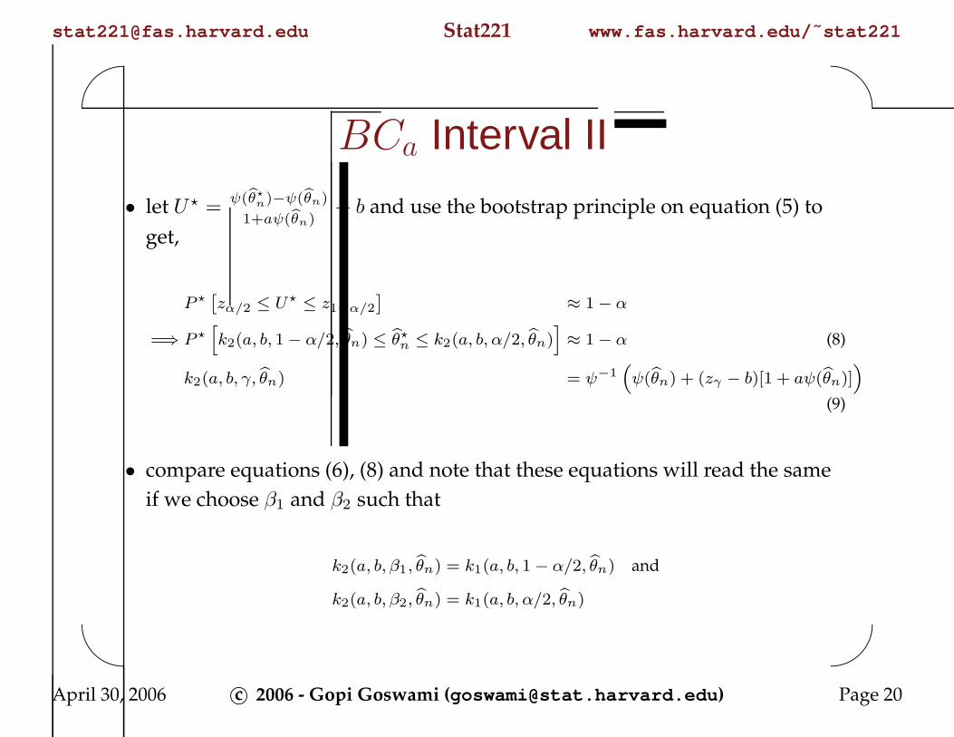
BCa Interval II

• let U? =ψ(bθ?

n)−ψ(bθn)

1+aψ(bθn)+ b and use the bootstrap principle on equation (5) to

get,

P ?ˆzα/2 ≤ U? ≤ z1−α/2

˜≈ 1 − α

=⇒ P ?hk2(a, b, 1 − α/2, bθn) ≤ bθ?

n ≤ k2(a, b, α/2, bθn)i≈ 1 − α (8)

k2(a, b, γ, bθn) = ψ−1

“ψ(bθn) + (zγ − b)[1 + aψ(bθn)]

”

(9)

• compare equations (6), (8) and note that these equations will read the same

if we choose β1 and β2 such that

k2(a, b, β1, bθn) = k1(a, b, 1 − α/2, bθn) and

k2(a, b, β2, bθn) = k1(a, b, α/2, bθn)



&

$

%

BCa Interval III

• choice of β1 boils down to (below Φ(·) is the c.d.f. of the Normal1(0, 1)

distribution):

ψ−1

“ψ(bθn) + (zβ1

− b)[1 + aψ(bθn)]”

= ψ−1

ψ(bθn) +

(b− z1−α/2)[1 + aψ(bθn)]

1 − a(b− z1−α/2)

!

⇐⇒zβ1− b =

(b− z1−α/2)

1 − a(b− z1−α/2)⇐⇒ β1 = Φ

b+

b− z1−α/2

1 − a(b− z1−α/2)

!

• similarly, we get, β2 = Φ(b+

b−zα/2

1−a(b−zα/2)

)

• but from equation (8), we can take

k2(a, b, β1, bθn) ≈ ζβ1( bG?

B,T ) and

k2(a, b, β2, bθn) ≈ ζβ2( bG?

B,T )



&

$

%

BCa Interval IV

• thus the required interval for 100(1 − α)% confidence interval for θ is

hζβ1

( bG?B,T ), ζβ2

( bG?B,T )

i

• note, both β1 and β2 depends on a and b and usually one takes

b = Φ−1(G?B,T (θn)

)and

a =

∑ni=1 τ

3i

6 (∑ni=1 τ

2i )

3/2where

τi = θ(·) − θ(−i) remember jackknife!

• note explicit specification of the transformation ψ(·) is not necessary

• this method just “corrects the percentiles”, i.e. uses β1 and β2 instead of

1 − α2 and α/2 from the percentile method



&

$

%

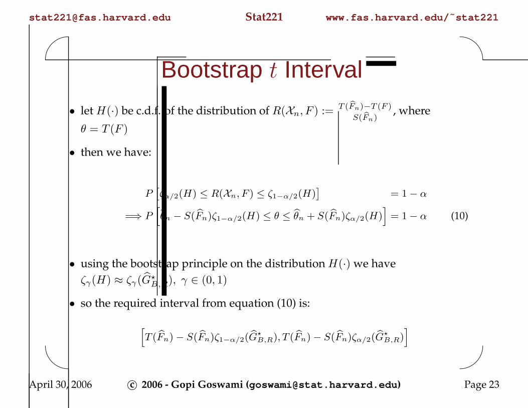
Bootstrap t Interval

• let H(·) be c.d.f. of the distribution of R(Xn, F ) := T ( bFn)−T (F )

S( bFn), where

θ = T (F )

• then we have:

Pˆζα/2(H) ≤ R(Xn, F ) ≤ ζ1−α/2(H)

˜= 1 − α

=⇒ Ph

bθn − S( bFn)ζ1−α/2(H) ≤ θ ≤ bθn + S( bFn)ζα/2(H)i

= 1 − α (10)

• using the bootstrap principle on the distribution H(·) we have

ζγ(H) ≈ ζγ(G?B,R), γ ∈ (0, 1)

• so the required interval from equation (10) is:

hT ( bFn) − S( bFn)ζ1−α/2( bG?

B,R), T ( bFn) − S( bFn)ζα/2( bG?B,R)

i



&

$

%

Bootstrap vs. Jackknife I

• the set up (from problem 4 on problem set 5):

– let we have Xn := (X1, X2, . . . , Xn)i.i.d.∼ f(·) with c.d.f. F (·)

– let we have a linear statistic of the form θn = µ+ 1n

∑ni=1 α(Xi)

• you showed that for this statistic that the variance of the ideal bootstrap

estimator V ar bFn(θ?n) and that of the jackknife estimator V arjack(θ

?n) differ

by only a factor of n−1n

• let we have a quadratic statistic of the form

θn = µ+ 1n

∑1≤i≤n α(Xi) + 1

n2

∑1≤i<j≤n β(Xi, Xj)

• the ideal bootstrap bias estimate, E bFn(θ?n) − θn and the jackknife bias

estimate, biasjack(t) differ by only a factor of n−1n



&

$

%

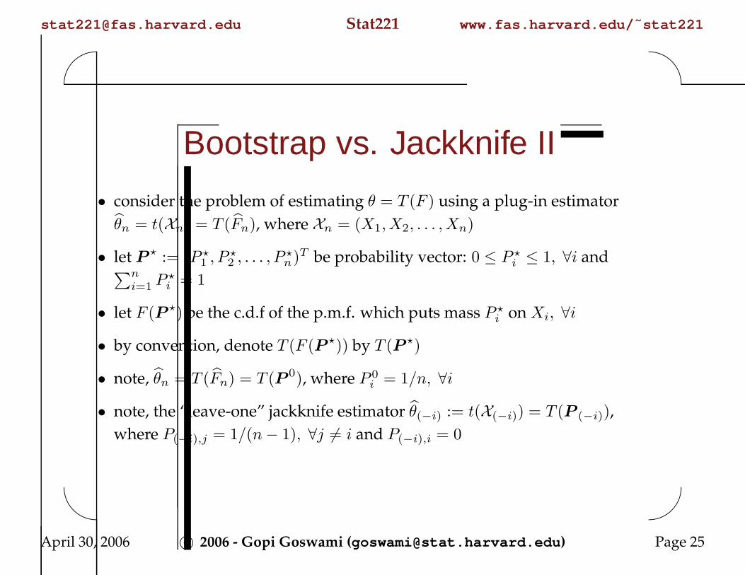
Bootstrap vs. Jackknife II

• consider the problem of estimating θ = T (F ) using a plug-in estimator

θn = t(Xn) = T (Fn), where Xn = (X1, X2, . . . , Xn)

• let P ? := (P ?1 , P?2 , . . . , P

?n)T be probability vector: 0 ≤ P ?i ≤ 1, ∀i and∑n

i=1 P?i = 1

• let F (P ?) be the c.d.f of the p.m.f. which puts mass P ?i on Xi, ∀i

• by convention, denote T (F (P ?)) by T (P ?)

• note, θn = T (Fn) = T (P 0), where P 0i = 1/n, ∀i

• note, the “leave-one” jackknife estimator θ(−i) := t(X(−i)) = T (P (−i)),

where P(−i),j = 1/(n− 1), ∀j 6= i and P(−i),i = 0



&

$

%

Bootstrap vs. Jackknife III

• consider the random variable P ? such that

n · P ? ∼ Multinomial(n,P 0)

• recall, a non-parametric bootstrap sample or pseudo-data set

X ?n := (X?

1 , X?2 , . . . , X

?n) is generated by X?

ii.i.d.∼ Fn(·), i = 1, 2, . . . , n

• the above procedure is equivalent to the following, which uses P ?:

generate M? := n · P ? ∼ Multinomial(n,P 0)

set X ?n = {M?

i many copies of Xi}, why?

thus F ?n = F (P ?)

• thus we have, θ?n = t(X ?n) = T (F ?n) = T (F (P ?)) = T (P ?)



&

$

%

Bootstrap vs. Jackknife IV

• “jackknife is linearized bootstrap” in the following sense:

Theorem 0.1. Let us consider the problem of estimating θ = T (F ) by the plug-in

estimator T (Fn) = t(Xn) = θn. Here, θn may not a linear statistic. We know,

V arjack(t) =n− 1

n

n∑

i=1

(θ(−i) − θ(·)

)2

Let TLIN (P ?) := c0 + (P ? − P 0)TU , where∑n

i=1 Ui = 0 (so that only n among

c0,U are free to vary) be a linear statistic. So, TLIN (P ?) is a hyperplane defined

on the n-dimensional simplex,

Sn := {x ∈ Rn | 0 ≤ xi ≤ 1, i = 1, 2, . . . , n,

∑ni=1 xi = 1}. Solve for c0,U

under the n conditions T (P (i)) = θ(−i), i = 1, 2, . . . , n to get TLIN,bθn(P ?), the

“linearized” version of θ?n. Then, for the ideal bootstrap variance of TLIN,bθn(P ?),

we have

V ar(TLIN,bθn(P ?)) =

n− 1

nV arjack(t)



&

$

%

Bootstrap vs. Jackknife V

• the set up (from problem 3 on problem set 5):

– let d > 1 and X = (X1, X2, . . . , Xd)T ∼ Normald(µ, Id), where

µj = j, j = 1, 2, . . . , d and Id is the d-dimensional identity matrix

– consider n independent copies

Xi = (Xi,1, Xi,2, . . . , Xi,d)T , i = 1, 2, . . . , n of X

– let ζ1,j := V ar( 1n

∑ni=1Xi,j) and ζ2,j := V ar

(1n

∑ni=1X

2i,j

)and define

ζk := (ζk,1, ζk,2, . . . , ζk,d)T , k = 1, 2.

• note

V arF (ζboot,k,B,n) = V arF (E bFn(ζboot,k,B,n | Xn)) +EF (V ar bFn

(ζboot,k,B,n | Xn))

= V arF (ζk,n) + EF (V ar bFn(ζboot,k,B,n | Xn))

if E bFn(ζboot,k,B,n | Xn) = ζk,n



&

$

%

Bootstrap vs. Jackknife VI

• thus bootstrap introduces the extra source of variation, called the cushion

error, EF (V ar bFn(ζboot,k,B,n | Xn)) due to finite re-sampling (of size B) from

all possible bootstrap samples, see [4, Yatracos, 2002]

• the performance of ζboot,k,B,n will depend on the estimand (compare

ζboot,1,B,n and ζboot,2,B,n) and the dimension of the problem (e.g., compare

ζboot,1,B,n for different values of the underlying d) since the both of these

factors will contribute to the cushion error

• note for jackknife, the cushion error EF (V ar bFn(ζjack,k,n | Xn)) = 0, since

given a sample Xn, there is only one jackknife estimator ζjack,k,n!

• thus if we either use ζn or ζjack,k,n instead of ζboot,k,B,n, then we’ll not be

paying for the cushion error



&

$

%

Bootstrap vs. Jackknife VII

• one way to bring the cushion error down is to use a very large value of B,

especially for large dimensions, so that V ar bFn(ζboot,k,B,n | Xn) is small

• another way to would be to only use biased set of bootstrap samples for

which the F ?n(·)’s lie “close” to the Fn(·) in some sense, see [3, Hall et. al.,

1999]

• the later method is also called biased-bootstrap or b-bootstrap



&

$

%

References

[1] B. Efron. Bootstrap methods: Another look at the jackknife. The Annals of

Statistics, 7:1–26, 1979.

[2] Bradley Efron and Robert Tibshirani. An Introduction to the Bootstrap.

Chapman & Hall Ltd, 1993.

[3] Peter Hall and Brett Presnell. Intentionally biased bootstrap methods.

Journal of the Royal Statistical Society, Series B: Statistical Methodology,

61:143–158, 1999.

[4] Yannis G. Yatracos. Assessing the quality of bootstrap samples and of the

bootstrap estimates obtained with finite resampling. Statistics & Probability

Letters, pages 281–292, 2002.


Documents

Bootstrap and Jackknife - Harvard Universitystat221/spring-2006/intro/bootstrap.pdf · Bootstrap and Jackknife • in Statistics, we deal with the difﬁculty of ﬁnding the distribution