Boolean Factor Analysis of Multi-Relational Data

Boolean Factor Analysis ofMulti-Relational Data

Marketa Krmelova, Martin Trnecka

Data Analysis and Modeling Lab (DAMOL)Department of Computer Science, Palacky University, [email protected], [email protected]

Abstract. The Boolean factor analysis is an established method foranalysis and preprocessing of Boolean data. In the basic setting, thismethod is designed for finding factors, new variables, which may ex-plain or describe the original input data. Many real-world data sets aremore complex than a simple data table. For example almost every webdatabase is composed from many data tables and relations between them.In this paper we present a new approach to the Boolean factor analy-sis, which is tailored for multi-relational data. We show our approach onsimple examples and also propose future research topics.

1 Introduction

Many data sets are Boolean by nature, that is, they contain only 0s and 1s.For example, any data recording the presence (or absence) of variables in ob-servations are Boolean. Boolean data can be seen as a binary data table (ormatrix or formal context) C, where the rows represent objects and the columnsrepresent attributes of these objects. Between objects and attributes exists anincidence relation with meaning that an object i has an attribute j and this factis represented by one in the Boolean table, i.e. Cij = 1. If an object i has notan attribute j, than Cij = 0.

Many real-word data sets are more complex that a simple data table. Usually,they are composed from many data tables, which are interconnected by relations.An example of such data can be found in almost every sector of human activity.We call this kind of data multi-relational data. In this kind of data, this relationsare crucial, because they represent additional information about the relationshipbetween data tables and this information is important for understanding dataas a whole.

The Boolean factor analysis (BFA) is used for many data mining purposes.The basic task in the BFA is to find new variables, called factors, which mayexplain or describe original single input data. Finding factors is obviously animportant step for understanding and managing data. Boolean nature of datais in this case beneficial especially from the standpoint of interpretability of theresults. On the other hand BFA is suitable for single input Boolean data tablewith just one relation between objects and attributes. The main aim of this work

c© paper author(s), 2013. Published in Manuel Ojeda-Aciego, Jan Outrata (Eds.): CLA2013, pp. 187–198, ISBN 978–2–7466–6566–8, Laboratory L3i, University of LaRochelle, 2013. Copying permitted only for private and academic purposes.

is to present the BFA of multi-relational data, which takes into account relationsbetween data tables and extract more detailed information from this complexdata.

2 Preliminaries and basic notions

We assume familiarity with the basic notions of FCA [3]. In this work, we usethe binary matrix terminology, because it is more convenient from our pointof view. Consider an n×m object-attribute matrix C with entries Cij ∈ {0, 1}expressing whether an object i has an attribute j or not, i.e. C can be understoodas a binary relation between objects and attributes. Because there is no dangerof confusion we can consider this matrix as a formal context 〈X,Y,C〉, where Xrepresents a set of n objects and Y represents a set of m attributes.

A formal concept of 〈X,Y,C〉 is any pair 〈E,F 〉 consisting of E ⊆ X (so-called extent) and F ⊆ Y (so-called intent) satisfying E↑ = F and F ↓ = Ewhere E↑ = {y ∈ Y | for each x ∈ X : 〈x, y〉 ∈ C}, and F ↓ = {x ∈ X | for eachy ∈ Y : 〈x, y〉 ∈ C}.

The goal of the BMF (the idea from [1, 6]) is to find decomposition

C = A ◦B (1)

of I into a product of an n × k object-factor matrix A over {0, 1}, a k × mmatrix B over {0, 1}, revealing thus k factors, i.e. new, possibly more funda-mental attributes (or variables), which explain original m attributes. We wantk < m and, in fact, k as small as possible in order to achieve parsimony: The nobjects described by m attributes via C may then be described by k factors viaA, with B representing a relationship between the original attributes and thefactors. This relation can be interpreted in the following way: an object i has anattribute j if and only if there exists a factor l such that i has l (or, l applies toi) and j is one of the particular manifestations of l.

The product ◦ in (1) is a Boolean matrix product, defined by

(A ◦B)ij =∨kl=1Ail ·Blj , (2)

where∨

denotes maximum (truth function of logical disjunction) and · is theusual product (truth function of logical conjunction). For example the followingmatrix can be decomposed into two Boolean matrices with k < m.

1 1 01 1 11 0 1

=

0 11 11 0

◦

(1 0 11 1 0

)

The least k for which an exact decomposition C = A ◦ B exists is in theBoolean matrix theory called the Boolean rank (or Schein rank).

An optimal decomposition of the Boolean matrix can be found via Formalconcept analysis. In this approach, the factors are represented by formal con-cepts, see [2]. The aim is to decompose the matrix C into a product AF ◦BF of

188 Marketa Krmelova and Martin Trnecka

Boolean matrices constructed from a set F of formal concepts associated to C.Let

F = {〈A1, B1〉 , . . . , 〈Ak, Bk〉} ⊆ B(X,Y,C),

where B(X,Y,C) represents set of all formal concepts of context 〈X,Y,C〉. De-note by AF and BF the n× k and k ×m binary matrices defined by

(AF )il =

{1 if i ∈ Al0 if i /∈ Al (BF )lj =

{1 if j ∈ Bl0 if j /∈ Bl

for l = 1, . . . , k. In other words, AF is composed from characteristic vectors Al.Similarly for BF . The set of factors is a set F of formal concepts of 〈X,Y,C〉,for which holds C = AF ◦BF . For every C such a set always exists. For detailssee [2].

Interpretation factors as a formal concepts is very convenient for users andwe follow this point of view in our work. Because a factor can be seen as a formalconcept, we can consider the intent part (denoted by intent(F )) and the extentpart (denoted by extent(F )) of the factor F .

3 Related work

The Boolean matrix factorization (or decomposition), also known as the Booleanfactor analysis, has gained interest in the data mining community during the pastfew years.

In the literature, we can find a wide range of theoretical and applicationpapers about the Boolean factor analysis. The overview of the Boolean matrixtheory can be found in [8]. A good overview from the BMF viewpoint is ine.g. [12]. For our work is the most important [2], where were first used formalconcepts as factors.

Several heuristic algorithms for the BMF were proposed. In our work weadopt algorithm GreConD [2] (originally called Algorithm 2), but there existseveral different approaches, which use so-called “tiles” in Boolean data [4],hyper-rectangles [15] or which introduce some noise [12, 10] in Boolean data.

From wide range of applications papers let us mentioned only [13] and [14],where the BMF is used for solving the Role mining problem.

In the literature, there can be found several methods for the latent factoranalysis of ordinal data and also of multi-relational data [9], but using thesemethods for Boolean data has proved to be inconvenient many times.

The BMF of multi-relational data is not directly mentioned in any previouswork. Indirectly, it is mentioned, in a very specific form, in [11] as Joint SubspaceMatrix Factorization, where there are two Boolean matrices, which both sharethe same rows (or columns). The main aim is to find a set of shared factors(factors common for both matrices) and a set of specific factors (factors whichare either in first or second matrix, not in both). This can be viewed as particular,very limited setting of our work.

Boolean Factor Analysis of Multi-Relational Data 189

From our point of view are also relevant works [5, 7]. These introduce theRelational formal concept analysis (RCA), i.e. the Formal concept analysis onmulti-relational data. Our approach is different from the RCA. In our approach,we extract factors from each data table and connect these factors into moregeneral factors. In RCA, they iteratively merge data tables into one in the fol-lowing way: in each step they computed all formal concepts of one data tableand these concepts are used as additional attributes for the merged data table.After obtaining a final merged data table, all formal concepts are extracted. Letus mention that our approach delivers more informative results than a simpleuse of BMF on merged data table from RCA, moreover getting merged datatable is computationally hard.

4 Boolean factor analysis of multi-relational data

In this section we describe our basic problem setting. We have two Boolean datatables C1 and C2, which are interconnected with relation RC1C2

. This relation isover the objects of first data table C1 and the attributes of second data table C2,i.e. it is an objects-attributes relation. In general, we can also define an objects-objects relation or an attributes-attributes relation. Our goal is to find factors,which explain the original data and which take into account the relation RC1C2

between data tables.

Definition 1. Relation factor (pair factor) on data tables C1 and C2 is a pair⟨F i1, F

j2

⟩, where F 1

i ∈ F1 and F j2 ∈ F2 (Fi denotes set of factors of data table

Ci) and satisfying relation RC1C2 .

There are several ways how to define the meaning of “satisfying relation”from Definition 1. We will define the following three approaches (this definitionholds for an object-attribute relation, other types of relations can be defined insimilar way):

– F i1 and F j2 form pair factor 〈F i1, F j2 〉 if holds:

⋂

k∈extent(F i1)

Rk 6= ∅ and⋂

k∈extent(F i1)

Rk ⊆ intent(F j2 ),

where Rk is a set of attributes, which are in relation with an object k. Thisapproach we called narrow (it is analogy of the narrow operator in [7]).

– F i1 and F j2 form pair factor 〈F i1, F j2 〉 if holds:

⋂

k∈extent(F i1)

Rk

∩ intent(F j1 )

6= ∅.

We called this approach wide (it is analogy of the wide operator in [7]).


– for any α ∈ [0, 1], F i1 and F j2 form pair factor 〈F i1, F j2 〉 if holds:

∣∣∣(⋂

k∈extent(F i1)Rk)∩ intent(F j2 )

∣∣∣∣∣∣⋂k∈extent(F i

1)Rk∣∣∣

≥ α.

We called it an α-approach.

Remark 1. It is obvious, that for α = 0 and replacing ≥ by >, we get the wideapproach and for α = 1, we get the narrow one.

Lemma 1. For α1 > α2 holds, that a set of relation factors counted by α1 is asubset of a set of relation factors obtained with α2.

We demonstrate our approach to factorisation of mutli-relational Booleandata by a small illustrative example.

Example 1. Let us have two data tables CW (Table 1) and CM (Table 2). CWrepresents women and their characteristics and CM represents men and theircharacteristics.

Table 1: CW

ath

lete

un

der

gra

du

ate

wa

nts

kid

sis

att

ract

ive

Abby × × ×Becky × ×Claire × ×Daphne × × × ×

Table 2: CM

ath

lete

un

der

gra

du

ate

wa

nts

kid

sis

att

ract

ive

Adam × ×Ben × ×Carl × × ×Dave × ×

Table 3: RCWCM

ath

lete

un

der

gra

du

ate

wa

nts

kid

sis

att

ract

ive

Abby × ×Becky × ×Claire × × ×Daphne × × × ×

Moreover, we consider relation RCWCM(Table 3) between the objects of first

the data table and the attributes of the second data table. In this case, it couldbe a relation with meaning “woman looking for a man with the characteristics”.

Remark 2. Generally, nothing precludes the object-object relation (whose mean-ing might be “woman likes a man”) and the attribute-attribute relation (whosemeaning might be “the characteristics of women are compatible with the char-acteristics of men in the second data table”).

Factors of data table CW are:

– FW1 = 〈{Abby, Daphne}, {undergraduate, wants kids, is attractive}〉– FW2 = 〈{Becky, Daphne}, {athlete, wants kids}〉– FW3 = 〈{Abby, Claire, Daphne}, {undergraduate, is attractive}〉

Factors of data table CM are:


– FM1 = 〈{Ben, Carl}, {undergraduate, wants kids}〉– FM2 = 〈{Adam}, {athlete, is attractive}〉– FM3 = 〈{Adam, Carl}, {athlete}〉– FM4 = 〈{Dave}, {wants kids, is attractive}〉

These factors were obtained via GreConD algorithm from [2]. We have twosets of factors (formal concepts), first set FW = {F 1

W , F2W , F

3W } factorising data

table CW and FM = {F 1M , F

2M , F

3M} factorising data table CM .

Now we use so far unused relation RCWCM, between CW and CM to joint

factors of CW with factors of CM into relational factors. For the above definedapproaches we get results which are shown below. We write it as binary relations,i.e F iW and F jM belongs to relational factor 〈F iW , F jM 〉 iff F iW and F jM are inrelation:

Narrow approachF 1M F 2

M F 3M F 4

M

F 1W ×

F 2W

F 3W ×

Wide approachF 1M F 2

M F 3M F 4

M

F 1W × ×

F 2W × × × ×

F 3W ×

0.6-approachF 1M F 2

M F 3M F 4

M

F 1W ×

F 2W ×

F 3W ×

0.5-approachF 1M F 2

M F 3M F 4

M

F 1W × ×

F 2W ×

F 3W ×

The relational factor in form 〈F iW , F jM 〉 can be interpreted in the followingways:

– Women, who belong to extent of F iW like men who belong to extent of F jM .Specifically in this example, we can interpret factor 〈F 1

W , F1M 〉, that Abby

and Daphne should like Ben and Carl.– Women, who belong to extent of F iW like men with characteristic in intent

of F jM . Specifically in this example, we can interpret factor 〈F 1W , F

1M 〉, that

Abby and Daphne should like undergraduate men, who want kids.– Women, with characteristic from intent F iW like men who belong to extent

F jM . Specifically in this example, we can interpret factor 〈F 1W , F

1M 〉, that

undergraduate, attractive women, who want kids should like Ben and Carl.– Women, with characteristic from intent F iW like men with characteristic in

intent of F jM . Specifically in this example, we can interpret factor 〈F 1W , F

1M 〉,

that undergraduate, attractive women, who want kids should like undergrad-uate men, who want kids.

Interpretation of the relation between F iW and F jM is driven by used approach.

If we obtain factor 〈F iW , F jM 〉 by narrow approach, we can interpret relation be-

tween F iW and F jM : “women who belong to F iW , like men from FMj completely”.

For example factor 〈F 1W , F

1M 〉 can be interpreted: “All undergraduate attractive

women, who want kids, wants undergraduate men, who want kids.”


If we obtain factor 〈F iW , F jM 〉 by wide approach, we can interpret the relation

between F iW and F jM : “women who belong to F iW , like something about the menfrom FMj ”. For example 〈F 2

W , F1M 〉 can be interpreted: “All athlete woman, who

want kids, like undergraduate men or man, who want kids.”If we get 〈F iW , F jM 〉 by α-approach with value α, we interpret the relation

between F iW and F jM as: “women from F iW , like men from FMj enough”, whereα determines measurement of tolerance.

Remark 3. Not all factors from data tables CW or CM must be present in anyrelational factor. It depends on the used relation. For example in Example 1 innarrow approach, the factors F 2

M , F3M , F

4M are not involved. In this case, we can

add these simple factors to the set of relational factors and consider two types offactors. This factors are not pair factors, but classical factors from CW or CM .Of course this depends on a particular application.

Remark 4. For one factor F i1 from the data table C1, two factors from the datatable C2 (for example F j12 and F j22 ) can satisfy the relation. In this case we can

add factor 〈F i1, F j12 &F j22 〉, where F j12 &F j22 means

extent(F j12 &F j22 ) = extent(F j12 ) ∪ extent(F j22 )

andintent(F j12 &F j22 ) = intent(F j12 ) ∩ intent(F j22 ),

instead of 〈F i1, F j12 〉 and 〈F i1, F j22 〉 to the relation factor set (in the case, thatwe consider an object-attribute relation). For example, by using 0.5-approach inExample 1, we get relational factors

⟨〈{Abby,Daphne}, {undergraduate,wants kids, is attractive}〉,

〈{Ben,Carl}, {undergraduate,wants kids}〉⟩

and⟨〈{Abby,Daphne}, {undergraduate,wants kids, is attractive}〉,

〈{Dave}, {wants kids, is attractive}〉⟩.

This factors can be replaced with factor⟨〈{Abby,Daphne}, {undergraduate,wants kids, is attractive}〉,

〈{Ben,Carl,Dave}, {wants kids}〉⟩.

Remark 5. Another, simpler approach to multi-relational data factorization issuch, that we do factorization of the relation RC1C2 . This is correct because wecan imagine the relation between data tables C1 and C2 as another data table.For each factor, we take the extent of this factor and compute concept in C1,which contains this extent. Similarly for intents of factors and concepts in C2.For example one of the factors of RCWCM

from Example 1 is:

〈{Becky, Daphne}, {athlete, wants kids}〉.


Relational factor computed from this factor will be

⟨〈{Becky, Daphne}, {athlete, wants kids}〉,

〈{Carl}, {athlete, undergraduate, wants kids}〉⟩.

This approach seems to be better in terms of that we get pair of concepts forevery factors, but we do not get an exact decomposition of data tables C1 andC2. Moreover this approach can not be extended to n-ary relations.

4.1 n-tuple relational factors, n-ary relations

Above approaches can be generalized for more than two data tables. In thisgeneralization, we do not get factor pairs, but generally factor n-tuples. Now weextend Definition 1 to general definition of relational factor.

Definition 2. Relation factor on data tables C1, C2, . . . Cn is a n-tuple⟨F i11 , F

i22 , . . . F

inn

⟩, where F

ijj ∈ Fj where j ∈ {1, . . . , n} (Fj denotes set of

factors of data table Cj) and satisfying relations RClCl+1or RCl+1Cl

for l ∈{1, . . . , n− 1}.

We considered only binary relations between data tables, for which holds,that there exists only one relation interconnecting data tables Ci and Ci+1 fori ∈ {1, . . . , n − 1}. We left more general relations into the extended version ofthis paper. Let us mentioned, that this generalization of our approach is possiblein the opposite of Remark 5. We show n-tuple relational factors on example.

Example 2. Let data table CP (Table 4) represents people and their characteris-tic, CR (Table 5) represents restaurants and their characteristics and CC (Table6) represents which ingredients are included in national cuisines.

Table 4: CP

Eu

rope

an

Asi

an

Am

eric

an

ma

lefe

ma

le

Adam × ×Ben × ×Carol × ×Dale × ×Emily ×Frank ×Gabby × ×

Table 5: CR

luxu

ry

ord

ina

lex

pen

sive

chea

p

Restaurant 1 × ×Restaurant 2 × ×Restaurant 3 × ×Restaurant 4 × ×Restaurant 5 × ×


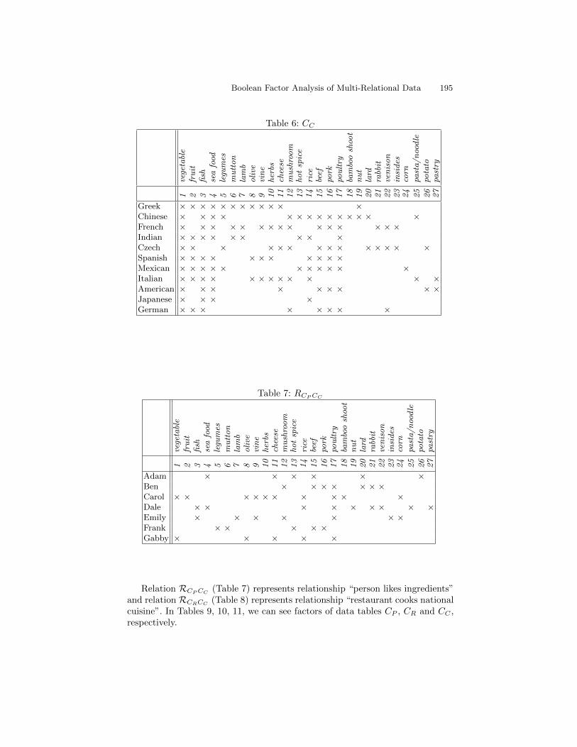
Table 6: CC

vege

tabl

efr

uit

fish

sea

food

legu

mes

mu

tto

nla

mb

oli

vevi

ne

her

bsch

eese

mu

shro

om

ho

tsp

ice

rice

beef

pork

pou

ltry

bam

boo

shoo

tn

ut

lard

rabb

itve

nis

on

insi

des

corn

past

a/

noo

dle

pota

topa

stry

1 2 3 4 5 6 7 8 9 10

11

12

13

14

15

16

17

18

19

20

21

22

23

24

25

26

27

Greek × × × × × × × × × × × ×Chinese × × × × × × × × × × × × × ×French × × × × × × × × × × × × × × ×Indian × × × × × × × × ×Czech × × × × × × × × × × × × × ×Spanish × × × × × × × × × × ×Mexican × × × × × × × × × × ×Italian × × × × × × × × × × × ×American × × × × × × × × ×Japanese × × × ×German × × × × × × × ×

Table 7: RCPCC

vege

tabl

efr

uit

fish

sea

food

legu

mes

mu

tto

nla

mb

oli

vevi

ne

her

bsch

eese

mu

shro

om

ho

tsp

ice

rice

beef

pork

pou

ltry

bam

boo

shoo

tn

ut

lard

rabb

itve

nis

on

insi

des

corn

past

a/

noo

dle

pota

topa

stry

1 2 3 4 5 6 7 8 9 10

11

12

13

14

15

16

17

18

19

20

21

22

23

24

25

26

27

Adam × × × × × ×Ben × × × × × × ×Carol × × × × × × × × × ×Dale × × × × × × × × ×Emily × × × × × × ×Frank × × × × ×Gabby × × × × ×

Relation RCPCC(Table 7) represents relationship “person likes ingredients”

and relation RCRCC(Table 8) represents relationship “restaurant cooks national

cuisine”. In Tables 9, 10, 11, we can see factors of data tables CP , CR and CC ,respectively.


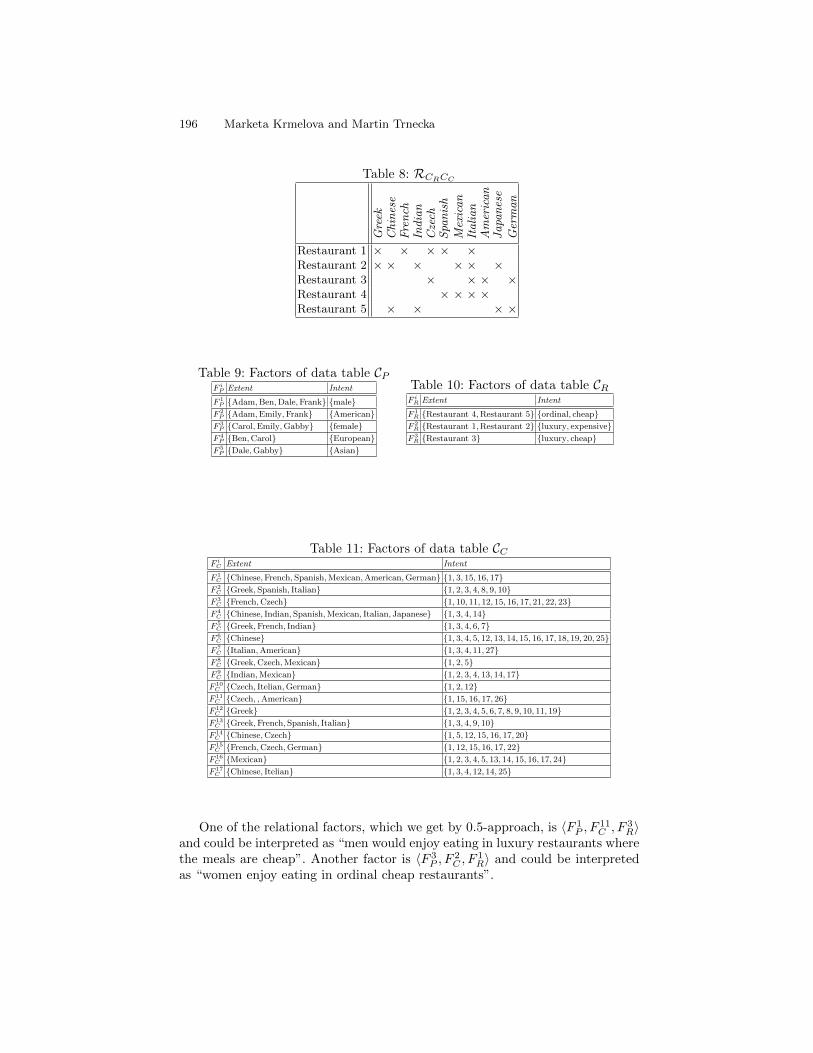
Table 8: RCRCC

Gre

ekC

hin

ese

Fre

nch

Ind

ian

Cze

chS

pan

ish

Mex

ica

nIt

ali

an

Am

eric

an

Ja

pan

ese

Ger

ma

n

Restaurant 1 × × × × ×Restaurant 2 × × × × × ×Restaurant 3 × × × ×Restaurant 4 × × × ×Restaurant 5 × × × ×

Table 9: Factors of data table CPF iP Extent Intent

F 1P {Adam,Ben,Dale,Frank} {male}

F 2P {Adam,Emily,Frank} {American}

F 3P {Carol,Emily,Gabby} {female}

F 4P {Ben,Carol} {European}

F 5P {Dale,Gabby} {Asian}

Table 10: Factors of data table CRF iR Extent Intent

F 1R {Restaurant 4,Restaurant 5} {ordinal, cheap}

F 2R {Restaurant 1,Restaurant 2} {luxury, expensive}

F 3R {Restaurant 3} {luxury, cheap}

Table 11: Factors of data table CCF iC Extent Intent

F 1C {Chinese,French, Spanish,Mexican,American,German} {1, 3, 15, 16, 17}

F 2C {Greek,Spanish, Italian} {1, 2, 3, 4, 8, 9, 10}

F 3C {French,Czech} {1, 10, 11, 12, 15, 16, 17, 21, 22, 23}

F 4C {Chinese, Indian,Spanish,Mexican, Italian, Japanese} {1, 3, 4, 14}

F 5C {Greek,French, Indian} {1, 3, 4, 6, 7}

F 6C {Chinese} {1, 3, 4, 5, 12, 13, 14, 15, 16, 17, 18, 19, 20, 25}

F 7C {Italian,American} {1, 3, 4, 11, 27}

F 8C {Greek,Czech,Mexican} {1, 2, 5}

F 9C {Indian,Mexican} {1, 2, 3, 4, 13, 14, 17}

F 10C {Czech, Itelian,German} {1, 2, 12}

F 11C {Czech, ,American} {1, 15, 16, 17, 26}

F 12C {Greek} {1, 2, 3, 4, 5, 6, 7, 8, 9, 10, 11, 19}

F 13C {Greek,French, Spanish, Italian} {1, 3, 4, 9, 10}

F 14C {Chinese,Czech} {1, 5, 12, 15, 16, 17, 20}

F 15C {French,Czech,German} {1, 12, 15, 16, 17, 22}

F 16C {Mexican} {1, 2, 3, 4, 5, 13, 14, 15, 16, 17, 24}

F 17C {Chinese, Itelian} {1, 3, 4, 12, 14, 25}

One of the relational factors, which we get by 0.5-approach, is 〈F 1P , F

11C , F 3

R〉and could be interpreted as “men would enjoy eating in luxury restaurants wherethe meals are cheap”. Another factor is 〈F 3

P , F2C , F

1R〉 and could be interpreted

as “women enjoy eating in ordinal cheap restaurants”.


4.2 Representation of connection between factors

We can represent the relational factors via graph (n-partite). See Figure 1, whichpresents the results from the previous example. Each group of nodes (F iP , F

iC , F

iR)

represents factors of a specific data table. Between two nodes, there is an edgeiff factors representing nodes satisfy the input relation. Relational factor is pathbetween nodes, which include at most one node from each group. For example,⟨F 2P , F

3C , F

1R

⟩is a relational factor because there is an edge between nodes F 2

P

and F 3C and between F 3

C and F 1R.

F1P

F2P

F3P

F4P

F5P

F1C

F2C

F3C

F4C

F5C

F6C

F7C

F8C

F9C

F10C

F11C

F12C

F13C

F14C

F15C

F16C

F17C

F1R

F2R

F3R

F1C

F2C

F3C

F4C

F5C

F6C

F7C

F8C

F9C

F10C

F11C

F12C

F13C

F14C

F15C

F16C

F17C

Fig. 1: Representation factors connections via graph.

5 Conclusion and Future Research

In this paper we present the new approach to BMF of multi-relational data, i.e.data which are composed from many data tables and relations between them.This approach, as opposed from to BMF, takes into account the relations anduses these relations to connect factors from individual data tables into one com-plex factor, which delivers more information than the simple factors.


A future research shall include the following topics: generalization multi-relational Boolean factorization for ordinal data, especially data over residuatedlattices. Design an effective algorithm for computing relational factors. Developnew approaches for connecting factors which utilize statistical methods and lastbut not least drive factor selection in the second data table, using informationabout factors in the first one and relation between them, for obtaining morerelevant data.

Acknowledgment We acknowledge support by the Operational Program Ed-ucation for Competitiveness Project No. CZ.1.07/2.3.00/20.0060 co-financed bythe European Social Fund and Czech Ministry of Education.

References

1. Bartholomew D. J., Knott M.: Latent Variable Models and Factor Analysis, 2ndEd., London, Arnold, 1999.

2. Belohlavek R., Vychodil V.: Discovery of optimal factors in binary data via a novelmethod of matrix decomposition. J. Comput. Syst. Sci. 76(1):3–20, 2010.

3. Ganter B., Wille R.: Formal Concept Analysis: Mathematical Foundations.Springer, Berlin, 1999.

4. Geerts F., Goethals B., Mielikainen T.: Tiling databases, Proc. Discovery Science2004, pp. 278–289.

5. Hacene M. R., Huchard M., Napoli A., Valtechev P.: Relational concept analy-sis: mining concept lattices from multi-relational data. Ann. Math. Artif. Intell.67(1)(2013), 81–108,.

6. Harman H. H.: Modern Factor Analysis, 2nd Ed. The Univ. Chicago Press,Chicago, 1970.

7. Huchard M., Napoli A., Rouane H. M., Valtchev P.: A proposal for combiningformal concept analysis and description logics for mining relational data. ICFCA2007.

8. Kim K.H.: Boolean Matrix Theory and Applications. Marcel Dekker, New York,1982.

9. Lippert, C., Weber, S. H., Huang, Y., Tresp, V., Schubert, M., and Kriegel, H.-P.: Relation-prediction in multi- relational domains using matrix-factorization. InNIPS 2008 Workshop on Structured Input - Structured Output, NIPS, 2008.

10. Lucchese C., Orlando S., Perego R.: Mining top-K patterns from binary datasetsin presence of noise, SIAM DM 2010, pp. 165–176.

11. Miettinen P.: On Finding Joint Subspace Boolean Matrix Factorizations. Proc.SIAM International Conference on Data Mining (SDM2012), pp. 954-965, 2012.

12. Miettinen P., Mielikainen T., Gionis A., Das G., Mannila H.: The discrete basisproblem, IEEE Trans. Knowledge and Data Eng. 20(10)(2008), 1348–1362.

13. Nau D.S., Markowsky G., Woodbury M.A., Amos D.B.: A mathematical analysisof human leukocyte antigen serology. Math Bioscience 40(1978), 243–270.

14. Vaidya J., Atluri V., Guo Q.: The role mining problem: finding a minimal descrip-tive set of roles. In: Proc. SACMAT 2007, pp. 175–184, 2007.

15. Xiang Y., Jin R., Fuhry D., Dragan F. F.: Summarizing transactional databaseswith overlapped hyperrectangles, Data Mining and Knowledge Discovery 23(2011),215–251.


Documents

Boolean Factor Analysis of Multi-Relational Data