Bondi-Sachs Formalism

Thomas Madler∗ and Jeffrey Winicour†‡

January 18, 2018

The Bondi-Sachs formalism of General Relativity is a metric-based treat-ment of the Einstein equations in which the coordinates are adapted to thenull geodesics of the spacetime. It provided the first convincing evidencethat that mass loss due to gravitational radiation is a nonlinear effect ofgeneral relativity and that the emission of gravitational waves from an iso-lated system is accompanied by a mass loss from the system. The asymptoticbehaviour of the Bondi-Sachs metric revealed the existence of the symmetrygroup at null infinity, the Bondi-Metzner-Sachs group, which turned out tobe larger than the Poincare group.

Contents

1 Introduction 2

2 The Bondi–Sachs metric 32.1 The electromagnetic analogue . . . . . . . . . . . . . . . . . . 5

3 Einstein equations and their Bondi-Sachs solution 8

4 The Bondi-Metzner-Sachs (BMS) group 17

5 The worldtube-null-cone formulation 21

6 Applications 23

∗Institute of Astronomy, University of Cambridge, Madingley Road, Cambridge, CB30HA, UK†Department of Physics and Astronomy University of Pittsburgh, Pittsburgh, PA

15260, USA‡Max-Planck-Institut fur Gravitationsphysik, Albert-Einstein-Institut, 14476 Golm,

Germany

1

arX

iv:1

609.

0173

1v3

[gr

-qc]

17

Jan

2018

1 Introduction

In a seminal 1960 Nature article (Bondi, 1960), Hermann Bondi presenteda new approach to the study gravitational waves in Einstein’s theory ofgeneral relativity. It was based upon the outgoing null rays along whichthe waves traveled. It was followed up in 1962 by a paper by Bondi, Met-zner and van der Burg (Bondi et al., 1962), in which the details were givenfor axisymmetric spacetimes. In his autobiography (Bondi, 1990, page 79),Bondi remarked about this work: “The 1962 paper I regard as the bestscientific work I have ever done, which is later in life than mathematicianssupposedly peak”. Soon after, Rainer Sachs (Sachs, 1962b) generalized thisformalism to non-axisymmetric spacetimes and sorted out the asymptoticsymmetries in the approach to infinity along the outgoing null hypersurfaces.The beautiful simplicity of the Bondi-Sachs formalism was that it only in-volved 6 metric quantities to describe a general spacetime. At this time, anindependent attack on Einstein’s equations based upon null hypersurfaceswas underway by Ted Newman and Roger Penrose (Newman and Penrose,1962, 2009). Whereas the fundamental quantity in the Bondi–Sachs for-malism was the metric, the Newman-Penrose approach was based upon anull tetrad and its curvature components. Although the Newman-Penroseformalism involved many more variables it led to a more geometric treat-ment of gravitational radiation, which culminated in Penrose’s (Penrose,1963) description in terms of the conformal compactification of future nullinfinity, denoted by I+ (pronounced “scri plus” for script I plus). It wasclear that there were parallel results emerging from these two approachesbut the two formalisms and notations were completely foreign. At meetings,Bondi would inquire of colleagues, including one of us (JW), “Are you youa qualified translator?”. This article describes the Bondi-Sachs formalismand how it has evolved into a useful and important approach to the currentunderstanding of gravitational waves.

Before 1960, it was known that linear perturbations hab of the Minkowskimetric ηab = diag(−1, 1, 1, 1) obeyed the wave equation (in geometric unitswith c = 1) (

− ∂2

∂t2+ δij

∂2

∂yi∂yj

)hab = 0 , (1)

where the standard Cartesian coordinates yi = (y1, y2, y3) satisfy the har-monic coordinate condition to linear order. It was also known that theselinear perturbations had coordinate (gauge) freedom which raised seriousdoubts about the physical properties of gravitational waves. The retarded

2

time u and advanced time v,

u = t− r , v = t+ r , r2 = δijyiyj , (2)

characteristic hypersurfaces of the hyperbolic equations (1), i.e. hypersur-faces along which wavefronts can travel.

These characteristic hypersurfaces are also null hypersurfaces, i.e. theirnormals, ka = −∇au and na = −∇av are null, ηabkakb = ηabnanb = 0.Note that it is a peculiar property of null hypersurfaces that their normaldirection is also tangent to the hypersurface, i.e. ka = ηabkb is tangent tothe u = const hypersurfaces. The curves tangent to ka are null geodesics,called null rays, and generate the u = const outgoing null hypersurfaces.Bondi’s ingenuity was to use such a family of outgoing null rays forming thesenull hypersurfaces to build spacetime coordinates for describing outgoinggravitational waves.

An analogous formalism based upon ingoing null hypersurfaces is alsopossible and finds applications in cosmology (Ellis et al., 1985) but is ofless physical importance in the study of outgoing gravitational waves. Thenew characteristic approach to gravitational phenomenon complemented thecontemporary 3+1 treatment being developed by Arnowitt et al. (1961).

2 The Bondi–Sachs metric

The Bondi-Sachs coordinates xa = (u, r, xA) are based on a family of out-going null hypersurfaces u = const The hypersurfaces x0 = u = const arenull, i.e. the normal co-vector ka = −∂au satisfies gab(∂au)(∂bu) = 0, sothat guu = 0, and the corresponding future pointing vector ka = −gab∂bu istangent to the null rays. Two angular coordinates xA, (A,B,C, ... = 2, 3),are constant along the null rays, i.e. ka∂ax

A = −gab(∂au)∂bxA = 0, so

that guA = 0. The coordinate x1 = r, which varies along the null rays, ischosen to be an areal coordinate such that det[gAB] = r4q, where q(xA) isthe determinant of the unit sphere metric qAB associated with the angularcoordinates xA, e.g. qAB = diag(1, sin2 θ) for standard spherical coordinatesxA = (θ, φ). The contravariant components gab and covariant componentsgab are related by gacgcb = δab , which in particular implies grr = 0 (fromδur = 0) and grA = 0 (from δuA = 0).

In the resulting xa = (u, r, xA) coordinates, the metric takes the Bondi-Sachs form,

gabdxadxb = −V

re2βdu2− 2e2βdudr+ r2hAB

(dxA−UAdu

)(dxB −UBdu

),

(3)

3

wheregAB = r2hAB with det[hAB] = q(xA), (4)

so that the conformal 2-metric hAB has only two degrees of freedom.The determinant condition implies hAB∂rhAB = hAB∂uhAB = 0, where

hAChCB = δAB. Hereafter DA denotes the covariant derivative of the met-ric hAB, with DA = hABDB. The corresponding non-zero contravariantcomponents of the metric (3) are

gur = −e−2β , grr =V

re−2β , grA = −UAe−2β , gAB =

1

r2hAB .

(5)A suitable representation of hAB with two functions γ(u, r, θ, φ) and

δ(u, r, θ, φ) corresponding to the + and × polarization of gravitational wavesis (van der Burg, 1966; Winicour, 2013)

hABdxAdxB =

(e2γdθ2 + e−2γ sin2 θdφ2

)cosh(2δ) + 2 sin θ sinh(2δ)dθdφ .

(6)This differs from the original form of Sachs (Sachs, 1962b) by the transforma-tion γ → (γ + δ)/2 and δ → (γ−δ)/2, which gives a less natural descriptionof gravitational waves in the weak field approximation. In the original ax-isymmetric Bondi metric (Bondi et al., 1962) with rotational symmetry inthe φ-direction, δ = Uφ = 0 and γ = γ(u, r, θ), resulting in the metric

g(B)ab dx

adxb =(− V

re2β + r2Ue2γ

)du2 − 2e2βdudr − r2Ue2γdudθ

+r2(e2γdθ2 + e−2γ sin2 θdφ2

), (7)

where U ≡ U θ. Note that the original Bondi metric also has the reflectionsymmetry φ→ −φ so that it is not suitable for describing an axisymmetricrotating star.

In Bondi’s original work, the areal coordinate r was called a luminositydistance but this terminology is misleading because of its different meaningin cosmology (Jordan et al., 1960, see Sec. 3.3). The areal coordinate rbecomes singular when the expansion Θ of the null hypersurface vanishes,where (Sachs, 1961, 1962b)

Θ = ∇a(e−2βka) =2

re−2β , ka∂a = −gur∂r. (8)

In contrast, the standard radial coordinate along the null rays in the Newman-Penrose formalism (Newman and Penrose, 1962, 2009) is the affine param-eter λ, which remains regular when Θ = 0. The areal distance and affine

4

parameter are related by ∂rλ = e2β. Thus the areal coordinate remainsnon-singular provided β remains finite. For a version of the Bondi-Sachsformalism based upon an affine parameter, see (Winicour, 2013).

2.1 The electromagnetic analogue

The electromagnetic field in Minkowski space with its two degrees of freedompropagating along null hypersurfaces provides a simple model to demon-strate the essential features and advantages of the Bondi–Sachs formal-ism (Tamburino and Winicour, 1966). Consider the Minkowski metric inoutgoing null spherical coordinates (u, r, xA) corresponding to the flat spaceversion of the Bondi-Sachs metric,

ηabdxadxb = −du2 − 2drdu+ r2qABdx

AdxB . (9)

Assume that the charge-current sources of the electromagnetic field areenclosed by a 3-dimensional timelike worldtube Γ, with spherical cross-sections of radius r = R, such that the outgoing null cones Nu from thevertices r = 0 (Fig. 1) intersect Γ at proper time u in spacelike spheres Su,which are coordinatized by xA.

The electromagnetic field Fab is represented by a vector potential Aa,Fab = ∇aAb −∇bAa, which has the gauge freedom

Aa → Aa +∇aχ . (10)

Choosing the gauge transformation

χ(u, r, xA) = −∫ r

RArdr

′ (11)

leads to the null gauge Ar = 0, which is the analogue of the Bondi-Sachscoordinate condition grr = grA = 0. The remaining gauge freedom χ(u, xA)may be used to set either

Au|Γ = Au(u,R, xA) = 0 or limr→∞

Au(u, r, xA) = 0. (12)

Hereafter, we implicity assume that the limit r → ∞ is taken holding u =const and xA = const. There remains the freedom AB → AB +∇B χ(xC).

The vacuum Maxwell equations M b := ∇aF ab = 0 imply the identity

0 ≡ ∇bM b = ∂uMu +

1

r2∂r(r

2M r) +1√q∂C(√qMC). (13)

5

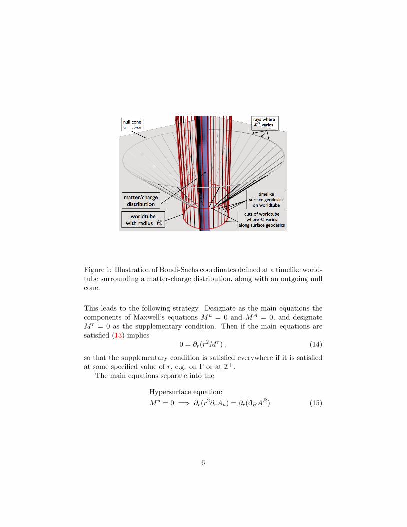
Figure 1: Illustration of Bondi-Sachs coordinates defined at a timelike world-tube surrounding a matter-charge distribution, along with an outgoing nullcone.

This leads to the following strategy. Designate as the main equations thecomponents of Maxwell’s equations Mu = 0 and MA = 0, and designateM r = 0 as the supplementary condition. Then if the main equations aresatisfied (13) implies

0 = ∂r(r2M r) , (14)

so that the supplementary condition is satisfied everywhere if it is satisfiedat some specified value of r, e.g. on Γ or at I+.

The main equations separate into the

Hypersurface equation:

Mu = 0 =⇒ ∂r(r2∂rAu) = ∂r(ðBAB) (15)

6

and the

Evolution equation:

MA = 0 =⇒ ∂r∂uAB =1

2∂2rAB −

r2

2ðC(ðBAC − ðCAB) +

1

2∂rðBAu,

(16)

where hereafter ðA denotes the covariant derivative with respect to the unitsphere metric qAB, with ðA = qABðB. The supplementary condition M r = 0takes the explicit form

∂u(r2∂rAu) = ðB(∂rAB − ∂uAB + ðBAu). (17)

A formal integration of the hypersurface equation yields

∂rAu =Q(u, xA) + ðBAB

r2+O(1/r3) , (18)

where Q(u, xA) enters as a function of integration. In the null gauge withAr = 0, the radial component of the electric field corresponds to Er =Fru = ∂rAu. Thus, using the divergence theorem to eliminate ðBAB, thetotal charge enclosed in a large sphere is

q(u) := limr→∞

1

4π

∮Err

2 sin θdθdφ =1

4π

∮Q(u, xA) sin θdθdφ, (19)

where∮

indicates integration over the 2-sphere. This motivates callingQ(u, xA) the charge aspect. The integral of the supplementary condition(17) over a large sphere then gives the charge conservation law

dq(u)

du= 0. (20)

The main equations (15) and (16) give rise to a hierarchical integrationscheme given the following combination of initial data on the initial nullcone Nu0 , initial boundary data on the cross-section Su0 of Γ and boundarydata on Γ:

AB∣∣Nu0

, ∂rAu∣∣Su0

, ∂uAB∣∣Γ. (21)

Then, in sequential order, (15) is an ordinary differential equation alongthe null rays which determines Au and (16) is an ordinary differential equa-tion which determines ∂uAB. Together with the supplementary equation(17), they give rise to the following evolution algorithm:

7

1. In accord with (12), choose a gauge such that Au∣∣Γ

= 0.

2. Given the initial data AB∣∣Nu0

and ∂rAu∣∣Su0

, the hypersurface equation

(15) can be integrated along the null rays of Nu0 to determine Au onthe initial null cone Nu0 .

3. Given the initial boundary data ∂uAB|Su0, the radial integration of

the evolution equation (16) determines ∂uAB on the initial null coneNu0 .

4. (a) From ∂uAB|Nu0, AB can be obtained in a finite difference approx-

imation on the null cone u = u0 + ∆u.

(b) From knowledge of AB|Nu0and Au|Nu0

, the the supplementary

condition (17) determines ∂u∂rAu∣∣Su0

so that ∂rAu|Su0+∆ucan

also be obtained in a finite difference approximation.

5. This procedure can be iterated to determined a finite difference ap-proximation for AB and Au on the null cone u = u0 + n∆u.

An analogous algorithm for solving the Bondi-Sachs equations has beenimplemented as a convergent evolution code (see Sec. 5).

3 Einstein equations and their Bondi-Sachs solu-tion

The Einstein equations, in geometric units G = c = 1, are

Eab := Rab −1

2gabR

cc − 8πTab = 0 , (22)

where Rab is the Ricci tensor, Rcc its trace and Tab the matter stress-energytensor. Before expressing the Einstein equations in terms of the Bondi-Sachsmetric variables (3), consider the consequence of the contracted Bianchiidentities. Assuming the matter satisfies the divergence-free (C5) condition∇bT ba = 0, the Bianchi identities imply

0 = ∇bEba =1√−g

∂b

(√−gEba

)+

1

2(∂ag

bc)Ebc . (23)

In analogy to the electromagnetic case, this leads to the designation ofthe components of Einstein’s equations, consisting of

Eua = 0 , EAB −1

2gABg

CDECD = 0 , (24)

8

as the main equations. Then if the main equations are satisfied, referring tothe metric (3), Ebr = −e2βEub = −e2βgbaEua = 0 and the a = r component ofthe conservation condition (23) reduces to (∂rg

AB)EAB = −(2/r)gABEAB =0 so that the component gABEAB = 0 is trivially satisfied. Here we assumethat the areal coordinate r is non-singular.

The retarded time u and angular components xA of the conservationcondition (23) now reduce to

∂r(r2e2βEru) = 0 , ∂r(r

2e2βErA) = 0 (25)

so that the Eru and ErA equations are satisfied everywhere if they are satisfiedon a finite worldtube Γ or in the limit r → ∞. Furthermore, if the nullfoliation consists of non-singular null cones, they are automatically satisfieddue to regularity conditions at the vertex r = 0. These equations were calledsupplementary conditions by Bondi and Sachs. Evaluated in the limit r →∞ they are related to the asymptotic flux conservation laws for total energyand angular momentum. In particular, the equation limr→∞(r2Eru) = 0gives rise to the famous Bondi mass loss equation (see (61)).

The main Einstein equations separate further into the

Hypersurface equations: Eua = 0 (26)

and the

Evolution equations: EAB −1

2gABg

CDECD = 0. (27)

In terms of the metric variables (3) the hypersurface equations consistof one first order radial differential equation determining β along the nullrays,

Eur = 0 ⇒ ∂rβ =r

16hAChBD(∂rhAB)(∂rhCD) + 2πrTrr , (28)

two second order radial differential equations determining UA,

EuA = 0 ⇒ ∂r

[r4e−2βhAB(∂rU

B)

]= 2r4∂r

( 1

r2DAβ

)−r2hEFDE(∂rhAF ) + 16πr2TrA , (29)

and a radial equation to determine V ,

Euu = 0 ⇒ 2e−2β(∂rV ) = R − 2hAB[DADBβ + (DAβ)(DBβ)

]+e−2β

r2DA

[∂r(r

4UA)]− 1

2r4e−4βhAB(∂rU

A)(∂rUB)

+8π[hABTAB − r2T aa

], (30)

9

where DA is the covariant derivative and R is the Ricci scalar with respectto the conformal 2-metric hAB.

The evolution equations can be picked out by introducing a complexpolarization dyad ma satisfying ma∇au = 0 which is tangent to the nullhypersurfaces and points in the angular direction with components ma =(0, 0,mA). Imposing the normalization hAB = 1

χχ(mAmB + mBmA), with

χ ∈ C, mAmA = χχ, mA = hABm

B, and mAmA = 0 determines mA

up to the phase freedom mA → eiηmA, which can be fixed by convention.Note, the Newman-Penrose convention for the normalisation of mA usesχχ = 1 Newman and Penrose (2009) while numerical applications of theBondi-Sachs formalism use χχ = 2 (Winicour, 2012). The latter has theadvantage to avoid factors containing

√2 in the components of the tetrad

which are non-practical in numerical work. Further note that the definitionof the dyad ma here relates to the null vector ma of the Newman-Penroseformalism Newman and Penrose (2009) as ma

(NP ) = r−1ma, because ma(NP )

is defined with respect to gab rather that hAB. The symmetric 2-tensor EABcan then be expanded as

EAB =1

(χχ)2(ECDm

CmD)mAmB+1

(χχ)2(ECDm

CmD)mAmB+1

2hABh

CDECD,

(31)where we have shown that hCDECD = 0 is trivially satisfied. Consequently,the evolution equations reduce to the complex equation mAmBEAB = 0,which takes the form (Winicour, 1983, 2012)

mAmB

r∂r[r(∂uhAB)]− 1

2∂r[rV (∂rhAB)]− 2eβDADBe

β

+ hCADB[∂r(r2UC)]− 1

2r4e−2βhAChBD(∂rU

C)(∂rUD)

+r2

2(∂rhAB)(DCU

C) + r2UCDC(∂rhAB)

− r2(∂rhAC)hBE(DCUE −DEUC)− 8πe2βTAB

= 0. (32)

It comprises a radial equation which determines the retarded time derivativeof the two degrees of freedom in the conformal 2-metric hAB.

As in the electromagnetic case, the main equations can be radially inte-grated in sequential order. In order to illustrate the hierarchical integrationscheme we follow Bondi and Sachs by considering an asymptotic 1/r ex-pansion of the solutions in an asymptotic inertial frame, with the mattersources confined to a compact region. This ansatz of a 1/r-expansion of the

10

metric leads to the peeling property of the Weyl tensor in the spin-coefficientapproach (see (Newman and Penrose, 2009)). For a more general approachin which logarithmic terms enter the far field expansion and only a partialpeeling property results, see (Winicour, 1985).

In the asymptotic inertial frame, often referred to as a Bondi frame, themetric approaches the Minkowski metric (9) at null infinity, so that

limr→∞

β = limr→∞

UA = 0 , limr→∞

V

r= 1 , lim

r→∞hAB = qAB . (33)

Later, in Sec. 4, we will justify these asymptotic conditions in terms of aPenrose compactification of I+.

For the purpose of integrating the main equations, we prescribe the fol-lowing data:

1. The conformal 2-metric hAB on an initial null hypersurface N0, u = u0,which has the asymptotic 1/r expansion

hAB(u0, r, xC) = qAB +

cAB(u0, xE)

r+dAB(u0, x

E)

r2+ ..., (34)

where the condition hAChCB = δAB implies

hAB = qAB − cAB

r− dAB − qACcBDcCD

r2+ ... (35)

with cAB := qADqBEcDE and dAB := qADqBEdDE . Furthermore, thederivative of the determinant condition det(hAB) = q(xC) requires

qABcAB = 0 , qABdAB =1

2cABcAB , qAB∂ucAB = 0 ,

qAB∂udAB − cAB∂ucAB = 0. (36)

2. The 1/r coefficient of the conformal 2-metric hAB for retarded timesu ∈ [u0, u1], u1 > u0,

cAB(u, xC) := limr→∞

r(hAB − qAB) , (37)

which describes the time dependence of the gravitational radiation.

3. A function M(u, xA) at the initial time u0,

M(u0, xA) := −1

2limr→∞

[V (u0, r, xC)− r] , (38)

which is called the mass aspect.

11

4. A co-vector field LA(u0, xC) on the sphere at the initial time u0,

LA(u0, xC) := −1

6limr→∞

(r4e−2βhAB∂rU

B − rðBcAB), (39)

which is the angular momentum aspect.

In terms of a complex dyad qA = limr→∞mA on the unit sphere so that

qAB = 1χ2 (qAqB + qB qA), e.g. for the choice qA = χ√

2(1, i/ sin θ), the real

and imaginary part of

σ0 =1

2χ2qAqBcAB =

1

2

(cθθ −

cφφ

sin2 θ

)+ i

(cθφ

sin θ

)(40)

correspond, respectively, to the + and × polarization modes of the strainmeasured by a gravitational wave detector at large distance from the source(Thorne, 1983). Traditionally, the radiative strain σ0 has also been calledthe shear because it measures the asymptotic shear of the outgoing nullhypersurfaces in the sense of geometric optics,

σ0 = limr→∞

(1

χ2r2qAqB∇A∇Bu

). (41)

Note that σ0 corresponds to the leading order of the spin coefficient σ of theNewman-Penrose formalism (Newman and Penrose, 2009). The retardedtime derivative

NAB =1

2∂ucAB(u, xC), (42)

called the news tensor, determines the energy flux of gravitational radia-tion. The factor of 1/2 in (42) is introduced to recover the Bondi’s originaldefinition of the news in the axisymmetric case. The news tensor is a ge-ometrically determined tensor field independent of the choice of u-foliation(see the discussion concerning (73)).

Relative to a choice of polarization dyad, the Bondi news function is

N =1

χ2qAqBNAB , (43)

in particular the news function is the retarded time derivative of the radia-tion strain N = ∂uσ0.

Note, in carrying out the 1/r expansion of the field equations the co-variant derivative DA corresponding to the metric hAB is related to thecovariant derivative ðA corresponding to the unit sphere metric qAB by

DAVB = ðAV B + CBAEV E , (44)

12

where

CBAE =1

2rqBF (ðA cFE + ðE cFA − ðF cAE) +O(1/r2). (45)

Given the asymptotic gauge conditions (33) and the initial data (35),(38), (39), (37) on N0, the formal integration of the main equations at larger proceeds in the following sequential order:

1. Integration of the β-hypersurface equation gives

β(u0, r, xA) = − 1

32

cABcABr2

+O(r−3) . (46)

2. Insertion of the data (34) and the solution for β into the UA hyper-surface equation (29) yields

∂r

[r4e−2βhAB(∂rU

B)

]= ðEcAE +

SA(u0, xC)

r+O(1/r2) (47)

whereSA(u0, x

C) = ðB(2dAB − qFGcBGcAF ). (48)

As a result, unless SA = 0, integration of (47) leads to a logarithmicr−4 ln r term in ∂rU

A, which is ruled out by the assumption of anasymptotic 1/r expansion. This leads to the following result. Becauseof the determinant condition (36),

qAqBqFGcBGcAF =1

2qAqB(qF qG + qF qG)cBGcAF = 0

so that

qFGcBGcAF =1

2qABc

FGcFG.

As a result

SA = ðB(2dAB −1

2qAB c

FGcFG),

or, again using (36), the logarithmic condition becomes

SA = 2ðBbAB = 0 (49)

where bAB = dAB − 12qABq

CDdCD is symmetric and trace-free. It nowfollows readily from the powerful Newman-Penrose ð-calculus (New-man and Penrose, 1962, 2009) that the condition SA = 0 implies

13

bAB = 0. In order to obtain this result without ð-calculus, first useqABbAB = 0 to obtain

SA = 2qBEðEbAB = 2qBE(ðEbAB − ðAbEB)

so that (49) also implies

εEAðEbAB = 0, (50)

where εAB = iχχ(qAqB−qAqB) is the antisymmetric surface area tensor

on the unit sphere. Consider the component ΦBεEAðEbAB = 0, whereΦB is a Killing vector on the unit sphere. Then

0 = ΦBεEAðEbAB = εEAðE(bABΦB)− εEAbABqECðCΦB. (51)

But, as a result of Killing’s equation ðAΦB +ðBΦA = 0 and the trace-free property of bAB,

εEAbAB qECðCΦB = εEAbAB qEC

[1

2(ðCΦB + ðBΦC) +

1

2(ðCΦB − ðBΦC)

]=

1

2εEAbAB qECε

CBεFGðFΦG (52)

=1

2qABbAB εFGðFΦG (53)

= 0, (54)

where we have used the identity TAB = 12εABε

CDTCD satisfied in 2-dimensions by an arbitrary antisymmetric tensor TAB. Consequently,(51) gives εEAðE(bABΦB) = 0 so that bABΦB = ðAb for some scalar b.Inserting this result into (49) yields SAΦA = 2ðAðAb = 0 whose onlysolution is b = const. Consequently, bABΦB = 0 which is sufficientto show the desired result that the two independent components ofbAB vanish. Thus dAB consists purely of a trace term dictated by thedeterminant condition (36).

Hence, applying this constraint and integrating (47) once yields

r4e−2βhAB∂rUB = −6LA(u0, x

B) + r(ðBcAB

)+O(r−1) . (55)

3. Rearranging (55) while using (35) and (46) and subsequent radial in-tegration of ∂rU

A with the asypmtotic data (39) gives

UA(u0, r, xB) = −ðBcAB

2r2+

1

r3

(2LA +

1

3cAEðF cEF

)+O(r−4). (56)

14

Note (56) corrects the non-linear coefficients in the O(r−3) terms ofBondi and Sachs’ original works and agrees with the correspondingcoefficient of Barnich and Troessaert (2010a) up to the redefinitionLA → −3LA.

4. With the initial data (34) and initial values of β and UA, the V -hypersurface equation (30) can be integrated to find the asymptoticsolution

V (u0, r, xA) = r − 2M(u0, x

A) +O(r−1) . (57)

Here M(u, xA) is called the mass aspect since in the static, spheri-cally symmetric case, where hAB = qAB, β = UA = 0 and M(u, xA) =m, the metric (3) reduces to the Eddington-Finkelstein metric for aSchwarzschild mass m.

5. Insertion of the solutions for β, UA and V into the evolution equation(32) yields to leading order that qAqB∂udAB = 0, consistent with thedeterminant condition (36).

6. With the asymptotic solution of the metric, the leading order coeffi-cient of the Eru supplementary equation gives

2∂uM = ðAðBNAB −NABNAB . (58)

Since NAB is assumed known for u0 ≤ u ≤ u1, integration determinesthe mass aspect M in terms of its initial value M(u0, x

A).

7. The leading order coefficient of the ErA supplementary equation deter-mines the time evolution of the angular momentum aspect LA,

−3∂uLA = ðAM −1

4ðE(ðEðF cAF − ðAðF cEF ) +

1

8ðA(cEFN

EF )

−ðC(cCFNFA

)+

1

2cEF (ðANEF ) (59)

The motivation for calling LA(u, xA) the angular momentum aspectcan be seen in the non-vacuum case where its controlling ErA supple-mentary equation is coupled to the angular momentum flux r2T rA of thematter field to null infinity. Together with (58), (59) shows that thetime evolution of LA is entirely determined by NAB for u0 ≤ u ≤ u1

and the initial values of LA, M and cAB at u = u0.

15

This hierarchical integration procedure shows how the boundary con-ditions (33) and data (35), (38), (39), (37) uniquely determine a formalsolution of the field equation in terms of the coefficients of an asymptotic1/r expansion. In particular, the supplementary equations determine thetime derivatives of M and LA, whereas the hypersurface equations deter-mine the higher order expansion coefficients. However, this formal solutioncannot be cast as a well-posed evolution problem to determine the metric foru > u0 because the necessary data, e.g. cAB(u, xC), lies in the future of theinitial hypersurface at u0. Nevertheless, this formal solution led Bondi tothe first clear understanding of mass loss due to gravitational radiation. Itgives rise to the interpretation of the supplementary conditions as flux con-servation laws for energy-momentum and angular momentum (Tamburinoand Winicour, 1966; Goldberg, 1974).

The time-dependent Bondi mass m(u) for an isolated system is

m(u) :=1

4π

∮M(u, θ, φ) sin θdθdφ . (60)

The integration of (58) over the sphere, using the definition of the newsfunction (43), gives the famous Bondi mass loss formula

d

dum(u) = − 1

4π

∮|N |2 sin θdθdφ , (61)

where the first term of (58) integrates out because of the divergence theo-rem. The positivity of the integrand in (61) shows that if a system emitsgravitational waves, i.e. if there is news, then its Bondi mass must decrease.If there is no news, i.e. N = 0, the Bondi mass is constant. The expressionsfor the Bondi mass (56) and the mass loss formula (57) were generalized forspacetimes with non-zero cosmological constant by Saw, (2016) and higher-dimensional generalisations of (56) and (57) can be found in Tanabe et al.(2011) and Godazgar and Reall (2012)

Here (59) corrects the original equations Bondi and Sachs for the timeevolution of the angular momentum aspect LA. For the Bondi metric inwhich γ(u, r, θ) = c(u, θ)/r +O(1/r3), (59) becomes

− 3∂uLθ = ∂θM +1

2c(∂θN)− 3

2N(∂θc) , (62)

here N = ∂uc is the axisymmetric Bondi news function. The asymptoticapproach of Bondi and Sachs illustrates the key features of the metric basednull cone formulation of general relativity. Nevertheless, assigning bound-ary data such as the news function N at large distances is non-physical as

16

opposed to determining N by evolving an interior system (see Sec. 5). Inparticular, assignment of boundary data on a finite worldtube surroundingthe source leads to gauge conditions in which the asymptotic Minkowskibehavior (33) does not hold.

4 The Bondi-Metzner-Sachs (BMS) group

The asymptotic symmetries of the metric can be most clearly and elegantlydescribed using a Penrose compactification of null infinity (Penrose, 1963).In that case the assumption of an asymptotic series expansion in 1/r becomesa smoothness condition at I+.

In Penrose’s compactification of null infinity, I+ is the finite boundary ofan unphysical space time containing the limiting end points of null geodesicsin the physical space time. If gab is the metric of the physical space timeand gab denotes the unphysical spacetime the two metrics are conformallyrelated via gab = Ω2gab, where gab is smooth (at least C3) and Ω = 0 atI+. Asymptotic flatness requires that I+ has the topology R× S2 and that∇aΩ vanishes nowhere at I+. The conformal space and physical space Riccitensors are related by

Ω2Rab = Ω2Rab + 2Ω∇a∇bΩ + gab

[Ω∇c∇cΩ− 3(∇cΩ)∇cΩ

](63)

where ∇a is the covariant derivative with respect to gab. Separating out thetrace of (63), evaluation of the physical space vacuum Einstein equationsRab = 0 at I+ implies

0 = [(∇cΩ)∇cΩ]I+ (64a)

0 =[∇a∇bΩ−

1

4gab∇c∇cΩ

]I+

. (64b)

The first condition shows that I+ is a null hypersurface and the secondassures the existence of a conformal transformation Ω−2gab = Ω−2gab suchthat ∇a∇bΩ|I+ = 0. Thus there is a set of preferred conformal factors Ωfor which null infinity is a divergence-free (∇c∇cΩ|I+ = 0) and shear-free(∇a∇bΩ|I+ = 0) null hypersurface.

A coordinate representation xa = (u, `, xA) of the compactified spacecan be associated with the Bondi–Sachs physical space coordinates in Sec. 2by the transformation xa = (u, `, xA) = (u, 1/r, xA). Here the inverse arealcoordinate ` = 1/r also serves as a convenient choice of conformal factor

17

Ω = `. This gives rise to the conformal metric

gabdxadxb = `3V e2βdu2 + 2e2βdud`+ hAB

(dxA − UAdu

)(dxB − UBdu

),

(65)where det(hAB) = q. The leading coefficients of the conformal space metricare subject to the Einstein equations (63) according to

hAB = HAB(u, xC) + `cAB(u, xc) +O(`2) (66)

β = H(u, xC) +O(`2) (67)

UA = HA(u, xC) + 2`e2HHABDBH +O(`2) (68)

`2V = DAHA + `

[1

2R+DADAe

2H]

+O(`2), (69)

where hereR is the Ricci scalar and DA is the covariant derivative associatedwith HAB.

In (65), H, HA and HAB have a general form which does not correspondto an asymptotic inertial frame. In order to introduce inertial coordinatesconsider the null vector na = gab∇b` which is tangent to the null geodesicsgenerating I+. In a general coordinate system, it has components at I+

na|I+ =(e−2H , 0,−e−2HHA

)(70)

arising from the contravariant metric components

gab∣∣∣I+

=

0 e−2H 0e−2H 0 −HAe−2H

0 −HAe−2H HAB

. (71)

Introduction of the inertial version of angular coordinates by requiring

na∂axA|I+ = 0

results in HA = 0. Next, introduction of the inertial version of a retardedtime coordinate by requiring that u be an affine parameter along the gener-ators of I+, with

na∂au∣∣∣I+

= 1,

results in H = 0. It also follows that ` is a preferred conformal factorso that the divergence free and shear free condition ∇a∇b`I+ = 0 impliesthat ∂uHAB = 0. This allows a time independent conformal transformation` → ω(xC)` such that HAB → qAB, so that the cross-sections of I+ have

18

unit sphere geometry. In this process, the condition H = 0 can be retainedby an affine change in u.

Thus it is possible to establish an inertial coordinate system xa at I+,which justifies the Bondi-Sachs boundary conditions (33). In these inertialcoordinates, the conformal metric has the asymptotic behavior

hAB = qAB(u, xC) + `cAB(u, xC) +O(`2) (72a)

β = O(`2) (72b)

UA = −ðBcAB2`2

+2LA`3 +O(`4) (72c)

`3V = `2 − 2M`3 +O(`4), (72d)

showing that the Bondi-Sachs variables cAB, mass aspect M and angularmomentum aspect LA are the the leading order coefficients of a Taylor seriesat null infinity with respect to the preferred conformal factor `.

It follows from (64b) that `−1∇a∇b` has a finite limit at I+. In inertialcoordinates the tensor field

Nab = ζ∗(

lim`→0

`−1∇a∇b`), (73)

where ζ∗ represents the pull-back to I+ (Geroch, 1977), i.e. the intrinsic(u, xA) components, equals the news tensor (73). It also follows that Nab isindependent of the choice of conformal factor Ω = ` → ω`, ω > 0. This es-tablishes the important result that the news tensor is a geometrically definedtensor field on I+ independent of the choice of u-foliation.

The BMS group is the asymptotic isometry group of the Bondi-Sachsmetric (3). In terms of the physical space metric, the infinitesimal generatorsξa of the BMS group satisfy the asymptotic version of Killing’s equation

Ω2Lξgab|I+ = −2Ω2∇(aξb)|I+ = 0 , (74)

where Lξ denotes the Lie derivative along ξa. In terms of the conformalspace metric (72) with conformal factor Ω = `, this implies[

∇(aξb) − `−1gabξc∂c`]`=0

= 0. (75)

This immediately requires ξc∂c` = 0, i.e. the generator is tangent to I+ and`−1ξc∂c`|I+ = ∂`ξ

`|I+ . Then (75) takes the explicit form[gac∂cξ

b + gbc∂cξa − ξc∂cgab − gab∂`ξ`

]I+

= 0 , (76)

19

where (71) reduces in the inertial frame to

gab∣∣∣I+

=

0 1 01 0 00 0 qAB

. (77)

Since only gab|I+ enters (76), it is simple to analyze. This leads to thegeneral solution

ξa∂a|`=0 =[α(xC) +

u

2ðBfB(xC)

]∂u + fA(xC)∂A (78)

where fA(xC) is a conformal killing vector of the unit sphere metric,

ð(AfB) − 1

2qABðCfC = 0 . (79)

These constitute the generators of the BMS group.The BMS symmetries with fA = 0 are called supertranslations; and

those with α = 0 describe conformal transformations of the unit sphere,which are isomorphic to the orthochronous Lorentz transformations (Sachs,1962a). The supertranslations form an infinite dimensional invariant sub-group of the BMS group. Of special importance, the supertranslations con-sisting of l = 0 and l = 1 spherical harmonics, e.g. α = a + ax sin θ cosφ +ay sin θ sinφ + az cos θ, form an invariant 4-dimensional translation groupconsisting of time translations (a) and spatial translations (ax, ay, az). Thisallows an unambiguous definition of energy-momentum. However, becausethe Lorentz group is not an invariant subgroup of the BMS group therearises a supertranslation ambiguity in the definition of angular momentum.Only in special cases, such as stationary spacetimes, can a preferred Poincaregroup be singled out from the BMS group.

Consider the finite supertranslation, u = u + α(xA) + O(`), with xA =xA, where the O(`) term is required to maintain u as a null coordinate.Under this supertranslation, the radiation strain or asymptotic shear (41),

i.e. σ(u, xC) = r2

χ2 qAqB∇A∇Bu|I+ , transforms according to

σ(u, xC) =r2

χ2qAqB∇A∇Bu|I+ = σ(u, xC) +

1

χ2qAqBðAðBα(xC). (80)

This reveals the gauge freedom in the radiation stain under supertransla-tions. Note, because α is a real function, in the terminology of the Newman-Penrose spin-weight formalism (Newman and Penrose, 1962, 1966; Goldberget al., 1967), this gauge freedom only affects the electric (or E-mode (Madlerand Winicour, 2016)) component of the shear.

20

5 The worldtube-null-cone formulation

In contrast to the Bondi-Sachs treatment in terms of a 1/r expansion atinfinity, in the worldtube-null-cone formulation the boundary conditions forthe hypersurface and evolution equations are provided on a timelike world-tube Γ with finite areal radius R and topology R×S2. This is similar to theelectromagnetic analog discussed in Sec. (2.1). The worldtube data may besupplied by a solution of Einstein’s equations interior to Γ, so that it satis-fies the supplementary conditions on Γ. In the most important application,the worldtube data is obtained by matching to a numerical solution of Ein-stein’s equations carried out by a Cauchy evolution of the interior. It is alsopossible to solve the supplementary conditions as a well-posed system on Γif the interior solution is used to supply the necessary coefficients (Winicour,2011).

Coordinates (u, xA) on Γ have the same 2+1 gauge freedom in the choiceof lapse and shift as in a 3 + 1 Cauchy problem. This produces a foliationof Γ into spherical cross-sections Su. In one choice, corresponding to unitlapse and zero shift, u is the proper time along the timelikel geodesics normalto some initial cross-section S0 of Γ, with angular coordinates xA constantalong the geodesics. In the case of an interior numerical solution, the lapseand shift are coupled to the lapse and shift of the Cauchy evolution in theinterior of the worldtube.

These coordinates are extended off the worldtube Γ by letting u labelthe family of outgoing null hypersurfaces Nu emanating from Su and lettingxA label the null rays in Nu. A Bondi-Sachs coordinate system (u, r, xA) isthen completed by letting r be areal coordinate along the null rays, withr = R on Γ, as depicted in Fig. 1. The resulting metric has the Bondi–Sachsform (3), which induces the 2 + 1 metric intrinsic to Γ,

gabdxadxb

∣∣Γ

= −VRe2βdu2 +R2hAB(dxA − UA)(dxB − UB) , (81)

where V e2β/R is the square of the lapse function and (−UA) is the shift.The Einstein equations now reduce to the main hypersurface and evolu-

tion equations presented in Sec. 2, assuming that the worldtube data satisfythe supplementary conditions. As in the electromagnetic case, surface inte-grals of the supplementary equations (25) can be interpreted as conservationconditions on Γ, as described in (Tamburino and Winicour, 1966; Goldberg,1974). The main equations can be solved with the prescription of the fol-lowing mixed initial-boundary data:

21

• The areal radius R of Γ and ∂rUA|Γ, as determined by matching to an

interior solution.

• The conformal 2-metric hAB|N0 on an entire initial null cone N0 forr > R.

• The values of β|S0 , UA|S0 , ∂rUA|S0 and V |S0 on the initial cross section

S0 of Γ.

• The retarded time derivative of the conformal 2-metric ∂uhAB|Γ on Γfor u > u0.

Given this initial-boundary data, the hypersurface equations can besolved in the same hierarchical order as illustrated for the electromagneticcase in Sec. 3 and the evolution equation can be solved using a finite dif-ference time-integrator. It has been verified in numerical testbeds, usingeither finite difference approximations (Bishop et al., 1996b, 1997) or spec-tral methods (Handmer and Szilagyi, 2015) for the spatial approximations,that this evolution algorithm is stable and converges to the analytic solu-tion. However, proof of the well-posedness of the analytic initial-boundaryproblem for the above system remains an open issue.

A limiting case of the worldtube-null-cone problem arises when Γ col-lapses to a single world line traced out by the vertices of outgoing null cones.Here the metric variables are restricted by regularity conditions along thevertex worldline (Isaacson et al., 1983). For a geodesic worldline, the nullcoordinates can be based on a local Fermi normal coordinate system (Man-asse and Misner, 1963), where u measures proper time along the worldlineand labels the outgoing null cones. It has been shown for axially symmetricspacetimes (Madler and Muller, 2013) that the regularity conditions on themetric in Fermi coordinates place very rigid constraints on the coefficientsof the null data hAB in a Taylor expansion in r about the vertices of theoutgoing null cones. As a result, implementation of an evolution algorithmof the worldline-null-cone problem for the Bondi-Sachs equations is compli-cated and has been restricted to simple problems. Existence theorems havebeen established for a different formulation of the worldline-null-cone prob-lem in terms of wave maps (Choquet-Bruhat et al., 2011) but this approachdoes not have a clear path toward numerical evolution.

22

6 Applications

By July 2016, the seminal works of Bondi, Sachs and their collaborators havetogether spawned more than 1500 citations on the Harvard ADS database 1

(with more than 600 in the last 10 years), showing that the Bondi-Sachs for-malism has found widespread applications. The main field of application ofthe Bondi-Sachs formalism is numerical relativity and an extensive overviewis given in the Living Review articles of (Winicour, 2012) and (Bishop andRezzolla, 2016). The BMS group has played an important role in defin-ing the energy-momentum and angular momemtum of asymptotically flatspacetimes. For a historical account see (Goldberg, 2006).

Applications of the Bondi–Sachs formalism can be roughly grouped intothe following sections, where a selective choice of references is given.

Numerical Relativity — Null cone evolution schemes

• axisymmetric simulations (Isaacson et al., 1983; Gomez et al., 1994;D’inverno and Vickers, 1996)

• Einstein-Scalar field evolutions (Gomez and Winicour, 1993; Barreto,2014)

• spectral methods (de Oliveira and Rodrigues, 2011; Handmer andSzilagyi, 2015; Handmer et al., 2015, 2016)

• black hole physics (Bishop et al., 1996a; Papadopoulos, 2002; Husaet al., 2002; Poisson and Vlasov, 2010)

• relativistic stars (Linke et al., 2001; Siebel et al., 2002; Barreto et al.,2009)

Numerical Relativity — Waveform extraction

• Cauchy-characteristic extraction and conformal compactification (Bishopet al., 1996b, 1997; Babiuc et al., 2009)

• gauge invariant wave extraction with spectral methods (Handmer et al.,2015, 2016).

• extraction in physical space (Lehner and Moreschi, 2007; Nerozzi et al.,2006)

1http://adsabs.harvard.edu/abstract_service.html

23

Cosmology

• reconstruction of the past light cone (Ellis et al., 1985)

• gravitational waves in cosmology (Bishop, 2016)

BMS group and gravitational memory

• BMS representation of emergy-momentum and angular momentum(Tamburino and Winicour, 1966; Geroch and Winicour, 1981; Ashtekarand Streubel, 1981; Dray and Streubel, 1984; Wald and Zoupas, 2000;Goldberg, 2006)

• BMS algebra in 3/4 dimensions and BMS/conformal field theory (CFT)correspondence (Barnich and Compere, 2007; Barnich and Troessaert,2010a,b)

• soft theorems and the radiation memory effect (Strominger and Zhi-boedov, 2016; Winicour, 2014; Madler and Winicour, 2016), boostedKerr-Schild metrics and radiation memory (Madler and Winicour,2018)

• black hole information paradox (Hawking et al., 2016; Donnay et al.,2016)

Exact and Approximate Solutions

• Newtonian approximation (Winicour, 1983, 1984)

• linearized solutions and master equation approaches (Bishop et al.,1996b; Bishop, 2005; Madler, 2013; Cedeno M. and de Araujo, 2016)

• boost-rotation symmetric solutions (Bicak et al., 1988; Bicak and Prav-dova, 1998)

AcknowledgementJ.W. was supported by NSF grant PHY-1505965 to the University of

Pittsburgh.

24

References

R. Arnowitt, S. Deser, and C. W. Misner. Wave Zone in General Relativity.Physical Review, 121:1556–1566, March 1961. doi: 10.1103/PhysRev.121.1556.

A. Ashtekar and M. Streubel. Symplectic Geometry of Radiative Modes andConserved Quantities at Null Infinity. Proceedings of the Royal Societyof London Series A, 376:585–607, May 1981. doi: 10.1098/rspa.1981.0109.

M. C. Babiuc, N. T. Bishop, B. Szilagyi, and J. Winicour. Strategies for thecharacteristic extraction of gravitational waveforms. Phys. Rev. D, 79(8):084011, April 2009. doi: 10.1103/PhysRevD.79.084011.

G. Barnich and G. Compere. FAST TRACK COMMUNICATION: Classicalcentral extension for asymptotic symmetries at null infinity in three space-time dimensions. Classical and Quantum Gravity, 24:F15–F23, March2007. doi: 10.1088/0264-9381/24/5/F01.

G. Barnich and C. Troessaert. Aspects of the BMS/CFT correspon-dence. Journal of High Energy Physics, 5:62, May 2010a. doi: 10.1007/JHEP05(2010)062.

G. Barnich and C. Troessaert. Symmetries of Asymptotically Flat Four-Dimensional Spacetimes at Null Infinity Revisited. Physical ReviewLetters, 105(11):111103, September 2010b. doi: 10.1103/PhysRevLett.105.111103.

W. Barreto. Extended two-dimensional characteristic framework to studynonrotating black holes. Phys. Rev. D, 90(2):024055, July 2014. doi:10.1103/PhysRevD.90.024055.

W. Barreto, L. Castillo, and E. Barrios. Central equation of state in sphericalcharacteristic evolutions. Phys. Rev. D, 80(8):084007, October 2009. doi:10.1103/PhysRevD.80.084007.

N. T. Bishop. Linearized solutions of the Einstein equations within a BondiSachs framework, and implications for boundary conditions in numericalsimulations. Classical and Quantum Gravity, 22:2393–2406, June 2005.doi: 10.1088/0264-9381/22/12/006.

N. T. Bishop. Gravitational waves in a de Sitter universe. Phys. Rev. D, 93(4):044025, February 2016. doi: 10.1103/PhysRevD.93.044025.

25

N. T. Bishop and L. Rezzolla. Extraction of gravitational waves in numericalrelativity. Living Reviews in Relativity, 19, December 2016. doi: 10.1007/s41114-016-0001-9.

N. T. Bishop, R. Gomez, P. R. Holvorcem, R. A. Matzner, P. Papadopoulos,and J. Winicour. Cauchy-Characteristic Matching: A New Approach toRadiation Boundary Conditions. Physical Review Letters, 76:4303–4306,June 1996a. doi: 10.1103/PhysRevLett.76.4303.

N. T. Bishop, R. Gomez, L. Lehner, and J. Winicour. Cauchy-characteristicextraction in numerical relativity. Phys. Rev. D, 54:6153–6165, November1996b. doi: 10.1103/PhysRevD.54.6153.

N. T. Bishop, R. Gomez, L. Lehner, M. Maharaj, and J. Winicour. High-powered gravitational news. Phys. Rev. D, 56:6298–6309, November 1997.doi: 10.1103/PhysRevD.56.6298.

J. Bicak and A. Pravdova. Symmetries of asymptotically flat electrovacuumspace-times and radiation. Journal of Mathematical Physics, 39:6011–6039, November 1998. doi: 10.1063/1.532611.

J. Bicak, P. Reilly, and J. Winicour. Boost-rotation symmetric gravitationalnull cone data. General Relativity and Gravitation, 20:171–181, February1988. doi: 10.1007/BF00759325.

H. Bondi. Gravitational Waves in General Relativity. Nature, 186:535, May1960. doi: 10.1038/186535a0.

H. Bondi. Science, Churchill and me. The autobiography of Hermann Bondi, Master of Churchill.1990.

H. Bondi, M. G. J. van der Burg, and A. W. K. Metzner. GravitationalWaves in General Relativity. VII. Waves from Axi-Symmetric IsolatedSystems. Proceedings of the Royal Society of London Series A, 269:21–52, August 1962. doi: 10.1098/rspa.1962.0161.

C. E. Cedeno M. and J. C. N. de Araujo. Gravitational radiation by pointparticle eccentric binary systems in the linearised characteristic formula-tion of general relativity. General Relativity and Gravitation, 48:45, April2016. doi: 10.1007/s10714-016-2038-1.

Y. Choquet-Bruhat, P. T. Chrusciel, and J. M. Martın-Garcıa. The CauchyProblem on a Characteristic Cone for the Einstein Equations in Arbitrary

26

Dimensions. Annales Henri Poincare, 12:419–482, April 2011. doi: 10.1007/s00023-011-0076-5.

H. P. de Oliveira and E. L. Rodrigues. Numerical evolution of axisymmetricvacuum spacetimes: a code based on the Galerkin method. Classicaland Quantum Gravity, 28(23):235011, December 2011. doi: 10.1088/0264-9381/28/23/235011.

R. A. D’inverno and J. A. Vickers. Combining Cauchy and characteristiccodes. III. The interface problem in axial symmetry. Phys. Rev. D, 54:4919–4928, October 1996. doi: 10.1103/PhysRevD.54.4919.

L. Donnay, G. Giribet, H. A. Gonzalez, and M. Pino. Supertranslations andSuperrotations at the Black Hole Horizon. Physical Review Letters, 116(9):091101, March 2016. doi: 10.1103/PhysRevLett.116.091101.

T. Dray and M. Streubel. Angular momentum at null infinity. Classical andQuantum Gravity, 1:15–26, January 1984. doi: 10.1088/0264-9381/1/1/005.

G. F. R. Ellis, S. D. Nel, R. Maartens, W. R. Stoeger, and A. P. Whitman.Ideal observational cosmology. Phys. Rep., 124:315–417, 1985. doi: 10.1016/0370-1573(85)90030-4.

R. Geroch. Asymptotic Structure of Space-Time. In F. P. Esposito andL. Witten, editors, Asymptotic Structure of Space-Time, page 1, 1977.

R. Geroch and J. Winicour. Linkages in general relativity. Journal ofMathematical Physics, 22:803–812, April 1981. doi: 10.1063/1.524987.

M. Godazgar and H. S. Reall. Peeling of the Weyl tensor and gravitationalradiation in higher dimensions. Physical Review D, 85(8):084021, April2012. doi: 10.1103/PhysRevD.85.084021.

J. Goldberg. Conservation Laws, Constants of the Motion, and Hamil-tonians. In H. Garcıa-Compean, B. Mielnik, M. Montesinos, andM. Przanowski, editors, Topics in Mathematical Physics, GeneralRelativity and Cosmology, page 233, August 2006. doi: 10.1142/9789812772732 0020.

J. N. Goldberg. Conservation equations and equations of motion in the nullformalism. General Relativity and Gravitation, 5:183–200, April 1974.doi: 10.1007/BF00763500.

27

J. N. Goldberg, A. J. Macfarlane, E. T. Newman, F. Rohrlich, and E. C. G.Sudarshan. Spin-s Spherical Harmonics and ð. Journal of MathematicalPhysics, 8:2155–2161, November 1967. doi: 10.1063/1.1705135.

R. Gomez and J. Winicour. High amplitude limit of scalar power.Phys. Rev. D, 48:2653–2659, September 1993. doi: 10.1103/PhysRevD.48.2653.

R. Gomez, P. Papadopoulos, and J. Winicour. Null cone evolution of ax-isymmetric vacuum space-times. Journal of Mathematical Physics, 35:4184–4204, August 1994. doi: 10.1063/1.530848.

C. J. Handmer and B. Szilagyi. Spectral characteristic evolution: a new algo-rithm for gravitational wave propagation. Classical and Quantum Gravity,32(2):025008, January 2015. doi: 10.1088/0264-9381/32/2/025008.

C. J. Handmer, B. Szilagyi, and J. Winicour. Gauge invariant spectralCauchy characteristic extraction. Classical and Quantum Gravity, 32(23):235018, December 2015. doi: 10.1088/0264-9381/32/23/235018.

C. J. Handmer, B. Szilagyi, and J. Winicour. Spectral Cauchy CharacteristicExtraction of strain, news and gravitational radiation flux. ArXiv e-prints,May 2016.

S. W. Hawking, M. J. Perry, and A. Strominger. Soft Hair on BlackHoles. Physical Review Letters, 116(23):231301, June 2016. doi: 10.1103/PhysRevLett.116.231301.

S. Husa, Y. Zlochower, R. Gomez, and J. Winicour. Retarded radiationfrom colliding black holes in the close limit. Phys. Rev. D, 65(8):084034,April 2002. doi: 10.1103/PhysRevD.65.084034.

R. A. Isaacson, J. S. Welling, and J. Winicour. Null cone computation ofgravitational radiation. Journal of Mathematical Physics, 24:1824–1834,1983. doi: 10.1063/1.525904.

P. Jordan, Ehlers J., and Sachs R. Beitrge zur Theorie der reinen Gravita-tionsstrahlung. Akad. Wiss. U. Lit. in Mainz, Math-Naturwiss. Kl., No.1, 1960. [english translation in GRG, December 2013, Volume 45, Issue12, pp 2683-2689].

L. Lehner and O. M. Moreschi. Dealing with delicate issues in waveformcalculations. Phys. Rev. D, 76(12):124040, December 2007. doi: 10.1103/PhysRevD.76.124040.

28

F. Linke, J. A. Font, H.-T. Janka, E. Muller, and P. Papadopoulos. Spher-ical collapse of supermassive stars: Neutrino emission and gamma-raybursts. Astronomy and Astrophysics, 376:568–579, September 2001. doi:10.1051/0004-6361:20010993.

T. Madler. Simple, explicitly time-dependent, and regular solutions ofthe linearized vacuum Einstein equations in Bondi-Sachs coordinates.Phys. Rev. D, 87(10):104016, May 2013. doi: 10.1103/PhysRevD.87.104016.

T. Madler and E. Muller. The Bondi-Sachs metric at the vertex of anull cone: axially symmetric vacuum solutions. Classical and QuantumGravity, 30(5):055019, March 2013. doi: 10.1088/0264-9381/30/5/055019.

T. Madler and J. Winicour. The sky pattern of the linearized gravitationalmemory effect. Classical and Quantum Gravity, 33(17):175006, September2016. doi: 10.1088/0264-9381/33/17/175006.

Thomas Madler and Jeffrey Winicour. Boosted Schwarzschild Metrics froma Kerr-Schild Perspective. Class. Quant. Grav., 35(3):035009, 2018. doi:10.1088/1361-6382/aaa18e.

F. K. Manasse and C. W. Misner. Fermi Normal Coordinates and Some BasicConcepts in Differential Geometry. Journal of Mathematical Physics, 4:735–745, June 1963. doi: 10.1063/1.1724316.

A. Nerozzi, M. Bruni, V. Re, and L. M. Burko. Towards a wave-extractionmethod for numerical relativity. IV. Testing the quasi-Kinnersley methodin the Bondi-Sachs framework. Phys. Rev. D, 73(4):044020, February2006. doi: 10.1103/PhysRevD.73.044020.

E. Newman and R. Penrose. An Approach to Gravitational Radiation by aMethod of Spin Coefficients. Journal of Mathematical Physics, 3:566–578,May 1962. doi: 10.1063/1.1724257.

E. T. Newman and R. Penrose. Note on the Bondi-Metzner-Sachs Group.Journal of Mathematical Physics, 7:863–870, May 1966. doi: 10.1063/1.1931221.

E. T. Newman and R. Penrose. Spin-coefficient formalism. Scholarpedia, 4,June 2009. doi: 10.4249/scholarpedia.7445.

29

P. Papadopoulos. Nonlinear harmonic generation in finite amplitude blackhole oscillations. Phys. Rev. D, 65(8):084016, April 2002. doi: 10.1103/PhysRevD.65.084016.

R. Penrose. Asymptotic Properties of Fields and Space-Times. PhysicalReview Letters, 10:66–68, January 1963. doi: 10.1103/PhysRevLett.10.66.

E. Poisson and I. Vlasov. Geometry and dynamics of a tidally deformedblack hole. Phys. Rev. D, 81(2):024029, January 2010. doi: 10.1103/PhysRevD.81.024029.

R. Sachs. Gravitational Waves in General Relativity. VI. The OutgoingRadiation Condition. Proceedings of the Royal Society of London SeriesA, 264:309–338, November 1961. doi: 10.1098/rspa.1961.0202.

R. Sachs. Asymptotic Symmetries in Gravitational Theory. Physical Review,128:2851–2864, 1962a. doi: 10.1103/PhysRev.128.2851.

R. K. Sachs. Gravitational Waves in General Relativity. VIII. Waves inAsymptotically Flat Space-Time. Proceedings of the Royal Society ofLondon Series A, 270:103–126, 1962b. doi: 10.1098/rspa.1962.0206.

F. Siebel, J. A. Font, and P. Papadopoulos. Scalar field induced oscillationsof relativistic stars and gravitational collapse. Phys. Rev. D, 65(2):024021,January 2002. doi: 10.1103/PhysRevD.65.024021.

A. Strominger and A. Zhiboedov. Gravitational Memory, BMS Super-translations and Soft Theorems. JHEP, 01:086, 2016. doi: 10.1007/JHEP01(2016)086.

L. A. Tamburino and J. H. Winicour. Gravitational Fields in Finite andConformal Bondi Frames. Physical Review, 150:1039–1053, October 1966.doi: 10.1103/PhysRev.150.1039.

K. Tanabe, S. Kinoshita, and T. Shiromizu. Asymptotic flatness at nullinfinity in arbitrary dimensions. Physical Review D, 84(4):044055, August2011. doi: 10.1103/PhysRevD.84.044055.

K. S. Thorne. The theory of gravitational radiation - an introductory review.In N. Deruelle and T. Piran, editors, Gravitational Radiation, pages 1–57,1983.

M. G. J. van der Burg. Gravitational Waves in General Relativity. IX.Conserved Quantities. Proceedings of the Royal Society of London SeriesA, 294:112–122, September 1966. doi: 10.1098/rspa.1966.0197.

30

R. M. Wald and A. Zoupas. General definition of “conserved quantities”in general relativity and other theories of gravity. Phys. Rev. D, 61(8):084027, April 2000. doi: 10.1103/PhysRevD.61.084027.

J. Winicour. Newtonian gravity on the null cone. Journal of MathematicalPhysics, 24:1193–1198, 1983. doi: 10.1063/1.525796.

J. Winicour. Null infinity from a quasi-Newtonian view. Journal ofMathematical Physics, 25:2506–2514, August 1984. doi: 10.1063/1.526472.

J. Winicour. Logarithmic asymptotic flatness. Foundations of Physics, 15:605–616, May 1985. doi: 10.1007/BF01882485.

J. Winicour. Worldtube conservation laws for the null-timelike evolutionproblem. General Relativity and Gravitation, 43:3269–3288, December2011. doi: 10.1007/s10714-011-1241-3.

J. Winicour. Characteristic Evolution and Matching. Living Reviews inRelativity, 15, January 2012. doi: 10.12942/lrr-2012-2.

J. Winicour. Affine-null metric formulation of Einstein’s equations.Phys. Rev. D, 87(12):124027, June 2013. doi: 10.1103/PhysRevD.87.124027.

J. Winicour. Global aspects of radiation memory. Classical and QuantumGravity, 31(20):205003, October 2014. doi: 10.1088/0264-9381/31/20/205003.

31